1

Optimization of the distribution of compressed natural gas (CNG) refueling stations: Swiss case studies

Martin Frick and K.W. Axhausen1 IVT

ETH Zürich CH – 8093 Zürich

Gian Carle

Nordostschweizerische Kraftwerke AG (NOK) Parkstrasse 23 CH – 5401 Baden

Alexander Wokaun

ICB ETH Zürich

CH – 8093 Zürich

Abstract

To become a mass-market product, compressed natural gas (CNG) cars will need a dense network of filling stations. The Swiss natural gas industry plans to invest in 350 additional CNG stations to supplement the existing fifty sites. Cost-benefit analysis is used to define the optimal locations these among the existing 3,470 petrol filling stations. It is found using two simulations looking at equitable location of sites and socially optimal ones, that the investment in additional CNG infrastructure is unlikely to be socially advantageous.

Keywords CNG filling stations, simulated annealing, compressed natural gas vehicles

1. Introduction

Compressed natural gas cars (CNG) are relatively inexpensive to produce, costing 2,000 to 5,000 Swiss francs more than a petrol car, and they emit around 15% to 20% less carbon dioxide (CO2) (Cleaner Drive, 2003). The CNG vehicles have been successfully used for decades, especially Italy (400,000 CNG cars) and Argentina (1.3 million CNG cars), where they had substantial government backing. Worldwide, 3.7 million CNG cars are in circulation and serviced by 7,700 natural gas filling stations (IANGV, 2004). Companies, including Volkswagen, Opel (GM’s German subsidiary), Volvo, DaimlerChrysler, Ford and Fiat offer compressed natural gas vehicles in Europe, but 95% of these are converted gasoline cars that often do not reach Euro I or Euro II emissions standards (Carle, 2004). Usually, these are sold as bifuel vehicles, which can be driven with either gasoline or natural gas. CNG vehicles require a separate fuel delivery infrastructure but outside of Italy it has been slow to develop in Europe. About 1,400 filling stations are concentrated in Italy and Germany, but the highest density per km2 is in Switzerland. 1 CONTACT AUTHOR: Email: axhausen@ivt.baug.ethz.ch

2

Most transport of cleaned CNG and equivalent biogas2 is by pipeline. Switzerland has 2,000 kilometers of transmission pipelines and around 12,500 kilometers to final customers. Approximately two-thirds of the Swiss population lives in a region with a piped supply.

CNG cars may over the next 15 to 30 years become a real alternative to gasoline or diesel fuel vehicles because of their low costs. Operating costs are especially low because the natural gas industry promotes these cars and is initially subsidizing natural gas. An analysis for Switzerland has shown that CNG cars have lower total cost of ownership (TCO) than gasoline or diesel fuel cars, even without subsidized because compressed natural gas is 19% to 29% cheaper and biogas is 24% to 22% cheaper than petrol or diesel (Carle, 2006).

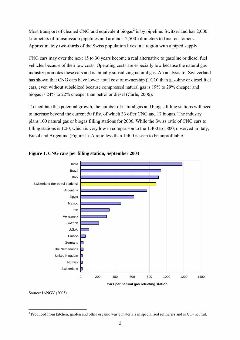
To facilitate this potential growth, the number of natural gas and biogas filling stations will need to increase beyond the current 50 fifty, of which 33 offer CNG and 17 biogas. The industry plans 100 natural gas or biogas filling stations for 2006. While the Swiss ratio of CNG cars to filling stations is 1:20, which is very low in comparison to the 1:400 to1:800, observed in Italy, Brazil and Argentina (Figure 1). A ratio less than 1:400 is seen to be unprofitable.

Figure 1. CNG cars per filling station, September 2003

0 200 400 600 800 1000 1200 1400

India

Brazil

Italy

Switzerland (for petrol stations)

Argentina

Egypt

Mexico

Iran

Venezuela

Sweden

U.S.A.

France

Germany

The Netherlands

United Kingdom

Norway

Switzerland

Cars per natural gas refueling station

Source: IANGV (2005)

2 Produced from kitchen, garden and other organic waste materials in specialised refineries and is CO2 neutral.

3

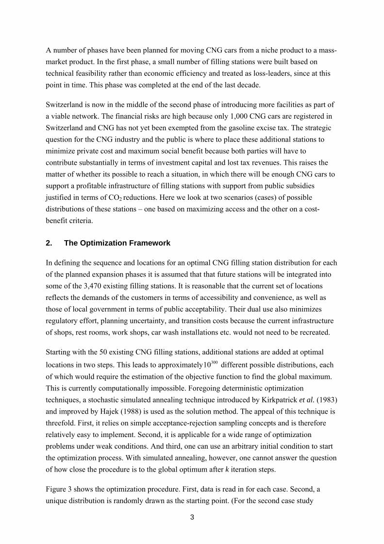
A number of phases have been planned for moving CNG cars from a niche product to a mass-market product. In the first phase, a small number of filling stations were built based on technical feasibility rather than economic efficiency and treated as loss-leaders, since at this point in time. This phase was completed at the end of the last decade.

Switzerland is now in the middle of the second phase of introducing more facilities as part of a viable network. The financial risks are high because only 1,000 CNG cars are registered in Switzerland and CNG has not yet been exempted from the gasoline excise tax. The strategic question for the CNG industry and the public is where to place these additional stations to minimize private cost and maximum social benefit because both parties will have to contribute substantially in terms of investment capital and lost tax revenues. This raises the matter of whether its possible to reach a situation, in which there will be enough CNG cars to support a profitable infrastructure of filling stations with support from public subsidies justified in terms of CO2

reductions. Here we look at two scenarios (cases) of possible distributions of these stations – one based on maximizing access and the other on a cost-benefit criteria.

2. The Optimization Framework

In defining the sequence and locations for an optimal CNG filling station distribution for each of the planned expansion phases it is assumed that that future stations will be integrated into some of the 3,470 existing filling stations. It is reasonable that the current set of locations reflects the demands of the customers in terms of accessibility and convenience, as well as those of local government in terms of public acceptability. Their dual use also minimizes regulatory effort, planning uncertainty, and transition costs because the current infrastructure of shops, rest rooms, work shops, car wash installations etc. would not need to be recreated.

Starting with the 50 existing CNG filling stations, additional stations are added at optimal

locations in two steps. This leads to approximately 30010 different possible distributions, each of which would require the estimation of the objective function to find the global maximum. This is currently computationally impossible. Foregoing deterministic optimization techniques, a stochastic simulated annealing technique introduced by Kirkpatrick et al. (1983) and improved by Hajek (1988) is used as the solution method. The appeal of this technique is threefold. First, it relies on simple acceptance-rejection sampling concepts and is therefore relatively easy to implement. Second, it is applicable for a wide range of optimization problems under weak conditions. And third, one can use an arbitrary initial condition to start the optimization process. With simulated annealing, however, one cannot answer the question of how close the procedure is to the global optimum after k iteration steps.

Figure 3 shows the optimization procedure. First, data is read in for each case. Second, a unique distribution is randomly drawn as the starting point. (For the second case study

4

examined, the number of CNG cars per municipality is calculated using a car ownership multinomial logit model – MNL.) This is followed by the calculation of the initial score of the

objective function{ }( ), nU x x∈ℜ⊆v v ¡ that does not necessarily have a unique maximum.

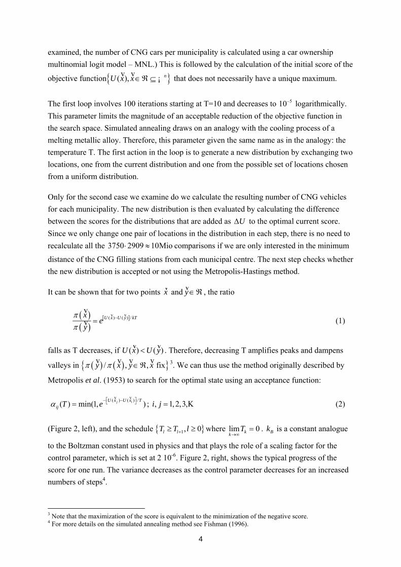
The first loop involves 100 iterations starting at T=10 and decreases to 510− logarithmically. This parameter limits the magnitude of an acceptable reduction of the objective function in the search space. Simulated annealing draws on an analogy with the cooling process of a melting metallic alloy. Therefore, this parameter given the same name as in the analogy: the temperature T. The first action in the loop is to generate a new distribution by exchanging two locations, one from the current distribution and one from the possible set of locations chosen from a uniform distribution.

Only for the second case we examine do we calculate the resulting number of CNG vehicles for each municipality. The new distribution is then evaluated by calculating the difference between the scores for the distributions that are added as UΔ to the optimal current score. Since we only change one pair of locations in the distribution in each step, there is no need to recalculate all the 3750 2909 10Mio⋅ ≈ comparisons if we are only interested in the minimum

distance of the CNG filling stations from each municipal centre. The next step checks whether the new distribution is accepted or not using the Metropolis-Hastings method.

It can be shown that for two points xv and y∈ℜv , the ratio

( )( )

[ ]( ) ( ) /U x U y kTxe

yππ

−=v v

vv (1)

falls as T decreases, if ( ) ( )U x U y<v v . Therefore, decreasing T amplifies peaks and dampens

valleys in ( ) ( ){ }/ , , fixy x y xπ π ∈ℜv v v v 3. We can thus use the method originally described by

Metropolis et al. (1953) to search for the optimal state using an acceptance function:

( ) ( ) /( ) min(1, )j iU x U x Tij T eα ⎡ ⎤− −⎣ ⎦=

v v; , 1, 2,3,i j = K (2)

(Figure 2, left), and the schedule { }1, 0l lT T l+≥ ≥ where lim 0kkT

→∞= . Bk is a constant analogue

to the Boltzman constant used in physics and that plays the role of a scaling factor for the control parameter, which is set at 2 10-6. Figure 2, right, shows the typical progress of the score for one run. The variance decreases as the control parameter decreases for an increased numbers of steps4.

3 Note that the maximization of the score is equivalent to the minimization of the negative score. 4 For more details on the simulated annealing method see Fishman (1996).

5

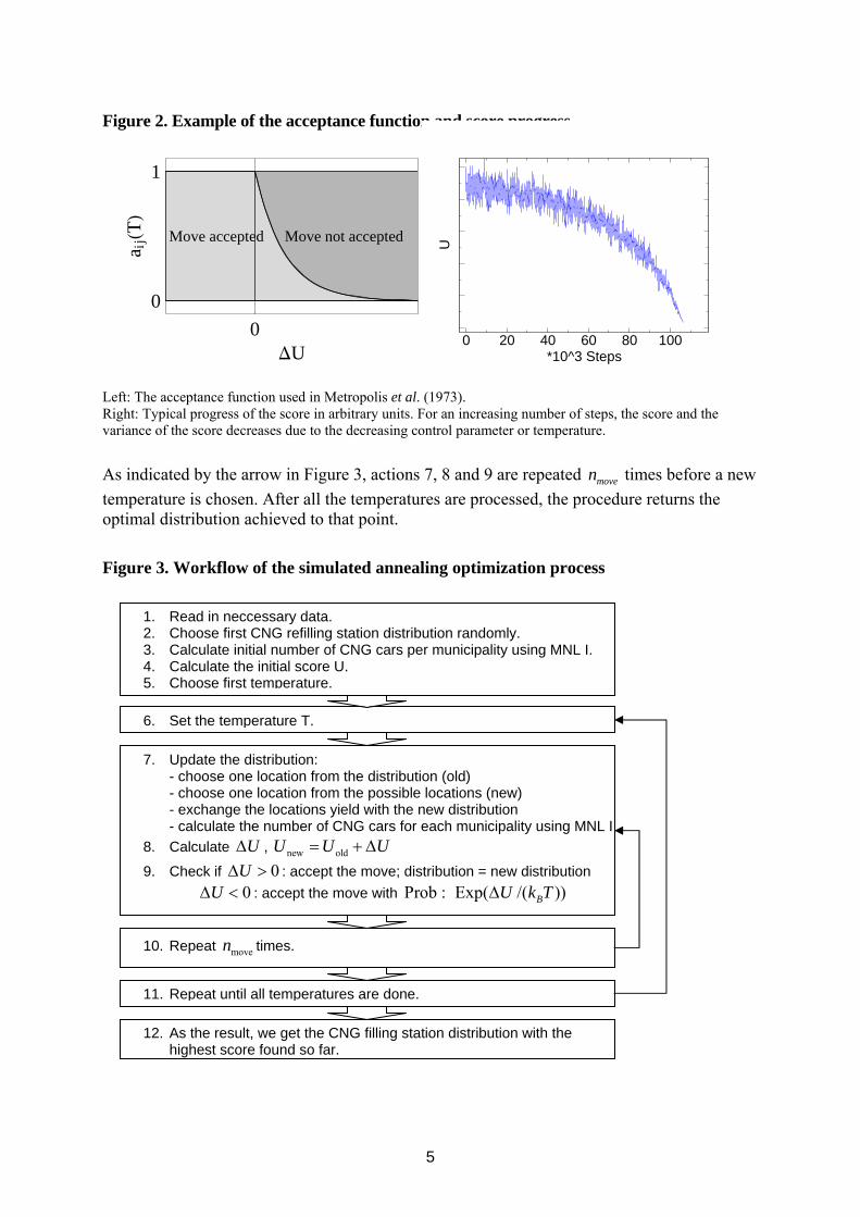
Figure 2. Example of the acceptance function and score progress

0�U

0

1

a ij�T�

Move accepted Move not accepted

0 20 40 60 80 100*10^3 Steps

U

Left: The acceptance function used in Metropolis et al. (1973). Right: Typical progress of the score in arbitrary units. For an increasing number of steps, the score and the variance of the score decreases due to the decreasing control parameter or temperature. As indicated by the arrow in Figure 3, actions 7, 8 and 9 are repeated moven times before a new temperature is chosen. After all the temperatures are processed, the procedure returns the optimal distribution achieved to that point.

Figure 3. Workflow of the simulated annealing optimization process

6. Set the temperature T.

1. Read in neccessary data. 2. Choose first CNG refilling station distribution randomly. 3. Calculate initial number of CNG cars per municipality using MNL I. 4. Calculate the initial score U. 5. Choose first temperature.

7. Update the distribution: - choose one location from the distribution (old) - choose one location from the possible locations (new) - exchange the locations yield with the new distribution - calculate the number of CNG cars for each municipality using MNL I

8. Calculate UΔ , new oldU U U= + Δ

9. Check if 0UΔ > : accept the move; distribution = new distribution 0UΔ < : accept the move with Prob Exp( /( ))BU k TΔ:

11. Repeat until all temperatures are done.

12. As the result, we get the CNG filling station distribution with the highest score found so far.

10. Repeat moven times.

6

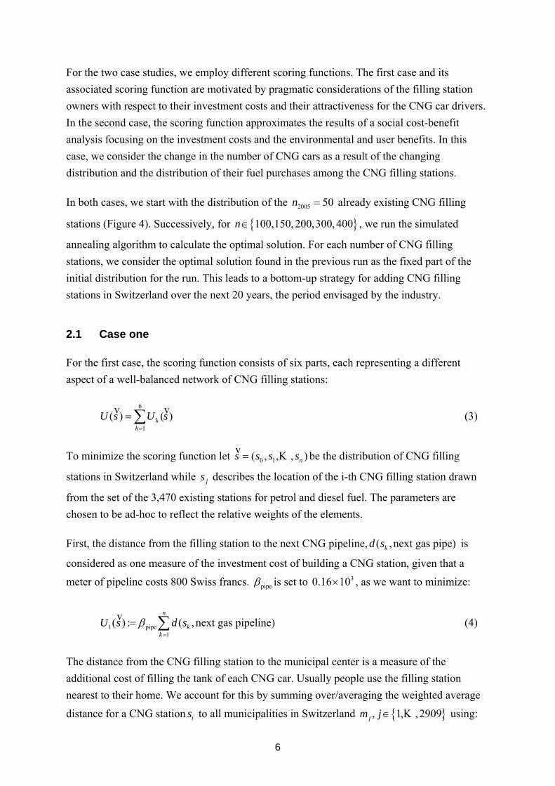
For the two case studies, we employ different scoring functions. The first case and its associated scoring function are motivated by pragmatic considerations of the filling station owners with respect to their investment costs and their attractiveness for the CNG car drivers. In the second case, the scoring function approximates the results of a social cost-benefit analysis focusing on the investment costs and the environmental and user benefits. In this case, we consider the change in the number of CNG cars as a result of the changing distribution and the distribution of their fuel purchases among the CNG filling stations.

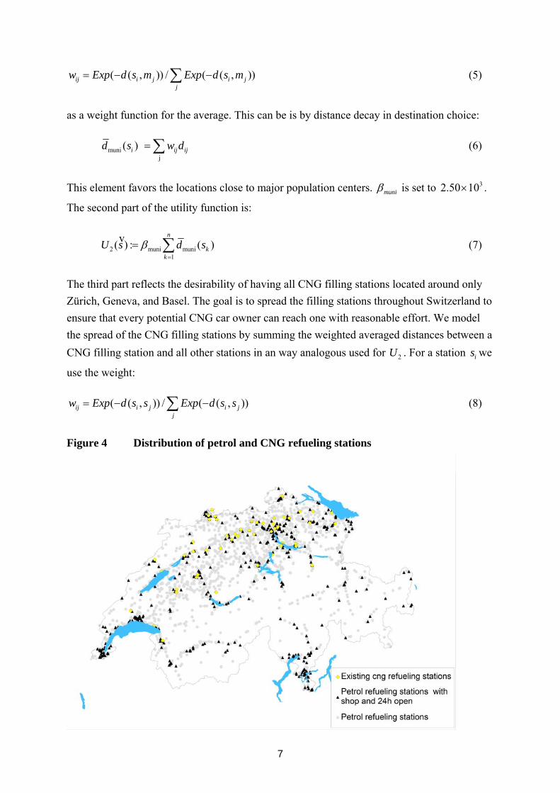
In both cases, we start with the distribution of the 2005 50n = already existing CNG filling

stations (Figure 4). Successively, for { }100,150, 200,300, 400n∈ , we run the simulated

annealing algorithm to calculate the optimal solution. For each number of CNG filling stations, we consider the optimal solution found in the previous run as the fixed part of the initial distribution for the run. This leads to a bottom-up strategy for adding CNG filling stations in Switzerland over the next 20 years, the period envisaged by the industry.

2.1 Case one

For the first case, the scoring function consists of six parts, each representing a different aspect of a well-balanced network of CNG filling stations:

6

1( ) ( )k

kU s U s

=

= ∑v v (3)

To minimize the scoring function let 0 1( , , , )ns s s s=v K be the distribution of CNG filling

stations in Switzerland while js describes the location of the i-th CNG filling station drawn

from the set of the 3,470 existing stations for petrol and diesel fuel. The parameters are chosen to be ad-hoc to reflect the relative weights of the elements.

First, the distance from the filling station to the next CNG pipeline, ( , next gas pipe)kd s is

considered as one measure of the investment cost of building a CNG station, given that a

meter of pipeline costs 800 Swiss francs. pipeβ is set to 30.16 10× , as we want to minimize:

1 pipe1

( ) : ( , next gas pipeline)n

kk

U s d sβ=

= ∑v (4)

The distance from the CNG filling station to the municipal center is a measure of the additional cost of filling the tank of each CNG car. Usually people use the filling station nearest to their home. We account for this by summing over/averaging the weighted average

distance for a CNG station is to all municipalities in Switzerland { }, 1, , 2909jm j∈ K using:

7

( ( , )) / ( ( , ))ij i j i jj

w Exp d s m Exp d s m= − −∑ (5)

as a weight function for the average. This can be is by distance decay in destination choice:

munij

( ) i ij ijd s w d=∑ (6)

This element favors the locations close to major population centers. muniβ is set to 32.50 10× .

The second part of the utility function is:

2 muni muni1

( ) : ( )n

kk

U s d sβ=

= ∑v (7)

The third part reflects the desirability of having all CNG filling stations located around only Zürich, Geneva, and Basel. The goal is to spread the filling stations throughout Switzerland to ensure that every potential CNG car owner can reach one with reasonable effort. We model the spread of the CNG filling stations by summing the weighted averaged distances between a CNG filling station and all other stations in an way analogous used for 2U . For a station is we

use the weight:

( ( , )) / ( ( , ))ij i j i jj

w Exp d s s Exp d s s= − −∑ (8)

Figure 4 Distribution of petrol and CNG refueling stations

8

and for the weighted average distance to all other CNG filling stations we use:

gasj

( ) i ij ijd s w d=∑ (9)

For the third part of the scoring function we get:

3 gas gas1

( ) : ( )n

kk

U s d sβ=

= ∑v (10)

gasβ is set to 31.33 10× , as we want to spread out the stations out.

If we assume that today’s car drivers will change to CNG cars, then it is desirable to build CNG stations close to regions with high car density. To capture this, we car5km ( )jn s is

calculated as the number of cars within 5 km of a possible station location js . A higher

car5km ( )jn s should reduce the score, so the car5kmβ is set to 32.86 10− × leading to:

4 car5km car5km1

( ) : ( )n

kk

U s n sβ=

= ∑v (11)

In addition, for the profitability of a station in selling CNG, it is also important whether it has a shop and its opening hours. To model this, two Boolean terms are used: one for the shop,

shop ( )jb s and one for opening hours 24h ( )jb s . If js has a shop, then shop ( ) 1jb s = , otherwise 0 is

used. Analogously, 24h ( ) 1jb s = if js is open 24 hours a day and 0 otherwise. shopβ and 24hβ are

set to 31.00 10− × and 30.67 10− × , because the presence of the attribute is deemed preferable giving:

5 shop shop1

( ) : ( )n

kk

U s b sβ=

= ∑v (12)

and

6 24h 24h1

( ) : ( )n

kk

U s b sβ=

= ∑v (13)

2.2 Case two

The aim of the second objective function is to balance the social costs and benefits of an investment in CNG filling stations and the vehicles dependent on them. This cost – benefit

9

calculation cannot be completed curently, but it covers the central elements employing the best available estimates for unit costs and benefits. The first term describes the benefits gained from a reduction of CO2 emissions:

2

veh1 CO j

j

U Nα= ∑ (14)

where vehjN is the number of CNG vehicles in each municipality and

2CO 6.61SFR/(year cngvehicle)α = due to the annual CO2 reduction per CNG car. Carle (2006)

calculates that an average compressed natural gas car emits 47.91 grams less CO2 per km. This leads to an annual CO2 savings valued at 6.61 Swiss francs assuming that an average Swiss car travels 12,847 km (Bundesamt für Raumentwicklung, 2001) and that a ton of CO2 costs 9.13 euro (European Energy Exchange AG, 2005).

Second, we consider the benefits from the lower total cost of owning CNG as compared to conventional cars. According to Carle (2004), the cost of ownership of a petrol car in 2004 was 0.86 Swiss francs per km.. For a CNG car, the cost of ownership was at 0.84 Swiss francs.

Taking TCO jΔ as the amount of Swiss francs saved by using a CNG car for each

municipality, for the 2,909 municipalities, we have an average TCO 425.1 119.1Δ = ± Swiss francs with a range of 276.3 to 884.0 francs. The score is:

veh2 TCO j j

j

U N= Δ∑ (15)

We also, however, have to take the costs arising from building the infrastructure into account. These consist of the fixed costs for each additional CNG filling station and the cost for connecting each station to the next CNG pipeline. In addition, we assume that the operation of a CNG filling station is cost effective only when a certain number of CNG car drivers use it. Hence, we have the costs 3U

3 build cnggs pl pl ( )i

U N d iα α= + ∑ (16)

The cost for building one CNG filling station is fix 40000 SFR/(year refilling station)α = −

(Industrielle Werke Basel, 2003). This covers the tank, pressure pumps, its underground burial, and the installation of the pumps. There are no additional costs because we only consider installation at existing stations. Given the small number of stations, we do not expect major cost reductions for this hardware element.

10

Full investment costs are included as the equipment no residual value if a station is closed.

cnggsN is the total number of CNG filling stations considered, pl 20000 SFR/(km year)α = − is

the annual cost of the pipeline per unit length assuming a depreciation period of 40 years, and

pl ( )d i is the distance from the filling station to the next pipeline in kilometers. The

profitability term for CNG filling stations is thus:

4 gsto gsvc gsfc cnggsi ii i

U N N Nα α α= + +∑ ∑% % (17)

The first summation is the turnover, the second is the variable costs of the CNG filling stations and the third is the fixed costs. The turnover coefficient is gsto 1172 SFR/yearα = ,

which is the amount of CNG times the average price for CNG in 2004 based on trading rates. We have gsvc 970 SFR/yearα = − for each CNG car, reflecting the loss of fuel turnover. The

fixed cost for each gas station is gsfc 88536 SFR/yearα = − . iN% is the annual number of CNG

cars using this filling station and is calculated from a multi-nomial logit model that distributes the CNG cars in each municipality to the available filling stations. It is assumed that initially staff is shared with the other facilities at the location (e.g., shop and gasoline pumps).

3. Data

The first case is based on the existing 3,470 petrol and diesel filling stations, of which 1,142 have a shop and, to the best of our knowledge, 875 are open 24 hours a day. The data was collected from a survey of major chains in spring 2004. It was cross-checked against the entries for filling stations in the electronic phone book (Swisscom Directories, 2003) that was also used to identify the non-chain affiliated filling stations. The stations with shop and all-day opening hours are concentrated in cities and larger towns.

The distances between filling stations and to all 2,909 municipalities were calculated using MapInfo 7.5 on the basis of the Microdrive Network (MicroGIS, 2003) – Table 1. The same network was use to calculate the number of cars within 5 km distance of each station. The distribution of cars was obtained from the Swiss Federal Roads Authority (ASTRA, 2004).

There is no public information on the locations of low-pressure CNG pipelines for Switzerland, but the locations of houses with CNG heating and cooking are available from the Swiss Federal Office of Statistics (Bundesamt für Statistik, 2000). Assuming that the pipelines are located in the right-of-way of the streets in front of such houses, a virtual low-pressure pipeline network was constructed. The shortest distance from a filling station location to the nearest street with a filling pipeline was calculated using the road network.

11

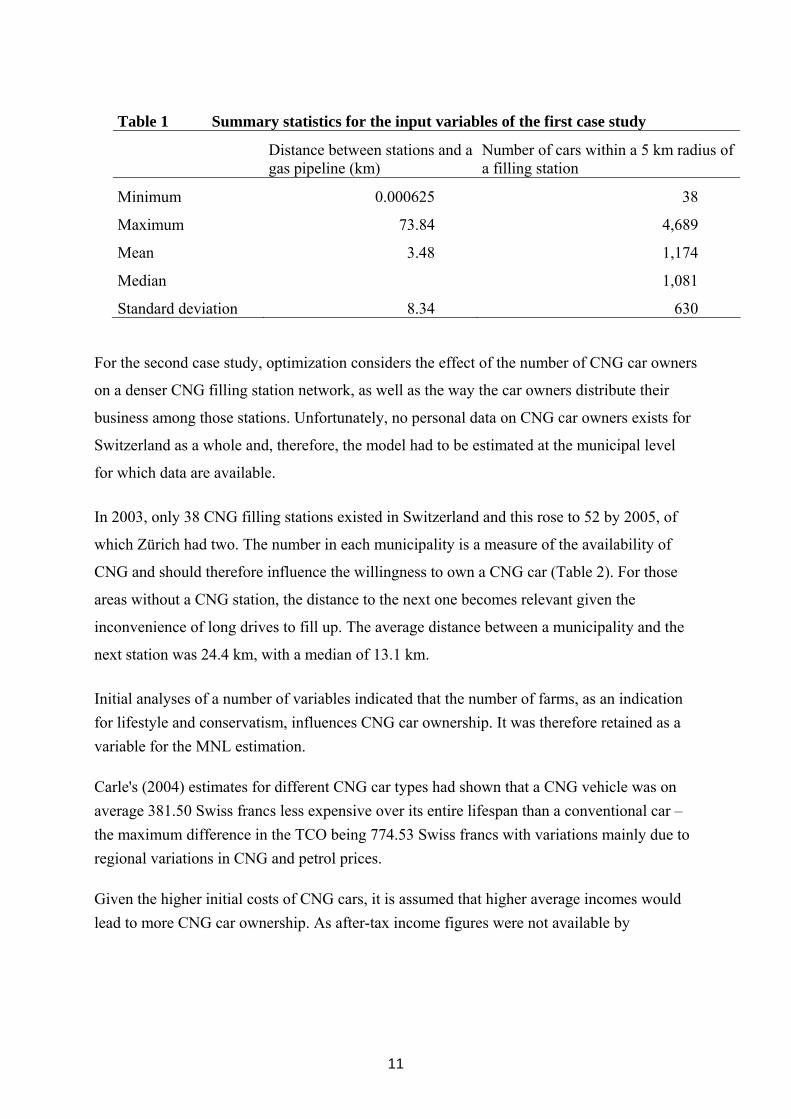
Table 1 Summary statistics for the input variables of the first case study

Distance between stations and a gas pipeline (km)

Number of cars within a 5 km radius of a filling station

Minimum 0.000625 38

Maximum 73.84 4,689

Mean 3.48 1,174

Median 1,081

Standard deviation 8.34 630

For the second case study, optimization considers the effect of the number of CNG car owners

on a denser CNG filling station network, as well as the way the car owners distribute their

business among those stations. Unfortunately, no personal data on CNG car owners exists for

Switzerland as a whole and, therefore, the model had to be estimated at the municipal level

for which data are available.

In 2003, only 38 CNG filling stations existed in Switzerland and this rose to 52 by 2005, of

which Zürich had two. The number in each municipality is a measure of the availability of

CNG and should therefore influence the willingness to own a CNG car (Table 2). For those

areas without a CNG station, the distance to the next one becomes relevant given the

inconvenience of long drives to fill up. The average distance between a municipality and the

next station was 24.4 km, with a median of 13.1 km.

Initial analyses of a number of variables indicated that the number of farms, as an indication for lifestyle and conservatism, influences CNG car ownership. It was therefore retained as a variable for the MNL estimation.

Carle's (2004) estimates for different CNG car types had shown that a CNG vehicle was on average 381.50 Swiss francs less expensive over its entire lifespan than a conventional car – the maximum difference in the TCO being 774.53 Swiss francs with variations mainly due to regional variations in CNG and petrol prices.

Given the higher initial costs of CNG cars, it is assumed that higher average incomes would lead to more CNG car ownership. As after-tax income figures were not available by

12

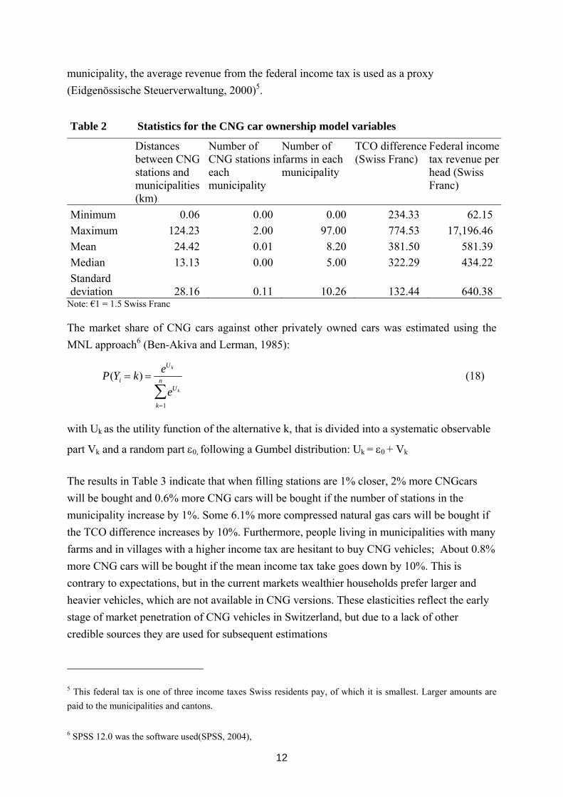
municipality, the average revenue from the federal income tax is used as a proxy (Eidgenössische Steuerverwaltung, 2000)5.

Table 2 Statistics for the CNG car ownership model variables

Distances between CNG stations and municipalities (km)

Number of CNG stations ineach municipality

Number of farms in each municipality

TCO difference (Swiss Franc)

Federal income tax revenue per head (Swiss Franc)

Minimum 0.06 0.00 0.00 234.33 62.15 Maximum 124.23 2.00 97.00 774.53 17,196.46 Mean 24.42 0.01 8.20 381.50 581.39 Median 13.13 0.00 5.00 322.29 434.22 Standard deviation 28.16 0.11 10.26 132.44 640.38

Note: €1 = 1.5 Swiss Franc

The market share of CNG cars against other privately owned cars was estimated using the MNL approach6 (Ben-Akiva and Lerman, 1985):

P(Yi = k) = eUk

eUk

k=1

n

∑ (18)

with Uk as the utility function of the alternative k, that is divided into a systematic observable

part Vk and a random part ε0, following a Gumbel distribution: Uk = ε0 + Vk

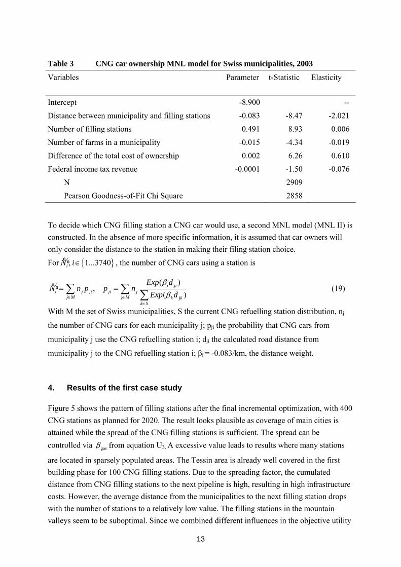
The results in Table 3 indicate that when filling stations are 1% closer, 2% more CNGcars will be bought and 0.6% more CNG cars will be bought if the number of stations in the municipality increase by 1%. Some 6.1% more compressed natural gas cars will be bought if the TCO difference increases by 10%. Furthermore, people living in municipalities with many farms and in villages with a higher income tax are hesitant to buy CNG vehicles; About 0.8% more CNG cars will be bought if the mean income tax take goes down by 10%. This is contrary to expectations, but in the current markets wealthier households prefer larger and heavier vehicles, which are not available in CNG versions. These elasticities reflect the early stage of market penetration of CNG vehicles in Switzerland, but due to a lack of other credible sources they are used for subsequent estimations

5 This federal tax is one of three income taxes Swiss residents pay, of which it is smallest. Larger amounts are paid to the municipalities and cantons.

6 SPSS 12.0 was the software used(SPSS, 2004),

13

Table 3 CNG car ownership MNL model for Swiss municipalities, 2003

Variables Parameter t-Statistic Elasticity

Intercept -8.900 --

Distance between municipality and filling stations -0.083 -8.47 -2.021

Number of filling stations 0.491 8.93 0.006

Number of farms in a municipality -0.015 -4.34 -0.019

Difference of the total cost of ownership 0.002 6.26 0.610

Federal income tax revenue -0.0001 -1.50 -0.076

N 2909

Pearson Goodness-of-Fit Chi Square 2858

To decide which CNG filling station a CNG car would use, a second MNL model (MNL II) is constructed. In the absence of more specific information, it is assumed that car owners will only consider the distance to the station in making their filing station choice.

For { }, 1...3740iN i∈% , the number of CNG cars using a station is

( ),

( )i ji

i j ji ji jj M j M k jk

k S

Exp dN n p p n

Exp dββ∈ ∈

∈

= =∑ ∑ ∑% (19)

With M the set of Swiss municipalities, S the current CNG refuelling station distribution, nj

the number of CNG cars for each municipality j; pji the probability that CNG cars from

municipality j use the CNG refuelling station i; dji the calculated road distance from

municipality j to the CNG refuelling station i; βi = -0.083/km, the distance weight.

4. Results of the first case study

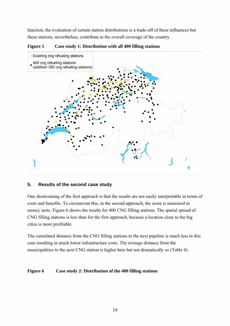
Figure 5 shows the pattern of filling stations after the final incremental optimization, with 400 CNG stations as planned for 2020. The result looks plausible as coverage of main cities is attained while the spread of the CNG filling stations is sufficient. The spread can be controlled via gasβ from equation U3. A excessive value leads to results where many stations

are located in sparsely populated areas. The Tessin area is already well covered in the first building phase for 100 CNG filling stations. Due to the spreading factor, the cumulated distance from CNG filling stations to the next pipeline is high, resulting in high infrastructure costs. However, the average distance from the municipalities to the next filling station drops with the number of stations to a relatively low value. The filling stations in the mountain valleys seem to be suboptimal. Since we combined different influences in the objective utility

14

function, the evaluation of certain station distributions is a trade-off of these influences but these stations, nevertheless, contribute to the overall coverage of the country.

Figure 5 Case study 1: Distribution with all 400 filling stations

5. Results of the second case study

One shortcoming of the first approach is that the results are not easily interpretable in terms of costs and benefits. To circumvent this, in the second approach, the score is measured in money units. Figure 6 shows the results for 400 CNG filling stations. The spatial spread of CNG filling stations is less than for the first approach, because a location close to the big cities is more profitable.

The cumulated distance from the CNG filling stations to the next pipeline is much less in this case resulting in much lower infrastructure costs. The average distance from the municipalities to the next CNG station is higher here but not dramatically so (Table 4).

Figure 6 Case study 2: Distribution of the 400 filling stations

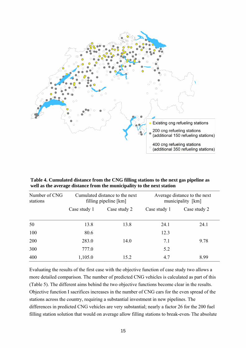
15

Table 4. Cumulated distance from the CNG filling stations to the next gas pipeline as well as the average distance from the municipality to the next station

Number of CNG stations

Cumulated distance to the next filling pipeline [km]

Average distance to the next municipality [km]

Case study 1

Case study 2

Case study 1

Case study 2

50 13.8 13.8 24.1 24.1

100 80.6 12.3

200 283.0 14.0 7.1 9.78

300 777.0 5.2

400 1,105.0 15.2 4.7 8.99

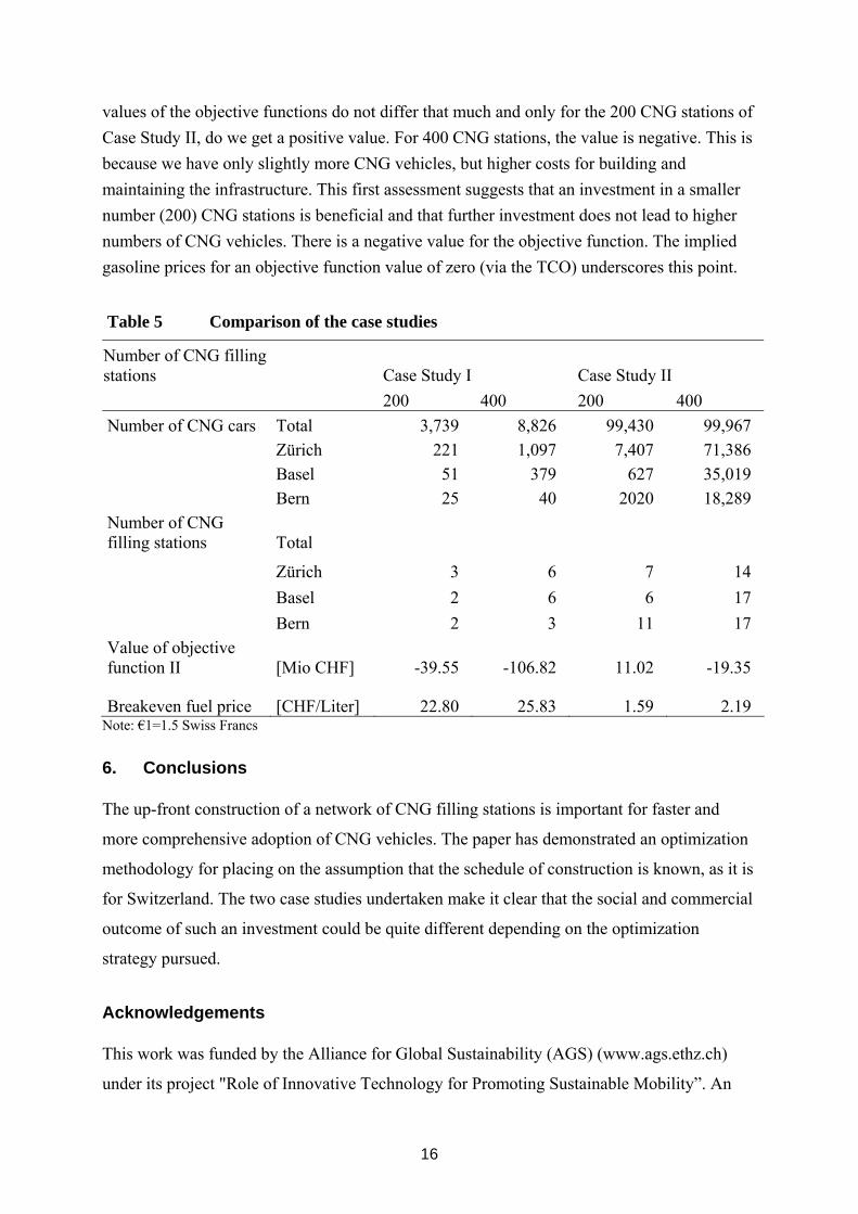
Evaluating the results of the first case with the objective function of case study two allows a more detailed comparison. The number of predicted CNG vehicles is calculated as part of this (Table 5). The different aims behind the two objective functions become clear in the results. Objective function I sacrifices increases in the number of CNG cars for the even spread of the stations across the country, requiring a substantial investment in new pipelines. The differences in predicted CNG vehicles are very substantial; nearly a factor 26 for the 200 fuel filling station solution that would on average allow filling stations to break-even. The absolute

16

values of the objective functions do not differ that much and only for the 200 CNG stations of Case Study II, do we get a positive value. For 400 CNG stations, the value is negative. This is because we have only slightly more CNG vehicles, but higher costs for building and maintaining the infrastructure. This first assessment suggests that an investment in a smaller number (200) CNG stations is beneficial and that further investment does not lead to higher numbers of CNG vehicles. There is a negative value for the objective function. The implied gasoline prices for an objective function value of zero (via the TCO) underscores this point.

Table 5 Comparison of the case studies

Number of CNG filling stations Case Study I Case Study II 200 400 200 400 Number of CNG cars Total 3,739 8,826 99,430 99,967 Zürich 221 1,097 7,407 71,386 Basel 51 379 627 35,019 Bern 25 40 2020 18,289 Number of CNG filling stations Total

Zürich 3 6 7 14 Basel 2 6 6 17 Bern 2 3 11 17 Value of objective function II [Mio CHF] -39.55 -106.82 11.02 -19.35

Breakeven fuel price [CHF/Liter] 22.80 25.83 1.59 2.19 Note: €1=1.5 Swiss Francs

6. Conclusions

The up-front construction of a network of CNG filling stations is important for faster and

more comprehensive adoption of CNG vehicles. The paper has demonstrated an optimization

methodology for placing on the assumption that the schedule of construction is known, as it is

for Switzerland. The two case studies undertaken make it clear that the social and commercial

outcome of such an investment could be quite different depending on the optimization

strategy pursued.

Acknowledgements

This work was funded by the Alliance for Global Sustainability (AGS) (www.ags.ethz.ch)

under its project "Role of Innovative Technology for Promoting Sustainable Mobility”. An

17

earlier version of the paper was presented at the Annual Meeting of the Transportation

Research Board.

References

ASTRA (2004) Bestand an Personenwagen nach verschiedenen Treibstoffarten, ASTRA, Bern.

Bundesamt für Raumentwicklung (BFS) (2001) Mobilität in der Schweiz, Ergebnisse des Mikrozensus 2000 zum Verkehrsverhalten, Bundesamt für Raumentwicklung, Bundesamt für Statistik, Bern und Neuenburg.

Bundesamt für Statistik (2000) Eidgenössisches Gebäude- und Wohnungsregister, Merkmalskatalog - Version 2.3 of 19. Oktober 2000, Bundesamt für Statistik, Neuenburg.

Carle, G. (2004) Erdgasfahrzeuge im Wettbewerb, Arbeitsbericht Verkehrs- und Raumplanung, 269, IVT, ETH Zürich, Zürich.

Carle, G. (2006) Erdgasfahrzeuge und ihr Beitrag zu einer CO2Reduktion im motorisierten Personenverkehr der Schweiz, Dissertation, ETH Zürich, Zürich.

Cleaner Drive (2003) Wie sauber fährt Dein Auto, http://www.cleaner-drive.ch/tools/news.cfm?lang=de, Cleaner Drive, November 2003.

Eidgenössische Steuerverwaltung (2000) Steuerstatistik - Direkte Bundessteuer- Natürliche Personen, , http://www.estv.admin.ch/data/sd/d/index.htm, Eidg. Steuerverwaltung, Bern, 1.12.2004.

European Energy Exchange AG (2005) CO2-Index, http://www.eex.de/co2_index/carbonindex.xls, European Energy Exchange AG, 12.4.2005.

Fishman, G.S. (1996) Monte Carlo Concepts, Algorithms, and Applications, Springer Verlag, New York.

Hajek, B. (1988) Cooling schedules for optimal annealing, Mathematics of OR, 13 311–329. Hastings, W. K. (1970) Monte Carlo sampling methods using Markov chains and their

applications, Biometrika, 57 , 92-109. IANGV, 2004, Latest International NGV Statistics,

www.iangv.org/jaytech/default.php?PageID§=130, NGV. IANGV (2005) Latest International NGV Statistics,

www.iangv.org/jaytech/default.php?PageID=130 NGV, 25.4.2005. Industrielle Werke Basel (2003) Erdgasbetankungsanlagen im Erdgasversorgungsgebiet der

IWB - Errichtung von Erdgasbetankungsanlagen in den Jahren 2003 und 2004, Industrielle Werke Basel (IWB), Basel.

Kirkpatrick, S., C.D. Gelatt Jr., and M.P. Vecchi (1983) Optimization by simulated annealing, Science, 220 (4598) 671–680.

MapInfo (2003) Mapinfo 7.5, Mapinfo, Troy, New York. Metropolis, N., A.W. Rosenbluth, M.N. Rosenbluth, A.H. Teller, and E. Teller (1953)

Equation state calculations by fast computing machines, Journal of Chemical Physics, 21:1087–1092.

MicroGIS (2003) Technische Daten, MicroGIS, St-Sulpice. SPSS (2004) SPSS Inc., SPSS Inc., Chicago. Swisscom directories (2003) telinfo 11/03, Datas Swisscom Directories AG, Bern.