NASA/TM-1998-112223

Optimization of Supersonic Transport Trajectories

Mark D. Ardema, Robert Windhorst, and James Phillips

March 1998

https://ntrs.nasa.gov/search.jsp?R=19980027605 2018-05-26T04:29:08+00:00Z

The NASA STI Program Office... in Profile

Since its founding, NASA has been dedicated to the

advancement of aeronautics and space science. TheNASA Scientific and Technical Information (STI)

Program Office plays a key part in helping NASA

maintain this important role.

The NASA STI Program Office is operated by

Langley Research Center, the Lead Center forNASA's scientific and technical information. The

NASA STI Program Office provides access to the

NASA STI Database, the largest collection of

aeronautical and space science STI in the world.

The Program Office is also NASA's institutional

mechanism for disseminating the results of its

research and development activities. These results

are published by NASA in the NASA STI Report

Series, which includes the following report types:

TECHNICAL PUBLICATION. Reports of

completed research or a major significant phase

of research that present the results of NASA

programs and include extensive data or theoreti-

cal analysis. Includes compilations of significantscientific and technical data and information

deemed to be of continuing reference value.

NASA's counterpart of peer-reviewed formal

professional papers but has less stringent

limitations on manuscript length and extent

of graphic presentations.

TECHNICAL MEMORANDUM. Scientific and

technical findings that are preliminary or of

specialized interest, e.g., quick release reports,working papers, and bibliographies that containminimal annotation. Does not contain extensive

analysis.

• CONTRACTOR REPORT. Scientific and

technical findings by NASA-sponsored

contractors and grantees.

CONFERENCE PUBLICATION. Collected

papers from scientific and technical confer-

ences, symposia, seminars, or other meetings

sponsored or cosponsored by NASA.

SPECIAL PUBLICATION. Scientific, technical,

or historical information from NASA programs,

projects, and missions, often concerned with

subjects having substantial public interest.

TECHNICAL TRANSLATION. English-

language translations of foreign scientific andtechnical material pertinent to NASA's mission.

Specialized services that complement the STI

Program Office's diverse offerings include creatingcustom thesauri, building customized databases,

organizing and publishing research results.., even

providing videos.

For more information about the NASA STI

Program Office, see the following:

• Access the NASA STI Program Home Page at

http ://www.sti.nasa. gov

• E-mail your question via the Internet to

help@sti.nasa.gov

• Fax your question to the NASA Access Help

Desk at (301) 621-0134

• Telephone the NASA Access Help Desk at

(301) 621-0390

Write to:

NASA Access Help DeskNASA Center for AeroSpace Information

800 Elkridge Landing Road

Linthicum Heights, MD 21090-2934

NASA/TMm1998-112223

Optimization of Supersonic Transport Trajectories

Mark D. Ardema and Robert Windhorst

Santa Clara University, Santa Clara, California

James Phillips

Ames Research Center, Moffett Field, California

National Aeronautics and

Space Administration

Ames Research Center

Moffett Field, California 93035-1000

March 1998

NASA Center for AeroSpace Information

800 Elkridge Landing Road

Linthicum Heights, MD 21090-2934

Price Code: A 17

Available from:

National Technical Information Service

5285 Port Royal Road

Springfield, VA 22161Price Code: AI0

CONTENTS

SUMMARY

INTRODUCTION

DYNAMIC MODELING

Equations of Motion .......................................

Transformation to New State Variables .............................

OPTIMAL CONTROL AND SINGULAR PERTURBATIONS

The Maximum Principle .....................................

Approximation Techniques ....................................

Singular Perturbations and Time Scaling ............................

GUIDANCE LAW DEVELOPMENT

Range Dynamics .........................................

Energy Dynamics .........................................

Fast States Dynamics .......................................

NUMERICAL EXAMPLE

CONCLUDING REMARKS

APPENDIX A - NOMENCLATURE

APPENDIX B - NUMERICAL INTEGRATION OF STATE EQUATIONS

Path Following ..........................................

Constant Normal Load Factor (N) Paths ............................

APPENDIX C - NECESSARY CONDITIONS FOR FAST DYNAMICS

REFERENCES

TABLE

FIGURES

1

1

2

2

3

9

9

10

11

15

15

17

19

23

26

27

28

28

29

32

38

41

41

°°,

111

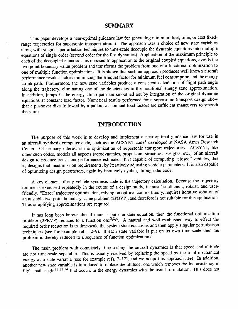
SUMMARY

This paper develops a near-optimal guidance law for generating minimum fuel, time, or cost fixed-

range trajectories for supersonic transport aircraft. The approach uses a choice of new state variables

along with singular perturbation techniques to time-scale decouple the dynamic equations into multiple

equations of single order (second order for the fast dynamics). Application of the maximum principle to

each of the decoupled equations, as opposed to application to the original coupled equations, avoids the

two point boundary value problem and transforms the problem from one of a functional optimization to

one of multiple function optimizations. It is shown that such an approach produces well known aircraft

performance results such as minimizing the Brequet factor for minimum fuel consumption and the energy

climb path. Furthermore, the new state variables produce a consistent calculation of flight path angle

along the trajectory, eliminating one of the deficiencies in the traditional energy state approximation.

In addition, jumps in the energy climb path are smoothed out by integration of the original dynamic

equations at constant load factor. Numerical results performed for a supersonic transport design show

that a pushover dive followed by a pullout at nominal load factors are sufficient maneuvers to smooth

the jump.

INTRODUCTION

The purpose of this work is to develop and implement a near-optimal guidance law for use in

an aircraft synthesis computer code, such as the ACSYNT code 1 developed at NASA Ames Research

Center. Of primary interest is the optimization of supersonic transport trajectories. ACSYNT, like

other such codes, models all aspects (aerodynamics, propulsion, structures, weights, etc.) of an aircraft

design to produce consistent performance estimates. It is capable of computing "closed" vehicles, that

is, designs that meet mission requirements, by iteratively adjusting vehicle parameters. It is also capable

of optimizing design parameters, again by iteratively cycling through the code.

A key element of any vehicle synthesis code is the trajectory calculation. Because the trajectory

routine is exercised repeatedly in the course of a design study, it must be efficient, robust, and user-

friendly. "Exact" trajectory optimization, relying on optimal control theory, requires iterative solution of

an unstable two-point boundary-value problem (2PBVP), and therefore is not suitable for this application.

Thus simplifying approximations are required.

It has long been known that if there is but one state equation, then the functional optimization

problem (2PBVP) reduces to a function one 2'3'4. A natural and well-established way to effect the

required order reduction is to time-scale the system state equations and then apply singular perturbation

techniques (see for example refs. 2-9). If each state variable is put on its own time-scale then the

problem is thereby reduced to a sequence of function optimizations.

The main problem with completely time-scaling the aircraft dynamics is that speed and altitude

are not time-scale separable. This is usually resolved by replacing the speed by the total mechanical

energy as a state variable (see for example refs. 2-12), and we adopt this approach here. In addition,

another new state variable is introduced to replace the altitude, one which removes the inconsistency in

flight path angle 11'13'14 that occurs in the energy dynamics with the usual formulation. This does not

directly impactthe energydynamicssolutionbut increasestheaccuracyof the altitude/flightpathangledynamicssolution.

The energy-stateapproximation(neglectingall dynamicsexceptthe energydynamics)has beenappliedwith successto a wide variety of aircraft, includinghigh performancesupersonicaircraft andlaunchvehicles.It is perhapsbestsuited,however,to transportaircraftbecausethebenignmaneuversofthesevehiclesmaketheassumptionsinvolvedin theenergy-stateapproximation(ESA)lessquestionable.The ESA has been applied most thoroughly to subsonic transport aircraft by Erzberger 15-17. The results

were so satisfactory that the resulting algorithms currently are being used for on-board guidance in

commercial transports.

Applying the ESA to supersonic transports introduces some new features. First, these aircraft have

higher speeds and usually longer ranges than do subsonic aircraft. More importantly, due to the rise in

drag near transonic speeds, they typically have an instantaneous altitude change in their energy-climb

paths. These altitude jumps have been investigated by various means in references 12, 18-22. In this

paper, we use the approach of references 12 and 22 to address this problem.

Finally, some numerical results are presented to demonstrate the utility of the method.

DYNAMIC MODELING

Equations of Motion

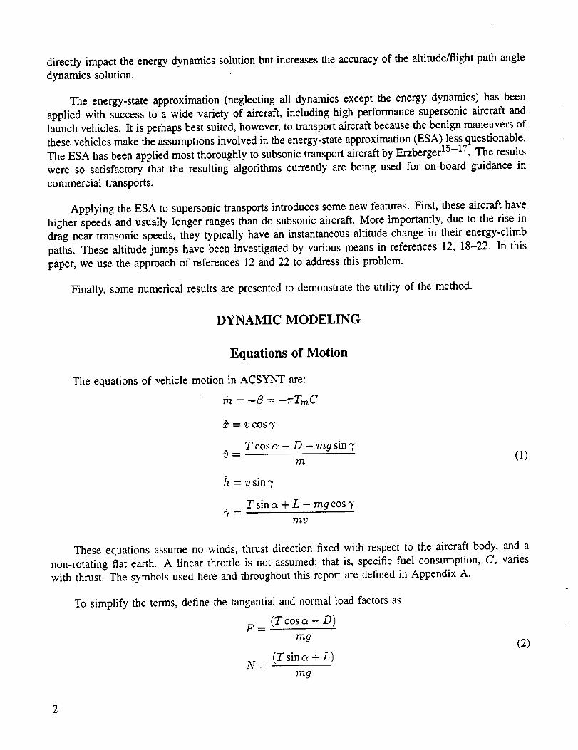
The equations of vehicle motion in ACSYNT are:

= - fl = - Tr C

"- V COS"/

T cos a - D - mg sin 7= (1)

T/2

h = v sin_'

T sin a + L - m9 cos'7

T/g'U

These equations assume no winds, thrust direction fixed with respect to the aircraft body, and a

non-rotating fiat earth. A linear throttle is not assumed; that is, specific fuel consumption, C, varies

with thrust. The symbols used here and throughout this report are defined in Appendix A.

To simplify the terms, define the tangential and normal load factors as

(T cos a - D)F

rag

N= (Tsina+L)rag

(2)

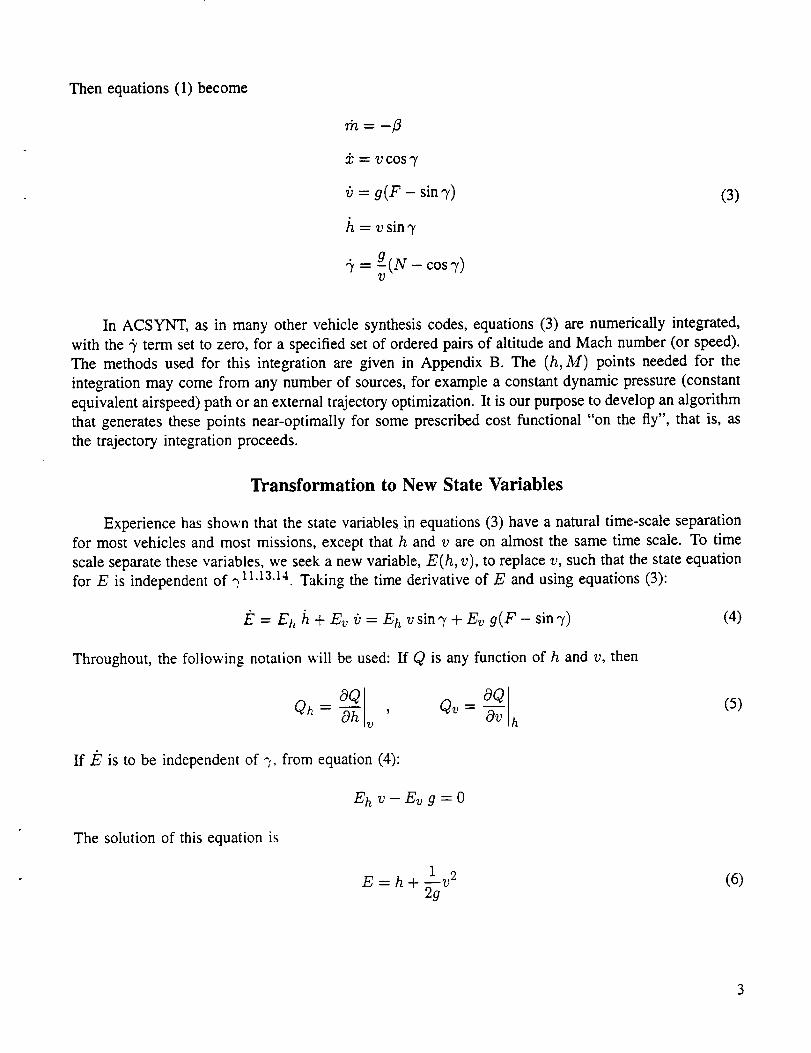
Thenequations(1) become

:/: = v cos"/

i_ = g(F - sinT)

h = vsin7

"_ = g-(N - cos 7)V

(3)

In ACSYNT, as in many other vehicle synthesis codes, equations (3) are numerically integrated,

with the $ term set to zero, for a specified set of ordered pairs of altitude and Mach number (or speed).

The methods used for this integration are given in Appendix B. The (h, M) points needed for the

integration may come from any number of sources, for example a constant dynamic pressure (constant

equivalent airspeed) path or an external trajectory optimization. It is our purpose to develop an algorithm

that generates these points near-optimally for some prescribed cost functional "on the fly", that is, as

the trajectory integration proceeds.

Transformation to New State Variables

Experience has shown that the state variables in equations (3) have a natural time-scale separation

for most vehicles and most missions, except that h and v are on almost the same time scale. To time

scale separate these variables, we seek a new variable, E(h, v), to replace v, such that the state equation

for E is independent of _11.13.14. Taking the time derivative of E and using equations (3):

iF = Eh h + Ev _ = Eh v sin 7 + Ev g(F - sin 7)

Throughout, the following notation will be used: If Q is any function of h and v, then

(4)

OQ hQh=aO , (s)

If/_ is to be independent of ";,, from equation (4):

Eh v-Evg---O

1 2

E=h+_gv

The solution of this equation is

(6)

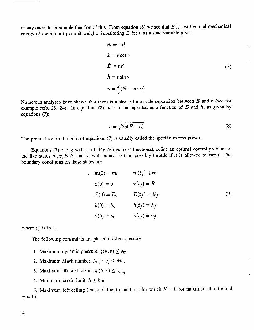
or anyonce-differentiablefunctionof this. Fromequation(6) we seethatE is just the total mechanical

energy of the aircraft per unit weight. Substituting E for v as a state variable gives

rh=-fl

5: = v COS"/

= vF (7)

h = vsin7

,_= g(N - cos7)v

Numerous analyses have shown that there is a strong time-scale separation between E and h (see for

example refs. 23, 24). In equations (8), v is to be regarded as a function of E and h, as given by

equations (7):

v = V/2g(E- h) (8)

boundary conditions on these states are

m(0) = m0

x(o) = o

E(O) = Eo

h(O)= ho

7(0) = "_0

where ty is free.

re(t:) free

z(t:) = R

E(ts)=EI

h(ty)=hy

7(tf) = 7f

The following constraints are placed on the trajectory:

1. Maximum dynamic pressure, q(h, v) < qm

2. Maximum Mach number, M(h, v) < Mm

3. Maximum lift coefficient, CL(h , v) < CLm

4. Minimum terrain limit, h >_ hm

5. Maximum loft ceiling (locus of flight conditions for which F = 0 for maximum throttle and

7=0)

(9)

The product vF in the third of equations (7) is usually called the specific excess power.

Equations (7), along with a suitably defined cost functional, define an optimal control problem in

the five states m, x, E, h, and '7, with control a (and possibly throttle if it is allowed to vary). The

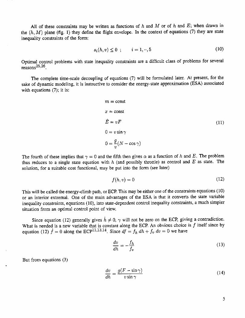
All of theseconstraintsmay bewritten asfunctionsof h and M or of h and E; when drawn in

the (h, M) plane (fig. l) they define the flight envelope. In the context of equations (7) they are state

inequality constraints of the form:

xi(h,v) __ 0 ; i - 1,..,5 (10)

Optimal control problems with state inequality constraints are a difficult class of problems for severalreasons25, 26.

The complete time-scale decoupling of equations (7) will be formulated later. At present, for the

sake of dynamic modeling, it is instructive to consider the energy-state approximation (ESA) associated

with equations (7); it is:

m = const

x = const

.E--vF (11)

0 = v sin3,

0 = g(N - cos- )V

The fourth of these implies that 3' = 0 and the fifth then gives a as a function of h and E. The problem

thus reduces to a single state equation with h (and possibly throttle) as control and E as state. The

solution, for a suitable cost functional, may be put into the form (see later)

f(h,v)--0 (12)

This will be called the energy-climb path, or ECR This may be either one of the constraints equations (10)

or an interior extremal. One of the main advantages of the ESA is that it converts the state variable

inequality constraints, equations (10), into state-dependent control inequality constraints, a much simpler

situation from an optimal control point of view.

Since equation (12) generally gives h ¢ 0, 3' will not be zero on the ECP, giving a contradiction.

What is needed is a new variable that is constant along the ECP. An obvious choice is f itself since by

equation (12) .f = 0 along the ECP n,13,14. Since df = fh dh + fv dv = 0 we have

dv = _fh (13)dh fv

But from equations (3)

dv = g(F - sin_)

dh v sin q'(14)

so that

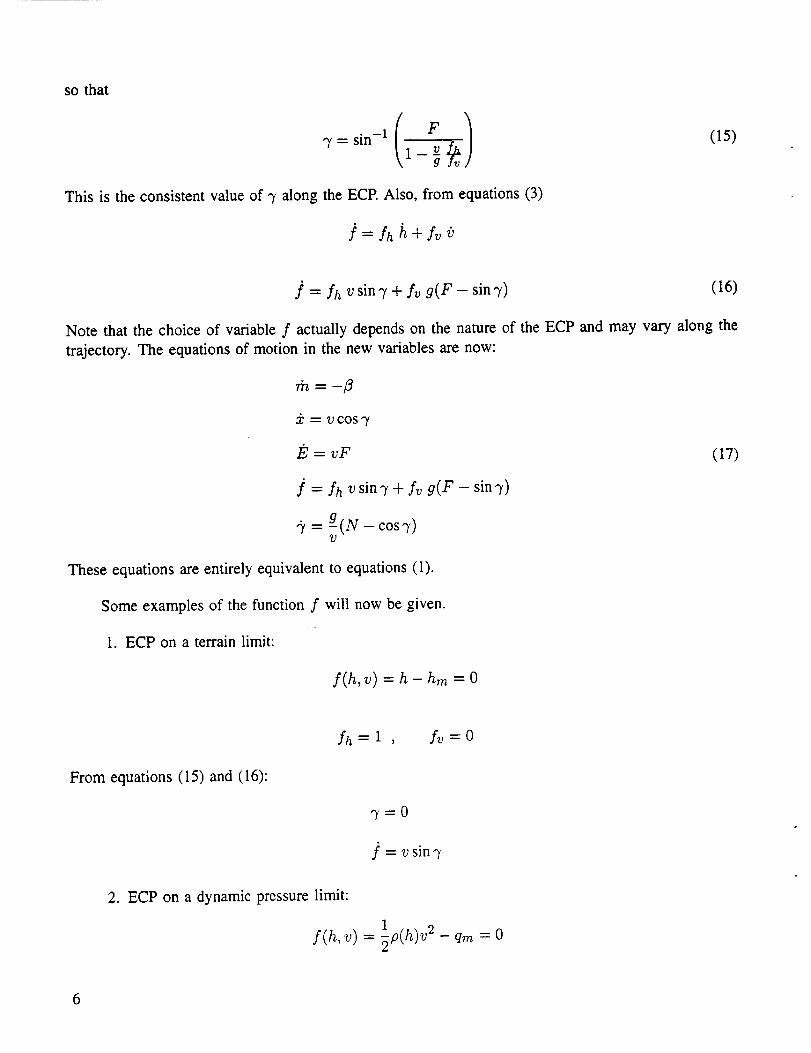
This is the consistentvalueof '7 along the ECR Also, from equations (3)

]=Ah+A

•(15)

] = fh v sin7 + fv 9(F - sinT) (16)

Note that the choice of variable f actually depends on the nature of the ECP and may vary along the

trajectory. The equations of motion in the new variables are now:

m=-_

5: = vcos7

.F, = vF (17)

.f = fh vsin7 + fv g(F - sin7)

= g-(N - cos7)72

These equations are entirely equivalent to equations (1).

Some examples of the function f will now be given.

1. ECP on a terrain limit:

f(h,v)=h-hm=O

From equations (15) and (16):

2. ECP on a dynamic pressure limit:

fh = l , fv = O

f(h,v) -- _p(h)v 2 - qm = 0

6

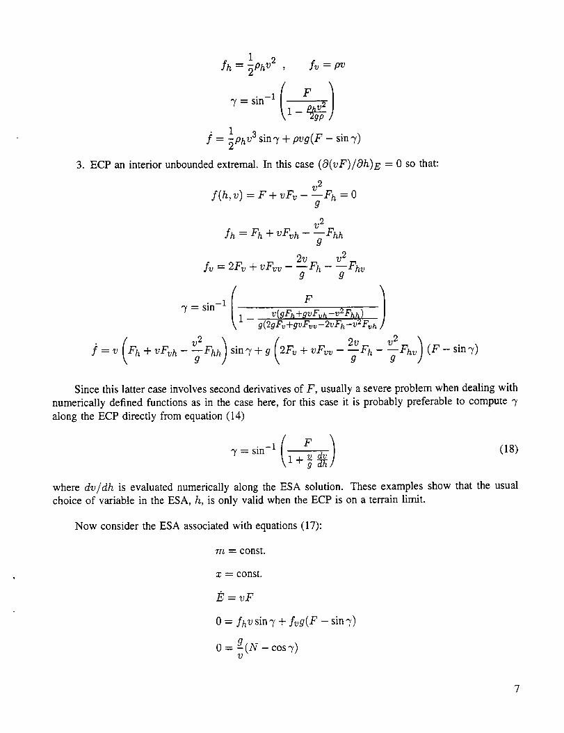
1 2Ih = _phv , f_ = pv

1 3.f' = -_PhV sin-y + pvg(F - sin-),)

3. ECP an interior unbounded extremal. In this case (O(vF)/Oh)E = 0 so that:

v 2f(h,v) = F + vFv- --Fh = O

g

v 2

fh = Fh + v-_h- 7 Fhh2v v 2

fv = 2Fv+ _Fvv- TFh - _Fhv

)1 - v(gFl_WgvFyh-V2Fhh)g(2gFv +gvF,,.-2vFh-v_ Fvh

]=v Fh-t-VFvh-'_-Fhh sin_'+g 2Fv+VFVv-gFh-gFhv (F-sin "y)

Since this latter case involves second derivatives of F, usually a severe problem when dealing with

numerically defined functions as in the case here, for this case it is probably preferable to compute "3,

along the ECP directly from equation (14)

_,=sin_l( F /_) (18)

where dv/dh is evaluated numerically along the ESA solution. These examples show that the usual

choice of variable in the ESA, h, is only valid when the ECP is on a terrain limit.

Now consider the ESA associated with equations (17):

m = const.

x = const.

F_,= vF

0 = fhv sin 7 + fvg(F - sin "f)

0 = g-(N - cos 7)V

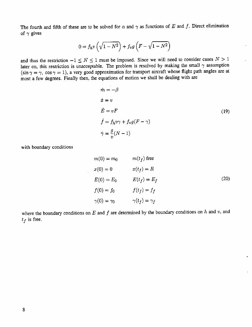
The fourth and fifth of these are to be solved for a and 'T as functions of E and f. Direct elimination

of "7 gives

and thus the restriction -1 < N < 1 must be imposed. Since we will need to consider cases N > 1

later on, this restriction is unacceptable. The problem is resolved by making the small "7 assumption

(sin 7 = "T, cos 3' = 1), a very good approximation for transport aircraft whose flight path angles are at

most a few degrees. Finally then, the equations of motion we shall be dealing with are

with boundary conditions

rh = -_

X"-V

E=vF (19)

] = A_'7+ Ag(F- "7)

g(N- 1)_=v

re(O)= mo re(t:) free

z(O)=O x(ts)=R

E(0) = Eo E(tf)=E f

f(0) =/o f(tf)=f:

"7(0)= "70 "7(t:)= _:

(20)

where the boundary conditions on E and f are determined by the boundary conditions on h and v, and

tf is free.

8

OPTIMAL CONTROL AND SINGULAR PERTURBATIONS

The Maximum Principle

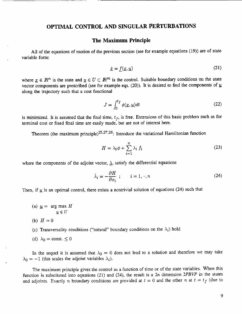
All of the equations of motion of the previous section (see for example equations (19)) are of state

variable form:

z_."= f__(_x,u_) (21)

where _z E ./Rn is the state and u E U c hRm is the control. Suitable boundary conditions on the state

vector components are prescribed (see for example eqs. (20)). It is desired to find the components of u

along the trajectory such that a cost functional

= f0ts ¢(z, u)dtJ (22)

is minimized. It is assumed that the final time, t f, is free. Extensions of this basic problem such as for

terminal cost or fixed final time are easily made, but are not of interest here.

Theorem (the maximum principle)25,2728: Introduce the variational Hamiltonian function

n

H = h0¢ + _ hi fi (23)i=I

where the components of the adjoint vector, _, satisfy the differential equations

),i = OHOxi i = 1,.., n (24)

Then, if _u is an optimal control, there exists a nontrivial solution of equations (24) such that

(a) u= argmaxH

u_EU

(b) H = 0

(c) Transversality conditions ("natural" boundary conditions on the h i) hold

(d) h 0 = const. <_ 0

In the sequel it is assumed that h0 -- 0 does not lead to a solution and therefore we may take

h0 = -1 (this scales the adjoint variables hi).

The maximum principle gives the control as a function of time or of the state variables. When this

function is substituted into equations (21) and (24), the result is a 2n dimension 2PBVP in the states

and adjoints. Exactly n boundary conditions are provided at t = 0 and the other n at t = tf (due to

thetransversalityconditions).Further,theequationsareunstablein the sensethat if they arelinearizedabouta nominal trajectory,one-halfof the systemmatrixeigenvalueswill havepositive real partsandtheothernegative(unlesssomearezero). Although many approaches have been developed to solve this

class of problem, they are all computationally expensive (requiring repetitive solution of the equations),

non-robust (due to the instability), and not user-friendly (requiring extensive input by experts). Thus

they are unsuitable for use in a vehicle synthesis code and approximations must be developed for this

purpose.

Approximation Techniques

Our basic approach is to reduce the complexity of the trajectory optimization problem by seeking

means of reducing the problem to sub-problems of lower order. There are two keys observations in this

regard.

First, suppose there is a state variable, say x j, such that xj does not appear in the system functions

f nor the cost function f0, except for possibly fj, and the final value of xj is unspecified. Then from

equation (24) and the transversality conditions, the differential equation for the corresponding Aj and

its boundary condition are

= ofj , j(t s) = oOxj

The only solution to this linear differential equation for a finite value of Ofj/Oxj is Aj = 0. Thus, from

equation (23), we see that the jth state equation does not influence the optimal control; this equation

has uncoupled from the problem and may be integrated after the optimal control problem has been

solved. This is the reason, for example, that the range equation uncouples from the other equations in

the minimum time-to-climb problem.

Second, suppose that there is only one state equation (z_. is a scalar) and one control variable:

=f(z, u) (25)

with cost functional

tlJ = ¢(x, u)dt

We have then, from equations (23) and (24)

H = -¢ + Af

(26)

0¢ A OfOx Ox

The maximum principle gives, assuming that unbounded optimal control exists,

H = -¢+Af = 0

OH 0¢ Of

Ou - Ou + )_ -_u =O

10

Eliminating ,_ from these two equations gives

=0

This may be thought of as an equation for u as a function of x, i.e., a feedback control law.

Alternatively, a direct approach may be used. Combining equations (25) and (26) gives

J=fotf_dx

(27)

Thus (C/f) is to be minimized with respect to u holding x fixed. Carrying out this minimization for

unbounded control results in exactly equation (27). Actually, a stronger result holds for the single state

case; if u__is a bounded control of several components, then the optimal control is given by 2,3

ar min(;)u__E U x=const

(28)

Singular Perturbations and Time Scaling

We have just seen that if the dynamic system can be approximated by a single state equation, or by

a series of such equations, then the solution may be obtained by elementary means, without solving the

2PBVP. Singular perturbation theory provides a framework for accomplishing this, and indeed many of

the references cited in the Introduction use this approach.

The extensive literature on the application of singular perturbation theory to optimal control prob-

lems in general and flight path optimization in particular will only be reviewed briefly here.

Perturbation methods have a long history of application in applied mathematics. Noteworthy

examples are viscous fluid flow, nonlinear oscillations, and orbital dynamics. Singular perturbation

methods were put on a solid mathematical foundation for ordinary differential equations by Tikonov 29

and Vasileva 3°. Initial applications to control were by O'Malley 31 and Kokotovic 32. The theory

concerns differential equations which depend on a parameter in such a way that the solutions as the

parameter tends to zero do not approach uniformly the solution with the parameter set to zero.

The regions of nonuniform convergence are modeled by "boundary-layer" equations, a term arising

in fluid dynamics. Solutions in the outer regions (away from the boundary layers) and the inner regions

(the boundary layers) are independently determined by expanding all system variables in asymptotic

power series. These solutions are then "matched" to determine their constants of integration. The final

step is to combine the solutions to give uniformly valid approximations to the solution of the original

problem. Thus the procedure is termed the method of matched asymptotic expansion (MAE).

Experience has shown that for the highly dynamic maneuvers of high performance fighter/attack

type aircraft, carrying out the expansions to first order is required for high accuracy (see refs. 7 and 8 for

11

example).For low performanceaircraft, suchascommercialtransports,however,zero order analysis

has been found to suffice (refs. 15-17 for example). The exception, for supersonic aircraft, is the rapid

altitude transition typically occurring at transonic speeds; study of this transition is one of the main

objectives of this report and will be taken up in detail later.

In this report, for the most part, we will consider only zero-order approximations and complete

iime-scale decoupling. For this simple case the elaborate procedures of the MAE method are trivial 8

and do not need to be further explained.

Reference 33 was the first to suggest complete time-scale decoupling and to recognize its advan-

tages. In this approach, a "small" parameter e is inserted into the equations of motion as follows:

e0 = f0(z, u)

eel = fl (_z,_u)

=

or

eigci = .f/(x__,_u) ; i = 0,-., n (29)

where now z_.= (x0, xl, .-, Xn). The maximum principle for the system (29) is the same as before, but

with (see Theorem 5.1 of ref. 8)

n

H = AO¢ + _ Aifi (30)i=O

ei _i =. OHcOxi i = 0, .., n (31)

The i th dynamics are obtained by the stretching transformation ti = t/e i. Substituting and then

setting e = 0 gives (where now the dot denotes differentiation with respect to ti)

:i:0 = 0 _ x0 = const.

:_i-1 = 0

Jci = fi

0 = fi+l

xi_ 1 = const.

(32)

0=A

12

Thusthe variableson a slower time,scalethanxi are held constant arid the variables on a faster time-

scale than xi have their system functions set to zero. In order to be able to apply the maximum

principle to this single-state problem, the conditions of Theorem 5.3 of reference 8 must hold. Let

_.ff = (f/+l,'", fn) and xf = (xi+l,-', Xn). Then the key condition is that the matrix

(33)

have maximum rank evaluated along the solution.

If condition (33) is satisfied, then by the implicit function theorem the equations _0 = ff can be

solved for n - i of the components of x__f and _u in terms of the remaining m. After substituting thesesolutions into 5:i = f/, the optimal control may be determined directly from equation (28) with fi

replacing f. Alternatively, the equations 0 = ff may be adjoined with ordinary Lagrange multipliersto the Hamiltonian function and the maximum principle applied. This latter method has the advantage

that it provides the values of these multipliers. This is of interest because these multipliers are the slow

estimates of the adjoint variables associated with the fast states 8.

In the following section, transport aircraft guidance laws will be developed using the following

time-scale dynamic model associated with equations (19):

X'-'-V

_E, = vF

e2] = fhv'7 + fvg(F- "7)

(34)

gc2¢= 1)

Note that with this formulation the mass is constant on all time-scales to zero order. The implications

of this will be discussed later.

Note also that the system is not completely time-scale decoupled because f and "7 are on the same

time-scale. This was the approach adopted by Ardema (with h replacing f)7,8. Calise, on the other

hand, time-scale decoupled h and '72,3,4,33. This will be discussed in more detail later.

As a cost functional, following Erzberger a weighted sum of flight time and fuel consumption is

adopted 15-17.

fo tfJ = (K1 + K2_)dt (35)

13

Sincesomeelementsof transportairplanedirect operatingcostare time dependentand somearefuel consumptiondependent,a properweighting of thesetwo effectsby appropriateselectionof theparametersK1 and/(2 will give a close approximation of direct operating cost.

Finally, note that the system dynamics do not depend on state variable z and that therefore the

state equation :_ = v would uncouple from the problem if its terminal condition were not specified.

14

GUIDANCE LAW DEVELOPMENT

Range Dynamics

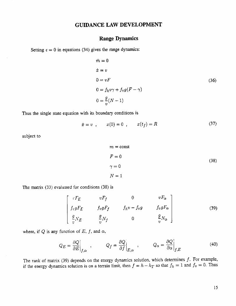
Setting _ = 0 in equations (34) gives the range dynamics:

m=0

0 = vF (36)

o = A73"Y+ fvg(F- "r)

o=g-(N-l)?3

Thus the single state equation with its boundary conditions is

_c = v , x(O) = 0 , x(tf) = R (37)

subject to

m = const

F=O(38)

7=0

N=I

The matrix (33) evaluated for conditions (38) is

uf E vF I 0 vVo_

fcgF E fvgFy fh v -- fvg fvgFa (39)

glvNE v f 0 g-Na, 7d

where, if Q is any function of E, f, and a,

"_ f,o_ -'Of[ OQ] (40)QE-_-OQ , Qy = aQ ' Q_- _ S,EE,o_

The rank of matrix (39) depends on the energy dynamics solution, which determines f. For example,

if the energy dynamics solution is on a terrain limit, then f = h - h T so that fh = 1 and fv = O. Thus

15

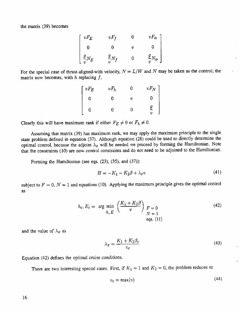
thematrix (39) becomes

_FE vFI 0 _f_

0 0 v 0

g gN v-_NE -i S o g-N_

For the special case of thrust-aligned-with velocity, N = L/W and N may be taken as the control; the

matrix now becomes, with h replacing f,

VFE vFh o _FN

0 0 v 0

g0 0 0 -

V

Clearly this will have maximum rank if either F E ¢ 0 or F h # O.

Assuming that matrix (39) has maximum rank, we may apply the maximum principle to the single

state problem defined in equation (37). Although equation (28) could be used to directly determine the

optimal control, because the adjoint ,kz will be needed we proceed by forming the Hamiltonian. Note

that the constraints (10) are now control constraints and do not need to be adjoined to the Hamiltonian.

Forming the Hamiltonian (see eqs. (23), (35), and (37)):

H = -K1 - K213 + Axv (41)

subject to F = 0, N = 1 and equations (10). Applying the maximum principle gives the optimal control

as

h,E N=I

eqs. (11)

and the value of Az as

Az __ K1 + K2/3c (43)Vc

Equation (42) defines the optimal cruise conditions.

There are two interesting special cases. First, if K1 = 1 and K2 = 0, the problem reduces to

Vc = max(v) (44)

16

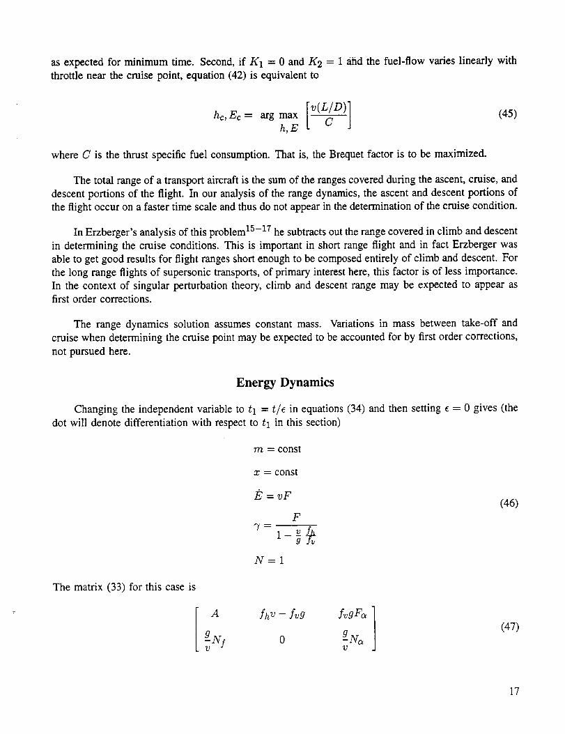
asexpectedfor minimum time. Second,if K1 = 0 and//'2 1 arid the fuel-flow varies linearly with

throttle near the cruise point, equation (42) is equivalent to

hc, Ec= arg max [ L/D IIv(_)]h,E t J

(45)

where C is the thrust specific fuel consumption. That is, the Brequet factor is to be maximized.

The total range of a transport aircraft is the sum of the ranges covered during the ascent, cruise, and

descent portions of the flight. In our analysis of the range dynamics, the ascent and descent portions of

the flight occur on a faster time scale and thus do not appear in the determination of the cruise condition.

In Erzberger's analysis of this problem 15-17 he subtracts out the range covered in climb and descent

in determining the cruise conditions. This is important in short range flight and in fact Erzberger was

able to get good results for flight ranges short enough to be composed entirely of climb and descent. For

the long range flights of supersonic transports, of primary interest here, this factor is of less importance.

In the context of singular perturbation theory, climb and descent range may be expected to appear as

first order corrections.

The range dynamics solution assumes constant mass. Variations in mass between take-off and

cruise when determining the cruise point may be expected to be accounted for by first order corrections,

not pursued here.

Energy Dynamics

Changing the independent variable to tl = t/e in equations (34) and then setting e = 0 gives (the

dot will denote differentiation with respect to tl in this section)

m = const

x = const

E=vF

F7=

N=I

(46)

The matrix (33) for this case is

A

9 Nv i

fhv -

0?j

(47)

17

where

A F [fvg - fhv yah hi f. g + vg fh_ vf f_ + fh vy f. g

--fvh hS g fh v - A_ vs g fh v + fv g (Fh hs + F, vs) (f,, g _ fh _)/F

J

For the case of solution on a terrain limit, f = h - h T , fh = 1, fv = 0, fhh = fvv = fhv = 0 so that

(47) becomes

0 v 0

gN vv _ o _N_

For the special case of thrust-aligned with velocity vector and N replacing a as control, this reduces to

0 v 0

o o g-_3

which is in agreement with Section 6.2 of reference 8, and clearly has maximum rank if v _ 0.

Forming the Hamiltonian associated with equations (46):

H = -K1 - K2,2 + .Xzv + )_EvF (48)

The constraints (10) are state-dependent control constraints for this problem. Maximizing H gives

h=arg max _P)N=I

(49)

hE = const

where

vFp = (5o)

K1 + K2/3 - ,Xzv

with the value of h E as

1

"XE = T (51)

Note that as h and v approach hc and Vc, P becomes infinitely large. The three terms in the denominator

of P have the following obvious interpretation. In climb, three factors are important: minimizing time

(K1 term), minimizing fuel consumption (K2), and covering range (-Azv).

18

For thecaseof anunboundedlocal maximum,equation(49) implies

=0E

or, in terms of v and h (see eqs. (5)),

(52)

For this case,

y(v,h) = P_- v--Phg

"t}

fh = Pvh- _Vhh

1 v

Substituting into the third of equations (46),

F

"7 = v(gPvh--VPhh) (53)1 + g(VPvh+Ph_gpvv)

As mentioned earlier, it is probably best to avoid computing numerical second derivatives and use

equation (18):

F'7-

instead for the value of '7 along the energy dynamics solution.

Fast States Dynamics

Changing the independent variable to t2 = t/e 2 in equations (34) and then setting e = 0 gives (dot

denotes differentiation with respect to t2):

m = const.

x = const.

E = const. (54)

] = YhV7 + fvg(F- "7)

_/= _(N-_)

19

Our main interestin this paperis to use theseequationsto model the altitudetransitionthat typicallyoccurstransonically in the energydynamicssolution for supersonicaircraft. Therehave beenthreeapproachesto the solutionof equations(54).

Ardema7,8for the caseof f = h, left h and "7 on the same time scale and iteratively solved the

associated 2PBVP. Although this is not the approach that will be used here, the problem is formulated

in general in Appendix C as a starting point for future investigation. Calise 33'34 time-scaled decoupled

h and '7 and obtained non-iterative solutions for each. This required adding a penalty term on "7 to the

cost function and a "constrained matching" technique.

The approach used in this paper is a non-optimal one that assumes the fast state dynamics occur

at constant load factor, N. This is motivated by reference 22 which showed that the transonic altitude

transitions occurring in discontinuous energy dynamics solutions consisted of a push-over followed by

a push-up (see fig. 2 which is reproduced from ref. 22). Reference 12 modeled this load factor history

by two constant load factor segments and obtained good results. Using a non-optimal approach to the

fast dynamics is partially justified by the fact that these altitude transitions take relatively little time and

consume relatively little fuel.

One way to approximate the altitude transition is to begin flying a constant minimum load factor

flight path when a jump is detected and then switch to a constant maximum load factor when the new

branch is crossed; this is the dotted path in figure 3, from reference 12. This is undesirable for two

reasons. First, the transition is initiated too late, and second, the transition path overshoots the new

branch of the energy dynamics solution. In our approach, we use the fast state dynamics to determine

_, the optimum point for transition through E (see fig. 3).

Noting that F = 0 because/_ = 0, consider the last two of equations (54)

] = fhv"7- fvg"7

gK

I1

(55)

where K = N - 1 is a known constant.

Following reference 12, the first of these equations is divided by the second to give an equation in

f and "7:

df 11-- = - fvg)"7d7 g/t

df (56)

From equation (9) for E = const., dh = -V--dv so thatg

d11

2O

Substitutinginto equation(56)andcarryingout the integrationgives

_ = _,d_+const.V

1 2-K in v = _3' + const.

(57)

Now label the last point on the subsonic climb path as point 1, the first point on the supersonic

climb path as point 2, and the load factor transition point by an overbar (see fig. 3). Then equation (57)

must hold from point 1 to the transition point with K1 = N1 - 1 and from the transition to point 2 with

K2 =N2-1:

VA 1

-K1 In -_1 = 2 "._2 _ 7i')_'_

_K21nV2 1(2 2)---7 -7v A 2

Solving for _ and 7:

V A =

1

- (58)

_A = t 2(K1"7_ - K2_l 2) + 4K1K2 In v_2(K1 - K2)

This is the same solution as obtained in reference 12 except that now the values of '71 and ")'2 are to be

determined according to equation (15).

The transition path is then determined as follows. Constant load factor solutions are generated with

load factor N1 (see Appendix B) which leave the lower energy branch of the climb path at different

points. The solution that just achieves v = _ when E = E is chosen and then the load factor is set to

N2 for the transition from E to the higher energy branch.

It is also possible to obtain an integrated solution if the small "7 assumption is not made (this was

not possible in reference 12 because of Coriolis and Earth curvature terms). This may be of importance

because 7 may become large in some altitude transitions. Now divide the last two of equations (17)

21

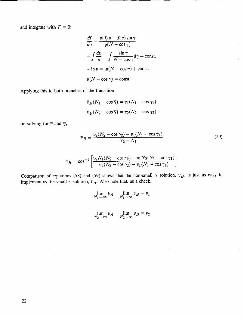
and integratewith F = 0:

df v(fh v - fvg)sin7

d7 g(N - cos 3')

f dv f sin 7 d")' + const.v N - cos 7

- In v = ln(N - cos 7) + const.

v(N - cos 7) = const.

Applying this to both branches of the transition

_B (Yl - cos _) -- Vl (N1 - cos 71)

VB(N2 - cos_) = v2(N2- cos72)

or, solving for V and 7,

v2(N2 - cos_'2)- vl (Arx- cos71)vB= N2-N_

(59)

v2_,v_(At2- cos-_2)- ,-,_N2(_..cos ._)]_B = cos-1 v2(N2 cos72) - vl(N1 - cosT1) j

Comparison of equations (58) and (59) shows that the non-small 7 solution, _B, is just as easy to

implement as the small ":. solution, YA- Also note that, as a check,

lira VA= lira VB=Vl:V1 ---.r_ N1 ----*oo

lim VA = lira VB = v2N2---,cc N2---,_

22

NUMERICAL EXAMPLE

The guidance algorithm developed in the previous section has been implemented in the ACSYNT

Computer Code and used to compute near-optimal trajectories for a supersonic transport design. The

main characteristics of the design are listed in table 1.

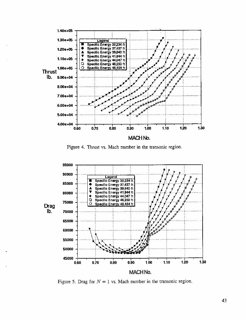
Figure 4 shows maximum thrust of the aircraft as a function of Mach number for various energy

levels (recall that a linear throttle is not assumed), and figure 5 shows the total drag for N = 1 as a

function of Mach for various energy levels, in the region of Mach 1. The transonic drag rise is clearly

shown in figure 5, and this raises the possibility that there may be an instantaneous altitude transition

in the energy climb path near Mach 1.

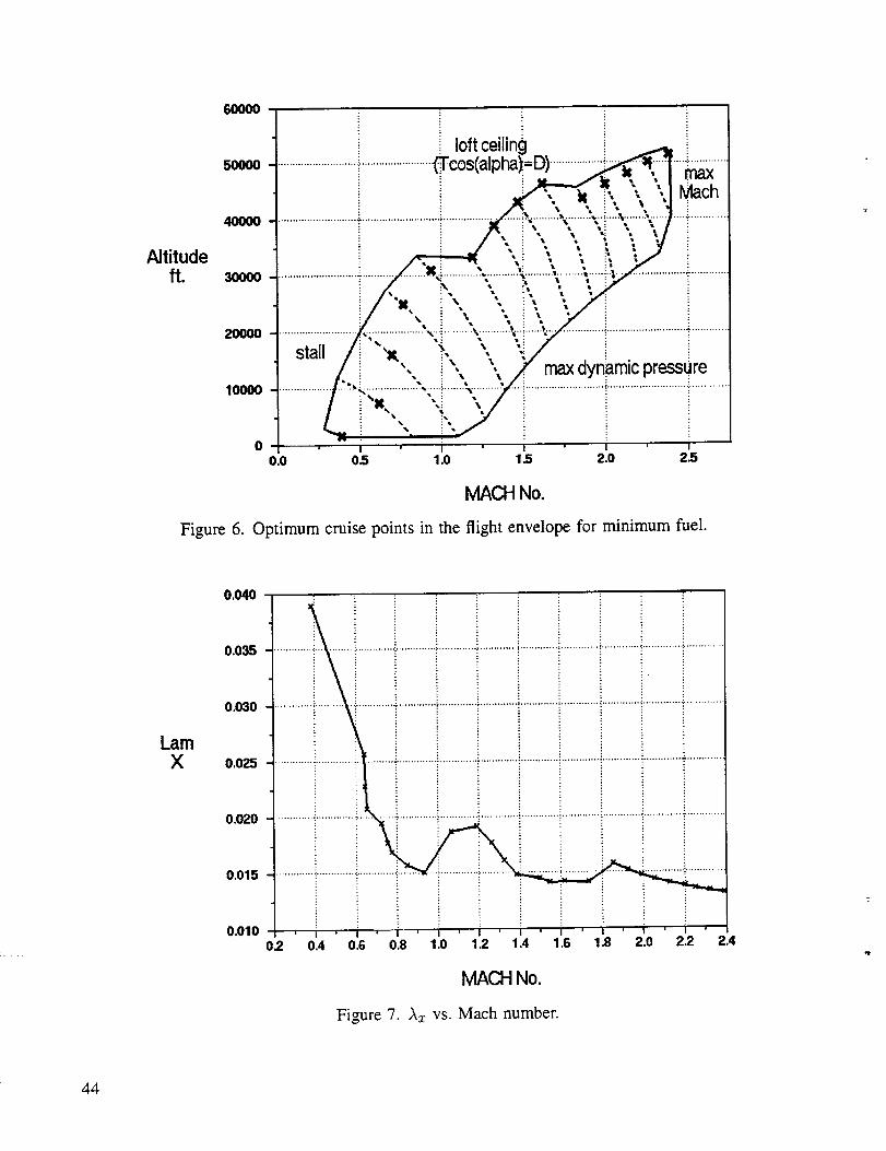
The first step of the algorithm is to find the optimum cruise point, as given by equation (42). Figure 6

shows the optimal cruise point at each energy level throughout the flight envelope for minimum fuel

(K1 = 0 and K2 = 1). The optimal cruise point is interior to the flight envelope except from about

Mach 1.25 to Mach 1.75, for which it is on the loft ceiling bound.

Figure 7 shows the data of figure 6 plotted in a different way, as ,kz vs. Mach (see eq. (43)). This

curve has three local minimums, each a locally optimal cruise point. One of these is a subsonic condition

at Mach 0.95. The globally optimum point is at Mach 2.4, the highest Mach allowed. From figure 6,

this Mach 2.4 cruise point is at an altitude of about 52,500 ft. The Mach 2.4 cruise condition has about

a 15% higher cruise efficiency than the Mach 0.95 condition, as measured by Az; the Mach 0.95 cruise

point would be used for over-land flight.

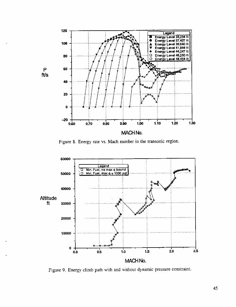
The next step in the algorithm is determining the climb path. This involves maximizing P (see

eqs. (49) and (50)) with respect to h at energy levels from take-off to cruise. Figure 8 plots P as a

function of Mach for various energy levels for maximum thrust and again minimum fuel. The maximum

dynamic pressure constraint is not applied for this calculation. The value of Az used in equation (50) is

given by equation (43) for the Mach 2.4 optimal cruise condition. It is seen that for many energy levels

P has two or more local maxima in the vicinity of Mach 1; it is the jumping of the global maxima

between these local maxima that causes the transonic altitude transition.

The resulting flight path in the Mach-altitude plane is shown in figure 9. The path starts along a

terrain limit and then climbs at almost a constant high subsonic Mach. At about 32,500 ft, it instan-

taneously transitions to about 22,500 ft at Mach 1.25. It then continues up to the cruise point, with

a jump to higher altitudes between Mach 1.6 and 1.8. Also shown in figure 9 is the path with the

dynamic pressure constraint imposed. It is seen that the unconstrained path violates the constraint by

only a small amount between Mach 1.3 and 1.7.

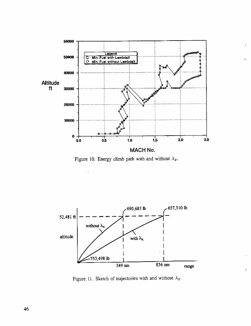
Figure 10 compares the minimum fuel flight path with Az included in P in equation (50) with the

path with the Az term omitted. The latter case corresponds to minimum fuel to climb without regard to

a range constraint. The paths are similar except at high speed where the path with Az omitted has much

higher dynamic pressure (there is no dynamic pressure constraint imposed). A computation was made

to verify that including the Az term gives better performance. Referring to figure 11, the path with the

Az term included ended with an airplane weight of 657,310 lb and a range of 836 nm. The path without

Az ended at 690,683 Ib and 349 nm. By the Brequet formula, the range covered in a cruise condition

23

is (seeeq. (45)):

v(L/D) In m0c

At the cruise condition, v = 2323 ft/sec, (L/D) = 9.0, and C' = 1.315 lbfuel per hour per lbthrust. Thus

for the same fuel consumed along the path with Az, the path without Az, has a range of

(9.0)(2323) (3600'_ In 690,683 _ 815 nm349+ (1.315) \6076} 657,310

Thus the case with Az gives 21 nm. more range for the same fuelthan the case without Az.

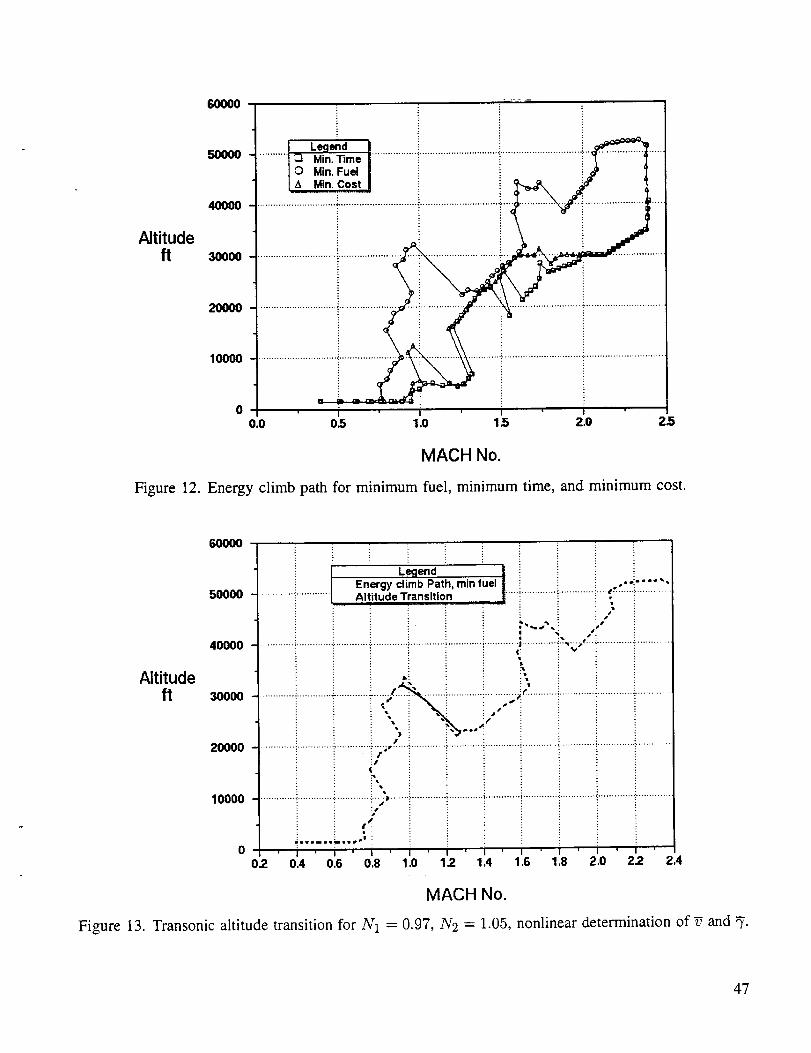
Minimum fuel, minimum time (K1 = 0, /'/2 = 1), and "minimum direct operating cost" climb

trajectories are compared in figure 12. For the minimum cost trajectory, K1 = $500/hr and K2 =

$0.0626/lb; these are the values used in reference 15 for short range subsonic transports, and would

likely need to be adjusted for supersonic long range transports. The minimum fuel and minimum time

trajectories are quite different. The latter has no transonic altitude transition, whereas the former has

a large one. Also, the minimum time path is much lower in altitude in the high supersonic range (the

dynamic pressure constraint was relaxed for this calculation and would be violated by the minimum

time path). As expected, the minimum cost path is intermediate between the other two, being more like

the minimum time path.

One of the principal goals of this research has been to develop an algorithm for computing the

trajectory segments connecting the branches of the energy climb path in the transonic region, that is,

the altitude transitions. Specifically, equation (50) was used to determine _, the value of v which is to

be obtained when E = "E (see fig. 3). An iteration is then made to determine where on the subsonic

branch of the ECP the departure should be made to achieve this condition. The constant load factor

integration as described in Appendix B is used to generate the flight paths.

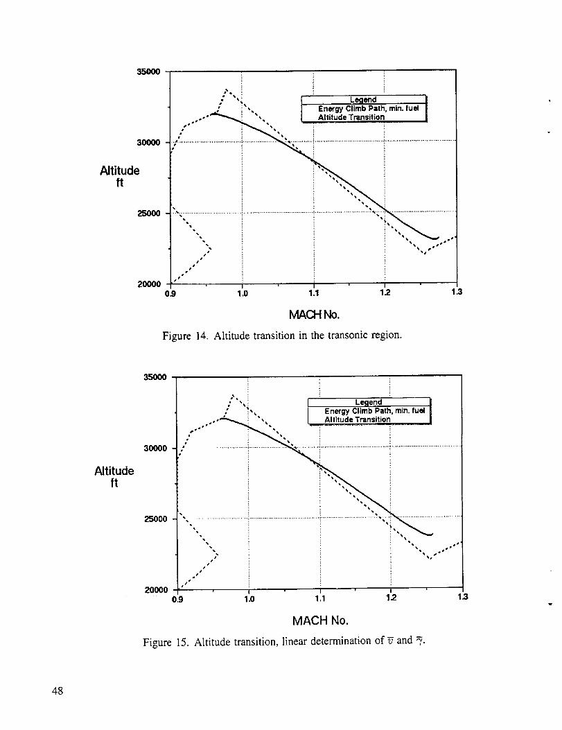
Figure 13 shows the transition for N1 = 0.97 and N2 = 1.05 for the minimum fuel case in the

altitude-Mach plane, and figure 14 shows the same path in the transonic region. The integration is

terminated when the flight path angle is equal to the flight path angle on the supersonic branch of the

ECP as given by equation (53). The dynamic pressure limit was ignored for this calculation. The figures

show that there is a very close match between the altitude transition and the ECP at the termination of

the former, and that even mild maneuvers (N1 and N2 close to 1) give adequate transition trajectories.

The transition trajectories for the same conditions, but using the linear estimate of g as given by

equation (58), are shown in figure 15. Comparing figures 14 and 15 shows that the nonlinear solution

gives a better match with the supersonic branch of the ECP than does the linear.

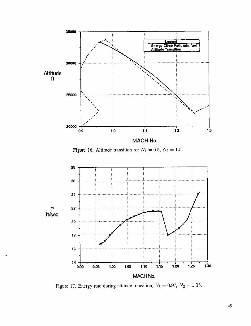
The transition trajectory for a more severe load factor maneuver, N1 = 0.5 and N2 = 1.5, is shown

in figure 16 (these load factors would not be acceptable for a commercial transport). As compared with

a more benign maneuver, as shown in figure 14, the transition through E occurs at a much higher

altitude and the trajectory is much closer to E, as expected.

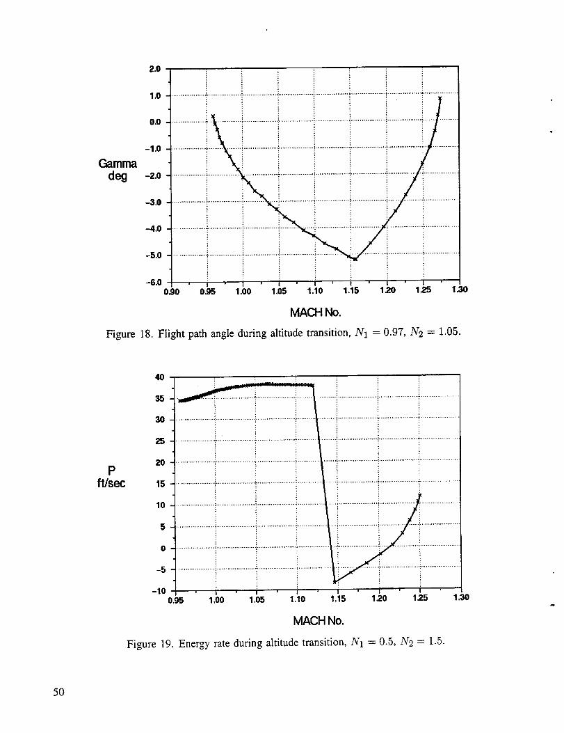
Figure 17 shows the variation of energy rate, vF, as a function of Mach in the transonic region for

the mild transition (N1 = 0.97, IV2 = 1.05). As expected, the energy rate drops when the load factor is

24

switchedfrom 0.97 to 1.05,but nevergetsnearzero. Also asexpected,theflight pathangle,7, at firstdecreases,and thenincreaseswhentheloadfactor is switchedasshownin figure 18; themagnitudeof"7staysbelow 6 deg,makingthesmall "7 approximation extremely good.

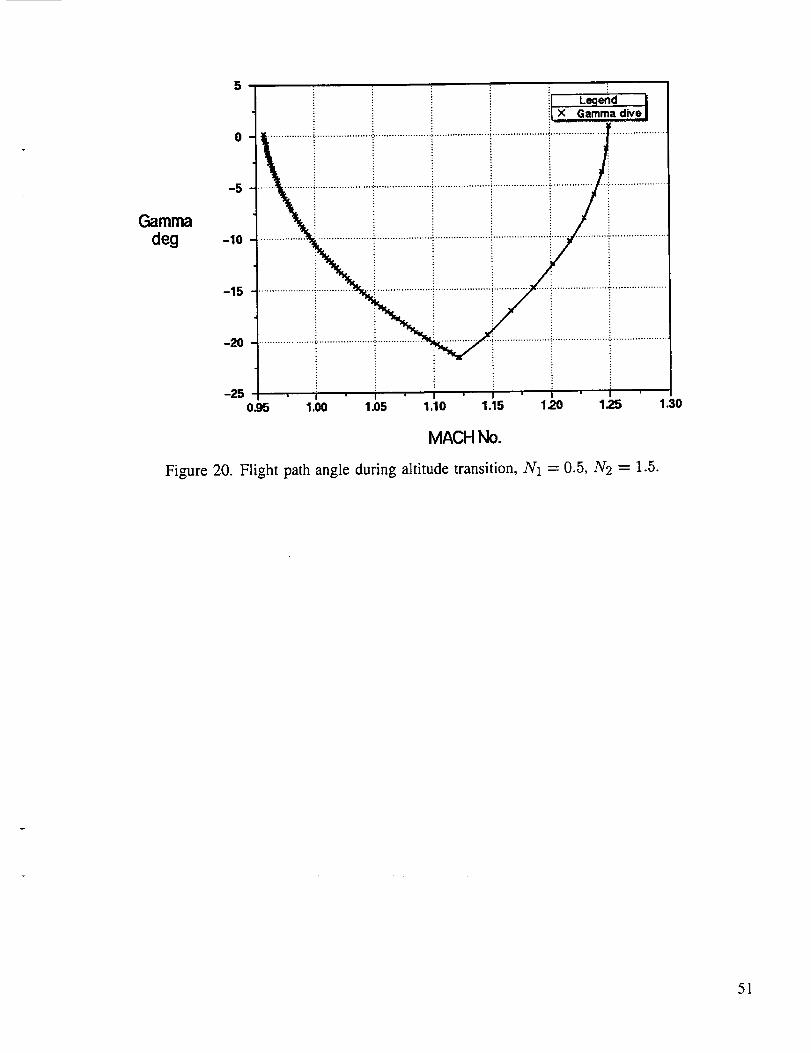
The same plots are made for the more severe maneuver (N 1 = 0.5, N 2 = 1.5) in figures 19 and

20. In this case, the energy rate becomes negative after the load factor switch and the magnitude of

"7 reaches about 22 deg, meaning that equations (59) and not equations (58) should be used for the

calculation of the transition point.

25

CONCLUDING REMARKS

An algorithm for optimizing supersonic transport trajectories suitable for use in an aircraft synthesis

computer code has been developed. The algorithm has been implemented in the ACSYNT computer

program and illustrated using a typical supersonic transport design.

The algorithm is based on singular perturbation theory and complete time-scale decoupling of the

energy-state version of the equations of motion (except for the fast dynamics). This results in replacing

the functional optimization problem by a series of function optimization problems.

The first problem is determining the optimal cruise condition. This involves a weighted sum of

the importance of time and fuel consumption. The second problem is determining the energy-climb

path (ECP) to the cruise condition, which involves a weighted sum of the importance of time, fuel

consumption, and cruise efficiency.

For the fast dynamics, a variable is introduced such that the ECP gives a consistent value of the

flight path angle. This variable is left on the same time scale as the flight path angle and a nonoptimal

solution of the fast dynamics using constant load factor segments is obtained.

Numerical results for a nominal supersonic transport showed the following: (1) The optimal cruise

point was at the highest and fastest point in the flight envelope, although there are local optimal cruise

points at high subsonic and low supersonic speeds. (2) The ECP for the minimum fuel case had a largetransonic altitude transition, the minimum time case had no transition, and the minimum direct operating

cost case had a mild transition. (3) The altitude transition solutions gave good matches between the

subsonic and supersonic branches of the ECP with operationally acceptable load factors.

There are two obvious shortcomings of the present state of the analysis. First, the weight is

held constant during the search for the optimal cruise point. This weight is the gross take-off weight

according to the time-scale assumptions, but in practice could be some empirical estimate of the weight

at the start of cruise. Second, the range during climb and descent is ignored when optimizing the cruise

point. This is obviously a more serious problem at short ranges than for the long ranges of a supersonic

transport.

It is expected that both of these shortcomings could be eliminated by solving the time-scaled

equations of motion to first order, that is, by expanding all the state variables to first order terms. This

is the next obvious step in this research. In addition to solving these problems, the first order solutions

will give better overall accuracy to the algorithm.

26

APPENDIX A - NOMENCLATURE

D = drag

E = mechanical energy

F = normalized tangential force

g = gravity

h = altitude

H = Hamiltonian

d = cost functional

L = lift

m = mass

M = Mach number

q = dynamic pressureT = thrust

v = velocity

z = range

a = angle of attack

/3 = fuel flow rate

c = small parameter

7 = flight path angle

A = adjoint variable

_b = cost function

p = air density

27

APPENDIX B - NUMERICAL INTEGRATION OF STATE EQUATIONS

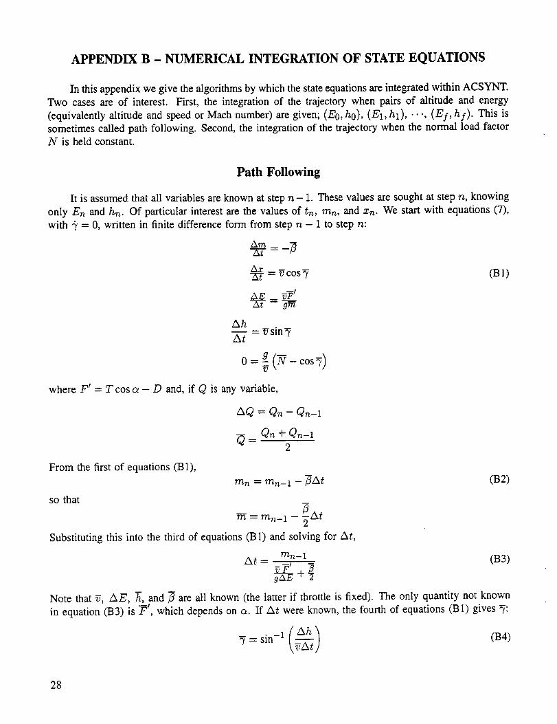
In this appendix we give the algorithms by which the state equations are integrated within ACSYNT.

Two cases are of interest. First, the integration of the trajectory when pairs of altitude and energy

(equivalently altitude and speed or Mach number) are given; (E0, h0), (El, hl), " ", (El, hy). This is

sometimes called path following. Second, the integration of the trajectory when the normal load factor

N is held constant.

Path Following

It is assumed that all variables are known at step n- 1. These values are sought at step n, knowing

only En and hn. Of particular interest are the values of tn, ran, and Xn. We start with equations (7),

with + = 0, written in finite difference form from step n - 1 to step n:

Am--A-T= -_

Az = _COS_ 031)'h-'f

AE _'-_-T = g---_-

Ah= _sin_

At

o= co v)V

where F I = T cos a - D and, if Q is any variable,

nQ = On - Qn-1

Qn + Qn-1Q=

2

From the first of equations (B 1),

mn = ran-1 - -_At

so that¢9

= ran-1 -- -_At

(B2)

Substituting this into the third of equations 031) and solving for At,

At = ran-1 033)

Note that g, AE, -h, and _ are all known (the latter if throttle is fixed). The only quantity not known

in equation 033) is F, which depends on a. If At were known, the fourth of equations 031) gives "7:

= sin_ 1 ( _xh '] (B4)\FET]

28

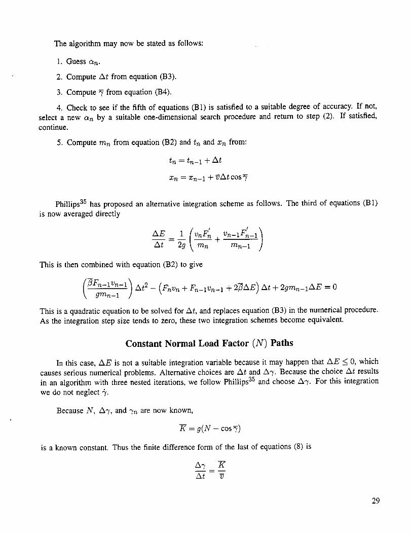
Thealgorithmmay now be statedasfollows:

1. Guessan.

2. Compute At from equation 033).

3. Compute _ from equation 034).

4. Check to see if the fifth of equations 031) is satisfied to a suitable degree of accuracy. If not,

select a new an by a suitable one-dimensional search procedure and return to step (2). If satisfied,

continue.

5. Compute mn from equation 032) and tn and Xn from:

tn = tn-1 + At

Xn = Xn-1 + _Atcos_

Phillips 35 has proposed an alternative integration scheme as follows. The third of equations (B 1)

is now averaged directly

AE 1 + Vn-lFn_ 1

At 29 \ mn ran-1

This is then combined with equation 032) to give

This is a quadratic equation to be solved for At, and replaces equation (B3) in the numerical procedure.

As the integration step size tends to Zero, these two integration schemes become equivalent.

Constant Normal Load Factor (N) Paths

In this case, AE is not a suitable integration variable because it may happen that AE _< 0, which

causes serious numerical problems. Alternative choices are At and AT. Because the choice At results

in an algorithm with three nested iterations, we follow Phillips 35 and choose A,,/. For this integration

we do not neglect _'.

Because N, A,,/, and ";'n are now known,

-K = g( N - cos 7)

is a known constant. Thus the finite difference form of the last of equations (8) is

w

A? K

At g

29

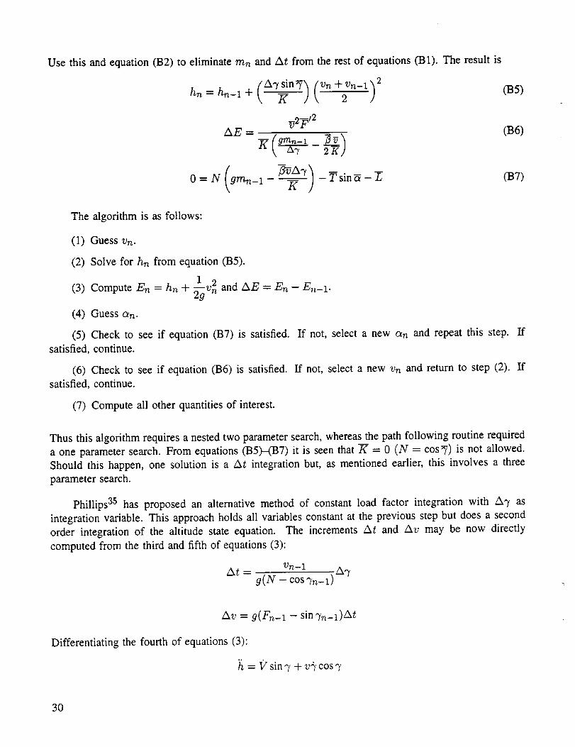
Use this andequation032) to eliminate mn and At from the rest of equations 031). The result is

hn = hn_l + (ATs__._n') (Vn +2n-1)2 (B5)

AE = (B6)

The algorithm is as follows:

(1) Guess Vn.

(2) Solve for hn from equation 035).

(3) ComputeEn=hn+ 1 2 andAE En En-12-..-_v n -- _ .

(4) Guess an.

(5) Check to see if equation 037) is satisfied. If not, select a new an and repeat this step.

satisfied, continue.

(6) Check to see if equation 036) is satisfied. If not, select a new Vn and return to step (2).

satisfied, continue.

(7) Compute all other quantities of interest.

If

If

Thus this algorithm requires a nested two parameter search, whereas the path following routine required

a one parameter search. From equations 035)-037) it is seen that K = 0 (N = cos 7) is not allowed.

Should this happen, one solution is a At integration but, as mentioned earlier, this involves a three

parameter search.

Phillips 35 has proposed an alternative method of constant load factor integration with A,y as

integration variable. This approach holds all variables constant at the previous step but does a second

order integration of the altitude state equation. The increments At and Av may be now directly

computed from the third and fifth of equations (3):

Vn-1 A,,/At = g(N - cos%_l)

Av = g(Fn-1 - sin'Yn-1) At

Differentiating the fourth of equations (3):

= l_ sin "/+ v'}' cos "/

30

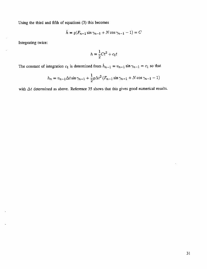
Usingthe third and fifth of equations(3) this becomes

h = 9(Fn_l sin")'n-1 + NcosTn-1 - 1) = C

Integrating twice:

= 1Ct2 + Cl th

The constant of integration Cl is determined from _tn_ 1 -- vn_ 1 sin _'n-1 = Cl SO that

1 2hn = Vn-lAtsin_/n-1 + _gAt (Fn-1 sin"fn-1 + Ncos_'n-1 - 1)

with At determined as above. Reference 35 shows that this gives good numerical results.

31

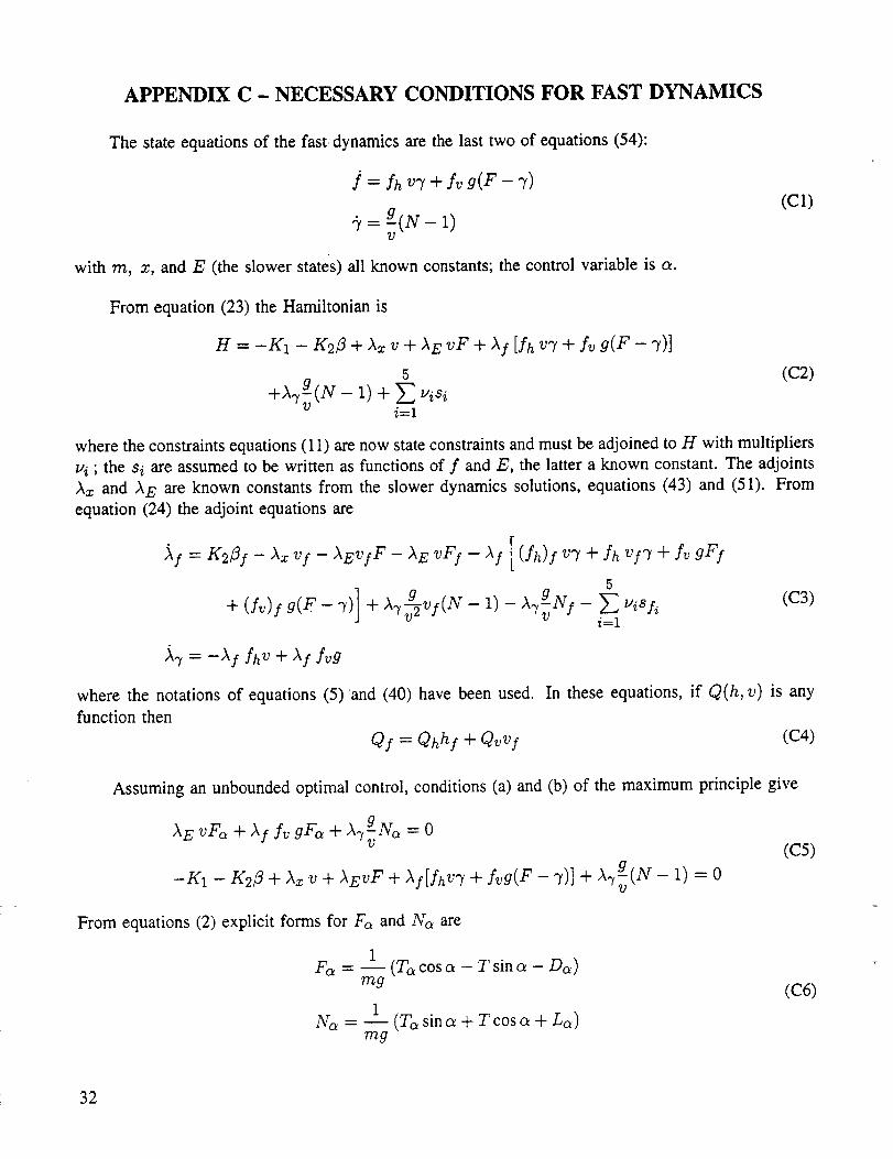
APPENDIX C - NECESSARY CONDITIONS FOR FAST DYNAMICS

The state equations of the fast-dynamics are the last two of equations (54):

1 = A v7 + Yvg(F- 7)

-_ = g-(N- 1)v

with m, x, and E (the slower states) all known constants; the control variable is a.

(C1)

From equation (23) the Hamiltonian is

H = -K: - K2_ + )_z v + AEvF + Af [fh v7 + fv g(F - 7)]

5

i=1

(C2)

where the constraints equations (1 i) are now state constraints and must be adjoined to H with multipliers

vi ; the si are assumed to be written as functions of f and E, the latter a known constant. The adjoints

Az and AE are known constants from the slower dynamics solutions, equations (43) and (51). From

equation (24) the adjoint equations are

A f = K2j3f - Az vf - AEvfF- )_EVFZ - A f [ (fh)fV7 + fh v f7 + fv gFy

5(C3)

_7 = -Af fh v + Af fvg

where the notations of equations (5)and (40) have been used.

function then

Qf = Qhhf + Qvvf

In these equations, if Q(h, v) is any

(C4)

Assuming an unbounded optimal control, conditions (a) and (b) of the maximum principle give

-K: - K2/3 + ikz v + AEVF + Af[fhv7 + fvg(F -7)] + A'rg( N- 1) = 0

(C5)

From equations (2) explicit forms for Fa and Na are

1F_-

mg- -- (Ta cos a - T sin a - Da)

1_h_ = u (Ta sin a + T cos a + La)

mg

(C6)

32

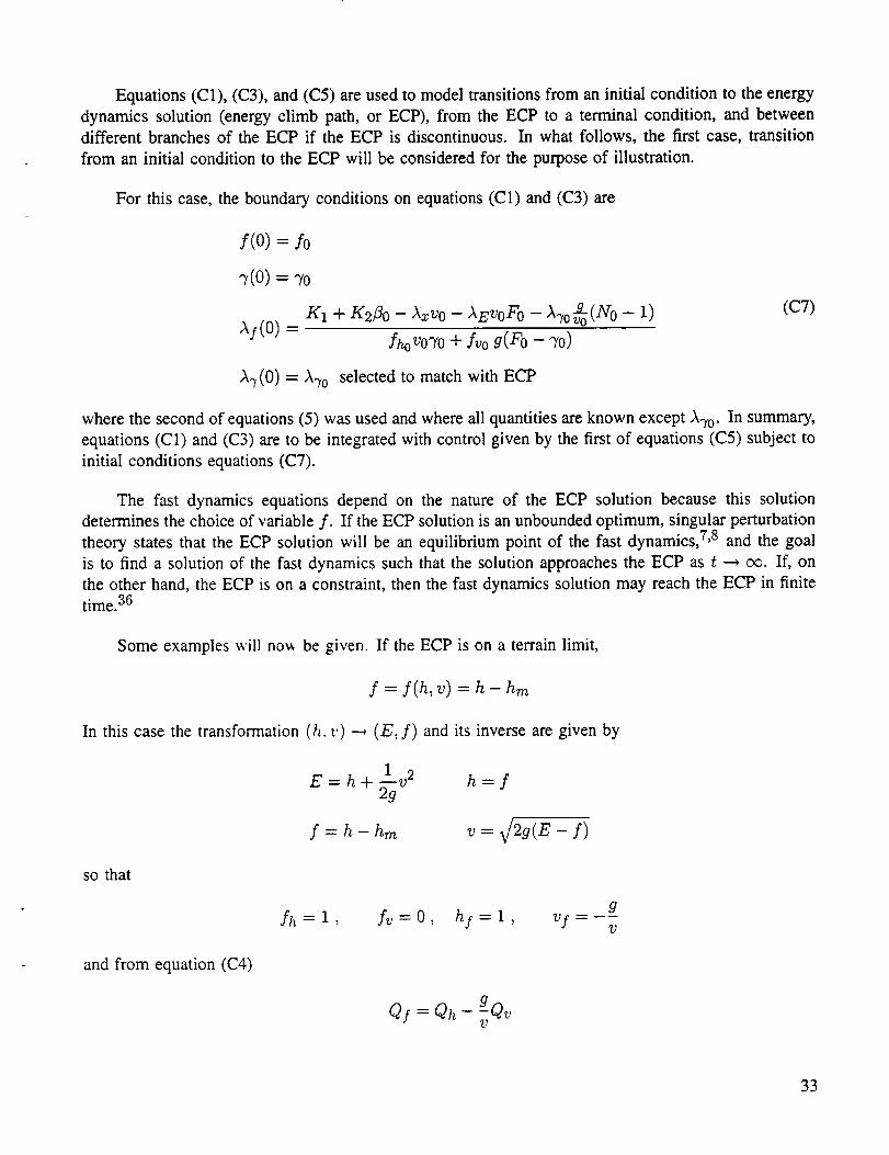
Equations(C1), (C3),and(C5) areusedto modeltransitionsfrom aninitial condition to theenergydynamicssolution (energyclimb path, or ECP), from the ECP to a terminalcondition, and betweendifferent branchesof the ECP if the ECP is discontinuous.In what follows, the first case,transitionfrom an initial conditionto the ECPwill be consideredfor the purposeof illustration.

For this case,theboundaryconditionson equations(C1) and(C3) are

/(o) =/o

-_(o): "_o

K1 + K2#0 - Azvo- AEvoFo- ATo_(No- 1)_:(o) =

AoVO'yO+ Ao g(Fo -_o)

A._(0) = A-r0 selected to match with ECP

(C7)

where the second of equations (5) was used and where all quantities are known except _'_o. In summary,

equations (C1) and (C3) are to be integrated with control given by the first of equations (C5) subject to

initial conditions equations (C7).

The fast dynamics equations depend on the nature of the ECP solution because this solution

determines the choice of variable f. If the ECP solution is an unbounded optimum, singular perturbation

theory states that the ECP solution will be an equilibrium point of the fast dynamics, 7,8 and the goal

is to find a solution of the fast dynamics such that the solution approaches the ECP as t _ oc. If, on

the other hand, the ECP is on a constraint, then the fast dynamics solution may reach the ECP in finitetime. 36

Some examples will nov, be given. If the ECP is on a terrain limit,

f = y(h, v) = h - hm

In this case the transformation (h. v) ---, (E, f) and its inverse are given by

1 2

E=h+_gV

f=h-hm

so that

gfh = l, fv=O, h/= l, vf =--

U

and from equation (C4)

Q.f = Qh - g-QvV

33

Putting theseresultsinto equations(C1) and(C3)

]=V'y

,_= g(N-1)v

,_, = -Afv

and into equations (C5)

+ )_TgN_ = 0AEvFa

-K1 - K2_ + AxV + AEvF + Afv.,/ + A-rg(N 1) 0

The initial conditions for the integration of equations (C7) are as follows:

f(O) = fo

-y(o)= "_o

K1 +//'2/30 - Azvo - AEvOFO - ATo g(N0 - 1)v_j(o) =vO'YO

A.;,(O) = A_,o , selected to match with ECP

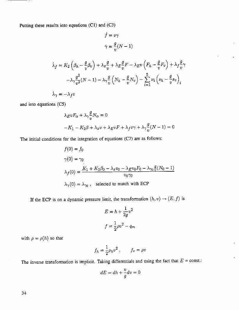
If the ECP is on a dynamic pressure limit, the transformation (h, v) ---* (E, f) is

E=h+lv 22g

1 2f= _ -qm

with p = p(h) so that

1h = :ph v2 L = p_

2

The inverse transformation is implicit. Taking differentials and using the fact that E = const.:

dE = dh + V dv = 0g

34

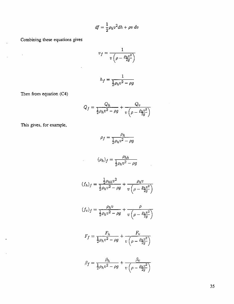
Combining these equations gives

1 2elf = -_ph v dh + pv dv

_'-v(___)

Then from equation (C4)

This gives, for example,

1

hf = ½PhV 2 _ Pg

Qh Qv

Ph

pf = ½PhV2 -- pg

l p v 2hh Ph v= +

. Ph v + P

Fh+

Zh Zv+_: _v___ v(___)

35

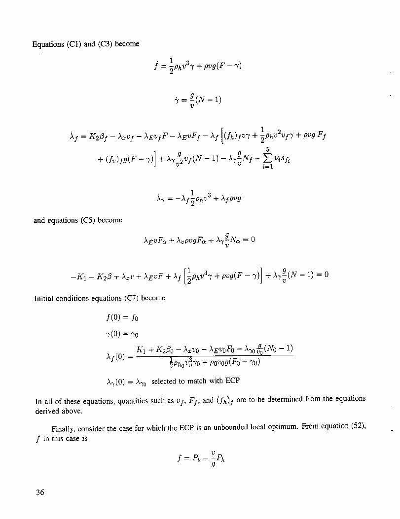
Equations (C1) and (C3) become

1 3

g-_= v(N-1)

5

and equations (C5) become

1 3

_'7 -- --/_f_Ph v + Afpvg

),E.vF_ + AvpvgF,_+ A.ygNo, = 0

f1 3 + pvg(F-'7)]+ g - 1) 0

Initial conditions equations (C7) become

f(O) = fo

:,(0)= ;.o

h'l + K2_o - A_vo- AE,voFo - A-yo_(No - l)A f(0)

_pho@YO+ povog(Fo- "yo)

AT(0) = _70 selected to match with ECP

In all of these equations, quantities such as v f, Ff, and (fh)f are to be determined from the equations

derived above.

Finally, consider the case for which the ECP is an unbounded local optimum. From equation (52),

f in this case is

f=Pv-v-Phg

36

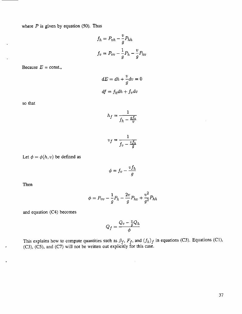
where 19 is given by equation (50). Thus

Because E = const.,

so that

q_

.fh= Pvh - _Phh

1 v

Iv- - - Shv

dE = dh + V dv = 0g

df = fhdh + fvdv

1

vf = _ _ __&g

Let ¢ = ¢(h, v) be defined as

_fh¢=f_---

g

Then

1 2Vp v 2¢ = Pvv -- gPh - g hv +-_Phh

and equation (C4) becomes

This explains how to compute quantities such as fly, Fy, and (fh)f in equations (C3). Equations (C1),

(C3), (C5), and (C7) will not be written out explicitly for this case.

37

REFERENCES

1. Myklebust, Arvid; and Gelhausen, P.: Putting the ACSYNT on Aircraft Design. Aerospace

America, Sept. 1994, pp. 26-30.

2. Calise, A.: Singular Perturbation Methods for Variational Problems in Aircraft Flight. IEEE

Transactions on Automatic Control, vol. AC-21, June 1976, pp. 345-353.

3. Calise, A.: Extended Energy Management Methods for Flight Performance Optimization. AIAA

Journal, vol. 15, no. 3, Mar. 1977, pp. 314-321.

4. Calise, A.: A New Boundary Layer Matching Procedure for Singularly Perturbed Systems.

IEEE Transaction on Automatic Control, vol. AC-23, no. 3, June 1978.

5. Kelley, H.: Aircraft Maneuver Optimization by Reduced-Order Approximation. Control and

Dynamic Systems, vol. 10, Academic Press, New York, 1973, pp. 131-178.

6. Kelley, H.; and Edelbaum, T.: Energy Climbs, Energy Turns, and Asymptotic Expansions.

Journal of Aircraft, vol. 7, Jan. 1970, pp. 93-95.

7. Ardema, M.: Solution of the Minimum Time-to-Climb Problem by Matched Asymptotic Expan-

sions. AIAA Journal, vol. 14, no. 7, July 1976.

8. Ardema, M.: Singular Perturbations in Flight Mechanics. NASA TM X-62,380, Aug. 1974.

9. Shinar, J.: On Applications of Singular Perturbation Techniques in Nonlinear Optimal Control.

Automatica, vol. 19, no. 2, 1983, pp. 203-211.

10. Bryson, A.; Desai, M.; and Hoffman, W.: Energy-State Approximation in Performance Opti-

mization of Supersonic Aircraft. Journal of Aircraft, vol. 6, no. 6, Nov.-Dec. 1969.

11. Kelley, H.; Cliff, E.; and Weston, A.: Energy State Revisited. Optimal Control Applications

& Methods, vol. 7, 1986, pp. 195-200.

12. Ardema, M.; Bowles, J.; Terjesen, E.; and Whittaker T.: Approximate Altitude Transitions for

High-Speed Aircraft. Journal of Guidance, Control, and Dynamics, vol. 18, no. 3, May-June 1995,

pp. 561-566.

13. Ardema, M.; and Rajan, N.: Selection of Slow and Fast Variables in Three-Dimensional Flight

Dynamics. American Control Conference, WP7-3:30, June 1984.

14. Ardema, M.; and Rajan, N.: Slow and Fast State Variables for Three-Dimensional Flight

Dynamics. Journal of Guidance, Control, and Dynamics, vol. 8, no. 4, July-Aug. 1985.

15. Erzberger, H.: Automation of On-Board Flight path Management. NASA TM 84212, Dec.

1981.

16. Erzberger, H.: Theory and Applications of Optimal Control in Aerospace Systems. AGARDo-

graph No. 251, July 1981.

17. Erzberger, H.; and Lee, H.: Algorithm for Fixed-Range Optimal Trajectories. NASA TP 1565,

July 1980.

38

18. Breakwell,J.: Optimal Flight-Path-Angle Transitions in Minimum-_me Airplane Climbs. Jour-

nal of Aircraft, vol. 14, no. 8, Aug. 1977.

19. Breakwell, J.: More about Flight-Path-Angle Transitions in Optimal Airplane Climbs. Journal

of Guidance and Control, vol. 1, no. 3, May-June 1978.

20. Weston, A.; Cliff, E.; and Kelley, H.: Altitude Transitions in Energy Climbs. Automatica,

vol. 19, Mar. 1983, pp. 199-202.

21. Shinar, J.; and Fainstein, V.: Improved Feedback Algorithms for Optimal Maneuvers in Vertical

Plane. AIAA Paper 85-1976, 1985.

22. Ardema, M.; and Yang, L.: Interior Transition Layers in Flight-Path Optimization. Journal of

Guidance, vol. 11, no. 1, Jan.-Feb. 1988.

23. Ardema, M.; and Rajan, N.: Separation of Time Scales in Aircraft Trajectory Optimization.

Journal of Guidance, Control, and Dynamics, vol. 8, no. 2, Mar.-Apr. 1985.

24. Bharadwaj, S.; Wu, M.; and Mease, K.: Identifying Time-Scale Structure for Simplified Guid-

ance Law Development. AIAA Guidance, Navigation, and Control Conference, AIAA Paper 97-3708,

1997.

25. Bryson, A.; and Ho, Y.: Applied Optimal Control. Hemisphere Publishing Co., 1975.

26. Jacobson, E.; Lele, M.; and Speyer, J.: New Necessary Conditions of Optimality for Control

Problems with State-Variable Inequality Constraints. Journal of Mathematical Analysis and Applica-

tions, vol. 35, Aug. 1971, pp. 255-284.

27. Pontryagin, L.; Boltyanskii, U.; Garnkrelidze, R.; and Mishchenko, E.: The Mathematical

Theory of Optimal Processes. Interscience, 1962.

28. Leitmann, G.: The Calculus of Variations and Optimal Control. Plenum Press, New York and

London, 1981.

29. Tihonov, A.: Systems of Differential Equations Containing Small Parameters Multiplying Some

of the Derivatives. Math. Sb., vol. 73, no. 3, N.S. (31), 1952 (in Russian).

30. Vasileva, A.: Asymptotic Behavior of Solutions to Certain Problems Involving Nonlinear Dif-

ferential Equations Containing a Small Parameter Multiplying the Highest Derivatives. Russian Math

Surveys, vol. 18, no. 3, 1963.

31. O'Malley, R.: Introduction to Singular Perturbations: Academic Press, New York and London,

1974.

32. Kokotovic, R; and Sannuti, E: Singular Perturbation Method for Reducing the Model Order

in Optimal Control Design. IEEE Trans. on Automatic Control, vol. 13, no. 4, Aug. 1968.

33. Calise, A.; Aggarwal, R.; and Goldstein, E: Singular Perturbation Analysis of Optimal Flight

Profiles for Transport Aircraft. Joint Automatic Control Conference, June 1977.

34. Calise, A.: Optimization of Aircraft Altitude and Flight-Path Angle Dynamics. Journal of

Guidance, Control and Dynamics, voI. 7, no. 1, Jan.-Feb. 1984.

39

35. Phillips, J.: An Accurate and Flexible Trajectory Analysis. Paper 975599, presented at the

1997 World Aviation Congress, Anaheim, CA, Oct. 1997.

36. Calise, A.; and Corban, J.: Optimal Control of Two-Time-Scale Systems with State-Variable

Inequality Constraints. Journal of Guidance, Control, and Dynamics, voI. 15, no. 2, Mar.-Apr. 1992.

4O

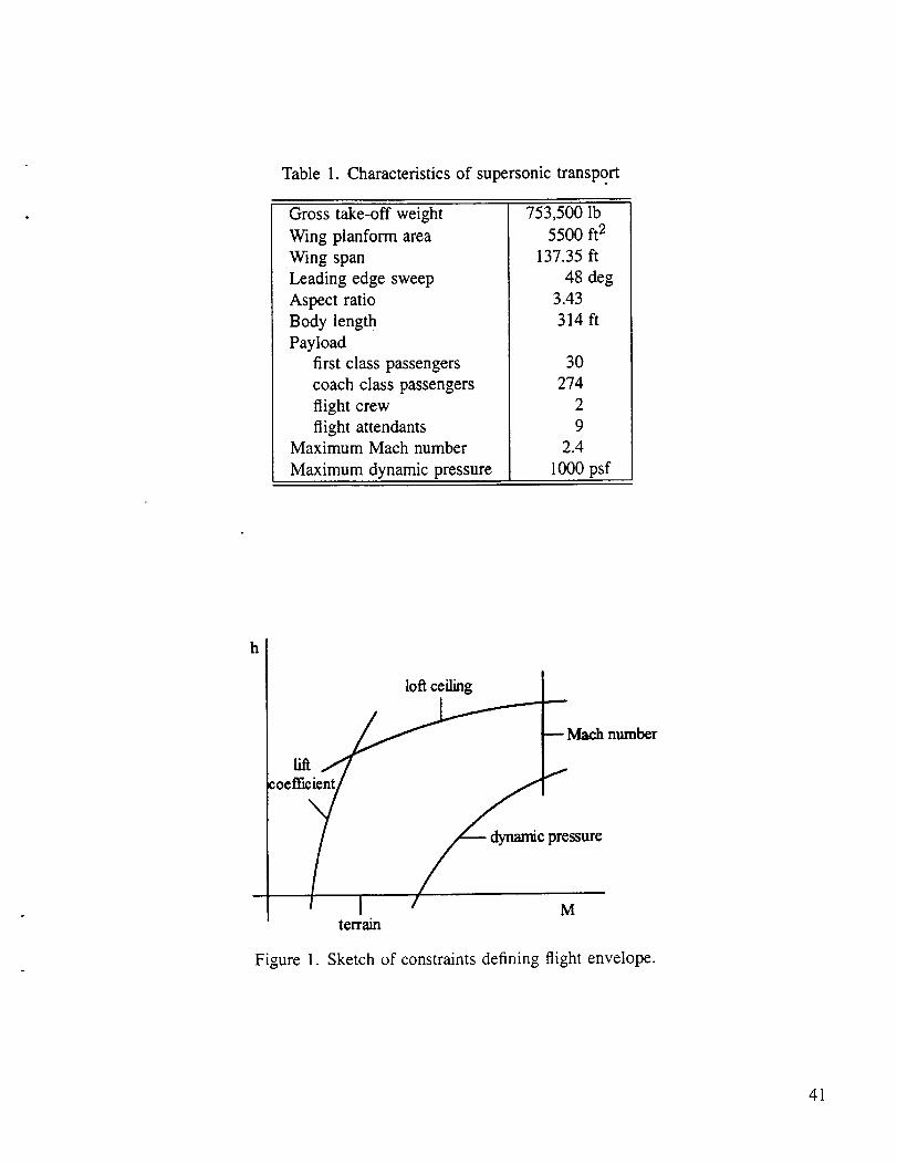
Table1. Characteristicsof supersonictransport

Grosstake-off weightWing planformareaWing spanLeadingedgesweepAspectratioBody lengthPayload

first classpassengerscoachclasspassengersflight crewflight attendants

Maximum MachnumberMaximum dynamicpressure

753,500Ib5500ft2

137.35ft48 deg

3.43314ft

30274

29

2.41000psf

h

loftceiling

lift:oeffici

¢ _ dynamic pressure

/I M

Figure 1.

terrain

Sketch of constraints defining flight envelope.

41

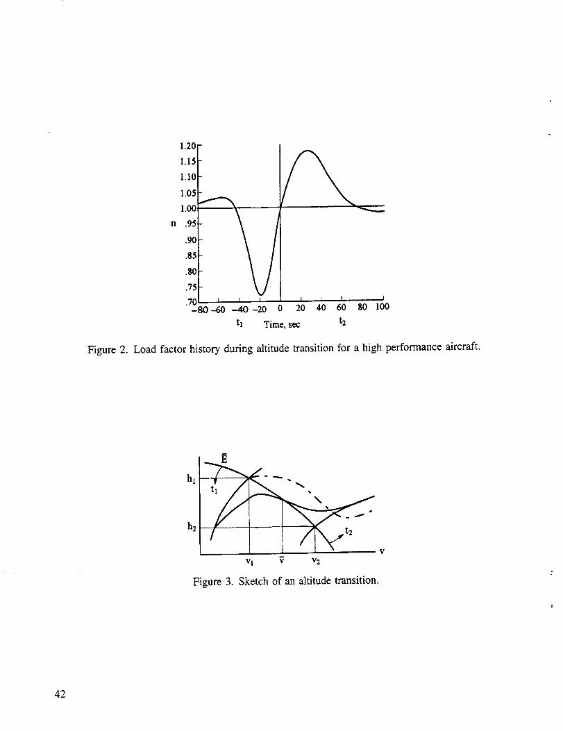
Figure 2.

n

1.20

1.15

1.10

1.05

1.00

.95

.90

.85

.80

.75

.70 I v-80 -60 -40 -20 0

tl

I I 1 J

20 40 60 80 100

Time, se¢ t2

Load factor history during altitude transition for a high performance aircraft.

hi

h2/

Figure 3.

v V v2

Sketch of an altitude transition.

42

I1.40e+05

130e+05

12.0e+05

1.10e+05

1.00e+05Thrust

lb. 9.ooe+o4

Leqend• Specific Energy35,234 ft• Specific Energy 37,437 ft• Specific Energy 39,640 ft• Specific Energy 41,844 ft

Specific Energy 44,047 ftSpecific Energy 46_.50 ft

8.00e+04

7.00e+04

6.00e+04

5.00e+04

4.00e+040.60 0.70 0.80 0.q0 1.00 1.10 120 130

MACH No.

Figure 4. Thrust vs. Mach number in the transonic region.

Draglb.

950O0

90000

85000

80000eQ

750OO

70000

65000

• i60000

55000 ..................k

50000

450000.60 0.70

LegendSpecific Energy 35,234 ftSpecific Energy 37,437 ftSpecific Energy 39,640 ItSpecific Energy 41,844 ttSpecific Energy 44,047 ftSpecific Energy 46,250 ft

)ecific

0.80 0.90 1.00 1.10 12.0 130

MACH No.

Figure 5. Drag for N = 1 vs. Mach number in the transonic region.

43

Altitudeft.

6OOOO

5OOOO

40OOO

3OOOO

20O0O

10000

o

loft ceiling.._cos(alpha)=D)

i

q%

stall 'x_: '. maxdynamic pressure

0.0 0.5 1.0 1.5 2.0 2.5

MACH No.

Figure 6. Optimum cruise points in the flight envelope for minimum fuel.

LainX

0.035

0.030

0,025

0.020

0.015

0.01002 0.4

:

0.G 0.8 1.0 1.2 1.4 1.6 1.8 2.0 22 2.4

MACH No.

Figure 7. )_z vs. Mach number.

44

120

100

8O

e 6o

ft/s

4O

2O

-200£)0 0,70 0.80 030 1,00 1.10 12.0 130

MACH No.

Figure 8. Energy rate vs. Mach number in the transonic region.

Altitudeft

600oo I [ ,,_nd[ Q Min. Fuel, no max q bound | _a_eouooe_

50000 [ O Min. Fuel. max a = 1000 psflt .......................!...............................!"'¢ ................................. _................. q ............. II : :

4O0O0

°°°°iiooooiiiiiii10000 .....

0 i0.0 0,5 1.0 1.5 2.0

MACH No.

Figure 9. Energy climb path with and without dynamic pressure constraint.

2.5

45

60000

500O0Leqend

...... [3 Min.Fuelwith LambdaX0 Min.FuelwithoutLambdaX

40OOO

Altitudeft 3o000

2OO0O

1OO0O

o0.0 o5 1.o 1.5 2.0 2.5

MACH No.

Figure 10. Energy climb path with and without )_z.

52,481 t_

altitude

...._.690,683 lb _ ____ 657,3

I ....... I--

_.- 753,498 Ib I349 nm 836 nrn

Figure 11. Sketch of trajectories with and without Az.

10 Ib

range

46

AltitudeIt

6O0OO

500O0

40000

300OO

Min.Time0 Min.Fuel,_ Min.Cost

20OOO

1OOOO

00.0 05 1.0 1.5 2.0 2.5

MACH No.

Figure 12. Energy climb path for minimum fuel, minimum time, and minimum cost.

60000

Altitudeft

50000

4OOO0

30000

20000

10000

Legend IEnergy climb Path, min fuel

.......................... Altitude Transition ......................................._ ;"" _"':"" __"

//!

Q i /_#

................................................ :....... : ......................................... ) ............. !...,;_,...., ............................: ¢: :

,_

: :,6 :

r.

............__............,...........,.............:......................................_.........................._. : _......................... '_,./_i i, .'_

i t "_"

( :

: • _

.............".-............................:_-2'

0.2. 0,4 0.6 018 1,0 12. 1.4 1.6 1.8 2.0 22. 2.4

MACH No.

Figure 13. Transonic altitude transition for N1 = 0.97, N2 = 1.05, nonlinear determination of _ and 7.

47

35OOO

3OOOO

Altitudeft

25O00

20000

Leg.endEnergy Climb Path, rain. fuelAltitude Transition

........... i ...................................... :

0.9 1.0 1.1 12. 1.3

Figure 14.

MACH No.

Altitude transition in the transonic region.

Altitudeft

35000

3000O

25O00

20000

/4, [ Legend; ! , ] Energy Climb Path, rain. fuel |

,- ""t"_ I "' • I Altitude Transition• f , • .----- ............ . ............

.m . _ . :

.................. ; ...................... • ............ : ...................................... t ..................

:: i _ , i

i i •_ i- ,%, !

• ............................ : ...................................... ; .............................. _",,.....i ..................................

i i

0,9 1.0 .1 12

MACH No.

Figure 15. Altitude transition, linear determination of g and 7.

1.3

48

35000 rl i

Altitudeft

3OO0O

25OOO

2OOOO

,'_" •', I Legend |,'" _"_, I Energy Climb Path, min. fuet I

." ,_'_, Altitude Transition |

r _ _ :

• i •4 !

' ; "% : i

i i •• ::

; i % i! _ :

, ! ,.",e i

##

• o " i '

0,9 1,0 1.1 12. 1,3

MACH No.

Figure 16. Altitude transition for 2V1 = 0.5, N2 = 1.5.

28

Pft/sec

26

24

22

2O

18

16

14

t.............................................................................. r .................. _ .........................................................

g

0.90 0-q5 1.00 1.05 1.10 1.15 1.20 12.5 1.30

MACH No.

Figure 17. Energy rate during altitude transition, N1 = 0.97, N2 = 1.05.

49

2.0

1.0

Gamma

deg

0.0

-1.0

-2 .O

-3.0

-4.0

-5.O

-6.00.90 0.95 1.O0 1.05 1.10 1.15 125 130120

MACH No.

Figure 18. Flight path angle during altitude transition, N1 = 0.97, N2 = 1.05.

Pft/sec

" ................................................................ =................... =..................... _...................... :......................

25 - .........................:.................................................................................'....................."_

..................... ' ..................... 7 ..................... : ...... _..................... _..................... "_

.........i........'.......!........i....................i.......!..................!..........i...........'....................1,00 1,05 1.10 1.15 12.0 12.5 130

15°

10

5

o

-5

-100.95

MACH No.

Figure 19. Energy rate during altitude transition, N1 = 0.5, N2 = 1.5.

5O

5

-5

Gamma

deg -lO

-15

-2O

-250.95 1.00 1.05 1.10 1.15 1.20 1.25 1.30

MACH No.

Figure 20. Flight path angle during altitude transition, N1 = 0.5, N2 = 1.5.

51

Form Approved

REPORT DOCUMENTATION PAGE OMBNo.0704-0188i II

Public reporting burden for this collection of information is estimated to average 1 hour per response, including the time for reviewing instructions, searching existing data sources,gathering and maintaining the data needed, and comp/eting and reviewing the collection of information. Send comments regarding this burden estimate or any other aspect of thiscollection of information, including suggestions for reducing this burden, to Washington Headquarters Services, Directorate for intormation Operations and Reports, 1215 Jefferson

Davis Highway, Suite 1204, Arlington, VA 22202-4302, end to the Office o! Management and Budget, Paperwork Reduction Project {0704-0188), Washington, DC 20503.

1. AGENCY USE ONLY (Leave blank) 2. REPORT DATE

March 199814. TITLE AND SUBTITLE

Optimization of Supersonic Transport Trajectories

6. AUTHOR(S)

Mark D. Ardema,* Robert Windhorst,* and James Phillips

7. PERFORMING b'R_;A"NI'ZATIONNAME(S) AND ADDRESS(ES)

Ames Research Center

Moffett Field, CA 94035-1000

9. SPONSORING/MONITORINGAGENCYNAME(S)ANDADDRESS(ES)

National Aeronautics and Space Administration

Washington, DC 20546-0001

REPORT TYPE AND DATES COVERED

Technical Memorandum

5. FUNDING NUMBERS

t27o522-41-42

8. PERFORMING ORGANIZATIONREPORT NUMBER

A-98-09997

10. SPONSORING/MONITORINGAGENCY REPORT NUMBER

NASA/TM--1998-112223

11. SUPPLEMENTARY NOTES

Point of Contact: James Phillips, Ames Research Center, MS 237-1 l, Moffett Field, CA 94035-1000

(650) 604-5789

*Santa Clara University, Santa Clara, California12a. DISTRIBUTION/AVAILABILITY STATEMENT 12b. DISTRIBUTION CODE

Unclassified -- Unlimited

Subject Category 08

13. ABSTRACT (Max'�mum 200 words)

This paper develops a near-optimal guidance law for generating minimum fuel, time, or cost fixed-range

trajectories for supersonic transport aircraft. The approach uses a choice of new state variables along with

singular perturbation techniques to time-scale decouple the dynamic equations into multiple equations of

single order (second order for the fast dynamics). Application of the maximum principle to each of the

decoupled equations, as opposed to application to the original coupled equations, avoids the two point

boundary value problem and transforms the problem from one of a functional optimization to one of mul-

tiple function optimizations. It is shown that such an approach produces well known aircraft performance

results such as minimizing the Brequet factor for minimum fuel consumption and the energy climb path.

Furthermore, the new state variables produce a consistent calculation of flight path angle along the trajec-

tory, eliminating one of the deficiencies in the traditional energy state approximation. In addition, jumps in

the energy climb path are smoothed out by integration of the original dynamic equations at constant load

factor. Numerical results performed for a supersonic transport design show that a pushover dive followed by

a pullout at nominal load factors are sufficient maneuvers to smooth the jump.

14. SUBJECT TERMS

Supersonic aircraft trajectories, Singular perturbations,

Transonic altitude discontinuity

17. SECURITY CLASSIFICATION 18. SECURITY CLASSIFICATION

OF REPORT OF THIS PAGE

Unclassified Unclassified

_ISN 7540-01-280-5500

19. SECUR'ITY CLASSIFICATION

OF ABSTRACT

15. NUMBER OF PAGES

5716. PRICE CODE

A0420. LIMITAT'_ON OF ABSTRACT

Standard Form 298 (Rev. 2-89)Prescribed by ANSI Std. Z3e-18

298-102