New Supersonic Wing Far-Field Composite-ElementWave-Drag Optimization Method

Brenda Kulfan∗

The Boeing Company, Seattle, Washington 98124

DOI: 10.2514/1.42823

NASAand industry recently ended theHigh SpeedCivil Transport program.The objective of theHighSpeedCivil

Transport program was to develop critical technologies to support the potential development of viable supersonic

commercial transport aircraft. The aerodynamic design development activities benefited greatly from the use of the

prior design, analysis, and predictionmethods aswell as the understanding of the fundamental physics inherent in an

efficient supersonic aircraft design. It was recognized that the critical strengths of the aerodynamic processes

included the blending of the computational power offered by computational fluid dynamics methods with the

fundamental knowledge and rapid design development and assessment capabilities inherent in the existing linear

aerodynamic theory methods. Nonlinear design optimization studies are typically initiated with an initial optimized

linear theory baseline configuration design. In this paper, a new supersonic linear theory wave-drag optimization

methodology using far-fieldwave-dragmethodology is introduced.Themethod is developedusing the class-function/

shape-function transformation concept of an analytic scalarwingdefinition.Themethodology is applied to an arrow-

wing planform to illustrate its versatility as well as to demonstrate the usefulness of the class-function/shape-function

transformation analytic wing concept for aerodynamic design optimization.

I. Introduction

NASA and industry recently ended the High Speed CivilTransport (HSCT) program. The objective of the HSCT

program was to develop critical technologies to support the potentialdevelopment of viable supersonic commercial transport aircraft. Theinitial phases of the HSCT program used the extensive database ofmethods and knowledge and expertise from the U.S. SupersonicTransport (SST) program and the subsequent NASA-sponsoredSupersonic Cruise Research studies. The aerodynamic design devel-opment activities benefited greatly from the use of the prior design,analysis, and prediction methods as well as the understanding ofthe fundamental physics inherent in an efficient supersonic aircraftdesign. The emerging advanced computational fluid dynamics(CFD) methods greatly enhanced the supersonic design and analysisprocess and enabled substantial improvements in achievable aero-dynamic performance levels. It was recognized that the criticalstrengths of the aerodynamic processes included the blending of thecomputational power offered by CFD methods with the funda-mental knowledge and rapid design development and assessmentcapabilities inherent in the existing linear aerodynamic theorymethods. The primary objectives of this paper are twofold. First, thefar-field composite-element (FCE) supersonic wave-drag optimiza-tionmethod will be developed and introduced. Second, the use of theuniversal parametric geometry representation method, the class-function/shape-function transformation technique (CST) [1–3], forwing design optimization will be demonstrated.

II. Planar Linear Theory AnalysesVersus CFD Analyses

“Linear theory is long on ideas but short on arithmetic, CFD is longon arithmetic but short on ideas.”†Although linear theory can provide

some unique insights and ideas, it does require understanding of boththe numerical and physical limitations of the theory. However, CFDcan provide both answers and visibility for flow solutions and flowconditions far beyond the capability of linear theory. By using bothCFD and linear theory and exploiting the benefits of each, we canhave the ideas and the arithmetic with the added bonus of increasedsynergistic understanding and design capability.

Since the advent of the use of the powerful CFD design andanalysis methods, the value of linear theory methods is oftenquestioned. During the development cycle of a new airplane con-cept, an important question to be answered is how much detail andcomputational sophistication is required. The answered offered tothis question in [4] is, “In the spirit of Prandtl, Taylor and vonKármán, the conscientious engineer will strive to use as conceptuallysimple an approach as possible to achieve his ends.”

Being old or restrictive does not imply being useless. In fact, manyof the contributions derived from linear theory are still useful today:1) elliptic load distribution for minimum induced drag; 2) thin-airfoiltheory; 3) conformal transformations; 4) supersonic area-rule wave-drag calculation; 5) transfer-rule wing/body optimization; 6) Sears–Haack, Haack–Adams, and Karmen ogive minimum wave-dragbodies of revolution; 7) conical flow theory; 8) reverse-flowtheorems; 9) supersonic nacelle/airframe integration guidelines;10) supersonic favorable interference predictions and concepts;11) sonic boom prediction; 12) understanding sonic boom configu-ration design factors; 13) supersonic trade and sensitivity studies; and14) baseline configuration for nonlinear design optimization.

Let us examine the fundamental differences in the results of lineartheory analysis tools and in the results of corresponding nonlinearCFD analysis. Linear theory underestimates compression pressuresand overestimates expansion pressures. In addition, linear theorydisturbances are propagated along freestream Mach lines andtherefore may not adequately predict shock formations. Lineartheory with planar boundary conditions does not predict inter-ferences between lift and volume. These differences typically arenot significant effects for long, slender, thin configurations at low liftcoefficients, which correspond to the geometric characteristics oflow-drag supersonic configurations.

Linear theory equations as well as related direct solution for-mulations can provide direct insights and understanding into theeffects of geometry on the nature of the flow phenomena. Because of

Presented asPaper0132 at the46thAIAAAerospaceSciencesMeeting andExhibit, Reno,NV, 7–10 January 2008; received18December 2008; acceptedfor publication 8 May 2009. Copyright © 2009 by The Boeing Company.PublishedbytheAmericanInstituteofAeronauticsandAstronautics, Inc.,withpermission. Copies of this paper may be made for personal or internal use, oncondition that the copier pay the $10.00 per-copy fee to the Copyright Clear-anceCenter, Inc., 222RosewoodDrive,Danvers,MA01923; include the code0021-8669/09 and $10.00 in correspondence with the CCC.

∗Engineer/Scientist and Technical Fellow, Enabling Technology andResearch, Boeing Commercial Airplanes, P.O. Box 3707, Mail Stop 67-LF.Member AIAA. †Private communication with R. T. Jones, about 1975.

JOURNAL OF AIRCRAFT

Vol. 46, No. 5, September–October 2009

1740

the general ease of application and consistency of results, lineartheory is often used for both sensitivity and trade studies. Lineartheory can also be used to generate the large amount of data requiredfor performance studies.

Linear theory as discussed in this paper is linear potential-flowtheory with planar boundary conditions. Consequently, it is easy toincorrectly apply the theory by application to configurations forwhich planar boundary conditions are not appropriate or in situationsin which viscous effects become significant. It is therefore importantto understand the limitations of linear theory and to use discretionwhen applying the theory so that the solutions are physically mean-ingful. Properly used linear theory can predict the drag charac-teristics of well-behaved configurations quite accurately.

Perhaps one of the most powerful attributes of linear theory isthe superposition of fundamental solutions. This allows theseparation of volume effects and lifting on aerodynamic forces. Thisproperty also allows superimposing influences of component parts ofan aircraft to obtain the total forces on the aircraft. Superposition isthe fundamental ingredient of the methodology presented in thispaper.

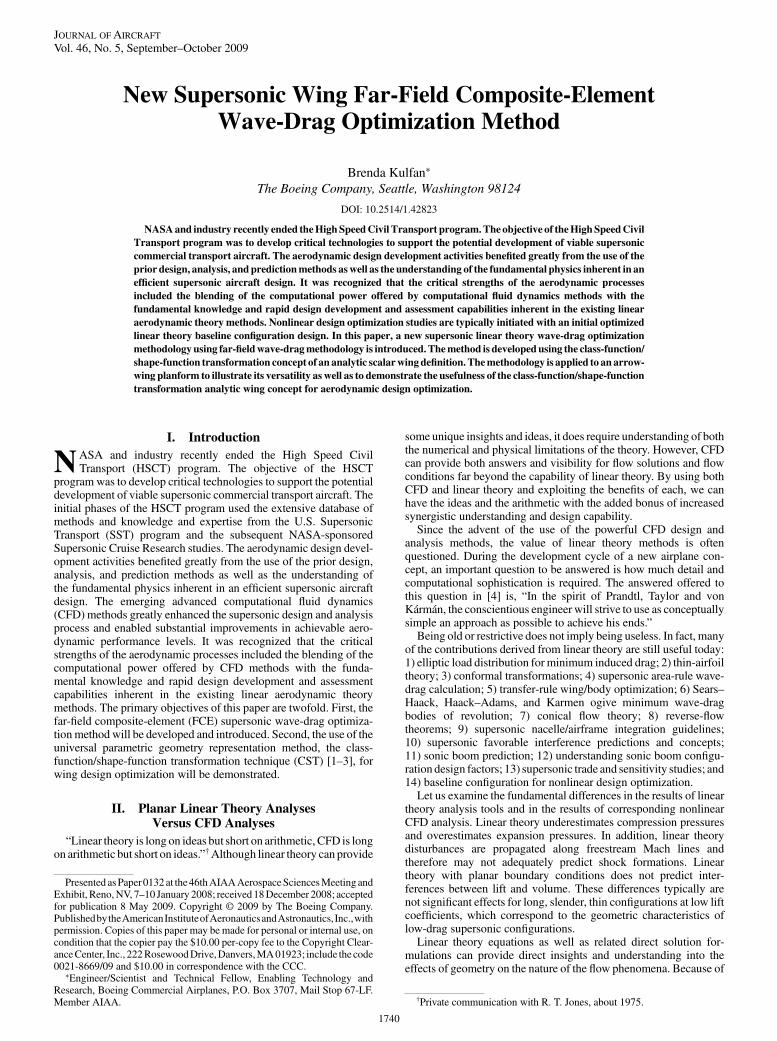
Early U.S. SST development studies, such as those shown inFig. 1, have confirmed that linear theory aerodynamic designsthat satisfy the set of pressure-coefficient-limiting real-flow designcriteria described in [5,6] achieve the theoretical inviscid draglevels and the friction drag in the wind tunnel. The figure on theleft is a comparison of the drag polar predicted by linear theory

with The Boeing Company test data for U.S. SST model 733-290.This was a linear-theory-optimized design of the configuration thatallowed Boeing to win the SST design development Governmentcontract. The friction drag CDF was computed by the T� method[7]. The volume wave drag CDW was calculated by a Boeing-developed zero-lift wave-drag program that was the basis for theNASA wave-drag program [8]. The drag due to lift CDL wascalculated using the Boeing/NASA system of supersonic andanalysis programs [9]. The linear theory prediction agrees verywell with the test data.

The figure on the right is a comparison of the linear theorypredictionswith test data for theU.S. SSTmodel 733-390. Thiswas alinear design of the last variable-sweep configuration that Boeingstudied before the final switch to the U.S. SST double-deltaconfiguration, B2707-300. The same drag prediction methods wereused as for the 733-290 configuration. Again, the linear theoryprediction agrees very well with the test data. The designs developedby linear theory designs were heavily constrained by the real-flowconstraints [5,6] and are therefore considered to be on the conser-vative side in terms of the aerodynamic performance. Hence, it is notsurprising that the inviscid predictions of dragmatch thewind-tunneltest data.

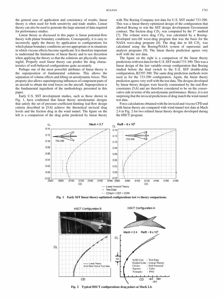
Force calculations obtainedwith the inviscid and viscousCFD andwith linear theory are compared with wind-tunnel test data at Mach2.4 in Fig. 2 for two refined linear theory designs developed duringthe HSCT program.

Fig. 1 Early SST linear-theory-optimized configurations test vs theory comparisons.

Fig. 2 Typical HSCT configurations drag polars at Mach 2.4.

KULFAN 1741

The inviscid codes included linear theory, the TRANAIR fullpotential code, and a parabolized Euler code. The viscous analyseswere obtained with a parabolized Navier–Stokes (PNS) code. Flat-plate skin-friction drag estimates were added to the inviscid CFDdrag calculations and to the linear theory and Euler predictions toobtain the total aerodynamic drag. The viscous and inviscid lift anddrag predictions all agree quite well with the test data. The lineartheory drag predictions depart from the test data at the higher liftcoefficient above the design condition.

These various test versus theory comparisons illustrate that lineartheory as used in this paper can provide accurate assessments ofthe aerodynamic forces near the 1 g cruise conditions that typicallycorrespond to the design optimization conditions. These results,together with extensive experience on the HSCT program, indicatethat a good initial linear-theory-optimized design can provide thebasis for developing nonlinear CFD-optimized designs.

III. Supersonic-Drag Components

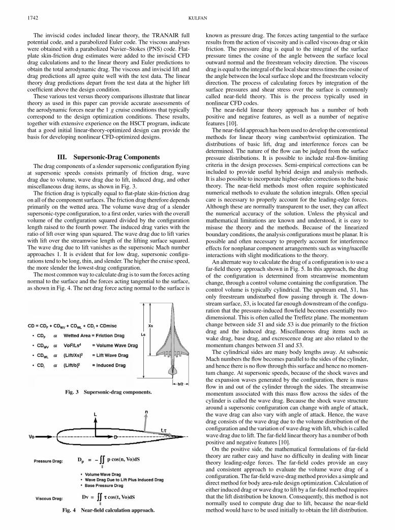
The drag components of a slender supersonic configuration flyingat supersonic speeds consists primarily of friction drag, wavedrag due to volume, wave drag due to lift, induced drag, and othermiscellaneous drag items, as shown in Fig. 3.

The friction drag is typically equal to flat-plate skin-friction dragon all of the component surfaces. The friction drag therefore dependsprimarily on the wetted area. The volume wave drag of a slendersupersonic-type configuration, to a first order, varies with the overallvolume of the configuration squared divided by the configurationlength raised to the fourth power. The induced drag varies with theratio of lift over wing span squared. The wave drag due to lift varieswith lift over the streamwise length of the lifting surface squared.The wave drag due to lift vanishes as the supersonic Mach numberapproaches 1. It is evident that for low drag, supersonic configu-rations tend to be long, thin, and slender. The higher the cruise speed,the more slender the lowest-drag configuration.

Themost commonway to calculate drag is to sum the forces actingnormal to the surface and the forces acting tangential to the surface,as shown in Fig. 4. The net drag force acting normal to the surface is

known as pressure drag. The forces acting tangential to the surfaceresults from the action of viscosity and is called viscous drag or skinfriction. The pressure drag is equal to the integral of the surfacepressure times the cosine of the angle between the surface localoutward normal and the freestream velocity direction. The viscousdrag is equal to the integral of the local shear stress times the cosine ofthe angle between the local surface slope and the freestream velocitydirection. The process of calculating forces by integration of thesurface pressures and shear stress over the surface is commonlycalled near-field theory. This is the process typically used innonlinear CFD codes.

The near-field linear theory approach has a number of bothpositive and negative features, as well as a number of negativefeatures [10].

The near-field approach has been used to develop the conventionalmethods for linear theory wing camber/twist optimization. Thedistributions of basic lift, drag and interference forces can bedetermined. The nature of the flow can be judged from the surfacepressure distributions. It is possible to include real-flow-limitingcriteria in the design processes. Semi-empirical corrections can beincluded to provide useful hybrid design and analysis methods.It is also possible to incorporate higher-order corrections to the basictheory. The near-field methods most often require sophisticatednumerical methods to evaluate the solution integrals. Often specialcare is necessary to properly account for the leading-edge forces.Although these are normally transparent to the user, they can affectthe numerical accuracy of the solution. Unless the physical andmathematical limitations are known and understood, it is easy tomisuse the theory and the methods. Because of the linearizedboundary conditions, the analysis configurations must be planar. It ispossible and often necessary to properly account for interferenceeffects for nonplanar component arrangements such as wing/nacelleinteractions with slight modifications to the theory.

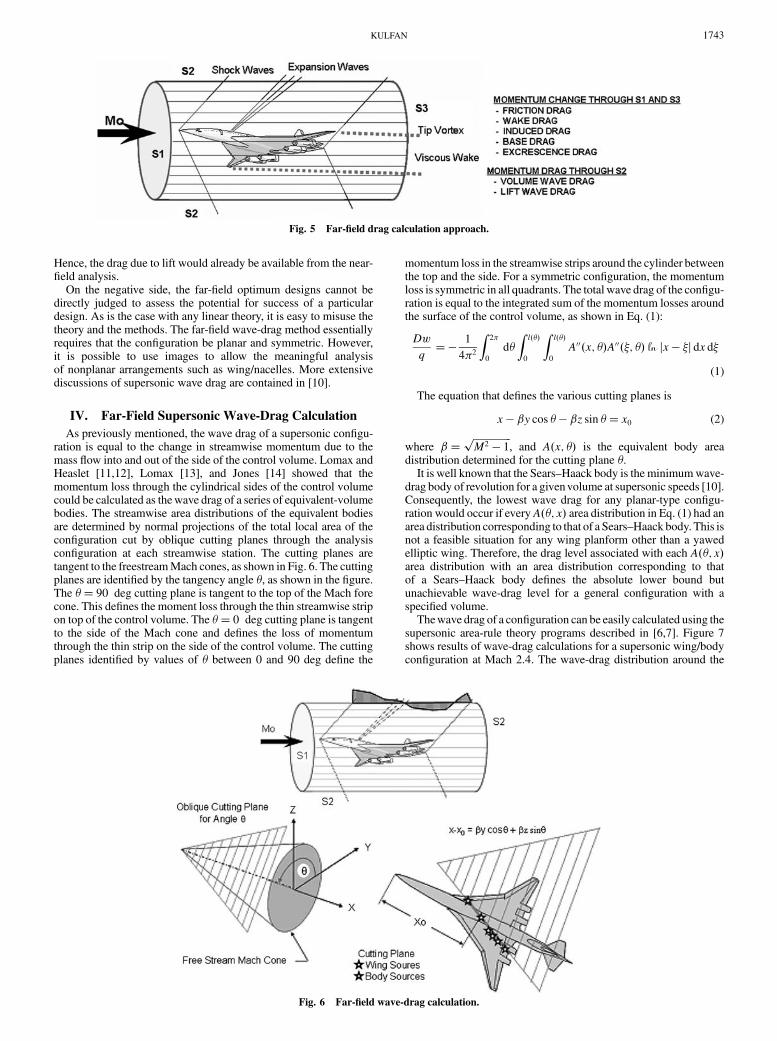
An alternate way to calculate the drag of a configuration is to use afar-field theory approach shown in Fig. 5. In this approach, the dragof the configuration is determined from streamwise momentumchange, through a control volume containing the configuration. Thecontrol volume is typically cylindrical. The upstream end, S1, hasonly freestream undisturbed flow passing through it. The down-stream surface, S3, is located far enough downstream of the configu-ration that the pressure-induced flowfield becomes essentially two-dimensional. This is often called the Treffetz plane. The momentumchange between side S1 and side S3 is due primarily to the frictiondrag and the induced drag. Miscellaneous drag items such aswake drag, base drag, and excrescence drag are also related to themomentum changes between S1 and S3.

The cylindrical sides are many body lengths away. At subsonicMach numbers the flow becomes parallel to the sides of the cylinder,and hence there is no flow through this surface and hence nomomen-tum change. At supersonic speeds, because of the shock waves andthe expansion waves generated by the configuration, there is massflow in and out of the cylinder through the sides. The streamwisemomentum associated with this mass flow across the sides of thecylinder is called the wave drag. Because the shock wave structurearound a supersonic configuration can change with angle of attack,the wave drag can also vary with angle of attack. Hence, the wavedrag consists of the wave drag due to the volume distribution of theconfiguration and the variation of wave drag with lift, which is calledwave drag due to lift. The far-field linear theory has a number of bothpositive and negative features [10].

On the positive side, the mathematical formulations of far-fieldtheory are rather easy and have no difficulty in dealing with lineartheory leading-edge forces. The far-field codes provide an easyand consistent approach to evaluate the volume wave drag of aconfiguration. The far-field wave-dragmethod provides a simple anddirect method for body area-rule design optimization. Calculation ofeither induced drag or wave drag to lift by a far-field method requiresthat the lift distribution be known. Consequently, this method is notnormally used to compute drag due to lift, because the near-fieldmethod would have to be used initially to obtain the lift distribution.

Fig. 3 Supersonic-drag components.

Fig. 4 Near-field calculation approach.

1742 KULFAN

Hence, the drag due to lift would already be available from the near-field analysis.

On the negative side, the far-field optimum designs cannot bedirectly judged to assess the potential for success of a particulardesign. As is the case with any linear theory, it is easy to misuse thetheory and the methods. The far-field wave-drag method essentiallyrequires that the configuration be planar and symmetric. However,it is possible to use images to allow the meaningful analysisof nonplanar arrangements such as wing/nacelles. More extensivediscussions of supersonic wave drag are contained in [10].

IV. Far-Field Supersonic Wave-Drag Calculation

As previously mentioned, the wave drag of a supersonic configu-ration is equal to the change in streamwise momentum due to themass flow into and out of the side of the control volume. Lomax andHeaslet [11,12], Lomax [13], and Jones [14] showed that themomentum loss through the cylindrical sides of the control volumecould be calculated as thewave drag of a series of equivalent-volumebodies. The streamwise area distributions of the equivalent bodiesare determined by normal projections of the total local area of theconfiguration cut by oblique cutting planes through the analysisconfiguration at each streamwise station. The cutting planes aretangent to the freestreamMach cones, as shown in Fig. 6. The cuttingplanes are identified by the tangency angle �, as shown in the figure.The �� 90 deg cutting plane is tangent to the top of the Mach forecone. This defines the moment loss through the thin streamwise stripon top of the control volume. The �� 0 deg cutting plane is tangentto the side of the Mach cone and defines the loss of momentumthrough the thin strip on the side of the control volume. The cuttingplanes identified by values of � between 0 and 90 deg define the

momentum loss in the streamwise strips around the cylinder betweenthe top and the side. For a symmetric configuration, the momentumloss is symmetric in all quadrants. The total wave drag of the configu-ration is equal to the integrated sum of the momentum losses aroundthe surface of the control volume, as shown in Eq. (1):

Dw

q�� 1

4�2

Z2�

0

d�

Zl���

0

Zl���

0

A00�x; ��A00��; �� ln jx � �j dx d�

(1)

The equation that defines the various cutting planes is

x � �y cos � � �z sin �� x0 (2)

where ������������������M2 � 1p

, and A�x; �� is the equivalent body areadistribution determined for the cutting plane �.

It is well known that the Sears–Haack body is the minimumwave-drag body of revolution for a givenvolume at supersonic speeds [10].Consequently, the lowest wave drag for any planar-type configu-ration would occur if everyA��; x� area distribution in Eq. (1) had anarea distribution corresponding to that of a Sears–Haack body. This isnot a feasible situation for any wing planform other than a yawedelliptic wing. Therefore, the drag level associated with each A��; x�area distribution with an area distribution corresponding to thatof a Sears–Haack body defines the absolute lower bound butunachievable wave-drag level for a general configuration with aspecified volume.

Thewave drag of a configuration can be easily calculated using thesupersonic area-rule theory programs described in [6,7]. Figure 7shows results of wave-drag calculations for a supersonic wing/bodyconfiguration at Mach 2.4. The wave-drag distribution around the

Fig. 5 Far-field drag calculation approach.

Fig. 6 Far-field wave-drag calculation.

KULFAN 1743

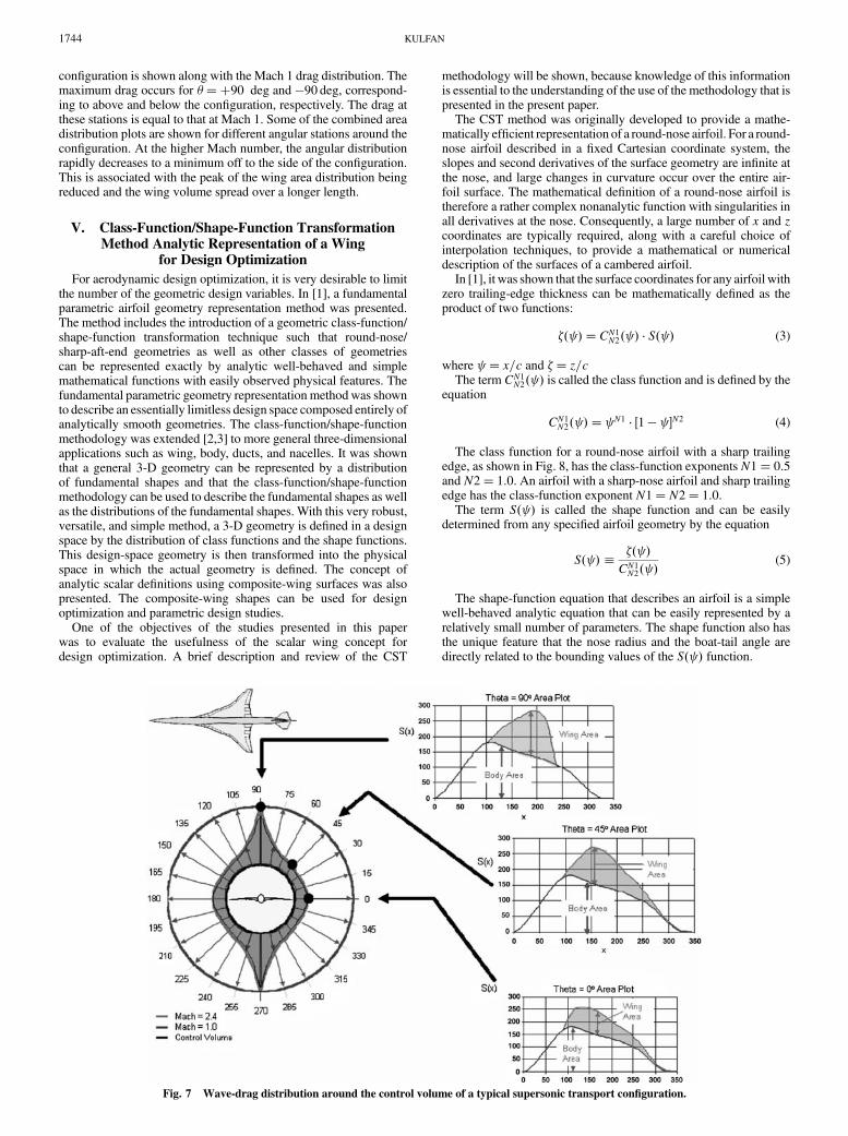
configuration is shown along with the Mach 1 drag distribution. Themaximum drag occurs for ���90 deg and �90 deg, correspond-ing to above and below the configuration, respectively. The drag atthese stations is equal to that at Mach 1. Some of the combined areadistribution plots are shown for different angular stations around theconfiguration. At the higher Mach number, the angular distributionrapidly decreases to a minimum off to the side of the configuration.This is associated with the peak of the wing area distribution beingreduced and the wing volume spread over a longer length.

V. Class-Function/Shape-Function TransformationMethod Analytic Representation of a Wing

for Design Optimization

For aerodynamic design optimization, it is very desirable to limitthe number of the geometric design variables. In [1], a fundamentalparametric airfoil geometry representation method was presented.The method includes the introduction of a geometric class-function/shape-function transformation technique such that round-nose/sharp-aft-end geometries as well as other classes of geometriescan be represented exactly by analytic well-behaved and simplemathematical functions with easily observed physical features. Thefundamental parametric geometry representationmethodwas shownto describe an essentially limitless design space composed entirely ofanalytically smooth geometries. The class-function/shape-functionmethodology was extended [2,3] to more general three-dimensionalapplications such as wing, body, ducts, and nacelles. It was shownthat a general 3-D geometry can be represented by a distributionof fundamental shapes and that the class-function/shape-functionmethodology can be used to describe the fundamental shapes as wellas the distributions of the fundamental shapes. With this very robust,versatile, and simple method, a 3-D geometry is defined in a designspace by the distribution of class functions and the shape functions.This design-space geometry is then transformed into the physicalspace in which the actual geometry is defined. The concept ofanalytic scalar definitions using composite-wing surfaces was alsopresented. The composite-wing shapes can be used for designoptimization and parametric design studies.

One of the objectives of the studies presented in this paperwas to evaluate the usefulness of the scalar wing concept fordesign optimization. A brief description and review of the CST

methodology will be shown, because knowledge of this informationis essential to the understanding of the use of the methodology that ispresented in the present paper.

The CST method was originally developed to provide a mathe-matically efficient representation of a round-nose airfoil. For a round-nose airfoil described in a fixed Cartesian coordinate system, theslopes and second derivatives of the surface geometry are infinite atthe nose, and large changes in curvature occur over the entire air-foil surface. The mathematical definition of a round-nose airfoil istherefore a rather complex nonanalytic function with singularities inall derivatives at the nose. Consequently, a large number of x and zcoordinates are typically required, along with a careful choice ofinterpolation techniques, to provide a mathematical or numericaldescription of the surfaces of a cambered airfoil.

In [1], it was shown that the surface coordinates for any airfoil withzero trailing-edge thickness can be mathematically defined as theproduct of two functions:

�� � � CN1N2� � � S� � (3)

where � x=c and �� z=cThe term CN1N2� � is called the class function and is defined by the

equation

CN1N2� � � N1 � �1 � N2 (4)

The class function for a round-nose airfoil with a sharp trailingedge, as shown in Fig. 8, has the class-function exponentsN1� 0:5and N2� 1:0. An airfoil with a sharp-nose airfoil and sharp trailingedge has the class-function exponent N1� N2� 1:0.

The term S� � is called the shape function and can be easilydetermined from any specified airfoil geometry by the equation

S� � �� �CN1N2� �

(5)

The shape-function equation that describes an airfoil is a simplewell-behaved analytic equation that can be easily represented by arelatively small number of parameters. The shape function also hasthe unique feature that the nose radius and the boat-tail angle aredirectly related to the bounding values of the S� � function.

Fig. 7 Wave-drag distribution around the control volume of a typical supersonic transport configuration.

1744 KULFAN

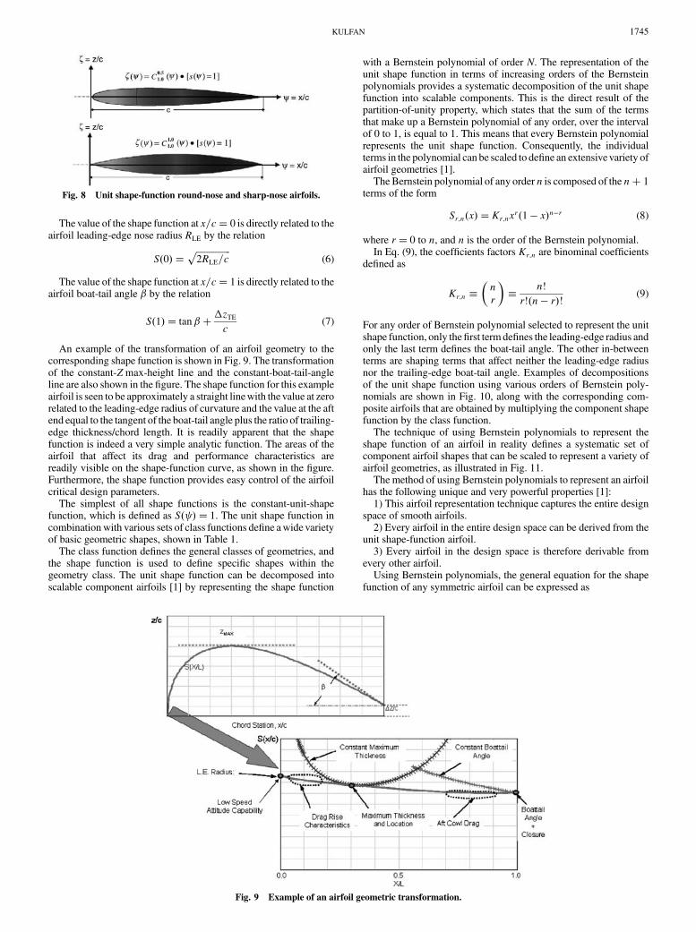
The value of the shape function at x=c� 0 is directly related to theairfoil leading-edge nose radius RLE by the relation

S�0� �����������������2RLE=c

p(6)

The value of the shape function at x=c� 1 is directly related to theairfoil boat-tail angle � by the relation

S�1� � tan���zTEc

(7)

An example of the transformation of an airfoil geometry to thecorresponding shape function is shown in Fig. 9. The transformationof the constant-Zmax-height line and the constant-boat-tail-angleline are also shown in the figure. The shape function for this exampleairfoil is seen to be approximately a straight linewith the value at zerorelated to the leading-edge radius of curvature and the value at the aftend equal to the tangent of the boat-tail angle plus the ratio of trailing-edge thickness/chord length. It is readily apparent that the shapefunction is indeed a very simple analytic function. The areas of theairfoil that affect its drag and performance characteristics arereadily visible on the shape-function curve, as shown in the figure.Furthermore, the shape function provides easy control of the airfoilcritical design parameters.

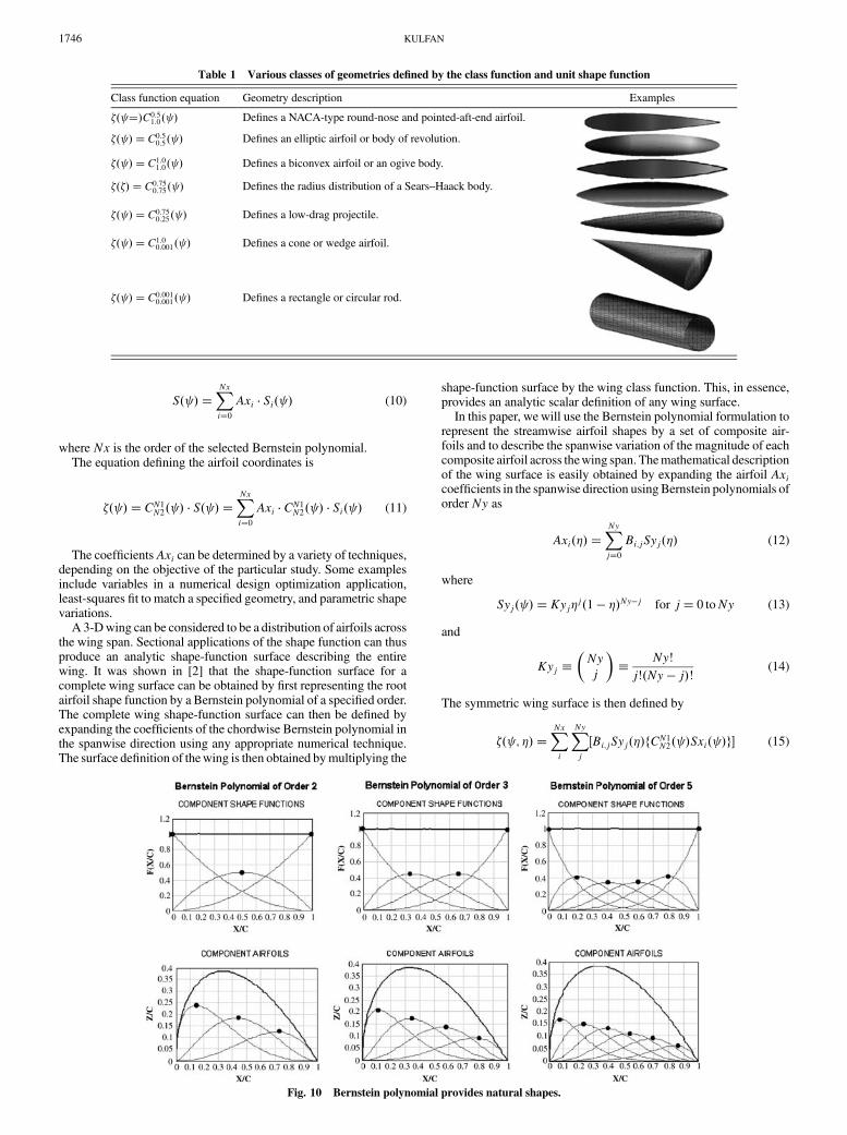
The simplest of all shape functions is the constant-unit-shapefunction, which is defined as S� � � 1. The unit shape function incombinationwith various sets of class functions define awide varietyof basic geometric shapes, shown in Table 1.

The class function defines the general classes of geometries, andthe shape function is used to define specific shapes within thegeometry class. The unit shape function can be decomposed intoscalable component airfoils [1] by representing the shape function

with a Bernstein polynomial of order N. The representation of theunit shape function in terms of increasing orders of the Bernsteinpolynomials provides a systematic decomposition of the unit shapefunction into scalable components. This is the direct result of thepartition-of-unity property, which states that the sum of the termsthat make up a Bernstein polynomial of any order, over the intervalof 0 to 1, is equal to 1. This means that every Bernstein polynomialrepresents the unit shape function. Consequently, the individualterms in the polynomial can be scaled to define an extensivevariety ofairfoil geometries [1].

The Bernstein polynomial of any order n is composed of the n� 1terms of the form

Sr;n�x� � Kr;nxr�1 � x�n�r (8)

where r� 0 to n, and n is the order of the Bernstein polynomial.In Eq. (9), the coefficients factors Kr;n are binominal coefficients

defined as

Kr;n nr

� � n!

r!�n � r�! (9)

For any order of Bernstein polynomial selected to represent the unitshape function, only thefirst term defines the leading-edge radius andonly the last term defines the boat-tail angle. The other in-betweenterms are shaping terms that affect neither the leading-edge radiusnor the trailing-edge boat-tail angle. Examples of decompositionsof the unit shape function using various orders of Bernstein poly-nomials are shown in Fig. 10, along with the corresponding com-posite airfoils that are obtained by multiplying the component shapefunction by the class function.

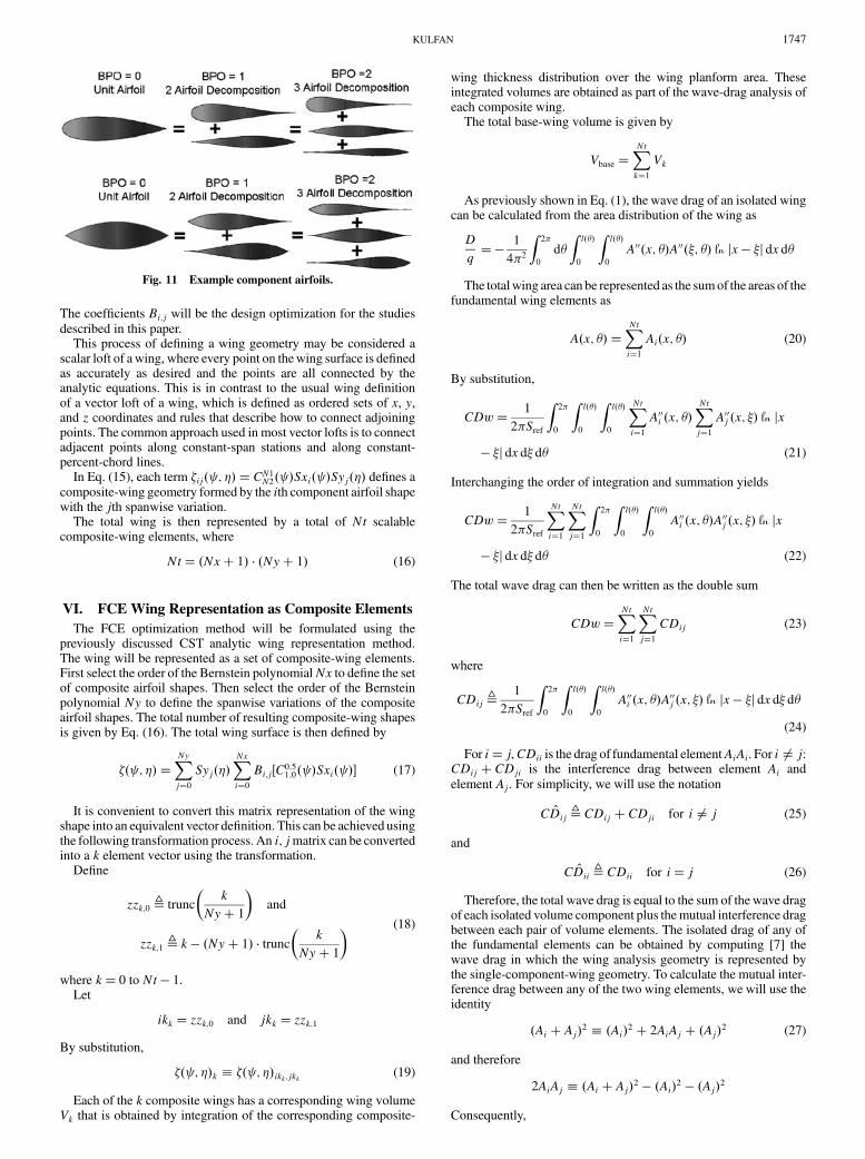
The technique of using Bernstein polynomials to represent theshape function of an airfoil in reality defines a systematic set ofcomponent airfoil shapes that can be scaled to represent a variety ofairfoil geometries, as illustrated in Fig. 11.

The method of using Bernstein polynomials to represent an airfoilhas the following unique and very powerful properties [1]:

1) This airfoil representation technique captures the entire designspace of smooth airfoils.

2) Every airfoil in the entire design space can be derived from theunit shape-function airfoil.

3) Every airfoil in the design space is therefore derivable fromevery other airfoil.

Using Bernstein polynomials, the general equation for the shapefunction of any symmetric airfoil can be expressed as

Fig. 8 Unit shape-function round-nose and sharp-nose airfoils.

Fig. 9 Example of an airfoil geometric transformation.

KULFAN 1745

S� � �XNxi�0

Axi � Si� � (10)

where Nx is the order of the selected Bernstein polynomial.The equation defining the airfoil coordinates is

�� � � CN1N2� � � S� � �XNxi�0

Axi � CN1N2� � � Si� � (11)

The coefficients Axi can be determined by a variety of techniques,depending on the objective of the particular study. Some examplesinclude variables in a numerical design optimization application,least-squares fit to match a specified geometry, and parametric shapevariations.

A 3-Dwing can be considered to be a distribution of airfoils acrossthe wing span. Sectional applications of the shape function can thusproduce an analytic shape-function surface describing the entirewing. It was shown in [2] that the shape-function surface for acomplete wing surface can be obtained by first representing the rootairfoil shape function by a Bernstein polynomial of a specified order.The complete wing shape-function surface can then be defined byexpanding the coefficients of the chordwise Bernstein polynomial inthe spanwise direction using any appropriate numerical technique.The surface definition of thewing is then obtained bymultiplying the

shape-function surface by the wing class function. This, in essence,provides an analytic scalar definition of any wing surface.

In this paper, we will use the Bernstein polynomial formulation torepresent the streamwise airfoil shapes by a set of composite air-foils and to describe the spanwise variation of the magnitude of eachcomposite airfoil across thewing span. Themathematical descriptionof the wing surface is easily obtained by expanding the airfoil Axicoefficients in the spanwise direction usingBernstein polynomials oforder Ny as

Axi��� �XNyj�0

Bi;jSyj��� (12)

where

Syj� � � Kyj�j�1 � ��Ny�j for j� 0 toNy (13)

and

Kyj Nyj

� � Ny!

j!�Ny � j�! (14)

The symmetric wing surface is then defined by

�� ; �� �XNxi

XNyj

�Bi;jSyj���fCN1N2� �Sxi� �g (15)

Table 1 Various classes of geometries defined by the class function and unit shape function

Class function equation Geometry description Examples

�� ��C0:51:0� � Defines a NACA-type round-nose and pointed-aft-end airfoil.

�� � � C0:50:5� � Defines an elliptic airfoil or body of revolution.

�� � � C1:01:0� � Defines a biconvex airfoil or an ogive body.

���� � C0:750:75� � Defines the radius distribution of a Sears–Haack body.

�� � � C0:750:25� � Defines a low-drag projectile.

�� � � C1:00:001� � Defines a cone or wedge airfoil.

�� � � C0:0010:001� � Defines a rectangle or circular rod.

Fig. 10 Bernstein polynomial provides natural shapes.

1746 KULFAN

The coefficients Bi;j will be the design optimization for the studiesdescribed in this paper.

This process of defining a wing geometry may be considered ascalar loft of a wing, where every point on thewing surface is definedas accurately as desired and the points are all connected by theanalytic equations. This is in contrast to the usual wing definitionof a vector loft of a wing, which is defined as ordered sets of x, y,and z coordinates and rules that describe how to connect adjoiningpoints. The common approach used in most vector lofts is to connectadjacent points along constant-span stations and along constant-percent-chord lines.

In Eq. (15), each term �ij� ; �� � CN1N2� �Sxi� �Syj��� defines acomposite-wing geometry formed by the ith component airfoil shapewith the jth spanwise variation.

The total wing is then represented by a total of Nt scalablecomposite-wing elements, where

Nt� �Nx� 1� � �Ny� 1� (16)

VI. FCE Wing Representation as Composite Elements

The FCE optimization method will be formulated using thepreviously discussed CST analytic wing representation method.The wing will be represented as a set of composite-wing elements.First select the order of the Bernstein polynomialNx to define the setof composite airfoil shapes. Then select the order of the Bernsteinpolynomial Ny to define the spanwise variations of the compositeairfoil shapes. The total number of resulting composite-wing shapesis given by Eq. (16). The total wing surface is then defined by

�� ; �� �XNyj�0

Syj���XNxi�0

Bi;j�C0:51:0� �Sxi� � (17)

It is convenient to convert this matrix representation of the wingshape into an equivalent vector definition. This can be achieved usingthe following transformation process. An i; jmatrix can be convertedinto a k element vector using the transformation.

Define

zzk;0 ≜ trunc

�k

Ny� 1

�and

zzk;1 ≜ k � �Ny� 1� � trunc�

k

Ny� 1

� (18)

where k� 0 to Nt � 1.Let

ikk � zzk;0 and jkk � zzk;1

By substitution,

�� ; ��k �� ; ��ikk;jkk (19)

Each of the k composite wings has a corresponding wing volumeVk that is obtained by integration of the corresponding composite-

wing thickness distribution over the wing planform area. Theseintegrated volumes are obtained as part of the wave-drag analysis ofeach composite wing.

The total base-wing volume is given by

Vbase �XNtk�1

Vk

As previously shown in Eq. (1), the wave drag of an isolated wingcan be calculated from the area distribution of the wing as

D

q�� 1

4�2

Z2�

0

d�

Zl���

0

Zl���

0

A00�x; ��A00��; �� ln jx � �j dx d�

The totalwing area can be represented as the sumof the areas of thefundamental wing elements as

A�x; �� �XNti�1

Ai�x; �� (20)

By substitution,

CDw� 1

2�Sref

Z2�

0

Zl���

0

Zl���

0

XNti�1

A00i �x; ��XNtj�1

A00j �x; �� ln jx

� �j dx d� d� (21)

Interchanging the order of integration and summation yields

CDw� 1

2�Sref

XNti�1

XNtj�1

Z2�

0

Zl���

0

Zl���

0

A00i �x; ��A00j �x; �� ln jx

� �j dx d� d� (22)

The total wave drag can then be written as the double sum

CDw�XNti�1

XNtj�1

CDij (23)

where

CDij ≜1

2�Sref

Z2�

0

Zl���

0

Zl���

0

A00i �x; ��A00j �x; �� ln jx � �j dx d� d�

(24)

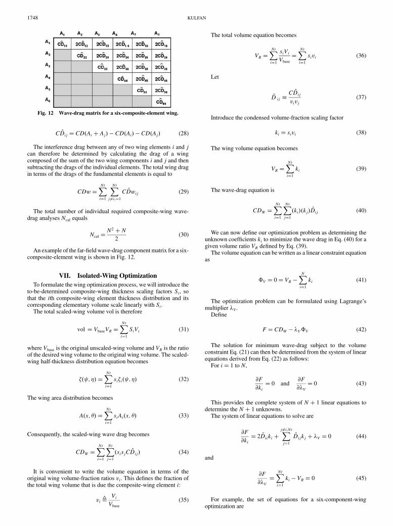
For i� j,CDii is the drag of fundamental elementAiAi. For i ≠ j:CDij � CDji is the interference drag between element Ai andelement Aj. For simplicity, we will use the notation

CD̂ij ≜ CDij � CDji for i ≠ j (25)

and

CD̂ii ≜ CDii for i� j (26)

Therefore, the total wave drag is equal to the sum of the wave dragof each isolated volume component plus themutual interference dragbetween each pair of volume elements. The isolated drag of any ofthe fundamental elements can be obtained by computing [7] thewave drag in which the wing analysis geometry is represented bythe single-component-wing geometry. To calculate the mutual inter-ference drag between any of the two wing elements, we will use theidentity

�Ai � Aj�2 �Ai�2 � 2AiAj � �Aj�2 (27)

and therefore

2AiAj �Ai � Aj�2 � �Ai�2 � �Aj�2

Consequently,

Fig. 11 Example component airfoils.

KULFAN 1747

CD̂ij � CD�Ai � Aj� � CD�Ai� � CD�Aj� (28)

The interference drag between any of two wing elements i and jcan therefore be determined by calculating the drag of a wingcomposed of the sum of the two wing components i and j and thensubtracting the drags of the individual elements. The total wing dragin terms of the drags of the fundamental elements is equal to

CDw�XNti�1

XNtj≠i;�1

CD̂wij (29)

The total number of individual required composite-wing wave-drag analyses Ncal equals

Ncal �N2 � N

2(30)

An example of the far-field wave-drag component matrix for a six-composite-element wing is shown in Fig. 12.

VII. Isolated-Wing Optimization

To formulate the wing optimization process, we will introduce theto-be-determined composite-wing thickness scaling factors Si, sothat the ith composite-wing element thickness distribution and itscorresponding elementary volume scale linearly with Si.

The total scaled-wing volume vol is therefore

vol � VbaseVR �XNti�1

SiVi (31)

where Vbase is the original unscaled-wing volume and VR is the ratioof the desired wing volume to the original wing volume. The scaled-wing half-thickness distribution equation becomes

�� ; �� �XNti�1

si�i� ; �� (32)

The wing area distribution becomes

A�x; �� �XNti�1

siAi�x; �� (33)

Consequently, the scaled-wing wave drag becomes

CDW �XNti�1

XNtj�1�sisjCD̂ij� (34)

It is convenient to write the volume equation in terms of theoriginal wing volume-fraction ratios vi. This defines the fraction ofthe total wing volume that is due the composite-wing element i:

vi ≜ViVbase

(35)

The total volume equation becomes

VR �XNti�1

siViVbase

�XNti�1

sivi (36)

Let

~D ij CD̂ij

vivj(37)

Introduce the condensed volume-fraction scaling factor

ki � sivi (38)

The wing volume equation becomes

VR �XNti�1

ki (39)

The wave-drag equation is

CDW �XNti�1

XNtj�1�ki��kj� ~Dij (40)

We can now define our optimization problem as determining theunknown coefficients ki to minimize the wave drag in Eq. (40) for agiven volume ratio VR defined by Eq. (39).

The volume equation can bewritten as a linear constraint equationas

�V � 0� VR �XNi�1

ki (41)

The optimization problem can be formulated using Lagrange’smultiplier �V.

Define

F� CDW � �V�V (42)

The solution for minimum wave-drag subject to the volumeconstraint Eq. (21) can then be determined from the system of linearequations derived from Eq. (22) as follows:

For i� 1 to N,

@F

@ki� 0 and

@F

@�V� 0 (43)

This provides the complete system of N � 1 linear equations todetermine the N � 1 unknowns.

The system of linear equations to solve are

@F

@ki� 2 ~Diiki �

Xj≠i;Ntj�1

D̂ijkj � �V � 0 (44)

and

@F

@�V�XNti�1

ki � VR � 0 (45)

For example, the set of equations for a six-component-wingoptimization are

Fig. 12 Wave-drag matrix for a six-composite-element wing.

1748 KULFAN

2 ~D11k1 � ~D12k2 � ~D13k3 � ~D14k4 � ~D15k5 � ~D16k6 � �V � 0

~D21k1 � 2 ~D22k2 � ~D23k3 � ~D24k4 � ~D25k5 � ~D26k6 � �V � 0

~D31k1 � ~D32k2 � 2 ~D33k3 � ~D34k4 � ~D35k5 � ~D36k6 � �V � 0

~D41k1 � ~D42k2 � ~D43k3 � 2 ~D44k4 � ~D45k5 � ~D46k6 � �V � 0

~D51k1 � ~D52k2 � ~D53k3 � ~D54k4 � 2 ~D55k5 � ~D56k6 � �V � 0

~D61k1 � ~D62k2 � ~D63k3 � ~D64k4 � ~D65k5 � 2 ~D66k6 � �V � 0

k1 � k2 � k3 � k4 � k5 � k6 � 0� VR

The solution to these equations can be expressed in matrix form as

2 ~D11~D12

~D13 � � � ~D1N 1~D21 2 ~D22

~D23 � � � ~D2N 1~D31

~D32 2 ~D33 � � � ~D3N 1

..

. ... ..

. . .. ..

. ...

~DN1~DN2

~DN3 � � � 2 ~DNN 1

1 1 1 1 1 0

266666664

377777775

k1k2k3...

kN�V

266666664

377777775�

0

0

0

..

.

0

VR

26666664

37777775

The matrix equations can be written in condensed form as

�D�k � �R (46)

The solution for the unknowns ki and �V is easily obtained bymatrix inversion as

�D�R�1 � �k (47)

The solution to the equations is given by the values of ki. Theoptimized composite-wing scaling factors are calculated from ki as

si � kiVbase

Vi(48)

The optimum z=c distribution is calculated from Eq. (32) and thecorresponding minimum wave drag is obtained from Eq. (34).

VIII. Including Fuselage and NacelleInterference Effects

The drag of a wing/body configuration can be calculated usingEq. (1) with the wing/body combined area distribution. The areadistributions consist of the wing area AW plus the body area ABdistributions:

At�x; �� � AW�x; �� � AB�x� (49)

Substituting Eq. (49) into Eq. (1) indicates that thewing/body dragconsists of three components:

The drag of the isolated wing is

CDwwing �1

2�Sref

Z2�

0

Zl���

0

Zl���

0

A00W�x; ��A00W��; �� ln jx

� �j dx d� d� (50)

The drag of the isolated body is

CDwbody �1

Sref

ZLB

0

ZLB

0

A00B�x�A00B��� ln jx � �j dx d� (51)

Wing/body interference drag is

CDwWBint �2

2�Sref

Z2�

0

Zl���

0

Zl���

0

A00B���A00W�x; �� ln jx

� �j dx d� d� (52)

The wing area distribution can be represented as the sum of theareas of the fundamental wing elements:

Aw�x; �� �XNti�1

Ai�x; �� (53)

The wing/body interference drag then becomes

CDwWBint �2

2�Sref

Z2�

0

Zl���

0

Zl���

0

A00B���XNti�1

A00i �x; �� ln jx

� �j dx d� d� (54)

Interchanging the order of summation and integration gives

CDwWBint �1

�Sref

XNti�1

Z2�

0

Zl���

0

Zl���

0

A00B���A00i �x; �� ln jx

� �j dx d� d� (55)

Define the interference drag between the body and wing elementAi, CDwbi, as

CDwbi ≜1

�Sref

Z2�

0

Zl���

0

Zl���

0

A00B���A00i ��� ln jx � �j dx d� d�

(56)

Therefore,

CDwWBint �XNi�1

CDwbi (57)

The wing/body interference drag is equal to the sum of theinterference drags of the body with each of the isolated-wingelements. To calculate CDwbi, use the identity

�AB � Ai2 A2B � 2ABAi � A2

i (58)

Consequently,

CDwbi � CD�AB � Ai� � CD�Ai� � CD�AB� (59)

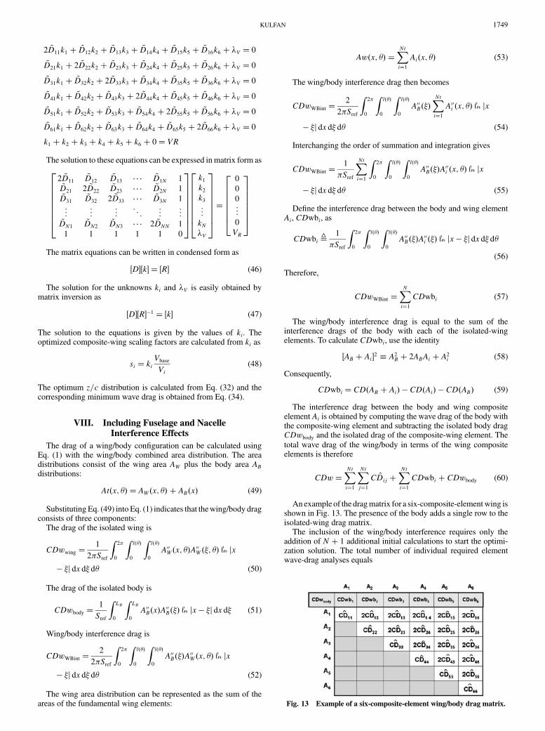
The interference drag between the body and wing compositeelement Ai is obtained by computing the wave drag of the body withthe composite-wing element and subtracting the isolated body dragCDwbody and the isolated drag of the composite-wing element. Thetotal wave drag of the wing/body in terms of the wing compositeelements is therefore

CDw�XNti�1

XNtj�1

CD̂ij �XNti�1

CDwbi � CDwbody (60)

An example of the dragmatrix for a six-composite-elementwing isshown in Fig. 13. The presence of the body adds a single row to theisolated-wing drag matrix.

The inclusion of the wing/body interference requires only theaddition of N � 1 additional initial calculations to start the optimi-zation solution. The total number of individual required elementwave-drag analyses equals

Fig. 13 Example of a six-composite-element wing/body drag matrix.

KULFAN 1749

Ncal �N2 � N

2� N � 1 (61)

The wing/body drag equation in terms of arbitrary scalingcoefficients si is

CDW � CDbody �XNti�1

XNtj�1�si�i��sj�j�

CDij

i�j�XNti�1�si�i�

CDwbi�i

(62)

As previously noted,

D̂ ij ≜CD̂ij

vivjand ki ≜ sivi

Let

Dwbi ≜CDwbivi

(63)

The total wave-drag equation in terms of the to-be-determinedoptimization variables ki becomes

CDW � CDbody �XNti�1

XNtj�1�ki��kj�Dij �

XNti�1�ki�Dwbi (64)

We will follow the same optimization procedure with Lagrange’smultipliers as for the isolated-wing case. The system of linearequations to solve to determine the optimum wing geometry in thepresence of a body are

@F

@ki� 2Diiki �

Xj≠i;Ntj�1

Dijkj � �Dwbi � �V� � 0 (65)

together with the volume constraint equation:

@F

@�V� k1 � k2 � k3 � k4 � � � � kN � VR � 0 (66)

The solution equations for an example of six-composite-wingelements plus the body are

2 ~D11k1 � ~D12k2 � ~D13k3 � ~D14k4 � ~D15k5 � ~D16k6 � �V��Dwb1

~D21k1 � 2 ~D22k2 � ~D23k3 � ~D24k4 � ~D25k5 � ~D26k6 � �V��Dwb2

~D31k1 � ~D32k2 � 2 ~D33k3 � ~D34k4 � ~D35k5 � ~D36k6 � �V��Dwb3

~D41k1 � ~D42k2 � ~D43k3 � 2 ~D44k4 � ~D45k5 � ~D46k6 � �V��Dwb4

~D51k1 � ~D52k2 � ~D53k3 � ~D54k4 � 2 ~D55k5 � ~D56k6 � �V��Dwb5

~D61k1 � ~D62k2 � ~D63k3 � ~D64k4 � ~D65k5 � 2 ~D66k6 � �V��Dwb6

k1 � k2 � k3 � k4 � k5 � k6 � 0� VR

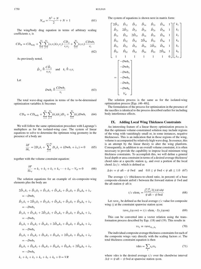
The system of equations is shown next in matrix form:

2 ~D11~D12

~D13~D14

~D15~D16 1

~D21 2 ~D22~D23

~D24~D25

~D26 1

~D31~D32 2 ~D33

~D34~D35

~D36 1

~D41~D42

~D43 2 ~D44~D45

~D46 1

~D51~D52

~D53~D54 2 ~D55

~D56 1

~D61~D62

~D63~D64

~D65 2 ~D66 1

1 1 1 1 1 1 0

266666666666664

377777777777775

k1

k2

k3

k4

k5

k6

�V

266666666666664

377777777777775

�

�Dwb1�Dwb2�Dwb3�Dwb4�Dwb5�Dwb6VR

266666666666664

377777777777775

The solution process is the same as for the isolated-wingoptimization process [Eqs. (46–48)].

The formulation of the process for optimization in the presence ofthe nacelles is identical to the process described earlier for includingbody interference effects.

IX. Adding Local Wing Thickness Constraints

An interesting feature of a linear theory optimization process isthat the optimum volume-constrained solution may include regionsof the wing with vanishingly small or, in some instances, negativethicknesses. This is an indication that in those regions of the wing,volume is accompanied by relatively highwave drag. In essence, thisis an attempt by the linear theory to alter the wing planform.Consequently, in addition to an overall volume constraint, it is oftennecessary to provide the capability to impose local minimum wingthickness constraints. To accomplish this, we will define a generallocal depth or area constraint in terms of a desired average thickness/chord ratio at a specific station �C and over a portion of the localchord �x=c. which is defined as

� c� aft � fwd and 0:0 � fwd< aft � 1:0 (67)

The average t=c (thickness-to-chord ratio, in percent) of a basecomposite-element airfoil i between the forward station fwd andthe aft station aft is

t=c elemi �R aft fwd 2�i� � d aft � fwd

(68)

Let aveij be defined as the local average t=c value for compositewing ij at the constraint spanwise station �con:

aveij��con� � t=c elemi � Syj��con� (69)

This can be converted into a vector relation using the trans-formation process described by Eqs. (18) and (19). This results in

vk aveikk;jkk (70)

The individual composite average thickness constraints for each ofthe composite wings vary directly with the scaling factors si. Thetotal thickness constraint equation is then

des�Xk

sktvk (71)

where des is the desired average t=c over the chordwise interval� � aft � fwd at spanwise station �con.

1750 KULFAN

Normalize this equation by the volume ratio of each of thecomposite wings to obtain

des�Xk

�skvk�tvkvk

(72)

Define

cnk tvkvk

The average thickness constraint equation becomes

�T � des �XNt�1q�0

kqcnq � 0 (73)

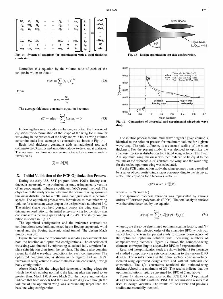
Following the same procedure as before, we obtain the linear set ofequations for determination of the shape of the wing for minimumwave drag in the presence of the body and with both a wing volumeconstraint and a local average t=c constraint, as shown in Fig. 14.

Each local thickness constraint adds an additional row andcolumn to theDmatrix and an additional row to the k andRmatrices.The optimum solution is once again obtained as a simple matrixinversion as

�k � �D�R�1

X. Initial Validation of the FCE Optimization Process

During the early U.S. SST program (circa 1961), Boeing con-ducted a supersonic wing optimization study using an early versionof an aerodynamic influence coefficient (AIC) panel method. Theobjective of the study was to determine the optimum wing spanwisethickness distribution for a delta wing configuration at supersonicspeeds. The optimized process was formulated to maximize wingvolume for a constant wave drag at the design Mach number of 3.0.The airfoil shape was held constant across the wing span. Thethickness/chord ratio for the initial reference wing for the study wasconstant across the wing span and equal to 2.4%. The study configu-ration is shown in Fig. 15.

The optimized configuration and the reference constant-t=cconfigurations were built and tested in the Boeing supersonic windtunnel and the Boeing transonic wind tunnel. The design Machnumber was 3.0.

Figure 16 contains the experimental wave-drag measurements forboth the baseline and optimized configurations. The experimentalwave dragwas obtained by subtracting calculated fully turbulentflat-plate skin-friction drag from the test data. The figure also containsrecent far-field wave-drag predictions for each configuration. Theoptimized configuration, as shown in the figure, had an 18.8%increase in wing volume relative to the baseline constant-t=c wing/body configuration.

Above Mach 2.0, the wings had supersonic leading edges forwhich the Mach number normal to the leading edge was equal to, orgreater than, Mach 1.0. Above Mach 2.0, the theory and test dataindicate that both models had the same wave drag even though thevolume of the optimized wing was substantially larger than thebaseline-wing configuration.

The solution process forminimumwave drag for a givenvolume isidentical to the solution process for maximum volume for a givenwave drag. The only difference is a constant scaling of the wingthickness. For the present study, it was decided to optimize thespanwise thickness distribution for a fixed wing volume. The 1961AIC optimum wing thickness was then reduced to be equal to thevolume of the reference 2.4% constant-t=cwing, and the wave dragfor the scaled optimum wing was calculated.

For the FCE optimization study, thewing geometry was describedby a series of composite-wing shapes corresponding to the biconvexairfoil. The equation for a biconvex airfoil is

�� � � Sx � C1:01:0� �

where Sx� 2�tmax =c�.The spanwise thickness variation was represented by various

orders of Bernstein polynomials (BPOs). The total analytic surfacewas therefore described by the equation

�� ; �� �XNy�1j�0

sjC1:01:0� � � Syj��� (74)

where sj are the to-be-determined optimum scaling factors, and Nycorresponds to the selected order of the spanwise BPO, which wasvaried from 0 to 6 in the present study to explore convergence ofthe optimized optimum solution with increasing numbers ofcomposite-wing elements. Figure 17 shows the composite-wingelements corresponding to a spanwise BPO� 3 representation.

Results of the optimization study are shown in Fig. 18 for the rangeof studied composite-wing sets corresponding to the various BPOdesigns. The results shown in the figure include constant-volumeisolated-wing optimized designs with and without outboard t=cconstraints. The t=c constraints restricted the outboard-wingthickness/chord to a minimum of 2%. The results indicate that theoptimum solutions rapidly converged for BPO of 2 and above.

Figure 19 shows comparisons of the FCE BPO� 3 optimizeddesign with 4 variables with the 1961 AIC optimization results thatused 10 design variables. The results of the current and previousstudies are essentially identical.

Fig. 14 System of equations for optimization with a local thickness

constraint.

Fig. 15 Design optimization test case configuration.

Fig. 16 Comparison of theoretical and experimental wing/body wave

drag.

KULFAN 1751

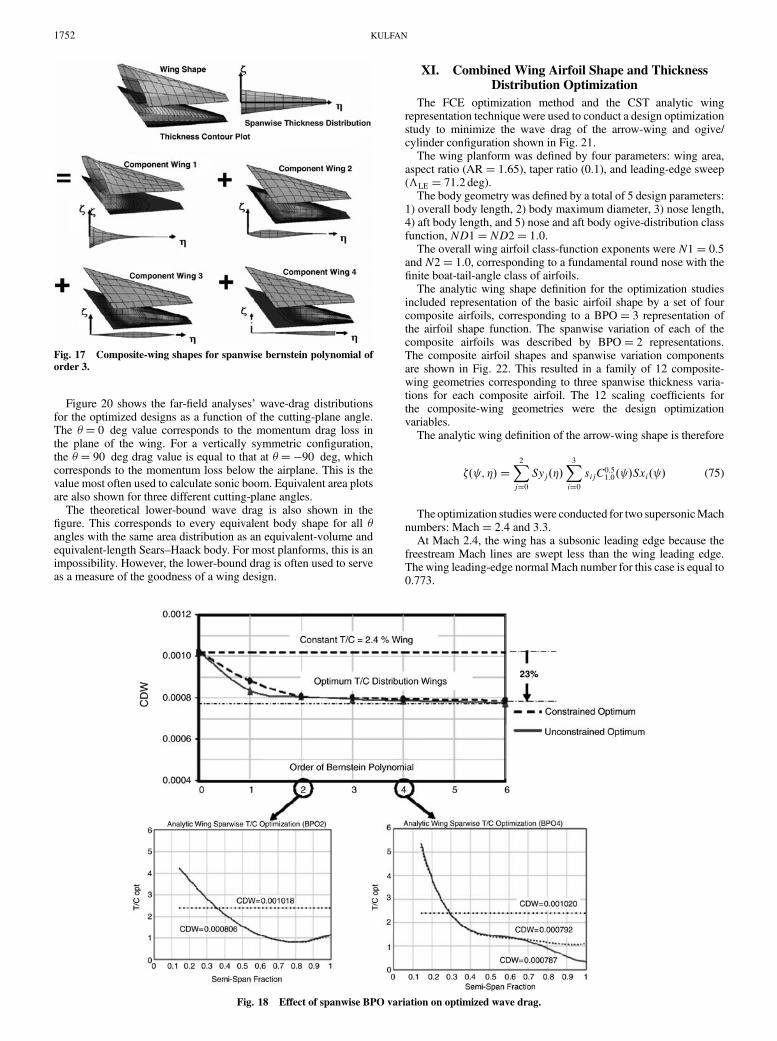
Figure 20 shows the far-field analyses’ wave-drag distributionsfor the optimized designs as a function of the cutting-plane angle.The �� 0 deg value corresponds to the momentum drag loss inthe plane of the wing. For a vertically symmetric configuration,the �� 90 deg drag value is equal to that at ���90 deg, whichcorresponds to the momentum loss below the airplane. This is thevalue most often used to calculate sonic boom. Equivalent area plotsare also shown for three different cutting-plane angles.

The theoretical lower-bound wave drag is also shown in thefigure. This corresponds to every equivalent body shape for all �angles with the same area distribution as an equivalent-volume andequivalent-length Sears–Haack body. For most planforms, this is animpossibility. However, the lower-bound drag is often used to serveas a measure of the goodness of a wing design.

XI. Combined Wing Airfoil Shape and ThicknessDistribution Optimization

The FCE optimization method and the CST analytic wingrepresentation techniquewere used to conduct a design optimizationstudy to minimize the wave drag of the arrow-wing and ogive/cylinder configuration shown in Fig. 21.

The wing planform was defined by four parameters: wing area,aspect ratio (AR� 1:65), taper ratio (0.1), and leading-edge sweep(�LE � 71:2 deg).

The body geometry was defined by a total of 5 design parameters:1) overall body length, 2) body maximum diameter, 3) nose length,4) aft body length, and 5) nose and aft body ogive-distribution classfunction, ND1� ND2� 1:0.

The overall wing airfoil class-function exponents were N1� 0:5and N2� 1:0, corresponding to a fundamental round nose with thefinite boat-tail-angle class of airfoils.

The analytic wing shape definition for the optimization studiesincluded representation of the basic airfoil shape by a set of fourcomposite airfoils, corresponding to a BPO� 3 representation ofthe airfoil shape function. The spanwise variation of each of thecomposite airfoils was described by BPO� 2 representations.The composite airfoil shapes and spanwise variation componentsare shown in Fig. 22. This resulted in a family of 12 composite-wing geometries corresponding to three spanwise thickness varia-tions for each composite airfoil. The 12 scaling coefficients forthe composite-wing geometries were the design optimizationvariables.

The analytic wing definition of the arrow-wing shape is therefore

�� ; �� �X2j�0

Syj���X3i�0

sijC0:51:0� �Sxi� � (75)

The optimization studieswere conducted for two supersonicMachnumbers: Mach� 2:4 and 3.3.

At Mach 2.4, the wing has a subsonic leading edge because thefreestream Mach lines are swept less than the wing leading edge.Thewing leading-edge normal Mach number for this case is equal to0.773.

Fig. 17 Composite-wing shapes for spanwise bernstein polynomial of

order 3.

Fig. 18 Effect of spanwise BPO variation on optimized wave drag.

1752 KULFAN

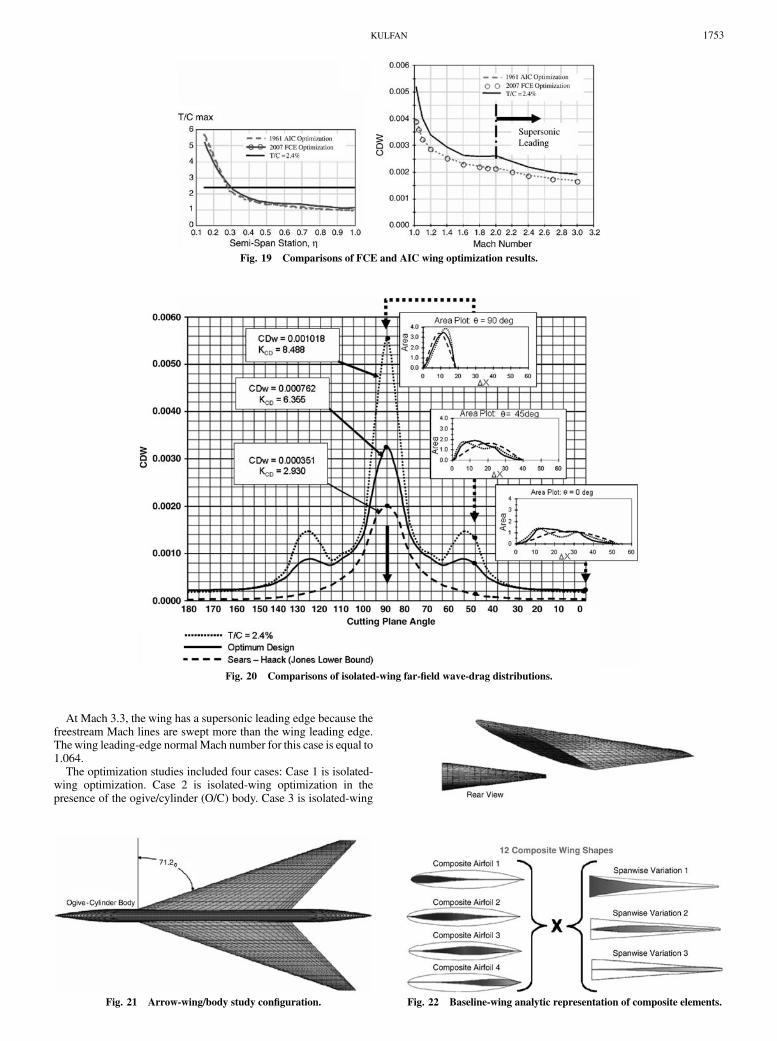
At Mach 3.3, the wing has a supersonic leading edge because thefreestream Mach lines are swept more than the wing leading edge.Thewing leading-edge normal Mach number for this case is equal to1.064.

The optimization studies included four cases: Case 1 is isolated-wing optimization. Case 2 is isolated-wing optimization in thepresence of the ogive/cylinder (O/C) body. Case 3 is isolated-wing

Fig. 19 Comparisons of FCE and AIC wing optimization results.

Fig. 20 Comparisons of isolated-wing far-field wave-drag distributions.

Fig. 21 Arrow-wing/body study configuration. Fig. 22 Baseline-wing analytic representation of composite elements.

KULFAN 1753

optimization with an outboard thickness. Case 4 is isolated-wingoptimization with an outboard thickness in the presence of the body.

The referencewing for the drag comparisons was an equal-volumewing with a constant-thickness/chord-ratio t=c biconvex airfoil. Thet=c was equal to 3.45%.

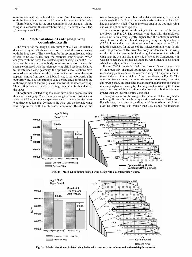
XII. Mach 2.4 Subsonic Leading-Edge WingOptimization Results

The results for the design Mach number of 2.4 will be initiallydiscussed. Figure 23 shows the results for of the isolated-wingoptimization, case 1. The wave drag for the optimum isolated-wingis seen to be 29.3% less than the reference configuration. Whenanalyzed with the body, the isolated optimum wing is about 23.4%less than the reference wing/body. Wing section airfoils across thespan are compared with the reference-wing airfoil sections. Relativeto the reference-wing geometry, the optimum airfoil sections haverounded leading edges, and the location of the maximum thicknessappears to move from aft on the inboard wing to more forward on theoutboard wing. The wing trailing-edge closure angle for most of theoutboard portion of the wing is less than that of the reference wing.These differences will be discussed in greater detail further along inthe paper.

The optimum isolated-wing thickness distribution becomes ratherthin near thewing tip. Consequently, awing thickness constraint wasadded at 95.2% of the wing span to ensure that the wing thicknesswould never be less than 2% across the wing, and the isolated-wingwas reoptimized with the thickness constraint. Results of the

isolated-wing optimization obtainedwith the outboard t=c constraintare shown in Fig. 24. Restricting thewing to be no less than 2% thickhad an extremely small effect on the wave drag of the optimum wingand on the optimum wing/body.

The results of optimizing the wing in the presence of the bodyare shown in Fig. 25. The isolated-wing drag with the thicknessconstraint is only very slightly higher than the optimum isolatedwing; however, the combined wing/body drag is slightly lower(23.6% lower) than the reference wing/body relative to 23.4%reduction achieved for the case of the isolated optimum wing. In thiscase, the presence of the favorable body interference on the wingresulted in an increase in the local wing thickness on the outboardwing near the trip and also at the side of the body. Consequently, itwas not necessary to include an outboard-wing thickness constraintwhen the body effects were included.

Figures 26–29 contain detailed comparisons of the characteristicsof the previously discussed optimized wing designs with the cor-responding parameters for the reference wing. The spanwise varia-tions of the maximum thickness/chord are shown in Fig. 26. Theoptimum isolated-wing tmax =c decreases continually over theentire wing span. This indicates that the nominal drag per unit area isrelatively high near thewing tip. The single outboard-wing thicknessconstraint resulted in a maximum thickness distribution that wasgreater than 2% over the entire wing span.

The optimization of the wing in the presence of the body had arather significant effect on thewingmaximum thickness distribution.For this case, the spanwise distribution of the maximum thicknessover the entire wing was greater than 2%. Hence, no thickness

Fig. 23 Mach 2.4 optimum isolated-wing design with a constant wing volume.

Fig. 24 Mach 2.4 optimum isolated-wing design with constant wing volume and outboard depth constraint.

1754 KULFAN

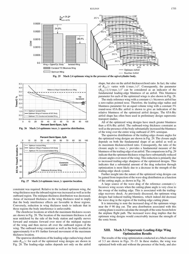
constraint was required. Relative to the isolated optimum wing, thewing thickness near the inboard regionwas increased aswell as in theoutboard region. The midspan thickness distribution was decreased.Areas of increased thickness on the wing thickness tend to implythat the body interference effects are favorable in those regions.Conversely, reduction in wing thickness tends to indicate that inthose regions the body interference is unfavorable.

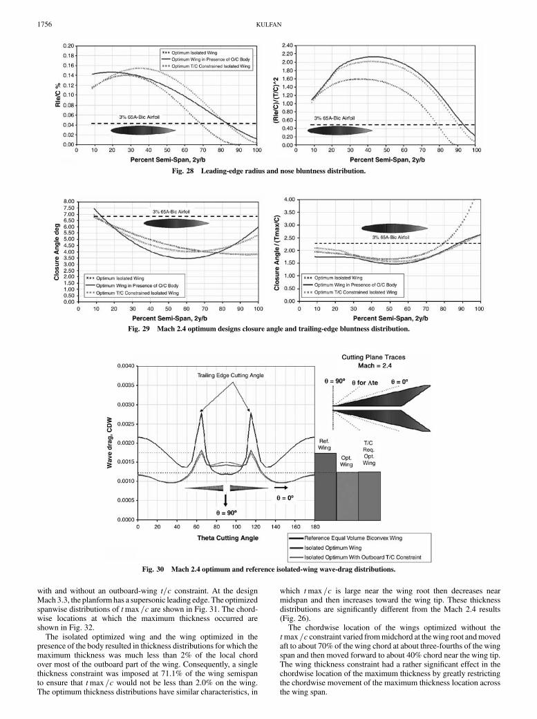
The chordwise locations at which the maximum thickness occursare shown in Fig. 28. The location of the maximum thickness is aftnear midchord by the side of the body station and rapidly movesforward and remains forward over most of the midspan regionsof the wing and then moves aft over the outboard region of thewing. The outboard-wing constraint as well as the body resulted inapproximately 6 to 8% further forward movement of the maximumthickness location.

The spanwise distributions of the leading-edge-radius/wing-chordratio RLE=c for each of the optimized wing designs are shown inFig. 28. The leading-edge radius depends not only on the airfoil

shape, but also on the airfoil thickness/chord ratio. In fact, the valueof RLE=c varies with �tmax =c�2. Consequently, the parameter�RLE=c�=�tmax =c�2 can be considered as an indicator of thefundamental leading-edge bluntness of an airfoil. This bluntnessparameter for each of the optimized wings is also shown in Fig. 28.

The study reference wing with a constant-t=c biconvex airfoil hasa zero-radius pointed nose. Therefore, the leading-edge radius andbluntness parameter for an equal-volume wing with a constant 3%round-nose 65A-Bic airfoil is shown to give an indication of therelative bluntness of the optimized airfoil designs. The 65A-Bicairfoil shape has often been used in preliminary design supersonictransport studies.

All of the optimized wing designs have much greater bluntnessthan a 65A-Bic airfoil. The outboard-wing thickness constraint aswell as the presence of the body substantially increased the bluntnessof the wing over the entire wing outboard of 20% semispan.

The spanwise distributions of the trailing-edge closure angles forthe optimized wing designs are shown in Fig. 29. The closure angledepends on both the fundamental shape of an airfoil as well asits maximum thickness/chord ratio. Consequently, the ratio of theclosure angle to tmax =c provides a fundamental measure of thebluntness of the trailing edge of an airfoil. The comparisons in Fig. 29indicate that the optimum thicknesswings have substantially reducedclosure angles over most of thewing. This reduction is primarily dueto increased trailing-edge sharpness of the optimized designs. Thisindicates that a substantial amount of the drag reduction throughoptimization is most likely due to a decrease in the strength of thetrailing-edge shock system.

Further insight into the nature of the optimized wing designs canbe gained from inspection of thewave-drag distribution as a functionof the cutting angle, as shown in Fig. 30.

A large source of the wave drag of the reference constant-t=cbiconvex wing occurs when the cutting-plane angle is very close tothe sweep of the trailing edge. This is associated with the trailing-edge recovery shock. As previously discussed, the optimum wingdesigns had reduced trailing bluntness, which indeed did decreasethe wave drag in the region of the trailing-edge cutting plane.

It is interesting to note the increased drag of the optimum wingsnear the � 90 deg cut. The area distribution associated with thiscutting plane is used to calculate the strength of the sonic boombelowthe airplane flight path. The increased wave drag implies that theoptimum wing designs would conceivably increase the strength ofthe sonic boom.

XIII. Mach 3.3 Supersonic Leading-Edge WingOptimization Results

The results of the wing optimization conducted at a Mach numberof 3.3 are shown in Figs. 31–33. In these studies, the wing wasoptimized both with and without the presence of the body, and also

Fig. 25 Mach 2.4 optimum wing in the presence of the ogive/cylinder body.

Fig. 26 Mach 2.4 optimum tmax =c spanwise distribution.

Fig. 27 Mach 2.4 optimum tmax =c spanwise location.

KULFAN 1755

with and without an outboard-wing t=c constraint. At the designMach 3.3, the planformhas a supersonic leading edge. The optimizedspanwise distributions of tmax =c are shown in Fig. 31. The chord-wise locations at which the maximum thickness occurred areshown in Fig. 32.

The isolated optimized wing and the wing optimized in thepresence of the body resulted in thickness distributions for which themaximum thickness was much less than 2% of the local chordover most of the outboard part of the wing. Consequently, a singlethickness constraint was imposed at 71.1% of the wing semispanto ensure that tmax =c would not be less than 2.0% on the wing.The optimum thickness distributions have similar characteristics, in

which tmax =c is large near the wing root then decreases nearmidspan and then increases toward the wing tip. These thicknessdistributions are significantly different from the Mach 2.4 results(Fig. 26).

The chordwise location of the wings optimized without thetmax =c constraint varied frommidchord at thewing root andmovedaft to about 70% of the wing chord at about three-fourths of the wingspan and then moved forward to about 40% chord near the wing tip.The wing thickness constraint had a rather significant effect in thechordwise location of the maximum thickness by greatly restrictingthe chordwise movement of the maximum thickness location acrossthe wing span.

Fig. 28 Leading-edge radius and nose bluntness distribution.

Fig. 29 Mach 2.4 optimum designs closure angle and trailing-edge bluntness distribution.

Fig. 30 Mach 2.4 optimum and reference isolated-wing wave-drag distributions.

1756 KULFAN

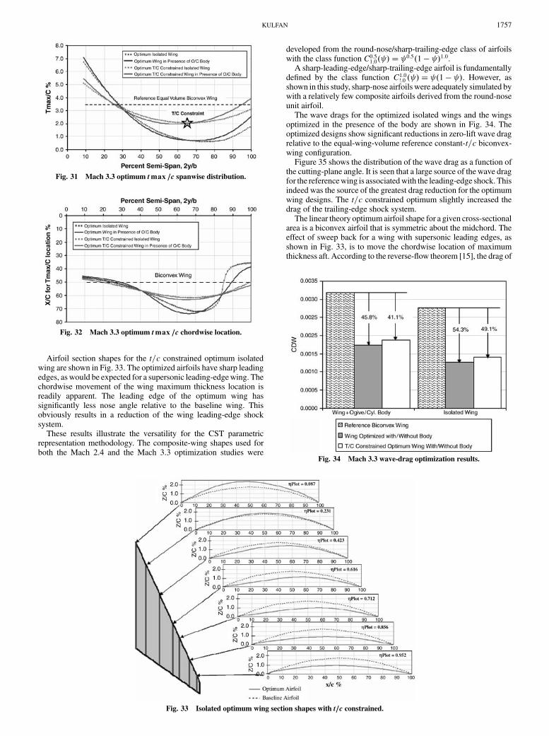
Airfoil section shapes for the t=c constrained optimum isolatedwing are shown in Fig. 33. The optimized airfoils have sharp leadingedges, as would be expected for a supersonic leading-edgewing. Thechordwise movement of the wing maximum thickness location isreadily apparent. The leading edge of the optimum wing hassignificantly less nose angle relative to the baseline wing. Thisobviously results in a reduction of the wing leading-edge shocksystem.

These results illustrate the versatility for the CST parametricrepresentation methodology. The composite-wing shapes used forboth the Mach 2.4 and the Mach 3.3 optimization studies were

developed from the round-nose/sharp-trailing-edge class of airfoilswith the class function C0:5

1:0� � � 0:5�1 � �1:0.A sharp-leading-edge/sharp-trailing-edge airfoil is fundamentally

defined by the class function C1:0!:0 � � � �1 � �. However, as

shown in this study, sharp-nose airfoils were adequately simulated bywith a relatively few composite airfoils derived from the round-noseunit airfoil.

The wave drags for the optimized isolated wings and the wingsoptimized in the presence of the body are shown in Fig. 34. Theoptimized designs show significant reductions in zero-lift wave dragrelative to the equal-wing-volume reference constant-t=c biconvex-wing configuration.

Figure 35 shows the distribution of the wave drag as a function ofthe cutting-plane angle. It is seen that a large source of the wave dragfor the referencewing is associatedwith the leading-edge shock. Thisindeed was the source of the greatest drag reduction for the optimumwing designs. The t=c constrained optimum slightly increased thedrag of the trailing-edge shock system.

The linear theory optimum airfoil shape for a given cross-sectionalarea is a biconvex airfoil that is symmetric about the midchord. Theeffect of sweep back for a wing with supersonic leading edges, asshown in Fig. 33, is to move the chordwise location of maximumthickness aft. According to the reverse-flow theorem [15], the drag of

Fig. 31 Mach 3.3 optimum tmax =c spanwise distribution.

Fig. 32 Mach 3.3 optimum tmax =c chordwise location.

Fig. 33 Isolated optimum wing section shapes with t=c constrained.

Fig. 34 Mach 3.3 wave-drag optimization results.

KULFAN 1757

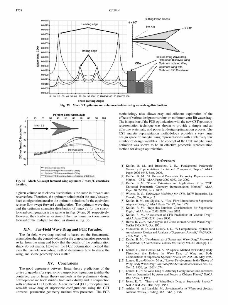
a given volume or thickness distribution is the same in forward andreverse flow. Therefore, the optimum solutions for the study’s swept-back configuration are also the optimum solutions for the equivalentreverse-flow swept-forward configuration. The optimum wave dragand the optimum spanwise distribution of tmax =c for the swept-forward configuration is the same as in Figs. 34 and 31, respectively.However, the chordwise location of the maximum thickness movesforward of the midspan location, as shown in Fig. 36.

XIV. Far-Field Wave Drag and FCE Paradox

The far-field wave-drag method is based on the fundamentalassumption that the control volume for the drag calculation process isso far from the wing and body that the details of the configurationshape do not matter. However, the FCE optimization method thatuses the far-field wave-drag method determines how to shape thewing, and so the geometry does matter.

XV. Conclusions

The good agreement between linear theory predictions of thecruise drag polars for supersonic transport configurations justifies thecontinued use of linear theory methods in the preliminary designdevelopment and trade studies, both individually and in conjunctionwith nonlinear CFD methods. A new method (FCE) for optimizingzero-lift wave drag of supersonic configurations using the CSTuniversal parametric geometry method was presented. The FCE

methodology also allows easy and efficient exploration of theeffects of various design constraints onminimumzero-lift wave drag.The integration of the FCE optimization with the newCST geometryrepresentation technique was shown to provide a simple and aneffective systematic and powerful design optimization process. TheCST analytic representation methodology provides a very largedesign space of analytic wing representations with a relatively fewnumber of design variables. The concept of the CST analytic wingdefinition was shown to be an effective geometric representationmethod for design optimization.

References

[1] Kulfan, B. M., and Bussoletti, J. E., “Fundamental ParametricGeometry Representations for Aircraft Component Shapes,” AIAAPaper 2006-6948, Sept. 2006.

[2] Kulfan, B. M., “A Universal Parametric Geometry RepresentationMethod—CST,” AIAA Paper 2007-0062, Jan 2007.

[3] Kulfan, B. M., “Recent Extensions and Applications of the ‘CST’Universal Parametric Geometry Representation Method,” AIAAPaper 2007-7709, Sept. 2007.

[4] Wilcox, D. C., Turbulence Modeling for CFD, DCW Industries, LaCanada, CA, 2006, p. 3.

[5] Kulfan, R. M., and Sigalla, A., “Real Flow Limitations in SupersonicAirplane Design:,” AIAA Paper 78-147, Jan. 1978.

[6] Kulfan, B. M., “Reynolds Numbers Considerations for SupersonicFlight,” AIAA Paper 2002-2839, June 2002.

[7] Kulfan, B. M., “Assessment of CFD Predictions of Viscous Drag,”AIAA Paper 2000-2391, June 2000.

[8] Harris, R. V., Jr., “AnAnalysis and Correlation of Aircraft Wave Drag,”NASATMX 947, Oct. 1961.

[9] Middleton, W. D., and Lundry, J. L., “A Computational System forAerodynamicDesign andAnalysis of Supersonic Aircraft,”NASACR-2715, Mar. 1976.

[10] Kulfan, B. M., “Fundamentals of Supersonic Wave Drag,” Reports ofthe Institute of Fluid Science, TohokuUniversity, Vol. 20, 2008, pp. 11–70.

[11] Lomax, H., and Heaslet, M. A., “A Special Method for Finding BodyDistortions that Reduce the Wave Drag of Wing and BodyCombinations at Supersonic Speeds,”NACARMA55B16, May 1955.

[12] Lomax, H., andHeaslet, M.A., “Recent Developments in the Theory ofWing-BodyWaveDrag,” Journal of the Aeronautical Sciences, Vol. 23,No. 12, 1956, pp. 1061–1074.

[13] Lomax, H., “The Wave Drag of Arbitrary Configurations in LinearizedFlow as Determined by Areas and Forces in Oblique Planes,” NACARM A55A18, 1955.

[14] Jones, R. T., “Theory of Wing-Body Drag at Supersonic Speeds,”NACA RM-A53H18a, Sept. 1953.

[15] Ashley, H., and Landahl, M., Aerodynamics of Wings and Bodies,Addison Wesley, Reading, MA, 1965, p. 196.

Fig. 35 Mach 3.3 optimum and reference isolated-wing wave-drag distributions.

Fig. 36 Mach 3.3 swept-forward wing optimum Tmax =C chordwise

location.

1758 KULFAN