Embed Size (px)
Citation preview

OPTIMIZATION OF SOLAR ENERGY HARVESTING: BUILDING
INFRASTRUCTURE AND STATISTICAL OPTIMIZATION
By
Zaid I. Almusaied
A thesis submitted to the Graduate Council of
Texas State University in partial fulfillment
of the requirements for the degree of
Master of Science in Technology
with a Major in Industrial Technology
May 2016
Committee Members:
Bahram Asiabanpour, Chair
Semih Aslan
Harold Stern
Farhad Ameri

COPYRIGHT
by
Zaid I. Almusaied
2016

FAIR USE AND AUTHOR’S PERMISSION STATEMENT
Fair Use
This work is protected by Copyright Laws of the United States (Public Law 94-553,
section 107). Consistent with fair use as defined in the Copyright Laws, brief quotations
from this material are allowed with proper acknowledgement. Use of this material for
financial gain without the author’s express written permission is not allowed.
Duplication Permission
As the copyright holder of this work I, Zaid I. Almusaied, authorize duplication of this
work, in whole or in part, for educational or scholar purpose only.

DEDICATION
I dedicate this thesis to my mother, Soad, whose memory has continually inspired me to
stay driven in the pursuit of my goals.

v
ACKNOWLEDGEMENTS
I would like to express deepest gratitude to my advisor Dr. Bahram Asiabanpour
for his full support, expert guidance, understanding and encouragement throughout my
study and research. Without his incredible patience and timely counsel, my thesis work
would have been a frustrating and overwhelming pursuit. I also express my appreciation
to Dr. Semih Aslan, Dr. Harold Stern, and Dr. Farhad Ameri for having served on my
committee. Their thoughtful questions and comments were valued greatly.
I would also like to thank Dr. Andy Batey, Dr. Cassandrea Hager and fellow
Engineering Technology faculty for helping me with my coursework and academic
research during my graduate years.
Finally, I would like to thank my father, Ibrahim Almusaied, for his
unconditional support during the last few years; I would not have been able to complete
this program without his continuous encouragement.
vi
TABLE OF CONTENTS
Page
ACKNOWLEDGEMENTS .................................................................................................v
LIST OF TABLES .......................................................................................................... viii
LIST OF FIGURES ........................................................................................................... ix
ABSTRACT ..................................................................................................................... xiii
CHAPTER
I. INTRODUCTION ..................................................................................................1
Background ..................................................................................................1
The History of Photovoltaic (PV) ................................................................3
Semiconductors ............................................................................................4
Acceptors Impurities ........................................................................6
Donors Impurities ............................................................................8
The p-n Junction ..........................................................................................9
The Photovoltaic Effect .............................................................................10
Photovoltaic Materials ...............................................................................16
Solar Electric System and Photovoltaic Cells Efficiency ..........................19
The Scope of the Research .........................................................................21
II. SOME SOURCES OF INEFFICIENCY IN SOLAR PANELS ..........................23
Power Conversion ......................................................................................23
Remedy ..........................................................................................23
Solar Panel Orientation and Tilting ...........................................................24
Remedy ..........................................................................................25
Temperature ..............................................................................................25
Remedy ..........................................................................................28
Dust and Dirt ..............................................................................................29
Remedy ..........................................................................................32
Aging and Degradation ..............................................................................33
Remedy ..........................................................................................34
Other Factors and Compounding Effects ...................................................34
III. ELECTRICAL COMPONENTS .........................................................................36
Photovoltaic Panels ....................................................................................36
Loads ..........................................................................................................39

vii
Calculating the Area of the PV Panel Using the
Reported Efficiency ...................................................................................40
IV. THE WEB-BASED DATA ACQUISITION SYSTEM ......................................41
Data Acquisition Network .........................................................................41
The eGauge ................................................................................................42
The RS485 Converter ................................................................................43
The Sunny Sensorbox ................................................................................44
RS485 Power Injector ................................................................................45
Ambient Temperature Sensor ....................................................................46
The PV Panel Surface Temperature Sensor ...............................................46
DC Current Transducers ............................................................................47
Router, Ethernet Cables, and Wires. ..........................................................48
V. MECHANICAL SYSTEM ..................................................................................49
Background and Implementation ...............................................................49
VI. RESPONSE SURFACE METHODOLOGY .......................................................62
Introduction ................................................................................................62
Factors Identification .................................................................................63
Factors Levels in Feasible Ranges ............................................................65
Design of Experiments ...............................................................................68
Conducting the Experiments ......................................................................70
Data Analysis .............................................................................................72
Optmization................................................................................................78
Investigation the Sun’s Postion and Its Effect
on the Optimum Point ................................................................................80
Efficiency Calculations ..............................................................................82
Validation ...................................................................................................84
VII. CONCLUSIONS AND FUTURE WORKS ........................................................85
Conclusions ................................................................................................85
Future Works .............................................................................................86
APPENDIX SECTION .....................................................................................................88
REFERENCES ................................................................................................................103

viii
LIST OF TABLES
Table Page
1. Energy gap ...................................................................................................................12
2. Various influential parameters .....................................................................................35
3. The PV electrical specifications ...................................................................................37
4. Mechanical specifications ............................................................................................38
5. The specifications of the rheostat ................................................................................39
6. Bill of materials............................................................................................................60
7. Parts list ........................................................................................................................61
8. The four uncoded factors with their three levels .........................................................67
9. The four coded factors with their three levels .............................................................67
10. The analysis of the data using Minitab .......................................................................73
11. Mintab optimization results .........................................................................................79
12. Validation sample of data ............................................................................................84

ix
LIST OF FIGURES
Figure Page
1. The energy of the sun .....................................................................................................2
2. Pure silicon atoms with their covalent bonds ................................................................5
3. The difference in band gap for insulator, metal, and semiconductor.............................6
4. The creation of holes. .....................................................................................................7
5. The creation of free electrons ........................................................................................9
6. The p-n junction. ..........................................................................................................10
7. Wavelength and energy................................................................................................13
8. A photovoltaic device consisting of p-n junction ........................................................14
9. Equivalent electrical circuit .........................................................................................15
10. The efficiency record ...................................................................................................18
11. Photovoltaic cell structures ..........................................................................................19
12. The two I-V curves .................................................................................................................. 26
13. Temperature effect on PV cell efficiency ................................................................................ 27
14. Solar-intensity reduction in response to dust deposition .............................................31
15. The PV panel used in the research ...............................................................................36
16. The IV diagrams ..........................................................................................................38
17. The rheostat used in the research .................................................................................39
18. The wiring diagram of the system used in the research ...............................................41
19. The eGauge ..................................................................................................................43

x
20. The Chiyu BF-430 .......................................................................................................44
21. The sunny sensor box...................................................................................................45
22. The power injector .......................................................................................................45
23. The ambient temperature sensor used in this research.................................................46
24. The temperature sensor ................................................................................................47
25. The DC current transducer ...........................................................................................47
26. Square tube draft ..........................................................................................................51
27. Base plate draft ............................................................................................................51
28. The caster draft ............................................................................................................51
29. Fixed base plate............................................................................................................52
30. Square tube adaptor plate .............................................................................................52
31. Square tube column......................................................................................................52
32. Sweeping mechanism pin ............................................................................................53
33. D-plate draft .................................................................................................................53
34. T-slot bar ......................................................................................................................53
35. The final assembly draft...............................................................................................54
36. Parts draft and list ........................................................................................................54
37. Various parts draft and how to assemble .....................................................................55
38. Water jet machine used in the production ....................................................................55
39. 3D printer used in the production ................................................................................56
40. Chop saw used in the production .................................................................................56

xi
41. SuperStruts ...................................................................................................................56
42. The rotating base plate used in the mechanical system ...............................................57
43. The square tube adaptor base used in the mechanical system .....................................57
44. The square steel legs assembled to fixed base plate and caster ...................................57
45. The T-slot plastic bolt adaptor used in the mechanical system ...................................58
46. The D-plate with several tilt angle settings ..................................................................58
47. The two D-plates attached to the PV panel holder structure .......................................59
48. The final assembly of the mechanical system ..............................................................59
49. General model of a process or system .........................................................................64
50. The process diagram of the experiment .......................................................................65
51. Minitab ................................................................................................................................... 68
52. Using Minitab to create Box-Bhenken design of RSM ..............................................69
53. Using Minitab GUI to select unblocked Box-Bhenken runs .......................................69
54. Using Minitab GUI to identify the high and low levels for each factor ......................69
55. Using Minitab GUI to select the design specifications ................................................70
56. The PV panel with levels of treatments .......................................................................70
57. The PV panel subjected to the treatment during the experiment .................................71
58. Using the Minitab GUI to analyze the results ..............................................................72
59. Four-in-one residual plot generated by Minitab ..........................................................74
60. The main effect plot generated using Minitab for the yield response ..........................75
61. The surface plot of the yield response as generated using Minitab .............................76

xii
62. The interaction plot ......................................................................................................76
63. Contour plot of the yield response ...............................................................................77
64. The optimization graph generated by Minitab .............................................................80
65. The main effect for the runs before mid-day ...............................................................81
66. The main effect plot for the runs in the afternoon .......................................................82
67. The received irradiance for the two PV panels ............................................................83
68. The various recorded efficiency of the two PV panels during the experiment ............84

xiii
ABSTRACT
Renewable energy is the path for a sustainable future. The development in this
field is progressing rapidly and solar energy is at the heart of this development. The
performance and efficiency limitations are the main obstacles preventing solar energy
from fulfilling its potential. This research intends to improve the performance of solar
panels by identifying and optimizing the affecting factors. For this purpose, a mechanical
system was developed to hold and control the tilt and orientation of the photovoltaic
panel. A data acquisition system and electrical system were built to measure and store
performance data of the photovoltaic panels. A design of experiments and response
surface methodology were used to investigate the impact of these factors on the yield
response as well as the output optimization. The findings of the experiment showed an
optimum result with a tilt of 60º from the horizon, an azimuth angel of 45º from the south
and a clean panel condition. The wind factor showed insignificant impact within the
specified range. This work can be continued by investigations on the materials, geometry,
cleaning and cooling systems, and involving some other environmental and physical
factors.

1
I. INTRODUCTION
Background
The relation between man and the sun is ancient. The sun has played a massive
role in the history of mankind. Some old civilizations even had spiritual belief in the
power of the sun. According to Hsieh (1986), the sun is a giant nuclear reaction that
transforms four million tons of hydrogen to helium per second. The earth will receive
only a tiny amount of the sun generated energy (Hsieh, 1986). The radiated energy from
the sun must be equal to the energy it produces to ensure its structural stability (Sorensen,
2011). The evidence of this stability over the last 3 billion years can be seen by the
relative stability of the temperature of the earth’s surface (Sorensen, 2011). Oxidized
sediments and fossil remains reveal that the water fluid phase has been presented through
this time (Sorensen, 2011). The earth’s orbit around the sun is slightly elliptical, making
the distance between the two vary throughout the year. The earth and sun are 91.4 million
miles apart in January compared to 94.5 million miles in July; this leads to an annual
disparity of 3%–4% in the irradiance at the edge of the atmosphere (Shepherd &
Shepherd, 2014). Although the earth receives just a tiny fraction of the Sun’s generated
energy, it is still a massive amount of energy. The earth’s radiation reception rate is 1.73
* 1017 J/s, and in a year made up of 365.25 days, the total amount of radiation is 5.46 *
1024 J (Shepherd & Shepherd, 2014). Boylestad and Nashelsky (1989) stated that the
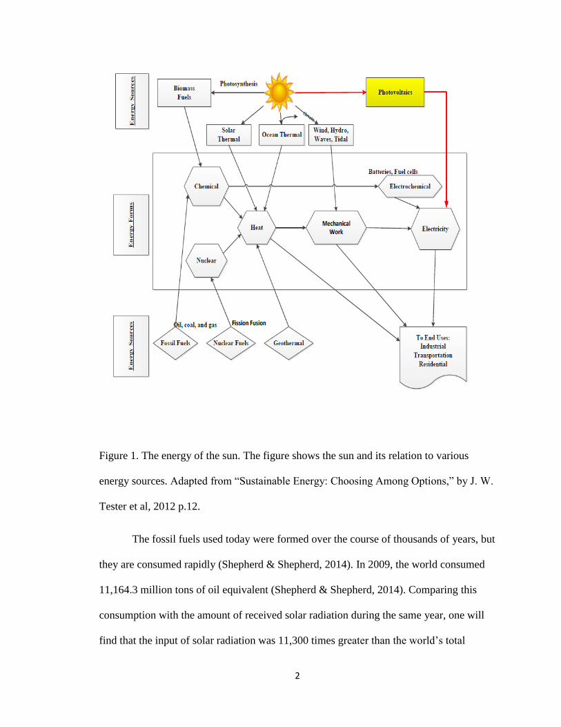
received energy at sea level is about 1 kW/m2. There are strong links of all known forms
of energy resources to the sun and how they are used by mankind (Tester, Drake,
Driscoll, Golay, and Peters, 2012; See Figure 1).
2
Figure 1. The energy of the sun. The figure shows the sun and its relation to various
energy sources. Adapted from “Sustainable Energy: Choosing Among Options,” by J. W.
Tester et al, 2012 p.12.
The fossil fuels used today were formed over the course of thousands of years, but
they are consumed rapidly (Shepherd & Shepherd, 2014). In 2009, the world consumed
11,164.3 million tons of oil equivalent (Shepherd & Shepherd, 2014). Comparing this
consumption with the amount of received solar radiation during the same year, one will
find that the input of solar radiation was 11,300 times greater than the world’s total
3
primary energy consumption (Shepherd & Shepherd, 2014). This increase in
consumption of the limited fossil fuel resources, the environmental concerns, plus the
fluctuations in the oil market have led humanity to search for more clean and renewable
sources of energy. For a long time, solar energy has been one of the most promising,
sustainable energy sources. Generating electricity from the incident light has many
challenges, and one of the greatest challenges is the drop in efficiency.
The History of Photovoltaic (PV)
The word photovoltaic is composed of two parts. The first is photo, which comes
from the Greek word φῶς (phōs) meaning light, and the second is volt, which comes from
the Italian scientist, Alessandro Volta, who invented the battery (electrochemical cell)
(Smee, 1849). Volt is the unit measurement of the electromotive force .Using
semiconductor materials to directly convert the solar energy into electricity is called
photovoltaic (Prasad, 2011). This effect was first discovered in 1839 by the French
physicist Edmund Becquerel in an electrolytic cell exposed to light (Prasad, 2011). In
1877, Adams and Day detected the effect in solid selenium (Bube, 1960) as cited by
(Goswami, Kreith, & Kreider, 2000). The progress in this field continued in 1904 when
Albert Einstein published a paper on the photoelectric effect (Prasad, 2011). This paper
led to Einstein being awarded the Nobel Prize for physics and drew more attention to this
field. (“The Nobel prize”, n.d.).
The competition between the United States of America and the Soviet Union to
reach outer space during the Cold War helped to escalate the attention to this field as
solar energy can be used to energize satellites, space stations, and vehicles to name a few.
The research done by Bell Laboratories and RCA in 1954 achieved efficiency up to six

4
percent. They used devices made of p and n types of semiconductors (Bube, 1960) as
cited by (Goswami, Kreith, & Kreider, 2000). The efficiency of solar panels has
improved since then, but efficiency is still considered one of the biggest sources of
limitation for the advancement of solar energy harvesting.
Semiconductors
Semiconductors are materials with conductivity between insulators and
conductors. Semiconductors such as silicon, germanium or gallium-arsenide will be
insulators with a relatively narrow energy gap (0.1 eV<Eg<3 eV) at low temperatures and
pure chemical condition (Kaltschmitt & Rau, 2007). Silicon and germanium lie in the
fourth column of the periodic table. As the nucleus of the atom will contain the positively
charged protons plus the uncharged neutrons, the negatively charged electrons will orbit
around the nucleus. The electrons have four quantum numbers (shell, subshell, orbital,
and spin). The quantum numbers describe the energy level, distance from the nucleus,
angular momentum, orbitals, and spin. The electrons are fermions that will have discrete
energy levels with no two electrons having the same four quantum number (Pauli
Exclusion Principle). The electrons that are farthest from the nucleus are the highest in
energy level. The valence layer (shell) is the outer layer. A silicon valence layer has four
electrons. These electrons will form tight covalent bonds with the neighboring atom’s
valence electrons. Thus, a pure crystal of material will be formed. A high energy will be
required to free an electron from the bond and make it a charge carrier. This makes the
pure semiconductor materials act as an insulator with low conductivity at room
temperature (Shepherd & Shepherd, 2014). Applying a voltage across such material at

5
room temperature will cause only a tiny amount of current (leakage current) to pass
through (Kaltschmitt & Rau, 2007).
Figure 2. Pure silicon atoms with their covalent bonds. Adapted from “Electricity and
Electronics a Survey,” (3rd ed.), by D. R. Patrick, & W. Stephen, 1996 p.246.
The electrons in the valence band, when energetic, will jump to a higher band.
The higher band is called a conduction band where a small amount of impressed force
would release the electrons from the atom. These electrons are responsible for the
conduction of heat and electricity. The energy distinction between a valence electron and
the inner subshell of the conduction band is called a band gap. Insulators have high band
gaps (>3 eV) (Goswami et al., 2000).

6
Figure 3. The difference in band gap for insulator, metal, and semiconductor. The
insulator, a., with the bigger band gap and empty conduction band. The conductors, b.
Metal, have a small band gap and sometimes there will be an overlap between the valence
and conduction band. The conduction band is partly filled with electrons. The
semiconductor, c., has a moderate band gap and has a partially filled valence band.
Adapted from “Principle of Solar Energy,” by D. Y. Goswami, F. Kreith, and J. F.
Kreider, 2000 p. 414.
To increase the conductivity of the pure semiconductors, impurities are added to
them. Bell Telephone Laboratories in New Jersey, U.S.A., introduced this technology in
the 1950s (Shepherd & Shepherd, 2014). We can categorize impurities into two groups:
Acceptors Impurities
Materials from the third column of the periodic table like boron, aluminum,
gallium, and indium will be used to dope the pure semiconductor materials. These
materials, the impurities, have three electrons in their outer shells. The acceptor
impurities have their name because they can accept free electrons. The impurity atoms
constitute three covalent bonds with their neighboring atoms using their three outer

7
electrons. This will lead to a hole forming at the fourth side, as the covalent bond with the
adjacent pure semiconductor atoms will lack the necessary electron. Applying potential
difference across the doped semiconductors will result in migration of holes. This kind of
doping forms a p-type, positive, semiconductor. The holes are the majority of the charge
carriers. The free electrons are the minority of the charge carriers (Shepherd & Shepherd,
2014).
Figure 4. The creation of holes. The silicon atoms share their four valence electrons with
their neighbors creating covalent bonds. When impurities from the third column of the
periodic table are doped into the silicon they will create covalent bonds with the silicon
atoms, but having only three electrons on their outer shell a hole will be created. Adapted
from “Energy studies,” by W. Shepherd and D.W. Shepherd, 2014 p. 430.

8
Donors Impurities
Materials from the fifth column of the periodic table, such as arsenic, phosphorus,
and antimony, will be used to dope the pure semiconductors. These materials, the
impurities, have five electrons in their outer shells. The impurity atom constitutes four
covalent bonds with its neighboring atoms using its four outer electrons. This will leave
the fifth electron of the impurity atom to lie in the valence shell. Such an electron can be
easily freed from his original atom when applying electromotive force to the doped
semiconductor. These impurities are called donors because they can supply free
electrons. This kind of doping forms an n-type, negative, semiconductor. The free
electrons are the majority of the charge carriers. The holes are the minority of the charge
carriers (Shepherd & Shepherd, 2014).
9
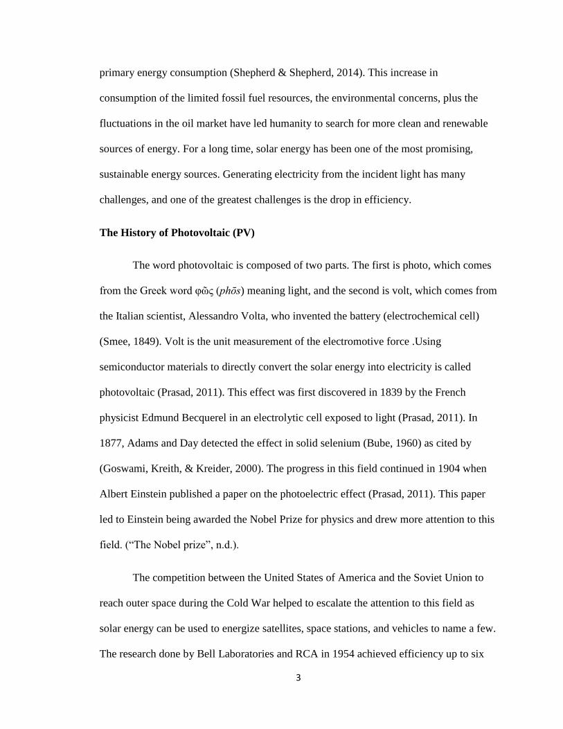
Figure 5. The creation of free electrons. The silicon atoms share their four valence electrons
with their neighbors creating covalent bonds. When impurities from the fifth column of the
periodic table are doped into the silicon they will create covalent bonds with the silicon
atoms, but having five electrons on their outer shell free electrons will be excess. Adapted
from “Energy studies,” by W. Shepherd and D.W. Shepherd, 2014 p. 430.
The p-n Junction
The characteristic of the n-type materials will lead to an excessive amount of free
electrons, while the p-type materials have, the opposite, holes. When contacting these two
materials, the free electrons from the n-layer will jump to fill the holes in the p-layer.
This situation will result in positive charges on the n-layer near the junction. The negative
charges will be on the p-layer near the junction (Goswami et al., 2000). As a result of the
carriers’ movement, an electrical field will be formed on the sides of the junction and
thus a depletion area will be established (Kaltschmitt & Rau, 2007).

10
Figure 6. The p-n junction. The p-type material has an excess of holes while the n-type
material has an excess of electrons. When they are attached together the electrons will
move from the n-type toward the p-type while the holes will move from the p-type
toward the n-type. The movements will continue until an electric field will be created due
the accumulation of electrons on the p side of the junction and holes on the n side of the
junction creating a depletion region. Adapted from “Principle of Solar Energy,” by D.
Y. Goswami, F. Kreith, and J. F. Kreider, 2000 p. 415.
The Photovoltaic Effect
According to Kaltschmitt and Rau (2007), as the light photon reaches the atom
valence electron it will be absorbed by it. The absorption increases the electron’s energy.
When the photon’s energy is equivalent or more than the energy band gap of the
semiconductors, the electron will move to the conduction band. If the absorbed energy is
less, the extra energy will transform into kinetic energy. Also, if the absorbed photon is
more than what is needed to cross the energy band gap, as one photon can free only one

11
electron, the extra energy will also convert into kinetic energy. In both cases, the kinetic
energy will manifest itself as heat (Kaltschmitt & Rau, 2007). This phenomenon is a
major player in the conversion efficiency of photovoltaic devices.
The photon is a quantum of energy, as defined by Max Planck, and can be calculated by
his equation
𝐸𝑝= hv
Where h is Planck’s constant (6.625 * 10−34 J.sec), (𝑣) is the frequency. The frequency
can be represented by its associated wavelength (λ) and light speed (c) by using the
equation:
𝑐 = 𝑣𝜆
𝑣 = 𝑐
𝜆
𝐸𝑝 =ℎ𝑐
𝜆
From the above equation and for silicon, which has a band gap of 1.11eV, we can
calculate the wavelength of light that is capable of forming an electron-hole pair. This
wavelength is 1.12 𝜇m or less (Goswami et al., 2000).
12
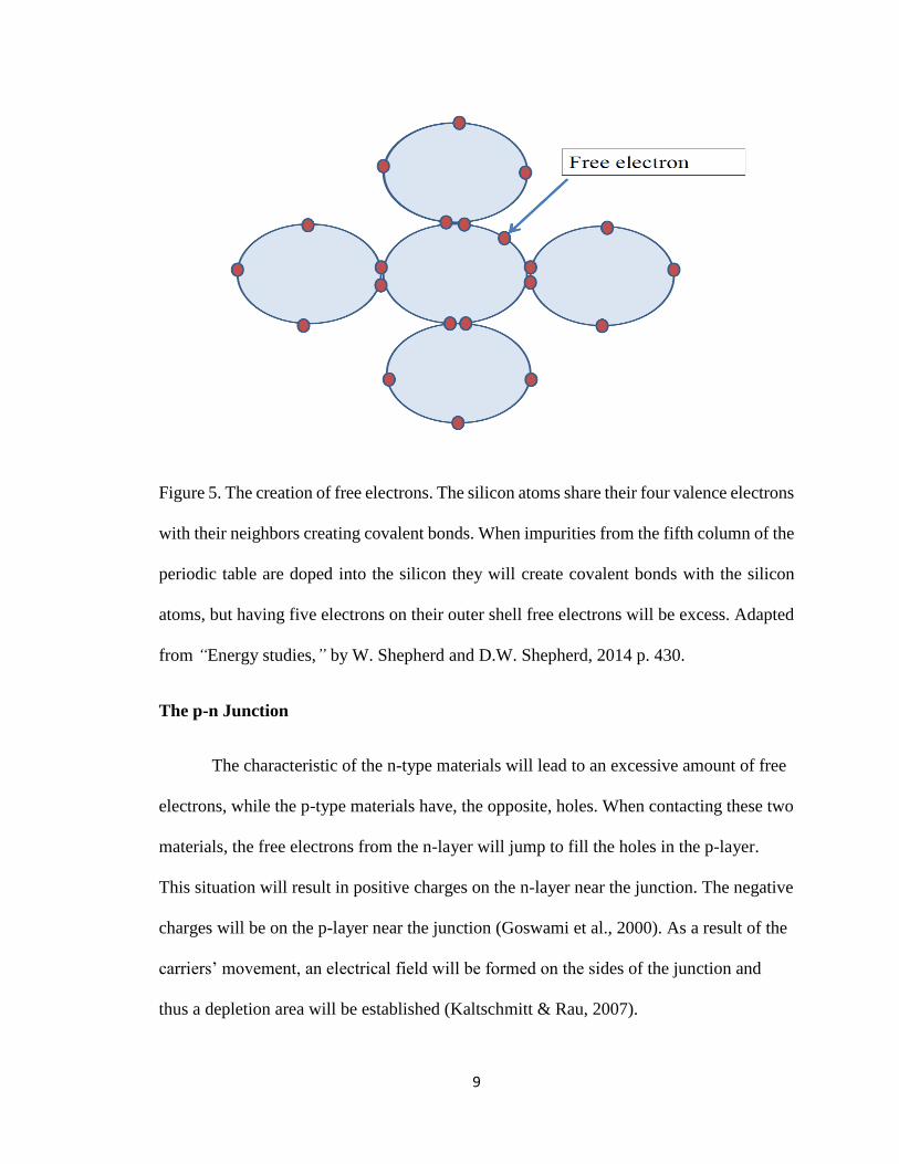
Table 1. Energy gap. Various energy gaps for materials that can be used for photovoltaic
cells. Adapted from “Principles of Solar Engineering,” by D. Y. Goswami, F. Kreith, and
J. F. Kreider, 2000, p. 417.
Material Band gap (eV) Material Band gap (eV)
Si 1.11 CuInT𝑒2 0.90
SiC 2.60 InP 1.27
CdA𝑠2 1.00 I𝑛2T𝑒3 1.20
CdTe 1.44 I𝑛2𝑂3 2.80
CdSe 1.74 Z𝑛3𝑃2 1.60
CdS 2.42 ZnTe 2.20
CdSn𝑂4 2.90 ZnSe 2.60
GaAs 1.40 AIP 2.43
GaP 2.24 AISb 1.63
C𝑢2S 1.80 A𝑠2S𝑒3 1.60
CuO 2.00 S𝑏2 S𝑒3 1.20
C𝑢2Se 1.40 Ge 0.67
CuIn𝑆2 1.50 Se 1.60
CuInS𝑒2 1.01

13
Figure 7. Wavelength and energy. The silicon photovoltaic cell uses only the photons that
have certain wavelengths that will result on an energy equal to or above the silicon band
gap. Adapted from “Solar Energy Engineering,” by S. Hsieh, 1986, p. 375.
The solar cell has a thin layer of n-type semiconductor, around 0.2 𝜇𝑚, attached
to a thicker layer of p-type semiconductor, around 300 𝜇𝑚 (Hsieh, 1986). The
photovoltaic effect will result in the uses of the freed electrons through the connection
terminals that connect the solar cell with the outer external resistance load to drive these
freed electrons outside the p-n junction before they unite with the holes (Goswami et al.,
2000).

14
Figure 8. A photovoltaic device consisting of p-n junction. The photovoltaic effect
happens when the solar radiation reaches a semiconductor and causes the separation of
the positive and negative charge carriers. When connectors contact the photovoltaic
device those carriers are driven out to external loads before recombination happens.
Adapted from “Principle of Solar Energy,” by D. Y. Goswami, F. Kreith, and J. F.
Kreider, 2000, p. 416.
The photovoltaic cell has an electrical equivalent of a current source, diode
with 𝑅𝑠ℎ𝑢𝑛𝑡, and 𝑅𝑠𝑒𝑟𝑖𝑒𝑠.

15
Figure 9. Equivalent electrical circuit. The photovoltaic cell can be replaced with an
equivalent electrical circuit, (a), of a current source, diode, internal parallel shunt
resistance, and internal series resistance. The internal shunt resistance is usually very
much higher than the external load so that the load will have most of the current, while
the series resistance is much less than the external load to ensure the minimum
dissipating of energy in it. More practical drawing of the equivalent circuit, (b), will be
without the shunt and series internal resistance. Adapted from “Solar Energy
Engineering,” by S. Hsieh, 1986, p. 376.

16
Where: 𝑅𝑠𝑒𝑟𝑖𝑒𝑠 is the internal resistance, 𝑅𝑠ℎ𝑢𝑛𝑡 is the internal parallel shunt resistance,
𝑅𝑗 is Junction resistance, 𝐼𝑠 is the light dependent current from the equivalent current
source, 𝐼𝑗 is the junction current, T is the absolute temperature in kelvin, and K is
Boltzmann's constant
Ij =Io [exp (eV
KT) – 1]
I𝑜 is the saturation current, also known as leakage or diffusion current.
I=Is - Ij
I=Is - Io [exp (eV
KT) – 1]
Photovoltaic Materials
The most common photovoltaic modules, or panels, in the market are based on
silicon. These photovoltaic panels vary in the way the silicon is manufactured (Prasad,
2011). Amorphous silicon cells are formed using uncrystallized silicon. No expensive
production techniques are required (Shepherd & Shepherd, 2014). They are often named
as thin silicon film, and this thin layer will be placed on various surfaces, such as glass.
The color will be usually dark matte (Prasad, 2011). The efficiency for this kind of
photovoltaic cell is low (typically 5-8%) (Prasad, 2011). Monocrystalline solar cells are
thin wafer. The wafer is cut from a large single crystal; thus it is expensive and uses a lot
of silicon (Shepherd, 1975). The cells are bluish-black in color (Prasad, 2011). According
to Menzies (1998) as cited by (Prasad, 2011), the efficiency is the best for such cells for a
given module area and the cells will have a long life when well manufactured.

17
Polycrystalline solar cells came as development in the manufacturing process. Prasad
(2011) stated that the cells are thin wafers cut from multiple crystal silicon. They are
distinguished by their blue color, but they could be another color. These cells are the
most common panels on the market. Two-thirds of the installed photovoltaic cells used
crystalline silicon in 2009, but the use of thin film technologies is steadily increasing EIA
(2010) as cited in (Tester et al., 2012). Choosing between polycrystalline and
monocrystalline is a tradeoff between cost and efficiency (Tester et al., 2012).
Many materials other than silicon have been investigated to determine their cost
and efficiency (Tester et al., 2012). Photovoltaic cells made of 1-3µm layers copper
indium diselenide (CuInSe₂or CIS), with thin over layers of silica (Si𝑂2) and cadmium
zinc sulfide (CdZnS) or cadmium sulfide (CdS) all have higher efficiency than silicon
based photovoltaic devices with similar manufacturing cost (Tester et al., 2012). CIS
cells have serious sustainability and toxicity problems. For example, the protection of the
workers, the environmental impact of the mining for elements like Zn, In, Mo, Se, Cd,
and Cu, and the end-of-life disposal should be considered during the manufacturing
process. This can also affect the regional supply and demand for these materials and raise
the cost (Tester et al., 2012).
Cadmium telluride (CdTe) is also a very promising material to use. It has an
energy band gap of 1.5 eV. This will make it very suitable for the solar spectrum. This
material has the same issues and concerns as the CIS; it may harm the environment, the
workers, and lead to resource depletion. Nevertheless, it is very promising especially with
improvement in manufacturing technology and reducing the cost with better efficiency
(Tester et al., 2012).

18
Figure 10. The efficiency record. The efficiency of different materials with different
technologies as it improves and reported every year. Adapted from “Efficiency Chart” by
National Renewable Energy Laboratory,” 2015.

19
Solar Electric System and Photovoltaic Cells Efficiency
Shepherd and Shepherd (2014) stated that photovoltaic cell structures can be
formed by connecting cells together to constitute a module, and modules are connected to
establish an array
Figure 11. Photovoltaic cell structures. Cells connected together to form a module, and
modules connected together to form an array. Adapted from “Energy studies,” by W.
Shepherd and D.W. Shepherd, 1975 p. 428.

20
` Solar electric systems can be categorized into three group according to Chiras
(2011): grid-connected, grid-connected with battery backup, and off-grid (Chiras, 2011).
The performance of solar cells and modules can be calculated through their efficiency.
The efficiency and some of the causes of losses stated by Prasad (2011) include
● Losses due to the collecting metallic grid that covers the surface of the
photovoltaic cell; this grid is responsible of collecting the electrons that the
photovoltaic effect will produce.
● Losses due to reflection; some of the sun’s radiation will be reflected from the
surface of the cell.
● Losses due to the combination of the freed electrons by the photovoltaic with the
holes in the semiconductors.
● Losses due to insufficient energy absorbed by the electrons to cross the energy
band gap. On the other hand, if the photon absorbed by the electron is more than
the required energy, the extra energy will be converted to heat.
● Losses due to shading of the photovoltaic cell, a drop in voltage will occur when
part of the cell or the module is shaded.
By reviewing some of the sources of losses we can conclude these sources are
inherent in the materials used to manufacture the cells or modules. The solar electrical
system components also will be a source of losses. These components are power
connections, inverters, control and interconnection equipment, and batteries (Tester et al.,
2012).

21
The Scope of the Research
The future of the solar energy depends on improving both the efficiency and
performance of the PV panels. The performance and efficiency of the PV panels depend
on many factors such as:
The manufacturing and material specifications where the maximum theoretical
efficiency is limited
Improving the power conversion for the PV panels systems, where the conversion
from the generated DC to AC causes losses in efficiency
Environmental factors (e.g. temperature, wind )
Status of the PV panels (e.g. orientation, tilting)
In this research the focus is on the environmental factors and status of the PV
panels where the designated location and time/date play a significant role on the
performance of the PV panels. The purposes of the research are to identify the significant
factors, their range, and the optimum settings to improve the performance of the PV
panel. The controllable factors include tilt, orientation (azimuth), wind, and the level of
cleanness.
Suitable infrastructure to conduct this research has been developed. The
infrastructure includes a mechanical system, an electrical system, and a web-based data
acquisition system. The experiment was designed and analyzed using response surface
methodology and design of experiments.
The first limitation for this research includes the limited number of PV panels
with the proper infrastructure to conduct the runs in the same time. Instead, a single panel

22
was utilized for all runs. This way, sun irradiance varies during the experiment, although
the use of the secondary solar panel in the flat position and clean status as the control
sample (not subject to treatment) and difference between power generations in two panels
eliminated the irradiance variability. Other limitations include uncontrollable factors
associated with the temperature and general weather conditions. Date, time, and
designated location can be considered as the delimitations. The study focuses on the
aforementioned controllable factors and their three levels of treatment.

23
II. SOME SOURCES OF INEFFICIENCY IN SOLAR PANELS
In this chapter, the sources of inefficiency in solar panels and the available
remedies are discussed.
Power Conversion
Photovoltaic (PV) panels produce a direct current (DC) as result of the
photovoltaic effect. The direct current needs to be converted into an alternating current
(AC) in order to connect to a utility grid or home appliances. Some systems use central
inverters for all panels in one location while other systems have a single inverter for each
PV panel. The process of converting direct current electricity into alternating current
electricity causes losses in efficiency. Many commercial inverters are available with
various levels of efficiency; some are up to 96%–98% while others might be less than
95% efficient. Inverters are significantly less efficient when used at the low end of their
maximum power. Many inverters are most efficient in the 30%–90% power range
(Central Electricity Regulatory Commission., 2011).
Remedy
Micro-inverters have several advantages, according to their producers. In addition
to having alternating current directly from each PV panel, a 5%-25% increase in power
output is typical for micro-inverters when compared to traditional PV panels utilizing
central inverters (GreenRay, Inc., 2010). Furthermore, micro-inverter manufacturers
claim that by having inverters decentralized, the system will be easier to install and
maintain with 40% fewer components. The micro-inverter seems promising, but as
Daniel Sullivan states (2012), the concept of having an electronic device exposed to
weather conditions may affect its performance and reliability.

24
There have been many attempts to directly obtain alternating current electricity
from solar panels. These attempts were found in different U.S. patents. Although they
succeeded in getting the alternating current directly from the PV panels, they couldn’t
achieve practical, reliable, or even an equal-in-efficiency system performance compared
to the use of inverters. This can be seen in the following patents (U.S. Patent No.
4,075,034, 1978), (U.S. Patent No. 4,577,052, 1986), (U.S. Patent No.4, 728,878, 1988),
(U.S. Patent No. 6,774,299, 2004), (U.S. Patent No. 2005/0034750, 2005), (U.S. Patent
No. 2010/0139735, 2010), (U.S. Patent No. 8,492,929 B2, 2013).
Solar Panel Orientation and Tilting
The orientation of the panel has an impact on its performance. The angle and
direction of the tilt is important to receive the incident insolation and generate electricity
from the PV panels. At the same time, orientation has another impact on the
accumulation of dust and dirt on the panel’s surface. The geographic location plays a
great role in determining the orientation. Common belief states that the PV panel’s
appropriate tilt angle should be the same as the latitude of the PV panel location on earth
(Mondol, Yohanis & Norton, 2007). It should be tilted (if the PV panel location is above
the equator) southward and toward the sun. Yet, some places have diverse weather
conditions with winters that are cloudier than summer, or the average morning and
afternoon insolation is not identical (Mondol et al., 2007). The result will be more energy
received by the PV panels when the azimuth angle is either east or west of due south (for
locations above the equator) (Mondol et al., 2007).

25
Remedy
To maximize the received incident insolation, it is best to have a tracking system
that will follow the sun to obtain the best result with perpendicular solar radiation flux on
the surface of the PV panel. Many commercial tracking systems are available. These
systems are either single or dual axis trackers (Neitzel, 2016). Having a sun tracker will
provide a better output but is also more expensive. Fixed PV panels with the appropriate
tilt for a specific location (optimum tilt angle is site dependent) can produce quality
energy (Mondol et al., 2007). Another aspect to consider is the season. To maximize the
incident insolation on the surface during summer, an inclination of 10°–15° less than the
latitude is usually required compared to 10°-15° more during winter (Duffie & Beckman,
1991) as cited by (Mondol et al., 2007).
Temperature
The efficiency of PV panels will be affected by the operating temperature. The
standard operating temperature for PV panels is 25° C with 1000 W/m2 of solar flux (Al-
Sabounchi, 1998). PV panels, like all other semiconductor devices, are sensitive to
temperature. The gain in temperature decreases the band gap, and that will decrease the
open circuit voltage (Voc). The maximum power is provided by the following equation:
Pm = Vm Im = (FF) Voc Isc (1)
The fill factor (FF in Equation 1) will also decrease substantially with the increase
in temperature. The short-circuit current will increase slightly (ZONDAG, 2007) as cited
by (Skoplaki & Palyvos, 2009).
ηc = ηTref [1-βref(Tc-Tref)+γlog10GT] (2)

26
Equation 2 defines the crystalline silicon efficiency where ηTref is the module’s
electrical efficiency at the reference temperature, Tref, and at solar radiation flux of 1000
W/m2. The temperature coefficient, βref, and the solar radiation coefficient, γ, are mainly
material properties, having values of about 0.004 K-1 and 0.12, respectively, for
crystalline silicon modules. The temperature coefficient (βref) is usually supplied by the
manufacturer, along with ηTref. The solar radiation coefficient γ is usually set to zero and
then Equation (2) is reduced to Equation (3) (Skoplaki & Palyvos, 2009).
ηc = ηTref [1-βref(Tc-Tref)] (3)
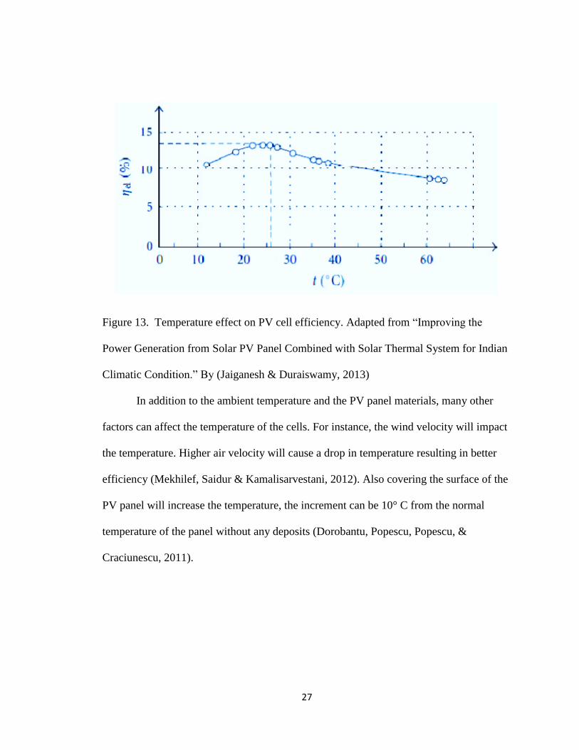
Figures 12 and 13 show the effect of temperature on voltage outputs and on the
cell efficiency, respectively. It is clear from Figure 12 that the voltage output is higher at
colder temperatures. Figure 13 shows that the PV cell efficiency is decreased as the
temperature is increased over the standard operating temperature of 25° C.
Figure 12. The two I-V curves. The I-V curves show the temperature dependence of the
voltage output for a PV panel. The voltage output is greater at the colder temperature,
adapted from “Photovoltaic Efficiency Lesson 2 the Temperature Effect,” by (Surles et
al., 2009).
27
Figure 13. Temperature effect on PV cell efficiency. Adapted from “Improving the
Power Generation from Solar PV Panel Combined with Solar Thermal System for Indian
Climatic Condition.” By (Jaiganesh & Duraiswamy, 2013)
In addition to the ambient temperature and the PV panel materials, many other
factors can affect the temperature of the cells. For instance, the wind velocity will impact
the temperature. Higher air velocity will cause a drop in temperature resulting in better
efficiency (Mekhilef, Saidur & Kamalisarvestani, 2012). Also covering the surface of the
PV panel will increase the temperature, the increment can be 10° C from the normal
temperature of the panel without any deposits (Dorobantu, Popescu, Popescu, &
Craciunescu, 2011).

28
Remedy
Cooling the PV panels to reduce cell temperature can be achieved actively or
passively. An active cooling system requires an external power source to run the system,
while a passive cooling system does not. Passive cooling can be achieved by installing
PV panels on the roof with a space between them, which allows a natural air circulation
behind the panels to reduce some of the heat. Another method to reduce the heat is
painting the surrounding roof surface a white color. An active cooling system might use
fans to force air circulation, or a water cooling system that pumps water on the PV
panels’ surface for a cleaning and cooling effect (Surles et al., 2009). When the heat
collected from the PV panels’ surface (either from the forced circulated air, water, or
both) is used, the system is considered a hybrid photovoltaic thermal (PVT) system. Rear
air ducting can cut down the operating temperature by 25° C (Brinkworth, Cross,
Marshal, & Hongxing, 1997) as cited by (Odeh & Behnia, 2003). Increasing the rear gap
will increase the cooling as a result of natural convection (Martin, Seitz, & Saman, 2003)
as cited by (Odeh & Behnia, 2003). Additionally, a different technique with an additional
glass surface above the PV panels provides more improvement with an air gap for more
air circulation (Odeh & Behnia, 2003). Jaiganesh and Duraiswamy (2003) introduced a
different method to generate more power by 1.12% and collect an additional 44.37% of
heat from circulated water. They replaced the conventional five layers of the PV panels
(G2T) from glass, EVA, PV cell, EVA, and Tedlar into G2G, with the last layer replaced
by glass instead of Tedlar. All of the previously mentioned remedies not only help to
improve the efficiency (by reducing the cell temperature), but they also increment the
incident radiation resulting from the radiation refraction by water (when water is used as

29
a coolant), clean the surface, and reduce the risk of damaging the cells due to excessive
heating (Odeh & Behnia, 2003).
Dust and Dirt
Dust can be defined as fine, dry powder consisting of tiny particles of earth or
waste matter on the ground, or carried in the air. These particles are less than 500μm in
diameter (Mekhilef et al., 2012; Google Translate, N.D). The scattering of these tiny
particles depend on their nature and the surrounding environment (Mani & Pillai, 2010).
Many studies have been done to analyze and quantify the efficiency losses due to the dust
accumulation (soiling) on the surface of PV panels. These various studies have been done
with different methodologies, and they counted multiple factors that directly affect the
density of accumulated dust on the panels’ surfaces. Some studies were conducted in a
laboratory environment with talcum, dust, sand, and cement particles to cover the PV
panels, while other elements were introduced with moss (Sulaiman, Singh, Mokhtar, &
Mohammed, 2014). In the experiment by Sulaiman et al. (2014), a light radiation of 310
W/m2 was used on PV panels covered with talcum, sand, and moss. The output power
was reduced by 9% to 31% when the talcum was placed on the panel surface; when the
dust was used, the output dropped between 70% and 80%; and the moss impact resulted
in a reduction between 77% and 83%. These experiments were conducted in an equatorial
climate condition. Salim, Huraib, and Eugenio (1988) as cited by (Sulaiman et al., 2014)
conducted a study near Riyadh (Saudi Arabia) on the performance of a PV system when
the dust accumulated for a long term. The result after eight months was a reduction of
32% compared to an identical PV system tilted at 24.68º which was cleaned daily.
Wakim did a similar study in Kuwait City and found the reduction was 17% after six
30
days and that the impact was higher during summer and spring than in fall and winter
(Wakim, 1981) as cited by (Sulaiman et al., 2014). A study by Hassan, Rahoma, Elminir,
& Fthy (2005) as cited by (Mani & Pillai, 2010) conducted in Egypt saw a drop between
33.5%–65% in the period of one to six months of exposure, respectively. Another study
performed by Rajput and Sudhakar (2013) to quantify the impact of dust in central India
with the latitude and longitude of 23° 25 N and 77° 42 E, and the time between 9:00 and
18:00. The dust reduced the power production by 92.11% and efficiency by 89%. Google
conducted a study on the effects of dirt on PV panels at their headquarters in California,
comparing two sets of PV panels. One was flat in carports, and the other was tilted on the
roof. While the flat panel accumulated dirt on its top, rain washed away most dirt on the
tilted panels, leaving some on the corners. After 15 months, Google crews cleaned the
panels, which resulted in the doubling of energy output for the flat panels. The tilted
panels did not show any significant difference. The Google crew waited another eight
months and cleaned the PV panels again; the flat panels showed 36% improvement in
efficiency (Lam, 2009). Grag (1973), as cited by Sulaiman et al. (2014), conducted an
experiment in Roorkee, India. He found that the accumulated dust on a glass plate tilted
at 45° would reduce the transmittance by an average of 8% when exposed for 10 days.
Another study was done by Sayigh (1978), as cited by Sulaiman et al. (2014), to quantify
the amount of dust per area, per day in Kuwait between April and June. Further studies
conducted by Sayigh, Al-jandal, and Ahmed (1985), as cited by Sulaiman et al. (2014),
on the effect of the accumulated dust on a tilted glass plate showed a reduction in plate-
transmittance ranging from 64% to 17% for a tilt angle between 0° to 60° after 38 days.
They also observed a reduction of 30% in the output gain after three days of dust

31
accumulation for the horizontal collector. A study was conducted by El-Shobokshy and
Hussien (1993), as cited by Mani and Pillai (2010), in which they used different materials
as dust (limestone, cement, and carbon particles). They also used halogen lamps as a
constant source of light for the PV panels. They found that the finer particles have a
greater impact than the coarser particles on the PV panels’ performance for the same dust
type.
Figure 14. Solar-intensity reduction in response to dust deposition. Adapted from “Impact
of Dust on Solar Photovoltaic (PV) Performance: Research Status, Challenges and
Recommendations” by M. Mani and R. Pillai, 2010.
A study was done by Dorobantu et al., (2011) to illustrate the impact of the
impurities left on the surfaces of the PV panels. The impurities included bird excrement,

32
pollution, and dust from traffic or agricultural activities. In addition to the drop in
efficiency, the study detailed the damages that occur to the PV panels as the partial
shading will increase the heat on the panel surface. The experiment was conducted using
a thermal-vision camera and simulation software, in addition to the polycrystalline PV
panels. Another study by Zorrilla-Casanova et al., (2011) found that the mean of daily
energy losses throughout a year caused by dust accumulation on the surface of the PV
panels is around 4.4%, while in long intervals without rain, losses can be higher than
20%. Adding to that, the irradiance losses were not constant during the day and were
highly dependent on the angle of the incident light and the ratio between diffused and
direct radiation. A study by Cano (2011) was done to extrapolate from the relationship
between tilt angle and soiling by understanding its impact on the short-circuit current of
the PV panel, which is directly proportional to the irradiance reaching the solar cells. The
study, conducted in Arizona from January 2011 to March 2011, found that for an angle of
0°, the loss was 2.02% due to soiling. Meanwhile, an angle of 23° and 33° also showed
some insolation losses but less than the 0°, with 1.05% and 0.96%, respectively, in three
months.
Remedy
Due to the significant impact of dust accumulation and soiling on the efficiency of
PV panels, many methods have been developed and used to overcome this challenge.
Some of the methods use passive, self-cleaning treatment, while others are active
cleaning. Manual cleaning using water might not be practical as it carries a high cost, is
time consuming, and requires an excessive use of water (Mazmumder et al., 2011).
Among other possible cleaning methods, the natural removal of dust, such as wind, rain,
33
and gravity could be relied on to clean PV panels. There are also mechanical ways to
remove of dust, such as brushing, blowing, vibration, and ultrasonic driving (He, Zhou, &
Li, 2010). Passive cleaning can be done using a modification of the PV panel surface to
make it non-sticky with less adhesion to the dust particles. This will be accomplished
through a nano-film that covers the surface and is made of super-hydrophilicity material
or super-hydrophobic material (Mazmumder et al., 2011; He et al., 2010). Another
method is using a transparent electrodynamics screen (EDS). The EDS has rows of
transparent parallel electrodes embedded within a transparent dielectric film. To remove
the dust particles, phased-voltage activates the electrodes and particles on the surface are
charged with electrostatic. The particles are removed by a traveling wave generated by
the applied field. More than 90% of the accumulated dust is removed within two minutes,
and the energy used for this process is a very small fraction of the PV panel produced
energy (Mazmumder et al., 2011). In addition to the previously mentioned methods,
Moharram, Abd-Elhady, Kandil, and Elsherif (2013) used a water system that included a
mixture of surfactants (anionic and cationic) to remove dust, which showed a constant
efficiency.
Aging and Degradation
The lifespan of the PV panels according to some manufacturers is 20 years
(Honsberg & Bowden, N.D.). The efficiency of the panels will decrease with time, and an
accurate quantification of power drop over time is known as the degradation rate. The
median value of the degradation rate, in general, is 0.5% per year (Jordan & Kurtz, 2013).
Many factors can contribute and cause this degradation. The environment (pollution is
one major issue); discoloration of the encapsulation (EVA layer) or glass due to the

34
ambient temperature; lamination defects; mechanical stress; and humidity cell contact
breakdown (Kaplani, 2012; Livingonsolarpower, 2013, June 10). The different
technologies used to manufacture PV panels can cause different types of degradation.
Crystalline modules will suffer irreversible light-induced degradation due to defects
activated by the initial light exposure (Livingonsolarpower, 2013, June 10). Amorphous
silicon cells may face a decrease in output power of 10%-30% in the first sixth months of
light exposure, then it will stabilize (Livingonsolarpower, 2013, June 10).
Remedy
To address this problem, better quality materials need to be used in solar panels,
better manufacturing processes, improved packaging and assembly of the cells into
module, and improved inspection, cleaning, and maintenance have been proposed
(Livingonsolarpower, 2013, June 10).
Other Factors and Compounding Effects
In addition to individual factors affecting solar panels’ efficiency, there are other
factors such as humidity and wind velocity. There is also a compounding of different
factors that may affect efficiency as well. Mekhilef et al., (2012) studied and
summarized these effects, described in the following table.

35
Table 2. Various influential parameters. A brief summary of different influential
parameters on the PV cell performance adapted from “Effect of Dust, Humidity and Air
Velocity on Efficiency of Photovoltaic Cells.” By (Mekhilef et al., 2012)

36
III. ELECTRICAL COMPONENTS
Photovoltaic Panels
The photovoltaic (PV) panels used in this research are manufactured by Eoplly
New Energy Technology Co., Ltd. They are Epolly 125M/72, 190 watt monocrystalline
solar modules that contain 72 cells connected in series with the following dimensions:
125 X 125mm. The vendor claims high efficiency plus high transmission rate with low
iron tempered glass, anti-aging EVA, high flame resistant back sheet, and anodized
aluminum alloy (Solar Systems USA, Inc., 2012). This module should have a good
durability and resistance to weather conditions like hail and wind (Solar Systems USA,
Inc., 2012). The power generated by these PV panels should be 90% for ten years and
85% for twenty-five years. The PV panels passed a pressure test of 10000 Pa. They
should also perform very well with low light (Solar Systems USA, Inc., 2012).
Figure 15. The PV panel used in the research. The model is Epolly 125M/72,92 190 watt
monocrystalline with 72 cells.

37
Table 3. The PV electrical specifications. Electrical specification of the PV panels used in
the research. Adapted from (Solar Systems USA, Inc., 2012).
open circuit voltage 44.9 V
optimum operation voltage (Vmp) 37.08 V
short circuit current (Isc) 5.55 A
optimum operating current (Imp) 5.15 A
maximum power at standard conditions
(Pmax) 190 W
cell efficiency 17.04 %
operating temperature -40°C to 85°C
Maximum system voltage 1000 V
Pressure resistance 227g steel ball falls down from 1m
higher under 60 m/s wind

38
Table 4. Mechanical specifications. Mechanical characteristics of the PV panels used in
the research. Adapted from (Solar Systems USA, Inc., 2012).
solar cell monocrystalline silicon solar cell 125x125 (mm)
number of cells 72 (6x12)
dimensions 1580x808x35mm (62.2x31.81x1.38)
weight 15 Kg (33.07 lbs)
front glass 3.2 mm (0.13inches) tempered glass
frame anodized aluminum alloy
Figure 16. The IV diagrams. The IV diagrams for the PV panels used in the research with
different irradiance and different temperature. Adapted from (Solar Systems USA, Inc.,
2012).

39
Loads
The loads used in this research are wire-wound, adjustable, tube resistors. These
rheostats have the following specification as provided by the vendor:
Table 5. The specifications of the rheostat. Adapted from (Aliexpress.com, 2016).
weight 574g
rated power 300W
length 348 mm/13.7”
resistance 10 𝜴
main materials metal, ceramic
installing hole size 6 mm/0.24”
Figure 17. The rheostat used in the research. It has capability to dissipate 300W and it is
10 𝜴.

40
The rheostats are used to dissipate the generated power. The PV panels’ max
power is 190 watts, Vmax is 37.08 v, and Imax is 5.15 amp. By Ohm’s Law, R=V/I
Rmax = 37.08
5.15
Rmax =7.2 Ω as this resistance will achieve the max power with irradiance of 1000 𝑊/𝑚²
and 25°C.*
Calculating the Area of the PV Panel Using the Reported Efficiency
The reported efficiency by the vendor is equal to 17.04% under the standard
conditions where the irradiance is 1000 watts per square meter. The efficiency, the max
power, and the standard conditions irradiance can be used to calculate the exact area of
the usable solar cells in the PV panel.
AP
AP
in
out
Where P is the power and A is the area of the PV panel.
17.04% = (190 ÷ A) ÷ (1000)
0.1704 × 1000 = 190 ÷ A
A = 190 ÷ 170.4
𝐴 = 1.11502347 𝑚2.

41
IV. THE WEB-BASED DATA ACQUISITION SYSTEM
Data Acquisition Network
The data acquisition system used in this research consists of the eGauge, DC
current transducer, power injector, RS485 to Ethernet converter, sunny sensor box,
ambient temperature sensor, the PV panel temperature sensor, router, Ethernet cable, and
wires.
Figure 18. The wiring diagram of the system used in the research.

42
The eGauge
The eGauge serves as an energy meter, data logger, and web server. It is the main
unit in the data acquisition system used in this research. The eGauge model is EG 3010
and it is a product of eGauge system LLC. The eGauge measurement category is CAT III
which can function in the building installation (eGauge Systems LLC, 2013). It can be
connected to different types of electrical systems like single phase, split phase, and three
phase (eGauge Systems LLC, 2013). There are three voltage connections in the device
plus a 12 point connection for the current transducers which enable the eGauge to
measure 12 individual circuits (eGauge Systems LLC, 2013). The eGauge has an
Ethernet connection port on the side which enables it to communicate with other devices
on an Ethernet TCP/IP network. The power, its variables, and data received from the
sensors are stored in registers (eGauge Systems LLC, 2013). The eGauge has two options
for the database that consists of either 16 or 64 registers, with more registers the storage
duration will be less. The 16 and 64 registers can store data at one second granularity for
10 minutes in the volatile memory of the eGauge. For an average of one minute of data,
the 16 and 64 registers can store data for one year (eGauge Systems LLC, 2013). The 16
registers can store the data for 29 years with average data of 15 minutes, while the 64 can
only store for six years with average of one hour. The eGauge used in this research used
16 registers as this will give a longer time interval for storage plus the limited number of
variables being followed (eGauge Systems LLC, 2013). The eGauge stores the collected
data from multiple sensors that use the proper communication protocol. Modbus remote
terminal unit (RTU) format is required for all external devices to be connected to the

43
eGauge with RS485 standard serial communication (eGauge Systems LLC, 2013). The
eGauge will perform the communication with the external sensors via RS485 converter.
The operation temperature of the eGauge can vary from -30 °C to 70 °C, max humidity
80% with 31 °C, pollution degree of 2 , and it can be used indoor or outdoor (eGauge
Systems LLC, 2013). The eGauge can either set with a static internet protocol address
(IP), or to obtain an IP automatically through a Dynamic Host Configuration Protocol
(DHCP) server. The eGauge can export the recorded data as a CSV file; this feature is
used to have the various collected data analyzed statistically during the research (eGauge
Systems LLC, 2013). The wiring of this device is shown in figure 18.
Figure 19. The eGauge. It is an energy meter, logger and server used in this research.
The RS485 Converter
The device used to perform the RS485 converter function is the Chiyu BF-430.
Beside the RS485, this device also has the capability to convert RS232 to TCP/IP. The
device is powered by 9 to 30 DC volts either from the standard plug in on the right side
or through the power terminal on the left side. The device will take the input as serial
44
communication of RS485 through two wires on its side and convert it to Ethernet
communication on the other side through an RJ 45 connection. The Ethernet side will
connect to the router to create a local area network (LAN). The device has a web server
where many configurations can be set. The configurations are baud rate, data bits, stop
bits, and parity check (eGauge Systems LLC, 2015). The device is set either with static IP
or as DHCP client. In this research, the device was set as DHCP client. The wiring of
this device is shown in figure 18.
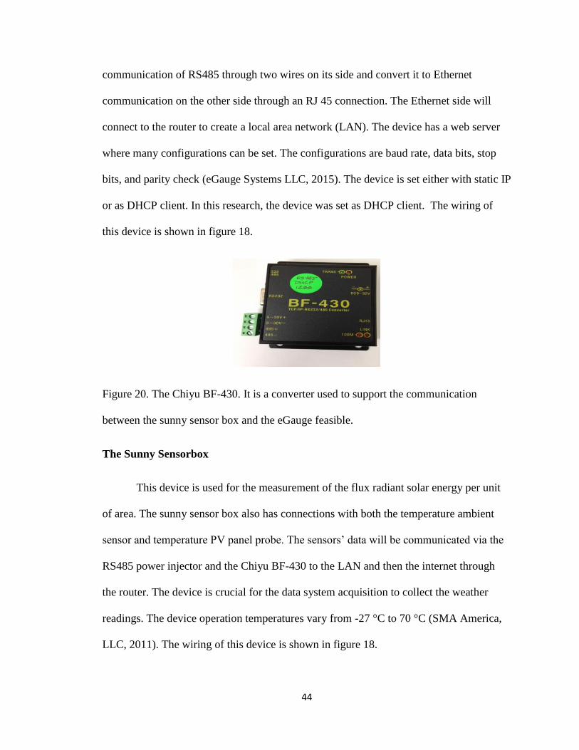
Figure 20. The Chiyu BF-430. It is a converter used to support the communication
between the sunny sensor box and the eGauge feasible.
The Sunny Sensorbox
This device is used for the measurement of the flux radiant solar energy per unit
of area. The sunny sensor box also has connections with both the temperature ambient
sensor and temperature PV panel probe. The sensors’ data will be communicated via the
RS485 power injector and the Chiyu BF-430 to the LAN and then the internet through
the router. The device is crucial for the data system acquisition to collect the weather
readings. The device operation temperatures vary from -27 °C to 70 °C (SMA America,
LLC, 2011). The wiring of this device is shown in figure 18.

45
Figure 21. The sunny sensor box. It is used to measure the irradiance and communicate
the temperature sensors signals to the eGauge via the Chiyu BF-430.
RS485 Power Injector
The RS485 Power injector works by merging and integrating the sunny sensor
box into the RS485 communication bus plus providing the sunny sensorbox with power
to operate. The RS485 power injector can supply up to five sunny sensor boxes (SMA
America, LLC, 2011). The wiring of this device is shown in figure 18.
Figure 22. The power injector. It is used in this research. The device supplies the sunny
sensor box with power.

46
Ambient Temperature Sensor
The ambient temperature is measured by TEMPSENSOR-AMBIENT which is a
sensor composed of a PT100 measuring resistor enclosed by plastic cage (SMA America,
LLC, 2011). The sensor will convey the data to the sunny sensor box then to the system.
This sensor can measure from -30 °C to 80 °C (SMA America, LLC, 2011). The wiring
of this device is shown in figure 18.
Figure 23. The ambient temperature sensor used in this research.
The PV Panel Surface Temperature Sensor
The temperature of the PV panel is measured using the PT100-NR. This sensor is
attached to the back of the panel to measure its temperature. The sensor is connected to
the sunny sensor box where the temperature is then sent to the system. The temperatures
that the sensor is capable of measuring vary from -20 °C to 110 °C (SMA solar
technology AG. 2009). The sensor is composed of a PT100 measurement resistor inside
plastic insulator. The wiring of this device is shown in figure 18.

47
Figure 24. The temperature sensor. It is used in this research to measure the PV panel
temperature. The sensor is attached to the back of the panel.
DC Current Transducers
These devices are used to measure the current generated by the PV panels. The
model used in this research is CR5220-20-12V. The positive wire coming from the PV
panel will go through the sensor to the load.The sensor will convey the equivalent of the
direct current to the eGauge via connections on the side of the sensor. The input range
varies from 0 to 20 amps. The DC current transducer is fed by 12 v DC (CRmagnetics
Inc., n.d.). The wiring of this device is shown in figure 18.
Figure 25. The DC current transducer. It was used in this research to measure the current
generated by the PV panels.
48
Router, Ethernet Cables, and Wires.
A router is connected to the system to link the multiple devices and the internet
providing a gateway. The router is set up as DHCP server to provide private IP addresses
to the LAN components. The IPs started from 192.168.0.100 to 192.168.0.199 with
network mask of 255.255.255.0. The router provides default gateway for the LAN which
is 192.168.0.1 with network mask of 255.255.255.0.
The wires used to connect the system were 10 American gauge wire (AWG) and 14
AWG. These gauges can bear the current coming from the panel. The Ethernet cable used
in this research is category five enhanced (CAT5E) which can carry information faster
with less interference between the lines than CAT5. The connectors used on the Ethernet
cable were registered jack 45 (RJ45) which has eight pins. The CAT5E Ethernet cable
attached to the RJ45 with the same order of colored lines to the pins on both sides of the
CAT5E cable forming the straight-through standard.

49
V. MECHANICAL SYSTEM
Background and Implementation
The mechanical system used in this research is a multi-task system. These tasks
include holding, securing, changing the tilt, and changing the direction of the PV panel.
The tilt and direction changing can be considered as a dual axis movement. The design
and implementation of this system was assigned by Dr. Asiabanpour to a group of
students as part of a tools design class. The group of students was comprised of Nicholas
Hawkes, Trevor Scott, Sean Syring, and Simona Curry. The product development process
(PDP) was used to design and implement this mechanical system. The System Modeling
and Renewable Technology (SMART) lab was considered as the customer for the
students. A rough implementation of the PDP steps was used, the steps included product
planning, concept development, system-level design, detail design, testing and
refinement, and production ramp-up (Ulrich & Eppinger, 2012). The key goals of the
mechanical system product are to help to conduct the experiment, to make it user
friendly, to produce it in the manufacturing lab, and to make multiple copies for other
users. The customer needs were identified and used to establish the mechanical system
specification, generate concepts and select concepts. The needs included the capability of
the system to hold and secure the PV panel, capable of rotating the PV panel, capable of
changing the tilt angle of the PV panel, ease of manufacture, ease of assembly, user
friendly, meet the target budget, and withstand fast wind. The previous needs were also
categorized into constraints (demands) and wishes. The two-axis movements were
considered as demands, the same classification was also applied to all the needs except
the user friendly, ease of manufacture and ease of assembly which were considered as

50
wishes. The second phase was to generate design concepts, then select one of them. The
specifications were identified based on the customer needs. Other steps in PDP were
implemented with system-level design then detail design. Drafts were generated for the
mechanical system parts using CAD. The mechanical system can achieve the rotation
movement by using castor and rotating base plates which have multiple holes in them to
secure the desired rotation angle by placing a bolt and nut in them. The tilting movement
mechanism was achieved by having two plates with holes and slit in them. These two
plates were shaped as the letter D. The parallel D-plates were attached to the SuperStruts
assembled to T-Slot Channel, which holds the PV panel. The D-plates were also attached
to the main vertical column through a bolt and nut. This center bolt is the pivot of rotation
for the main block that contains the PV panel and with this rotation the tilting movement
is achieved. Four sand blocks were also used on the four base square tubes that attached
to the rotating base plate. The final stages of the PDP were testing and refinement plus
production. The manufacturing labs in Texas State University were used to produce the
mechanical system. Many pieces of equipment and technologies where used including
waterjet machine, wilding, chop saw, and 3D printer.
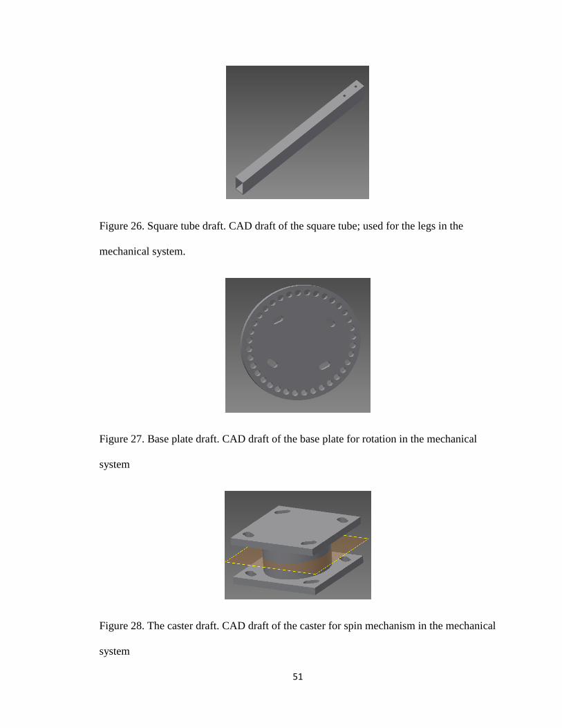
51
Figure 26. Square tube draft. CAD draft of the square tube; used for the legs in the
mechanical system.
Figure 27. Base plate draft. CAD draft of the base plate for rotation in the mechanical
system
Figure 28. The caster draft. CAD draft of the caster for spin mechanism in the mechanical
system

52
Figure 29. Fixed base plate. CAD draft of the fixed base plate in the mechanical
system.
Figure 30. Square tube adaptor plate. CAD draft of the square tube adaptor plate in the
mechanical system.
Figure 31. Square tube column. CAD draft square tube column in the mechanical system.

53
Figure 32. Sweeping mechanism pin. The CAD draft of the sweeping mechanism for D-
Plate in the mechanical system.
Figure 33. D-plate draft. CAD draft of the D-plate tilt mechanism in the mechanical
system.
Figure 34. T-slot bar .CAD draft of T-slot for tilt mechanism in the mechanical system.

54
Figure 35. The final assembly draft. The final assembly of the mechanical system
generated with Inventor Autodesk.
Figure 36. Parts draft and list. Parts draft and list generated by Inventor Autodesk.

55
Figure 37. Various parts draft and how to assemble.
Figure 38. Water jet machine used in the production.

56
Figure 39. 3D printer used in the production.
Figure 40. Chop saw used in the production.
Figure 41. SuperStruts. It is assembled to T-Slot Channel. This structure used to hold the
PV panel.

57
Figure 42. The rotating base plate used in the mechanical system.
Figure 43. The square tube adaptor base used in the mechanical system.
Figure 44. The square steel legs assembled to fixed base plate and caster.

58
Figure 45. The T-slot plastic bolt adaptor used in the mechanical system.
Figure 46. The D-plate with several tilt angle settings.
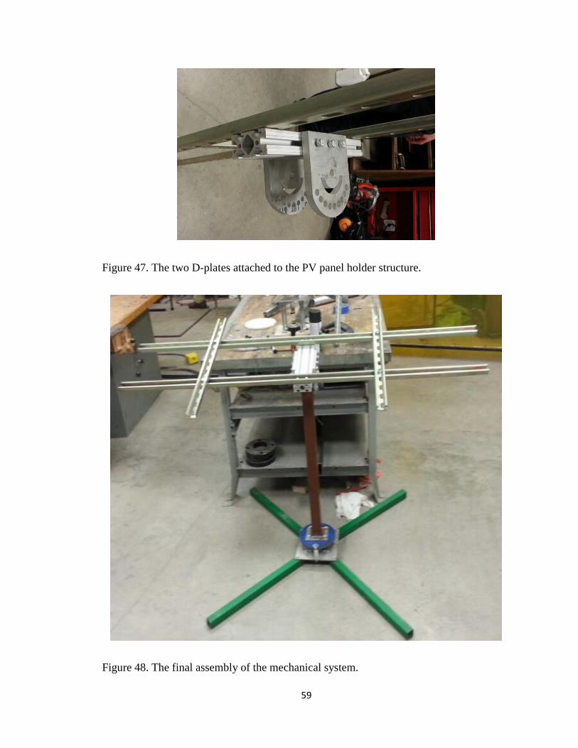
59
Figure 47. The two D-plates attached to the PV panel holder structure.
Figure 48. The final assembly of the mechanical system.

60
Finally the following table is shows the bill of materials (BOM) and the cost for
the mechanical system.
Table 6. Bill of materials.
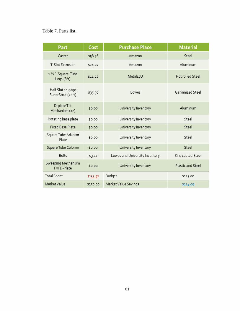
61
Table 7. Parts list.

62
VI. RESPONSE SURFACE METHODOLOGY
Introduction
The experiment was designed using Response Surface Methodology (RSM). The
selection of the method was based on both the objective of the experiment and the
number of factors and levels. RSM can be defined as a combination of mathematical and
statistical techniques effective for establishing, refining, and optimizing processes. It can
be also used for the design and creation of new products as well as improving current
ones (Myers & Montgomery, 2002). The RSM inputs are the identified independent
variables and the output will be the yield response which represents the performance
measure of the process. The unknown response can be approximated to a first, second or
third order model. The most used model is the second order model (Quadratic) especially
if curvature in the response is suspected. In this model main effects and interaction
between factors can be identified. In general, the second-order model is:
ji
jiij
k
j
jjj
k
j
jj xxxx 1
2
1
0
Where:
jx : Variable j
jjj ,,0 : Parameters of second-order model
: Model response
Variables ( jx ) usually are coded variables transformed from natural variables. The
independent variables are called natural variables when they are expressed with natural

63
units. “…Natural Variables can be transformed to coded variables which are
dimensionless with mean zero and the same spread or standard deviation” (Myers &
Montgomery, 2002, p.3).
An experiment, as described by Montgomery (1997), is a test or sequence of tests
where deliberate adjustments are made to the input variables of a system so that we may
detect and distinguish the causes for the changes in the output response. Designed
experiments are used in many disciplines and their impacts can be seen in almost every
aspect of our lives. They help to build our knowledge about certain processes and
systems which give us insight to enhance and improve performance. Engineering fields
are one of the biggest venues where design of experiment is used. Lower costs, new
ideas, new processes, new products, and new systems are invented due to the practice of
design of experiments.
Factors Identification
The first stage of the Response Surface Methodology is to identify the important
factors and their levels. They should have significant impact on the yield response. In this
experiment independent variables with multi levels are identified with a goal to study
their effect on the response yield and to find the optimum setting of the factors’ levels. A
model of typical process is applied with input, independent variables, uncontrollable
factors, and output. The photovoltaic effect is considered as the process. Two PV panels
are used as the input materials. The irradiance is considered another input to the process.
The date, time, and location were also considered as inputs to the process. The
temperature of the PV panels and the ambient temperature, though measured, were
considered as uncontrollable factors. General weather conditions were considered as

64
uncontrollable factors including the clouds and humidity. Tilt angle, azimuth angle, wind
intensity, and solar panel cleanness were considered as the controllable factors.
Figure 49. General model of a process or system. Adapted from “Design and analysis of
experiments” by D. Montgomery, (1997) p. 2
Input Output
Uncontrollable factors
Controllable factors
Process

65
Figure 50. The process diagram of the experiment.
Factor Levels in Feasible Ranges
For four independent variables three levels in the feasible ranges were identified:
A-tilt angle with three levels of 0º, 30º, and 60º from the horizon; B- azimuth angle with
three levels of 0º, 45º, and -45º from the south; C- the wind with three levels of 0, 5.5,
and 10 Km/h. The wind factor has been achieved through the use of a fan with multiple
speeds. The speed of the fan was measured through the use of a wind sensor. The fan was
placed in front of the panel with two feet distance from the center of the PV panel. The
fan was set to oscillate to make the air waves cover the entire PV panel. Finally, D- the
cleanness of the PV panels with three levels. Talc was used to emulate the cleanness of
Power
difference
Location
Photovoltaic
effect
Irradiance
Time
Panel’s temperature Ambient temperature
Weather conditions
Tilt angle Azimuth angle Wind Cleanness

66
the PV panels. Three levels of cleanness were determined based on the amount of the talc
scattered randomly on the surface of the PV panel. The levels were absence of talc as 0
gram, ten shakes of talc which equal 20 grams as second level, and the third level of
cleanness was twenty shakes of talc which is equal to 40 grams.
The two PV panels used in the experiment were identical. One panel was placed
on the dual axis mechanical system while the other was flat on the ground. The rheostats
loads that were used in the electrical system were identical. To overcome the minor
discrepancy of the initial output power of the two PV panels, a small calibration was
applied to them with R1=7.1Ω and R2= 7.4Ω. The irradiance of the flat PV panel was
determined as the input of the process and it was measured through the use of an
irradiance sensor placed flat beside the flat PV panel. Another irradiance sensor was
attached to the mechanical system and it was subjected to only two factors which were
tilt and azimuth angles (orientation of the PV panel), and their three levels. The second
sensor was recording the irradiance changes due to the changes in the tilt angles and the
azimuth angles. The yield response of the process was determined to be the recorded
power differences between the two PV panels. The selection of the power difference as
an output was to minimize the effect of the variation of the irradiance during the
experiment on the process. The four factors were selected with high, mid, and low levels.

67
Table 8. The four uncoded factors with their three levels.
level A=Tilt
Angle
(degree from
horizon)
B=Azimuth angle
(degree from
south)
C=wind
(Km/h)
D=Panel Cleanness
(grams of talc)
Low 0 -45 0 0
Mid 30 0 5.5 20
High 60 45 10 40
Table 9. The four coded factors with their three levels.
level A B C D
Low -1 -1 -1 -1
Mid 0 0 0 0
High 1 1 1 1

68
Design of Experiments
Experimental design has been implemented to characterize the process in terms of
how input parameters affect the power output. The main two kinds of designs of
Response Surface are Central Composite designs and Box-Behnken designs. The
selection of the type of Response Surface design is the second stage. In this experiment
Box- Behnken was used. The advantages of using Box-Behnken designs are a) to have
less design points than Central Composite designs which will make it less costly, and b)
high efficiency to estimate the first and second order model coefficients. The
disadvantages are the incapability to use runs from factorial experiments, the limitation of
three levels per factor while the Central Composite can have up to five, and finally they
cannot have runs with the extreme value of the factors ("What Is A Response Surface
Design? – Minitab, n.d.").
The software used for the design of experiment and to analyze the result is
Minitab. The setting included the selection of three replications and randomization to
reduce the bias. The software generated the following 81 uncoded runs.
Figurer 51. Minitab. Using Minitab Graphic user interface (GUI) to create RSM design of
experiment.

69
Figure 52. Using Minitab to create Box-Bhenken design of RSM.
Figure 53. Using Minitab GUI to select unblocked Box-Bhenken runs.
Figure 54. Using Minitab GUI to identify the high and low levels for each factor.
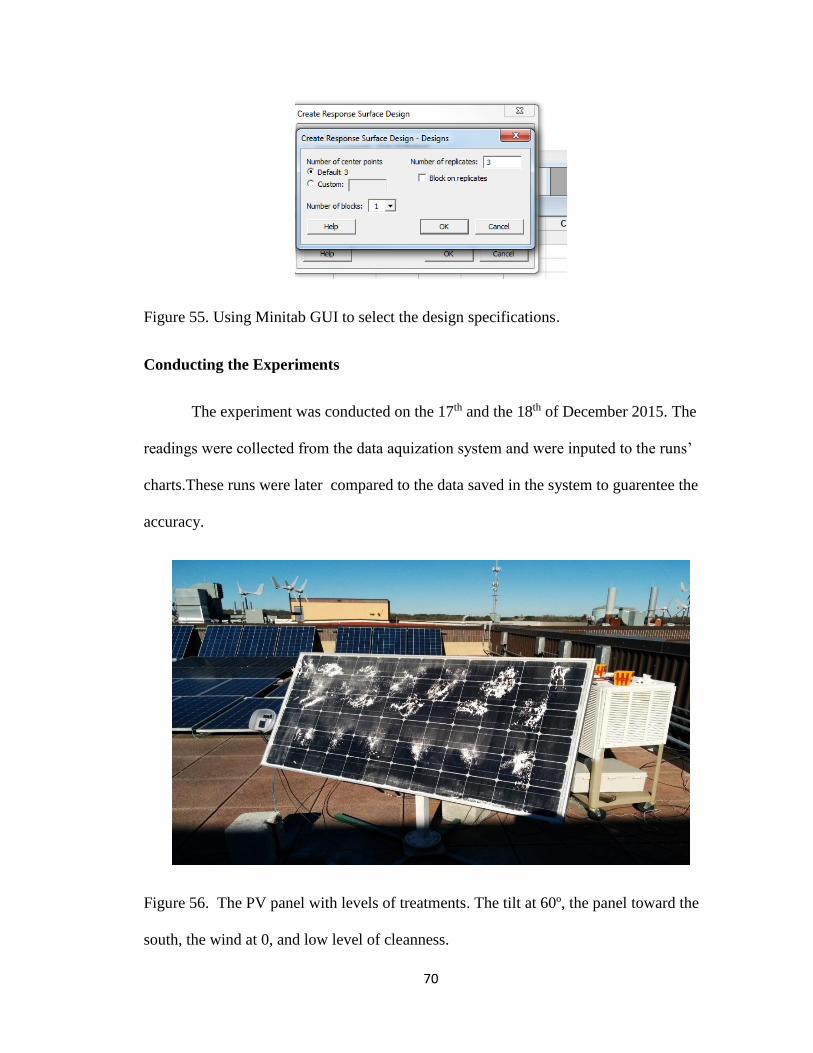
70
Figure 55. Using Minitab GUI to select the design specifications.
Conducting the Experiments
The experiment was conducted on the 17th and the 18th of December 2015. The
readings were collected from the data aquization system and were inputed to the runs’
charts.These runs were later compared to the data saved in the system to guarentee the
accuracy.
Figure 56. The PV panel with levels of treatments. The tilt at 60º, the panel toward the
south, the wind at 0, and low level of cleanness.

71
Figure 57. The PV panel subjected to the treatment during the experiment. The tilt at 0º,
the panel toward the east, the wind at 0, and mid-level of cleanness.
Appendixes B, C, and D show the runs, data, and some efficiency calculations.
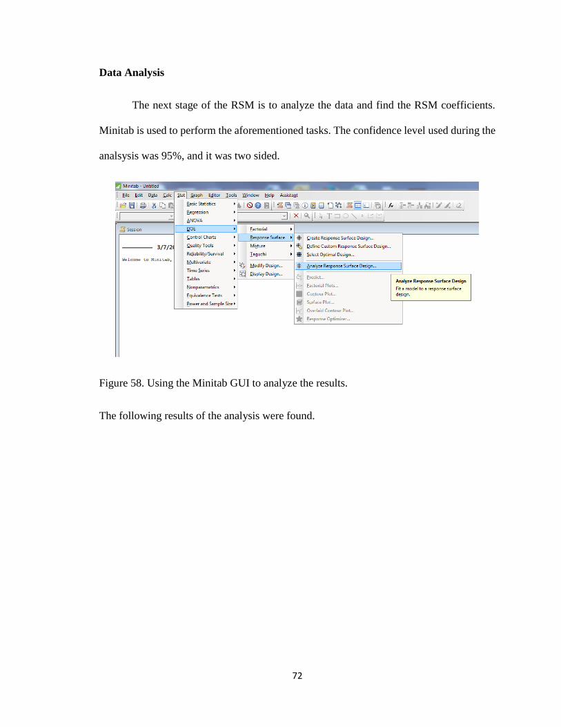
72
Data Analysis
The next stage of the RSM is to analyze the data and find the RSM coefficients.
Minitab is used to perform the aforementioned tasks. The confidence level used during the
analsysis was 95%, and it was two sided.
Figure 58. Using the Minitab GUI to analyze the results.
The following results of the analysis were found.

73
Table 10. The analysis of the data using Minitab.
Response Surface Regression: Power Difference versus A, B, C, D
Analysis of Variance
Source DF Adj SS Adj MS F-Value P-Value
Model 14 117742 8410.2 16.19 0.000
Linear 4 102326 25581.4 49.24 0.000
A 1 45412 45411.6 87.42 0.000
B 1 2604 2604.4 5.01 0.029
C 1 91 90.6 0.17 0.678
D 1 54219 54219.1 104.37 0.000
Square 4 9361 2340.2 4.50 0.003
A*A 1 2188 2188.2 4.21 0.044
B*B 1 2071 2071.3 3.99 0.050
C*C 1 254 253.7 0.49 0.487
D*D 1 2327 2327.0 4.48 0.038
2-Way Interaction 6 6056 1009.3 1.94 0.087
A*B 1 2033 2033.2 3.91 0.052
A*C 1 377 377.4 0.73 0.397
A*D 1 161 160.6 0.31 0.580
B*C 1 2617 2616.7 5.04 0.028
B*D 1 4 4.1 0.01 0.930
C*D 1 864 863.6 1.66 0.202
Error 66 34286 519.5
Lack-of-Fit 10 7254 725.4 1.50 0.163
Pure Error 56 27032 482.7
Total 80 152028
Model Summary S R-sq R-sq(adj) R-sq(pred)
22.7920 77.45% 72.66% 66.19% Coded Coefficients
Term Effect Coef SE Coef T-Value P-Value VIF
Constant 23.78 7.60 3.13 0.003
A 71.03 35.52 3.80 9.35 0.000 1.00
B 17.01 8.51 3.80 2.24 0.029 1.00
C 3.17 1.59 3.80 0.42 0.678 1.00
D -77.62 -38.81 3.80 -10.22 0.000 1.00
A*A -23.39 -11.69 5.70 -2.05 0.044 1.25
B*B -22.76 -11.38 5.70 -2.00 0.050 1.25
C*C -7.96 -3.98 5.70 -0.70 0.487 1.25
D*D 24.12 12.06 5.70 2.12 0.038 1.25
A*B 26.03 13.02 6.58 1.98 0.052 1.00
A*C -11.22 -5.61 6.58 -0.85 0.397 1.00
A*D -7.32 -3.66 6.58 -0.56 0.580 1.00
B*C -29.53 -14.77 6.58 -2.24 0.028 1.00
B*D -1.17 -0.58 6.58 -0.09 0.930 1.00
C*D -16.97 -8.48 6.58 -1.29 0.202 1.00
Fits and Diagnostics for Unusual Observations
Power
Obs Difference Fit Resid Std Resid
4 88.40 39.60 48.80 2.39 R
21 46.00 102.13 -56.13 -2.74 R
54 76.70 23.78 52.92 2.46 R
66 2.00 60.59 -58.59 -2.86 R
R Large residual

74
Figure 59. Four-in-one residual plot generated by Minitab.
The normal probability plot on the top left of figure 59 shows normal distribution
of the residuals. The histogram plot in the same figure shows the frequency of the
residual. The highest residual frequency is around zero. Unusual high residuals (-60) can
be seen with low frequency. The residual versus fits plot shows no pattern which
supports the regression model. The residual versus observation order shows
randomization which supports the independence assumption.

75
Figure 60. The main effect plot generated using Minitab for the yield response.
The main effect plot for the response indicates that the 60 º angle of tilt produces
the highest output, while the zero degree gives the lowest for this season of the year. The
same plot shows zero degree azmuth angle (orientation of the PV panel) gives the highest
response while -45º gives the lowest. The response yielded to 45 º is close to the zero
degree of the azmuth angle for this season. The same plot shows almost the same
response for the three levels of treatment of the wind. Finally the clean panel with no talc
gives the highest yield response. The response is decreasing with the increment of the talc
on the subjected panel.

76
Figure 61. The surface plot of the yield response as generated using Minitab.
Figure 62. The interaction plot. The interaction plot for the yield response with the four
factors and their three levels as generated using Minitab.
A 30B 0
C 1
D 1
Hold Values
05-
0
00
52 5
0
50
0
-5050
500ecnereffiD
B
A
20-
002
025 5
0
0
2
1
005
020400
ecnereffiD
C
A
-50
0
50
00
25 5
0 1
050
2
1
2
50
001
ecnereffiD
D
A
2
02- 1
0
20
-500 0
50
200ecnereffiD
C
B
0
30
06
-5-500
0
0
0
1
050
2
1
2
06
09
ecnereffiD r
D
B
0
25
05
01
0
5
0
1
02
2
1
2
05
75
0
5
ecnereffiD r
D
C
ecnereffiD rewoP fo stolP ecafruS

77
Figure 63. Contour plot of the yield response. The plot shows the levels of two factors at
a time with corresponding response.
The yield response equation calculated by Mintab through Regression.
The Regression Equation in Uncoded Units is
𝑃𝑜𝑤𝑒𝑟 𝐷𝑖𝑓𝑓𝑒𝑟𝑒𝑛𝑐𝑒 = 4.1 + 2.272 𝐴 + 0.241 𝐵 + 23.6 𝐶 − 50.8 𝐷 − 0.01299 𝐴2
− 0.00562 𝐵2 − 3.98 𝐶2 + 12.06 𝐷2 + 0.00964 𝐴𝐵 − 0.187 𝐴𝐶− 0.122 𝐴𝐷 − 0.328𝐵𝐶 − 0.013𝐵𝐷 − 8.48 𝐶𝐷
The Regression Equation in coded Units is
𝑃𝑜𝑤𝑒𝑟 𝐷𝑖𝑓𝑓𝑒𝑟𝑒𝑛𝑐𝑒 = 23.78 + 35.52 𝐴 + 8.51 𝐵 + 1.59 𝐶 − 38.81 𝐷 − 11.69 𝐴2 −11.38 𝐵 2 − 3.98 𝐶2 + 12.06 𝐷2 + 13.02 𝐴𝐵 − 5.61 𝐴𝐶 − 3.66 𝐴𝐷 − 14.77 𝐵𝐶 −0.58𝐵𝐷 − 8.48 𝐶𝐷
A 30B 0
C 1
D 1
Hold Values
B*A
50250
40
20
0
-20
-40
C*A
50250
2.0
1 .5
1 .0
0.5
0.0
D*A
50250
2.0
1 .5
1 .0
0.5
0.0
C*B
400-40
2.0
1 .5
1 .0
0.5
0.0
D*B
400-40
2.0
1 .5
1 .0
0.5
0.0
D*C
210
2.0
1 .5
1 .0
0.5
0.0
>
–
– –
–
< -30
-30 0
0 3030 60
60 90
90
Difference
Power
Contour Plots of Power Difference

78
The calculated P-values through the ANOVA indicate the significance of the
factors and their interactions on the yield response. Some of the factors have a high P-
value and they were removed from the edited equation (higher than 0.05). These factors
or their interactions are: C, C², AC, AD, BD, and CD. Some of the second order
parameters have a critical P-value and are kept in the final equation. These include BB
and AB with a P-value equal to 0.05 and 0.052 respectively. The wind factor and its
interactions showed insignificant impact on the response except the interaction with the
azimuth angle (orientation) of the PV panel. This might be due to uncontrollable natural
wind occurring during the experiment.
The final equations are
Regression Equation in Uncoded Units.
𝑃𝑜𝑤𝑒𝑟 𝐷𝑖𝑓𝑓𝑒𝑟𝑒𝑛𝑐𝑒 = 4.1 + 2.272 𝐴 + 0.241 𝐵 − 50.8 𝐷 − 0.01299 𝐴2 − 0.00562 𝐵2
+ 12.06 𝐷2 + 0.00964 𝐴𝐵 − 0.328𝐵𝐶
Regression Equation in Coded Units.
𝑃𝑜𝑤𝑒𝑟 𝐷𝑖𝑓𝑓𝑒𝑟𝑒𝑛𝑐𝑒 = 23.78 + 35.52 𝐴 + 8.51 𝐵 − 38.81 𝐷 − 11.69 𝐴2 −11.38 𝐵 2 + 12.06 𝐷2 + 13.02 𝐴𝐵 − 14.77 𝐵𝐶
Optimization
The opimization of the response was determined through the use of Mintab. The
software generated the optimum settings of the factors to maximize the yield response.
The following table and figure show the Minitab-generated optimum results.

79
Table 11. Minitab optimization results.
Response Optimization: Power Difference Parameters
Response Goal Lower Target Upper Weight Importance
Power Difference Maximum -59.2 110.8 1 1
Starting Values
Variable Setting
A 0
B 0
C 0
D 0
Solution
Power
Difference Composite
Solution A B C D Fit Desirability
1 60 45 0 0 119.178 1
Multiple Response Prediction
Variable Setting
A 60
B 45
C 0
D 0
Response Fit SE Fit 95% CI 95% PI
Power Difference 119.2 20.1 (79.0, 159.3) (58.5, 179.9)
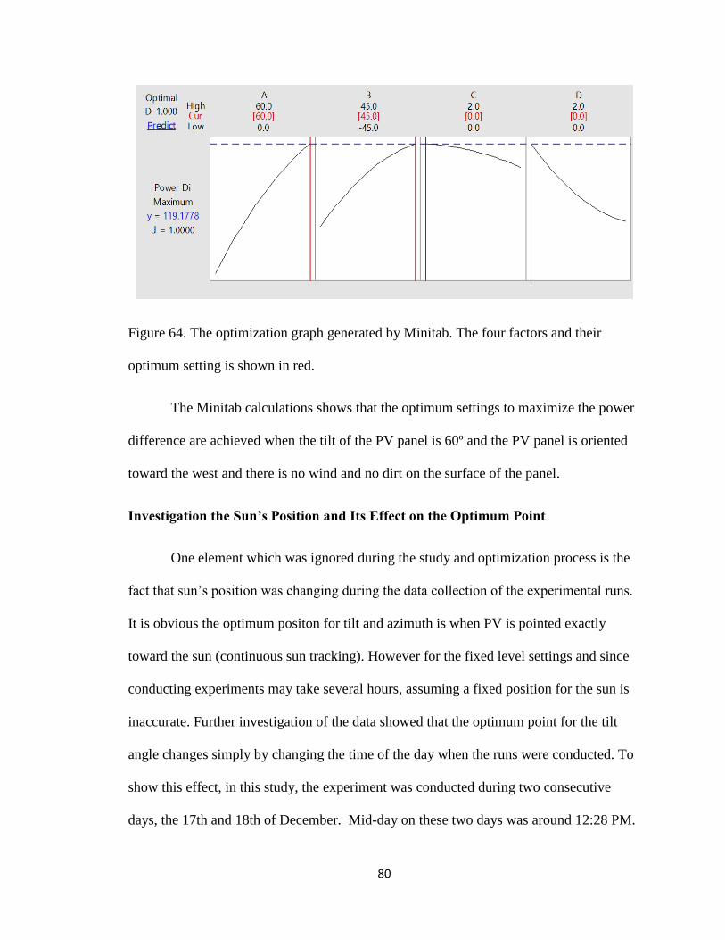
80
Figure 64. The optimization graph generated by Minitab. The four factors and their
optimum setting is shown in red.
The Minitab calculations shows that the optimum settings to maximize the power
difference are achieved when the tilt of the PV panel is 60º and the PV panel is oriented
toward the west and there is no wind and no dirt on the surface of the panel.
Investigation the Sun’s Position and Its Effect on the Optimum Point
One element which was ignored during the study and optimization process is the
fact that sun’s position was changing during the data collection of the experimental runs.
It is obvious the optimum positon for tilt and azimuth is when PV is pointed exactly
toward the sun (continuous sun tracking). However for the fixed level settings and since
conducting experiments may take several hours, assuming a fixed position for the sun is
inaccurate. Further investigation of the data showed that the optimum point for the tilt
angle changes simply by changing the time of the day when the runs were conducted. To
show this effect, in this study, the experiment was conducted during two consecutive
days, the 17th and 18th of December. Mid-day on these two days was around 12:28 PM.
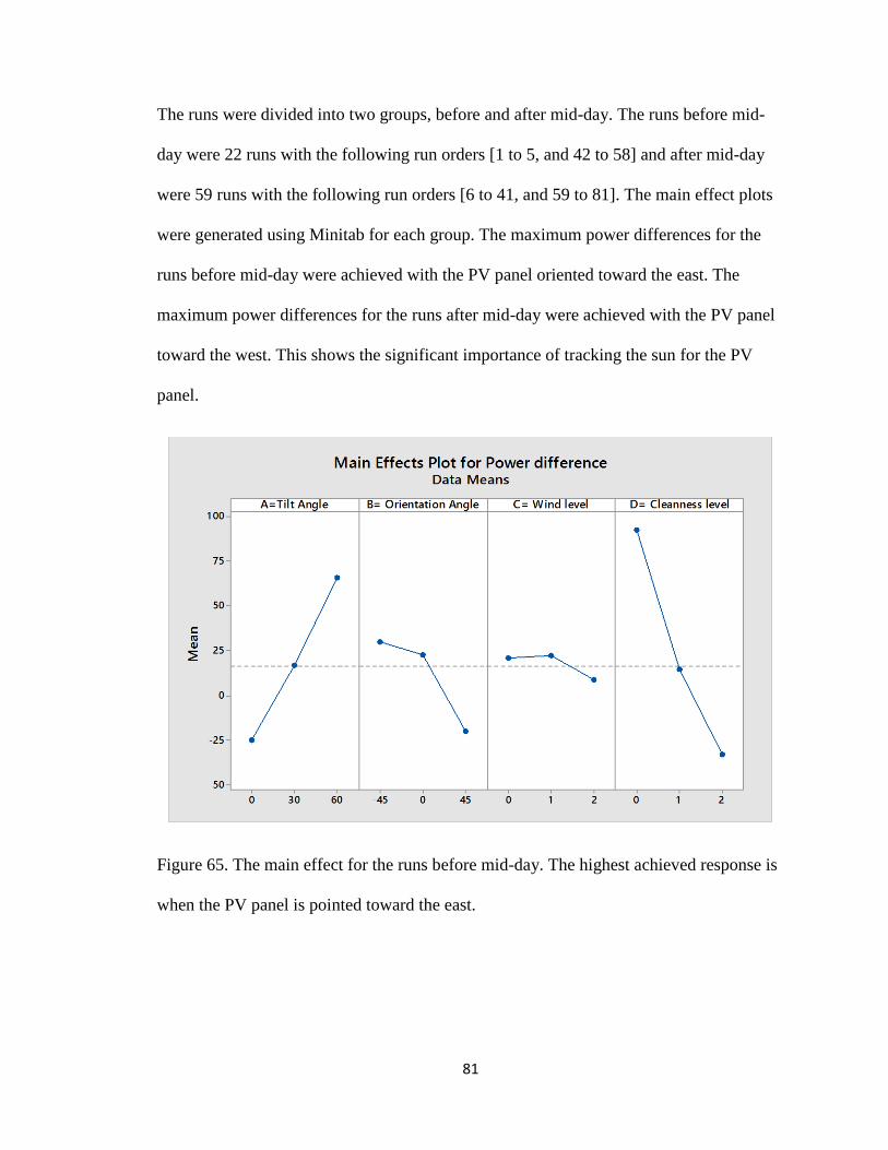
81
The runs were divided into two groups, before and after mid-day. The runs before mid-
day were 22 runs with the following run orders [1 to 5, and 42 to 58] and after mid-day
were 59 runs with the following run orders [6 to 41, and 59 to 81]. The main effect plots
were generated using Minitab for each group. The maximum power differences for the
runs before mid-day were achieved with the PV panel oriented toward the east. The
maximum power differences for the runs after mid-day were achieved with the PV panel
toward the west. This shows the significant importance of tracking the sun for the PV
panel.
Figure 65. The main effect for the runs before mid-day. The highest achieved response is
when the PV panel is pointed toward the east.

82
Figure 66. The main effect plot for the runs in the afternoon. The highest achieved
response is when the PV panel is pointed toward the west.
Efficiency Calculations
The efficiency of both PV panels were calculated. The efficiency equation is
100
AP
AP
in
out
Where:
P is power and A is the area of the PV panel.
𝐴 = 1.11502347 𝑚2.

83
The first PV panel was the panel which was subjected to the manipulations. The
efficiencies of this PV panel were calculated for all runs once with irradiance1 as input
and later with irradiance2. The second PV panel is the flat panel. The efficiencies
calculations were done with the irradiance2 as the input. The irradiance gains are also
calculated for all runs.
Irradiance gain = Irradiance 1- Irradiance 2
The flat PV panel efficiency was relatively constant, while the first PV panel efficiency
was affected with the treatment levels.
Figure 67. The received irradiance for the two PV panels.
0
200
400
600
800
1000
1200
1 4 7 10 13 16 19 22 25 28 31 34 37 40 43 46 49 52 55 58 61 64 67 70 73 76 79
Irradiance 1 Irradiance 2

84
Figure 68. The various recorded efficiency of the two PV panels during the experiment.
Appendix D shows the calculated efficiency for all the runs.
Validation
The PV panel was subjected to the founded optimum levels of treatments on the
26th of February. A sample of the data was collected from the 27th record.
Table 12. Validation sample of data. A sample of data from the 27th of February 2016
with the optimum settings of 60º, 45 º from the south, 0 wind and 0 talc.
Date and
time
Power1 Power2 Power
difference
Irrediance1 Irrediance2
2/27/2016
15:45 PM
169.8W
60.5W
109.31W
1000.8W
394.25W

85
VII. CONCLUSIONS AND FUTURE WORKS
Conclusions
The four factors investigated in this research to optimize the performance of the
PV panels have various impacts on the power output. In addition to these factors, other
variables such as the date/time and the location of the PV panels affect the performance
of the PV panels as well. To minimize the impact of the variation of the irradiance during
the day, due to uncontrollable factors such as clouds and general weather conditions, this
research considered the difference between the power generated by the adjustable panel
(subjected to the factors) and the control panel (i.e., flat panel) as the optimization
objective. An adjustable mechanical system was designed and developed for this
research. Additionally, electrical and data acquisition systems were developed for this
purpose as well. The research used design of experiments and response surface
methodology to plan, analyze, and optimize the experiments. Minitab software was used
to achieve these purposes. The final findings showed the influencing factors on the yield
response. The tilt, azimuth angle (orientation), and cleanness were effective factors while
wind’s impact within the tested range was insignificant. The optimum findings were: 60º
tilt from the horizon, 45º from the south, and panel in clean condition resulted in the
maximum response (i.e., power difference between subject and control panels).

86
Future Works
Much research can be done on PV panel performance and efficiency. Such
research may include the following:
Developing automated cleaning systems to overcome the accumulated dust
problem.
Developing smart PV panels with the capability of self-cleaning and/or self-
cooling to enhance the performance.
Developing a self-monitoring PV panel to collect the performance data.
Enhancing the efficiency of the PV panels through studying different materials,
technologies, manufacturing processes, filtering, geometry, and ads-on (e.g., built
in cooling system, etc.).
Studying the environmental effects (e.g., wind, rain, cloud, dust, humidity) on the
performance of different PV panels’ technologies (e.g., silicon monocrystalline,
silicon polycrystalline, perovskite, etc.).
Studying and developing optimum settings (tilt and orientation) for the PV panels
for each month or permanently in designated locations.
Studying the irradiance pattern for designated locations.
Studying the degradation rates of PV panels at designated locations for different
technologies.
Studying the effect of the local weather conditions on the degradation rates.
Studying the effect of pollution on both the performance and degradation rates for
various PV panels’ technologies.

87
Collecting and recording detailed data of the PV panel performance in designated
locations throughout the year.
Creating a database for the performance of the PV panels in Texas through the
cooperation with regional partners.
Creating a cost effective, passive sun tracking system with no electrical
consumption.
Creating a cost effective, active sun tracking system with low power
consumption.
Creating a remotely-controllable, through the internet, sun tracking system for
distant locations.

88
APPENDIX SECTION
APPENDIX A. THE EGAUAGE SOFTWARE AND CAPABILITIES
This appendix is entirely cited and adapted from the eGauge website ("help",
2016) to describe the device settings and functions.
eGauge gathers data and can convey them to a spreadsheet programs like excel,
Open office calc, or gnumeric. A friendly graphic user interface (GUI) will help to
achieve that. The kind of data, time-range, and resolution of the conveyed data can be
selected through this GUI. The data to be exported as a csv file can be the average values
during successive time or cumulative values. Kilowatts (kW) will be the unit for the
energy if exported as average values, while the unit will be kilowatt-hours (kWh) if
exported as cumulative values. The time range can be specified by the user with the
selection of the beginning and the ending of the time period. Another important feature
eGauge provides is the time interval between data points; the default is one data point
exported per day (which can be changed by the user for one data point exported per hour,
minute, or second). These exported data are arranged from the newest to the oldest. To
plot them the user needs to invert the time order to make the advancement of time from
left to right. Such inversion can easily be done by the spreadsheet programs by using the
sort function for the exported data before plotting them.
The general settings of the eGauge include: the date and time, the geographic
location, the geographic region, the minimum interval for public usage data, the proxy-
server hostname, and data sharing. The date and time is when record-keeping is initiated,
overlooking any data chronicles before it without losing them, and later the user can

89
easily shift this point of time toward any direction if needed. The software gives another
helpful option for the record starting point. By putting “now” as the starting date and
time, the user establishes that moment as the starting point, automatically ignoring earlier
data. The geographic location setting will identify the geographic location of the eGauge
with a small modification to ensure the exact location will not be exposed. It includes the
latitude and longitude of the site with a positive value for northern latitudes and a
negative for southern latitudes, and in the same manner, a positive value will be issued to
the eastern longitudes while a negative to the western longitudes. Another feature is the
map, which will provide a separate window to show the map of the entered location. The
geographic region shows where the eGauge is installed and guarantees regulatory
compliance by controlling the frequency bands used if a home plug av interface is used.
The minimum interval for public usage data setting is used to make a limitation on the
data available for public users by controlling its resolution. The default of the data
resolution is one minute and it can be changed to many other options that can reduce the
resolution to boost security. The local and licensed users will have full-resolution data.
The proxy-server hostname setting will indicate the hostname (or IP address) of the
machine that is running the proxy-server. The proxy-server makes it feasible to connect
to eGauge at URI http://name.egaug.es. Data Sharing will control the sharing of the
collected data, which can be disabled or enabled, with a service provider. This sharing
can also be customized to advance the collected data to a URI (unless an empty string is
placed instead of it) with a particular push option and specific push interval that will
define the time interval between consecutive data pushes. There are various push options
and they can be used to indicate what or how data are being pushed, including calculate

90
totals and virtual registers, push the data with second by second granularity, compress the
push data, and secure connections that demand the server has an authentication which can
be confirmed as legitimate. All the above push options are separated by commas when
they are listed together.
The network settings include: the hostname setting, the automatically obtain
address with dynamic host configuration protocol (DHCP) setting, the IP address setting,
the netmask setting, the network setting, the broadcast address setting, the gateway
address setting, the name server setting, and the enable bridging setting. The hostname is
a setting that will define the hostname of the eGauge, changing this name without
informing the server http://egauge.es/ will result in losing the connectivity with it.
“Automatically obtain address with DHCP” is the setting that will determine whether the
eGauge will manually be set with network configuration or it will do that automatically
via the DHCP. If the latter option is selected then the rest of the network setting will be
grayed out. The IP address setting will statically assign the eGauge an IP address (e.g.,
192.168.0.99). The netmask setting will assign the IP mask address for the eGauge (e.g.,
255.255.255.0).The network setting will illustrate the network IP address used by the
eGauge (eg.192.168.0.0). The broadcast address setting will assign the IP broadcast
address used by the eGauge (e.g., 192.168.0.255). The gateway address setting will
assign the IP address of the gateway used by the eGauge (e.g., 192,168.0.1). The name
server setting 1-4 will specify the IP address of the domain name system (DNS) servers
which used by the eGauge. The DNS servers are used to resolve the domain-names. The
eGauge typically uses a single network interface to communicate, such as a homeplug or
hardware Ethernet. If we have both interfaces and the enable bridging setting is on, the

91
interfaces will be bridged together. The eGauge in this case will forward all the traffic
between them, forming one logical network. This scenario is helpful when numerous
eGauges are installed at one site, hardwiring one egauge and the second one can connect
to it using the homeplug, all the devices will be joined in the LAN. Spanning tree
protocol (STP as defined by IEEE 802.1D) in this mode are enabled to detect and
prevent the looping resulting from the redundancy which might over flood the LAN with
the same looped packets. The manufacturer advises to design the connections carefully
with no loops or use equipment that back STP.
Building automation control network (BACnet) protocol, the eGauge software
contains many settings for this protocol: enable BACnet support setting, protocol to use
for BACnet data link setting, BACnet device id unique to this device setting, and energy
unit setting. The first setting is to enable its support which the manufacturer does not
recommend selecting if the user has no knowledge of this protocol. The second setting is
for the protocol to use for BACnet datalink, eGauge can communicate BACnet either
through the Ethernet packets or over BACnet/IP (BIP). There are many other of datalink
for the BACnet like ARCNET, MS/TP over RS-485, Point-To-Point over RS-232, and
LonTalk, but the eGauge is not supporting them directly, encapsulating BACnet data
inside UDP/IP packets. In our experiment the selection for this option is Ethernet since
this what we use for the datalink. The third setting is for BACnet device id unique to this
device, as each BACnet-capable device needs to have a unique device instance number,
which can be any number between 0 and 4,194,303. And finally the energy unit setting,
where the unit used for the cumulative value of energy registers will be set by this
setting. The default is watt-second (Ws), while the alternative is kilowatt-hours (kWh).

92
Another feature the eGauge software provides is an alert service. This can be done
through the alert settings and select how the eGauge will dispatch many alerts through
short message service (sms) to a phone, email, or both. The recipients of such alerts can
be up to four. Those alerts can be prioritized with the settings. The alerts have a delay of
30 seconds. The alerts are divided into two kinds, system defined and user defined. The
first one can dispatch circumstances like a change in the eGauge configuration occurred
or a connection to a remote device has been formed. User defined alerts on the other hand
can be provoked by events defined by the user like a drop in solar production below a
certain value.
The software of the eGauge can specify how the alert is conveyed to the desired
recipient by setting the email Gateway with the hostname of mail server. The eGauge will
try to send the email straightly to the destination address. The same thing can be said
about the SMS which will be send to sms-gateway, yet if a firewall has been set to
prevent this direct connection, the eGauge settings can include hostname of a mail server
who will forward the email to the desired destination. This server can be on the same
LAN, Which will take the email without authentication, or a mail server on the internet
that the eGauge user has a valid account on, through the settings the username and
password will be provided and then the device will use that mail server. in another word
the eGauge tries to send the messages by using simple mail transfer protocol (SMTP) to
the mail exchange hosts articulated by Mail exchange records (MX-records) for a given
domain. If no MX records happen, then the eGauge will try to send the message to the
server linked to the domain name. The setting that includes a hostname will make the
eGauge convey all mail through this host. Filling the part of username for mail server in

93
the settings makes the eGauge convey the mail with transport layer security (TLS)
encryption and the authentication through port 587 of the host, authenticating itself with
the specified username and password. If no username is provided in the settings the
delivery will be in plain text through port 25.
Alert Destinations
It can be set to four recipients with messages of different level of priorities.
Message Format
The message format is an option to choose whether to send all the pending alerts
with one email (by selecting Email), the other option will send only the most recent alerts
with highest priority, keeping the message size below 140 characters (by selecting short
Email). The format also includes selecting mobile service provider to send the SMS
through it.
Email address or phone number
In this setting the email address will provided here and for SMS the phone number.
Minimum Alert Priority
This setting will determine the least priority number of an alert that can start
sending message to the alert destination.
System Alert Priorities
Although they are predefined, they can be controlled by selecting their priority
and which recipients they will deliver to. The priority is defined by assigning numbers
with 0 as the minimum (will not trigger sending to anyone) and 7 as the highest.

94
User-defined Patterns
It is comprised of many setting starting with the name of the user defined alert
patterns. The name will inform the recipient of the alert about the nature of the alert
condition. If this setting kept blank then no user defined will be use in the system. The
trigger condition is another setting, when they are satisfied they will initiate the alert to be
send. These conditions are consisting of three parts, left side, comparison operator, and
right side. There are many types of comparison operator used by the software, less than
(“<”), less or equal (“<=”), equal “=”), greater or equal (“>=”), or greater (>). They are
used to compare the right hand side to the left side and if the comparison is true then the
alert is will be initiated. Another important setting associated with this subject is the
frequency of the trigger conditions to be checked, which can be from one second to up to
one year. That been said the eGauge software do an evaluation all the alert condition
when the device is starting up, and the first minute of each hour (checking the hourly
conditions), The first hour of each day (checking the daily conditions), The first hour of
Sunday (checking the weekly conditions), the first hour of the first day of the month
(checking the monthly conditions), the first hour or the year (checking the yearly
conditions). The settings include the message to be send to the recipient which by default
shows the conditions with the right side, operator, and left side.
Access Control
This part of the software settings will allow the user to control who can access the
eGauge and how. It allows up to 15 users to be included and defined with exclusive
name, setting describes how the user may access, plus a password to secure the
authentication of the user identity. The software will have a default user under the name

95
of owner who can alter the setting of the device when connected through the Local Area
Network (LAN). That is both the user and the eGauge are having the same network name
address. A new user to be easily added through the access settings. The name of the user
can have letters, digits, or underscore character “_” but it can’t be administrator as this
name is reserved. Then that user can be assigned to special privileges through the settings
which include:
Viewing all the data plus altering the settings from anywhere.
View all the data and change the settings only from the LAN.
View all the data and the eGuage settings without the capability to change
the settings.
View limited data for a specific user.
The password for the access control settings is to be defined and set for each user,
the only downside of the software password for access control setting is when the user
changes the password, it will be sent via the internet to the device without any
encryption. This might carry the risk of having someone intercepting this information and
steal the password.
Date & Time
The settings of the date and time in the software include:
Time-server (NTP) hostname(s): This setting will provide the eGauge with an IP address
or hostname who will supply it with the current time. Network Time protocol (NTP) is
used to provide the time. Four servers in the north-america.pool.ntp.org domain are the
default to supply the time in the North American region. This is expressed by

96
{0..3}.north-america.pool.ntp.org The software can have up to eight server-names which
can be done by the brace expansion. The time zone is another setting that we can add and
select the one that match our location.

97
APPENDIX B. THE EXPERIMNT’S RUNS. THE EXPERIMNT’S RUNS AS
GENERATED BY MINITAB SOFTWARE.
StdOrder A=Tilt Angle B= Orientation Angle C= Wind level D= Cleanness level
1 30 -45 1 0
2 0 -45 1 1
3 0 0 2 1
4 60 0 2 1
5 30 0 0 2
6 30 0 0 2
7 30 45 1 0
8 30 0 2 2
9 60 0 2 1
10 30 45 1 2
11 30 0 1 1
12 30 0 1 1
13 30 -45 2 1
14 60 45 1 1
15 0 0 0 1
16 0 45 1 1
17 60 0 1 2
18 0 0 1 2
19 30 0 0 0
20 0 0 0 1
21 60 0 1 0
22 60 0 2 1
23 30 45 0 1
24 30 -45 1 2
25 30 -45 0 1
26 30 -45 2 1
27 30 45 1 0
28 30 0 1 1
29 30 45 0 1
30 30 0 1 1
31 0 0 1 0
32 30 -45 1 2
33 0 -45 1 1
34 30 45 0 1
35 30 0 0 0
36 0 0 1 0
37 0 -45 1 1
38 30 45 1 2
39 60 45 1 1
40 60 0 1 2

98
StdOrder A=Tilt Angle B= Orientation Angle C= Wind level D= Cleanness level
41 30 -45 0 1
42 30 45 1 2
43 30 0 1 1
44 60 0 0 1
45 30 45 2 1
46 0 0 1 2
47 60 -45 1 1
48 30 -45 2 1
49 30 0 1 1
50 30 0 2 0
51 60 0 1 0
52 60 -45 1 1
53 0 45 1 1
54 30 0 1 1
55 0 0 2 1
56 30 0 2 2
57 0 0 2 1
58 30 45 2 1
59 30 -45 1 0
60 30 -45 1 2
61 30 45 2 1
62 0 0 1 0
63 30 0 2 0
64 30 0 0 2
65 60 0 1 2
66 30 0 0 0
67 0 0 0 1
68 0 0 1 2
69 60 0 0 1
70 60 0 0 1
71 60 0 1 0
72 30 0 2 2
73 30 -45 1 0
74 30 0 1 1
75 60 45 1 1
76 30 0 1 1
77 60 -45 1 1
78 0 45 1 1
79 30 0 2 0
80 30 45 1 0
81 30 -45 0 1

99
APPENDIX C. THE COLLECTED DATA. THE RUNS AND THE COLLECTED
DATA FOR VARIOUS VARIABLES.
Noise factors Irradiance Responses
StdOrder Panel 1
Temp
Panel
2
Temp
Amb.
Temp 1 2
Power
1
Power
2
Volt.
1
Volt.
2
Power
diff.
1 35.5 31.9 15.6 904 650 156 80.7 32 23.14 75.3
2 33 32 15.3 720 652 70.6 81.5 21.5 23.16 -10.9
3 30.3 31.5 15.8 888 655 67 82 21 23.2 -15
4 32.1 31.5 16.33 1064 656 170.4 82 33.3 23.2 88.4
5 35.8 32.4 16.3 1038 656 67.5 82 21.04 23 -14.5
6 37 32.8 16.3 1035 652 93.5 82 24.7 23.2 11.5
7 38 33 17.3 944 653 142 81 30.5 23.14 61
8 37.6 31.8 16.7 1070 650 77.5 81.1 22.5 23.08 -3.6
9 36 30.9 16.9 1052 647 97.5 79.4 25 22.86 18.1
10 35 32.5 17.5 1046 640 72 77 21.7 22.6 -5
11 32.5 29 18 996 631 73 75 21.8 22.25 -2
12 32.4 30 17.73 981 625 93 73 24.6 21.9 20
13 30.7 30.5 18.5 731 610 61.5 71.2 20.06 21.6 -9.7
14 31.5 30.9 18.5 990 601 100 68.8 25.5 21.3 31.2
15 32.5 28.9 19 598 600 40 68.3 16.2 21.3 -28.3
16 30 27.3 19 553 588 27.8 65.5 13.45 20.74 -37.7
17 30 27.3 19 1014 577 97 62.6 25.16 20.35 34.4
18 30.6 26.6 19.2 563 558 23.5 59.9 12.4 19.89 -36.4
19 32 28 19.8 924 554 158 58 32 19.6 100
20 33.4 27.8 19.2 529 547 24.6 58 12.86 19.5 -33.4
21 33 27 19.2 964 521 98 52 25.2 18.5 46
22 33 29.5 20 981 533 103 54.7 25.9 19 48.3
23 34.6 26 20 906 512 83 50.3 23.29 18.21 32.7
24 31.6 26.4 20 539 500 25 48.5 12.9 17.9 -23.5
25 29.4 27 20.4 520 488 33.4 47 14.7 17.6 -13.6
26 29.1 26 20.4 514 484 28 45 13.47 17.3 -17
27 30 26.3 20.4 888 467 137 43.9 29.8 16.97 93.1
28 31.43 25.9 20.1 834 459 80 41.5 22.8 16.53 38.5
29 33.3 26.5 21 873 451 83.5 40.9 23.3 16.39 42.6
30 33.8 26.3 20.5 811 445 77 38 21.9 16 39
31 31 25.6 20.5 405 433 46 37.7 17.37 15.87 8.3
32 30 26 21 386 424 17.2 36.5 10.6 15.6 -19.3
33 26 25 21.4 323 408 18.6 34 11 15 -15.4
34 27.2 24.9 20.8 819 400 66 33.4 20.8 14.7 32.6
35 29.2 24.8 21.2 740 386 118 31.7 27.6 14.38 86.3
36 30 25.6 21.5 297 378 37.3 29.6 15.5 14.11 7.7
37 32 25.3 21.3 228 366 15.5 28.6 10.2 13.77 -13.1
38 33.4 25 21.2 854 354 50.6 26.5 18 13.37 24.1
39 31.6 25 25 955 339 91.4 24.5 24.28 12.8 66.9
40 32.6 25 21.5 870 328 25 23.5 12.9 12.5 1.5
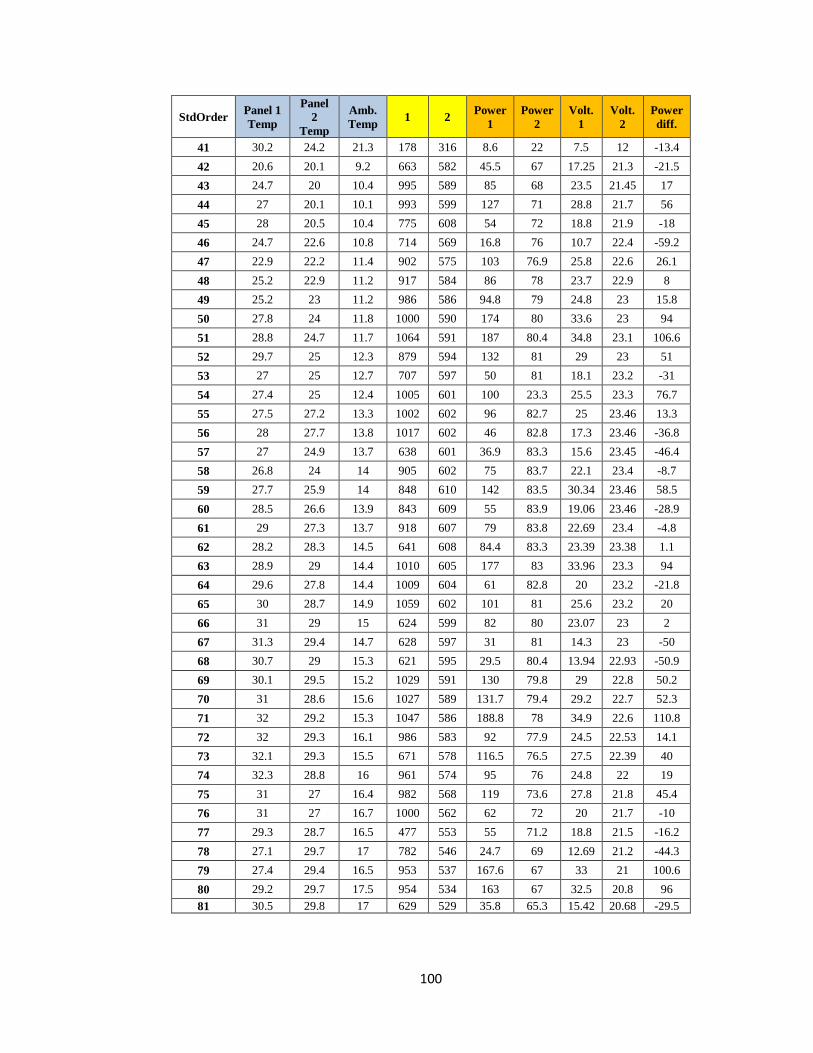
100
StdOrder Panel 1
Temp
Panel
2
Temp
Amb.
Temp 1 2
Power
1
Power
2
Volt.
1
Volt.
2
Power
diff.
41 30.2 24.2 21.3 178 316 8.6 22 7.5 12 -13.4
42 20.6 20.1 9.2 663 582 45.5 67 17.25 21.3 -21.5
43 24.7 20 10.4 995 589 85 68 23.5 21.45 17
44 27 20.1 10.1 993 599 127 71 28.8 21.7 56
45 28 20.5 10.4 775 608 54 72 18.8 21.9 -18
46 24.7 22.6 10.8 714 569 16.8 76 10.7 22.4 -59.2
47 22.9 22.2 11.4 902 575 103 76.9 25.8 22.6 26.1
48 25.2 22.9 11.2 917 584 86 78 23.7 22.9 8
49 25.2 23 11.2 986 586 94.8 79 24.8 23 15.8
50 27.8 24 11.8 1000 590 174 80 33.6 23 94
51 28.8 24.7 11.7 1064 591 187 80.4 34.8 23.1 106.6
52 29.7 25 12.3 879 594 132 81 29 23 51
53 27 25 12.7 707 597 50 81 18.1 23.2 -31
54 27.4 25 12.4 1005 601 100 23.3 25.5 23.3 76.7
55 27.5 27.2 13.3 1002 602 96 82.7 25 23.46 13.3
56 28 27.7 13.8 1017 602 46 82.8 17.3 23.46 -36.8
57 27 24.9 13.7 638 601 36.9 83.3 15.6 23.45 -46.4
58 26.8 24 14 905 602 75 83.7 22.1 23.4 -8.7
59 27.7 25.9 14 848 610 142 83.5 30.34 23.46 58.5
60 28.5 26.6 13.9 843 609 55 83.9 19.06 23.46 -28.9
61 29 27.3 13.7 918 607 79 83.8 22.69 23.4 -4.8
62 28.2 28.3 14.5 641 608 84.4 83.3 23.39 23.38 1.1
63 28.9 29 14.4 1010 605 177 83 33.96 23.3 94
64 29.6 27.8 14.4 1009 604 61 82.8 20 23.2 -21.8
65 30 28.7 14.9 1059 602 101 81 25.6 23.2 20
66 31 29 15 624 599 82 80 23.07 23 2
67 31.3 29.4 14.7 628 597 31 81 14.3 23 -50
68 30.7 29 15.3 621 595 29.5 80.4 13.94 22.93 -50.9
69 30.1 29.5 15.2 1029 591 130 79.8 29 22.8 50.2
70 31 28.6 15.6 1027 589 131.7 79.4 29.2 22.7 52.3
71 32 29.2 15.3 1047 586 188.8 78 34.9 22.6 110.8
72 32 29.3 16.1 986 583 92 77.9 24.5 22.53 14.1
73 32.1 29.3 15.5 671 578 116.5 76.5 27.5 22.39 40
74 32.3 28.8 16 961 574 95 76 24.8 22 19
75 31 27 16.4 982 568 119 73.6 27.8 21.8 45.4
76 31 27 16.7 1000 562 62 72 20 21.7 -10
77 29.3 28.7 16.5 477 553 55 71.2 18.8 21.5 -16.2
78 27.1 29.7 17 782 546 24.7 69 12.69 21.2 -44.3
79 27.4 29.4 16.5 953 537 167.6 67 33 21 100.6
80 29.2 29.7 17.5 954 534 163 67 32.5 20.8 96
81 30.5 29.8 17 629 529 35.8 65.3 15.42 20.68 -29.5

101
APPENDIX D. THE EFFICIENCY CALCULATIONS. THE EFFICIENCY
CALCULATED THROUGHOUT THE EXPERIMENT.
StdOrder Efficiency of Panel1
with irrediance2 as i/p Efficiency of Panel1 with
irrediance1 as i/p Efficiency of Panel2 with
irradiance 2 as i/p The gain in irradiance
in kW/m²
1 21.52% 15.48% 11.13% 254
2 9.71% 8.79% 11.21% 68
3 9.17% 6.77% 11.23% 233
4 23.30% 14.36% 11.21% 408
5 9.23% 5.83% 11.21% 382
6 12.86% 8.10% 11.28% 383
7 19.50% 13.49% 11.12% 291
8 10.69% 6.50% 11.19% 420
9 13.52% 8.31% 11.01% 405
10 10.09% 6.17% 10.79% 406
11 10.38% 6.57% 10.66% 365
12 13.35% 8.50% 10.48% 356
13 9.04% 7.55% 10.47% 121
14 14.92% 9.06% 10.27% 389
15 5.98% 6.00% 10.21% -2
16 4.24% 4.51% 9.99% -35
17 15.08% 8.58% 9.73% 437
18 3.78% 3.74% 9.63% 5
19 25.58% 15.34% 9.39% 370
20 4.03% 4.17% 9.51% -18
21 16.87% 9.12% 8.95% 443
22 17.33% 9.42% 9.20% 448
23 14.54% 8.22% 8.81% 394
24 4.48% 4.16% 8.70% 39
25 6.14% 5.76% 8.64% 32
26 5.19% 4.89% 8.34% 30
27 26.31% 13.84% 8.43% 421
28 15.63% 8.60% 8.11% 375
29 16.60% 8.58% 8.13% 422
30 15.52% 8.52% 7.66% 366
31 9.53% 10.19% 7.81% -28
32 3.64% 4.00% 7.72% -38
33 4.09% 5.16% 7.47% -85
34 14.80% 7.23% 7.49% 419
35 27.42% 14.30% 7.37% 354
36 8.85% 11.26% 7.02% -81
37 3.80% 6.10% 7.01% -138
38 12.82% 5.31% 6.71% 500
39 24.18% 8.58% 6.48% 616
40 6.84% 2.58% 6.43% 542

102
StdOrder Efficiency of Panel1
with irrediance2 as i/p
Efficiency of Panel1
with irrediance1 as i/p
Efficiency of Panel2 with
irradiance 2 as i/p
The gain in
irradiance in kW/m²
41 2.44% 4.33% 6.24% -138
42 7.01% 6.15% 10.32% 81
43 12.94% 7.66% 10.35% 406
44 19.01% 11.47% 10.63% 394
45 7.97% 6.25% 10.62% 167
46 2.65% 2.11% 11.98% 145
47 16.07% 10.24% 11.99% 327
48 13.21% 8.41% 11.98% 333
49 14.51% 8.62% 12.09% 400
50 26.45% 15.61% 12.16% 410
51 28.38% 15.76% 12.20% 473
52 19.93% 13.47% 12.23% 285
53 7.51% 6.34% 12.17% 110
54 14.92% 8.92% 3.48% 404
55 14.30% 8.59% 12.32% 400
56 6.85% 4.06% 12.34% 415
57 5.51% 5.19% 12.43% 37
58 11.17% 7.43% 12.47% 303
59 20.88% 15.02% 12.28% 238
60 8.10% 5.85% 12.36% 234
61 11.67% 7.72% 12.38% 311
62 12.45% 11.81% 12.29% 33
63 26.24% 15.72% 12.30% 405
64 9.06% 5.42% 12.29% 405
65 15.05% 8.55% 12.07% 457
66 12.28% 11.79% 11.98% 25
67 4.66% 4.43% 12.17% 31
68 4.45% 4.26% 12.12% 26
69 19.73% 11.33% 12.11% 438
70 20.05% 11.50% 12.09% 438
71 28.89% 16.17% 11.94% 461
72 14.15% 8.37% 11.98% 403
73 18.08% 15.57% 11.87% 93
74 14.84% 8.87% 11.87% 387
75 18.79% 10.87% 11.62% 414
76 9.89% 5.56% 11.49% 438
77 8.92% 10.34% 11.55% -76
78 4.06% 2.83% 11.33% 236
79 27.99% 15.77% 11.19% 416
80 27.38% 15.32% 11.25% 420
81 6.07% 5.10% 11.07% 100

103
REFERENCES
Aliexpress.com. (2016). Buy Products Online from China Wholesalers at Aliexpress.com.
Retrieved 30 January 2016, from http://www.aliexpress.com/item/Adjustable-
300W-10-ohm-Tube-Resistors-300-Watt-Wirewound-Ceramic-Resistance-on-
Sales/32341039664.html
Anderson, M.C. (2010) U.S. Patent No. 2010/0139735. Washington, DC: U.S. Patent and
Trademark Office.
Anthony, J. (1988). U.S. Patent No. 4,728,878. Washington, DC: U.S. Patent and
Trademark Office.
Boylestad, R. L., & Nashelsky, L. (1996). Electronics: A Survey of Electrical
Engineering Principles (4th Ed.). Englewood Cliffs, NJ: Prentice Hall.
Butler, D. M. (1978). U.S. Patent No 4,075,034. Washington, DC: U.S. Patent and
Trademark Office.
Cano, J. (2011). Photovoltaic Modules: Effect of Tilt Angle on Soiling. (Master’s thesis),
Engineering Technology, Arizona State University, Arizona.
Central Electricity Regulatory Commission. (2011). Performance of Solar Power Plants
in India, New Delhi, India: http://www.cercind.gov.in
Chiras, D. (2011). The homeowner’s guide to renewable energy. Gabriola Island, Canada:
New Society Publishers.
CRmagnetics Inc. (n.d.). DC Current Transducer [Brochure]. St. Louis, MO:
CRmagnetics Inc.

104
Daniel Sullivan. (2014, July 28). The danger of micro inverters [Web log post]. Retrieved
from http://www.sullivansolarpower.com/about/solar-power-blog/daniel-
sullivan/dangers-of-micro-inverters
Dorobantu, L., Popescu, M. O., Popescu, C., Craciunescu, A, (2011). “The Effect of
surface Impurities on Photovoltaic Panels,” International Conference on
Renewable Energy and Power Quality.
eGauge systems LLC. (2015). eGauge Model EG30xx Owner’s Manual(v1.0)
[pamphlet]. Boulder, CO: eGauge Systems LLC.
Ford, J. (2004). U.S. Patent No. 6,774,299 Washington, DC: U.S. Patent and Trademark
Office.
Goswami, Y., Kreith, F., & Kreider, F. (2000). Principles of solar engineering (2nd Ed.).
New York, NY: Taylor & Francis Group.
GreenRay, Inc. (2010). Sunsine 200 ac module. Retrieved from
http://www.greenraysolar.com/sites/default/files/GreenRay-SunSine200ACMod.p
He, G., Zhou, C., and Li, Z. (2010). “Review of Self-Cleaning Method for Solar Cell
Array.” Elsevier.
Help. (2016). Egauge7056.egaug.es. Retrieved 25 March 2016, from
http://egauge7056.egaug.es/help.html
Honsberg, C. & Bowden, S. (N. D.). Degradation and Failure Modes. Retrieved from:
http://pveducation.org/pvcdrom/modules/degradation-and-failure-modes
Hsieh, J. (1986). Solar energy engineering. Englewood Cliffs, N.J.: Prentice-Hall.

105
Jaiganesh, K. & Duraiswamy, K, (2013). “Improving the Power Generation from Solar
PV Panel Combined with Solar Thermal System for Indian Climatic Condition.”
International Journal of Applied Environmental Sciences (ISSN 0973-6077).
Volume, Number 6.
Jordan, D. C., & Kurtz, S. R. (2013). Photovoltaic Degradation Rates-an Analytical
Review. Progress In Photovoltaics, 21(1), 12-29. doi:10.1002/pip.1182
Kaplani, E. (2012). Detection of Degradation Effects in Field-Aged c-Si Solar Cells
through IR Thermography and Digital Image Processing. International Journal Of
Photoenergy, 1-11. doi:10.1155/2012/396792
Lam, W. (2009). Should You Spring Clean Your Solar Panels. Google official blog.
Retrieved from https://googleblog.blogspot.com/2009/07/should-you-spring-
clean-your-solar.html
Livingonsolarpower. (2013, June 10). Solar PV Power Plants: Major Causes of
Performance Degradation [Blog Post]. Retrieved From:
https://livingonsolarpower.wordpress.com/2013/06/10/solar-pv-power-plants-
major-causes-of-performance-degradation/
Mani, M. & Pillai, R. (2010). Impact of Dust on Solar Photovoltaic (PV) Performance:
Research Status, Challenges and Recommendations. Elsevier.
Marten, K., Rau, U. (2007). Renewable energy. M. Kaltschmitt, W. Streicher, & A.
Wiese(Ed.). Heidelberg, Germany: Springer.

106
Mazumder, M., Horenstein, M., Stark, J., Girouard, P., Sumner, R., Henderson, B.,
Sadder, O., Hidetaka, I.z, A., & Sharma, R. (2011). “Characterization of
Electrodynamic Screen Performance for Dust Removal from Solar Panels and
Solar Hydrogen Generators.” IEEE.
Mekhilef, S., Saidur, R., Kamalisarvestani, M, (2012). “Effect of Dust, Humidity and Air
Velocity on Efficiency of Photovoltaic Cells.” Elsevier.
Moharram, K. A., Abd-Elhady, M. S., Kandil, H. A., and Elsherif, H. (2013). “Influence
of Cleaning Using Water and Surfactants on the Performance of Photovoltaic
Panels.” Elsvier.
Mondol, J. D., Yohanis, Y. G., Norton, Y. B. (2006). “The Impact of Array Inclination
and Orientation on the Performance of a Grid-Connected Photovoltaic System.”
Elsevier.
Montgomery, D. (1997). Design and analysis of experiments. New York: Wiley.
Myers, R. H., & Montgomery, D. C. (2002). Response surface methodology: process and
product optimization using designed experiments. New York: J. Wiley, c2002.
National Renewable Energy Laboratory (2015), Efficiency chart [online image].
Retrieved from www. Nrel.gov/ncpv/images/efficiency_chart.jpg
Neitzel, F. (2016). Solar Tracking, Solar Tracking Systems, Solar Trackers | We Catch
the Sun. Solar-tracking.com. Retrieved 20 March 2016, from http://www.solar-
tracking.com/
Odeh, S., & Behnia, M, (2009). “Improving Photovoltaic Module Efficiency Using Water
Cooling.” Tylor & Francis Group.

107
Oliver, J. A. (2013). U.S. Patent No. 8,492,929 B2. Washington, DC: U.S. Patent and
Trademark Office.
Prasad, R. D., (2011). Handbook of renewable energy technology. A. Zobaa, & R. C.
Bansal (Ed.). Toh Tuck Link, Singapore: World scientific publishing Co. Pte. Ltd.
Rabinowitz, M. (2005). U.S. Patent No. 2005/0034750. Washington, DC: U.S. Patent and
Trademark Office.
Rajput, D., & Sudhakar, K. (2013). “Effect of Dust on the Performance of Solar PV
Panel.” International Conference on Global Scenario in Environment and Energy.
Schutten, H. P., Benjamin, J. A., & Lade, R. W. (1986). U.S. Patent No. 4,577,052
Washington, DC: U.S. Patent and Trademark Office.
Shepherd, W., & Shepherd, D. W. (2014). Energy studies (3rd Ed.). London, England:
Imperial College Press.
Skoplaki, E. & Palyvos, J. A, (2008). “On the Temperature Dependence of Photovoltaic
Module Electrical Performance: A review of Efficiency/Power Correlations.”
Elsevier.
SMA America, LLC. (2011). Ambient Temperature Sensor Tempsensor-Ambient
Installation Guide [Pamphlet]. Denver, CO: SMA America, LLC.
SMA America, LLC. (2011). System Monitoring Sunny Senesorbox Installation Guide
[Pamphlet]. Denver, CO: SMA America, LLC.
SMA Solar Technology AG. (2009). System Monitoring PT100m-NR Installation Guide
[Pamphlet]. Niestetal, Germany: SMA Solar Technology AG.

108
Smee, A. (1849). Elements of electro-biology, or, The voltaic mechanism of man.
London: Longman, Brown, Green & Longmans.
Solar Systems USA Online Solar Panels. (2016). Pallet of Eoplly 190 Watt Mono Solar
Panel. Retrieved 30 January 2016, from http://www.solarsystems-
usa.net/solarpanels/eoplly/ep125m-72-190/
Sørensen, B. (2011). Renewable energy. Burlington, MA: Academic Press.
Sulaiman, S. A., Singh, A. K., Mokhtar, M. M. M., Mohammed, A. B, (2014). Influence
of Dirt Accumulation on Performance of PV Panels. Elsevier.
Surles, W., Baum, J., Watrous, A., Johnson, S., Horanyi, E., Zarske, M. S, (2009).
“Photovoltaic Efficiency Lesson 2 the Temperature Effect”. Regents of the
University of Colorado. Retrieved from:
https://www.teachengineering.org/collection/cub_/lessons/cub_pveff/Attachments
/cub_pveff_lesson02_fundamentalsarticle_v6_tedl_dwc.pdf
Tester, J., Drake, E., Driscoll, M., Golay, M., & Peters, W. (2012). Sustainable energy:
Choosing among options (2nd Ed.). Cambridge, MA: The MIT Press.
The nobel prize, n.d. Retrieved from
http://www.nobelprize.org/nobel_prizes/physics/laureates/1921/
Ulrich, K., & Eppinger, S. (2012). Product design and development. New York:
McGraw-Hill/Irwin.
What Is A Response Surface Design? - Minitab. Support.minitab.com. N.p., 2016. Web.
21 Mar. 2016.

109
Zorrilla-Casanova, J., Piliougine, M., Carretero, J., Bernoaola, P., Carpena, P., Mora-
Lopez, L. & Sidrach-de-Cardona, M. (2011). “Analysis of Dust Losses in Photovoltaic
Modules.” World Renewable Energy Congre