i

UNIVERSITÉ DE LIÈGE

DDééppaarr tteemmeenntt SScc iieenncceess eett GGeesstt iioonn ddee ll ’’EEnnvvii rroonnnneemmeenntt

UUnnii ttéé AAssssaaiinniisssseemmeenntt eett EEnnvvii rroonnnneemmeenntt

OPTIMIZATION OF PARTIAL NITRIFICATION and DENITRIFICATION

PROCESSES IN

LANDFILL LEACHATE TREATMENT USING SEQUENCING BATCH REACTOR TECHNIQUE

Thesis presented for obtaining the degree of DOCTOR OF SCIENCES Speciality: Sciences and Sanitary of the Environment

by

HOANG Viet YenHOANG Viet YenHOANG Viet YenHOANG Viet Yen

Promoters: Prof. JeanProf. JeanProf. JeanProf. Jean----Luc VASELLuc VASELLuc VASELLuc VASEL Prof. LE Van CatProf. LE Van CatProf. LE Van CatProf. LE Van Cat

Jury members:

Prof. M. CRINEProf. M. CRINEProf. M. CRINEProf. M. CRINE - University of Liege (President) Prof. M. CARNOLProf. M. CARNOLProf. M. CARNOLProf. M. CARNOL - University of Liege DrDrDrDr. M. Th. BOUCHEZ. M. Th. BOUCHEZ. M. Th. BOUCHEZ. M. Th. BOUCHEZ - Antony, France Prof. JProf. JProf. JProf. J----L. VASELL. VASELL. VASELL. VASEL - University of Liege

Prof. LE V. C.Prof. LE V. C.Prof. LE V. C.Prof. LE V. C. - Vietnamese Academy of Science & Technology Prof. L. VANDEVENNEProf. L. VANDEVENNEProf. L. VANDEVENNEProf. L. VANDEVENNE - CEBEDEAU

December 2009

i

Acknowledgment

Above all, I would like to express my sincere thanks to my two Promoters,

Prof. Jean-Luc Vasel and Prof. Le Van Cat for their whole-hearted guidance

and support throughout my research. Your advices and comments in each and

every period are the most valuable contribution to my work.

I would like to thank very much to the jury members: Prof. M. Crine, Prof. M.

Carnol, Dr. M. Th. Bouchez, Prof. L. Vandevenne for your precious time in

reading and evaluating my work. The whole work could not be realized without the financial help from the

Belgian Technical Cooperation (BTC-CTB). I am so thankful for what your

staff have done for me beyond administrative stuff, especially Mrs. Liesbet

Vastenavondt has been very kind to me.

It’s an honor to have the University of Liege (ULG) received me.

Hanoi Urban Environment Company (URENCO) has been my base in many

senses for giving me good conditions to start and greatly helping me in

collecting documents and leachate for my study. I could not forget all colleagues who worked with me in the laboratories, in

Vietnam and in Belgium. Your supports, encouragements and friendships have

lifted me up in difficult times.

A special thank to Mr. Hugues Jupsin for his kind and very important support,

especially in technical issues. A special thank to Ms. Corine Antoine for her

enthusiasm helps with administrative procedures.

I would like to thank the members of the Laboratory of the Water Resources,

ULg, especially Mr. Serge Martin for their kind supports in analyzing the

wastewater samples. My sincere thanks also must be sent to Mr. Enrico Remigi (MOSTforWATER)

who supported me very much with the simulation sorfware WEST.

Last but not least, my great thanks to all members of my family, my best

friends for their always being by my side, encouraging and supporting me

during this hard period.

This work could not be done without you!

iii

Summary

Chapter I firstly presents general information about landfill leachate, focusing on formation and evolution of substrates in leachate. Then, landfill leachates in Vietnam are characterised, including raw leachates and leachates in biological ponds where they are normally collected to do experiments, short tests or long period experiments. Finally, general leachates treatment situation in Vietnam is reviewed, showing the pressing requirements for studies on leachate treatment. In chapter II, a careful bibliographical study on biological processes of nitrification and denitrification is done. Firstly, concept of microbiology and processes of nitrification and denitrification are reviewed, focusing on general process, microorganisms who directly participate in the processes, stoichiometry, kinetic, influences of the environmental factors on the processes. Secondly, literatures on partial nitrification and denitrification are studied, with recent approaches including normal partial nitrification, SHARON, ANAMMOX, CANON and SND. Also included in this part, studies on operating conditions (oxygen, pH, temperature…) for partial nitrification are presented, and based on that, experiments with real leachate will be implemented, which are given in the next chapters. In chapter III, existing activated sludge models are briefly reviewed, continuing by a comparison between ASM 1 (the first model and the foundation of the following models) and ASM3 (the model that will be modified to the new model for calibration - ASM3_2step). The ASM3 model then is studied in more detail with focuses on state variables, processes; kinetic and stoichiometric parameters of the model. A careful bibliographical study on sequencing batch reactor (SBR) is done in chapter IV. Firstly, a definition of an SBR is given with general information of the equipment, processes occurring and a comparison with conventional plants. Then, processes in an SBR (including fill, react, settling, draw and idle) are described. Information about advantages and disadvantages of the SBR technique are also given as a reason of choosing it for this study. Then, the processes in SBR are studied in more detail with their operating characteristics, focusing on equations of hydraulic parameters of an SBR. The literature of design of activated sludge SBR system is also required to support for setting up an SBR bench-scale that will be used for the experiments. To have ideas about the studied biological processes occurring in the studied technique (SBR) and how to apply mathematic models, literatures in SBR application for nitrogen removal; partial nitrification/denitrification and mathematical modelling nitrification/denitrification in SBR are reviewed. Chapter V presents materials and methods that will be applied in the experiments in laboratories and modelling processes of this study. The materials include leachate, biomass, chemicals, SBR bench-scale, bio-reactors, and WEST program, being described briefly in this chapter and in detail in each relating experiment. The methods include methodologies to determine the hydrodynamic and biological processes of SBR, data analysis and experimental planning, modelling and calibration protocols, model based optimisation and experimental approach. In chapter VI, a first experimental work is done in the laboratory in Belgium as first step of the study, before doing the experiments with the real leachate in Vietnam. Based on the studies on the SBR (Chapter IV), an SBR bench-scale is set up in the laboratory to study

iv

partial nitrification process, focusing on the SHARON process with a hope that the products of this process would be input for the ANAMMOX. This part is presented in the form of a paper, which was presented in The 5th Asian-Pacific Landfill Symposium in Sapporo (APLAS), 2008. This includes objectives, materials, results and discussions, and conclusions. Two main results that are given and discussed are mathematical model and optimization of the partial nitrification. Based on mathematical models derived from generally accepted ASM Model, specific growth rates of biomass (µ(T)) are found. Concentration of the active part of these four kinds of bacteria is also estimated and this will be applied as a method to estimate active biomass concentration in the next experiments. Optimisation process is done with different oxygen concentration and different working cycle mechanism. The first part of chapter VII presents the experimental studies on maximum nitrification and denitrification capability. The main achievements of this part are given in “Results and discussion”. The second part of the study is determination of kinetic and stoichiometric parameters that will be used for calibration in the next steps (Chapter IX). The main kinetic and stoichiometric parameters found from these tests include maximum growth rate, decay rate and yield coefficient of ammonium oxidizing bacteria, nitrite oxidizing bacteria and yield coefficient of heterotrophic bacteria. Chapter VIII presents a study on partial nitrification by applying data analysis and experimental planning method. This work is also the content of a paper that has been presented in the Twelfth International Waste Management and Landfill Symposium, Sardinia, October 2009. It consists of “Materials”, “Data analysis and planning of experiments”, “Results and discussions” and “Conclusions”. The most important parts in “Results and discussion” are observations and discussions in “Ammonium uptake rate, nitrite production rate, nitrate production rate, biomass activity and NO2/(NO2+NO3) ratio” and “Data analysis and establishment of recurrent equations of influencing factors”. In chapter IX, the modelisation of the partial nitrification and denitrification in SBR is presented. Firstly, materials used for the lab experiments and modelisation are described. The materials include SBR bench-scales, leachate and activated sludge, chemicals and modelling software - WEST program. Secondly, the applied calibration protocol is presented and has been used as a guideline throughout the calibration process. Thirdly, “Implementation of calibration process”, the main part of the chapter is presented. Following step by step the calibration protocol, the calibration process is implemented through six stages, including stage I “Target definition and information”; stage II “Plan survey and data analysis”, stage III “Model structure and process characterization”; stage IV “Calibration and validation”; stage V “Scenario analysis and optimisation”; and stage VI “Evaluation”. Each stage is divided into two or three sub-steps. The main results of the chapter are found in stage IV and V. In stage IV, calibration and validation results for (1)“Nitrification and denitrification without external carbon added in Vietnam”; (2) “Nitrification and denitrification with external carbon added in Vietnam” and (3) “Nitrification and denitrification with external carbon added in Belgium”. In stage V, there are two steps “Scenario analysis” and “Optimisation” that are done in Vietnam. It is hoped that, this study will contribute to the major issue of leachate treatment in Vietnam, especially in the North of the country where leachate characteristics and variations are very similar to those used during our experiments. Partial nitrification seems to be easily achieved in an SBR bench-scale using leachate in Nam Son landfill site, Hanoi, Vietnam. Some important characteristics of the studied

v

leachate, are high alkalinity, high pH leading to high free ammonia concentration in the system. This free ammonia is known as a growth rate inhibitor for nitrite oxidizing bacteria, thus limiting oxidation of nitrite to nitrate and accumulating nitrite during the nitrification period. DO concentration is also known as an important influencing factor in partial nitrification in many previous studies. But in our case, its influence is just significant when the nitrification process is nearly complete: no more ammonium remains in the system, alkalinity concentration is reduced leading to a lower buffer capacity, lower pH, and then nitrite is easily oxidized to nitrate. A sufficiently high DO concentration in this case, expresses its importance in bringing about the best nitrification efficiency, while saving aeration energy. The SBR technique has demonstrated its advantages in this study, especially the flexibility in changing the working volume, and the operating time mechanism. The automatic SBR bench-scale used in the lab experiments has functioned very well, easy to operate and to control. Modelisation of partial nitrification and denitrification processes for landfill leachate treatment using the Sequencing Batch Reactor technology was the main objective of this study. The simulation software - WEST® program was a very useful tool to implement this task. With this program, the available model base for activated sludge model (ASM1, ASM 2, ASM 3 etc,), presented in the Peterson matrix, the variables, kinetic, stoichiometric parameters, processes can be easily modified to another activated sludge model suitable in the scope of our study. In the present case, based on the ASM3, the ASM3_2step was developed and applied, in which nitrification and denitrification are divided into two steps with nitrite as an intermediate product. The modified ASM3_2step has shown its high accuracy during calibration process. It could be used also for the other techniques using activated sludge, not only for an activated sludge SBR. On the other hand it is adding more equations and consequently more parameters. Calibration and validation processes were implemented for two cases: Nitrification and denitrification with and without carbon addition in Vietnam and in Belgium. Good results were obtained where the simulations fit well the experimental data. The kinetic and stoichiometric parameters found from the calibration and validation (at steady state) were very important for the other simulations, especially in process optimisation. The process simulation is also very important in predicting the development of the treatment process. Based on the simulation profile, one can look back to the conditions of the experiments to find out if there is something wrong in the system, providing interesting tools to improve the operating conditions of the system. It also has been demonstrated that, through scenario analysis and optimisation of the process, general productivity of the SBR system can be increased. Changing operating time cycle mechanisms by reducing the aeration time and increasing the time for anoxic phase can improve the total nitrogen removal efficiency, save some energy related to aeration for nitrification and save also the carbon source for denitrification. The experiments were implemented in the SBR bench-scale, which is small lab equipment. It is obvious that there will be differences when working with a real scale SBR plant, with large climate variations, with big variation of input leachate (characteristic as well as flowrate). However, the results of modelisation in this study could be a good start for simulation and optimization of an existing SBR plant (of the same type) or also for development of a new one.

vi

As our results are very promising the next step could be to implement the anammox process. As we now control the conditions to reach an appropriate NH4/NO2 ratio to start an anammox process. Leachate treatment is a major issue in many countries and also in Vietnam as in other South East Asia countries where the very large pluviometry induced very large amounts of leachates but still at high concentrations. As everywhere in the world the major issue associated to leachate treatment is the treatment of the very high fluxes of the nitrogen contained in those leachates. We demonstrated that partial nitrification can be obtained and controlled on a batch scale system which offers a rather simple and efficient way to implement leachate treatment. Obviously the batch mode associated to the SBR process is very useful to get and to maintain the partial nitrification process, probably in a more simple and efficient way than a continuous process.

vii

Résumé

Les informations générales disponibles au sujet des lixiviats de CET, se concentrant sur la formation et l'évolution des substrats dans le lixiviat sont présentées au chapitre I. Puis, les lixiviats de CET au Vietnam sont caractérisés, y compris les lixiviats bruts et les lixiviats stockés dans les étangs biologiques où ils sont normalement collectés pour faire des expériences, des essais courts ou des expériences de longue période. En conclusion, la situation générale de traitement des lixiviats au Vietnam est passée en revue, confirmant les pressions croissantes pressantes pour des études sur le traitement de lixiviat. En chapitre II, une étude bibliographique soigneuse sur les processus biologiques de nitrification et la dénitrification est faite. Premièrement, le concept de la microbiologie et les processus de nitrification et de dénitrification sont passés en revue, se concentrant sur le processus général, les micro-organismes qui participent directement aux processus, stœchiométrie, cinétique, influences des facteurs environnementaux sur les processus. Deuxièmement, la littérature sur la nitrification et la dénitrification partielle est étudiée, avec des approches récentes comprenant la nitrification partielle normale, le SHARON, l'ANAMMOX, le CANON et le SND. Est également incluse dans la présente partie, l’effet des conditions opératoires (l'oxygène, pH, la température…) sur la nitrification partielle que serviront de base pour les expériences avec le lixiviat réel présentées dans les chapitre suivants. En chapitre III, des modèles existants de boue activée sont brièvement passés en revue, en poursuivant par une comparaison entre l'ASM 1 (le premier modèle et la base des modèles suivants) et l'ASM3 (le modèle qui sera modifié selon le nouveau modèle pour le calibrage - ASM3_2step). Le modèle ASM3 alors est étudié plus avant en détaillant variables d'état, processus ; paramètres cinétiques et stœchiométriques du modèle. Une étude bibliographique soigneuse sur le système SBR est faite en chapitre IV. Premièrement, une définition d'un SBR est donnée avec des informations générales de l'équipement, de l'occurrence des processus et d'une comparaison avec les systèmes conventionnels. Puis, les processus dans un SBR (remplissage, réaction, arrêt, décantation, repos) sont décrits. Des informations sur les avantages et les inconvénients de la technique SBR sont également donnés justifiant cette étude. Puis, les processus dans SBR sont étudiés en plus détail avec leurs caractéristiques de fonctionnement, se concentrant sur le brassage du SBR et les transferts de matière. La littérature relative à la boue activée SBR est également utilisée pour concevoir un bench-scale SBR qui sera employé pour les expériences. Pour préciser les processus biologiques étudiés se produisant dans la technique étudiée (SBR) et comment appliquer les modèles mathématiques, la littérature relative au SBR en traitement de l’azote; la nitrification/dénitrification et la nitrification/dénitrification partielles, modélisation mathématique des sont passées en revue. Le chapitre V présente les matériaux et les méthodes qui seront appliqués dans les expériences de laboratoires et l’approche de modélisation de cette étude. Les matériaux incluent le lixiviat, la biomasse, les produits chimiques, le bench-scale SBR, les bioréacteurs, et le programme WEST, étant décrits brièvement en ce chapitre puis en détail dans chaque expérience. Les méthodes incluent des méthodologies pour déterminer les processus hydrodynamiques et biologiques des SBR, l’analyse de données et la planification expérimentale, l’optimisation basée sur la modélisation, puis le protocole de calibrage et de modélisation, et l’approche expérimentale.

viii

En chapitre VI, le travail est effectué dans le laboratoire en Belgique comme première étape de l'étude, avant de faire les expériences avec le lixiviat réel au Vietnam. Basé sur les études sur le SBR (chapitre IV), un bench-scale SBR est installé dans le laboratoire pour étudier le procédé partiel de nitrification, se concentrant sur le processus SHARON avec l’espoir que les produits de ce processus seraient ensuite l’objet du procédé 'ANAMMOX. La présente partie est sous forme d’article, qui a été présenté au «5th Asian-Pacific Landfill Symposium, Sapporo, 2008 (APLAS) ». Ceci inclut des objectifs, des matériaux, des résultats et des discussions, et des conclusions. Deux résultats principaux qui sont discutés: le modèle mathématique et l’optimisation de la nitrification partielle. Basé sur les modèles mathématiques on a dérivé du modèle courant ASM, les taux de croissance spécifiques de biomasse (µ(T)). La concentration de la fraction active de pour quatre genres de bactéries est également estimée et ceci sera appliqué estimer la concentration active de biomasse dans les prochaines expériences. Le processus d'optimisation est fait avec une concentration d’oxygène différente et un cycle de fonctionnement différent. La première partie du chapitre VII présente les études expérimentales sur des possibilités maximum de nitrification et de dénitrification. Les résultats principaux sont donnés dans «des résultats et discussions ». La deuxième partie de l'étude porte sur la détermination des paramètres cinétiques et stœchiométriques qui seront employés pour le calibrage dans les prochaines étapes (chapitre IX). Les paramètres cinétiques et stœchiométriques principaux provenant de ces essais incluent le taux de croissance maximum, le taux de décomposition et le coefficient de rendement des bactéries nitritantes et nitratantes, et le coefficient de rendement de bactéries hétérotrophes. Le chapitre VIII présente une étude sur la nitrification partielle en appliquant l'analyse de données et la méthode de planification expérimentale. Ce travail est également le contenu d'un article présenté au « Twelfth International Waste Management and Landfill Symposium, Sardinia, October 2009 ». Il se compose de l'analyse de « matériaux », « de données et de la planification des expériences », «des résultats et des discussions » et « des conclusions ». les principaux résultats portent sur “Ammonium uptake rate, nitrite production rate, nitrate production rate, l'activité de biomasse et le rapport de NO2/(NO2+NO3) » et la « analyse de données et l'établissement des équations récurrentes de l'influence factorise ». En chapitre IX, la modélisation de la nitrification partielle et la dénitrification dans SBR est présentée. Premièrement, des matières employées pour les expériences de laboratoire et la modélisation sont décrites. Les matériaux incluent bench-scale SBR, lixiviat et boue activée, produits chimiques et logiciel de modélisation - programme WEST. Deuxièmement, le protocole de calibrage est présenté ; il servira de base tout le procédé de calibrage. Troisièmement, la mise en œuvre du procédé de calibrage », la partie principale du chapitre est présentée. Le procédé de calibrage est mis en application en six étapes, y compris l'étape I « définition et information de cible » ; étape II « planning expérimental et analyse de données », étape III « structure du modèle et caractérisation des processus » ; étape IV « calibrage et validation » ; étape V « analyse de scénarios et optimisation » ; et étape VI « évaluation ». Chaque étape est divisée en deux ou trois sub-steps. Les résultats principaux du chapitre sont trouvés dans l'étape IV et V. Dans l'étape IV, il y a calibrage et validation qui sont faits pour (1) la « nitrification et la dénitrification sans carbone externe supplémentaire, au Vietnam » ; (2) la « nitrification et la dénitrification avec le carbone externe supplémentaire, au Vietnam » et (3) « nitrification et dénitrification avec le

ix

carbone externe supplémentaire, en Belgique ». Dans l'étape V, il y a deux étapes « analyse de scénario » et « optimisation » qui sont faites, au Vietnam.

On espère que, cette étude contribuera au thème important du traitement de lixiviat au Vietnam, particulièrement dans le nord du pays où les caractéristiques et les variations de lixiviat sont très similaires à ce qui a été employé pendant nos expériences. La nitrification partielle semble être facilement obtenue dans un bench-scale SBR utilisant le lixiviat du CET de Nam Son, Hanoi, Vietnam. Nous considérons cela en raison de caractéristiques importantes du lixiviat étudié telles que l'alcalinité élevée, le pH élevé associé à la concentration élevée en ammoniaque libre dans le système. Cette ammoniaque libre est connu comme inhibiteur du taux de croissance des nitratantes. La concentration en oxygène dissous est également connue comme un facteur d’influence important dans la nitrification partielle dans beaucoup d'études précédentes. Mais dans notre cas, son influence est simplement significative lorsque le procédé de nitrification est presque complet: l’ammonium ne reste plus dans le système, alcalinité est réduite de ce fait le pouvoir tampon, le pH est bas, alors le nitrite est facilement oxydé en nitrate. Une concentration d’oxygène suffisante dans ce cas-ci, exprime son importance en induisant une meilleure efficacité de nitrification, tout en économisant l'énergie d'aération. La technique de SBR a démontré ses avantages dans cette étude, particulièrement: la flexibilité du volume de travail, et le temps de travail. Le SBR bench-scale automatique utilisé dans les expériences de laboratoire a fonctionné très bien, il est facile à utiliser et contrôler. La modélisation des procédés partiels de nitrification et de dénitrification pour le traitement de lixivias de CET utilisant la technique SBR était l'objectif principal de cette étude. Le logiciel de simulation - le programme de WEST® s’est avéré un outil très utile pour mettre en application cette tâche. Avec ce programme, la base modèle disponible pour le modèle de boue activée (ASM1, ASM 2, ASM 3 etc.,), présentée dans la matrice de Peterson, les variables, les paramètres cinétiques et stœchiométriques, les processus peuvent être modifiés facilement pour un autre modèle de boue activée dans la portée de notre étude. Dans le cas actuel, basé sur l'ASM3, l'ASM3_2step a été développé et appliqué, dans lequel la nitrification et la dénitrification sont divisées en deux étapes avec le nitrite comme produit intermédiaire. L'ASM3_2step modifié a montré son grande précision pendant le procédé de calibrage. Il pourrait être utilisé également pour les autres techniques utilisant la boue activée, non seulement pour une boue activée SBR. Par contre cela ajoute plus d'équations et par conséquent plus de paramètres. Des procédés de calibrage et de validation ont été mis en application pour deux cas : Nitrification et dénitrification avec et sans l'addition de carbone, au Vietnam et en Belgique. De bons résultats ont été obtenus où les simulations confirment les données expérimentales. Les paramètres cinétiques et stœchiométriques trouvés lors du calibrage et de la validation (à l’équilibre) sont très importants pour les autres simulations, particulièrement dans l'optimisation du processus. La simulation de processus est également très importante en prévoyant les schémas possibles des processus de traitement. Basé sur le profil de simulation, on peut examiner de nouveau aux conditions des expériences pour découvrir mieux cerner les difficultés, fournissant des outils intéressants pour améliorer les conditions de fonctionnement du système.

x

On a démontré également que, par l'analyse de scénario et l'optimisation du processus, la productivité générale du système de SBR peut être augmentée. L’adaptation des cycles de temps de travail en réduisant le temps d'aération et en augmentant la durée de la phase anoxique peuvent améliorer toute l'efficacité d'élimination de l’ azote, économisant l’énergie d’aération pour la nitrification et économisant également la source de carbone pour la dénitrification. Les expériences ont été mises en application dans le bench-scale SBR, qui reste un petit équipement de laboratoire. Il est évident que, il y aura des différences en travaillant à taille réelle SBR, avec de grandes variations climatiques, associées aux grandes variations du lixiviat d'entrée (caractéristiques aussi bien que débit). Cependant, les résultats de la modélisation dans cette étude constituent un bon début pour la simulation et l’optimisation d'une installation existante de SBR (du même type) ou également pour le développement de nouvelles unités. Nos résultats étant très prometteurs, la prochaine étape pourrait être de mettre en application le processus Anammox puisque nous maitrisons maintenant les conditions pour atteindre un rapport NH4/NO2 approprié pour commencer un processus d'anammox. Le traitement de lixiviat est une problématique très importante dans beaucoup de pays, également au Vietnam comme dans d'autres pays d'Asie du Sud-Est où la pluviométrie très grande induit de très des grands volumes de lixiviats mais toujours à des concentrations élevées. Comme partout dans le monde, le thème principal associé au traitement de lixiviat est le traitement des flux très élevés en l'azote contenu dans ces lixiviats. Nous avons démontré que la nitrification partielle peut être obtenue et commandée sur un système de SBR qui offre une manière plutôt simple et efficace de mettre en œuvre le traitement de lixiviat. Évidemment l'exploitation par cuvées (discontinu) est associée au processus SBR est très utile pour obtenir et maintenir le procédé partiel de nitrification, probablement d'une manière plus simple et plus efficace que par un processus continu.

xi

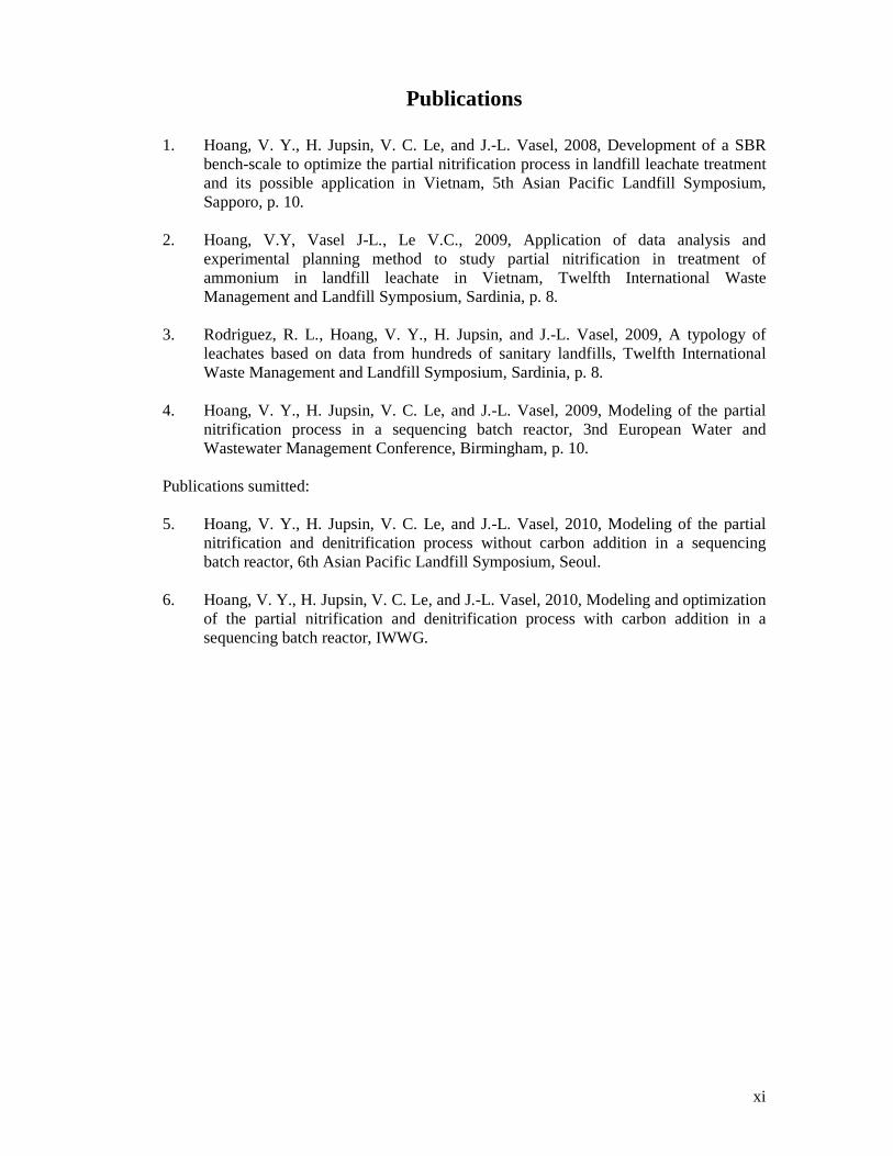
Publications

1. Hoang, V. Y., H. Jupsin, V. C. Le, and J.-L. Vasel, 2008, Development of a SBR bench-scale to optimize the partial nitrification process in landfill leachate treatment and its possible application in Vietnam, 5th Asian Pacific Landfill Symposium, Sapporo, p. 10.

2. Hoang, V.Y, Vasel J-L., Le V.C., 2009, Application of data analysis and

experimental planning method to study partial nitrification in treatment of ammonium in landfill leachate in Vietnam, Twelfth International Waste Management and Landfill Symposium, Sardinia, p. 8.

3. Rodriguez, R. L., Hoang, V. Y., H. Jupsin, and J.-L. Vasel, 2009, A typology of

leachates based on data from hundreds of sanitary landfills, Twelfth International Waste Management and Landfill Symposium, Sardinia, p. 8.

4. Hoang, V. Y., H. Jupsin, V. C. Le, and J.-L. Vasel, 2009, Modeling of the partial

nitrification process in a sequencing batch reactor, 3nd European Water and Wastewater Management Conference, Birmingham, p. 10.

Publications sumitted: 5. Hoang, V. Y., H. Jupsin, V. C. Le, and J.-L. Vasel, 2010, Modeling of the partial

nitrification and denitrification process without carbon addition in a sequencing batch reactor, 6th Asian Pacific Landfill Symposium, Seoul.

6. Hoang, V. Y., H. Jupsin, V. C. Le, and J.-L. Vasel, 2010, Modeling and optimization

of the partial nitrification and denitrification process with carbon addition in a sequencing batch reactor, IWWG.

xiii

TABLES OF CONTENTS

CHAPTER I .................................................................................................................... 1

BIBLIOGRAPHICAL STUDY: LANFILL LEACHATE AND CHARACTERISTICS OF LANDFILL LEACHATE IN VIETNAM.... ...................... 1

1.1. LANDFILL LEACHATE: FORMATION AND EVOLUTION OF

SUBSTRATES IN LEACHATE ....................................................................................... 1 1.2. CHARACTERISTICS OF LANDFILL LEACHATE IN VIETNAM .......................... 2 1.2.1. GENERAL CHARACTERISTIC OF RAW LANDFILL LEACHATE......................................... 2 1.2.2. CHARACTERISTIC OF LANDFILL LEACHATE AT BIOLOGICAL PONDS. ............................ 3

1.2.2.1. pH................................................................................................................. 5 1.2.2.2 Alkalinity ....................................................................................................... 5 1.2.2.3. Suspended solid ............................................................................................ 6 1.2.2.4. Volatile fatty acid (VFA) ............................................................................... 6 1.2.2.5. COD ............................................................................................................. 7 1.2.2.6. Nitrogen compound....................................................................................... 7 1.2.2.7. Phosphorus compound.................................................................................. 8

1.3. GENERAL OF LEACHATE TREATMENT IN VIETNAM....................................... 9 1.3.1. LEACHATE TREATMENT SYSTEMS IN NAM SON LANDFILL SITE, HANOI ...................... 9

1.3.1.1. Biological treatment system .......................................................................... 9 1.3.1.2. The system established by UCE..................................................................... 9 1.3.1.3. The system established by Mechanic and Aquiculture Company.................... 9 1.3.1.4. The system established by SEEN Company.................................................. 10

1.3.2. LEACHATE TREATMENT SYSTEMS IN PHUOC HIEP LANDFILL SITE, HO CHI MINH

CITY ................................................................................................................................ 10 1.3.2.1. The system established by Centre for Environment (CENTEMA)................. 10 1.3.2.2. The system established by Quoc Viet Company ........................................... 10 1.3.2.3. The system established by Duc Lam Ltd. Company ..................................... 10

REFERENCES ............................................................................................................... 11

CHAPTER II................................................................................................................. 13

BIBLIOGRAPHICAL STUDY: BIOLOGICAL PROCESSES OF NITRIFICATION AND DENITRIFICATION .................. ......................................... 13

2.1. CONCEPT OF MICROBIOLOGY AND PROCESSES OF NITRIFICATION

AND DENITRIFICATION............................................................................................. 13 2.1.1. NITRIFICATION ....................................................................................................... 13 2.1.1.1. DEFINITION ......................................................................................................... 13 2.1.1.2. NITRIFYING MICRO-ORGANISMS........................................................................... 13 2.1.1.3. STOICHIOMETRY OF NITRIFICATION...................................................................... 14 2.1.1.4. KINETICS OF NITRIFICATION................................................................................. 15 2.1.1.5. THE INFLUENCE OF THE ENVIRONMENTAL FACTORS ON NITRIFICATION .................. 17 2.1.2. DENITRIFICATION ................................................................................................... 26 2.1.2.1. DEFINITION ......................................................................................................... 26 2.1.2.2. DENITRIFYING MICRO-ORGANISMS....................................................................... 26 2.1.2.3. STOICHIOMETRY OF DENITRIFICATION.................................................................. 27 2.1.2.4. KINETICS OF DENITRIFICATION............................................................................. 28 2.1.2.5. THE INFLUENCE OF THE ENVIRONMENTAL FACTORS ON DENITRIFICATION .............. 30 2.2. PARTIAL NITRIFICATION AND DENITRIFICATION......................................... 32 2.2.1. SOME CONFIGURATIONS OF BIOLOGICAL PROCESSES APPLIED IN PARTIAL

NITRIFICATION/DENITRIFICATION...................................................................................... 32

xiv

2.2.1.1. CONVENTIONAL NITRIFICATION/DENITRIFICATION PROCESS..................................32 2.2.1.2. PARTIAL NITRIFICATION .......................................................................................32 2.2.1.3. SHARON (SINGLE REACTOR HIGH ACTIVITY AMMONIA REMOVAL OVER

NITRITE) PROCESS............................................................................................................34 2.2.1.4. ANAMMOX (ANAEROBIC AMMONIUM OXIDATION ) PROCESS.............................35 2.2.1.5. CANON (COMPLETELY AUTOTROPHIC NITROGEN REMOVAL OVER NITRITE) PROCESS..........................................................................................................................37 2.2.1.6. SND (SIMULTANEOUS NITRIFICATION DENITRIFICATION) PROCESS......................38 2.2.2. OPERATING CONDITIONS FOR PARTIAL NITRIFICATION..............................................39 2.2.2.1. DISSOLVED OXYGEN............................................................................................39 2.2.2.2. TEMPERATURE.....................................................................................................40 2.2.2.3. HYDRAULIC RETENTION TIME (HRT) AND SOLID RESIDENCE TIME (SRT) ..............40 2.2.2.4. PH, ALKALINITY AND NH3/HNO2........................................................................41 REFERENCE..................................................................................................................45

CHAPTER III ...............................................................................................................53

ACTIVATED SLUDGE MODELS .............................................................................53

3.1. ACTIVATED SLUDGE MODELS...........................................................................53 3.2. COMPARISON BETWEEN ASM1 AND ASM3......................................................53 3.3. ASM3 MODEL ........................................................................................................54 3.3.1. STATE VARIABLES IN ASM3 ...................................................................................54 3.3.2. PROCESSES IN ASM3..............................................................................................56 3.3.3. ESTIMATION OF KINETIC AND STOICHIOMETRIC PARAMETERS...................................58 REFERENCES ...............................................................................................................60

CHAPTER IV................................................................................................................61

BIBLIOGRAPHICAL STUDY: SEQUENCING BATCH REACTOR .... .................61

4.1. DEFINITION ...........................................................................................................61 4.2. PROCESS DESCRIPTION.......................................................................................61 4.3. ADVANTAGES AND DISADVANTAGES OF SBR...............................................64

4.3.1. Advantages .................................................................................................... 64 4.3.2. Disadvantages ............................................................................................... 65

4.4. OPERATING CHARACTERISTICS IN SBR PROCESS .........................................66 4.5. DESIGN OF ACTIVATED SLUDGE SBR SYSTEM...............................................68 4.6. SBR APPLICATION FOR NITROGEN REMOVAL ...............................................71 4.7. PARTIAL NITRIFICATION/DENITRIFICATION IN SBR.....................................76 4.8. MATHEMATICALLY MODELLING NITRIFICATION AND

DENITRIFICATION IN SEQUENCING BATCH REACTOR........................................77 REFERENCE..................................................................................................................80

CHAPTER V .................................................................................................................85

MATERIALS AND METHODS ..................................................................................85

5.1. MATERIALS ...........................................................................................................85 5.1.1. LEACHATE..............................................................................................................85 5.1.2. BIOMASS ................................................................................................................85 5.1.3. CHEMICALS: ...........................................................................................................85 5.1.4. SBR BENCH-SCALE.................................................................................................86 5.1.5. BIO-REACTOR FOR DETERMINATION OF MAXIMUM NITRIFICATION AND

DENITRIFICATION CAPABILITY AND KINETIC AND STOICHIOMETRIC PARAMETERS...............86 5.1.6. RESPIRATION REACTOR TO QUANTIFY STOICHIOMETRIC PARAMETERS......................86 5.1.7. WEST PROGRAM....................................................................................................86

xv

5.2. METHODS .............................................................................................................. 86 5.2.1. METHODS TO DETERMINE THE HYDRODYNAMIC AND BIOLOGICAL PROCESSES OF

SBR ................................................................................................................................ 86 5.2.1.1. Measurement of mass transfer coefficient gas-liquid Kla............................. 86 5.2.1.2. Tracer tests: measurements of the mixing time based on conductivity.......... 87 5.2.1.3. Respiration and biomass activity tests in the reactor with steady state biomass to fix mixing time and aeration periods in the SBR reactor ...................................... 88 5.2.1.4. Bioactivity tests to determine maximum nitrification and denitrification capability and some kinetic and stoichiometric parameters ..................................... 88 5.2.1.5. Determination of biomass proportion in an activated sludge sample ........... 90

FIGURE. 5.3. MNP TABLE .................................................................................................. 91 5.2.2. DATA ANALYSIS AND EXPERIMENTAL PLANNING ..................................................... 91 5.2.3. MODELLING AND CALIBRATION PROTOCOLS............................................................ 91

5.2.3.1. The existing calibration protocol for IWA models ....................................... 91 5.2.3.2. The common structure of calibration protocols ........................................... 94 5.2.3.3. Some main differences between calibration protocols ................................. 95

5.2.4. MODEL-BASED OPTIMIZATION................................................................................. 96 5.2.5. EXPERIMENTAL APPROACH..................................................................................... 96 REFERENCE ................................................................................................................. 97

CHAPTER VI ............................................................................................................... 99

SETTING UP AN SBR TO STUDY PARTIAL NITRIFICATION ... ........................ 99

6.1. OBJECTIVES .......................................................................................................... 99 6.1.1. THE MAIN OBJECTIVE.............................................................................................. 99 6.1.2. SPECIFIC OBJECTIVES.............................................................................................. 99 6.2. MATERIALS........................................................................................................... 99 6.2.1. LEACHATE AND ACTIVATED SLUDGE (BIOMASS) ...................................................... 99 6.2.2. CARBON SOURCE FOR DENITRIFICATION................................................................ 100 6.2.3. SBR BENCH-SCALE............................................................................................... 100 6.3. RESULTS AND DISCUSSION.............................................................................. 103 6.3.1. TRACER TESTS TO DETERMINE MIXING CAPACITY...................................................103 6.3.2. GAS-LIQUID MASS TRANSFER COEFFICIENTS KLA ...................................................103 6.3.3. RESPIRATION AND BIOMASS ACTIVITY................................................................... 104 6.3.4. SETTLING CAPACITY OF SLUDGE IN THE SYSTEM.................................................... 104 6.3.5. MATHEMATICAL MODEL ....................................................................................... 105 6.3.6. OPTIMIZATION OF THE PARTIAL NITRIFICATION...................................................... 107 6. 4. CONCLUSION OF THE CHAPTER ..................................................................... 110 REFERENCES ............................................................................................................. 111

CHAPTER VII............................................................................................................ 113

TESTS FOR DETERMINATION OF MAXIMUM NITRIFICATION AN D DENITRIFICATION CAPABILITY AND KINETIC AND STOICHIO METRIC PARAMETERS........................................................................................................... 113

7.1. TEST FOR DETERMINATION OF MAXIMUM NITRIFICATION AND

DENITRIFICATION CAPABILITY ............................................................................ 113 7.1.1. MATERIALS .......................................................................................................... 113 7.1.2. WORKING CONDITION........................................................................................... 114 7.1.3. RESULTS AND DISCUSSIONS................................................................................... 115 7.1.3.1. TEST TO DETERMINE THE MAXIMUM NITRIFICATION CAPABILITY IN B1................ 115 7.1.3.2. TESTS TO DETERMINE THE MAXIMUM DENITRIFICATION CAPABILITY IN B2 .......... 117

xvi

7.2. BIOACTIVITY ESSAYS TO DETERMINE KINETIC AND

STOICHIOMETRIC PARAMETERS OF ACTIVATED SLUDGE............................... 121 7.2.1. MATERIALS .......................................................................................................... 122 7.2.2. WORKING MECHANISM ......................................................................................... 122 7.2.3. RESULTS .............................................................................................................. 124 7.3. RESPIRATION TEST (FOR DETERMINATION OF HETEROTROPHIC YIELD

(YH).............................................................................................................................. 129 REFERENCES ............................................................................................................. 132

CHAPTER VIII........................................................................................................... 133

APLICATION OF DATA ANALYSIS AND EXPERIMENTAL PLANNI NG METHOD TO STUDY PARTIAL NITRIFICATION.............. ................................ 133

8.1. MATERIALS ......................................................................................................... 133 8.1.1. LEACHATE AND ACTIVATED SLUDGE ..................................................................... 133 8.1.2. ACTIVATED SLUDGE ............................................................................................. 133 8.1.3. CHEMICALS .......................................................................................................... 134 8.14. SINGLE REACTOR................................................................................................... 134 8.1.5 ONLINE MEASUREMENT ......................................................................................... 134 8.2. DATA ANALYSIS AND PLANNING OF EXPERIMENTS .................................. 134 8.3. RESULTS AND DISCUSSIONS............................................................................ 135 8.3.1. TRACER TEST TO DETERMINE MIXING CAPABILITY OF THE SYSTEM ......................... 135 8.3.2. GAS-LIQUID MASS TRANSFER COEFFICIENTS KLA ...................................................136 8.3.3. RESPIRATION RATE OF BIOMASS............................................................................ 137 8.3.4. AMMONIUM UPTAKE RATE (AUR), NITRITE PRODUCTION RATE (NPR1), NITRATE

PRODUCTION RATE (NPR2), BIOMASS ACTIVITY (BA) AND NO2-/(NO2-+NO3-) RATIO ... 139 8.3.5. DATA ANALYSIS AND ESTABLISHMENT OF RECURRENT EQUATIONS OF

INFLUENCING FACTORS................................................................................................... 143 8.4. CONCLUSIONS .................................................................................................... 145 REFERENCES ............................................................................................................. 146

CHAPTER IX.............................................................................................................. 147

MODELISATION OF PARTIAL NITRIFICATION AND DENITRIFI CATION IN SBR .............................................................................................................................. 147

9.1. MATERIALS ......................................................................................................... 147 9.1.1. SBR BENCH-SCALES............................................................................................. 147 9.1.2. LEACHATE AND ACTIVATED SLUDGE ..................................................................... 151 9.1.3. CHEMICALS .......................................................................................................... 152 9.1.4. SIMULATION SOFTWARE - WEST PROGRAM........................................................... 153 9.2. APPLICATION OF CALIBRATION PROTOCOL ................................................ 153 9.3. IMPLEMENTATION OF CALIBRATION PROCESS........................................... 155 9.3.1. STAGE I: TARGET DEFINITION AND INFORMATION ................................. 155

Step 1. Target definition......................................................................................... 155 Step 2. Decision about the information needed ...................................................... 155

9.3.2. STAGE II: PLAN SURVEY AND DATA ANALYSIS ........................................ 157 Step 3. Plant survey ............................................................................................... 157 Step 4. Data analysis ............................................................................................. 163

9.3.3. STAGE III: MODEL STRUCTURE AND PROCESS CHARACTERIZATION ..163 Step 5. Model definition......................................................................................... 163 5.a. Mass transfer.................................................................................................. 163 5.b. Settler ............................................................................................................. 164 5.c. Mixing capability ............................................................................................ 166

xvii

5.d. Selecting the biological model .........................................................................166 Step 6. Process characterization.............................................................................175 6.a. Estimation of ASM parameters ........................................................................175 6.b. Determination of sludge concentration and biomass fractionation...................175 6.c. Influent wastewater characterization ...............................................................177

9.3.4. STAGE IV: CALIBRATION AND VALIDATION ............................................. 181 9.3.4.1. NITRIFICATION AND DENITRIFICATION WITHOUT EXTERNAL CARBON ADDITION ... 181

Step 7A. Calibration of the biokinetic model...........................................................181 7A.a. Building SBR configuration. ..........................................................................181 7A.b. Starting simulation process ...........................................................................183 Step 8A. Validation without carbon addition...........................................................189 8A.a. Validation at steady state ..............................................................................190 8A.b. Validation in cycle.........................................................................................190

9.3.4.2. NITRIFICATION AND DENITRIFICATION WITH EXTERNAL CARBON ADDITION ......... 193 Step 7B. Calibration of the biokinetic model...........................................................193 7B.a. Building SBR configuration. ..........................................................................193 7B.b. Starting simulation process ...........................................................................195 Step 8B. Validation with carbon addition ...............................................................202 8B.a. Validation at steady state ..............................................................................203 8B.b. Validation for a cycle ....................................................................................205

9.3.4.3. NITRIFICATION AND DENITRIFICATION WITH EXTERNAL CARBON ADDITION - EXPERIMENT IN BELGIUM ............................................................................................... 207

Step 7C. Calibration of the biokinetic model...........................................................207 7C.a. Building SBR configuration...........................................................................208 7C.b. Starting simulation process ...........................................................................208 Step 8C. Validation with carbon addition ...............................................................212 8C.a. Validation at steady state ..............................................................................212 8C.b. Validation for a cycle ....................................................................................214

9.3.5. STAGE V: SCENARIO ANALYSIS AND OPTIMIZATION.............................. 215 Step 9A. Scenario analysis......................................................................................215 9A.a. Different working volume and working time mechanism in the cycle with the same intensity of DO supply ...................................................................................216 9A.b. Different working volume and intensity of DO supply with the same working time mechanism in the cycle (6hDe – 2hNi) ............................................................218 Step 9B. Optimisation.............................................................................................220 9B.a. Optimisation for the process without carbon addition....................................220 9B.b. Optimisation for the process with carbon addition.........................................221

9.3.6. STAGE VI: EVALUATION................................................................................ 223 REFERENCES: ............................................................................................................ 225

CHAPTER X: GENERAL CONCLUSIONS ............................................................ 227

xviii

DIAGRAMS

Diagram 5.1. Calibration protocol - BIOMATH................................................................. 92 Diagram 5.2. Calibration protocol - STOWA ..................................................................... 93 Diagram 5.3. Calibration protocol - WERF........................................................................ 93 Diagram 5.4. Calibration protocol - HSG........................................................................... 94 Diagram 9.1. Calibration protocol ................................................................................. 154 Diagram 9.2. Characterization of Organic matter fractionation in the influent wastewater...................................................................................................................................... 178 Diagram 9.3. Characterization of Nitrogen fractionation in the influent wastewater....... 178 Diagram 9.4. Characterization of Oxygen and alkalinity fractionation in the influent wastewater .................................................................................................................... 178 Diagram 9.5. Calibration procedure for Partial nitrogen removal with two – step nitrification/denitrification without carbon addition....................................................... 184 Diagram 9.6. Calibration procedure for Partial nitrogen removal with two – step nitrification/denitrification with carbon addition............................................................ 196

FIGURES

Figure 1.1. Landfill decomposition process (Judith and Gev, 1994) ................................... 2 Figure 2.1. Nitrification as a function of temperature. As opposed to other biological processes in wastewater treatment, thermophilic nitrifying bacteria are unknown (Henze et al., 2002). ........................................................................................................................ 19 Figure 2.2. Illustration of substrate concentration profiles within a microbial floc showing simultaneous nitrification and denitrification (Bakti and Dick, 1992)............................... 21 Figure 2.3. The overall nitrification rate as a function of pH (Henze et al., 2002). ........... 22 Figure 2.4 a. Inhibition of ammonium oxidation with NH3 (0% at 10 g N/m3, 100% at 150 g N/m3) and HNO2 (0 % at 0.2 g N/m3, 100 % at 2.8 g N/m3). ....................................... 23 Figure 2.4 b. Inhibition of nitrite oxidation with NH3 (0% at 0.1 g N/m3, 100% at 1 g N/m3) and HNO2 (0% at 0.2 g N/m2, 100% at 2.8 g N/m3)............................................. 23 Figure 2.4 c. Inhibition of the overall nitrification process as a function of NH3, HNO2 and pH. .................................................................................................................................. 23 Figure 2.5. Reaction sequences for microbiological nitrogen conversions (Henze et al., 2002)............................................................................................................................... 26 Figure 2.6. The metabolic pathways for conventional nitrification and denitrification are 32 Figure 2.7. Partial nitrification (Schmidt et al., 2003) ...................................................... 32 Figure 2.8. Partial nitrification......................................................................................... 33 Figure 2.9. SHARON process (Schmidt et al., 2003). ...................................................... 34 Figure 2.10 ANAMMOX process (Schmidt et al., 2003). ................................................ 35 Figure 2.11 NOx process................................................................................................. 38 Figure 3.1. Comparison between ASM 1 and ASM 3 ...................................................... 54 Figure 4.1. Operation phases following each other during one cycle of the generic SBR process ............................................................................................................................ 62 Figure 5.1. Liquid-phase principle; flowing gas, static liquid (LFS) ......................................... 88 Figure 5.2. Description of the substrate transformation for the biomass growth and the biomass respiration.......................................................................................................... 89 Figure 5.3. MNP Table ..................................................................................................... 91 Figure 6.1. Working cycle of SBR bench - scale............................................................ 101 Figure 6.2. The SBR bench scale................................................................................... 101 Figure 7.1. Test reactors to determine the maximum nitrification and denitrification

xix

capability (B1 and B2) and kinetic and stoichiometric parameters of activated sludge (B3)......................................................................................................................................113 Figure 7.2. Description of the substrate transformation for the biomass growth and the biomass respiration (Tabares, 2006). ..............................................................................129 Figure 9.1. The SBR bench -scale ..................................................................................148 Figure 9.2. Working cycle of the SBR bench - scale.......................................................149 Figure 9.3. Kla in filling aeration phase in the SBR system with presence of biomass, working volume of 7 littes, aeration supply 1 (calibration). ............................................164 Figure 9.4. Kla in filling aeration phase in the SBR system in presence of biomass, working volume of 6 litters, aeration supply 1 (validation). ............................................164 Figure 9.5. Decision tree for selecting the model ............................................................167 Figure 9.6. Configuration of the experimental SBR1 ......................................................181 Figure 9.7. Volume evolution of the SBR1 in the calibration period ..............................183 Figure 9.8. Simulated biomass evolution in calibration 1................................................185 Figure 9.9. Simulated nitrification profile in calibration 1...............................................185 Figure 9.10. Simulated DO profile in calibration 1 .........................................................186 Figure 9.11. Simulated biomass evolution during validation 1........................................189 Figure 9.12. Simulated nitrification profile in validation 1..............................................190 Figure 9.13. Simulated oxygen profile in validation 1 ....................................................190 Figure 9.14. Configuration of the experimental SBR2....................................................194 Figure 9.15. Volume evolution of the SBR2 in the calibration period ............................195 Figure 9.16. Simulated biomass evolution in calibration 2..............................................197 Figure 9.17. Simulated Nitrification profiles in calibration 2 ..........................................198 Figure 9.18. Simulated DO profiles in calibration2.........................................................198 Figure 9.19. Simulated external carbon profile in calibration2........................................200 Figure 9.20. Simulated biomass evolution in validation 2...............................................202 Figure 9.21. Simulated Nitrification profile in validation 2.............................................203 Figure 9.22. Simulated oxygen profile in validation 2 ....................................................204 Figure 9.23. Simulated carbon profile (C(S_S)) in validation 2.......................................204 Figure 9.24. Simulated Nitrification profiles in calibration 3 ..........................................209 Figure 9.25. Simulated DO profiles in calibration3.........................................................209 Figure 9.26. Simulated carbon profile (C(S_S)) in calibration 3 .....................................210 Figure 9.27. Simulated Nitrification profile in validation 3.............................................212 Figure 9.28. Simulated oxygen profile in validation 3 ....................................................213

GRAHPS

Graph 6.1. Example of respirometry in the 5/3 hour cycle (To of 18.8oC, pH of 7.83, N_NH4

+ of 85 mg/L, Kla’ of 2.13 h-1, air flowrate of 10.2 lN/h ......................................104 Graph 6.2. Sludge blanket level of SBR ( cycle 5/3, t° of 19.9 oC, pH of 8.11, SS of 2.05 g/L, Kla’ of 2.13.............................................................................................................104 Graph 6.3. Nitrogen removal evolution 1, pH = 7.79, To = 19oC, VSS = 1.93 g/L...........108 Graph 6.4. Nitrogen removal evolution 2, pH = 8.04, To = 19.7oC..................................108 Graph 6.5. Nitrogen removal evolution 3, pH = 7.84, To = 19.2, VSS =1.81 g/L.............108 Graph 6.6. Influence of DO on nitrite accumulation .......................................................108 Graph 6.7. Nitrogen removal evolution 4, pH = 8.11, To = 19.9 , VSS = 1.95 g/L...........109 Graph 6.8. Nitrogen removal evolution 5, pH = 7.92, To = 19.1, VSS = 1.92 g/L............109 Graph 6.9. Influence of free NH3 on nitrite ccumulation ................................................109 Graph 7.1. Nitrification process with [NH4+] ~ 100 mgN/L...........................................115 Graph 7.2. Nitrification process with [NH4+] ~ 150 mgN/L...........................................115 Graph 7.3. Nitrification process with [NH4+] ~ 200 mgN/L...........................................115

xx

Graph 7.4. Nitrification process with [NH4+] ~ 250 mgN/L .......................................... 115 Graph 7.5. Nitrification process with [NH4+] ~ 300 mgN/L .......................................... 116 Graph 7.6. Nitrification process with [NH4+] ~ 400 mgN/L .......................................... 116 Graph 7.7. AUR, NPR1, NPR2 evolution with different [NH4+]................................... 116 Graph 7.8. Biomass activity and NO2/(NO2+NO3) with different [NH4+].................... 116 Graph 7.9. Nitrite denitrification with C/N ~ 6.49......................................................... 118 Graph 7.10. Nitrite denitrification with C/N ~ 4.97........................................................ 118 Graph 7.11. Nitrite denitrification with C/N ~ 3.92........................................................ 118 Graph 7.12. Nitrite denitrification with C/N ~ 3.17........................................................ 118 Graph 7.13. Nitrite denitrification with C/N ~ 1.88........................................................ 118 Graph 7.14. Effect of the C/N ration on Nitrite denitrification ( pH= 8.38, t° = 27.6oC; VSS = 4g/L) .......................................................................................................................... 118 Graph 7.15 Nitrate denitrification with C/N ~ 11.86...................................................... 119 Graph 7.16 Nitrate denitrification with C/N ~ 9.64 ........................................................ 119 Graph 7.17 Nitrate denitrification with C/N ~ 6.34 ........................................................ 120 Graph 7.18 Nitrate denitrification with C/N ~ 5.27 ........................................................ 120 Graph 7.19 Nitrate denitrification with C/N ~ 3.22 ........................................................ 120 Graph 7.20 Effect of the C/N ration on Nitrate denitrification ( pH= , t° =; SS = ) ........ 120 Graph 7.21 Nitrite and nitrate denitrification with C/N ~ 6.23 ....................................... 121 Graph 7.22 Nitrite and nitrate denitrification with C/N ~ 6.46 ....................................... 121 Graph 7.23 Nitrite and nitrate denitrification with C/N ~ 6.47 ....................................... 121 Graph 7.24. Recurrent equations of kinetic parameters of activated sludge for nitrifying bacteria ......................................................................................................................... 125 Graph 7.25. Recurrent equations of kinetic and stoichiometric parameters of activated sludge for nitrifying bacteria.......................................................................................... 125 Graph 7.26. Recurrent equations of kinetic and stoichiometric paramters of activated sludge for ammonium oxidyzing bacteria ...................................................................... 126 Graph 7.27. Recurrent equations of kinetic and stoichiometric parameters of activated sludge for ammonium oxidyzing bacteria ...................................................................... 127 Graph 7.28. OUR_COD for various COD concentrations. ........................................... 130 Graph 7.29. Y_H determination based on OUR............................................................. 131 Graph 8.1. Tracer test to determine the mixing time...................................................... 136 Graph 9.1. Nitrogen evolution in effluent and influent in calibration 1 and validation 1 ......... 157 Graph 9.2. COD evolution in effluent and influent in calibration 1 and validation 1 .............. 157 Graph 9.3. SS and VSS evolution in SBR and in discharged wastewater in calibration 1 and validation 1............................................................................................................. 158 Graph 9.4. Temperature evolution in SBR during calibration 1 and validation 1............ 158 Graph 9.5. Experimental nitrogen evolution in cycle in calibration 1 ............................. 159 Graph 9.6. Experimental COD evolution in cycle in calibration 1.................................. 159 Graph 9.7. DO, pH, ORP profile in cycle 31.................................................................. 160 Graph 9.8. DO profile in cycle 41.................................................................................. 160 Graph 9.9. DO, pH, ORP profile in cycle 43 .................................................................... 160 Graph 9.10. DO, pH, ORP profile in cycle 55................................................................... 160 Graph 9.11. DO, pH, ORP profile in a cycle (calibration 2) ........................................... 160 Graph 9.12. DO, pH, ORP profile in a cycle with DO controller (calibration 1)............. 161 Graph 9.13. Experimental nitrogen evolution in cycle in validation 1 ............................ 161 Graph 9.14. Experimental COD evolution in cycle in validation 1................................. 162 Graph 9.15. DO, pH, ORP profile in cycle 17 (validation 1) .......................................... 162 Graph 9.16. DO, pH, ORP profile in a cycle with DO controller (validation 1).............. 162 Graph 9.17. DO, pH, ORP profile in a cycle with DO controller (validation 2).............. 163 Graph 9.18. SVI of SBR................................................................................................ 165

xxi

Graph 9.19. Settling velocity of sludge in SBR ....................................................................165 Graph 9.20. Forecast of settling capability......................................................................165 Graph 9.21. Volume of sludge blanket ...........................................................................165 Graph 9.22. Tracer test in mixing aeration phase ............................................................166 Graph 9.23. Tracer test in mixing phase only..................................................................166 Graph 9.24. BOD test for influent leachate in calibration 1.............................................179 Graph 9.25. BOD test for influent leachate in validation 1..............................................179 Graph 9.26. Simulated versus experimental nitrogen profile in outlet in calibration 1.....187 Graph 9.27. Simulated versus experimental Nitrogen profile in cycles 31, 41 & 55 (calibration 1).................................................................................................................187 Graph 9.28. Simulated versus experimental DO profile in cycles 31, 41, 43 & 55 (calibration 1).................................................................................................................188 Graph 9.29. Simulated versus experimental Nitrogen profile in outlet in validation 1 .....190 Graph 9.30. Simulated versus experimental Nitrogen profile in cycles 17 and 19 (validation) ....................................................................................................................191 Graph 9.31. Simulated versus experimental Oxygen profile in the cycle 17 (validation) .191 Graph 9.32. Simulated versus experimental Nitrogen profile at the beginning of cycle (calibration 2).................................................................................................................199 Graph 9.33. Simulated versus experimental Nitrogen profile at the end of Nitrification (calibration 2).................................................................................................................199 Graph 9.34. Simulated versus experimental carbon (C(S_S)) profile in calibration 2 ......201 Graph 9.35. Simulated versus experimental Nitrogen profile at the end of denitrification (calibration 2).................................................................................................................201 Graph 9.36. Simulated versus experimental Nitrogen profile at the end of cycle (calibration 2) ...................................................................................................................................201 Graph 9.37. Simulated versus experimental Nitrogen profile in the cycle 40th (calibration 2) ...................................................................................................................................202 Graph 9.38. Simulated versus experimental DO profile in the cycle 24, 34 and 40th (calibration 2).................................................................................................................202 Graph 9.39. Simulated versus experimental Nitrogen profile at the end of nitrification (validation 2)..................................................................................................................205 Graph 9.40. Simulated versus experimental Nitrogen profile at the end of denitrification (validation 2)..................................................................................................................205 Graph 9.41. Simulated versus experimental carbon (C(S_S) profile in calibration 2 .......205 Graph 9.42. Simulated versus experimental Nitrogen profile in the cycle 16th (validation 2)......................................................................................................................................205 Graph 9.43. Simulated versus experimental Oxygen profile in the cycle 16th (validation 2)......................................................................................................................................205 Graph 9.44. Simulated versus experimental Nitrogen profile at the beginning of cycle (calibration 3).................................................................................................................210 Graph 9.45. Simulated versus experimental Nitrogen profile at the end of Nitrification (calibration 3).................................................................................................................210 Graph 9.46. Simulated versus experimental carbon (C(S_S)) profile in calibration 3 ......211 Graph 9.47. Simulated versus experimental Nitrogen profile at the end of denitrification (calibration 3).................................................................................................................211 Graph 9.48. Simulated versus experimental Nitrogen profile in the cycle 40th (calibration 2) ...................................................................................................................................211 Graph 9.49. Simulated versus experimental DO profile in the cycle 40th (calibration 2).211 Graph 9.50. Simulated versus experimental Nitrogen profile at the end of nitrification (validation 3)..................................................................................................................213 Graph 9.51. Simulated versus experimental Nitrogen profile at the end of denitrification

xxii

(validation 3)................................................................................................................. 213 Graph 9.52. Simulated versus experimental Nitrogen profile in the cycle 16th validation 3)...................................................................................................................................... 214 Graph 9.53. Ammonium evolution in SBR with different operation conditions with the same DO supply intensity.............................................................................................. 216 Graph 9.54. Nitrite evolution in SBR with different operation conditions with the same DO supply intensity ............................................................................................................. 216 Graph 9.55. Nitrate evolution in SBR with different operation conditions with the same DO supply intensity....................................................................................................... 217 Graph 9.56. Simulated vs. Experimental AUR with different operating conditions with the same DO supply intensity.............................................................................................. 217 Graph 9.57. Simulated vs. Experimental NPR1 with different operating conditions with the same DO supply intensity.............................................................................................. 217 Graph 9.58. Simulated vs. Experimental NPR2 with different operating conditions with the same DO supply intensity.............................................................................................. 217 Graph 9.59. Simulated vs. Experimental NO2 Accumulation with different operating conditions with the same DO supply intensity ............................................................... 217 Graph 9.60. Ammonium evolution in SBR with different operation conditions and the same DO supply intensity....................................................................................219 Graph 9.61. Nitrite evolution in SBR with different operation conditions and the same DO supply intensity ............................................................................................................. 219 Graph 9.62. Nitrate evolution in SBR with different operation conditions with the same DO supply intensity....................................................................................................... 219 Graph 9.63. Simulated vs. Experimental AUR with different operating conditions with the same DO supply intensity.............................................................................................. 219 Graph 9.64. Simulated vs. Experimental NPR1 with different operating conditions with the same DO supply intensity.............................................................................................. 219 Graph 9.65. Simulated vs. Experimental NPR2 with different operating conditions with the same DO supply intensity.............................................................................................. 219 Graph 9.66. Simulated vs. Experimental NO2 Accumulation with different operating conditions with the same DO supply intensity ............................................................... 220 Graph 9.67. Optimisation (DO controller enabled) experimental versus Non–Optimisation (DO controller disabled) experimental Nitrogen profile in case of no carbon addition. .. 221 Graph 9.68. Optimisation experimental versus Non-Optimisation experimental DO profile...................................................................................................................................... 221 Graph 9.69. Optimised versus non optimised nitrogen profile in cycle........................... 222 Graph 9.70. Simulated versus experimental DO profile in an optimized cycle. .............. 222 Graph 9.71. Optimization simulated DO vs. non optimization simulated DO................. 223 Graph 9.72. Optimization experimental DO vs. non optimization experimental DO....... 223 Graphs 8.11 – 8.19. Nitrification evolution in Batch 1 – 8 and Batch Centre....................... 141 Graphs 8.2 - 8.10. Ro and DO evolution in Nitrification from Batch 1 - 8 and Central Batch............................................................................................................................. 138 Graphs 8.20 – 8.28. DO, pH, ORP evolution during nitrification process in Batch 1 – 8 and Batch Centre. ................................................................................................................ 143

xxiii

TABLES

Table 1.1. Characteristic of raw landfill leachate of Nam Son landfill site in Hanoi (North Vietnam)........................................................................................................................... 3 Table 1.2. Characteristic of raw landfill leachate in Ho Chi Minh City (the South) ............ 3 Table 1.3. Leachate in three landfill sites in the North of Vietnam..................................... 4 Table 2.1. Type and number of nitrifying species (Féray, 2000). .................................... 14 Table 2.2. Typical kinetic coefficients for the suspended growth nitrification process (pure culture values)a (Metcalf&Eddy, 1991)........................................................................... 18 Table 2.3. Nitrification maximum specific growth rates (Randall, 1992). ........................ 19 Table 2.4. Reaction rate constants for nitrification at 20oC (Henze et al., 2002). ............. 20 Table 2.5. Ammonium-nitrogen and nitrite-nitrogen concentration range for Nitrobacter inhibition as function of pH (T = 20oC) (Anthonisen et al., 1976; Randall, 1992)............ 24 Table 2.6 LC-50 for Nitrosomonas of some compounds (WEF, 1998)............................. 24 Table 2.7. Reaction rate and stoichiometric constants for denitrification, 20oC (Henze et al., 2002)......................................................................................................................... 30 Table 2.8 presents some stoichiomestric and kinetic parameters of Anammox micro-organisms in comparation with nitrite nitrifying mircro-organisms (nitritant). ................. 36 Table 2.9. Operation condition for partial nitrification/denitrification in some studies ..... 43 Table 3.1. The Biological components in the categories ASM3 ....................................... 54 Table 3.2. The stoichiometric matrix for ASM3 and ASM3Temp (HEMMIS, 2004; Henze et al., 2000)..................................................................................................................... 56 Table 3.3. The following parameters are used for the equation of the several reactions (HEMMIS, 2004)............................................................................................................ 58 Table 3.4. Stoichiometric matrix vij and composition matrix ik,I of ASM3 ..................... 59 Table 4.1. Summary of different SBR treatment.............................................................. 74 Table 6.1. The characteristic of leachate in Nam Son and in Montzen ............................100 Table 6.2. Process description of the SBR ......................................................................102 Table 6.3. Kla of the SBR ..............................................................................................103 Table 6.4. Kinetic parameters for nitrification and denitrification (Henze et al., 2002; Henze et al., 2000) .........................................................................................................106 Table 7.1. The results of AUR, NPR1, NPR2, biomass activity and NO2-/(NO2-+NO3-) .116 Table 7.2. The results of AUR, NPR1, NPR2, biomass activity and NO2

-/(NO2-+NO3

-) with influence of COD...........................................................................................................117 Table 7.3. NUR1 and biomass activity with different C/N (pH= 8.38, t° = 27.6oC; VSS = 4g/L......................................................................................................................................119 Table 7.4. NUR2 and biomass activity with different C/N..............................................120 Table 7.5. NUR1 and NUR2 and biomass activity with different C/N ............................121 Table 7.6. HRT and SRT corresponding to 5 stages of experiment .................................123 Table 7.7. Analysis results of the parameters obtained from kinetic and stoichiometric test..124 Table 7.8. Analysed values of nitrogen forms for establishment of recurrent equations based on HRT for nitrifying bacteria ..............................................................................124 Table 7.9. Kinetic parameters of activated sludge for nitrifying bacteria.........................125 Table 7.10. Analysed values of nitrogen forms for establishment of recurrent equations based on SRT for nitrifying bacteria...............................................................................125 Table 7.11. Kinetic and stoichiometric parameters of activated sludge for nitrifying bacteria ..........................................................................................................................126 Table 7.12. Analysed values of nitrogen forms for establishment of recurrent equations based on HRT for ammonium oxidyzing bacteria...........................................................126 Table 7.13. Kinetic parameters of activated sludge for ammonium oxidyzing bacteria ...126

xxiv

Table 7.14. Analysed values of nitrogen forms for establishment of recurrent equations based on SRT for ammonium oxidizing bacteria ........................................................... 127 Table 7.15. Kinetic and stoichiometric parameters of activated sludge for ammonium oxidyzing bacteria ......................................................................................................... 127 Table 7.16. Kinetic and stoichiometric parameters of the studying activated sludge....... 128 Table 7.17. COD addition in the tests for determination of YH...................................... 130 Table 7.18. Data analysis of the OUR tests.................................................................... 131 Table 8.1. Leachate characteristics in Nam Son landfill site during the study (a from biological ponds b at collection ponds)........................................................................... 133 Table 8.2. Matrix of experimental batches ..................................................................... 135 Table 8.3 Kla and other parameters of the single reactor................................................ 136 Table 8.4. The respiration rate at steady state................................................................. 137 Table 8.5. Results of Nitrification process of experimental batches ............................... 139 Table 8.6. Fisher values for recurrent equations............................................................. 144 Table 9.1. Working parameters of the SBR 1...................................................................... 150 Table 9.2. Working parameters of the SBR 2................................................................. 151 Table 9.3. Characteristic of leachate used for simulation ............................................... 152 Table 9.4. Plan of sampling and data collection ............................................................. 156 Table 9.5. Time schedule for sampling plan and data collection..................................... 158 Table 9.6. Tracer tests to determine mixing times.......................................................... 166 Table 9.7. Processes of ASM3_2steps ........................................................................... 168 Table 9.8a. Stoichiometrics parameters of ASM3_2steps 1............................................ 170 Table 9.8b. Stoichiometrics parameters of ASM3_2steps 2 ........................................... 172 Table 9.9. Kinetics parameters of ASM3_2steps............................................................ 174 Table 9.10. Kinetic and stoichiometric parameters of the studied activated sludge......... 175 Table 9.11. Amount of typical group of biomass measured by MPN method (MPN/ml) 176 Table 9.12. Experimental biomass concentration in calibration and validation periods (gCOD/L)...................................................................................................................... 176 Table 9.13. Definition of organic matter and nitrogen compound................................... 178 Table 9.14. Characteristics of influent leachate and corresponding parameters for ASM3_2step in calibration and validation period with and without carbon addition in Vietnam and in Belgium................................................................................................ 180 Table 9.15. Description of configuration of the SBR1 ................................................... 182 Table 9.16. Concentration of biomass in calibration 1 (gCOD/L) .................................. 184 Table 9.17. Concentration of biomass in validation 1..................................................... 189 Table 9.18. Kinetic, stoichiometric and Kla values of calibration and validation period. 192 Table 9.19. Description of configuration of the SBR..................................................... 194 Table 9.20. Concentration of biomass in calibration 2 (gCOD/L).................................. 197 Table 9.21. Concentration of biomass in validation 2 (gCOD/L)................................... 203 Table 9.22. Kinetic, stoichiometric and Kla values of calibration and validation period. 206 Table 9.23. Concentration of biomass in calibration 3 (gCOD/L) .................................. 207 Table 9.24. Kinetic, stoichiometric and Kla values of calibration and validation period. 214 Table 9.25. Evaluation results of calibration and validation…………………………...........224

1

CHAPTER I

BIBLIOGRAPHICAL STUDY: LANFILL LEACHATE AND CHARACTERISTICS OF LANDFILL LEACHATE IN

VIETNAM

1.1. LANDFILL LEACHATE: FORMATION AND EVOLUTION OF SUBSTRATES IN LEACHATE Leachate (Judith and Gev, 1994) is produced when water or another liquid comes into contact with waste, and is an inevitable consequence of wastes landfilling, particularly household wastes. Even if the quantity of leachate can be reduced by good landfill practice, leachate management is required for all sites. Sources of water in a landfill include rainfall, snow, surface or ground water intrusion, water in the waste itself (including sludge and liquid wastes which are landfilled), and the recirculation of leachate or irrigation of the final cover. As the water percolates through the deposits it leaches material from the waste. This intimate contact allows soluble inorganic components to dissolve. Organic wastes such as paper, cardboard, and foodstuffs, degrade by microbial action to simpler compounds many of which are soluble. Thus, percolating water gradually deteriorates in quality, resulting in a polluted liquid, which may vary in colour from light brown to nearly black, usually has a sweetish and sickly smell, and often exhibits an iridescent sheen on the surface. Its polluting potential can be 10-100 times that of raw sewage. The main components of leachate are:

(i) Major ions – i.e. calcium, magnesium, potassium, iron, sodium, ammonium, bicarbonate, sulphate and chloride.

(ii) Trace metals –e.g. manganese, zinc, copper, chromium, nickel, lead, cadmium, (iii) A wide variety of organic compounds – these are usually measured as Total

Organic Carbon (TOC) or Chemical Oxygen Demand (COD) or BOD. Individual compounds hazardous at very low concentrations may also be of concern, e.g. pesticides, benzene, phenol.

(iv) Microbiological components. Leachate quality and strength is affected by: the extent of rainfall infiltration into the site; the nature of the waste, the “water balance” of the site, the rate and nature of waste degradation; the method of operation of the site, and also the measures taken for leachate management. The nature and pattern of landfill degradation processes and their effects on leachate quality are well understood. Figure 1.1 presents a summary of the balance between the acetogenic and methanogenic phases of degradation. The acetogenic leachates produced during the early stages are of high organic strength, whereas during the later

Summary: This chapter firstly presents general information about landfill leachate, focusing on formation and evolution of substrates in leachate. Then, landfill leachates in Vietnam is characterised, including raw leachates and leachates in biological ponds where they are normally collected to do experiments, short tests or long period experiments. Finally, general leachate treatment situation in Vietnam is reviewed, showing the pressing requirements for studies on leachate treatment.

2

methanogenic phase the organic compounds are actively converted to landfill gases, leaving a residue of poorly degradable humic – type material. Figure 1.1. Landfill decomposition process (Judith and Gev, 1994)

1.2. CHARACTERISTICS OF LANDFILL LEACHATE IN VIETNA M

1.2.1. General characteristic of raw landfill leachate General characteristic of raw landfill leachate of Nam Son landfill site in Hanoi (in the North) is presented in the Table 1.1. The leachate samples were taken from disposal cell and Biological Pond where leachate comes from the disposal cell (IET, 2005). The leachate in the Biological Pond went through naturally biological processes and also was diluted by rain water; the data is just for comparison with another study which will be presented in the item 2.2. The former is undergoing through all above decomposition processes (hydrolysis, acetogenic and also methanogenic) since some of disposal cells are still in operation, while some was already closed. The later is almost undergoing the last process since the leachate normally comes from the closed cell and was treated but not efficiently. This also was mentioned in a previous paper (Rodriguez et al., 2009).

Proteins Carbohydrates Lipids

Amino acids

Simple sugars Clycerol & long-chain fatty acids

NH4+

H2 + CO2

Acetate

Propionare, butyrate Isobutyrate, valerate Isovalerate, caproate

Acetate

H2 + CO2

+

CH4 CH4 + CO2 CH4

Acetogenic

Methanogenic

Hydrolysis

3

Table 1.1. Characteristic of raw landfill leachate of Nam Son landfill site in Hanoi (North Vietnam)

No Parameters Concentration Disposal cell Biological pond

1 pH mg/L 6.8-7.8 7.7-8.6 2 Conductivity µ mS/cm 10-22 4.5-10 3 TSS mg/L 425-2240 134-375 4 BOD5

20 mg/L 780-12300 140-500 5 COD mg/L 2152-22780 330-1400 6 TN mg/L 485-2150 120-520 7 N-NH3 mg/L 150-1050 95-350 8 T P mg/L 7-25 5.5-10.4 9 Alkalinity mgCaCO3/L 1.000-10.000 3.000 10 Ca mg/L 135-650 34-160 11 Mg mg/L 50-1.500 250 12 Cl- mg/L 850-1850 650-1600 13 SO4

2- mg/L 100-1.500 300 14 Hg µg/L 0.1-0.9 0.1 15 Cd mg/L 0.01-0.02 0.01 16 As µg/L 1-2 1-2 17 Pb mg/L 0.05-0.07 0.05-0.06

Characteristic of raw landfill leachate in the South is presented by leachate in Ho Chi Minh City, which is given in Table 1.2 (CENTENMA, 2003). Table 1.2. Characteristic of raw landfill leachate in Ho Chi Minh City (the South)

No Parameters Unit New leachate Old leachate 1 pH - 4.89-6.41 7.81-7.89 2 TDS mg/L 7300-16200 6040-14145 3 Alkalinity mgCaCO3/L 5833-9667 1260-1867 4 SS mg/L 1760-4311 169-243 5 COD mgO2/L 38533-65333 1079-2507 6 BOD mgO2/L 30000-48000 200-735 7 TP mg/L 55.8-89.6 4.7-10.1 8 TN mg/L 977-1800 515-1877 9 N-NH3 mg/L 781-1764 512-1874 10 Ca2+ mg/L 1670-2739 60-80 11 Mg2+ mg/L 404-687 297-381 12 Cl- mg/L 3960-4500 1450-2697 13 SO4

2- mg/L 1400-1590 7.5-14 14 Zn mg/L 93-202 - 15 Cd mg/L 0.02-0.1 - 16 Cr mg/L 0.04-0.05 - 17 Pb mg/L 0.32-1.9 -

1.2.2. Characteristic of landfill leachate at biological ponds. The study of (To, 2005) made a survey the characteristic of landfill leachates in some landfill sites in the North of Vietnam. Samples were not taken from disposal cells but from collection ponds or biological ponds where leachate comes from the disposal cells.

4

Table 1.3. Leachate in three landfill sites in the North of Vietnam

HP: Trang Cat landfill site – Hai Phong; HN: Nam Son landfill site – Hanoi; QN: Dong Ba

Landfill site – Quang Ninh.

NH4+ mg N/l

TKN mg N/l

COD mg /l

Alkalinity mg CaCO3/l

pH

VFA mg CH3COOH/l

DATE

HP HN QN HP HN QN HP HN QN HP HN QN HP HN QN HP HN QN

03/07/03 179 - 251 324 - 284 1690 - 700 1830 - 1620 8.6 - 7.4 18 - 13

30/07/03 213 31 102 277 61 221 1125 275 354 2020 1550 500 8.4 8.9 7.9 18 6 72

27/08/03 238 134 84 268 252 96 868 376 484 1220 1830 250 8.4 8.7 7.3 16 11 227

10/09/03 105 95 80 139 109 101 616 238 1440 1100 1250 790 8.5 8.8 7.4 224 12 115

22/09/03 442 152 94 450 270 103 2140 235 275 2100 1180 370 8.5 9.0 7.9 303 13 22

06/10/03 405 166 123 435 186 176 1885 260 439 1900 1560 480 8.5 9.1 7.9 280 27 62

22/10/03 514 269 94 583 282 113 1685 317 169 2480 1570 450 8.9 9.2 8.0 45 22 13

12/11/03 520 204 264 533 275 313 1810 299 439 3100 2000 1240 8.8 8.9 8.5 22 20 22

28/11/03 595 245 210 670 282 274 2275 357 439 2360 2500 780 7.7 9.3 8.4 33 22 20

23/12/03 855 230 332 902 278 339 2800 325 680 5720 1625 1360 9.3 9.4 8.3 38 33 33

10/02/04 955 283 602 1015 305 655 2185 308 1270 3560 2460 1500 8.9 8.4 8.9 44 38 49

24/02/04 1187 287 600 1234 327 622 2740 411 1905 3800 2200 1380 7.8 8.4 7.8 11 33 11

10/03/04 1340 201 877 1440 246 894 1930 410 1110 4500 2200 1850 8.0 8.4 7.8 44 62 44

23/03/04 1238 217 610 1348 236 648 2525 623 1800 5300 1820 2600 8.3 8.5 8.1 60 58 60

12/04/04 1900 123 597 1990 156 637 2480 518 1205 4050 1920 1000 7.9 8.4 8.0 89 62 89

26/04/04 1500 177 290 1567 206 319 2460 1185 962 4600 2800 2150 8.2 7.9 7.7 13 180 13

13/05/04 607 205 330 672 247 363 950 1181 703 2500 2800 1400 8.0 8.0 7.3 26 172 27

18/05/04 - 299 - - 318 - - 1082 - - 2600 - - 8.0 - - 392 -

03/06/04 - 228 - - 248 - - 1040 - - 1600 - - 7.8 - - 527 -

10/06/04 - 256 - - 349 - - 780 - - 1850 - - 8.1 - - 248 -

09/07/04 405 229 537 446 253 1691 905 511 3394 1640 2340 5400 8.3 8.6 8.4 31 9 866

26/07/04 188 156 688 206 172 757 453 421 2232 700 1300 2620 7.8 8.2 7.5 17 9 449

11/08/04 231 168 604 278 202 725 514 233 1526 1000 1460 2700 7.6 8.2 7.9 33 9 56

30/08/04 33 122 805 40 147 966 51 264 1632 200 1200 2750 7.3 8.2 8.3 6 33 26

16/09/04 77 86 330 92 95 396 140 211 434 400 1250 1400 7.7 8.3 8.0 13 9 11

14/10/04 30 199 680 36 215 817 79 253 1815 1600 1920 3100 7.0 8.1 8.1 30 33 25

29/10/04 42 129 618 49 155 695 54 216 1495 225 1450 2075 7.2 8.2 7.8 25 19 18

16/11/04 23 202 358 32 243 392 68 320 995 298 2900 2000 6.9 8.3 8.0 18 14 74

01/12/04 28 205 503 35 247 567 20 218 1455 290 2300 2450 7.1 8.4 8.1 4 7 52

5

1.2.2.1. pH pH is one of important parameters of wastewater as it has a direct influence to efficiency of biological treatment. The evolution of pH of the leachate depends on a number of factors: activity of anaerobic and aerobic micro-organisms (decreases pH), photosynthesis of algae, aquatic plants (increases pH), dilution, evaporation and ventilation. Table 1.1 presents the values of pH at different sites in different time in the landfills (To, 2005). The data of pH shows that, the pH of leachate is often upper the neutral value, leaning to alkalinity. At Nam Son landfill site, Hanoi, pH is in the range of 8.2 to 9.2. pH is increasing with the distance from the cell. In dry season, pH tends to increase. This is possibly due to the following reasons: on the one hand, at the father points from source of discharge, the weaker anaerobic process due to the exhaustion of COD; on the other hand due to the long time of storage of wastewater in the basin, escapement of carbonic will take place longer, causing an increase of pH. In dry season (autumn), besides evaporation (air escapement), in sunny days, photosynthesis of algae is faster, then making pH increase. At Trang Cat landfill site, Hai Phong, leachate collection ponds are along with base of landfill site, the distances from sampling points to source of discharge are therefore almost the same. The difference of pH values at the different points is not much different from each other, in the range of 8.4 – 9.0. pH tends to increase in dry season. pH of Nam Dinh landfill site is in the range of 7.4 – 9.0, with a typical value of 8.4 – 8.9. The variation of pH is familiar to that in Nam Son and Trang Cat landfill sites. pH of Quang Ninh landfill site is often lower than pH of the others, with a range of 7.2 to 8.2 with a typical value of 7.4 to 7.9. Leachate in the Quang Ninh landfill site is stored for a short time (running in a small canal along the mountain side), therefore the variation of pH at different points is due to dilution of original leachate. Other factors, such as evaporation, effects of aquatic plants (photosynthesis) are not significant.

1.2.2.2 Alkalinity Alkalinity characterises receiving capacity of proton (acid, H+) of water environment. Proton received will decrease pH of water. Alkalinity in water is caused by compounds such as bicarbonate (HCO3

-), hydroxyl ion (OH-), phosphates (H2PO4-, HPO4

2-, PO43-),

radical of silicic acid (HSiO3-), carbonate (CO3

2-). When pH of water is greater than 8.2, the components that cause alkalinity mostly are OH-, HPO4

2-, CO32-, HSiO3

-, conversely when pH is smaller than 8.2, HCO3

- involved. In short, alkalinity of water is due to the presence of salt radicals of weak inorganic acids, they are carbonic acid (H2CO3), silicic acid (H2SiO3), phosphoric acid (H3PO4). The specific existence (valence) of salts depends on pH of the environment. In the anaerobic process in solid waste, the weak acids mentioned above are formed from bio-chemical reactions of micro-organism groups.

6

Alkalinity is related to the buffer capacity of the environment. This causes a small variation (decrease) of pH when acid is received in the wastewater. By the way, high alkalinity limits the growth of aquatic plants (due to high osmosis pressure of water). Wastewater with high alkalinity and pH causes precipitation of calcium carbonate (CaCO3), then decreasing total hardness of wastewater. During aerobic treatment process with presence of autotrophic biomass (oxidization of ammonia to nitrite and nitrate), bicarbonate has a role of substrate (carbon source for cell formation of biomass) and also a buffer capacity. Evaluation of alkalinity in the landfill sites over time (Table 1.2) (To, 2005) shows that:

- There is a big difference from site to site. Alkalinity is highest in Nam Son, Hanoi with values varying from 1250 to 3400 mg CaCO3/L. Alkalinity varies from 890 to 2580 and 750 to 1540 in Hai Phong and Nam Dinh, respectively. The leachate at Quang Ninh is characterised by lowest alkalinity, which is in the range of 400 to 700, values of more than 1000 are rare.

- The variation from point to point has no rule in each landfill site. In Nam Son, alkalinity trends to decrease with distance from the source. While in other landfill sites, the variation of alkalinity does not follow any tendency.

- Alkalinity trends to decrease in dry season, especially at the storage points of leachate that has a high area of ventilation surface.

1.2.2.3. Suspended solid Generally, concentration of suspended solid in the leachate is not so high, often in the range of 100 – 200 mg/l. The component of suspended solid mostly is organic matter, including dead micro-organisms and algae. Low concentration of suspended solids is due to low mass of organic matters. They however cause a significant turbidity because of its dark colour. When such kinds of suspended solid are discharged to the environment without treatment, they prevent the sun light and therefore limit photosynthesis process of aquatic plants. In activated sludge system (anaerobic, aerobic and anoxic), the presence of suspended solids does not have negative effluence on the process. In fact, they disintegrate into COD and nitrogen compounds (e.g. ammonia). The evolution of concentration of suspended solid from time to time and from place to place at the observed landfill sites do not follow any rule (Table 1.3) (To, 2005).

1.2.2.4. Volatile fatty acid (VFA) VFAs are intermediate products of anaerobic degradation process. They are fatty acids that have low mass and therefore could partly be stripped. VFA are produced during acidification by acidogenic micro-organisms after hydrolysis VFA therefore can be considered as easily-biodegraded COD, not much different from BOD (bio-chemical Oxygen demand). Analysis of BOD normally takes a long time and the results are not very stable due to many factors, especially for leachate – an incomplete degraded wastewater. Value of VFA is converted to acid acetic (1 g VFA = 1.06 g COD). It is recommended by International Water Association (IWA) that COD (including easily

7

degraded and slowly degraded COD) instead of BOD (Henze et al., 2000). VFA are mainly observed during the acidogenic and acetogenic phases of the landfill. In the observed landfill sites, VFAs are significantly different from each other: concentration of VFA is lowest at Nam Son, Hanoi, then Nam Dinh; and highest at Quang Ninh (Table 1.4) (To, 2005). In Nam Son landfill site, the highest VFA is only 100 mg/l, values of VFA of less than 10 mg/l are common. This shows that, anaerobic degradation process is under the last stage. VFA is decreasing with the distance from the source. Evolutions of VFA in Nam Son and Nam Dinh are somehow similar. In Hai Phong, VFAs are higher than those in Nam Dinh and Nam Son, the highest value is up to 600 mg/l, however low values of 20 – 40 mg/l are observed. In Quang Ninh, evolution of VFA variations is larger.

1.2.2.5. COD COD characterises concentration of organic that can be oxidised in given conditions. Values of COD in the table 1.5 are obtained with the dichromate method: in concentrated acidic medium, at 150oC and during 2 hours. Amount of dichromate consumed is converted to oxygen (1 mg O2 = 12.33 mg K2Cr2O7). Concentration of COD in Hanoi and Nam Dinh is not high, approximately the values of COD in domestic wastewater (250 – 1000 mgO2/l, typically 500 mgO2/l). COD decrease with the distance from the source. flows the principle: at the father points from the source of discharge, the lower concentration of COD. The variation of COD over time is not obvious. COD in Quang Ninh and Hai Phong is higher: up to 3000 mg/l, typically 1000 – 2000 mg/l. The evolution of COD in Hai Phong does not follow any rule because of arrangement of leachate collection ditches. Generally, pollution of organic matters (COD, VFA) in the leachate of the observed landfill sites is rather low. In the landfill sites that have appropriate collection systems such as Nam Son, Nam Dinh, the value of COD is approximately that of domestic wastewater. No anaerobic degradation does not reduce COD (except if biogas is produced) probably it is due also to dilution.

1.2.2.6. Nitrogen compound In leachate, nitrogen compounds are in the forms of organic maters (protein, acid amine), ammonia/ammonium (ratio of NH4

+/NH3 depends on pH and temperature of the solution), nitrate (NO3

-) and nitrite (NO2-) but oxidized compounds are usually close to zero in the

leachates. Besides of those above forms, nitrogen compounds in the water can be present also as NO, NO2, N2 (soluble) and in some solid matters such as cell of micro-organisms and algae. The transformation of nitrogen compounds in the leachate includes: hydrolysis of large organic molecules (e.g. protein, lipid, hydrate carbon) to amino acid (e.g. alanine, aspartic acid, y-aminobutyric, glutamine, glycine), ammonia, in which a part of ammonia is used to synthesize cell of anaerobic micro-organisms. In leachate collection ponds, if the environmental conditions are suitable, there are processes of oxidation of ammonia to

8

nitrite and nitrate, then denitrification of nitrate and nitrite to nitrogen gas can occur. In the degradation process of dead micro-organisms or algae, the above processes of nitrification and denitrification also take place. Organic nitrogen is determined by the Kjeldahl method. The aqueous sample is first boiled to strip the ammonia, and then digested. During the digestion, the organic nitrogen is converted to ammonia. Total Kjeldahl nitrogen is determined in the same manner as organic nitrogen, except that the ammonia is not driven off before the digestion step. Kjeldahl nitrogen is, therefore, the total of the organic and ammonia (Metcalf&Eddy, 1991). The organic nitrogen molecules are not yet or not biodegradable. Concentration of all nitrogen compounds is converted to nitrogen (mgN/l). Concentration of ammonia in the leachate of Nam Dinh landfill site is lowest compared to other landfill sites, the lowest value is 15 mgN/l and the highest value is 234 mgN/l. Those values are 104 and 620 mgN/l in Trang Cat landfill site (Hai Phong), 95 and 470 mgN/l in Nam Son landfill site (Hanoi) and 55 and 355 mgN/l in Quang Ninh, respectively. The concentration of ammonia tends to decrease according to the distance from the source of discharge and to increase in the dry season. (Table 1.5) (To, 2005). The evolution of Kjeldalh nitrogen is similar to ammonia (Table 1.6). The ratio of ammonia/Kjeldalh characterises the level of hydrolysis, which varies obviously. The ratio of ammonia/Kjeldalh is in the large range of 0.35 – 0.94, with typical value of 0.6 – 0.85 and tends to increase in the dry season. This value is altered significantly in the rainy season, especially when it rains heavily. Nitrite and nitrate are also determined to evaluate the nitrification in the natural condition of leachate collection ponds. However, concentration of these parameters is small (≤ 0.01 mgN/l). This shows that, oxidation process of ammonia takes place insignificantly, even in Pond No 3 of Nam Son landfill site, which is saturated in oxygen (12 – 16 mg/l). The main reason is due to very low concentration of autotrophic biomass in the ponds due to uncontrolled conditions.

1.2.2.7. Phosphorus compound Concentration of phosphorus compounds determined in the leachate is total phosphorus, including: ortho phosphate, phosphate and organic phosphate. Concentration of total phosphorus is converted into mg PO4

3-/l. Concentration of phosphorus in the leachate is not higher than in domestic wastewater (4-15 mg/l) (Crites and Tchobanoglous, 1998) and more than haft of values are below accepted value of Vietnamese discharge standard (TCVN 5945 – 2005 (B)). Excepted the leachate in Hai Phong landfill site, which is characterised a relatively high concentration of phosphorus (maximally 21.9 mg/l), leachate in Nam Dinh, Hanoi, Quang Ninh landfill sites are characterised by low concentrations (max 8.3; 4.1 and 5.9 mg/l respectively). If the leachate is treated with the activated sludge technology, phosphorus may be limiting for biomass (according to the optimal ratio for biomass activity is BOD:N:P of 100:5:1). Therefore, it is necessary to add phosphor to the treatment system.

9

1.3. GENERAL OF LEACHATE TREATMENT IN VIETNAM

Leachate treatment in Vietnam has been considered since less than ten years. Therefore, there are not many studies on treatment technology. Treatment systems have been established mostly due to pressure of the local communities where there are landfill sites. Because of that, those leachates treatment technologies are also depend on their local, particularly technological capacity and local conditions. Some treatment systems (e.g. in Thai Nguyen and Nam Dinh) are very simple (there is separation of suspended solids only). The treatment systems in Hanoi and Ho Chi Minh City are larger and more equipped. Here are some leachate treatment systems in these two biggest cities (IET, 2006).

1.3.1. Leachate treatment systems in Nam Son landfill site, Hanoi

1.3.1.1. Biological treatment system This system was established by Centre for Research, Training and Consultation of Environment (belongs to Institute of Mechanics) in 2000 which had the following technological process: Collection pond � Pumping station � Flocculation � UASB � Aerotank � Settling � Biological pond � Discharge. The system was focused on treatment of COD. After two months of operation, the system showed its low efficiency. The system then was modified but its efficiency did not improve. It was stopped until now to be modified and completed. The reason is, at the beginning of operation, COD of inlet leachate was about 1500-2000 mg/L, the system worked relative efficiently but after that, when inlet COD decreased to 700-1000 mg/L, the system almost did not work.

1.3.1.2. The system established by UCE The system was established based on chemical/chemical-physical technology to oxidize and coagulate pollution substrates in the leachate. This technology was proposed to treat urgently accumulated leachate in disposal cell no 3. However, main parameters (e.g. COD, nitrogen compounds etc.) of the treated wastewater did not meet Vietnamese discharge standard. This system was therefore removed. The reason of its failure is the system could treat only leachate with a certain concentration of pollution compounds. When concentration was higher, this method was not efficient any more but still requiring a big amount of chemicals.

1.3.1.3. The system established by Mechanic and Aquiculture Company The system was for urgent treatment of leachate in Nam Son landfill site, Hanoi, which had the technology process as follows: Leachate � Biological pond � Pumping station � Coagulation unit � Aerobic and anoxic tanks � Stabilisation ponds � Discharge. With this technology, the authors took advantage of biological ponds. After these pond systems, concentration of pollution compounds of the leachate decreased significantly, COD of 300-1200 mg/L, BOD in the wastewater remained low: 30 – 350 mg/L depending on climate condition and volume of inlet leachate. The system therefore focused on nitrogen treatment and showed its good removal efficiency. Concentration of total

10

Nitrogen in the discharged wastewater was 60 mg/L, meeting the Vietnamese discharge standard 5945-1995 – B. However, COD did not meet the standard and the wastewater was still diluted before being discharged to the environment.

1.3.1.4. The system established by SEEN Company The system has been operated since 2006, capacity of 500 m3/day, consisting of the main processes: Nitrogen removal with stripping system and SBR (with activated sludge). COD removal with biological treatment in combination of chemical-physical treatment (FENTON and adsorption). Leachate � Biological ponds � Waste Screen � Buffer tank 1 � Settling tank 1 � Stripping system 1&2 � Buffer tank 2 � SBR 1&2 � UASB � Settling tank 2 � Reaction tank � Simultech tank � Sand filter � Activated carbon filter � Disinfection tank � Stabilization pond � Discharge. Presently, the system is used to treat the leachate from biological ponds. However, the quality of treated wastewater has not been stable, concentration of ammonium sometimes exceeded Vietnamese discharge standard.

1.3.2. Leachate treatment systems in Phuoc Hiep landfill site, Ho Chi Minh City

1.3.2.1. The system established by Centre for Environment (CENTEMA) The system has capacity of 400 m3/day, which has the following technology process: Leachate � (Temporal) Dilution tank � UASB � Aeration + Settling pond � Buffer tank � Reaction tank � Coagulation + Settling tank � Lime Reaction tank � Coagulation tank � Lime settling tank � Neutralisation tank � Discharge.

1.3.2.2. The system established by Quoc Viet Company At the end of 2004, due to existing system (of CENTEMA) with capacity of 400 m3/day was overload with a big amount of leachate came from Phuoc Hiep landfill site, another treatment system was built by Quoc Viet Company with its capacity of 200 m3/day. Treatment technology applies chemical-physical process before biological process. Leachate � Chemical-Physical treatment � Aeration pond � Biological pond � Discharge. This technology is focusing on the COD removal. The biggest disadvantage of this method is it needs a large area and is producing much Physico-chemical sludges.

1.3.2.3. The system established by Duc Lam Ltd. Company Duc Lam Company has proposed a leachate treatment system with capacity of 1300 m3/day, its technological process is: Coagulation � Biological treatment � Ultra filter � Activated carbon adsorption � Discharge.

Conclusion: Although many companies have studied and established several leachate treatment systems with different technologies through out the country, quality of treated wastewater almost has not met the Vietnamese discharge standard for leachate. Pollution caused by leachate is still a pressing issue not only in Hanoi, Ho Chi Minh City but in the whole country. Therefore, study on leachate and leachate treatment is chosen as the subject

11

of this thesis, with efficient and economic approaches, hoping to contribute to leachate treatment task in Vietnam.

REFERENCES

1. CENTENMA, 2003, Study amd establishment of leachate treatment system, 400 m3/d, applied for Go Cat landfill site, Ho Chi Minh, p. 76.

2. Crites, R., and G. Tchobanoglous, 1998, Small and decentralized wastewater management systems.: New York.

3. Henze, M., W. Gujer, T. Mino, and M. van Loosdrecht, 2000, Activated Sludge Models ASM1, ASM2, ASM2d and ASM3 in I. T. G. o. M. M. F. D. a. O. o. B. W. Treatment, ed., Scientific and Technical Report No. 9, IWA publishing, London, UK.

4. IET, I. o. E. a. T., 2005, Survey of environmental statement in three provinces in the North of Vietnam. , Hanoi, p. 98.

5. IET, I. o. E. T., 2006, General report of implementation of study "Comparation of leachate treatment technology in Vietnam and a broad, proposing technology for leachate treatment meeting discharge standard B of Vietnam (TCVN) for landfill sites in Hanoi. , in TC-MT/07-04-3, ed., Hanoi, Vietnames Academy Science and Technology (VAST), p. 165.

6. Judith, P., and E. Gev, 1994, Environmental impact assessment for waste treatment and disposal facilities: ISBN 0-471-94112-3: Chichester, NewYork, Brisbane, Toronto, Singapore, John Wiley & Sons.

7. Metcalf&Eddy, 1991, Wastewater Engineering. Treatment, Disposal and Reuse: New York, Mc Graw - Hill Book Company. , 1771 p.

8. Rodriguez, R. L., Hoang, V. Y., H. Jupsin, and J.-L. Vasel, 2009, A typology of leachates based on data from hundreds of sanitary landfills Twelfth International Waste Management and Landfill Symposium, Sardinia, p. 8.

9. To, N. K., 2005, Evaluation of pollution statement, study on appreciate technology process for leachate treatment in some landfill sites in the North of Vietnam., Hanoi, Vietnam Acedamy of Siences and Technologies p. 160.

12

13

CHAPTER II

BIBLIOGRAPHICAL STUDY: BIOLOGICAL PROCESSES OF NITRIFICATION AND DENITRIFICATION

2.1. CONCEPT OF MICROBIOLOGY AND PROCESSES OF NITRIFICATION AND DENITRIFICATION

2.1.1. Nitrification

2.1.1.1. Definition The term “nitrification” typically is applied to the biological oxidation of ammonia (NH4

+-N, which as used here refers to the total concentration of ammonia-nitrogen, including the dissociated and undissociated forms) to nitrite (NO2

--N) and the further oxidation of nitrite to nitrate (NO3

--N) (Henze et al., 2002).

2.1.1.2. Nitrifying micro-organisms The nitrifying micro-organisms are divided into two physiological groups of bacteria, not phylogenetically dependent (Watson et al., 1989). In nature, they live in community. In the case of culture media, they have propensity to colonize surfaces and to grow in clusters called biological aggregates. The first group that oxidizes ammonium to nitrite is the nitritant bacteria group. The second group that oxidizes nitrite to nitrate is the nitratant bacteria group. Table 2.1 provides the groups of nitritants and nitratants as well as various numbers of corresponding species.

Summary: In this chapter, a careful bibliographical study on biological processes of nitrification and denitrification is done. Firstly, concept of microbiology and processes of nitrification and denitrification is reviewed, focusing on general process, microorganisms who directly participate in the processes, stoichiometry, kinetic, influences of the environmental factors on the processes. Secondly, literatures on partial nitrification and denitrification are studied, with recent approaches including normal partial nitrification, SHARON, ANAMMOX, CANON and SND. Also included in this part, studies on operating conditions (oxygen, pH, temperature…) for partial nitrification are presented, and based on that, experiments with real leachate will be implemented, which are given in the next chapters.

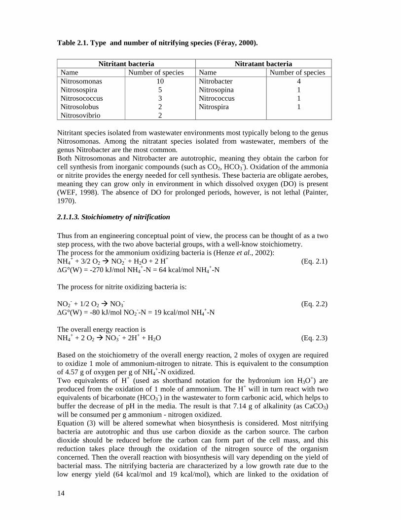
14

Table 2.1. Type and number of nitrifying species (Féray, 2000).

Nitritant bacteria Nitratant bacteria

Name Number of species Name Number of species Nitrosomonas Nitrosospira Nitrosococcus Nitrosolobus Nitrosovibrio

10 5 3 2 2

Nitrobacter Nitrosopina Nitrococcus Nitrospira

4 1 1 1

Nitritant species isolated from wastewater environments most typically belong to the genus Nitrosomonas. Among the nitratant species isolated from wastewater, members of the genus Nitrobacter are the most common. Both Nitrosomonas and Nitrobacter are autotrophic, meaning they obtain the carbon for cell synthesis from inorganic compounds (such as CO2, HCO3

-). Oxidation of the ammonia or nitrite provides the energy needed for cell synthesis. These bacteria are obligate aerobes, meaning they can grow only in environment in which dissolved oxygen (DO) is present (WEF, 1998). The absence of DO for prolonged periods, however, is not lethal (Painter, 1970).

2.1.1.3. Stoichiometry of nitrification Thus from an engineering conceptual point of view, the process can be thought of as a two step process, with the two above bacterial groups, with a well-know stoichiometry. The process for the ammonium oxidizing bacteria is (Henze et al., 2002): NH4

+ + 3/2 O2 � NO2- + H2O + 2 H+ (Eq. 2.1)

∆G°(W) = -270 kJ/mol NH4+-N = 64 kcal/mol NH4

+-N The process for nitrite oxidizing bacteria is: NO2

- + 1/2 O2 � NO3- (Eq. 2.2)

∆G°(W) = -80 kJ/mol NO2--N = 19 kcal/mol NH4

+-N The overall energy reaction is NH4

+ + 2 O2 � NO3- + 2H+ + H2O (Eq. 2.3)

Based on the stoichiometry of the overall energy reaction, 2 moles of oxygen are required to oxidize 1 mole of ammonium-nitrogen to nitrate. This is equivalent to the consumption of 4.57 g of oxygen per g of NH4

+-N oxidized. Two equivalents of H+ (used as shorthand notation for the hydronium ion H3O

+) are produced from the oxidation of 1 mole of ammonium. The H+ will in turn react with two equivalents of bicarbonate (HCO3

-) in the wastewater to form carbonic acid, which helps to buffer the decrease of pH in the media. The result is that 7.14 g of alkalinity (as CaCO3) will be consumed per g ammonium - nitrogen oxidized. Equation (3) will be altered somewhat when biosynthesis is considered. Most nitrifying bacteria are autotrophic and thus use carbon dioxide as the carbon source. The carbon dioxide should be reduced before the carbon can form part of the cell mass, and this reduction takes place through the oxidation of the nitrogen source of the organism concerned. Then the overall reaction with biosynthesis will vary depending on the yield of bacterial mass. The nitrifying bacteria are characterized by a low growth rate due to the low energy yield (64 kcal/mol and 19 kcal/mol), which are linked to the oxidation of

15

ammonium and nitrite, respectively. During nitrification, a major part (80%) of the energy released by the oxidation of the NH4

+ and NO2- is used for CO2 fixing , another part is used

for the cell synthesis (2 to 11 % for Nitrobacter, for example) (Bock et al., 1986) and the remainder is in the form of storage. This explains why the yield constants of nitrification process are small. The maximum yield constant of nitrifying bacteria for the total nitrification process are 0.1 – 0.15 g/g compared with 0.6 - 0.7 g/g of the yield constant of heterotrophic aerobic biomass (Henze et al., 1996; WEF, 1998). In practice, the observed yield, Yobs, is often smaller than maximum yield due to maintenance/endogenous respiration. The equations of ammonium oxidation reaction and nitrite oxidation reaction with the observed yield of ammonium-oxidizers Yobs,NH4 = 0.1 g VSS/g NH4

+-N (= 0.14 g COD/g NH4

+-N) and the observed yield of nitrite-oxidizers Yobs,NO2 = 0.06 g VSS/g NO2--N,

respectively, are written (Henze et al., 2002): 80.7 NH4

+ + 114.55 O2 + 160.4 HCO3- �

C5H7NO2 + 79.7 NO2- + 82.7 H2O + 155.4 H2CO3 (Eq. 2.4)

134.5 NO2

- + NH4+ + 62.25 O2 + HCO3

- + 4H2CO3 � C5H7NO2 + 134.5 NO3

- + 3H2O (Eq. 2.5) The overall equation of reaction for nitrification is found by combining (Eq. 2.4) and (Eq. 2.5). NH4

+ + 1.86 O2 + 1.98 HCO3- �

0.02 C5H7NO2 + 0.98 NO3- + 1.88 H2CO3 + 1.04 H2O (Eq. 2.6)

Compared to the energy reactions (2-1) – (2-3), in the overall equation (Eq. 2.6), the oxygen requirement and alkalinity consumption in nitrification change little when biosynthesis is considered because of the low yield of bacterial mass in the reaction. The oxygen requirement decreases to 4.25 g O2/g NH4

+-N oxidized, whereas alkalinity consumption decreases to 7.07 g as CaCO3/g NH4

+-N used. These differences are due to the fact that inorganic carbon (CO2, HCO3

-), which is assimilated by the bacteria, also acts as an oxidizing agent thus reducing somewhat the oxygen consumption (Henze et al., 2002) and a small part of ammonia used for biomass synthesis does not participate in the reaction with bicarbonate. In design, the values derived from the energy reactions (4.57 g O2 consumed and 7.14 g alkalinity (as CaCO3) consumed per g of NH4

+-N oxidized) typically are usually used (WEF, 1998). The amounts of alkalinity (HCO3

-) consumed in reactions (Eq. 2.4) and (Eq. 2.6) are rather close.

2.1.1.4. Kinetics of nitrification Kinetics of microbial growth and decay can be described by various models, but the most popular one is Monod’s kinetic. Based on this model the Task Group on Mathematical Modelling for Design and Operation of Biological Wastewater Treatment (IWA) has developed the advanced activated sludge models such as ASM1, ASM2, ASM2d, ASM3, etc. However, it should be considered that such models have certain limitations in stability and generalization compared with chemical and physical processes due to concurrent interaction of various factors in the system (Henze et al., 2002; Henze et al., 2000; Metcalf&Eddy, 1991).

16

Kinetic studies typically have demonstrated the growth rate of Nitrosomonas (or first step) to be lower than that of Nitrobacter (or second step). The oxidation of ammonia to nitrite can be considered usually to be the rate-limiting step in the overall nitrification process. Accordingly, nitrification is often modelled as a one-step reaction, carried out by a group of autotrophic bacteria including both ammonia oxidizers and nitrite oxidizers (WEF, 1998). Monod’s equation is typically used to describe the effect of limiting substrates on microbial growth. A limiting substrate is one of the compounds needed for growth that is present at a concentration low enough to affect the growth rate and consequently the rate of substrate removal. Experimentally, it has been found that the effect of a limiting substrate or nutrient can often be defined adequately using the following expression proposed by Monod (Monod, 1949):

+µ=µ

SAmax,A KS

S (Eq. 2.7)

Where µA specific growth rate of (here nitrifying) biomass (d-1); µmax,A maximum specific growth rate of (here nitrifying) biomass (d-1); S substrate concentration (here in mgN/L);

KS substrate haft-saturation coefficient (here in mgN/L); Monod’s expression shows that the constant of saturation KS can be neglected when the concentration of the substrate is sufficiently high (concentrated industrial wastewater, for example) (Henze et al., 2002). In such circumstances, the kinetics of growth of the micro-organisms is described by a zero order expression, that is, if S >> KS: Amax,A µ=µ (Eq. 2.8)

Both ammonium (as substrate) and DO (as electron acceptor) are important factors for nitrification. Either or both can be low enough in concentration to limit the specific growth rate of nitrifying bacteria in wastewater treatment systems (Metcalf&Eddy, 1991; WEF, 1998). Using this approach, the growth rate of nitrifying bacteria can be described by Monod’s expression as shown in (Eq. 2.9).

+

+µ=µ

O,SO

O

NN

NAmax,A KS

S

KS

S (Eq. 2.9)

Where SN ammonium-nitrogen concentration (mgN/L);

KN ammonia-nitrogen haft-saturation coefficient for nitrification (mgN/L); SO DO concentration of bulk mixed liquor or wastewater (mg O2/L); and KS,O oxygen haft-saturation coefficient for nitrification (mg O2/L). In the (Eq. 2.9), there are three kinetic parameters µm, KN and KS,O. Values of KN and KS,O

obtained from experimental research varies in a large range. KS,O have been reported to range from 0,15 - 2,0 mg/l (WEF, 1998). KN have been found to increase with temperature, (Knowles, 1965) proposed a relationship between KN and temperature for Nitrosomonas in river water, which is written:

KN = 0,4. )15(118,0 oTe − (Eq. 2.10) The (Eq. 2.11) is another one that presents the interrelation between KN and temperature (Metcalf&Eddy, 1991). KN = 100.051T-1.156

(Eq. 2.11)

17

The growth rate of nitrifying bacterial cells can be defined by the following relationship.

NN

NAAmax,AAg KS

SXXr

+µ

=µ= (Eq. 2.11)

Where rg the rate of nitrifying bacterial growth (g/Lh) XA nitrifying biomass concentration (g/L) Substrate conversions of nitrifying micro-organisms can be described by a first order reaction in respect to the biomass

)KS(Y

SXr

NNA

NAAmax,S,V +

µ= (Eq. 2.12)

Where rV,S the removal rate for substrate (ammonium-nitrogen or nitrite-nitrogen) (mgN/Lh); YA the maximum nitrifying yield coefficient (mg/mg) The endogenous decay of nitrifying can be calculated as follows: rd = - kdXA (Eq. 2.13) Where rd the rate of endogenous decay (g/Lh) kd endogenous decay coefficient (d-1) Then the net rate of specific growth rate of nitrifying biomass is calculated:

dS

Amax,A kKS

S' −

+µ=µ (Eq. 2.14)

Where µ’A the net rate of specific growth rate of nitrifying biomass (d-1)

2.1.1.5. The influence of the environmental factors on nitrification There are a number of environmental factors influencing the nitrification process. These includes: substrate concentration, temperature, oxygen, pH and toxic substances (Henze et al., 2002; WEF, 1998). However, apart from certain toxic substances to which the nitrifying micro-organisms are very sensitive, we can distinguish mainly physical factors and biological factors. The influence of these two categories of factors is shown by the following generalized model (Eq. 2.14) (Henze et al., 2002). µ = µmax.f(S).f(SO2).f(pH).f(T) (Eq. 2.15) Representative kinetic coefficients for the suspended growth nitrification process are given in the following table.

18

Table 2.2. Typical kinetic coefficients for the suspended growth nitrification process (pure culture values)a (Metcalf&Eddy, 1991).

Value Coefficient Basis Range Typicalb

Nitrosomonas µm d-1 0.3-2.0 0.7 KS NH4

+-N, mg/L 0.2-2.0 0.6 Nitrobacter µm d-1 0.4-3.0 1.0 KS NO2

--N, mg/L 0.2-5.0 1.4 Overall µm d-1 0.3-3.0 1.0 KS NH4

+-N, mg/L 0.2-5.0 1.4 Y NH4

+-N, mgVSS/mg 0.1-0.3 0.2 kd d-1 0.03-0.06 0.05 a Values for nitrifying organisms in activated sludge will be considered lower than the values reported in this table. b Values reported are for 20oC. Temperature dependency The range of the temperatures favorable to nitrification is rather broad. The lower limit would be 5°C (Jones and Hood, 1980; Niquette et al., 1998) whereas the higher limit would be between 40°C and 45°C (Gay, 1983; Henze et al., 2002). The results found in (Focht and Chang, 1975; Painter, 1970) show that nitrifiers can growth in the range of 4-50oC. Anyway nitrifying processes cannot take place at thermophilic temperature (50-60oC) (Henze et al., 2002). The temperature dependency for nitrifying bacteria is usually described by the exponential modification of van’t Hoff equation (Henze et al., 2002):

))20T(exp().C20()T( omaxmax −κµ=µ (Eq. 2.16)

The Expression applies at least in the 10-22oC temperature range. At higher temperatures (30-35oC) the growth rate is constant, between 35 and 40oC, the growth rate starts to decline towards zero (see Figure 2.1).The nitrifying micro-organisms present an optimal temperature ranging between 25 and 36°C (Balmelle et al., 1992; Focht and Chang, 1975; Henze et al., 2002; Painter, 1970). This optimal temperature, often discussed, is justified by a variety of the conditions of culture, stocks and of the nature of the substrate.

19

Figure 2.1. Nitrification as a function of temperature. As opposed to other biological processes in wastewater treatment, thermophilic nitrifying bacteria are unknown (Henze et al., 2002).

A number of expressions that describes the relationship between the maximum specific growth rate of nitrifiers and temperature have been developed. Table 2.3 summarizes values of the maximum specific growth rate of nitrifier reported in the literature. Table 2.3. Nitrification maximum specific growth rates (Randall, 1992).

µnmax (d

-1) Source µnmax vs temperature, oC 10oC 15oC 20oC

(Downing, 1964) (Downing and Hopwood, 1964) (Hultman, 1971) (Barnard, 1975) (Painter and Loveless, 1983) (Beccari et al., 1979) (Hall and Murphy, 1980) (Lawrence and Brown, 1976)

(0.47)e0.098 (T-15)

(0.18)e0.116 (T-20)

(0.50)100.033 (T-20) 0.33(1.127)T-20 (0.18)e0.0729 (T-15)

0.29 0.10 0.23 0.10 0.12

0.47 0.28 0.34 0.28 0.18

0.77 0.32 0.50 0.37 0.26 0.27 0.46 0.50

Reaction rate constant for nitrifying bacteria at 20oC are listed in Table 2.4.

20

Table 2.4. Reaction rate constants for nitrification at 20oC (Henze et al., 2002).

Parameter Symbol Unit Ammonia

oxidation Nitrite oxidation

Global process

Maximum specific growth rate

µmax,A d-1 0.6-0.8 0.6-1.0 0.6-0.8

Saturation constant KS,NH4,A mg NH4-N/L 0.3-0.70 0.8-1.2 0.3-0.7 Saturation constant KS,O2,A mg O2/L

0.5-1.0 0.5-1.5 0.5-1.0 Maximum yield constant

Ymax,A mg VSS/mg NO3

--N formed 0.1-0.12 0.05-0.07 0.15-0.20

Decay constant bA d-1 0.03-0.06 0.03-0.06 0.03-0.06 Temperature constant for µmax,A and bA

κ oC-1 0.08-0.12 0.07-0.10 0.08-0.12

Dissolved oxygen concentration Nitrifiers are more sensitive to low oxygen concentrations than heterothophs. The oxygen dependency for nitrification process can be described by a Monod expression

+µ=µ

O,SO

OAmax,A KS

S (Eq. 2.17)

or in combination with Monod’s expression related to the effect of substrate on nitrifying growth rate (Eq. 2.17) we get a double Monod expression as presented in (Eq. 2.9).

+

+µ=µ

O,SO

O

NN

NAmax,A KS

S

KS

S (Eq. 2.9)

The saturation constants KS,O which have been reported in the range of 0,15 - 2,0 mg/l (WEF, 1998) are rather dispersed values. Nitrification reactions require DO concentrations greater than 1 mg/l in situ (Metcalf&Eddy, 1991). In the activated sludge process designed for carbon oxidation and nitrification dissolved oxygen concentration is often maintained in the range 2-3 g/m3. If either KS,O = 2 mg/l or KS,O = 0,15 mg/l are accepted, DO concentration will be either in excess or deficient, respectively (Le, 2006). The reason of the phenomenon mentioned above relates mostly to structure of the biofloc particle and diffusion-dispersion process of oxygen inside the floc (Eckenfelder, 2000; Le, 2006; WEF, 1998). The oxygen concentration in the mixed liquor is different from that in the particle (biofloc), where organic matter oxidization and nitrification reactions take place. Increasing the oxygen concentration in the reactor will speed up diffusion in the floc particle. However the quantity of oxygen consumed in the floc particle is often higher than that produced by diffusion. In other words, the resistance of the floc particle to the oxygen mass transfer into the floc particle can make the rate of oxygen diffusion the rate-limiting step to the overall nitrification process. The concentration of DO within the floc can be affected by a number of parameters. These are the floc shape and size, mixing intensity, temperature of reaction system, growth rate of the bacteria and bio-chemical reactions within the floc. According to (Hanaki et al., 1990) , the heterotrophic bacteria in a single-sludge system may assimilate ammonia faster than nitrifiers, then reducing the ammonia available for nitrifiers. The heterotrophs may also impede the transport of ammonia and DO within the floc. These findings would help to explain why nitrification is slower in combined systems

21

for carbon and ammonia oxidation than in two stage nitrification processes. This concept is illustrated in Figure 2.2. Regardless of the specific mechanism, the apparent effect of mass-transfer limitations is to increase the haft-saturation coefficient and increase the minimum DO required for nitrification.

Figure 2.2. Illustration of substrate concentration profiles within a microbial floc showing simultaneous nitrification and denitrification (Bakti and Dick, 1992).

pH dependency The nitrification process is pH dependent with an optimum in a relative broad range of 8-9 (Henze et al., 2002) (see Figure 2.3) or 7.5-8.5 (Bock, 1989; WEF, 1998). At pH below 6 or above 10, the nitrification rate approaches zero (WEF, 1998).

Ammonium Nitrate Nitrite Organic Carbon Dissolved Oxygen Radial Distance

Con

cent

ratio

n A

noxi

c Z

one

A

ero

bic

Zon

e

Sta

gna

nt L

aye

r

Floc Center

Floc Surface

Bulk Liquid

22

Figure 2.3. The overall nitrification rate as a function of pH (Henze et al., 2002).

The influence of pH in nitrification has been reported in terms of the ratio of the specific growth rate or activity of a culture at a particular pH to the specific growth rate or activity of the same culture or a parallel culture at the optimum pH. Relationships between this ratio (symbolized as fpH) and pH have been found in a number of studies and are described through expressions as follows:

)pH2.7(083.01fpH −−= (Downing and Hopwood, 1964) (Eq. 2.18)

0.8pH;)110(04.01

1fpH optpHpHopt

=−+

= − (Benefield and Randall, 1980) (Eq. 2.19)

710pH

pH

10x0.5c;10x4.1b;

c

10

10

b1

1fpH −−

−

−

==++

= (Bailey and Ollis, 1986) (Eq. 2.20)

(Eq. 2.18) and (Eq. 2.19) are limited to pH ranges on the left side of the optimum. However, much of the reported data lies above these lines, suggesting that the expressions may be overly conservative, especially considering that most of the data are for unacclimated cultures. (Eq. 2.20) is the Michaelis pH function for the fraction of enzyme in the active state (WEF, 1998). The pH dependency could be linked to the inhibition phenomena of gaseous (free or un-ionized) ammonia (NH3) and un-ionized nitrous acid (HNO2) as we know that these substrates can inhibit Nitrosomonas and Nitrobacter and therefore inhibit both ammonium and nitrite oxidation (Alleman, 1985; Anthonisen et al., 1976; Beccari et al., 1992; Turk and Mavinic, 1986).

23

The uncharged components, NH3 and HNO2 are also known as substrate for nitrifying bacteria (Sharma, 1977). Thus we have a situation where the same component is a substrate whereas, at high concentrations, it can also be an inhibitor. Based on studies of (Anthonisen et al., 1976), (Henze et al., 2002) illustrates the situation in which the equilibrium NH3/NH4

+ and HNO2/NO2 are pH dependent in Figure 2.4 a-c. The pH range in which there is not or very weak inhibition effect on the nitrification process as a function of NH3 and HNO2 is around 5.5-7.3.

Figure 2.4 a. Inhibition of ammonium oxidation with NH3 (0% at 10 g N/m3, 100% at 150 g N/m3) and HNO2 (0 % at 0.2 g N/m3, 100 % at 2.8 g N/m3).

Figure 2.4 b. Inhibition of nitrite oxidation with NH3 (0% at 0.1 g N/m3, 100% at 1 g N/m3) and HNO2 (0% at 0.2 g N/m2, 100% at 2.8 g N/m3).

Figure 2.4 c. Inhibition of the overall nitrificati on process as a function of NH3, HNO2 and pH.

At the same time, it is possible that ammonium and nitrite could inhibit nitrification. Table 2.5 presents the range where the inhibition may get effect.

24

Table 2.5. Ammonium-nitrogen and nitrite-nitrogen concentration range for Nitrobacter inhibition as function of pH (T = 20oC) (Anthonisen et al., 1976; Randall, 1992).

pH NH4

+-N (mg/l) NO2--N (mg/l)

6.0 210 – 2100 30 – 330 6.5 70 – 700 88 – 1050 7.0 20 – 210 260 – 3320 7.5 7 – 70 - 8.0 2 – 20 -

Toxicity dependence As mentioned above, among the two biomasses participating in nitrification, Nitrosomonas has a growth rate which is faster than that of Nitrobacter. Normally, the micro-organisms that have slow growth rate can suffer from environmental conditions more than the micro-organisms which growth faster. Compared with the heterotrophs, the autotrophs has a lower resistance capacity (dozen to some thousands times), they are inhibited partly or completely by a number of toxicants, such as organic matters (phenol compounds, chlorine containing compounds, nitrogen containing compounds…), heavy metals (WEF, 1998). Lethal dose LC-50 for Nitrosomonas of these compounds is relatively low. Table (2.6) presents some examples of LC-50 for Nitrosomonas of some toxic compounds. Table 2.6 LC-50 for Nitrosomonas of some compounds (WEF, 1998)

Toxicant LC-50 Toxicant LC-50 methylen chloride 1.2 mg/l trichloromethylen 0.81 mg/l chloroform 0.48 mg/l 1.3 dichloropropen 0.67 mg/l 1.1.2.2.tetrachloroethan 1.4 mg/l 5 chloro-1 pentyne 0.59 mg/l 2-chloropropionic acid 0.04 mg/l

The effect of some anion on nitrification has been reported in several studies. At concentration of 100 mg fluoride/l, nitrification will be reduced of 80 %. Sulphate at 50 mg/l has no effect. Chloride influences relatively strong on this process, expressing by linear decrease of nitrification when concentration of chloride increases in the range of 40 to 70 mg/l. The rate of nitrification will decrease to 60% when the concentration of this anion reaches some hundred mg/l at pH of 8. Heavy metals at the concentrations of 0.25 mg/l (Ni), 0.25 mg/l (Cr), 0.1 – 0.5 mg/l (Cu) inhibit completely activity capacity of Nitrosomonas. Cyanide is strongly toxic, the efficiency of nitrification reduces to 50 % at the cyanide concentration of 0.1 – 0.2 mg/l and this process will be inhibited completely at cyanide concentration of 0.6 – 0.7 mg/l (WEF, 1998). Concentration in products of nitrification When substrate is not limiting, the nitrifying bacteria can be inhibited by the products of their own biological activity (in particular nitrite and nitrate). These products can inhibit

25

the Nitrosomonas and Nitrobacter with extremely high concentrations (300 - 4000 mg.l-1) (Kouakou, 2007). Hydraulic residence time (HRT) HRT is defined as the relationship between the volume of the reactor and the flow rate of wastewater filled to the reactor (Le, 2006). It is consequently described by the following expression:

Q

VHRT = (Eq. 2.21)

Solid retention time (SRT) SRT is equivalent physically to the existing time (e.g. day) of biomass in the system (only in reaction reactors, but not in other steps such as settling) (Le, 2006). This corresponds analytically to the reciprocal of the growth rate of the micro-organisms, which is presented in (Eq. 2.22)

µ= 1

SRT (Eq. 2.22)

Where µ specific net growth rate of micro-organisms (d-1) Nitrification can be influenced considerably by the sludge age. Indeed, considering the low growth rate of nitrifying bacteria, a high sludge age makes it possible to accumulate the biomass and to support a better nitrification. This is why this criterion is sometimes used as strategy of follow-up of process, leading to the mineralization of sludge (and thus a weak production of sludge). The result of chemostat or activated sludge has showed that, if the 1/SRT is greater than the growth rate of the nitrifying micro-organisms, then the population of nitrifiers will be depleted or flushed from the system. Complete nitrification is typically assured in aerobic reactors if the SRT is greater than 10 days (Kouakou, 2007). But according to (Duchènn et al., 1990), to obtain a nitrification without seasonal limitation, which causes different temperatures, it is necessary to respect an SRT more than or at least equal to 20 days. Type of flocs The size of the flocs is an important parameter which influences the activity of nitrifying bacteria (Tijhuis et al., 1995). An increase in the size of aggregates can simultaneously generate nitrification and denitrification in the same reactor, as no oxygen will diffuse to the center of the larger flocs. According to (Boran et al., 1997), the specific rate of nitrification decrease with the size of the flocs and consequently, a light effect of denitrification could be observed. However, this should be good base for studies on novel ways in nitrification and denitrification that will be discussed in a part of this Chapter.

26

2.1.2. Denitrification

2.1.2.1. Definition Denitrification is the process in which nitrate or nitrite - products of the nitrification is reduced to nitrogen gas. This process is termed anoxic respiration as nitrate or nitrite rather than oxygen is the oxidizing agent (ie the electron acceptor). Denitrification is widespread in nature, it occurs anywhere where nitrate is present, provided that no oxygen (or not too much) is present at the same time (Henze et al., 1995; WEF, 1998). Micro-organisms require nitrogen for protein synthesis with ammonium as a preferred source because this form is used directly in synthesis. However, if no sufficient ammonium is available, some micro-organisms can reduce nitrate to ammonium for this use (Gayle, 1989). This process is referred to as assimilatory nitrate reduction, indicating that nitrogen is incorporated into the cell. It is therefore distinguished from dissimilatory nitrate reduction, which is a respiratory process whereby the micro-organisms obtain energy (WEF, 1998). The denitrification process, also known as dissimilatory nitrate reduction is shown in Figure 2.5. The assimilatory nitrate reduction also presented for the comparison. +5 +3 0 -3 Oxidation level for nitrogen Assimilation NO3

- � NO2

- � [NOH]? � NO2OH � R-NH2

Denitrification NO3

- � NO2- � NO� N2O � N2

-----------------------------------------↑----------------------------------------------------- Nitrification NO3

- NO2- [NOH]? NO2OH NH4

+

Figure 2.5. Reaction sequences for microbiological nitrogen conversions (Henze et al., 2002).

In the denitrification process, nitrite (NO2

-), nitric oxide (NO), and nitrous oxide (N2O) are intermediates. Each step involves a particular reductase enzyme that catalyzes the transfer of electrons to nitrogen. The electron originates from the substrate, that is, the electron donor. Either inorganic (for example, hydrogen or sulfur) or organic waste compounds can serve as substrate for denitrification. As a result of denitrification, the electron donor is oxidized while nitrate is reduced (WEF, 1998).

2.1.2.2. Denitrifying micro-organisms Most denitrifying micro-organisms (denitrifiers) are facultative, meaning they can use either oxygen or nitrate as the terminal electron acceptor in respiration. Many bacteria have the ability to change their metabolism from using oxygen as the final electron acceptor to use nitrate. The electron transport system in a denitrifying organism is identical than the electron transport chain under aerobic conditions, with the exception of the last steps, the nitrate (or nitrite) reductase. The “choice” made by the bacteria of the definitive terminal acceptor depends on the redox potential between the last cytochrome in the electron transport system and oxygen or nitrate. The bacteria prefer oxygen when both oxygen and

27

nitrate are present (Henze et al., 2002). This is because denitrification yields less energy than aerobic respiration (WEF, 1998). Thus, to promote denitrification, oxygen must be excluded. According to studies of (Gayle, 1989), at least 14 bacterial genera are known to contain denitrifying species. They are Bacillus, Pseudomonas, Methanomonas, Paracoccus, Spirillum, and Thiobacillus. Most of the denitrifiers are heterotrophic. It means that the carbon source they use for cell synthesis originates from organic compounds, often the same molecules that are oxidized for energy. There are relatively few species of autotrophic denitrifying bacteria. They obtain carbon for cell synthesis from inorganic compounds. Thiobacillus denitrificant is an example. This organism oxidizes elemental sulfur for energy and obtains carbon for cell biosynthesis from dissolved carbon dioxide or bicarbonate (WEF, 1998).

2.1.2.3. Stoichiometry of denitrification In the biological denitrification, there are four continuous steps occurring with valence (Eq. 2.23) (Grady and Lim, 1980). NO3

- � NO2

- � NO (gas) � N2O (gas) � N2 (gas) (Eq. 2.23) Reaction pathway of denitrification is a rather complex process. However, it can be simplified by the following reaction pathway (Kouakou, 2007). NO3

- + 2H+ + 2e- � NO2- + H2O (Eq. 2.24)

NO2- + 4H+ + 3e- � 0.5N2 + 2 H2O (Eq. 2.25)

NO3- + 6H+ + 5e- � 0.5 N2 + 3 H2O (Eq. 2.26)

Nitrate reduction reactions with methanol, acetic acid and wastewater as organic sources and nitrate as the terminal electron acceptor can be written as in (Eq. 2.27)-(Eq. 2.29) (WEF, 1998). 6NO3

- + 5 CH3OH � 3N2 + 5 CO2 + 7H2O + 6 OH- (Eq. 2.27) 8NO3

- + 5 CH3COOH � 4N2 + 10CO2 + 6 H2O + 8 OH- (Eq. 2.28) 10NO3

- + C10H19O3N � 5N2 + 10CO2 + 3 H2O + NH3 + 10 OH- (Eq. 2.29) The hydroxide ion and carbon dioxide in the water will react with each other to create bicarbonate ions, which are shown in the following stoichiometric equation: OH- + CO2 � HCO3

- (Eq. 2.30)

When organic matter in wastewater is formulized as C18H19O9Nas suggested , then the general equation of denitrification can be written as follows (Henze et al., 2002):

70

1C18H19O9N +

5

1NO3

- + 5

1H+ �

10

1N2 +

70

17CO2 +

70

1HCO3

- + 70

1NH4

+ + 5

1H2O

(Eq. 2.31) ∆Go (W) = -103 kJ/e-eqv = 24,4 kcal/mol (NO3

--N) Simultaneously with denitrification, biosynthesis is taking place, therefore changing the stoichiometry. The overall result is an increase in the electron donor (carbon substrate) required per unit mass of nitrate reduced. The equation of reaction, provided that nitrate is

28

assimilated (with maximum yield constant is 0.36 kg biomass/kg organic matter), is presented in (Eq. 2.32) (Henze et al., 2002). 0.57 C18H19O9N + 3.73 NO3

- + 3.73 H+ � C5H7NO2 + 1.65 N2 + 5.26 CO2 + 3.80 H2O (Eq. 2.32) From the (Eq. 2.32), to reduce 1g NO3

--N, we need 6.09 g organic matter (COD) compared with 2.85 g organic matter (COD) consumed/g NO3

--N reduced in (Eq. 2.31). It could be found that, in denitrification, amount of organic matter used for biosynthesis is more or less double than that used for energy production. Where ammonium is available, the bacteria will always use this as nitrogen source. The reaction of denitrification, provided that ammonium is assimilated (with yield constant of the process around 0.40 kg biomass/kg organic matter), the result is (Henze et al., 2002) 0.52 C18H19O9N + 3.28 NO3

- + 0.48 NH4+ + 2.80 H+

� C5H7NO2 + 1.64 N2 + 4.36 CO2 + 3.8 H2O (Eq. 2.33) This equation of reaction does not differ much from (Eq. 2.32) since the ratio of g organic matter (COD) consumed/g NO3

--N reduced is 6.32. But it should be remembered that the maximum yield constant is changed. The yield constant of denitrification is in the range of 0.46 – 0.69 g COD/g NO3

--N (Le, 2006). Alkalinity production The quantity of alkali produced by denitrification can be calculated from the following balanced (WEF, 1998), when nitrate is used for cell synthesis: NO3

- + 1.08 CH3OH + 0.24 H2CO3 � 0.056 C5H7NO2 + 0.47 N2 + 1.68 H2O + HCO3-

(Eq. 2.34) From (Eq. 2.32), it is found that 4.36 g alkalinity (HCO3

-) is produced per 1 g NO3--N

reduced, corresponding to 3.57 g alkalinity (CaCO3) produced/g NO3--N reduced. In

systems where ammonium is available, the alkalinity production will be reduced by one equivalent per mole of ammonium assimilated (Henze et al., 2002).

2.1.2.4. Kinetics of denitrification The rate of denitrification depends on the type and concentration of compound used as carbon substrate and can be predicted by several mathematical models, including Monod expressions. A higher denitrification can be achieved when soluble readily biodegradable substances are available. Denitrification is essentially zero-order with respect to nitrate or organic matter concentration and first-order with respect to biomass concentration. The rate of denitrification is also strongly affected by the DO concentration, pH, temperature, and reactor configuration. Others vary with the organic loading or solids retention time (Henze et al., 2002; WEF, 1998). These different expressions for denitrification rate (rv,NO) in units of g NO3-N reduced/m3.d or for denitrification rate (rv,x) in units of g NO3-N reduced/g MLSS.d can be expressed as follows:

29

Monod expression (Henze et al., 1986):

h,bgOHO

OH

NONO

NO

SS

SHmax,

H

HNO,v X

KS

K

SK

S

SK

S

Y86.2

Y1r η

+

+

+µ

−= (Eq. 2.35)

Where: rv,NO denitrification rate (mg NO3

- -N/L.d) µmax,H maximum specific growth rate for heterotrophs, (d-1) Xb,h concentration of heterotrophs (mg/L COD) SS concentration of readily degradable organic substrate (mg/L COD) KS haft-saturation coefficient for readily degradable substrate (mg/L COD) SO DO concentration (mg O2/L) KOH haft-saturation for DO in heterotrophic growth (mgO2/L) SNO nitrate concentration (mg N/L) KNO haft-saturation coefficient for nitrate (mg N/L) YH heterotrophic yield (g biomass COD/g substrate COD) Ŋg fraction heterotrops using nitrate for electron acceptor (dimensionless) Zero – order (in respect of nitrate): rv,NO = kX (WEF, 1998) (Eq. 2.36) Where: k empirical rate constant (mg NO3

- - N/mg MLSS.d) X concentration of heterotrophs (mg MLSS/L) The empirical rate expression typically is zero-order with respect to nitrate and first-order with respect to biomass concentration according to (Eq. 2.37) rv = kX (Eq. 2.37) Where: rv rate of denitrification (mg MLSS/mg NO3

--N.d) k empirical rate constant (L/mg NO3

—N.d) X concentration of heterotrophs (mg MLSS/L) When system is provided with external organic matters, represented by ratio F/M or substrates come from endogenous degradation (no external substrate available), the denitrification rate can be expressed through experimental (Eq. 2.37) and (Eq. 2.38) (Refling and Stensel, 1978): When external substrate is available: rv,NO = 0.03 (F:M) + 0.029 (Eq. 2.38) When external substrate is not available rv,NO = 0.12. θc

-0.706 (Eq. 2.39) Where: (F:M) food-to-micro-organisms ratio (g BOD5 applied/g MLSS.d)

30

θc solid retention time (d-1) The values for the biokinetic coefficients for Monod-type expressions are given in Table 2.7. Table 2.7. Reaction rate and stoichiometric constants for denitrification, 20oC (Henze et al., 2002).

Coefficient Symbol Unit Typical range Maximum specific growth rate µmax d-1 3-6 Haft-saturation coefficient, nitrate KS,NO3 gN/m3 0.2-0.5 Haft-saturation coefficient, DO KS,O gO2/m

3 0.1-0.5 Haft-saturation coefficient, COD KS,COD gCOD/m3 10-20 Maximum yield constant, COD YCOD gCOD/gCOD 0.5-0.55 Maximum yield constant, NO3

--N YNO3 gCOD/gNO3-N 1.6-1.8 Decay constant b d-1 0.05-1.0

2.1.2.5. The influence of the environmental factors on denitrification Energy sources (substrate) There are a number of factors influencing substrate consumption in biological denitrification. Three principal factors are given in (WEF, 1998). The first one is the concentrations of the electron acceptors present. These include dissolved oxygen (DO), nitrate (NO3

-), nitrite (NO2-) and sulfate (SO4

2-) which are ranked in priority order used by denitrifiers. In a system, there always exits aerobic heterotrophic as well as denitrifiers who can utilize dissolved oxygen. As mentioned above, these bacteria prefer dissolved oxygen due to high energy production, thus denitrification just can start when most of DO has been reduced. Nitrate and nitrite compete on approximately an equal basis for electrons from substrate. Sulfate is present in varying concentrations in wastewater. It can be used as electron acceptor, but only after almost DO, nitrate and nitrite have been consumed. Thus, denitrification can be obtained nearly completely without sulfate reduction. The second factor is the nature of the molecule of electron donor. Denitrifiers can use a broad spectrum of energy sources. Organic compounds are used as electron source for energy metabolism and as carbon source for cell biosynthesis. Inorganic compounds such as molecular hydrogen and sulfur supply electrons also can be used but for energy metabolism only (catabolim). Among the organic materials, the most interesting are those from organic materials in wastewater and sludge, which is called internal energy sources. Methanol and acetic acid are considered the most interesting among the external carbon and energy sources (Henze et al., 2002). In the case of methanol this is mainly due to the price of this external carbon source. In case of shortage of electron donor, denitrification will not be complete; the quantity of nitrate removed will exceed the quantity of nitrogen produced. In the studies of (Louzeiro et al., 2002) on the influence of methanol as external carbon source on the biological nutrient removal kinetics in a experimental SBR, the denitrification rate (KDN; mgNOx-N/g MLVSS.day) have been reported to increase with increasing methanol concentration (M, mg CH3OH/L) according to the relationship KDN = -0.203M2 + 3.93M. This increase stops

31

when a maximum denitrification rate of ~ 19 mgNOx-N/gMLVSS.day isattained, corresponding to a methanol concentration of ~ 8 mg/L. The third factor is the specific growth rate of denitrifiers. The electron donor requirement for high-growth rate systems will exceed that for low-rate system. Temperature dependency The temperature dependency of the denitrification process is similar to that of the aerobic processes – see (Eq. 2.16). The denitrification process can also take place at 50-60oC, but this range is not much applied in practice. The rate of denitrification is roughly doubled for every 10oC increase in temperature between 5 and 25oC (WEF, 1998) and is approximately 50 % higher than that at 35oC (Henze et al., 2002).. Dissolved oxygen concentration Oxygen that has a direct influence on biokinetics is the oxygen within flocs or biofilms and not in the liquid phase even if DO has to be rather low to avoid diffusion to the center of the floc. In Monod expression, the positive effect of a certain substrate on reaction rate is asymptotic, So/(So + Ko). Oxygen has inhibition effect on the denitrification process, the higher oxygen concentration, the higher inhibition level. Therefore we can use the

following value: O)NO(O,S

)NO(O,S

SK

K

3

3

+−

−

(where KS,O(NO3) is the “saturation constant” for oxygen

inhibition. SO is the oxygen concentration in the liquid phase) to estimate inhibition level on denitrification with a meaning similar to other saturation constants (the rate decreases 50 % at that constant). This value varies depending on the actual condition of the system. In an activated sludge plant, KS,O will be lower than that in a biofilm. In a well mixed - activated sludge plant, this value will decrease by decreasing floc sizes. The same saturation value is frequently used for denitrification, KS,O(NO3), and for aerobic oxidation, KS,O (0,1 – 0,5 mg O2/l) (Henze et al., 2002). This “software switch” helps to modelize the progressive inhibition of the denitrification process by oxygen. pH dependency As other biological processes, the optimal pH for denitrification is in a relatively large range, around 7 to 9 (Henze et al., 2002; WEF, 1998). At pH around 10 and pH around 6, the rate of denitrification decreases drastically but denitrifiers can slowly be adapted to the pH changing if the pH changes are rather slow. At low pH (< 7), the denitrification is not complete and there is an increasing amount of nitric oxides NO2, NO which can poison micro-organism at low concentration (Henze et al., 2002).

32

2.2. PARTIAL NITRIFICATION AND DENITRIFICATION

2.2.1. Some configurations of biological processes applied in partial nitrification/denitrification.

2.2.1.1. Conventional nitrification/denitrification process

As presented in Part 2.1 of this chapter, the conventional nitrogen removal will be a combination of two biological processes in which ammonia is aerobically oxidized to nitrite then to nitrate (nitrification); subsequently, this nitrate is reduced to nitrite and finally to gaseous nitrogen (denitrification). The possible metabolic pathways for nitrification and denitrification are shown in Figure 2.6 NH4

+ � NH2OH � [NOH] � NO2- � NO3

- � NO2- � NO2 � NO � N2

Figure 2.6. The metabolic pathways for conventional nitrification and denitrification

NH4

+ + 1.5O2 � NO2- + H2O + 2 H+ (Eq. 2.1) NO2

- + 0.5 O2 � NO3- (Eq. 2.2)

NH4+ + 2 O2 � NO3

- + 2 H+ + H2O (Eq. 2.3) NO3

- + 2H+ + 2e- � NO2- + H2O (Eq. 2.24)

NO2- + 4H+ + 3e- � 0.5N2 + H2O (Eq. 2.25)

NO3- + 6H+ + 5e- � 0.5 N2 + 3H2O (Eq. 2.26)

6NO3- + 5CH3OH � 3N2 + 5 CO2 + 7H2O + 6OH- (Eq. 2.27)

According to overall nitrification (Eq. 2.3), the complete nitrification reaction consumes a large amount of oxygen, requiring 4.57 g of oxygen for each gram of ammonium oxidized. During denitrification, the requirement for organic carbon is significant. For example, according to (Eq. 2.27), to reduce 1g nitrite, it requires 2.47 g of CH3OH. This is especially costly if C/N ratio of wastewater is low since a large amount of external carbon such as methanol is required to add to the full-scale denitrification system (Khin and Annachhatre, 2004; Mosquera-Corral et al., 2005; Schmidt et al., 2003).

2.2.1.2. Partial nitrification Figure 2.7. Partial nitrification (Schmidt et al., 2003)

Partial nitrification is the oxidation of ammonium to nitrite, but not to nitrate (Schmidt et al., 2003), which is based on the fact that nitrite is an intermediary compound in both steps: nitrification up to nitrite is followed by nitrite denitrification (Ciudad et al., 2005). The process diagram is given in Figure 2.7.

(100) (100) (100)

NH4+

Partial Nitrification

Denitrification NO2- N2

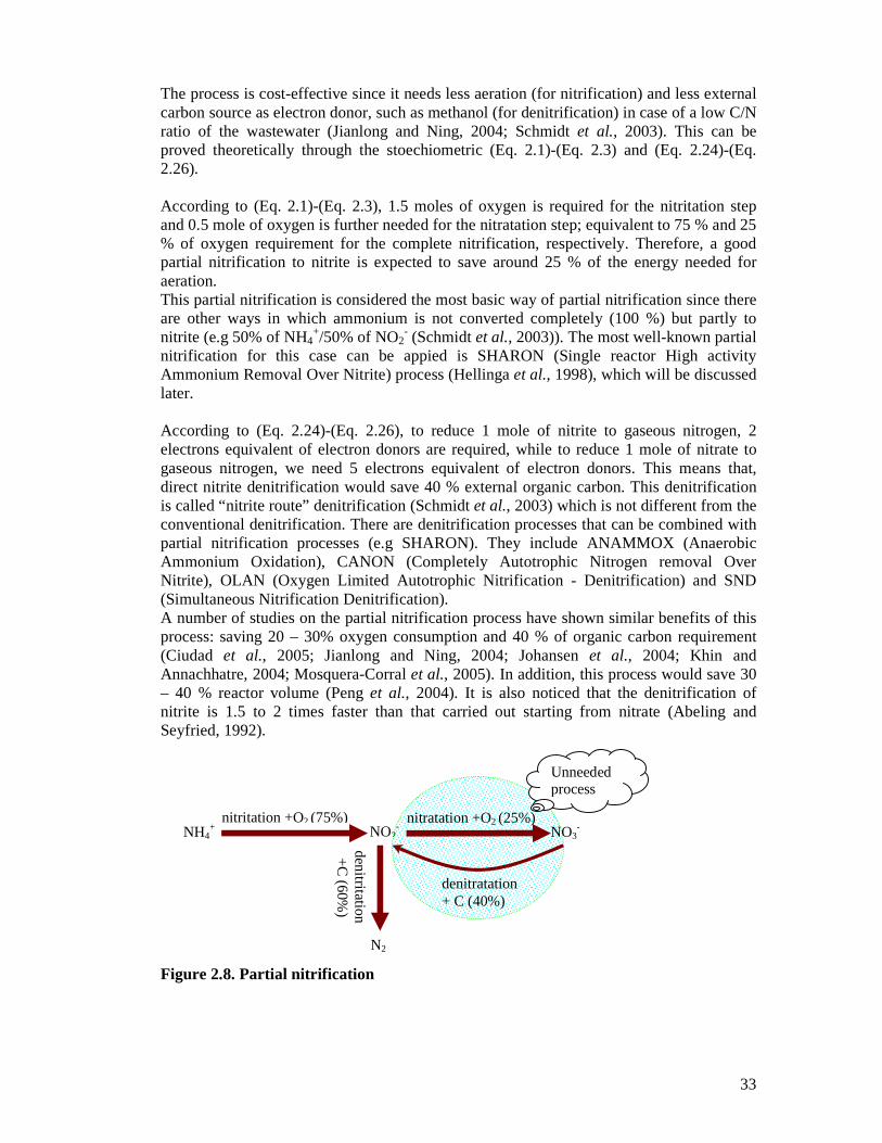
33

The process is cost-effective since it needs less aeration (for nitrification) and less external carbon source as electron donor, such as methanol (for denitrification) in case of a low C/N ratio of the wastewater (Jianlong and Ning, 2004; Schmidt et al., 2003). This can be proved theoretically through the stoechiometric (Eq. 2.1)-(Eq. 2.3) and (Eq. 2.24)-(Eq. 2.26). According to (Eq. 2.1)-(Eq. 2.3), 1.5 moles of oxygen is required for the nitritation step and 0.5 mole of oxygen is further needed for the nitratation step; equivalent to 75 % and 25 % of oxygen requirement for the complete nitrification, respectively. Therefore, a good partial nitrification to nitrite is expected to save around 25 % of the energy needed for aeration. This partial nitrification is considered the most basic way of partial nitrification since there are other ways in which ammonium is not converted completely (100 %) but partly to nitrite (e.g 50% of NH4

+/50% of NO2- (Schmidt et al., 2003)). The most well-known partial

nitrification for this case can be appied is SHARON (Single reactor High activity Ammonium Removal Over Nitrite) process (Hellinga et al., 1998), which will be discussed later. According to (Eq. 2.24)-(Eq. 2.26), to reduce 1 mole of nitrite to gaseous nitrogen, 2 electrons equivalent of electron donors are required, while to reduce 1 mole of nitrate to gaseous nitrogen, we need 5 electrons equivalent of electron donors. This means that, direct nitrite denitrification would save 40 % external organic carbon. This denitrification is called “nitrite route” denitrification (Schmidt et al., 2003) which is not different from the conventional denitrification. There are denitrification processes that can be combined with partial nitrification processes (e.g SHARON). They include ANAMMOX (Anaerobic Ammonium Oxidation), CANON (Completely Autotrophic Nitrogen removal Over Nitrite), OLAN (Oxygen Limited Autotrophic Nitrification - Denitrification) and SND (Simultaneous Nitrification Denitrification). A number of studies on the partial nitrification process have shown similar benefits of this process: saving 20 – 30% oxygen consumption and 40 % of organic carbon requirement (Ciudad et al., 2005; Jianlong and Ning, 2004; Johansen et al., 2004; Khin and Annachhatre, 2004; Mosquera-Corral et al., 2005). In addition, this process would save 30 – 40 % reactor volume (Peng et al., 2004). It is also noticed that the denitrification of nitrite is 1.5 to 2 times faster than that carried out starting from nitrate (Abeling and Seyfried, 1992). Figure 2.8. Partial nitrification

nitritation +O2 (75%)

denitritation

+

C (60%

)

NH4+ NO2

- NO3-

denitratation + C (40%)

N2

nitratation +O2 (25%)

Unneeded process

34

2.2.1.3. SHARON (Single reactor High activity Ammonia Removal Over Nitrite) process The SHARON process involves partial nitrification of ammonium to nitrite to get as much as possible nitrite as the main product of nitrification with some strictly controlled conditions. SHARON is the first successful process in which nitrification/denitrification with nitrite as an intermediate has been achieved under stable conditions (van Kempen et al., 2001). The process operated without any biomass retention is controlled by hydraulic residence time of the system, generally about 1 day (van Dongen et al., 2001) in a single aerated reactor at a relatively high temperature (35 oC or at least above 25 oC) and pH (above 7) (Brouwer et al., 1996; Hellinga et al., 1998). The mechanism of operation of the SHARON process is based on the difference between the growth kinetics of the nitritant micro-organisms (e.g Nitrosomonas) and nitratants (e.g Nitrobacter) (Hellinga et al., 1998; Schmidt et al., 2003). Under these optimal conditions, it supports the growth of the nitritants while washing out the nitratants. The SHARON process can be carried out in a simple continuous stirred tank reactor and is ideally suited to remove nitrogen from waste stream with a high ammonium concentration (> 0.5 g N/l) (Hellinga et al., 1998; Jetten et al., 1997; van Dongen et al., 2001). With the SHARON process, a nitrogen removal efficiency of 85 – 90 % can be achieved (Hellinga et al., 1998; Mulder and Hellinga, 2001; van Kempen et al., 2001) and can save 25 % of aeration energy and 40 % of carbon source addition cost (Hellinga et al., 1998; van Dongen et al., 2001). The full-scale experience has recently been obtained during its operation (Mulder and Hellinga, 2001; van Kempen et al., 2001). The process requires relatively little initial investment because a simple well-mixed tank reactor of modest dimensions without sludge retention is sufficient (Hellinga et al., 1998). The process does not produce chemical sludge and has a relatively low production of biological sludge (Khin and Annachhatre, 2004). In the study of (Schmidt et al., 2003), this process is combined to ANAMMOX process, therefore it is modified to produce a certain ratio of ammonium/nitrite (e.g. 50/50). Figure 2.9. SHARON process (Schmidt et al., 2003).

The most well-known micro-organisms that carries out the SHARON process is Nitrosomonas eutropha (Logemann et al., 1998). This belongs to genera Nitrosomonas of the beta-ammonia oxidizers (Bateman, 1997). To obtain a stable partial nitrification, the oxidation of nitrite to nitrate must be prevented, allowing the accumulation of nitrite in the system. A number of operating parameters (e.g. dissolved oxygen, pH, temperature, hydraulic residence time, solid retention time, substrate concentration) have been studied in chemostat reactors based on influence in the growth rate of nitrifiers (particularly nitrosomonas and nitrobacter) (Beccari et al., 1979; Hellinga et al., 1998; Mosquera-Corral et al., 2005). For instance, to provide a 50 % ammonium oxidation, ammonium and bicarbonate should be present in a molar ratio of 1:1(Mulder et al., 1995). The effect of these parameters on the process will be discussed later in the part “Working condition for partial nitrification/denitrification”.

NH4+

SHARON Anammox NH4+/ NO2

-

(100) (50/50)

35

2.2.1.4. ANAMMOX (Anaerobic Ammonium Oxidation) process The ANAMMOX process is the denitrification of nitrite to produce dinitrogen gas with ammonium as the electron donor under anoxic or oxygen-limited conditions (Jetten et al., 1999; Jianlong and Jing, 2005; Kuai and Verstraete, 1998; Mulder et al., 1995; Schmidt et al., 2003) by autotrophic micro-organisms without addition of external carbon source (Jetten et al., 2005; Jetten et al., 1999). It is suggested that nitrate could also be used as an electron acceptors in the ANAMMOX reaction but only after the exhaustion of nitrite (Jianlong and Jing, 2005). In other words, nitrite is the preferred electron acceptor for the process (Bock et al., 1995; Van de Graaf et al., 1995). This is possibly due to higher energy production in the reaction with nitrite as electron acceptor, as shown in the (Eq. 2.40) and (Eq. 2.41). According to (Van de Graaf et al., 1995), at the beginning of the reaction, ammonium directly reacts with nitrite to produce dinitrogen gas, which is given in the (Eq. 2.40). NH4

+ + NO2- � N2 + 2 H2O (Eq. 2.40)

G’O = - 358 kJ/mol NH4+

(Mulder et al., 1995) suggested that ammonium oxidation can couple to nitrate reduction in a smaller fluidized denitrification reactor. The stoichiometric reaction can be hypothesized as in (Eq. 2.41). 5 NH4

+ + 3 NO3- � 4 N2 + 9 H2O + 2 H+

(Eq. 2.41) G’O = - 297 kJ/mol NH4

+ In the ANAMMOX process with nitrite as electron acceptor, the main product is dinitrogen gas, but about 10 % of nitrite and ammonium are converted into nitrate (Khin and Annachhatre, 2004). (Strous et al., 1998) determined the stoichiometry based on mass balance over ANAMMOX enrichment cultures of the combined catabolic and anabolic reactions as given in (Eq. 2.42). NH4

+ + 1.32 NO2- + 0.066 HCO3

- + 0.13 H+ � 1.02 N2 + 0.26 NO3

- + 0.066 CH2O0.5N0.15 + 2.03 H2O (Eq. 2.42)

Figure 2.10 ANAMMOX process (Schmidt et al., 2003).

The ANAMMOX needs a preceding partial nitrification step, that converts around 50 % of the wastewater ammonium to nitrite (Dapena-Mora et al., 2004; Schmidt et al., 2003). The combination between ANAMMOX and SHARON process with an appropriate ammonium/nitrite ratio have been applied successfully in the laboratory (van Dongen et al., 2001; Van Loosdrecht and Jetten, 1997; Volcke et al., 2005). By simply not supplying any carbon source (e.g. methanol) and removing the oxic periods or by limiting the oxygen

NH4+/NO2

- ANAMMOX N2/NO3

-

(50/50) (90/10) SHARON

36

supply to a nitrification reactor with sludge retention, a SHARON reactor yields the desired ammonium/nitrite mixture. This is possible because when 50 % of the ammonium is oxidized, the decrease in pH (to 6.7) prevents the oxidation of the remaining ammonium (Schmidt et al., 2003; Strous et al., 1997). This process allows over 50 % of the oxygen to be saved and no organic carbon source is needed (Van de Graaf et al., 1996). In addition, the biomass yield is very low so that little sludge is produced (Jetten et al., 1997; Jianlong and Jing, 2005). ANAMMOX process is carried out by a group of planctomycete bacteria (Strous et al., 1999a). The most two common ANAMMOX bacteria that have been tentatively named ‘‘ Candidatus Brocadia anammoxidans’’ (Jetten et al., 2001; Strous et al., 1999a) and ‘‘ Canidatus Kuenenia stuttgartiensis’’ (Schmid et al., 2000). The former is a chemolithoautotrophe, having a doubling time of 11 days and a biomass yield of 0.13 g VSS/g NH3-N (Strous et al., 1998). Like ammonium oxidizers, these bacteria have a very high affinity for the oxygen, ammonia (as a substrate) and nitrite (as an inhibitor). It is irreversibly inhibited by nitrite at concentrations in excess of 70 mg N/l for several days and by phosphate at concentration above 60 mg P/l for several days (Strous et al., 1999b; Strous et al., 1997; Van de Graaf et al., 1996). The later has a higher tolerance to nitrite (180 mg N/l), is more active in low cell density cultures and is less inhibited by phosphate (600 mg P/l) (Egli et al., 2001). The ANAMMOX process is seven times slower than aerobic ammonium oxidation (Strous et al., 1998) but ANAMMOX bacterial activity is 25-fold higher than aerobic ammonium oxidizers under anoxic conditions when using nitrite as the electron acceptor (Jetten et al., 1999). Oxygen concentration as low as 2 µM inhibits the ANAMMOX activity completely but reversibly (Jetten et al., 2001). Together with ammonia as a substrate, carbon dioxide is the main carbon source for the growth of ANAMMOX bacteria (Van de Graaf et al., 1996). At laboratory scale, ANAMMOX process has been tested and show their suitability in several kinds of reactor, such as fluidized bed (Van de Graaf et al., 1996), fixed bed (Strous et al., 1997), sequencing batch reactor and gas-lift reactor (Dapena-Mora et al., 2004; Strous et al., 1998). Concerning the ANAMMOX process, one of the main challenges is long start-up time due to very slow growth of the ANAMMOX planctomycetes. It takes from 100 to 150 days before an ANAMMOX reactor inoculated with activated sludge reaches full capacity (Schmidt et al., 2003; van Dongen et al., 2001).

Table 2.8 presents some stoichiomestric and kinetic parameters of Anammox micro-organisms in comparation with nitrite nitrifying mi rcro-organisms (nitritant).

Parameters Unit Nitritant Anammox Note Source Biomass yield Y

Mol/mol C 0.08 0.07

Aerobic rate Nmol/min/mg protein

200-600 0

Anaerobic rate Nmol/min/mg protein

2 60

Growth rate h-1 0.04 0.003 Doubling rate Day 0.73 10.6 KsNH4

+ µM 5-2600 5 KsNO2

- µM N/A <5

KsO2 µM 10-50 N/A

(Jetten et al., 2001) Parameters of aerobic and anaerobic ammonia oxidation. N/A: not applicable; Ks: affinity constant.

37

Aerobic ammonium oxidisers (XNH) maxNHµ h-1 0.8

bNH h-1 0.05

1/K = 0.094

Aerobic nitrite oxidisers (XNO) maxNOµ h-1 0.79

bNO h-1 0.033

1/K = 0.061

Anaerobic ammonium oxidisers ANAMMOX (XAN) maxANµ h-1 0.028

bAN h-1 0.001

1/K = 0.096

(Hao et al., 2002) Growth rates and endogenous respiration rates and their temperature dependency (1/K) for nitritification, nitratification and ANAMMOX at 20oC.

2.2.1.5. CANON (Completely Autotrophic Nitrogen Removal Over Nitrite) Process CANON process is the combination of partial nitrification and ANAMMOX in a single, aerated reactor (Strous et al., 1997; Third et al., 2001). This process removes ammonium from wastewater with high ammonium loading and containing low amounts of organic matters (Dijkman and Strous, 1999; Helmer et al., 2001; Kuai and Verstraete, 1998; Siegrist et al., 1998). According to (Strous, 2000), the process relies on the interaction of two groups of autotrophic aerobic and anaerobic ammonium-oxidizing bacteria under oxygen-limiting conditions that perform two sequential reactions, simultaneously. Under oxygen limitation (< 0.5 % air saturation), ammonium is oxidized to nitrite by aerobic ammonium oxidizers, such as Nitrosomonas and Nitrosospira (Third et al., 2001), which is shown in (Eq. 2.1) (Hanaki et al., 1990). NH4

+ + 1.5 O2 � NO2- + H2O + 2H+ (Eq. 2.1)

Subsequently, anaerobic ammonium-oxidizing bacteria like Planctomycete (Third et al., 2001) convert ammonium with the produced nitrite to dinitrogen gas and small amounts of nitrate, which is given in (Eq. 2.43) (Strous, 2000). NH4

+ + 1.3 NO2- � 1.02 N2 + 0.26 NO3

- + 2 H2O (Eq. 2.43) The overall stoichiometric reaction that combine the above two reactions (Eq. 2.1) and (Eq. 2.32) can be expressed as in (Eq. 2.44) (Strous, 2000). NH4

+ + 0.85 O2 � 0.435 N2 + 0.13 NO3- + 1.3 H2O + 1.4 H+ (Eq. 2.44)

Because the CANON process is completely autotrophic, it avoids the external carbon addition often required for heterotrophic denitrification step in the conventional systems. In addition, the entire nitrogen removal can be achieved in a single reactor with very low aeration, greatly reducing space and energy requirement (63 % less oxygen consumption and 100 % less electron donor than traditional systems) (Third et al., 2001). In studies with a sequencing batch reactor and a gas lift reactor, nitrogen removal rate was up to 0.3 and 1.5 kg N total m-3 day–1, respectively, have been reported for the CANON process (Sliekers et al., 2002; Sliekers et al., 2003). CANON needs process control to prevent nitrite build-up by oxygen excess (Schmidt et al., 2003).

38

2.2.1.6. SND (Simultaneous Nitrification Denitrification) Process SND, as it names, implies that nitrification and denitrification occur concurrently in the same reactor under identical overall operating conditions (Beun et al., 2001; Munch et al., 1996). This process has been observed in several studies (Ho, 1994; Kokufuta et al., 1988; Masuda et al., 1991). SND offers the potential to save the cost for a second (anoxic) tank, or at least reduce its size, if it can be ensured that a considerable amount of denitrification takes place together with nitrification in the aeration tank. (Turk and Mavinic, 1986; Turk and Mavinic, 1989) reported some advantages of SND process such as a 40 % reduction of COD required for denitrification, 63 % higher denitrification rates. The given explanations for the phenomenon of SND can be divided into broad categories, physically and biologically (Munch et al., 1996). Physically, SND occurs as a consequence of DO concentration gradients within microbial flocs or biofilms due to diffusional limitations. That is, the nitrifiers exist in regions with high dissolved oxygen concentrations, whereas the denitrifiers will preferentially be active in zones with very low dissolved oxygen concentrations. Biologically, SND can occur since there is existence of aerobic denitrifiers as well as heterotrophic nitrifiers, and nitrification under fully anaerobic conditions is possible. About 65 % of the ammonium load is converted to nitrite (Ruiz et al., 2006). The effectiveness of these reactors requires to take into account three principal factors: dissolved oxygen concentration, size of the flocs and concentration in organic substrate (Pochana and Keller, 1999). The rate of nitrification and elimination of nitrogen reported by several studies is up to 90 % and 93 %, respectively (Ruiz et al., 2006; Yoo et al., 1999). This process should be distinguished from NOx process which was proposed by (Schmidt et al., 2003). The NOx is processes in which, in the presence of NOx, Nitrosomonas-like micro-organisms nitrify ammonium and denitrify nitrite produced simultaneously even under fully oxic condition to dinitrogen gas as the main product (Figure. 2.11). Figure 2.11 NOx process

* In the presence of oxygen the supplemented NOx (NO/NO2) is the regulatory signal including the denitrification activity of the ammonia oxidizers and it is only added in trace amount (NH4

+/NO2 above 1000/1 to 5000/1) (Schmidt et al., 2003).

NH4+/NO2

- Denitrification N2

(60/40) (100) NOx

Process

NH4+/NO2

(1000/1*)

39

2.2.2. Operating conditions for partial nitrificati on Resulting from the analysis of the various strategies and configurations mentioned above, the partial nitrification through the nitrite accumulation could be obtained by controlling principle operating parameters (temperature, pH, dissolved oxygen concentration, NH3 concentrations and HNO2, hydraulic residence time, solid retention time, mode of aeration (prolonged and/or intermittent), combination of processes (e.g SHARON-ANAMMOX) etc.). Taking into account these strategies makes it possible to eliminate nitrogen at a reduced cost.

2.2.2.1. Dissolved Oxygen Working conditions for an optimum partial nitrification have been reported in several studies. The first parameter that must be mentioned is dissolved oxygen. The nitratants have a lower affinity for oxygen than the nitritants. This can be explained by previous studies showing that the half-saturation coefficient for dissolved oxygen of Nitrobacter (0.72 – 1.84 mg/l) is higher than that of Nitrosomonas (0.25 – 0.5 mg/l) (WEF, 1998). Therefore, a low dissolved oxygen is restrictive for the growth of nitratants and then hinders the nitratation (Alleman, 1985; Hanaki et al., 1990; Turk and Mavinic, 1989). Oxygen affinity constant for ammonium oxidizers (KO,AOB) was assessed in two different systems in the study of (Galí et al., 2007) who showed values which belong to the known range of (Henze et al., 2002): SBR (at 30oC): 0.34 ± 0.07 mgO2/L and SHARON chemostat reactor (at 35oC): 0.49 ± 0.06 mgO2/L. (Ruiz et al., 2002) studied the influence of different DO on nitritation reporting that, DO in the range of 2.7 – 5.7 mg/l does not influence nitrification. At DO of 1.7 mg/l, there is a temporal nitrite accumulation; and at DO of 1.4 this accumulation increases with an unchanged ammonium consumption rate. Maximum nitrite accumulation is obtained at DO of 0.7 mg/l. At DO of 0.5 mg/l, ammonium accumulation takes place. Depending on the aerobic retention time, different ammonium removal efficiency are achieved in the effluent (van Kempen et al., 2001). The sensitivity of the Anammox enrichment culture to oxygen was investigated under various sub-oxic conditions by (Jetten et al., 1999). In four consecutive experiments, the oxygen tension was decreased stepwise from 2 to 0 % of air saturation. No ammonium was oxidized in the presence of 0.5, 1, or 2 % of air. Only when all the air was removed from the reactor by vigorously pushing with argon gas, the conversion of ammonium and nitrite resumed, thus indicating that the ANAMMOX activity in these enrichment cultures is only possible under strict anoxic conditions. The optimal concentrations of DO for partial nitrification/denitrification reported in several studies on synthetic wastewater are given in the Table 2.8. In addition, (Çeçen and Gönenç, 1994) revealed that the accumulation of nitrite is possible if the ratio dissolved oxygen (DO, in mgO2.l

-1)/free ammonia (FA, in mg NH3l-1 ) satisfies

the relation (Eq. 2.45).

5FA

DO < (Eq. 2.45)

When this relation is respected, the formation of nitrate is inhibited. (Bernet et al., 2005) observed the same phenomenon, suggesting that the dissolved oxygen concentration should not be regarded as being an exclusive variable of control of the accumulation of

40

nitrite. Indeed, this one could also depend on the ammonium load applied, by respecting the relation in (Eq. 2.46)

3.0NHN

DO

4

<− + (Eq. 2.46)

In addition to the possibility of accumulating nitrite in the presence of a low oxygen concentration, the mode of aeration and sludge age also should be considered. The study on the influence of the aeration and the sludge age on partial nitrification carried out by (Pollice et al., 2002), shows that this process is realizable even when oxygen is not limiting (for example in prolonged aeration). With this intention, the residence time of the biomass was tiny kept at 10 days in the system. However, when aeration was reduced (in particular in intermittent aeration), the conversion of ammonium into nitrite was stabilized and this, independently of the sludge retention time in the system. One can deduce from the way in which the strategy of alternative aeration supports the stability of the partial nitrification process (Kouakou, 2007).

2.2.2.2. Temperature As far as we know, there is a difference in activation energy between ammonium and nitrite oxidation processes (64 kcal/mol NH4

+-N and 19 kcal/mol NH4+-N respectively).

The high activation energy of ammonium oxidation makes the rate of this process more dependent on temperature (Schmidt et al., 2003). In the SHARON process, nitritation process can be obtained at high temperature (30 - 40 oC) and temperature at 35 oC was chosen to maintain stable operation. High temperature is favourable condition for nitritation. Nitrite oxidizers growth faster than ammonium oxidizers at normal process in the treatment plant (5 – 20 oC), but the contrary is observed at high temperature (Hellinga et al., 1998). The studies of (Hunik, 1993) have reported that the growth rate of nitritants is higher than that of nitratants at elevated temperatures (15 oC) and at 35 oC, maximum specific growth rate of nitritants is approximately half that of nitratants (0.5 d-1 and 1 d-1, respectively). However, only at temperature above 25 oC, the nitritants can effectively outcompete the nitratants (Brouwer et al., 1996). The ANAMMOX bacteria were found to be active at temperature between 20 oC and 43 oC (with optimum at 37 oC) (Strous et al., 1999b). (Fux et al., 2002) maintained a constant temperature at 30 oC ± 0.7 in ANAMMOX process. For the performance of the CANON process, (Hao et al., 2002) worked at a temperature of 20 oC .

2.2.2.3. Hydraulic retention time (HRT) and Solid residence time (SRT) The SHARON process works without solid residence, meaning that solid residence time (SRT) is controlled by hydraulic retention time (HRT). Thus nitratants are not able to remain in the SHARON reactor and they are washed out as in the chemostat. A hydraulic retention time therefore is selected to be higher than the growth rate of nitritants but lower than that of nitratants (about 1 day) (Hellinga et al., 1998). Because there is no sludge retention and the hydraulic retention time is fixed, the volumetric ammonium reactor loading depends on ammonium concentration (Schmidt et al., 2003).

41

2.2.2.4. pH, alkalinity and NH3/HNO2 As mentioned above, the influence of pH on nitrification process has been studied in detail. In the SHARON process, this parameter turned out to be very important (Hellinga et al., 1998). During nitrification, the pH will decrease significantly (2 mol H+ produced/mol NH4

+oxidized). Approximately 50 % of these H+ will be compensated by bicarbonate formed from denitrification with organic carbon source (e.g methanol) or OH- from base addition. The 50 % remaining H+ will be neutralised by stripping CO2 formed from HCO3

- that is present in the reactor. Due to this proton production/consumption, the pH varies about one pH unit in one nitrification/denitrification cycle (Hellinga et al., 1998). In the study of (Jetten et al., 2001), it is showed that the ammonium : nitrite ratio (1:1) in the effluent of the SHARON process could be fine-tuned by adjusting the pH between 6.5 and 7.5. The effluent of this SHARON reactor was fed to an ANAMMOX SBR and then this reactor removed all nitrite and left some ammonium. The pH influences the formation of free ammonia (NH3 or “FA”) and consequently ammonium (NH4

+). The (Eq. 2.47) presents the balance of couple NH3/NH4+ in which

NH4+ is moved towards NH3 with at high pH values (Metcalf&Eddy, 1991) (see more in

2.1.1.5, in pH dependency). NH4

+ ⇔ NH3 + H+ (Eq. 2.47) (pH = 9.3) The concentration of FA is generally estimated either by the (Eq. 2.48) (Anthonisen et al., 1976), or by (Eq. 2.49) (Verstraete and van Vaerenberg, 1985).

wbpH

pH3

k/k10*14

10NHN17FA

+−

= (Eq. 2.48)

)T0241.0ln(10*398.310

10

)NHNH(

NH9pH

pH

43

3

−=

+∑ + (Eq. 2.49)

Where N-NH3 Total concentration of ammonia, mg NH3-N/l T Temperature, oC kb/kw = e6344/(273+T) The constant ratio of ionization of the couple NH4

+/NH3 and water The accumulation of nitrite is strongly influenced by the pH value or concentration of FA. (Ruiz et al., 2002) reported that at pH < 6.45 or pH > 8.95, the oxidation of ammonia is completely inhibited. In the range 6.45 to 8.95, complete nitrification can be observed with a temporal accumulation of nitrite at pH of 8.65 – 8.95. Complete nitrification is possibly due to the acclimatization of Nitrobacter species to increased concentrations of FA. Whereas in general a small quantity of FA (3.5 mg NH3.l

-

1) is enough to inhibit a non acclimatized biomass, (Turk and Mavinic, 1986) reported that high concentrations (40 mg NH3.l

-1) do not affect an acclimatized biomass. This phenomenon makes that the pH remains an operational variable maybe less interesting to handle in partial nitrification (Ruiz et al., 2002) although it is possible to control it to accumulate nitrite.

42

Since the pH variation relates to NH4+/NH3 and NO2

-/HNO2 ratios, pH has a great influence on the growth of nitratants and nitritants, respectively, as well as their activity in nitratation and nitritation. For nitritants, NH3 is the actual substrate rather than NH4

+ and HNO2- is the inhibitor,

while HNO2- is substrate and NH3 is the inhibitor for nitratants (Anthonisen et al., 1976;

Turk and Mavinic, 1986). (Hellinga et al., 1998) suggested an equation to express the specific growth rate for ammonium oxidizers:

22,

2,

22

2

33

3max

HNOamm

HNOI

ammHNOI

OammO

O

NHammNH

NHammamm

CK

K

CK

C

CK

C

+⋅

+⋅

+⋅= µµ (Eq. 2.50)

The nitratants are inhibited by NH3 even stronger than the inhibition level of HNO2

- for nitritants since nitritants can better tolerate high nitrite concentration (Jetten et al., 1997; van Dongen et al., 2001; WEF, 1998). Thus, for the growth rate of nitrite oxidizers, the equation can be expressed in the same way:

33,

3,

22

2

22

2max

NHnit

NHI

nitNHI

OnitO

O

HNOnitHNO

HNOnitnit

CK

K

CK

C

CK

C

+⋅

+⋅

+⋅= µµ (Eq. 2.51)

amm

3NHK was found close to 7 mgNH3-N/l equaling 0.5 mg NH4+/l at the pH range 6.5-8.5 at

30 oC (Brouwer et al., 1996). The amm2HNO,IK was found 0.2 mg HNO2/l at pH 7 (Hellinga et

al., 1998). It was observed that at low concentration of ammonia (1-5 mg NH3-N.l-1) (Abeling and Seyfried, 1992) or even much lower (about 0.1 – 1 mg NH3-N.l-1) (Anthonisen et al., 1976; Turk and Mavinic, 1986), the nitratation was inhibited. The nitritation was inhibited at concentrations of 5 to 20 mg NH3-N.l-1 (Turk and Mavinic, 1986). This could be an advantage for nitrite accumulation. At an extremely high concentration of ammonia (10 – 150 mg NH3-N.l-1), the total process of the ammonium oxidation can be completely inhibited and any possibility of accumulation of nitrite becomes impossible (Anthonisen et al., 1976). In contrast, the results obtained during the study of (Beline et al., 2007) indicated no inhibition of ammonia nitrifers or nitrite nitrifiers with free [NH3] up to 50 mgN/L. For the ANAMMOX activity, it is found that the process is detectable for both bacteria in a pH range between 6.4 and 8.3 (with optimum at 8) (Egli et al., 2001; Jetten et al., 1999).

43

Table 2.9. Operation condition for partial nitrific ation/denitrification in some studies

Wastewater (Reactor)

Partial nitrifica-tion (PN) process

DO (mg/l)

pH To

(oC) Nitrite accumu-lation (%)

Ammonia /nitrogen/nitrite removal (%)

Source

Synthetic wastewater (SBR)

PN 1.5 7.5 30 - 85 (Jianlong and Ning, 2004)

Synthetic wastewater (AS reactor)

PN 1.4 7.8 25 75 95 (Ciudad et al., 2005)

Simulated industrial wastewater (AS reactor)

PN 0.7 – 1.4

6.45-8.95

- > 65 98 (Ruiz et al., 2002)

Synthetic wastewater (SBR)

PN 2-3 7.45-7.6

95 (Pambrun et al., 2004)

Aminoplastic Resin wastewater (AS reactor)

PN 0.76 23.1 88.6 (Fernández et al., 2005)

Piggery wastewater (SBR)

PN < 0.5 8.0-8.7 > 25 (Beline et al., 2007))

Synthetic wastewater (Biofilm)

PN 1.2 30 71 (Hui-Ping Chuanga et al., 2007)

Synthetic wastewater (SBRDR)

PN 0.8-1.0 7.5-8.6 20 84-88 (Antileo et al., 2006)

membrane Bioreactor

PN 2 8.2 30 (Kouakou, 2007)

Anaerobic sludge reject water (SBR)

PN >3 6.5-8 30 ± 0.5

50

(Galí et al., 2007)

Domestic WW (Chemostat reactor)

SHARON > 8 30-34

90 (Kempen and Mulder, 2001)

Centrifuged sludge digestion effluent (CTTR)

SHARON 7-8 30-40

80-85 (Hellinga et al., 1998)

Anaerobic sludge reject water (Chemostat reactor)

SHARON >2 6.5-6.7 35 ± 0.5

50 (Galí et al., 2007)

Rejection water from dewatering of digested sludge (WWTP)

SHARON 7-8 30 – 40

90 (van Kempen et al., 2001)

Sludge digestor effluent (SHARON reactor/SBR)

SHARON/ANAMMOX

6.5-7.5 53 (Jetten et al., 2001)

Sludge digestion effluent (Fluidized bed reactor)

ANAMMOX

7.7-8.2 30 82 (Strous et al., 1997)

Sludge digestor effluent (Fluidized bed reactor)

ANAMMOX

7.0-8.5 30-37

(Jetten et al., 2001)

44

Synthetic wastewater (Gas-lift)

ANAMMOX

8. ± 0.1 30 88/99 (Dapena-Mora et al., 2004)

Synthetic wastewater (SBR)

ANAMMOX

7.8-8.0 35 78/99 (Dapena-Mora et al., 2004)

Sludge digestor effuent (SBR)

ANNAMOX

7-8 30-37

(Jetten et al., 2005)

Domestic wastewater (SBR)

CANON 2.7 7.78 28.7 58 92 (Fux et al., 2002)

Synthetic wastewater (Biofilm)

CANON 0.8 30 74 (Hao et al., 2002)

Synthetic wastewater (SBR)

CANON < 0.3 7.8 30 85 (Sliekers et al., 2002)

Synthetic wastewater (SBR)

CANON <1 7.8 30 (Third et al., 2005b)

Domestic wastewater (SBR)

SND 0.2 75 (Holman and Wareham, 2005)

Industrial wastewater (SBR)

SND 1 75 (Holman and Wareham, 2005)

Synthetic wastewater (SBR)

SND 0.64-0.68

25±2

98.7 (Chiu et al., 2007)

Synthetic wastewater (SBR)

SND 1 25 52 (Third et al., 2005a)

Synthetic wastewater (IDEA)

SND 0.3-1.0 22-27

90 (Yoo et al., 1999)

Domestic wastewater (SBR)

SND 0.5 18-22

98 (Munch et al., 1996)

Artificial wastewater (AS pilot)

SND 7.2-8.3 25-30

96 (Dahl et al., 1997)

Slaughterhouse wastewater (SBR)

SND < 0.8 7-8 18-22

95 (Pochana and Keller, 1999)

Note: AS: Activated sludge CSTR: Continuously stirred tank reactor IDEA: intermittently aerated and decanted single-reactor SBR: Sequencing batch reactor SBRDR: Sequencing batch rotating ditch reactor

45

REFERENCE

1. Abeling, U., and C. F. Seyfried, 1992, Anaerobic-aerobic treatment of high strength ammonium wastewater nitrogen removal via nitrite: Water Science and Technology, v. 26, p. 1007-1015.

2. Alleman, J. E., 1985, Elevated nitrite occurence in biological wastewater treatment systems: Water Science and Technology, v. 17, p. 409.

3. Anthonisen, A. C., R. C. Loehr, T. B. Prakasam, and E. G. Srinath, 1976, Inhibition of nitrification by ammonia and nitrous acid: J. Water Pollut. Control Fed., v. 48, p. 835-852.

4. Antileo, C., A. Werner, G. Ciudad, C. Mu˜noz, C. Bornhardt, D. Jeison, and H. Urrutia, 2006, Novel operational strategy for partial nitrification to nitrite in a sequencing batch rotating disk reactor: Biochemical Engineering Journal, v. 32, p. 69-78.

5. Bailey, J. E., and D. F. Ollis, 1986, Biological Engeneering Fundamentals, McGaw-Hill, Inc., New York.

6. Bakti, N. A. K., and R. I. Dick, 1992, A model for a nitrifying suspended-growth reactor incorporating intraparticle diffusional limitation: Water Research, v. 26, p. 1681-1690.

7. Balmelle, B., N. M., C. B., C. J.C., and D. A., 1992, Studying of factors controlling nitrite build-up in biological processes for water nitrification.: Water Sci. Technol, v. 25, p. 1017-1025.

8. Barnard, J. L., 1975, Biological nitrogen removal without the addition of chemicals: Water Research, v. 9, p. 485-480.

9. Bateman, A., 1997, The structure of a domain common to Archaebacteria and the homocystinuria disease protein: Trends Biochem. Sci., v. 22, p. 12-13.

10. Beccari, M., D. Marani, and R. Ramadori, 1979, A critical analysis of nitrification alternatives: Water Research, v. 13, p. 185-192.

11. Beccari, M., A. C. D. Pinto, R. Ramadori, and M. C. Tomei, 1992, Effects of dissolved oxygen and diffusion resistances on nitrification kinetics: Water Research, v. 26, p. 1099-1104.

12. Beline, F., H. Boursier, F. Guiziou, and E. Paul, 2007, Modelling of biological nitrogen removal during treatment of piggery wastewater: Water Science & Technology Q IWA Publishing, v. 55 p. 11–19

13. Benefield, L. D., and C. W. Randall, 1980, Biological Process Designed for Wastewater Treatment, Prentice-Hall, Inc., Englewood Cliffs, N.I.

14. Bernet, N., O. Sanchez, D. Cesbron, J.-P. Steyer, and J.-P. Delgnès, 2005, Modeling and control of nitrite accumulation in a nitrifying biofilm reactor: Biochem. Eng. J., v. 24, p. 173 – 183.

15. Beun, J. J., J. J. Heijnen, and M. C. M. van Loosdrecht, 2001, Nitrogen removal in a granular sludge sequencing batch airlift reactor: Biotechnol. Bioeng., v. 75, p. 82-92.

46

16. Bock, E., H. P. Koops, and H. Harms, 1986, Cell biology of nitrifying bacteria. In : Nitrification, in P. J.J., ed., IRL Press, Oxford.

17. Bock, E., Koops, H.P., Harms, H., 1989, Nitrifying bacteria In : Autotrophic bacteria, in B. B. Schlegel H.G., ed., Springer-Verlag, Berlin.

18. Bock, E., I. Schmidt, R. Stu¨ven, and D. Zart, 1995, Nitrogen loss caused by denitrifying Nitrosomonas cells using ammonia or hydrogen as electron donors and nitrite as electron acceptor: Arch. Microbiol. , v. 163, p. 16-20.

19. Boran, Z., K. Yamamoto, S. Ohgaki, and N. Kamiko, 1997, Floc size distribution and bacterial activities in membrane separation activated sludge processes for small-scale waswater treatment/reclamation: Water Sci. Technol., , v. 35, p. 37 – 44.

20. Brouwer, M., V. L. MCM., and J. Heijnen, 1996, One reactor system for ammonium removal via nitrite. STOWA Report., in I. 4, ed., Utrecht (The Netherlands), STOWA, p. 96-01.

21. Çeçen, F., and I. E. Gönenç, 1994, Nitrogen removal characteristics of nitrification and denitrification filters: Water Science Technology, v. 29, p. 409 – 416.

22. Chiu, Y.-C., L.-L. Leeb, C.-N. Chang, and A. C. Chao, 2007, Control of carbon and ammonium ratio for simultaneous nitrification and denitrification in a sequencing batch bioreactor: International Biodeterioration & Biodegradation, v. 59, p. 1-7.

23. Ciudad, G., O. Rubilar, P. Munoz, G. Ruiz, R. Chamy, C. Vergara, and D. Jeison, 2005, Partial nitrification of high ammonia concentration wastewater as a part of a shortcut biological nitrogen removal process: Process Biochemistry, v. 40, p. 1715-1719.

24. Dahl, C., C. Sund, G. H. Kristensen, and L. Vredenbregt, 1997, Combined biological nitrification and denitrification of high-salinity wastewater: Water Science and Technology, v. 36, p. 345-352.

25. Dapena-Mora, A., J. L. Campos, A. Mosquera-Corral, M. S. M. Jetten, and R. Mendez, 2004, Stability of the ANAMMOX process in a gas-lift reactor and a SBR: Journal of Biotechnology, v. 110, p. 159-170.

26. Dijkman, H., and M. Strous, 1999, Process for ammonia removal from wastewater: Patent. PCT/NL99/00446.

27. Downing, A. L., 1964, Nitrification in the activated sludge process: J. Inst. Sew. Purification, p. 130.

28. Downing, A. L., and A. P. Hopwood, 1964, Some Observation on the Kinetics of Nitrifying Activated Sludge Plants: Schweizerische Aeitschrift fur Hyddrologie, v. 26, p. 271.

29. Duchènn, P., A. Heduit, S. Schetrite, and L. Sintes, 1990, Élimination de L'azote dans les stations d'équration biologique des petites collectivités, Antony, France, CEMAGREF (Centre National du Machinisme Agricole du Génie Rural des Eaux et des Forêts, p. 23.

30. Eckenfelder, W. W., 2000, Industrial water pollution control, Mc. Graw - Hill, Singapore.

31. Egli, K., U. Fanger, P. J. J. Alvarez, H. Siegrist, J. R. Van der Meer, and A. J. B. Zehnder, 2001, Enrichment and characterization of an anammox bacterium from a

47

rotating biological contactor treating ammonium-rich leachate: Arch.Microbiol. , v. 175., p. 198-207.

32. Féray, C., 2000, Nitrification en sédiment d'eau douce : incidence de rejets de station d'épuration sur la dynamique de communautés nitrifiantes, Université Lyon I, France., 204 p.

33. Fernández, B., A. Vilar, M. Ben, C. Kennes, and M. C. Veiga, 2005, Partial Nitrification of Wastewater From an Aminoplastic Resin Producing Factory: Water Science & Technology. IWA Publishing, v. 52, p. 517-524.

34. Focht, D. D., and A. C. Chang, 1975, Nitrification and Denitrification process realated to wastewater treatment.: Advanced Application Microbiology, v. 20, p. 153.

35. Fux, C., M. Boehler, P. Huber, I. Brunner, and H. Siegrist, 2002, Biological treatment of ammonium-rich wastewater by partial nitritation and subsequent anaerobic ammonium oxidation (anammox) in a pilot plant: Journal of Biotechnology, v. 99, p. 295-306.

36. Galí, A., J. Dosta, M. C. M. van Loosdrecht, and J. Mata-Alvarez, 2007, Two ways to achieve an anammox influent from real reject water treatment at lab-scale: Partial SBR nitrification and SHARON process: Process Biochemistry, v. 42, p. 715-720.

37. Gay, G., 1983, Etude écologique des bactéries nitrifiantes : comparaison de deux sérotypes de Nitrobacter, Université Lyon I, France, 172 p.

38. Gayle, B. P., 1989, Biological Denitrification of Water: J. Environ. Eng., v. 115, p. 930.

39. Grady, C. P. L., and H. C. Lim, 1980, Biological Wastewater Treatment: Theory and Applications, Marcel Dekker. New York.

40. Hall, I. R., and K. L. Murphy, 1980, Estimation of Nitrifying Biomass and Kinetics in Wastewater: water Research (G.B.), v. 14, p. 297.

41. Hanaki, K., C. Wantawin, and S. Ohgaki, 1990, Nitrification at low level of DO with and without organic loading in a suspended growth reactor: Water Research, v. 24, p. 297-302.

42. Hao, X., J. J. Heijnen, and M. C. M. Van Loosdrecht, 2002, Model-based evaluation of temperature and inflow variations on a partial nitrification-ANAMMOX biofilm process: Water Research, v. 36, p. 4839-4849.

43. Hellinga, C., A. A. J. C. Schellen, J. W. Mulder, M. C. M. van Loosdrecht, and J. J. Heijnen, 1998, The sharon process: An innovative method for nitrogen removal from ammonium-rich waste water: Water Science and Technology, v. 37, p. 135-142.

44. Helmer, C., C. Tromm, A. Hippen, K. H. Rosenwinkel, C. F. Seyfried, and S. Kunst, 2001, Single stage nitrogen removalby nitritation and anaerobic ammonium oxidation in biofilm systems.: Water Science Technology v. 43, p. 311.

45. Henze, M., W. Gujer, T. Mino, T. Matsuo, M. C. Wentzel, and G. v. R. Marais, 1995, Wastewater and biomass characterization for the activated sludge model no. 2: Biological phosphorus removal: Water Science and Technology, v. 31, p. 13-23.

48

46. Henze, M., P. Harremoës, J. L. C. Jansen, and E. Arvin, 1986, Wastewater Treatment : Biological and Chemical Processes, Springer - Verlag Berlin Heidelberg, Germany.

47. Henze, M., P. Harremoës, J. L. C. Jansen, and E. Arvin, 1996, Wastewater Treatment : Biological and Chemical Processes, Springer - Verlag Berlin Heidelberg, Germany.

48. Henze, M., P. Harremoes, J. L. C. Jansen, and E. Arvin, 2002, Wastewater Treatment: Biological and Chemical Processes: ISBN 3-540-42228-5, Springer - Verlag Berlin Heidelberg, Germany.

49. Henze, M., W. Gujer, T. Mino, and M. van Loosdrecht, 2000, Activated Sludge Models ASM1, ASM2, ASM2d and ASM3 in I. T. G. o. M. M. F. D. a. O. o. B. W. Treatment, ed., Scientific and Technical Report No. 9, IWA publishing, London, UK.

50. Ho, K., 1994, Biological nutrient removal in activated sludge processes with low F/M, sludge bulking control. , The University of Queensland, Australia.

51. Holman, J. B., and D. G. Wareham, 2005, COD, ammonia and dissolved oxygen time profiles in the simultaneous nitrification/denitrification process: Biochemical Engineering Journal v. 22, p. 125–133.

52. Hui-Ping Chuanga, Akiyoshi Ohashia, Hiroyuki Imachib, Madan Tandukara, and H. Haradaa, 2007, Effective partial nitrification to nitrite by down-flow hanging sponge reactor under limited oxygen condition: Water Research, v. 41 p. 295 – 302.

53. Hultman, B., 1971, Kinetics of Biological Nitrogen Removal: Inst. Vattenforsorjmingsoch Avloppsteknik samt Vattenkemi. Stockholm: KTH Pub., v. 71:5.

54. Hunik, J. H., 1993, Engineering aspects of nitrification with immobilized cells, Wageningen Agricultural University. The Netherlands, 258 p.

55. Jetten, M., M. Schmid, K. van de PasSchoonen, J. Sinninghe Damste, and M. Strous, 2005, Anammox Organisms: Enrichment, Cultivation, and Environmental Analysis, Methods in Enzymology, v. Volume 397, Academic Press, p. 34-57.

56. Jetten, M. S. M., S. J. Horn, and M. C. M. van Loosdrecht, 1997, Towards a more sustainable municipal wastewater treatment system: Water Science and Technology, v. 35, p. 171-180.

57. Jetten, M. S. M., M. Strous, K. T. van de Pas-Schoonen, J. Schalk, U. G. J. M. van Dongen, A. A. van de Graaf, S. Logemann, G. Muyzer, M. C. M. van Loosdrecht, and J. G. Kuenen, 1999, The anaerobic oxidation of ammonium: FEMS Microbiology Reviews, v. 22, p. 421-437.

58. Jetten, M. S. M., M. Wagner, J. Fuerst, M. van Loosdrecht, G. Kuenen, and M. Strous, 2001, Microbiology and application of the anaerobic ammonium oxidation (ANAMMOX) process: Environmental Biotechnology, v. 12, p. 283-288.

59. Jianlong, W., and K. Jing, 2005, The characteristics of anaerobic ammonium oxidation (ANAMMOX) by granular sludge from an EGSB reactor: Process Biochemistry, v. 40, p. 1973-1978.

60. Jianlong, W., and Y. Ning, 2004, Partial nitrification under limited dissolved oxygen conditions: Process Biochemistry, v. 39, p. 1223-1229.

49

61. Johansen, N. H., N. Suksawad, and P. Balslev, 2004, Energy saving processes for nitrogen removal in organic wastewater from food processing industries in Thailand: water Science and Technology, v. 50, p. 345-351.

62. Jones, R. D., and M. A. Hood, 1980, Effects of temperature, pH, salinity, and Inorganic Nitrogen on the rate of ammonium oxidation by Nitrifiers Isolated from Wetland Environments.: Microb. Ecol., v. 6, p. 339 – 347.

63. Kempen, R. V., and J. W. Mulder, 2001, Overview: Full scale experiences of the SHARON process for treatment of rejection water of digested sludge dewatering: Water Science and Technology, v. 44, p. 145-152.

64. Khin, T., and A. P. Annachhatre, 2004, Novel microbial nitrogen removal processes: Biotechnology Advances, v. 22, p. 519-532.

65. Knowles, G. e. a., 1965, Determination of Kinetic Constants for Nitrifying Bacteria in Mixed Culture, with the Aid of an Electronic Computer: J. Gen. Microbiol., v. 38, p. 263.

66. Kokufuta, E., M. Shimohashi, and I. Nakamura, 1988, Simultaneously occurring nitrification and denitrification under oxygen gradient by polyelectrolyte complex-coimmobilised Nitrosomonas europaea and Paracoccus denitrificans cells: Biotech. Bioeng., v. 31, p. 382-384.

67. Kouakou, E., 2007, Étude de la Nitrification Partielle D'eaux Ammoniacales dans un bioréacteur membranaire, Université de Liège, Liège, Belgique, 233 p.

68. Kuai, L., and W. Verstraete, 1998, Ammonium removal by the oxygen-limited autotrophic nitrification–denitrification system: Appl. Environ. Microbiol., v. 64, p. 4500-4506.

69. Lawrence, A. W., and C. G. Brown, 1976, Design and Control of Nitrifying Activated Sludge Systems: J. Water Pollut. Control Fed., v. 48, p. 1779.

70. Le, V. C., 2006.

71. Logemann, S., J. Schantl, S. Bijvank, M. van Loosdrecht, J. G. Kuenen, and M. Jetten, 1998, Molecular microbial diversity in a nitrifying reactor system without sludge retention: FEMS Microbiology Ecology, v. 27, p. 239-249.

72. Louzeiro, N. R., D. S. Mavinic, W. K. Oldham, A. Meisen, and I. S. Gardner, 2002, Methanol-induced biological nutrient removal kinetics in a full-scale sequencing batch reactor: Water Research, v. 36, p. 2721-2732.

73. Masuda, S., Y. Watanabe, and M. Ishiguro, 1991, Biofilm properties and simultaneous nitrification and denitrification in aerobic rotating biological contactors: War. Sci.Tech. , v. 23, p. 1355-1363.

74. Metcalf&Eddy, 1991, Wastewater Engineering. Treatment, Disposal and Reuse: New York, Mc Graw - Hill Book Company. , 1771 p.

75. Monod, J., 1949, The Growth of Bacterial Cultures: Annu. Rev. Microbiol, v. 3, p. 371.

76. Mosquera-Corral, A., F. Gonzalez, J. L. Campos, and R. Mendez, 2005, Partial nitrification in a SHARON reactor in the presence of salts and organic carbon compounds: Process Biochemistry, v. 40, p. 3109-3118.

77. Mulder, A., A. A. van de Graaf, L. A. Robertson, and J. G. Kuenen, 1995, Anaerobic ammonium oxidation discovered in a denitrifying fluidized bed reactor: FEMS Microbiology Ecology, v. 16, p. 177-183.

50

78. Mulder, J. W., and M. C. M. Hellinga, 2001, Full scale application of the SHARON process for treatment of rejection water of digested sludge dewatering: Water Science and Technology, v. 43, p. 127-134.

79. Munch, E. V., P. Lant, and J. Keller, 1996, Simultaneous nitrification and denitrification in bench-scale sequencing batch reactors: Water Research, v. 30, p. 277-284.

80. Niquette, P., M. Prévost, R. G. MacLean, D. Thibault, J. Coallier, R. Desjardin, and P. Lafrance, 1998, Back-washing first-stage sand-BAC filters. Does it increase removal of biodegradable organic matter and ammonia ?: J. Am. Water Works Assoc., v. 90, p. 86 – 97.

81. Painter, H. A., 1970, A review of literature on inorganic nitrogen metabolism in microarganism: Water Research, v. 4, p. 393-450.

82. Painter, H. A., and J. E. Loveless, 1983, Effect of temperature and pH value on the growth-rate constants of nitrifying bacteria in the activated sludge process: Water Research, v. 17, p. 237-248.

83. Pambrun, V., E. Paul, and M. Spérandio, 2004, Treatment of nitrogen and phosphorus in highly concentrated effluent in SBR and SBBR processes: Water Science and Technology, v. 50, p. 269-276.

84. Peng, Y. Z., Y. Chen, C. Y. Peng, M. Liu, S. Y. Wang, X. Q. Song, and Y. W. Cui, 2004, Nitrite accumulation by aeration controlled in sequencing batch reactors treating domestic wastewater: Water Science and Technology, v. 50, p. 35-43.

85. Pochana, K., and J. Keller, 1999, Study of factors affecting simultaneous nitrification and denitrification (SND): Water Science and Technology, v. 39, p. 61-68.

86. Pollice, A., V. Tandoi, and C. Lestingi, 2002, Influence of aeration and sludge retention time on ammonium oxidation to nitrite and nitrate: Water Research, v. 36, p. 2541-2546.

87. Randall, C. W., 1992, Nitrification Kinetics in Single-Sludge Biological Nutrient Removal Activated Sludge Systems: Water Science and Technology, v. 25, p. 195.

88. Refling, D. R., and H. D. Stensel, 1978, A Rational Approach to Biological Nutrient Removal: 51st Annu. Conf. Water Pollut., p. 195.

89. Ruiz, G., D. Jeison, and R. Chamy, 2002, Nitrification with high nitrite accumulation for the treatment of wastewater with high ammonia concentration: Water Research, v. 37, p. 1371-1377.

90. Ruiz, G., D. Jeison, and R. Chamy, 2006, Nitrification-denitrification via nitrite accumulation for nitrogen removal from wastewaters: Bioresour. Technol., v. 97, p. 330 – 335.

91. Schmid, M., U. Twachtmann, M. Klein, M. Strous, S. Juretschko, M. Jetten, J. W. Metzger, K. H. Schleifer, and M. Wagner, 2000, Molecular evidence for genus level diversity of bacteria capable of catalyzing anaerobic ammonium oxidation: Syst. Appl. Microbiol., v. 23 p. 93-106.

92. Schmidt, I., O. Sliekers, M. Schmid, E. Bock, J. Fuerst, J. G. Kuenen, M. S. M. Jetten, and M. Strous, 2003, New concepts of microbial treatment processes for the nitrogen removal in wastewater: FEMS Microbiology Reviews, v. 27, p. 481-492.

51

93. Schmidt, I., D. Zart, and E. Bock, 2001, Gaseous NO2 as a regulator for ammonia oxidation of Nitrosomonas eutropha: A ntonie van Leeuwenhoek v. 79, p. 311-318.

94. Sharma, B. a. A., R.C, 1977, Nitrification and Nitrogen Removal: Water Research, v. 11, p. 897-925.

95. Siegrist, H., S. Reithaar, G. Koch, and P. Lais, 1998, Nitrogen loss in a nitrifying rotating contactor treating ammonium-rich wastewater without organic carbon: Water Science and Technology, v. 38, p. 241-248.

96. Sliekers, A. O., N. Derwort, J. L. C. Gomez, M. Strous, J. G. Kuenen, and M. S. M. Jetten, 2002, Completely autotrophic nitrogen removal over nitrite in one single reactor: Water Research, v. 36, p. 2475-2482.

97. Sliekers, A. O., K. A. Third, W. Abma, J. G. Kuenen, and M. S. M. Jetten, 2003, CANON and Anammox in a gas-lift reactor: FEMS Microbiology Letters, v. 218, p. 339-344.

98. Strous, M., 2000, Microbiology of anaerobic ammonium oxidation, TU Delft University, Delft, The Netherlands.

99. Strous, M., J. A. Fuerst, E. H. M. Kramer, S. Logemann, G. Muyzer, K. T. Van de Pas-Schoonen, R. Webb, J. G. Kuenen, and M. S. M. Jetten, 1999a, Missing lithotroph identified as new planctomycete: Nature v. 400, p. 446-449.

100. Strous, M., J. J. Heijnen, J. G. Kuenen, and M. S. M. Jetten, 1998, The Sequencing Batch Reactor as a Powerful Tool for the Study of Slowly Growing Anaerobic Ammonium - Oxidizing Microorganisms: Appl Microbiol Biotechnol v. 50, p. 589-596.

101. Strous, M., J. G. Kuenen, and M. S. M. Jetten, 1999b, Key physiology of anaerobic ammonium oxidation: Appl. Environ.Microbiol., v. 65, p. 3248-3250.

102. Strous, M., E. Van Gerven, P. Zheng, J. G. Kuenen, and M. S. M. Jetten, 1997, Ammonium removal from concentrated waste streams with the anaerobic ammonium oxidation (Anammox) process in different reactor configurations: Water Research, v. 31, p. 1955-1962.

103. Third, K. A., B. Gibbs, M. Newland, and R. Cord-Ruwisch, 2005a, Long-term aeration management for improved N-removal via SND in a sequencing batch reactor: Water Research, v. 39, p. 3523-3530.

104. Third, K. A., J. Paxman, M. Schmid, M. Strous, M. S. M. Jetten, and R. Cord-Ruwisch, 2005b, Treatment of Nitrogen-Rich Wastewater Using Partial Nitrification and Anammox in the CANON Process: Water Science & Technology. IWA Publishing v. 52, p. 47-54.

105. Third, K. A., A. O. Sliekers, J. G. Kuenen, and M. S. M. Jetten, 2001, The CANON System (Completely Autotrophic Nitrogen-removal Over Nitrite) under Ammonium Limitation: Interaction and Competition between Three Groups of Bacteria: Systematic and Applied Microbiology, v. 24, p. 588-596.

106. Tijhuis, L., J. L. Huisman, H. D. Hekkelman, M. C. M. van Loosdrecht, and J. J. Heijnen, 1995, Formation of Nitrifying Biofilms on small suspended particules in airlift reactors: Biotechnol. Bioeng., v. 47, p. 585 – 595.

107. Turk, O., and D. S. Mavinic, 1986, Preliminary assessement of a shortcut of wastewater.: Journal of Water Pollution Control Fed., v. 47, p. 122.

52

108. Turk, O., and D. S. Mavinic, 1989, Maintaining nitrite build up in a system acclimated to free ammonia.: Water Research, v. 23, p. 1383-1388.

109. Van de Graaf, A. A., P. De Bruijn, L. A. Robertson, M. S. M. Jetten, and J. G. Kuenen, 1996, Autotrophic growth of anaerobic ammonium-oxidizing micro-organisms in a fluidized bed reactor.. Microbiology UK v. 142, p. 2187-2196.

110. Van de Graaf, A. A., A. Mulder, P. de Bruijn, M. S. M. Jetten, L. A. Robertson, and J. G. Kuenen, 1995, Anaerobic oxidation of ammonium is a biologically mediated process: Appl Environ Microbiol, v. 61, p. 1246-1251.

111. van Dongen, U., M. S. M. Jetten, and v. Loosdrecht, 2001, The SHARON-Anammox process for treatment of ammonium rich wastewater: Water Science and Technology, v. 44, p. 153-160.

112. van Kempen, R., J. W. Mulder, C. A. Uijterllnde, and M. C. M. van Loosdrecht, 2001, Overview: full scale experience of the SHARON process for treatment of rejection water of digested sludge dewatering: Water Sci. Technol, v. 44, p. 145–152.

113. Van Loosdrecht, M. C. M., and M. S. M. Jetten, 1997, Method for treating ammonia-comprising wastewater: PCT/NL97/00482.

114. Verstraete, W., and E. van Vaerenberg, 1985, Aerobic activated sludge Biotechnology. 8, H.J. Rehm editor VCH, p. 41 - 44.

115. Volcke, E. I. P., S. W. H. Van Hulle, B. M. R. Donckels, M. C. M. van Loosdrecht, and P. A. Vanrolleghem, 2005, Coupling the SHARON process with Anammox: Model-based scenario analysis with focus on operating costs: Water Science & Technology, v. 52 p. 107-115.

116. Watson, S. W., E. Bock, H. Harms, H.-P. Koops, and A. B. Hooper, 1989, Nitrifying bacteria. In : Bergey's manual of systematic bacteriology, p. 1822 – 1834.

117. WEF, 1998, Biological and chemical systems for nutrient removal, Alexandria, VA 22314-1994 USA.

118. Yoo, H., K. H. Ahn, H. J. Lee, K. H. Lee, Y. J. Kwak, and K. G. Song, 1999, Nitrogen removal from synthetic wastewater by simultaneous nitrification and denitrification (SDN) via nitrite in an intermittently-aerated reactor Water Research, v. 3 p. 145 – 154.

53

CHAPTER III

ACTIVATED SLUDGE MODELS

3.1. ACTIVATED SLUDGE MODELS

The IAWQ task group on mathematical modeling of activated sludge processes has proposed the Activated Sludge Models to simulate the processes involved in biological carbon, nitrogen and phosphorus removal in municipal wastewater treatment plants with ASM1 in 1987 (Henze, 1987) as the first product. This model has been found very successful in describing the behavior of activated sludge processes for nitrogen and organic matter removal. In 1995 the IAWQ task group published the Activated Sludge Model No. 2 (ASM2) (Henze et al., 1995). This model can simulate the enhanced biological phosphorus removal processes as well as the organic matter and nitrogen removal processes. The revised version, Activated Sludge Model No. 3 (ASM3), has been recently completed (Gujer et al., 1999) for biological N removal, with basically the same goals as ASM1 but it corrects some defects of ASM1 and includes other processes related to the storage of organic substrates in heterotrophic organisms, assuming that all readily biodegradable substrate (SS) is first taken up and stored into an internal cell polymer component (XSTO) which is then used for growth. In addition, the lysis (decay) process is exchanged for an endogenous respiration process.

3.2. COMPARISON BETWEEN ASM1 AND ASM3

In ASM1 a single decay process (lysis) was introduced to describe the sum of all decay processes under all environmental conditions (aerobic, anoxic). The reason was that in 1985, when ASM1 was first published, computing power was still scarce. The simplest description possible saved computation to the same extent, a more realistic description of decay processes is introduced in ASM3: endogenous respiration is close to the phenomena observed (we typically measure a respiration rate) and the relevant rate constants can be obtained directly and independently of stoichiometric parameters (from the slope of ln(rO2,endog) versus time. The flow of COD in ASM1 is rather complex. The death (decay) regeneration cycle of the heterotropths and the decay process of nitrifiers are strongly interrelated (Figure 3.1). The two decay processes differ significantly in their details. This results in differing and confusing meanings of the two decay rates in ASM1. In ASM3 all the conversion

Summary: In chapter III, existing activated sludge models are briefly reviewed, continuing by a comparison between ASM 1 (the first model and the foundation of the following models) and ASM3 (the model that will be modified to the new model for calibration of this study - ASM3_2step). The ASM3 model then is studied in more detail with focuses on state variables, processes; kinetic and stoichiometric parameters of the model.

54

processes of the two groups of organisms are clearly separated and decay processes are described with identical models (Figure 3.1) (Henze et al., 2000). The complexity of ASM3 is comparable to ASM1. There is a shift of emphasis from hydrolysis to storage of organic substrates, a process, which has been postulated and observed by many researchers. Characterization of wastewater must consider this change. Readily available organic substrates (SS) must now be estimated based on the storage rather than the growth process. Differentiation of soluble and particulate substrates (SS and XS) remains somewhat arbitrary as in ASM1 and is mainly based on time constants for degradation. Correct characterization of wastewater for the use of ASM3 might still rely on bioassays, which relate to respiration. Similarly to ASM2, ASM3 includes cell internal storage compounds. This requires the biomass to be modelled with cell internal structure. Decay processes (which include predation) must include both fractions of the biomass. Hence for decay processes (aerobic and anoxic loss of XH as well as XSTO)) and for the kinetics of the growth processes (aerobic and anoxic) both are required and must relate to the ratio of XSTO/XH.

Figure 3.1. Comparison between ASM 1 and ASM 3

3.3. ASM3 MODEL

3.3.1. State variables in ASM3 a) The Biological components in the categories ASM3 (HEMMIS, 2004):

Table 3.1. The Biological components in the categories ASM3

Name Description H2O Water S_I Inert soluble organic matter S_S Readily biodegradable organic substrate S_O Dissolved oxygen S_NH Ammonia

55

S_N2 Dinitrogen S_NO nitrate S_ALK Alkalinity X_I Inert particulate organic matter X_S Slowly biodegradable substrates X_H Heterotrophic organisms X_STO Cell internal storage product of heterotrophic organisms X_A Nitrifying organisms X_TSS Total suspended solids

b) Characteization (HEMMIS, 2004)

- ASM3 takes into account carbon removal, nitrification and denitrification. Phosphorus removal has not been modelled in ASM3.

- The components in the model are divided into large groups, the solubles and the particulates. A big difference between ASM3 and ASM1, ASM2(d) is that the soluble components can be separated from the particulate components with a filtration over a 0.45 µm membrane. All particulate components must be electrically neutral but the solubles may carry ionic charges.

- The readily biodegradable substrate S_S is assumed to be stored as a cell internal storage product of the heterotrophic organisms (X_STO) before it is consumed. The cell internal storage product of the heterotrophic cannot be compared with analytical measured polyhydroxy-alkanoates or glycogen. It might be recovered through COD conservation. For stoichiometric considerations it is assumed to have the chemical composition of hydroxybutyrate (C4H6O2)n. The slowly biodegradable organic substrate X_S is assumed to be particulate.

- The inert soluble organic matter S_I cannot be further degraded in the treatment plants considered. The inert particulate organic matter X_I is also not degraded in the system. It may be a fraction of the influent or an end product of biomass decay.

- The biomass is considered to exits as heterotrophs X_H and nitrifiers X_A. - Heterotrophs are organisms that need external Carbon sources for growth and gain

of energy. They can grow as well aerobically as anoxic. They use the slowly biodegradable substrate for hydrolysis under anaerobic conditions. The heterotrophs store readily biodegradable substrate S_S as cell internal storage products X_STO before further degradation.

- Nitrifiers (chemo-litho-autotrophs) are organisms that don’t need external Carbon sources for growth and gain energy. They are assumed to oxidize ammonium S_NH directly into nitrate S_NO.

- Dinitrogen S_N2 is assumed to be the only product of denitrification (anoxic growth) and is subject to gas exchange.

- Other components in the model are: - S_O: Soluble Oxygen may be subject to gas exchange. - S_ALK: Alkalinity is used in the model to approximate the continuity of the

electrical charges. It is assumed to exist only as bicarbonate (HCO3-). It can give an

early indication of low pH conditions. - X_TSS: Total suspended solids (TSS) allow for the inclusion of mineral

particulates and poly-phosphate.

56

3.3.2. Processes in ASM3 The process is divided in the different reactions that take place as presented in the Table 3.5 For each reaction the Kinetics are written down. They are kept as simple as possible, mainly based on Monod Kinetics (HEMMIS, 2004).

Table 3.2. The stoichiometric matrix for ASM3 and ASM3Temp (HEMMIS, 2004; Henze et al., 2000)

Name (j) Description Kinetic rate equation ρj (ρj ≥ 0) Hydrolysis Hydrolysis

H_XH_X/S_XX_K

H_X/S_Xh_k •

+•

Heterotrophic organisms, aerobic and denitrifying activity Aerobic Storage Of COD

Aerobic storage of readily biodegradable substrate

H_XS_SS_K

S_S

O_SO_K

O_SSTO_k

+•

+•

Anoxic Storage-Of COD

Anoxic storage of readily biodegradable substrate

H_XS_SS_K

S_S

NO_SNO_K

NO_S

O_SO_K

O_KNO_nSTO_k •

+•

+•

+••

Aeration Growth Aerobic growth of heterotrophs

H_XH_X/STO_XSTO_K

H_X/STO_X

AKL_SAKL_K

AKL_S

NH_SNH_K

NH_S

O_SO_K

O_SH_mu

•+

•+

•+

•+

•

Anoxic Growth Anoxic growth of heterotrophs

H_XH_X/STO_XSTO_K

H_X/STO_X

AKL_SAKL_K

AKL_S

NH_SNH_K

NH_S

NO_SNO_K

NO_S

O_SO_K

O_KNO_nH_mu

•+

•+

•+

•+

•+

••

Aerobic Endogenous Respiration Of XH

Aerobic endogenous respiration of heterotrophs

H_XO_SO_K

O_S2O_H_b •

+•

Anoxic Endogenous Respiration Of XH

Anoxic endogenous respiration of heterotrophs

H_XNO_SNO_K

NO_S

O_SO_K

O_KNO_H_b •

+•

+•

Aeration Respiration Of PHA

Aerobic respiration of storage products STO_X

O_SO_K

O_S2O_STO_b •

+•

Anoxic Respiration Of PHA

Anoxic respiration of storage products STO_X

NO_SNO_K

NO_S

O_SO_K

O_KNO_STO_b •

+•

+•

Autotrophic organisms, nitrifying activity Nitrification Aerobic growth of

XA, Nitrification

A_XAKL_SAKL_A_K

AKL_S

NH_SNH_A_K

NH_S

O_SO_A_K

O_SA_mu

•+

•+

•+

•

Aeration Endogenous Respiration Of XA

Aerobic endogenous respiration of autotrophs

A_XO_SO_A_K

O_S2O_A_b •

+•

Anoxic Endogenous Respiration Of XA

Anoxic endogenous respiration of autotrophs

H_XNO_SNO_A_K

NO_S

O_SO_A_K

O_A_KNO_A_b •

+•

+•

Aeration Aeration ))O_S(Csat_O_S.(Kla

dt

))O_S(C(d −=

57

a) Explanation (HEMMIS, 2004):

Hydrolysis process: Slowly biodegradable substrate X_S is converted to readily biodegradable substrate S_S. Due to hydrolysis; also a small fraction f_S_I of inert soluble organic matter S_I is released. Hydrolysis is assumed to be independent of the electron donor. The fraction of nitrogen in the slowly biodegradable substrate is assumed to be constant, so no separate hydrolysis process for the particulate organic nitrogen is included. The difference to ASM1 is that hydrolysis is less affecting on the oxygen and nitrogen consumption. Processes of heterotrophic organisms: Aerobic storage of readily biodegradable substrate describes the storage of readily biodegradable substrate S_S as cell internal storage products X_STO. The energy required for this process is obtained from aerobic respiration. Anoxic storage of readily biodegradable substrate describes the storage of readily biodegradable substrate S_S as cell internal storage products X_STO. The energy required for this process is obtained from anoxic respiration. The reduced speed of storage under anoxic circumstances is modelled with a reduction term n_NO. Aerobic growth of heterotrophic organisms X_H occurs only on cell internal storage products. Anoxic growth of heterotrophic organisms X_H occurs only on cell internal storage products. Here nitrate S_NO is the electron acceptor. The reduced speed of growth under anoxic circumstances is modelled with a reduction term n_NO. The assumption is made that all nitrate S_NO is reduced to dinitrogen S_N2. Aerobic endogenous respiration combines all loss of biomass and requirements of energy not used for growth. E.g. decay, endogenous respiration, lysis, predation… Anoxic endogenous respiration combines all loss of biomass and requirements of energy not used for growth. E.g. decay, endogenous respiration, lysis, predation… This process is slower than the aerobic endogenous respiration. Aerobic respiration of storage products takes care of the fact that cell internal storage products decay together with the biomass. Anoxic respiration of storage products takes care of the fact that cell internal storage products decay together with the biomass. It is slower than the aerobic respiration. The process of ammonification is ignored in the ASM3, ASM3Temp because of the assumption that all the organic components contain a constant fraction of nitrogen. Processes of autotrophic organisms: The intermediate component of nitrification, nitrite is not included in the AMS3, ASM3Temp models. It is assumed that ammonium S_NH is oxidized directly to nitrate S_NO. Nitrification occurs with the growth of autotrophic organisms. This only occurs under aerobic conditions. Nitrification results in nitrate S_NO and therefore the amount of alkalinity S_ALK is reduced in order to keep the electrical continuity. Aerobic endogenous respiration combines all loss of biomass and requirements of energy not used for growth. E.g. decay, endogenous respiration, lysis, predation… Anoxic endogenous respiration combines all loss of biomass and requirements of energy not used for growth. E.g. decay, endogenous respiration, lysis, predation… This process is slower than the aerobic endogenous respiration. Aeration: The change in oxygen concentration by means of aeration is expressed by the following formula:

58

))O_S(Csat_O_S.(Kladt

))O_S(C(d −= (Eq. 3.1)

For each reaction the Kinetics are written down. They are kept as simple as possible, mainly based on Monod Kinetics. For each component the stoichiometry is considered per reaction. See below the table The dependency of the oxygen saturation concentration is calculated as follows: S_O_Sat = 14.65 – 0.41 * Temp + 0.00799 * Temp2 – 0.0000778 * Temp3 (Eq. 3.2) The temperature correction is calcutaed as follow (E.g. for mu_H): K_Temp_mu_H = theta_mu_H(Temp-Temp_Ref) (Eq. 3.3)

3.3.3. Estimation of kinetic and stoichiometric parameters Table 3.3. The following parameters are used for the equation of the several reactions (HEMMIS, 2004)

Name Description Unit k_h Hydrolysis rate constant gCOD/(gCOD.d) K_X Hydrolysis saturation constant gCOD/gCOD k_STO Storage rate constant 1/d n_NO Anoxic reduction factor - K_O Saturation constant for oxygen gO2/m

3

K_NO Saturation constant for nitrate gNO3-N/m3

K_S Saturation constant for readily biodegradable substrate gCOD/m3

K_STO Saturation constant for cell internal storage products gCOD/m3

mu_H Maximum specific growth rate for heterotrophic biomass 1/d K_NH Ammonium saturation as nutrient gNH3-N/m3

K_HCO Bicarbonate saturation constant of heterotrophic biomass gCOD/m3

b_H_O2 Aerobic endogenous respiration rate for heterotrophic biomass 1/d b_H_NO Anoxic endogenous respiration rate for heterotrophic biomass 1/d b_STO_O2 Aerobic respiration rate for cell internal storage products 1/d b_STO_NO Anoxic respiration rate for cell internal storage products 1/d mu_A Maximum specific growth rate for nitrifying biomass 1/d K_A_NH Ammonium substrate saturation for nitrifying biomass gCOD/m3

K_A_O Oxygen saturation for nitrifying biomass gCOD/m3 K_A_HCO Bicarbonate saturation constant of nitrifying biomass gCOD/m3 b_A_O2 Aerobic endogenous respiration rate for nitrifying biomass 1/d b_A_NO Anoxic endogenous respiration rate for nitrifying biomass 1/d f_S_I Production of inert soluble matter in hydrolysis - f_X_I Production of inert particulate matter in hydrolysis - Y_STO Yield of cell internal storage products per slowly biodegradable

substrate gCOD/gCOD

Y_H Yield of heterotrophic biomass per cell internal storage products gCOD/gCOD Y_A Yield of nitrifying biomass per nitrate consumed gCOD/gN i_NS_I Nitrogen content of inert soluble inert matter gN/gCOD i_NS_S Nitrogen content of readily biodegradable matter gN/gCOD i_NX_I Nitrogen content of inert particulate matter gN/gCOD i_NBM Nitrogen content of biomass gN/gCOD i_TS_X_I TSS to COD ratio for particulate inert matter - i_TS_X_S TSS to COD ratio for slowly biodegradable substrate - i_TS_BM TSS to COD ratio for the biomass - i_TS_STO TSS to COD ratio for cell internal storage products - Kla Oxygen transfer coefficient 1/d S_O_Sat Oxygen saturation concentration g/m3

59

For each component the stoichiometry is considered per reaction. The complete system is combined into a matrix. Stoichiometric matrix and composition matrix of ASM3 arepresented in the Table 3.4. The values of xj, yj, zj and tj can be obtained in this sequence from mass and charge conservation (Equation 3.4) and composition (Equation 3.5) below (Henze et al., 2000) (Symbols of the compounds are modified to fit with the components in WEST®). Table 3.4. Stoichiometric matrix vij and composition matrix ik,I of ASM3

Compound I � J Process ↓ Expressed as �

1 S_O

O2

2 S_I COD

3 S_S

COD

4 S_NH N

5 S_N2 N

6 S_NO

N

7 S_ALK

Mole

8 X_I COD

9 X_S

COD

10 X_H

COD

11 X_STO

COD

12 X_A

COD

13 X_TSS

SS

1 Hydrolysis fS1 x1 y1 z1 -1 -iXs

Heterotrophic organisms, aerobic and denitrifying activity 2 Aerobic storage of SS

x2 -1 y2 z2 t2

3 Anoxic storage of SS

y3 -x3 x3 z3 t3

4 Aerobic growth of XH

x4 y4 z4 t4

5 Aerobic growth (denitrific)

y5 -x5 x5 z5 t5

6 Anoxic endog. respiration

x6 y6 z6 t6

7 Anoxic endog. respiration

y7 -x7 x7 z7 t7

8 Aerobic respiration of XSTO

x8 t8

9 Anoxic respiration of XSTO

y9 -x9 x9 z9 t9

Autotrophic organisms, nitrifying activity

10 Aerobic growth of XA

x10 y10 1/YA z10 t10

11 Aerobic endog. respiration

x11 y11 z11 t11

12 Anoxic endog. repiration

y12 -x12 x12 z12 t12

Composition matrix ιk,i k Conservatives 1 ThOD g ThOD

-1 1 1 -1,71 -4,57 1 1 1 1 1

2 Nitrogen g N

iN,SI iN,Ss 1 1 1 iN,XI iN,Xs iN,BM 1 1

3 Ionic charge Mole+

1/14 -1/14 -1

Observables 4 SS g SS

iSS,XI iSS,Xs iSS,BM 0,60 iSS,BM

∑ =ιi

i,ki,j 0.v for i = 1 to 12 (Eq. 3.4)

i,4i

i,j13,j .vv ι=∑ for i = 8 to 12 (Eq. 3.5)

60

REFERENCES

1. Gujer, W., M. Henze, T. Mino, and M. van Loosdrecht, 1999, Activated Sludge Model No. 3: Water Science and Technology, v. 39, p. 183-193.

2. HEMMIS, 2004, WEST ® WorldWide Engine for Simulation, Training and Automation - Models Guide, WEST 3.7.1.

3. Henze, M., 1987, Theories for estimation of the fraction of denitrifiers in combined nitrifying-denitrifying treatment plants: Water Research, v. 21, p. 1521-1524.

4. Henze, M., W. Gujer, T. Mino, T. Matsuo, M. C. Wentzel, and G. v. R. Marais, 1995, Wastewater and biomass characterization for the activated sludge model no. 2: Biological phosphorus removal: Water Science and Technology, v. 31, p. 13-23.

5. Henze, M., W. Gujer, T. Mino, and M. van Loosdrecht, 2000, Activated Sludge Models ASM1, ASM2, ASM2d and ASM3 in I. T. G. o. M. M. F. D. a. O. o. B. W. Treatment, ed., Scientific and Technical Report No. 9, IWA publishing, London, UK.

61

CHAPTER IV

BIBLIOGRAPHICAL STUDY: SEQUENCING BATCH REACTOR

4.1. DEFINITION A sequencing batch reactor is a fill-and-draw type reactor system involving a single complete mix reactor in which all steps of the activated-sludge occur (Fabregas, 2004; Metcalf&Eddy, 1991). The unit processes involved in the SBR and conventional activated-sludge systems are identical. Aeration and sedimentation/clarification are carried out in both systems. However, there is one important difference in conventional plants, the processes are carried out simultaneously in separate tanks, whereas in SBR operation the processes are carried out sequentially in the same tank (Metcalf&Eddy, 1991). Therefore, the distribution of substrate concentration along the length (space) of the conventional can be considered similar to the distribution of substrate concentration over time in the SBR.

4.2. PROCESS DESCRIPTION The SBR is a static (discontinuous) reaction technique. The product (treated wastewater) of each batch will be received at the end of the batch. The SBR process is characterized by periodicity, in which each period (batch) includes a series of process phases (basically: fill, react, settle, decant and idle), each lasting for a defined period (Wilderer et al., 2001). These phases are briefly described as follows (Fabregas, 2004):

- Fill: Raw wastewater flows into the reactor and mixes with the biomass held in the tank.

- React: The biomass consumes the substrate under controlled conditions: anaerobic, anoxic or aerobic reaction depending on the kind of treatment applied.

- Settle: Mixing and aeration are stopped and the biomass is allowed to separate from the treated water, resulting in a clarified supernatant.

- Draw: Supernatant (treated water) is withdrawn.

Summary: A careful bibliographical study on sequencing batch reactor (SBR) is done in this chapter. Firstly, a definition of an SBR is given with general information of the equipment, processes occurring and a comparison with conventional plants. Then, processes in a SBR (including fill, react, settling, draw and idle) are described. Information about advantages and disadvantages of the SBR technique are also given as a reason of choosing it for this study. Then, the processes in SBR are studied in more detail with their operating characteristics, focusing on equations of hydraulic parameters of an SBR. The literature of design of activated sludge SBR system is also required to support for setting up an SBR bench-scale that will be used for the experiments. To have ideas about the studied biological processes occurring in the studied technique (SBR) and how to apply mathematic models, literatures in SBR application for nitrogen removal; partial nitrification/denitrification and mathematically modelling nitrification/denitrification in SBR are reviewed.

62

Sludge wasting (∆Vw)

Effluent

- Idle: This is the time between cycles (between draw of the current cycle and fill of the next cycle), which reflects the excess capacity of the system. The idle phase can be eliminated when equalization or holding tank or some other method of handing excess inflow is available.

Sludge wasting is another important step in the SBR operation that greatly affects performance (Metcalf&Eddy, 1991). Wasting is not included as one of those basic process phases because there is no set time period within the cycle dedicated to wasting. The amount and frequency of sludge wasting is determined by performance requirements. Sludge wasting normally takes place after settle phase but also can take place near the end react or during settle and can be done every week or every day or even during each cycle. A specific feature of the SBR system is that there is no need for a return activated-sludge system ((US.EPA), 1999). The reason is that both aeration and settling occur in the same tank; no sludge is lost in the react step, therefore none has to be returned to maintain the sludge content in the aeration tank. The different phases of SBR operation are represented in Figure 4.1. Figure 4.1. Operation phases following each other during one cycle of the generic SBR process (Wilderer et al., 2001). The conditions applied during the fill and react phases must be adjusted according to the treatment objectives (organic matter, nitrogen or phosphorus removal) (Fabregas, 2004). During the fill phase, the wastewater enters the reactor. The kind of fill strategy, which depends on a number of factors (e.g. nature of the facility, treatment objectives) will determine the hydraulic characteristics of the bioreactors. Regarding to the length of the fill phase, there are both long and short one. If the fill is short, the process is characterized by a high instantaneous process loading factor, thereby making it analogous to a continuous system with a tanks-in-series configuration. In that case, the biomass will be exposed initially to a high concentration of organic matter and other wastewater substrates, but the concentration will drop over time. Conversely, if the fill phase is long, the instantaneous process loading factor will be small and the system will be similar to a completely mixed continuous flow system in its performance. This means that the biomass will experience only low and relatively constant concentrations of the wastewater substrates. The long fill can be applied during the whole operational time becoming a continuous fill phase (Grady et al., 1999).

Vo

∆V f

Idle (optional)

∆Vd

Fill React Settle Draw

63

Regarding to the number of filling events, the operation of SBR can not only execute a unique filling event during a cycle, but also can apply two or three or more filling events mainly in nutrient removal, in some cases, a continuous filling (Fabregas, 2004). Fill can have several sub-phases based on the energy input to the system, which results in various aeration and mixing operating strategies. They can be labelled as follows (Fabregas, 2004; Wilderer et al., 2001):

- Static fill: Influent wastewater is added to the biomass already present in the reactor. This is characterized by no energy input (mixing or aeration) to the system, allowing the accumulation of substrate (food) in the reactor. A high food to micro-organisms (F/M) ratio leads to an environment which is favourable to floc forming organisms, thereby avoiding filamentous organism (US.EPA, 1999).

- Mixed fill: This is characterized by mixing without forced aeration, minimal aerobic activity, typically allowing either anoxic or anaerobic reactions. During mixed fill, bacteria biologically degrade the organics and use residual oxygen or alternative electron acceptors, such as nitrite, nitrate. In this environment, denitrification can occur under these anoxic conditions. Anaerobic conditions can also be achieved during the mixed fill when there is no more sulphate as the electron acceptor (US.EPA, 1999).

- Aerated fill: This is characterized by mixing with forced aeration, typically allowing aerobic reactions, often allowing simultaneous anoxic and aerobic reactions.

Because the fill phase is usually only a part of the cycle time, it is therefore necessary to provide more than one SBR tank to handle a continuous influx of wastewater or to have some temporary influent storage volume available (Wilderer et al., 2001). The number of SBR of a treatment system will determine time of the fill phase, time of one cycle as well as fill time ratio. The number of tanks chosen depends on the overall treatment objectives and on the cost analysis. In principle, it can be stated that the flexibility to handle variable influent conditions increases with the number of tanks available. For maintenance reasons, at least two SBR tanks should be available at a SBR plant.

Depending on the aeration and mixing strategies, like fill phase, react phase also have sub-phases based on the energy input to the system. They are (Wilderer et al., 2001):

- Mixed react: mixing without forced aeration, minimal aerobic activity, allows anoxic and possibly anaerobic reactions.

- Aerated react: this is characterized by mixing with forced aeration, allows aerobic reactions. Nitrification and denitrification can take place simultaneously during aeration (Demoulin et al., 1997; Irvine et al., 1983).

During the react phase, the biomass is allowed to act upon the wastewater substrates. The biological reactions (the biomass growth and substrate utilization), has started at the fill phase, are completed in the react phase, in which anaerobic, anoxic or aerobic mix phase are available. So the fill phase should be considered a “fill plus react” phase (Fabregas, 2004) with react continuing after the fill has ended. As a certain total react phase will be required to achieve the process objectives, if the fill phase is short, the separated react phase will be long, whereas if the fill phase is long the separated react phase will be short to nonexistent. The two phases are usually specified separately because of their different

64

impact on the operation of the system. During aerated react, the aerobic reactions started in the aerobic fill phase are completed and nitrification can be obtained. If the mixed reaction is applied, denitrification can be attained (US.EPA, 1999). (Irvine and Ketchum, 1989) described a SBR system and its operation in detail. During the fill phase, influent wastewater is introduced to the tank where there exits biomass from the previous cycle. The residence time of the fill phase depends on number and volume of SBRs, and the characteristic of the flow of the wastewater source, which is intermittent or continuous. The reactor may or may not be mixed during this phase, then creating “static fill” or “mixed fill”. Filling is stopped when the reactor has reached the maximum water level or at some parts of that if a multiple - fill phase is used during a cycle. The react phase takes place after every fill phase. In most cases the reactor is mixed during this phase, creating “mixed react”. During the mixed fill and first mixed react (anoxic), any nitrate/nitrite that is left in the reactor from the previous cycle is denitrified. During the react phase, depending on the treatment’s objectives, aeration will be included to create “aerated react”. In addition, the react phase may be interrupted with the sub-fillings and/or sludge wastage. During the react phase, many biological processes can take place, typically nitrification, denitrification, carbon oxidation, phosphorous removal etc. After aeration ceases, an anoxic react period may be included depending on the objectives of the system. During this stage, the oxidized nitrogen species are denitrified by heterotrophs that use endogenous or slowly degradable COD for the carbon and energy source due to the lack of available biodegradable COD. The total amount of oxidized nitrogen denitrified depends on the amount of biodegradable COD available. Usually, a short aeration phase is inserted at the end of the mixed react phase to assist in removing nitrogen gas formed during denitrification. After the react phase, there is a settle phase when solids, including biomass and particulate substrate, settle and form two separated layers in the reactor. This phase normally lasts between 0.5 and 1.5 hours to avoid the solids blanket from floating due to gas buildup. Some studies have reported that denitrification can take place during the settling time (Kazmi and Fujita, 2001). At the end of the settle phase, the supernatant is drawn off. The decant level should be adjustable to make the SBR more adaptable to change. Finally, an idle phase can be included depending on the necessity. This phase is most necessary when SBR is used with a continuous wastewater flow.

4.3. ADVANTAGES AND DISADVANTAGES OF SBR

4.3.1. Advantages

- The first main advantages of the batch reactors, comparing to other conventional sludge systems, is flexibility. SBR allows a concurrent nitrification and denitrification within the time frame of one cycle through simple adjustment strategies of aeration or mixing. When nutrient removal is the most important objective, SBR is especially preferred. This is because the growth and the enrichment in nitrifiers and denitrifiers and phosphorus bacteria can take place in the same reactor only by simply changing the mixing and aeration strategies and time schedules (Fabregas, 2004). Moreover, SBR has been shown to have many other important advantages, mainly for carbonaceous and phosphorus load removal (Wilderer et al., 2001). They are:

65

- For the filamentous sludge bulking control: Through feast/famine principle, by establishing the proper substrate to micro-organisms (F/M) ratio during fill phase, controlling over aeration intensity, we can allows endogenous metabolic reactions during react phase that may be followed by an extended phase of starvation and production of extra-cellular polymeric substances.

- The system configuration (the cycle time (e.g. using the idle phase), the duration of each phase or the mixing/aeration pattern during each cycle) and operating policy (e.g. low/high concentration of substrates) can be easily adjusted to meet both short-term diurnal and long-term seasonal variations in wastewater composition, substrate concentration and load. This also renders the system to be capable of maintaining good performance under shock loads.

- SBR can “polish” phosphorus removal through the direct addition of sequestering agents during fill or react phases.

- SBR allows decreasing cumulative oxygen demand and sludge production by using carbon-based energy for nutrient removal during either denitrification or enhanced biological phosphorus removal.

- By minimizing eddy currents and turbulence during the settle phase, the concentration of suspended solid (biomass) in the effluent can be kept low.

- Sludge thickening can be extended during settle phase, thereby decreasing the water content of the sludge wasted.

- The capacity for adjustment of the energy input and faction of volume depending on the influent loading can result in a reduction in operational cost. At the same time, as all the operations are carried out in only one reactor, less space for construction will be required (Teichgraber and Schrett, 2001).

4.3.2. Disadvantages

(US.EPA, 1999) outlines the main disadvantages of SBR as follows:

- In a SBR system, a higher level of sophistication is required (compared to conventional systems), especially for larger systems, of timing units and controls.

- Higher level of maintenance (compared to conventional systems) associated with more sophisticated controls, automated switches, and automated valves.

- Potential of discharging floating or settled sludge during the draw or decant phase with some SBR configurations.

- Potential plugging of aeration devices during selected operating cycles, depending on the aeration system used by the manufacturer.

- Potential requirement for equalization after the SBR, depending on the downstream processes.

66

4.4. OPERATING CHARACTERISTICS IN SBR PROCESS

In a SBR cycle, the reactions initiated during fill are completed during the react phase by initiating the proper mixing and/or aeration strategy. The settle, draw and idle complete the cycle. A generic cycle arbitrarily begins with fill and finishes at the end of the idle phase. Assuming that, the cycle is defined by five phases: fill, react, settle, draw and idle. The total cycle time (tc), therefore, is the sum of all the component phases, that is:

tc = ∑ti = tf + tr + ts + td + tid (Eq. 4.1) Where: ti: time for the ith phase

tc total cycle time, h tf fill time, h tr react time, h ts settle time, h td draw time, h tid idle time, h The number of cycle (nc) per day is determined through the total cycle time (tc), that is:

c

c t

24n = (Eq. 4.2)

React time can be divided into mixing time (tmix) and aeration time (tae). Then we have: tr = tmix + tae (Eq. 4.3) It is important to note that a cycle has an “effective time” that is different from total cycle time. The reason is that, in the inoperative phases or physic operation such as settle and draw, there is no biological conversion is assumed to occur. This “effective time” (tE) can be defined as in (Eq. 4.4) (Fabregas, 2004): tE = tr + tf = tc – (ts + td + tid) (Eq. 4.4) According to (Wilderer et al., 2001), the volume of wastewater filled into the reactor is ∆V f

(filling volume). It is added to the volume of water and sludge that remains in the reactor at the end of the previous cycle (V0). At the end of the fill phase, the reactor contains a total reactor volume Vmax.

Vmax = V0 + ∆V f (see Figure 4.1) (Eq. 4.5) Once the react phase has been completed and the mixing energy has been dissipated, the activated sludge starts coagulating and settling. After wasting of excess sludge (∆Vw) and discharge of the treated supernatant (∆Vd), the reactor is available to receive a new supply of wastewater. Therefore, a SBR process is basically characterized by the following parameters: FTR: fill time ratio

c

f

t

tFRT = (Eq. 4.6)

67

VER volumetric exchange ratio

max

f

V

VVER

∆= (Eq. 4.7)

HRT hydraulic residence time, where n is the number of tanks, Vmax is the total liquid

volume of the reactor and Q (m4.d-1) is the volumetric flow rate of the influent to the treatment plant.

1

maxQnVHRT −= (Eq. 4.8)

The flow (Q) in an SBR is defined by the product of filling volume (∆V f) and number of cycles per day (nc). Q = ∆V f.nc (Eq. 4.9) Therefore, HRT for each tank (HRTi) can be calculated as in (Eq. 4.10)

24

1*

VER

tHRT c

i = (Eq. 4.10)

The solid retention time (SRT) reflects the amount of biomass in reactor. (Fabregas, 2004) gives an expression for SRT, which is presented in (Eq. 4.11).

ww

max

XQ

X.VSRT= (Eq. 4.11)

Where

Vmax total reactor volume (m3)

X biomass concentration inside the reactor with full filling (mg/l)

Qw waste flow rate (m3/d)

Xw waste biomass concentration (kg/l)

(Wilderer et al., 2001) provides another expression for the aerobic sludge age:

c

iRmax

t

t

WAS

XnVSRT

∑= (Eq. 4.12)

Where

n number of reactors

Vmax working volume (or total reactor volume) of the single SBR reactor (m3)

XR MLSS, biomass concentration in the reactor during react phase (kg.m-3)

WAS waste activated sludge, excess sludge production rate (kg.d-1)

68

tc time of the cycle (h)

∑ti cumulative time of the aerated phases (e.g. aerated fill plus aerated react) (h)

4.5. DESIGN OF ACTIVATED SLUDGE SBR SYSTEM

The design of an SBR plant should be based on the results of pilot studies whenever possible. For industrial wastewater facilities, studies should almost always be performed on bench or pilot scale. For municipal wastewater treatment facilities, studies are not normally required but should be considered because the potential cost savings in both capital investment and operating expenses can be significant (Wilderer et al., 2001).

For either municipal or industrial applications, mass balance considerations should be used to optimize the preliminary designs of SBR plants, just as is done for conventional continuous flow constant-volume activated sludge systems. Such applications can be facilitated by using any one of a number of treatment plant simulators including the IWAQ Activated Sludge Models (Henze et al., 2000).

Due to the many different types of fill-and-draw reactors, designing is also very diversified and difficult to be presented in a general principle. The guideline of German Waste and Wastewater Association (ATV) has given a detail designing for SBR, namely ATV-M210 (Teichgraber and Schrett, 2001).

The Steps for designing a SBR plant according to ATV-M210 can be summarized as follows:

1. Definition of input data: inflow under dry weather and peak flow conditions; loads; time variations.

2. Process configuration: plant with or without influent holding tank; filling strategy (continuous, short time).

3. Cycle design (process parameters): sludge age; volume exchange ratio; duration of a cycle; sequence of phases (filling, aeration, mixing, sedimentation, drawing, excess sludge removal); duration of phases; start and stop of single actions.

4. Hydraulic dimensioning: number of SBRs; volume of the reactors, pre-storage and post tanks (if necessary).

5. Dimensioning of machines: aerators; pumps; mixers. 6. Verification of function: nitrogen balance; dynamic simulation (if necessary); pilot

tests (if necessary). Like the continuous activated sludge system, the most important parameter for designing a SBR is the sludge age (SRT). This parameter is always required to define the biological process in the system to achieve the particular treatment goals. The ATV-M210 defines a scheme to calculate the specific sludge age of a SBR. The necessary sludge age is derived from ATV-A131 taking into account the daily BOD- respectively COD- load, the suspended solids load, the temperature and the aims of treatment (carbon removal, nitrification, denitrification, phosphorus removal, and simultaneous sludge stabilization) (Teichgraber and Schrett, 2001). The calculation of SRT according to combination of ATV-A131 and ATV-M210 is presented in the (Eq. 4.13).

69

)x(P.t

t.X.V.nSRT

c

r= (Eq. 4.13)

Where:

n number of SBR reactors

V volume of the SBR reactor (m3)

X concentration of solids (biomass) in the filled reactor (kg.m-3)

P(x) excess sludge production (kg.d-1)

tc total cycle time (h)

tr: biological reaction time (fill and react time) (h)

The calculation of the settling phase is based on the sludge volume index (SVI). The test of sedimentation process is similar to those in a SBR tank, and can be used for prediction purposes. The specific sludge surface load is assumed to be qsv = 650 L/(m2 h). The resulting settling velocity of the sludge blanket (vs) can be calculated as (Teichgraber and Schrett, 2001):

vs = SVIX.

65,0 (Eq. 4.14)

In most cases, the volumetric removal rate of the settelers is constant. When using constant cycle times under dry weather situations this may lead to a critical distance of the sludge blanket to the water level during the decant phase. To avoid discharge of suspended solids it is requested that during the entire decant phase the sludge blanket must be kept 10%, and 0.25 m respectively, below the actual water level, at least (Teichgraber and Schrett, 2001). The minimal water level and reactor volume which can be reached with these settling properties must be compared with those from the estimated volumetric exchange ratio. If they do not match the volume exchange ratio they must be changed resulting in a modified biomass (X).

Equipment and instrumentation of a SBR (Wilderer et al., 2001)

• Mixing devices: Mixing is required for the distribution of wastewater constituents and biomass evenly throughout the reactor, for efficient mass transfer from the bulk liquid to the activated bioflocs, and for preventing flocs from coagulating and keeping them in suspension. The mixer systems currently available on the market can be classified in the five types: horizontal mixers fixed in position, vertical mixers fixed in position, floating mixers, pumps and intermittently operated aerators. Depending on the configuration and size of SBR, varying water levels, the aeration strategy etc., one or more types of mixer will be applied.

• Aeration devices: Typical of the SBR is intermittent aeration. In contrast with continuous flow systems the basin is not constantly being aerated, but the aerators are regularly switched on and off. The blowers, pumps and diffusers must be able to withstand these intermittent operation conditions. At the beginning of the aeration phase the oxygen demand of the microorganism is typically higher than

70

towards the end of the aeration phase. Distinct peak demands occur after a static fill phase or when a low fill time ratio is chosen. The aeration system has to be designed to cover these peaks in oxygen demand. To avoid an unnecessary and economically unjustified increase in the oxygen concentration later in the cycle, the aeration system should permit a decrease in the aeration rate to meet actual demand. In large plants, management of the overall electrical power consumption (for example activation of a central standby blower during peak oxygen demand periods in one tank of multi-tank system) is recommended to keep basic installation costs at the lowest possible level. The mechanical stability of the aeration system also is an important factor. The forces affecting the physical structure of the aeration system can be substantial, and need to be covered by ridged structural means. Some popular aeration systems are: fine bubble aeration, coarse bubble aeration, surface aeration, submersible aerators, jet aeration systems. The primary components of diffused aeration systems are blowers, piping, valves, and diffusers.

• Tanks and covers: Tanks can be constructed of concrete, of steel or as sealed earthen lagoons, and in any shape or depth. In general, deep tanks are favored because oxygen transfer is improved and high volumetric exchange rates can be established. Besides, the land required to build an SBR plant is comparatively small. However, some decanter mechanisms can limit tank depth because of a limited range of travel, and can limit tank shape of a particular length/width ratio is required.

• Devices for withdrawal of the treated water: The operation of SBR requires the installation of efficient settling devices. Settlers are required to withdraw the treated water from the SBR after the metabolic processes in the reactor have been completed and a clear supernatant has formed. During the mixing and aeration phase activated sludge bioflocs should be kept from entering the settlers pipes. Scum and foams that has accumulated at the water surface should also not be allowed to enter the decanter but should be removed from the reactor by any other means.

• Scum and foam removal: The origin of scum and foam formation is frequently unknown. It is the necessary to remove scum and foam mechanically and on a regular basis. Floating skimmer equipment is offered by different suppliers. However, the problem is that the zone in which skimmers are effective is limited and hardly ever covers the surface tank reasonably well. A second option is to suck scum and foam into the water body during the aeration phase by applying aerators that provide a vortex at the water surface. Thirdly, the foam and scum can be removed mechanically by surface scrapers. Fourthly, when a front end selector is applied, scum and foam can typically be accumulated there and removed with automated sluice gates.

• Sensors (DO, pH, ORP etc.): The automatic control and monitoring of the performance of SBR systems requires sensors capable of providing rapid information about the progress of the relevant processes. Sensors are also employed in continuous flow activated sludge systems; however, in SBR technology, sensor engineering has a much more crucial role. The operation of SBR systems requires automation on the basis of timers and sensor signals. Besides, sensor signals are required for documentation of the proper operation of the plant and compliance with the effluent standards set by the water authorities. Three categories of sensor can be distinguished: implicitly required sensors, sensors to facilitate automatic operation and sensors for general monitoring purposes. In each case, on-line

71

information is needed about the fill status of each single tank of an SBR plant. Water level sensors control the fill pump (or valve), settling devices and surplus sludge withdrawal pumps. To be able to operate an SBR on a time-variable cycle plan, sensors are required that provide on-line information on the concentration of dissolved oxygen, ammonia, nitrite, nitrate and phosphate. As soon as a predefined set point is reached, the react phase is terminated and the sedimentation phase is started. To control biological reactions (such as nitrification, and denitrification enhanced by dosing external carbon sources), pH and redox sensors are needed. Sludge blanket sensors are needed to be able to start the decant process as early as possible and to ensure that the settler pump does not come close to the sludge blanket. Control of water quality of the final effluent requires turbidity sensors as well as on-line measuring devices to detect COD, total organic carbon, and so on. The minimum equipment for an SBR reactor consists of only three components: a water-level sensor, an overflow security switch and an oxygen probe.

• Computer-aided control devices: The operation of an SBR plant requires a certain degree of automation. At the lowest level of sophistication, pumps, valves, mixers and blowers are controlled by water-level sensors and switched on and off by simple timers. To exploit the capacity inherent in SBR technology, computer-aided process control and management systems are required.

4.6. SBR APPLICATION FOR NITROGEN REMOVAL

A full-scale “variable-volume system” developed by Pasveer during 1959 - 1969 (Pasveer, 1959, 1969) were installed in Australia in the late 1960s. The variable-volume system was then named SBR first time by Irvine in 1967 (Wilderer et al., 2001). He studied this SBR during more than one decade to complete its characteristics. From 1980 to 1982, a full-scale SBR was installed at Culver, Indiana have shown the potential of an SBR combining a periodic input and a periodic discharge with react (aeration and/or mixing without wastewater input) (Irvine et al., 1983). Until the mid of 1980s, periodic process technology was applied almost exclusively to activated sludge systems. There were only few attentions given to periodically operated systems with non-suspended growth, such as fixed bad sequencing batch biofilm reactor (SBBR) for treatment landfill leachate and contaminated groundwater (Wilderer, 1992) or synthetic wastewater (Pambrun et al., 2004). Then, other studies were made with the anaerobic sequencing batch reactor (AnSBR) for treatment of industrial wastewater (Earley and Ketchum, 1997) or landfill leachate (Kennedy and Lentz, 2000), the periodically operated soil slurry sequencing batch reactor (SS-SBR) and solid phase reactors (SP-SBR) (Cassidy and Irvine, 1997). Some of the novel application using SBRs proposed to treat contaminated gas, soils, solid waste and others, but mostly wastewater treatment (Wilderer et al., 2001). Most of these periodically operated systems have names that suggest that they are sub-classes of the SBR. However, like the continuous wastewater treatment system, two most well known groups issued from SBRs are activated sludge SBR and biofilm SBR. This part of the chapter is focusing on the application in nitrogen removal of the activated sludge SBR system since this configuration is proposed for experiment and studies in the next chapters.

The activated sludge SBR technology has been applied to maximize concurrent treatment objectives, including biological selectivity, carbon treatment, phosphorous removal, and particularly nitrogen removal with separated or simultaneous nitrification-denitrification in treatment of several kinds of wastewater. Leachates are special wastewaters with high

72

concentration of ammonium. There have been a number of studies on leachates treatment using (1) the SBR technology alone (Diamadopoulos et al., 1997); or (2) combined with pre-treatment such as Electro Fenton Oxidation (Lin and Chang, 2000), ultrasound (Neczaj et al., 2005), lagoon (Zaloum and Abbott, 1997), coagulation-flocculation with lime followed by air stripping of ammonia (Uygur and Kargi, 2004); or (3) SBR combined/compared with other technologies, for example continuous flow upflow anaerobic sludge blanket (UASB) reactors (focusing on COD removal) (Kennedy and Lentz, 2000), membrane bioreactors (Laitinen et al., 2006; Pambrun et al., 2004); or (4) SBR using granular sludge (Arrojo et al., 2004; Yang et al., 2003). SBR technology also has been studied to treat many other kinds of wastewater, especially wastewaters rich in nitrogen. They include slaughterhouse wastewater (Cassidy and Belia, 2005), swine manure (Zhang et al., 2005), piggery wastewater (Bernet et al., 2000; Obaja et al., 2003; Obaja et al., 2005), nightsoil (Choi et al., 1997), greywater (produced from an office building) (Shin et al., 1998), reclamation wastewater (full-scale treatment system) (Rim et al., 1997), industrial wastewater (Keller et al., 1997), domestic wastewater (Bernardes and Klapwijk, 1996; Bernardes et al., 1999; Surampalli et al., 1997). Nitrogen removal efficiency of the SBRs reported in these studies varies depending on each kind of influent wastewater, SBR configuration, operating mechanism of SBRs. Generally, most of SBRs designed with the goal of nitrogen removal have both aerobic and anoxic periods in a cycle. In a nitrogen removal SBR, the most important parameters that decide treatment efficiency of the system are hydraulic residence time (HRT), solids retention time (SRT), anoxic/aerobic time ratio, number and order of anoxic/aerobic periods, and filling strategy. Much research has been done in the last decades to determine the optimum conditions for different kinds of wastewater. (Laitinen et al., 2006) studied efficiency of nitrogen removal from landfill leachate (from a composting field of a Finnish municipal waste landfill) in a SBR in comparing with a submerged membrane bioreactor (MBR) fed batchwise. The average concentration of parameters of the leachate was 475 mg/l SS, 1240 mg/l BOD7, 10 mg/l TP, and 210 mg/l NH4-N. HRT and SRT in SBR varied from 4 to 9 days and 10 to 40 days, respectively. There was only one aeration period being applied in total cycle time of 20 to 24 hours. The efficiency of SS, BOD7, NH4-N and TP removal was 89 %, 94 %, 95.5 % and 82 % respectively. In the study of (Uygur and Kargi, 2004), nutrient removal from pre-treated leachates (by coagulation-flocculation with lime followed by air stripping of ammonia at pH 12) with influent of 5750 mg/l COD, 185 mg/l NH4-N and 65 mg/l PO4-P was carried out using a lab-scale SBR. Three different operations include the three-step anaerobic (An)/anoxic (Ax)/oxic (Ox); the four-step (An/Ox/Ax/Ox), and the five-step (An/Ax/Ox/Ax/Ox) operations with total residence time of 7 hours each. Total cycle time is 21 hours and the sludge age is constant at 10 days. The lowest effluent nutrient levels were realized by using the five-step operation which resulted in 75 % COD, 44 % NH4-N and 44 % PO4-P removals. In the study of (Diamadopoulos et al., 1997), the influent of SBR is a mixture of landfill leachates and municipal sewage which have an average BOD5 430 mg/l, COD 1090 mg/l, and TKN 133 mg/l. The system was operated with a total cycle time of 24 hours with (anoxic) fill time of 3 hours, following four different react modes (mode 1: only aeration (20 hours); mode 2: anoxic/aeration (3 hours/17 hours); mode 3: anoxic/aeration (6 hours/14 hours); and mode 4: anoxic/aeration/anoxic (6 hours/11 hours/3 hours). It was concluded that the SBR system provided excellent BOD5 removal (over 98%); almost complete denitrification was achieved during (anoxic) fill period, so an additional anoxic period was not necessary, however the overall nitrogen removal efficiency ranged from 35-50 % (modes 1-3). The nitrogen removal efficiency increased to 63.2% (mode 4) with

73

addition of external carbon source (methanol), but the system became difficult to control and efficiency of BOD/COD removal drop significantly. Study on biological treatment of a piggery wastewater for organic carbon and nitrogen removal in a combined anaerobic/aerobic system was done using two lab scale SBRs. The cycle length was 24 hours. Average performances of the overall process, in the different conditions tested, were a TOC removal of 81 to 91 % and TKN removal of 85 to 91 % (Bernet et al., 2000). Also with piggery wastewater (Andreottola et al., 1997) used a SBR cycle to experimentally validate a nitrogen removal model. The HRT and SRT were maintained in 10 days and 30 days, respectively. The cycle was a series of three sub-cycles of 7.5 hours each. Each sub-cycle contained an anoxic phase (3.25 hours) and an aerobic phase (4.25 hours). At the beginning of each sub-cycle, there was also a fill phase. The use of sub-cycles including fill at the beginning of each increase of the amount of the carbon (available in wastewater) consumed for denitrification, compared to when it is just oxidized during the aerobic period. This strategy promoted nitrogen removal efficiency in piggery wastewaters, which had a low COD/N ratio. One of the first published researches on using SBR for nitrogen removal was done by Alleman and Irvine (1980). The input of the SBR was a high-strength influent waste stream. The system had a 10-day SRT and a total cycle time of 10 hours. Their cycle consisted of a 2 hour - mixed fill, 3 hour - mixed aerated react, 3 hour - mixed anoxic react, 0.33 hour - mixed aerated react, 1 hour - settle, and a 0.17 hour - decant. The study reported that carbon was stored in the cells as glycogen during the aerobic period and consumed to fuel denitrification as an electron donor source during the anoxic period. About 92% of the nitrogen was removed (Fabregas, 2004). Summary of different SBR treatment is presented in the Table 4.1.

74

Table 4.1. Summary of different SBR treatment

Operating condition

Efficiency (%)

Wastewater EC BOD/ COD

TN NH4-

N/TKN TP

tc (h)

tr (h) fill/react

(An/Ax/Ox) HRT (d)

SRT (d)

F/M (gCOD/ gMLSS)

MLSS (g/l)

C TN NH4-

N/TKN TP

Reference

Slaugherhouse wastewater

N 7685 1057 217 4.3 – 5.3

4 Ax fill/Ox 3 20 8 98 97 98 (Cassidy and Belia, 2005)

1.4 Ax fill/Ax 2.53 Domestic Y 443 71

7 4 (3) 3.33 Ax

fill/Ax/Ox/Ax 4.04

83

86 (Bernardes and Klapwijk, 1996)

Domestic N 140 17 4 6 4 An fill/Ox fill/Ox

25-30

0.01-0.02

3.6 96 95 76 (Surampalli et al., 1997)

360(1) 185 145 50 6 5.5 An fill/Ox/An/Ox

0.75 20 74.4 90 79 Industrial N

465(1) 190 145 50 6 5.5 An fill/Ox/An/Ox

1 20 82.5 92 90

(Keller et al., 1997)

430 133 4.9 24 23 Ax fill/Ox 3.5 98.7 48.8 430 133 4.9 24 23 Ax fill/Ax/Ox 3.5 98.6 47.7

N

430 133 4.9 24 23 Ax fill/Ax/Ox 3.5 98.3 35.0

Landfill leachates + domestic

Y 430 133 4.9 24 23 Ax fill/Ax/Ox/Ax

3.5 70.8 63.2

(Diamadopoulos et al., 1997)

Landfill leachates

Y 1400 107 65 21 An fill/An/Ax/ Ox/Ax/Ox

10 75 44 44 (Uygur and Kargi, 2004)

Landfill leachates (compared with MBR)

N

1240 210 10 24 21.5 -17.5

An fill/Ox 4-9 10-40

6.6-10 94 99.5 82 (Laitinen et al., 2006)

75

805 35 0.12 23 4.6 15 0.2-0.3 1.54 98.6 99.4 1010 35 0.12 23 4.6 30 0.2-0.3 2.86 99.5 99.4 805 35 0.12 23 4.6 50 0.2-0.3 3.72 99 99.7

Landfill leachates (pre-treated with lagoon)

N

1010 35 0.12 23 3.2 50 0.2-0.3 5.24 99.5 99.7 Raw leachates N 4995 179 0.05 23 20 50 0.55 9.15 99.7 99.9

(Zaloum and Abbott, 1997)

Landfill leachates (pre-treated with ultrasound)

N 3500 800 4 3.15 Ox fill/Ox/Ax 90 70 (Neczaj et al., 2005)

Landfill leachates (combined with USAB)

N 2500 6 4.5 18-24

05 71-91

(Kennedy and Lentz, 2000)

Nightsoil N 48000 4800 1000 24 23.8 An Fill/An/Ox/Ax

30.4 97 99 78 (Choi et al., 1997)

Nightsoil N 45000 4500 800 24 24 An/Ox/Ax 30 30 12-18 36 (Oa and Choi, 1997)

300 4 0.5 99.6 Piggery N 500 8 1 99.7

(Obaja et al., 2003)

Piggery Y 300 7 0.84 11 97.8 (Obaja et al., 2005)

Piggery wastewater

N 5860(2) 3690 24 22 Ox/Ax 81-91

85-95 (Bernet et al., 2000)

6 4.67 An fill/An/Ox 95.2 63 90.5 67 8 6.83 An fill/An/Ox 94.2 65 90.1 73

Reclamation N 139 45.5 - 3.9

12 10 An fill/An/Ox 93.3 56 92.1 61

(Rim et al., 1997)

Synthetic N 200-330

32-49

- 4.8-7.4

12 10.5 0.1 – 0.4

1.5 – 3

92.4 90 88.5 (Yu et al., 1998)

(1) Soluble COD (2) TOC (3) for a system including 2 tanks EC: External carbon (added); Y/N: Yes/No; An/Ox/Ax: Anaerobic/Aerobic/Anoxic tc : cycle time; tr : reaction time in a cycle

76

4.7. PARTIAL NITRIFICATION/DENITRIFICATION IN SBR As discussed in the previous chapter, several processes can be considered as partial nitrification/denitrification. However, there are two main different tendencies that can be applied to complete nitrogen removal though partial nitrification/denitrification. The first one is to separate nitrification and denitrification into two succeeding processes, which mostly take place in different reactors. These processes are known as “basic” partial nitrification, SHARON, anaerobic ammonium oxidation (ANAMMOX), and completely autotrophic nitrogen removal over nitrite (CANON). Much consideration has been paid for studies on the single process or combination of two of those processes in several kinds of reactor configurations, but not much in SBR system. The studies done in SBR with a single process mostly belong to partial nitrification (Antileo et al., 2006; Changyong et al., 2007; Fux et al., 2002; Ganigue´ et al., 2007) and ANAMMOX (Dapena-Mora et al., 2004) or the combination between partial nitrification and ANAMMOX (Galí et al., 2007), ANAMMOX and CANON (Jetten et al., 2001; Sliekers et al., 2002). The other tendency is to create conditions in which nitrification and denitrification can concurrently take place under the same conditions in the same reactor (for example SBR). One well-know process included in this tendency is simultaneous nitrification/denitrification (SND) (Chiu et al., 2007; Munch et al., 1996; Third et al., 2005). (Fux et al., 2002) studied a SHARON reactor and a SBR to carry out basic partial nitrification/denitrification in the same tank. The result is that both reactors worked well but SHARON reactor was a slightly cheaper process. The study of (Galí et al., 2007) on comparison between partial SBR nitrification and SHARON process in producing the correct influent for ANAMMOX process reported that, like a SHARON chemostat, SBR could be effectively used to produce a 50/50 ammonium-nitrite mixture suitable for a subsequent ANAMMOX process. Biomass retention in the SBR results in smaller reactor volume for the given influent ammonium concentrations to be converted. However, the SHARON process showed a better stability towards starvation periods or changing loads. Thus the question could be relevant if SHARON process could be effectively carried out in an SBR to get the both benefits? SBR was found as a powerful experimental setup for ANAMMOX process in which ANAMMOX biomass could be retained very efficiently (up to 90%) (Jetten et al., 1999; Sliekers et al., 2002). Alternatively, nitrifiers and anammox in theory would be able to coexist under oxygen-limiting conditions (Jetten et al., 2001). The nitrifiers oxidise ammonium to nitrite and keep the oxygen concentration low, creating favorable condition for anammox biomass to convert the nitrite and the remaining ammonium to gaseous dinitrogen. Lindsay, (2001) and Strous, (2000) suggested that it has been possible to establish such a system by gradually supplying more and more air into an anammox SBR reactor (Jetten et al., 2001). As can be seen from the literature presented, there are several ways to set up a cycle in an SBR for nitrogen removal through separate nitrification and denitrification periods. Most of the differences in the setups involve the type of carbon and energy source used for denitrification (Fabregas, 2004). It is reported that, the standard method for the cultivation and study of anammox organisms is the sequencing batch reactor (Strous et al., 1998). This system has very

77

efficient biomass retention and thus provides favorable conditions for organisms growing slowly. Furthermore, a homogeneous distribution of substrates and biomass over the reactor is possible under stable substrate (nitrite) limited conditions. In simultaneous nitrification-denitrification (SND), both nitrification and denitrification take place under the same macroscopic conditions, usually at an average DO concentration between 0.5 and 1.0 mg/L (Fabregas, 2004). One advantage in using SND in SBRs rather than other partial nitrification/denitrification options is that SND could decrease the time necessary for a complete nitrification and denitrification, instead of reducing the space required in a conventional continuous system (Munch et al., 1996). This study also reported a DO concentration that would lead to complete SND was around 0.5 mg/l. The relationship between nitrification rates and DO concentration in the SBR systems could be described by a Monod kinetic and showed a higher sensitivity to low DO levels than expected. The KA,O value for autotrophic nitrification was found to be around 4.5 mg/l. Another study on control of carbon and ammonium (COD/NH4

+-N) ratio for simultaneous nitrification and denitrification in a SBR (Chiu et al., 2007) reported that, at COD/NH4

+-N ratio of 11.1, the SBR was operated as an efficient SND-based SBR, resulting in nearly complete removal of both organic matter and NH4

+-N with no accumulation of intermediate byproducts (NO2

--N). Daigger and Littleton, (2000) reported that, there are three mechanisms that are possibly responsible for SND. They are: anoxic and aerobic zones developing within the same reactor as a result of mixing patterns; anoxic and aerobic zones developing at different positions inside a floc, and novel microorganisms including aerobic denitrifiers and heterotrophic nitrifiers participating in SND (Fabregas, 2004).

4.8. MATHEMATICALLY MODELLING NITRIFICATION AND DENITRIFICATION IN SEQUENCING BATCH REACTOR The SBR process offers a great flexibility and variety of operation. The abundance of possible operation alternatives with SBR makes it an important task to develop a rational and scientifically sound design approach. This flexibility of operation, if well understood and interpreted in terms of governing biochemical processes, may prove very useful. The past experience however has developed mainly as an engineering exercise of trial and error where different operation options have been experimentally tested without much emphasis on process kinetics and stoichiometry. The performance of the SBR is now fully interpreted in terms of basic principles incorporated into recent activated sludge models. For such evaluation, the process offers the advantage of observing and modelling concentration transients for selected key parameters such as COD, N forms etc. It also provides the necessary flexibility of operation to transmit the outputs of kinetics evaluation into application, by appropriate adjustment of cycles and manipulation of aerated and non-aerated phases (Artan and Orhon, 2005). (Bernardes et al., 1999) studied respiration rate and nitrate removal in a nitrifying-denitrifying SBR. The model is based on the response of respiration rate measured during nitrification and carbon oxidation and the nitrate removal rate during the post-denitrification period. An SBR pilot plant 1 m3 receiving domestic wastewater was operated for three months to validate the model. The respiration rate was used to calibrate several parameters of the model. The model was able to predict respiration rate and denitrification in one cycle with parameters taken from previous cycle. It can be concluded

78

that respiration rate is a good parameter for on-line monitoring of an activated sludge SBR with nitrification-denitrification processes. Optimization of an SBR for biological nitrogen removal was studied by (Coelho et al., 2000). In this work, IWAQ No.1 Model was adapted to SBR, and batch scheduling and filling strategy was sought with a constrained successive quadratic programming (SQP) algorithm. Productivity results favoured a discrete fill strategy, consisting of symmetric pulses for wastewater and oxygen supply to the system. Optimal conditions were imposed on an instrumented bench scale SBR and a significant reduction in batch time was achieved, using a symmetric pulse strategy for wastewater and oxygen addition. In another research, dynamic mathematical modelling of sequencing batch reactors with aerated and mixed filling period was studied (Novak et al., 1997). A mathematical model that describes volume changes and simultaneously the biodegradation kinetics has been developed. The model describes theoretical behaviour of selected parameters of volume, suspended solids concentration, OUR (oxygen uptake rate), ammonia and nitrate nitrogen in the selector compartment and the main aerated basin in ideally mixed and filled reactors of the cyclic system during the phase of mixed-fill (selector) and aerated and non-aerated fill (main aeration reactor basin). The study of (Moussa et al., 2005) on modelling nitrification, heterotrophic growth and predation in activated sludge developed a mathematical model to describe the interaction between nitrifiers, heterotrophes and predators in wastewater treatment. The developed model considered multi-substrate consumption and multi-species growth, maintenance and decay in a culture where nitrifiers, heterotrophs and predators (protozoa and metazoan) are coexisting. Two laboratory-scale sequencing batch reactors (SBRs) operated at different sludge retention time (SRT) of 30 and 100 days for a period of 4 years were used to calibrate and validate the model. The model successfully described the performance of two SBRs systems. The fraction of active biomass (ammonia oxidisers, nitrite oxidisers and heterotrophs) predicted by the proposed model was only 33% and 14% at SRT of 30 and 100 days, respectively. The presented model was used to investigate the effect of increasing sludge age and the role of predators on the biomass composition of the tested SBR system. (Pochana et al., 1999) developed a model for simultaneous nitrification and denitrification. The aim of this study is to simulate the behaviour of nitrogen and carbon compounds in an SBR by incorporating a dynamic microbial floc model, in which reaction rates are determined as a function of internal biofloc concentrations. This enables the evaluation of the phenomena that occur due to internal floc effects such as simultaneous nitrification and denitrification (SND). The results have shown that both floc diameter and liquid phase concentration are important factors influencing the internal floc reaction rate. Results support the hypothesis that SND is a physical phenomenon, and occurs due to oxygen diffusion limitations within bioflocs. The studies above, on one hand, established a basis relationship between modelling and design based on overall process stoichiomestry of nitrogen profiles; on the other hand evaluated the effect of major operating parameters on system performance. According to Artan and Orhon, (2005), these studies highlighted the fact that model simulation of SBR performance provides useful and reliable information or a selected set of different operating conditions. However, interpretation of the simulation results for process design and operation is only meaningful when support is provided in terms of relevant process stoichiometry and mass balance relationships for model components.

79

A mathematical model simulating piggery wastewater treatment for process optimisation was developed by (Beline et al., 2007). The effect of temperature and free ammonia concentration on the nitrification rate were experimentally studied using respirometry. By using experimental data obtained from a pilot-scale reactor to treat piggery wastewater, a model based on a modified version of the ASM1 was developed and calibrated. In order to model the nitrite accumulation observed, the ASM1 model was extended with a two-step nitrification and denitrification with nitrite as intermediate. The produced model called PiWaT1 demonstrated a good fit with the experimental data. Together with the temperature, free ammonia, DO concentration played an important influencing factor. The nitrite was accumulated during nitrification in the optimal condition. Even if some improvements of the model are still necessary, this model can already be used for process optimisation.

80

REFERENCE

1. (US.EPA), U. S. E. P. A., 1999, Wastewater Technology Fact Sheet: Sequencing Batch Reactors, EPA 832-F-99-073, Office of Water Washington, D.C.

2. Andreottola, G., G. Bortone, and A. Tilche, 1997, Experimental validation of a simulation and design model for nitrogen removal in sequencing batch reactors: Water Science and Technology, v. 35, p. 113-120.

3. Antileo, C., A. Werner, G. Ciudad, C. Mu˜noz, C. Bornhardt, D. Jeison, and H. Urrutia, 2006, Novel operational strategy for partial nitrification to nitrite in a sequencing batch rotating disk reactor: Biochemical Engineering Journal, v. 32, p. 69-78.

4. Arrojo, B., A. Mosquera-Corral, J. M. Garrido, and R. Mendez, 2004, Aerobic granulation with industrial wastewater in sequencing batch reactors: Water Research, v. 38, p. 3389-3399.

5. Artan, N., and D. Orhon, 2005, Mechanism and design of sequencing batch reactors for nutrient removal, in IWA, ed., Scientific and Technical Report No. 19, London.

6. Beline, F., H. Boursier, F. Guiziou, and E. Paul, 2007, Modelling of biological nitrogen removal during treatment of piggery wastewater: Water Science & Technology Q IWA Publishing, v. 55 p. 11–19.

7. Bernardes, R. S., and A. Klapwijk, 1996, Biological nutrient removal in a sequencing batch reactor treating domestic wastewater: Water Science and Technology, v. 33, p. 29-38.

8. Bernardes, R. S., H. Spanjers, and A. Klapwijk, 1999, Modelling respiration rate and nitrate removal in a nitrifying-denitrifying SBR treating domestic wastewater: Bioresource Technology, v. 67, p. 177-189.

9. Bernet, N., N. Delgenes, J. C. Akunna, J. P. Delgenes, and R. Moletta, 2000, Combined anaerobic-aerobic SBR for the treatment of piggery wastewater: Water Research, v. 34, p. 611-619.

10. Cassidy, D. P., and E. Belia, 2005, Nitrogen and phosphorus removal from an abattoir wastewater in a SBR with aerobic granular sludge: Water Research, v. 39, p. 4817-4823.

11. Cassidy, D. P., and R. L. Irvine, 1997, Biological treatment of a soil contanminated with diesel fuel using periodically operated slurry and solid phase reactors: War. Sci.Tech., v. 35, p. 185-192.

12. Changyong, W., C. Zhiqiang, L. Xiuhong, and P. Yongzhen 2007, Nitrification–denitrification via nitrite in SBR using real-time control strategy when treating domestic wastewater: Biochemical Engineering Journal v. Article in press.

13. Chiu, Y.-C., L.-L. Leeb, C.-N. Chang, and A. C. Chao, 2007, Control of carbon and ammonium ratio for simultaneous nitrification and denitrification in a sequencing batch bioreactor: International Biodeterioration & Biodegradation, v. 59, p. 1-7.

14. Choi, E., S. W. Oa, and J. J. Lee, 1997, Nightsoil treatment plant converted into a sequencing batch reactor to improve removal of pollutants and nutrients: Water Science and Technology, v. 35, p. 233-240.

81

15. Coelho, M. A. Z., C. Russo, and O. Q. F. Araujo, 2000, Optimization of a sequencing batch reactor for biological nitrogen removal: Water Research, v. 34, p. 2809-2817.

16. Dapena-Mora, A., J. L. Campos, A. Mosquera-Corral, M. S. M. Jetten, and R. Mendez, 2004, Stability of the ANAMMOX process in a gas-lift reactor and a SBR: Journal of Biotechnology, v. 110, p. 159-170.

17. Demoulin, G., M. C. Goronszy, K. Wutscher, and E. Forsthuber, 1997, Co-current nitrification/ denitrification and biological P-removal in cyclic activated sludge plants by redox controlled cycle operation: Water Science and Technology, v. 35, p. 215-224.

18. Diamadopoulos, E., P. Samaras, X. Dabou, and G. P. Sakellaropoulos, 1997, Combined treatment of landfill leachate and domestic sewage in a sequencing batch reactor: Water Science and Technology, v. 36, p. 61-68.

19. Earley, J. P., and L. H. J. Ketchum, 1997, Development of the anaerobic sequencing batch reactor: Bioremdiation: principles and practice.

20. Fabregas, T. V., 2004, SBR Technology for wastewater treatment: Sustanable operational conditions for a nutrient removal Universitat de Girona.

21. Fux, C., M. Boehler, P. Huber, I. Brunner, and H. Siegrist, 2002, Biological treatment of ammonium-rich wastewater by partial nitritation and subsequent anaerobic ammonium oxidation (anammox) in a pilot plant: Journal of Biotechnology, v. 99, p. 295-306.

22. Galí, A., J. Dosta, M. C. M. van Loosdrecht, and J. Mata-Alvarez, 2007, Two ways to achieve an anammox influent from real reject water treatment at lab-scale: Partial SBR nitrification and SHARON process: Process Biochemistry, v. 42, p. 715-720.

23. Ganigue´, R., H. Lo´peza, M. D. Balaguera, and J. Colprima, 2007, Partial ammonium oxidation to nitrite of high ammonium content urban landfill leachates: Water Research v. 41, p. 3317-3326.

24. Grady, C. P. L. J., G. T. Daigger, and L. C. Henry, 1999, Biological wastewater treatment Marcel Dekker, Inc., New York.

25. Henze, M., W. Gujer, T. Mino, and M. van Loosdrecht, 2000, Activated Sludge Models ASM1, ASM2, ASM2d and ASM3 in I. T. G. o. M. M. F. D. a. O. o. B. W. Treatment, ed., Scientific and Technical Report No. 9, IWA publishing, London, UK.

26. Irvine, R. L., and L. H. J. Ketchum, 1989, Sequencing batch reactors for biological wastewater treatment: CRC Crit. Rev. Envir. Control, v. 18, p. 255-294.

27. Irvine, R. L., L. H. J. Ketchum, R. Breyfogle, and E. F. Barth, 1983, Municipal application of sequencing batch treatment at Culver, Indiana: J. Water Pollut. Control Fed., v. 55, p. 484.

28. Jetten, M. S. M., M. Strous, K. T. van de Pas-Schoonen, J. Schalk, U. G. J. M. van Dongen, A. A. van de Graaf, S. Logemann, G. Muyzer, M. C. M. van Loosdrecht, and J. G. Kuenen, 1999, The anaerobic oxidation of ammonium: FEMS Microbiology Reviews, v. 22, p. 421-437.

82

29. Jetten, M. S. M., M. Wagner, J. Fuerst, M. van Loosdrecht, G. Kuenen, and M. Strous, 2001, Microbiology and application of the anaerobic ammonium oxidation (ANAMMOX) process: Environmental Biotechnology, v. 12, p. 283-288.

30. Kazmi, A. A., and M. Fujita, 2001, Modelling effect of remaining nitrate on phosphorus removal in SBR: Water Science and Technology, v. 43, p. 175-182.

31. Keller, J., K. Subramaniam, J. Gosswein, and P. F. Greenfield, 1997, Nutrient removal from industrial wastewater using single tank sequencing batch reactors: Water Science and Technology, v. 35, p. 137-144.

32. Kennedy, K. J., and E. M. Lentz, 2000, Treatment of landfill leachate using sequencing batch and continuous flow upflow anaerobic sludge blanket (UASB) reactors: Water Research, v. 34, p. 3640-3656.

33. Laitinen, N., A. Luonsi, and J. Vilen, 2006, Landfill leachate treatment with sequencing batch reactor and membrane bioreactor

34. Desalination, v. 191, p. 86–91.

35. Lin, S. H., and C. C. Chang, 2000, Treatment of landfill leachate by combined electro-Fenton oxidation and sequencing batch reactor method: Water Research, v. 34, p. 4243-4249.

36. Metcalf&Eddy, 1991, Wastewater Engineering. Treatment, Disposal and Reuse: New York, Mc Graw - Hill Book Company. , 1771 p.

37. Moussa, M. S., C. M. Hooijmans, H. J. Lubberding, H. J. Gijzen, and M. C. M. van Loosdrecht, 2005, Modelling nitrification, heterotrophic growth and predation in activated sludge: Water Research, v. 39, p. 5080-5098.

38. Munch, E. V., P. Lant, and J. Keller, 1996, Simultaneous nitrification and denitrification in bench-scale sequencing batch reactors: Water Research, v. 30, p. 277-284.

39. Neczaj, E., E. Okoniewska, and M. Kacprzak, 2005, Treatment of landfill leachate by sequencing batch reactor: Desalination, v. 185, p. 357-362.

40. Novak, L., M. C. Goronszy, and J. Wanner, 1997, Dynamic mathematical modelling of sequencing batch reactors with aerated and mixed filling period: Water Science and Technology, v. 35, p. 105-112.

41. Oa, S. W., and E. Choi, 1997, Phosphorus removal from nightsoil with sequencing batch reactor (SBR): Water Science and Technology, v. 36, p. 55-60.

42. Obaja, D., S. Mace, J. Costa, C. Sans, and J. Mata-Alvarez, 2003, Nitrification, denitrification and biological phosphorus removal in piggery wastewater using a sequencing batch reactor: Bioresource Technology, v. 87, p. 103-111.

43. Obaja, D., S. Mace, and J. Mata-Alvarez, 2005, Biological nutrient removal by a sequencing batch reactor (SBR) using an internal organic carbon source in digested piggery wastewater: Bioresource Technology, v. 96, p. 7-14.

44. Pambrun, V., E. Paul, and M. Spérandio, 2004, Treatment of nitrogen and phosphorus in highly concentrated effluent in SBR and SBBR processes: Water Science and Technology, v. 50, p. 269-276.

45. Pasveer, A., 1959, Contribution to development in activated sludge system: J. Proc. Inst. Sewage Purif., v. 4, p. 4.

83

46. Pasveer, A., 1969, A case of filamentous activated sludge: Wat. Pollut. Control Fed., v. 41, p. 1340-1352.

47. Pochana, K., J. Keller, and P. Lant, 1999, Model development for simultaneous nitrification and denitrification: Water Science and Technology, v. 39, p. 235-243.

48. Rim, Y. T., H. J. Yang, C. H. Yoon, Y. S. Kim, J. B. Seo, J. K. Ryu, and E. B. Shin, 1997, A full-scale test of a biological nutrients removal system using the sequencing batch reactor activated sludge process: Water Science and Technology, v. 35, p. 241-247.

49. Shin, H.-S., S.-M. Lee, S. In, Seo, O. Goo, Kim, K.-H. Lim, and J.-S. Songt, 1998, Pilot-scale sbr and mf operation for the removal of organic and nitrogen compounds from greywater: Water Science and Technology, v. 38, p. 79-88.

50. Sliekers, A. O., N. Derwort, J. L. C. Gomez, M. Strous, J. G. Kuenen, and M. S. M. Jetten, 2002, Completely autotrophic nitrogen removal over nitrite in one single reactor: Water Research, v. 36, p. 2475-2482.

51. Surampalli, R. Y., R. D. Tyagi, O. K. Scheible, and J. A. Heidman, 1997, Nitrification, denitrification and phosphorus removal in sequential batch reactors: Bioresource Technology, v. 61, p. 151-157.

52. Teichgraber, B., and D. Schrett, 2001, SBR technology in Germany - an overview: Wat. Sci. Technol., v. 43, p. 323-330.

53. Third, K. A., B. Gibbs, M. Newland, and R. Cord-Ruwisch, 2005, Long-term aeration management for improved N-removal via SND in a sequencing batch reactor: Water Research, v. 39, p. 3523-3530.

54. US.EPA, U. S. E. P. A., 1999, Wastewater Technology Fact Sheet: Sequencing Batch Reactors, EPA 832-F-99-073, Office of Water Washington, D.C.

55. Uygur, A., and F. Kargi, 2004, Biological nutrient removal from pre-treated landfill leachate in a sequencing batch reactor: Journal of Environmental Management, v. 71, p. 9-14.

56. Wilderer, P. A., 1992, Sequencing batch biofilm reactor technology: In Harnessing biotechnology for the 21st century, p. 475-479.

57. Wilderer, P. A., R. L. Irvine, M. C. Goronszy, N. Artan, G. Demoulin, J. Keller, E. Morgenroth, G. Nyhuis, K. Tanaka, and M. Torrijos, 2001, Sequencing bacth reactor technology, in I. 3, ed., Scientific and Technical Report No. 10, IWA Scientific and Technical Report Series. IWA Publishing, p. 96.

58. Yang, S.-F., J.-H. Tay, and Y. Liu, 2003, A novel granular sludge sequencing batch reactor for removal of organic and nitrogen from wastewater: Journal of Biotechnology, v. 106, p. 77-86.

59. Yu, R.-F., S.-L. Liaw, C.-N. Chang, and W.-Y. Cheng, 1998, Applying real-time control to enhance the performance of nitrogen removal in the continuous-flow SBR system: Water Science and Technology, v. 38, p. 271-280.

60. Zaloum, R., and M. Abbott, 1997, Anaerobic pretreatment improves single sequencing batch reactor treatment of landfill leachates: Water Science and Technology, v. 35, p. 207-214.

61. Zhang, Z., J. Zhu, J. King, and W. Li, 2005, A two-step fed SBR for treating swine manure: Process Biochemistry, v. In Press, Corrected Proof.

84

85

CHAPTER V

MATERIALS AND METHODS

5.1. MATERIALS The materials used for the whole study will be presented in detail in each period of experiment.

5.1.1. Leachate In Belgium: Leachate used for the study is collected from a landfill site in Montzen (4850). This leachate has been selected after a comparison with leachates from some landfill sites in the Nord of Vietnam (especially Nam Son landfill site in Hanoi whose leachates will be used in Vietnam in a further step). In Vietnam: For the experiments in the single batch reactor, leachate used for experimental batches were collected at Nam Son landfill site, Hanoi. The general characteristic of this leachate was already presented in Chapter I.

5.1.2. Biomass In Belgium: Sludge is collected from a domestic wastewater treatment plant in Montzen, Belgium. In Vietnam: Sludge was collected at Domestic WWTP Kim Lien – Truc Bach, Hanoi.

5.1.3. Chemicals: In Belgium: Potassium acetate, sodium acetate as the carbon sources. In Vietnam: NH4Cl and NaHCO3, KHPO4, sugar as a carbon source.

Summary: This chapter presents materials and methods that will be applied in the experiments in laboratories and modelling processes of this study. The materials include leachate, biomass, chemicals, SBR bench-scale, bio-reactors, and WEST program, being described briefly in this chapter and in detail in each relating experiment. The methods include methods to determine the hydrodynamic and biological processes of SBR, data analysis and experimental planning, modelling and calibration protocols, model based optimisation and experimental approach.

86

5.1.4. SBR bench-scale The SBR bench-scale is a set of experimental equipment including the following components: Buffer tank, collection tank, SBR tank, electronic controlling box, pump and pipes, mixer, online measurement devices. It will be presented in detail in the next chapter.

5.1.5. Bio-reactor for determination of maximum nitrification and denitrification capability and kinetic and stoichiometric parameters

5.1.6. Respiration reactor to quantify stoichiometric parameters

5.1.7. WEST program

5.2. METHODS

5.2.1. Methods to determine the hydrodynamic and biological processes of SBR 5.2.1.1. Measurement of mass transfer coefficient gas-liquid Kla The gas-liquid mass transfer coefficient, indicated by the Kla term, was estimated in the SBR pilot for different aeration intensities. Measurements are made in clean water and then repeated in presence of biomass. The Kla is estimated following the standard method of measurement of the transfer of oxygen in clean water published by the American Society of Civil Engineering (ASCE, 1992). This method is based on deoxygenation of the medium in the presence of sodium sulphite (Na2SO3) and ion cobalt (Co2

+) (1.5 mg/L) (as catalysis). In the medium with presence of biomass, Na2SO3 and (Co2

+) are replaced by NH4+. When

the dissolved oxygen concentration is sufficiently close to zero, air is immediately injected in to the reactor until an “apparent” DO saturation is reached. During the phase of reaeration where the concentration of DO increases gradually in the reactor (positive level), Kla is calculated by using the Aer_facteur_alpha (version 3.0) software developed in the laboratory. Based on the value of Kla, it is possible to calculate the oxygenation capacity OC (gO2/L.h) or the oxygenation capacity of the whole system (gO2/h). Based on the values of Kla determined in the system with and without biomass, we can calculate the α factor which indicates the influence of the biomass (or with the presence of suspended solids) on transfer. Kla is also used to calculate the respiration rate in the system. The procedure to calculate is as follows to calculate Kla: a) Indication of the concentration of oxygen in mg/L and time in hour. b) Plot the graph “Evolution of [O2] versus Time” c) Determination of Cs with Graphic Method: On the graph “Evolution of [O2] versus

Time”, we determine Cs = Cs corresponding to the plate.

87

- Tabular Cs is read in the tables of Benson and Krause in function of the temperature of water and the atmospheric pressure. We take the average temperature during the test.

d) Determination of Cs according to Direct Method: - Calculate ∆C/∆t (mg/L.h) - Plot a graph “VC/Vt versus [O2]”, we withdraws the points apart from the curve of

reaeration and we determine a line of tendency, ax + b = y. Then, Cs = b/a and Kla = a e) Determination of Cs according to Three point Method - On the graph “Evolution of [O2] versus Time”, choose 1 point in the elbow part, a

second point on the plate and the third: 2

213

ttt

+= (Eq. 5.1)

- 11 . tt CtabCsD −= ; 22 . tt CtabCsD −= ; 33 . tt CtabCsD −= (Eq. 5.2)

- ( )

( )321

2321

2 ttt

ttt

DDD

DDD

⋅−+−⋅

=δ (Eq. 5.3)

- New Cs 3pts = Cs tab - δ (usually no or few iterations are needed) (Eq. 5.4)

f) Determination of Kla according to Directe Method: Kla = slope a. g) Determination of Kla with Semi-log Method - Plot a graph « ln (Cs 3pts - C) versus time » and determine a line of tendency: y = ax +

b. - The Kla is absolute value of a. h) Determination of Kla with Non linear Method - It is necessary to minimize the sum of the squares of the residues

{ Σ[C-(Cs-(Cs-Co).e-Kla.t]}² (Eq. 5.5) - Use the Solver command Solver of the Excell while taking as starting values: Co = 0,

Cs 3pts and Kla semi-log. Then we have Cs non linear and Kla non linear. This Kla coefficient has to be determined regularly because it depends on environmental conditions such as temperature, barometric pressure and the properties of the liquid. The simplest approach is to determine these by using separate re-aeration tests and look-up tables. Another approach is to estimate the coefficients from the dynamics of the DO concentration response (for example after changes in the aeration intensity) by applying parameter estimation techniques. The advantage of the latter method is that the values of the aeration coefficients can be updated relatively easily (Spanjers et al., 1996). 5.2.1.2. Tracer tests: measurements of the mixing time based on conductivity The tests are carried out in the liquid medium with and without aeration during filling process. In both cases, time for filling is fixed and temperature is stable. For each test, a quantity of 60 ml of a solution saturated with sodium chloride (NaCl, 100 g.l-1) is injected and mixed in the reactor. The detection of the tracer concentration by conductivity probe makes it possible to determine of mixing times during the aeration phase which will be defined by the time of mixing needed by the system to reach a well-mixed state (in our case 95% of the conductivity step signal).

88

DO

5.2.1.3. Respiration and biomass activity tests in the reactor with steady state biomass to fix mixing time and aeration periods in the SBR reactor Respirometry is the measurement and interpretation of the biological oxygen consumption rate under well-defined experimental conditions. Because oxygen consumption is directly associated with both biomass growth and substrate removal, respirometry is a useful technique for modelling and operating the activated sludge process. The rate at which activated sludge consumes oxygen, the respiration rate, is an important indicator of the process condition. Figure 5.1. Liquid-phase principle; flowing gas, static liquid (LFS)

Measuring principles of respiration rate is applied in an SBR will be based on measurement of dissolved oxygen concentration in the liquid phase, with “flowing gas, static liquid (LFS)”type respirometer. The DO mass balance for this case is: dSO/dt = Kla(S*

O – SO) – rO (Eq. 5.6) ro = Kla (S*o-So) – dSo/dt (Eq. 5.7) where: SO DO concentration in the liquid phase (mg/L) S*

O saturation DO concentration in the liquid phase (mg/L) Kla oxygen mass transfer coefficient (based on liquid volume) (d-1) rO respiration rate of the biomass in the liquid (mg/L.d) To obtain rO both the differential term and the mass transfer term must be determined. To calculate the latter, the mass transfer coefficient (Kla) and the DO saturation concentration (S*

O) must be known. This respirometric principle can be implemented in a separate respirometer of directly in a batch aeration tank (Spanjers et al., 1996).

5.2.1.4. Bioactivity tests to determine maximum nitrification and denitrification capability and some kinetic and stoichiometric parameters a) Maximum nitrification and denitrification capability: In the SBR bench - scale reactor, nitrification and denitrification capacity of the biomass (mg N/gVSS.cycle) are determined on different inlet ammonium and dissolved oxygen concentrations. From these biomass activities measurements, it is possible to decide how long the aeration and anoxic phases should be. b) Kinetic and stoichiometric parameters of nitrifying bacteria: A test was done in a small 100 mL bench - scale reactor to determine practical kinetics parameters of the SBR system, including maximum special growth rate µm, decay coefficient b, maximum yield coefficient, maximum rate of substrate utilization per unit mass of microorganism k, haft-saturation constant for substrate (here is ammonium) KN.

89

This test was done with various values of hydraulic retention time (HRT) and solid resident time (SRT), the last one being modified from Mecalf&Eddy’s, (1991) method. Kinetic and stoichiometric parameters determined were: µH, µA, YH, YA, bH, bA, KS, KN. Concentration of substrate is kept stable. SRT is calculated as total sludge in system divided by the amount wasted out the system. Hypothesis: rus = dS/dt = -(So-S)/θ = -k.XS/(Ks+S) where rus is rate of substrate utilization, θ is HRT (d), S is substrate (mg/L), k is substrate consumption coefficient, Ks is haft-coefficient of substrate (mg/L), X is concentration of biomass (mg/L). θX/(So-S) = 1/k + Ks/kS (Eq. 5.8) y = 1/k + x.Ks/k (Eq. 5.9) � 1/k � Ks 1/θc=-Y.rsu/X – kd where θc is SRT (d), Y is yield coefficient, kd is endogenous decay coefficient (d-1) 1/θc=Y.(So-S)/θX – kd (Eq. 5.10) y = x.Y – kd (Eq. 5.11) � kd � Y � µm (= k*Y) (Eq. 5.12) c) Heterotrophic yield (YH): The ratio of the amount of biomass produced to the amount of substrate consumed (mg biomass/mg substrate) is defined as the biomass yield, and is typically defined in relation to the electron donor used (Metcalf&Eddy, 1991). In the case of heterotrophic microorganisms, their yield (YH) is the amount of heterotrophic biomass produced to the amount of biodegradable organic matter (S) consumed. As presented in Figure 5.2 from a unit of substrate consumed the YH fraction is used for biomass growth and the remaining (1-YH) is used for respiration. Thus, the yield coefficient can also be related to the DO consumption of the DO consumption of the microorganism under particular condition and this consumed DO can be measured using a respirometer.

)COD_(consumed_substrate_mg

)COD_(produced_biomass_mgYwthBiomassgro H= (Eq. 5.13)

)COD_(consumed_substrate_mg

consumed_O_mg)Y1(spirationRe 2

H−= (Eq. 5.14)

Figure. 5.2. Description of the substrate transformation for the biomass growth and the biomass respiration.

The respirometer is an instrument used to measure the Oxygen Uptake rate (OUR) as the decrease in the DO concentration due to the biomass activity. The integration over time of the OUR measurements during an experiment represents the DO consumed. Thus, the heterotrophic yield coefficient can be calculated with Equation 5.13 and 5.14.

S

dt.OUR

consumed_S_mg

consumed_O_mg)Y1( 2

H∫==− � ∫ −= S).Y1(dt.OUR H (Eq. 5.15)

S

YH

1-YH

90

Eq. 5.15 describes a substrate addition to the sludge and the corresponding oxygen consumption. The slope of the function corresponds to the factor (1-YH). In these respirtometric essays, the quantity of DO consumed is measured for each quantity of substrate added to a sludge sample, then we find different values of the consumed DO/substrate relation. The graphical representation of the pairs of values obtained in the different additions has a linear adjustment and the slope is (1-YH). 5.2.1.5. Determination of biomass proportion in an activated sludge sample (implemented by Institute of Biology - VAST) Nitrosomonas, nitrobacter and nitrosospira, three bacteria concerning to a 2_step nitrification were determined their proportion to total biomass in activated sludge samples. From that, the concentration of these bacteria was determined for input of calibration process. The method applied is Most Probable Number (MPN)

Preparation of media for biomass cultivation

Media MPA(total biomass)(g/l)

- Meat glue: 3

- Pepton: 10

- Distilated water: 1000ml

Media for Nitrobacter (g/l)

- NaNO2: 1 - K2HPO4: 0,5

- Na2CO3: 1 - MgSO4.7H2O: 0,3

- NaCl: 0,5 - Nước cất: 1000ml

Media for Nitrosomonas (g/l)

- (NH4)2SO4: 2 - MgSO4.7H2O: 0,5

- K2HPO4: 1 - FeSO4.7H2O: 0,01

- NaCl: 2 - CaCO3: vết

- Distilated water: 1000ml

Media for Nitrosospira (g/l)

- (NH4)2SO4: 2 - FeSO4.7H2O: 0,4

- K2HPO4: 1 - NaCl: 2

- MgSO4.7H2O: 0,5

Determination of groups bacteria by method MPN (Tran, 2003)

Groups of total bacteria, Nitrobacter, Nitromonas, Nitrosospira are determined by MPN

method as follows:

The activated sample is diluted into different concentration, then is cultivated to the

appropriate media with a ratio of 10% and repeat of 5 times for each concentration. For

total bacteria, after cultivation, it is placed in an incubator 30oC in 24 hours, then is

determined the appearance by measurement method of OD. For Nitrobacter, Nitromonas,

Nitrosospira, after cultivation, they are placed in the incubator 28-300C during two weeks,

then are determined their appearance of nitrite (Nitromonas, Nitrosospira) and nitrat

(Nitrobacter) with reagent Griess and diphenylamin dissolved in concentrated H2SO4. In

media where there is nitrite, Griess will become red, in media where there is nitrate,

dipheylamin will become blue

Then, quantity of bacteria in the activated sludge is determined by looking up Table MPN.

91

Figure. 5.3. MNP Table

5.2.2. Data analysis and experimental planning Planning of experiments is a procedure of selecting a number of experiment, by selecting necessary and sufficient experimental conditions to achieve objectives with a necessary precision; it is also a selection of mathematical methods to treat experimental results and to concede those results (Pham and Ngo, 2007; Himmelblau, 1970). A matrix of experimental planning between the products of the nitrification process and nitrite accumulation, which are influenced by input factors, will be established. Because the number of experimental batches will be 8, the possible number of coefficients in the recurrent equation can be equal or less than 7, and then we remove the third order interactive coefficient (b1b2b3). The general recurrent equation can be written as follows: y = b0 + b1x1 = b2x2 + b3x3 + b12x1x2 + b13x1x3 + b23x2x3 (Eq. 5.16) From calculations, values of coefficients and their signification according to the Student standard will be given. The recurrent equation will be established based on removal of insignificant coefficients. Finally, experimental suitability of this equation will be verified in accordance with Fisher standard (Pham and Ngo, 2007; Akhnazarova and Kafarov, 1978; Himmelblau, 1970).

5.2.3. Modelling and calibration protocols

5.2.3.1. The existing calibration protocol for IWA models The use of models in the field of wastewater treatment requires a calibration procedure where the parameters of the chosen model are adjusted one by one, until the experimental values are correctly fitted. This calibration procedure is rather complex and normally conducted according to the experience of the modeller resulting in different approaches followed during the recent years, what makes difficult to compare the modelling studies. Therefore, a general guideline is needed to unify working procedures and also to assess the quality of the calibrated models obtained. Up to now, four systematic protocols from different research groups have been proposed (Tabares, 2006):

5

2

1

Looking up table MNP

Bacteria: 70 MPN/g

Result

TUBE

92

i) BIOMATH – Department of Applied Mathematics, Biometrics and Process control, Ghent University, Belgium (http://biomath.ugent.be) Diagram 5.1. Calibration protocol - BIOMATH

1. Target definitions

2. Decision on information needed

3. Plant survey and 4. Data analysis

5. Mass transfer hydraulic model and mixing capability

11. Sensitivity analysis and steady state model of ASM

12. Dynamic calibration of model and sensitivity analysis

13. Target reached

14. Evaluation

9. Calibration of settling model

6. Settling characterization

7. Biological and influent

10. Simple steady state calibration of ASM

8. Calibration of hydraulic model and mixing capability

STAGE I

STAGE II

STAGE III

STAGE IV

STAGE V

93

ii) STOWA – The Dutch Foundation of Applied Water Resource, The Netherlands (http://www.stowa.nl) Diagram 5.2. Calibration protocol - STOWA

iii) WERF – Water Environment Research Foundation, North America (http://www.werf.org)

Diagram 5.3. Calibration protocol - WERF

1. Fomulation of objectives

2. Process description

3. Data collection and data verification

4. Model structure

6. Calibration

7. Detailed characterization

8. Validation

5. Characterization of flows

9. Study

STAGE I

STAGE II

STAGE III

STAGE IV

STAGE V

Categories of Data

Objective of calibration

Plant type

Generalized procedure

Calibration level 1: Defaults and Assumption Only

Calibration level 2: Historical Data Only

Calibration level 3: On-site, Full-scale Testing

Data conditioning

Parameters estimation from historical data

Additional sampling

Stress tests

Calibration level 4: Direct Parameter Measurements

Full wastewater characterization

Parameters estimation

STAGE I

STAGE II

STAGE III

STAGE IV

94

iv) HSG – The Hochschulgruppe guidelines (Langergraber et al., 2004)

Diagram 5.4. Calibration protocol - HSG

5.2.3.2. The common structure of calibration protocols The existing systematic calibration protocols have a similar structure: they all begin by defining the calibration goal(s) which will influence the rest of the procedure, then the data is collected and its quality evaluated. After that, the mechanistic model is selected and then, a steady state calibration is performed followed by a dynamic calibration and finally,

Definition of objectives

Collection of plant routine data

Operational data Plant layout Performance data

Definition of model boundaries and model selection

Definition of preliminary model

Data evaluation

Closing gaps in routine data

Data quality assurance

Evaluation of hydraulic model

Pre-sumulation

Setting up monitoring campaign

Monitorning campaign

Experiments for parameter evaluation

Data quality evaluation

Definition of final model

Initial condition

Calibration

Scenario simulation

Objectives reached ?

Documentation

Validation

7) Study and evaluation of

success

6) Calibration/ Validation

5) Data collection for

simulation study

4) Evaluation of model

structure and experimental

design

3) Data quality control

2) Data collection and

model selection

1) Definition of objectives

STAGE I

STAGE II

STAGE III

STAGE IV

STAGE V

95

the results are evaluated. Some feed back loops are established in order to obtain a dynamic step wise procedure. A common structure can be defined by analyzing the existing protocols. The calibration procedure can be structured into five main stages (Tabares, 2006): Stage I: Defining the objectives All the steps of the calibration are conducted according to the goal defined at the beginning. The objective can be more or less ambitious mainly depending on time, the budget and the level of human expertise. It has to be clear which processes are going to be modelled and what the model is going to be used for. Stage II: Plant survey / Data analysis Available data from the plant is collected, e.g. design information, operating conditions, off-line and on-line measurements. An accurate analysis of the data has to be performed because errors in the data would propagate in the model parameters and would affect the entire model structure. The quality of the data has influence on the whole calibration procedure. One has to make sure that errors in the data do not propagate to the model. Stage III: Model structure/process charaterization This stage includes defining the model structure. This accounts for the hydraulics of the plant, the aeration, the settling and the biological reactions of the process. Once the model is defined the process characterization is performed, which includes the influent wastewater fractionation and the experimental estimation of some of the activated sludge parameters. Stage IV: Calibration and Validation The calibration consists in determining the values of the model parameters to fit a certain set of measurements obtained from the wastewater treatment plant. Since activated sludge models have a lot of parameters this procedure is normally systematized into sub-steps. The parameters are tuned until the simulated and the measured values are close to each other (visual inspection or numerical error quantification), and the trends of the variables are well described. The validation consists in using the model with parameter values obtained during the calibration and applying them to another independent data set, if possible obtained in other operating conditions, e.g. flow rate, temperature, influent load etc. Stage V: Evaluation of success. The success of the calibration depends on whether the objective of the study is accomplished or not. It is important to take into account that an error made in the beginning stages may be detected at stages IV and V. Therefore it is necessary to use the loops established within the process which permit one to go back to earlier steps.

5.2.3.3. Some main differences between calibration protocols Although this general structure is very similar in the existing protocols, there are differences that can be observed when the stages are looked at in detail. The main structure of the calibration protocol itself is an indication of the particularities of the procedure. Moreover, some key points can be indentified that can distinguish one protocol from others. For instance, the wastewater characterization and fitting of the kinetic and stoichiometric parameters. More particular aspects like the importance given to sensitivity analysis or to the settling characterization can increase the differences between the protocols. It has to be stated that the development of the calibration protocols is the result of a lot of previous work. Therefore, the procedures obtained are dependent on the trajectory of the

96

department/institution and the particular research they have conducted. The four calibration procedures mentioned above were developed differently. For instance, the BIOMATH protocol originated from a scientific background and this is the reason it gives importance to the Stage III and especially to the biological characterization and the model structure. Alternatively, the STOWA protocol appeared after interviewing practitioners with extensive experience, under the influence of Water Boards and consultants. For this reason, practical methods were preferred above scientific exactness, and therefore more importance is given to the Stage II and III focusing on the data analysis, the influent wastewater characterization and the model structure. The HSG guidelines appeared later with the purpose of systematizing the documentation of the overall calibration study, and referring to the BIOMATH and STOWA protocols for the Stages II and III considering that they have described these aspects intensively. Finally, the WERF protocol appeared also under a scientific background but giving another point of view to the calibration procedure establishing different calibration levels depending on the amount and quality of the available data. Thus, these differences between the protocols imply that the percent time for each stage in relation to the whole study is different for each protocol. In the BIOMATH protocol the most time consuming step would be Stage III whereas in the STOWA protocol it is Stage II. For HSG, more time should be spent for data quality check and for documentation, and finally, in the WERF protocol, the priority will be given to check the quality if the data. Moreover, the most time consuming stages would be the one where more expert knowledge is required. However, the stage IV, where the adjustment of the parameters is conducted, is achieved easier and faster according to the experience of the modeller.

5.2.4. Model-based optimization In our case the optimum operational condition was searched through an optimization algorithm that sought to obtain a maximum nitrite accumulation and the best nitrogen removal efficiency while saving aeration energy (oxygen supply) in nitrification and carbon source during denitrification. Optimal values of conditional parameters includes DO (intensity of oxygen supply), HRT (working volume), working time mechanism of the SBR’s cycle (time of nitrification/time of denitrification) while considering others factors such as temperature, SRT, pH, influent leachate etc. stable/constant. These values are studied using the WEST Manager 3.7.2.

5.2.5. Experimental approach All off-line measurements followed Standard Methods for the Examination of Water and Wastewater (APHA, 1992). Compounds analyzed include TKN, NH4

+, NO2-, NO3

-, COD, BOD, Alkalinity, SS, VSS, settling volume index (SVI) and settling velocities of the sludge.

97

REFERENCE

1. 2007 Pham, H. H., and K. C. Ngo, The Data Analysis and Planning of Experiments in Chemical Research.: Hanoi, Vietnamese Natural Science and Technology Publishing House, 187 p.

2. Akhnazarova, X. L., and V. V. Kafarov, 1978, Experimental optimisation in chemistry and chemistry technology: Moscow, Scientific Publisher.

3. APHA, A. P. H. A., 1992, Standard Methods for the Examination of Waters and Wastewaters: Washington, DC, American Public Heath Association.

4. ASCE, 1992, Measurement of Oxygen Transfer in Clean water. , American Society of Civil Engineers, New York.

5. Himmelblau, D. M., 1970, Process Analysis by Statistical Methods., John Wiley and Son, Inc. New York

6. Langergraber, G., L. Rieger, S. Winkler, J. Alex, J. Wiese, C. Owerdieck, M. Ahnert, J. Simon, and M. Maurer, 2004, A guideline for simulation studies of wastewater treatment plants: War. Sci.Tech., v. 50, p. 131-138.

7. Metcalf&Eddy, 1991, Wastewater Engineering. Treatment, Disposal and Reuse: New York, Mc Graw - Hill Book Company. , 1771 p.

8. Spanjers, H., P. Vanrolleghem, G. Olsson, and P. Dold, 1996, Respirometry in control of the activated sludge process: Water Science and Technology, v. 34, p. 117-126.

9. Tabares, L. C., 2006, Control and optimization of an SBR for nitrogen removal: From model calibration to plant operation, Universitat de Girona, Girona, 231 p.

10. Tran, L. T., 2003, Method of determination of microorganisms in water, food product and beauty product: Hanoi, Publisher of Education, 68 p.

11. http://biomath.ugent.be, BIOMATH - Department of Applied Mathematics,

Biometrics and Process control., Ghent University, Belgium. 12. http://www.stowa.nl, STOWA - The Dutch Foundation of Applied Wat. Res., The

Netherlands. 13. http://www.werf.org, WERF - Water Environment Research Foundation, North

America.

98

99

CHAPTER VI

SETTING UP AN SBR TO STUDY PARTIAL NITRIFICATION

6.1. OBJECTIVES

6.1.1. The main objective The main objective of this study is to optimize the partial nitrification process (SHARON) in a SBR bench-scale under controlled conditions for landfill leachate treatment aiming at its possible application in Vietnam.

6.1.2. Specific objectives Specific objectives are (1) to study and set up the working mechanisms for an SBR bench-scale to conduct the nitrogen removal process and (2) to study kinetics of the partial nitrification process (SHARON) from ammonium (NH4

+) to nitrite (NO2-), including (2.1) the

effect of factors such as: DO, influent concentration of NH4+-N, and (2.2) to determine the

optimum conditions to reach an ammonium/nitrite ratio of 50/50.

6.2. MATERIALS

6.2.1. Leachate and activated sludge (biomass) Leachate used for the study is collected from a landfill site in Montzen, Belgium. This leachate has been selected after a comparison with leachates from some landfill sites in the Nord of Vietnam (especially Nam Son landfill site in Hanoi whose leachates will be used in Vietnam in a further step). Concentrations of the main parameters (COD, NO2

-, NO3-,

NH4+, TKN, PO4

3-, Alkalinity, pH) of the leachates in Montzen, Belgium are shown in Table 4.1. This leachate is diluted to get NH4

+-N concentrations around 80 mg/L.cycle The

Summary: This work is done in the laboratory in Belgium as first step of the study, before doing the experiments with the real leachate in Vietnam. Based on the studies on the SBR (Chapter IV), an SBR bench-scale is set up in the laboratory to study partial nitrification process, focusing on the SHARON process with a hope that the products of this process would be input for the ANAMMOX. This part is presented in the form of a paper, which was participated in The 5th Asian-Pacific Landfill Symposium in Sapporo, 2008. This includes objectives, materials, results and discussions, and conclusions. Two main results that are given and discussed are mathematical model and optimization of the partial nitrification. Based on mathematical models derived from generally accepted ASM Model, specific growth rates of biomass (µ(T)) are found. Concentration of the active part of these four kinds of bacteria is also estimated and this will be applied as a method to estimate active biomass concentration in the next experiments. Optimisation process is done with different oxygen concentration and different working cycle mechanism.

100

COD load is 310 – 410 mgO2/L.cycle (including inert COD in inlet wastewater and COD injected at the beginning of denitrification process)., corresponding with C/N ratio of 3.6 – 4.8. Biomass was collected from the MBR treating leachates from the Montzen sanitary landfill. The sludge was known for its good nitrifying and denitrifying activities. After some weeks in SBR, it has shown its suitability for the SBR system. Concentration of biomass in the pilot is kept around 1.6 - 2.1 gVSS/L. Table 6.1. The characteristic of leachate in Nam Son and in Montzen

Parameter Unit Concentration Nam Son (Vietnam)

(Variation) Montzen, Belgium

(11 Jan 2008) pH 8.43 8.3

COD mgO2/l 250 - 2800 2005 NO3

- mgN/l 1.6 < 0.01 NO2

- mgN/l < 0.01 < 0.01 NH4

+ mgN/l 15 - 2000 825 TKN mgN/l 18-2500 982

Alkalinity mgHCO3-/l 740-6900 6560

PO43- mgP/l 3.4 11.2

6.2.2. Carbon source for denitrification Potassium acetate as external carbon source is added 15 minutes after the beginning of anoxic phase to avoid aerobic OM consumption by the remaining DO. According to the reaction stoichiometry of denitrification, the quantity (expressed as COD) of acetate used in the denitrifying process is estimated by the following equation: CCOD = 2.86[NO3

-] + 1.71[NO2-] + 1.07[DO]

where CCOD is the [CH3COO-] quantity added, mgCOD/L; [NO3-] the nitrate concentration,

mg NO3-N /L; [NO2-] the nitrite concentration, mg NO2-N/L; DO is the dissolved oxygen

concentration, mg/L. The DO concentration during anoxic phase is very low (<0.05 mg/L) compared with the concentration of [NO2

−] + [NO3−], so the part of 1.07[DO] in the equation can be ignored.

[NO2-] and [NO3

-] concentrations produced during a cycle are used to calculate the next one.

6.2.3. SBR bench-scale The SBR bench-scale is a set of experimental equipments including the following components: - Tank: (20 cm x 15 cm x 40 cm), volume of 12 litres, maximum working volume of 8.6 litres, air diffusion device at the bottom of the tank. - Electronic controller (Logo 230RC – Siemens) controls automatically water and/or sludge pumping in and out of the whole cycle through water level controlling devices. - Pump and pipes: the pump (TOTTON Pumps (AD 550) is used to pump wastewater into the tank and treated water and extra sludge from the tank; it is also used to mix liquor by circulation during the anoxic mixing phase. - DO, pH sensors A complete working cycle of the SBR includes 5 phases: filling, reaction (aeration, mixing), settling, wasting (with/without sludge wasting) and idle, which are shown in Figure 61. Total time of the cycle is 12 hours. At the first stage, time for both oxic reaction and anoxic reaction were set at 4 hours, but in the second stage, the duration for each has

101

Sludge wasting Effluent

Filling Oxic

~ 5min

Reaction Oxic 4-6h

Reaction Anoxic 2-4h

Settling 1h50

Settling-wasting ~10min

Idle 1h

been changed into 5 hours and 3 hours, then into 6 hours and 2 hours respectively. Hydraulic Residence Time (HRT) during those three different working cycles is always set at 0.77 (d), Solid Retention Time (SRT) is kept around 21 (d).

Figure: 6.1. Working cycle of SBR bench - scale

Figure 6.2. The SBR bench scale

Tank with probes DO, pH, ORP, diffuser installed.

Electronic controlling

Pump, valves and pipes connected with Computer is

used to program the logocontrollin

Aeration device

102

Table 6.2. Process description of the SBR

Definition Formula Unit Value

Parame-

ters

4hNi

4hDe

5hNi

3hDe

6hNi

2hDe

tf Filling time Installed min 10 10 10

tr

aeration Aerate reaction time Installed min 230 290 350

tr mixing Mixing reaction time Installed min 240 180 120

ts Settling time Installed min 110 110 110

td Draw time Installed min 10 10 10

tid Idle time Installed min 60 60 60

tc Total time tf+tr+ts+td+tid min 720 720 720

te Effective time tf+tr min 540 540 540

nc Number of cycle/day 24/tc cycle 2 2 2

Vo Volume before fill Installed L 3.5 3.5 3.5

DVf Volume filled Installed L 5.5 5.5 5.5

Vmax Volume after fill Vo+DVf L 9 9 9

FTR Fill time ratio tf/tc 0.014 0.014 0.014

Q Flow rate DVf*nc L/d 11 11 11

VER Volumetric exchange ratio DVf/Vmax 0.61 0.61 0.61

n Number of tank Installed tank 1 1 1

HRT Hydraulic residence time nVmax/Q d 0.82 0.82 0.82

HRTi

Hydraulic residence time for

each tank tc/VER.24 d 0.82 0.82 0.82

X (Xr) Concentration of biomass Experimental g/L 1.8 1.8 1.8

Qw Flow rate of wasted sludge Experimental L/d 0 0 0

Xw

Concentration of biomass

wasted Experimental g/L 0 0 0

Qe Flow rate of the effluent DVf*nc L/d 11 11 11

Xe

Concentration of biomass in

effluent Experimental g/L 0.07 0.07 0.07

WAS Amount of biomass wasted Qw*Xw+Qe*Xe g 0.77 0.77 0.77

∑ti Acumulated time tf+tr aeration min 240 300 360

SRT1

Solid retention time

(Fabregas, 2004) Vmax.X/WAS d 21.0 21.0 21.0

SRT2

Aerobic SRT (Wilderer et

al., 2001)

(nVmaxXr/WAS)

*(∑ti/tc)

d 7.0 8.8 10.5

103

6.3. RESULTS AND DISCUSSION

6.3.1. Tracer tests to determine mixing capacity The tests were carried out in the liquid medium during filling process with aeration and during the mixing process. In both cases, the liquid temperature is 20°C. For each test 60 ml of a saturated sodium chloride (NaCl, 350 g.l-1) solution is injected and mixed in the reactor. Conductivity was recorded and the time needed to get 95 % of the final conductivity was obtained after data processing. During the filling phase with aeration, time needed for the system to get the well-mixed state is 10 seconds, which is very small compared to the duration of the filling + aeration phase (e.g. 4-5 hours). In the mixing phase with no aeration, this value reached 52 seconds, which is also much smaller than the 2-3 hours duration of the mixing phase. This means that the system can be considered as well-mixed.

6.3.2. Gas-liquid mass transfer coefficients Kla The gas-liquid mass transfer coefficient, indicated by the Kla term, was estimated in the SBR pilot at different settings of the aeration system. Measurements are taken in clean water and then repeated with biomass. With the value of Kla determined in the system with (Kla’) and without biomass (Kla), we can calculate the α factor which is used to correct parameters of the aeration device. This α factor varies with the type of aeration device, tank geometry, degree of mixing and characteristic of wastewaters. The average value of α factors of the SBR bench-scale is found to be 0.73 (Table 6.3), which is in the range of 0.4-0.8 for diffused aeration equipment reported by (Metcalf&Eddy, 1991). The Kla is estimated according to the standard method of measurement of the transfer of oxygen in clean water published by the American Society of Civil Engineering (ASCE, 1992) during the phase of reaeration where the concentration of DO increases gradually in the reactor (positive level). Based on the value of Kla, it is possible to calculate the oxygenation capacity (OC’) or the standard oxygen transfer rate (SOTR’). The values obtained are presented in Table 6.3, in which, with air flow rate from 6.1 to 10.2 lN/h, concentration of dissolved oxygen is controlled for partial nitrification. Table 6.3. Kla of the SBR

Kla Kla’ αααα Cs’ OC’ SOTR’ Air flow

rate (lN/h) h-1 h-1 =Kla’/Kla mgO2/L mgO2/Lh mgO2/h

45.2 13.75 9.35 0.68 6.93 64.8 557 40.6 12.35 8.96 0.73 6.23 55.8 480 31.7 8.176 6.12 0.75 5.74 35.1 302 10.2 2.997 2.13 0.71 4.99 10.6 91 6.1 2.73 2.09 0.77 4.2 8.8 75

104

Level of sludge blanket during settling phaseCycle: 5 hours Nitrification - 3 hours Denitrificat ion

0.0

2.0

4.0

6.0

8.0

10.0

0 7 14 21 28 35 42 49 56 63 70 77 84 91 98

Time (min)

Wor

king

Vol

ume

(L) Vmax

8.6 L

Vmin3 L

Level of sludge blanket2.5 L

Respiration rate during NitrificationCycle: 5 hours Nitrification - 3 hours Denitrificat ion

0

10

20

30

0.00

3

0.29

4

0.58

6

0.87

8

1.16

9

1.46

1

1.75

3

2.04

4

2.33

6

2.62

8

2.91

9

3.21

1

3.50

3

3.79

4

4.08

6

4.37

8

4.66

9

4.96

1

Time (h)

RO

(m

gO

2/g

VS

S.h

)

0

0.5

1

1.5

22.5

33.5

4

RO

DO

DO

(m

g/L)

6.3.3. Respiration and biomass activity Taking into account the value Kla’, we can calculate the respiration rate (Ro) or the oxygen uptake rate (OUR) of biomass in the system through the formula: Ro = Kla’ (S*o-So) – dSo/dt (Spanjers and Vanrolleghem, 1995). Where S*o and So are concentrations of saturated dissolved oxygen (DO) (according to temperature and atmospheric pressure in experimental conditions) and DO in the liquid phase respectively. At steady state for biomass, with DO controlled for partial nitrification (0.8-2.2 mg/L), the average value of Ro was found around 10.06 mgO2/gVSS.h or 17.1 mgO2/L.h with VSS at 1.7 g/L (Graph 6.1). The curve of RO in the graph was smoothed by Savitsky - Golay Filters method (Savitsky and Golay, 1964). A detail calculation is found in Annex 6.1. Comparing with the value of oxygen capacity (OC’) (concentration of dissolved oxygen presents in the liquid media) shown above (10.6 mgO2/L.h), the speed of aeration for partial nitrification is not high enough. The decrease of DO concentration during nitrification process (and to 0.5 mg/L) at the end of process could be a good explanation. This also explains why Simultaneous Nitrification Denitrification (SND) phenomena could take place during Nitrification process. Therefore, the speed of aeration or Kla should be increased to provide enough oxygen for the process.

Graph 6.1. Example of respirometry in the 5/3 hour cycle (To of 18.8oC, pH of 7.83, N_NH4

+ of 85 mg/L, Kla’ of 2.13 h-1, air flowrate of 10.2 lN/h)

Graph 6.2. Sludge blanket level of SBR (cycle 5/3, t° of 19.9 oC, pH of 8.11, SS of 2.05 g/L, Kla’ of 2.13)

6.3.4. Settling capacity of sludge in the system At steady state, SVI (sludge volume index) of the system is 250 (mL/g). This value is still high for a system known for the good settling properties of the sludge. However, the measured settling velocity of sludge at the beginning of the settling phase is 12.2 cm/h. 1.5 hours of settling is just enough for the sludge blanket layer to get below the minimum water level at which the supernatant is discharged. The value of SVI, however, needs to improve or the minimum volume needs to be increased so that the system starts the wasting phase without risk of sludge wastage.

105

6.3.5. Mathematical model The mathematical model of the process is derived based on generally accepted ASM Model (Henze et al., 2000). According to the tracer test mentioned above, it was assumed that the reactor was completely stirred and kinetic parameters were kept constant along batch cycle. In this study, at the first step, the model includes fundamental phenomena which were modified from ASM1 and ASM3 as follows: a/ Growth of autotrophic microorganisms: - Maximum specific growth rate of autotrophic biomass

))20T(exp().C20()pH,T( oAA −κµ=µ

∩∩ (Eq. 6.1)

κ : Temperature constant for µA and Ab

)110(*04.01

1f

pH8pH−+

=−

(Benefield and Randall, 1980) (Eq. 6.2)

- Aerobic growth of nitrosomonas-like bacteria:

NS_A_XfpHAKL_SAKL_A_K

AKL_S

NH_SNH_A_K

NH_S

O_SO_A_K

O_Sr NSNS,G ••

+•

+•

+•µ=

∩

(Eq. 6.3) - Aerobic growth of nitrobacter-like bacteria:

NBA_XfpHAKL_SAKL_A_K

AKL_S

NH_S2NO_A_K

2NO_S

O_SO_A_K

O_Sr NBNB,G −••

+•

+•

+•µ=

∩

(Eq. 6.4) b/ Growth of heterotrophic microorganisms: - Maximum specific growth rate heterotrophic biomass

)]pH2.7(083.01))[20T(exp().C20()pH,T( oHH −−−κµ=µ

∩∩ (Eq. 6.5)

κ : Temperature constant for µH and Hb - Anoxic growth rate of nitrite denitrifiers:

2NO

NOx2NO_H2NO_H,G

H_XfpHH_X/STO_XSTO_K

H_X/STO_X

COD_SCOD_K

COD_S

NH_SNH_K

NH_S

2NO_S2NO_K

2NO_S

O_SO_K

O_Kr

••+

•+

•+

•+

•+

η•µ=∩

(Eq. 6.6)

- Anoxic growth rate of nitrate denitrifiers:

3NO

NOx3NO_H3NO_H,G

H_XfpHH_X/STO_XSTO_K

H_X/STO_X

COD_SCOD_K

COD_S

NH_SNH_K

NH_S

3NO_S3NO_K

3NO_S

O_SO_K

O_Kr

••+

•+

•+

•+

•+

η•µ=∩

(Eq. 6.7)

c/ Decay rate of autotrophs and heterotrophs: - Decay rate of autotrophic microorganisms

AAAD Xbr =, (Eq. 6.8)

- Decay rate of heterotrophic microorganisms

HHHD Xbr =, (Eq. 6.9)

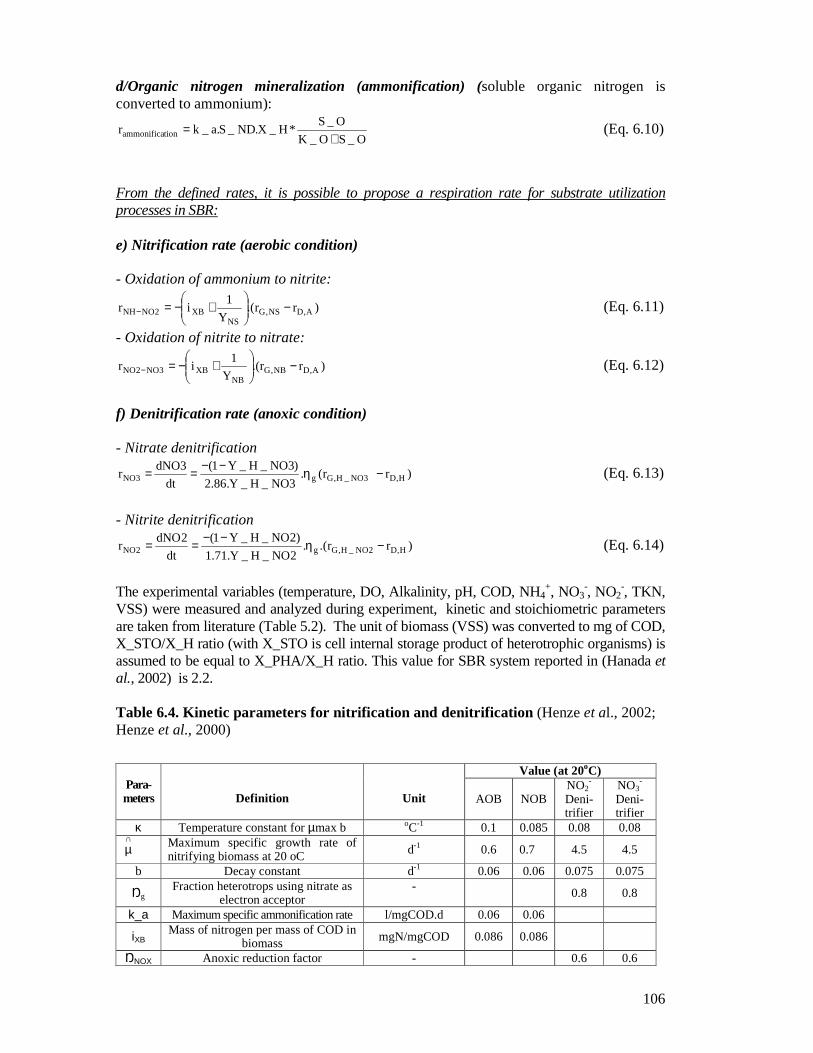
106

d/Organic nitrogen mineralization (ammonification) (soluble organic nitrogen is converted to ammonium):

O_SO_K

O_S*H_X.ND_S.a_kr tionammonifica +

= (Eq. 6.10)

From the defined rates, it is possible to propose a respiration rate for substrate utilization processes in SBR: e) Nitrification rate (aerobic condition) - Oxidation of ammonium to nitrite:

)rr.(Y

1ir A,DNS,G

NSXB2NONH −

+−=− (Eq. 6.11)

- Oxidation of nitrite to nitrate:

)rr.(Y

1ir A,DNB,G

NBXB3NO2NO −

+−=− (Eq. 6.12)

f) Denitrification rate (anoxic condition) - Nitrate denitrification

)rr(.3NO_H_Y.86.2

)3NO_H_Y1(

dt

3dNOr H,D3NO_H,Gg3NO −η−−== (Eq. 6.13)

- Nitrite denitrification

)rr.(.2NO_H_Y.71.1

)2NO_H_Y1(

dt

2dNOr H,D2NO_H,Gg2NO −η−−== (Eq. 6.14)

The experimental variables (temperature, DO, Alkalinity, pH, COD, NH4

+, NO3-, NO2

-, TKN, VSS) were measured and analyzed during experiment, kinetic and stoichiometric parameters are taken from literature (Table 5.2). The unit of biomass (VSS) was converted to mg of COD, X_STO/X_H ratio (with X_STO is cell internal storage product of heterotrophic organisms) is assumed to be equal to X_PHA/X_H ratio. This value for SBR system reported in (Hanada et al., 2002) is 2.2.

Table 6.4. Kinetic parameters for nitrification and denitrification (Henze et al., 2002; Henze et al., 2000)

Value (at 20oC)

Para-meters

Definition

Unit AOB NOB

NO2-

Deni- trifier

NO3-

Deni-trifier

κ Temperature constant for µmax b oC-1 0.1 0.085 0.08 0.08 ∩µ

Maximum specific growth rate of nitrifying biomass at 20 oC d-1 0.6 0.7 4.5 4.5

b Decay constant d-1 0.06 0.06 0.075 0.075

Ŋg Fraction heterotrops using nitrate as

electron acceptor - 0.8 0.8

k_a Maximum specific ammonification rate l/mgCOD.d 0.06 0.06

iXB Mass of nitrogen per mass of COD in

biomass mgN/mgCOD 0.086 0.086

ŊNOX Anoxic reduction factor - 0.6 0.6

107

YA Maximum yield coefficient mgCOD/mgNO3-

produced 0.11 0.06

YH Maximum yield coefficient mgCOD/mgNO3- 1.7 1.7

KN Saturation constant for ammonium or

nitrite mgN/L 0.5 1

KNO Saturation constant for nitrite or nitrate mgN/L 0.35 0.35 KDO Saturation constant for oxygen mgO2/L 0.75 1 0.3 0.3 KAKL Saturation constant for alkalinity mgHCO3

-/L 30.5 30.5 KCOD Saturation constant for COD mgO2/L 15 15

KSTO Saturation constant for XSTO mgCOD(XSTO)/mgCOD(XH) 1 1

Specific growth rates of ammonium and nitrite nitrifying bacteria at given temperature (21.2 oC) are 0.42 and 0.39 (d-1) respectively. Average nitrification rates (mgN/L.h) in the total experimental time are compared to nitrification rates calculated with Monod equations Eq.6.1-6.4; Eq.6.8, Eq.6.11 and Eq.6.12 (using parameters mentioned in Table 5.2). By fitting value of concentration of Ammonium oxidizing bacteria (AOB) and Nitrite oxidizing bacteria (NOB) to fit the two values of nitrification rate (using parameters mentioned in Table 5.2) (for more detail see Annex 6.2), we can estimate the proportion of (AOB) and (NOB). Estimated proportion of active AOB and NOB in the experimental day 29 February 2007 is about 1.13 % and 0.63 % of VSS (22 and 12.4 mg/L), respectively, corresponding to biomass activity around 1.54 mgN/gVSS.h. The concentration of NOB is smaller compared to AOB due to limitation of oxygen during partial nitrification. Minimum SRT (calculated by θmin = 1/(µ-b)) should be kept around 2.8 (d) for AOB and 3.0 d for NOB so that the system does not lose biomass. For the denitrification process, specific growth rates at given temperature of nitrite and nitrate denitrifying bacteria are 1.56 and 0.82 (d-1) respectively. Average denitrification rates (mgN/L.h) during denitrification time are also fit together by using Eq. 6.5-6.7, Eq. 6.9, Eq. 613-6.14 to calculate denitrifying bacterias (using parameters mentioned in Table 5.2) (for more detail see Annex 6.2) . Proportion of active Nitrite denitrifying bacteria and Nitrate denitrifying bacteria is evaluated around 23.8% and 2.17 % of VSS (461 and 42.3 mg/L), respectively. However, the concentration of the later could be higher if more nitrates were produced during the nitrification process. Minimum SRT should be kept at least 1.77 d for denitritant and 2.30 (d) for denitratant. However, when the ANAMMOX process is considered, this SRT will have to be increased.

6.3.6. Optimization of the partial nitrification Observations of the influence of working conditions on nitrite accumulation (necessary for partial nitrification) as well as nitrification and denitrification efficiency were done with concentration of dissolved oxygen (DO) and free ammoniac (free NH3) in the first step of the study, which is presented in this part. The influence of DO on nitrite accumulation in nitrification process is significant. The nitrite accumulation increases when DO decreases, this shows capability to get partial nitrification in SBR. Graph 5.2, 5.3 and 5.4 present nitrogen removal evolution when average DO during the period of nitrification is controlled around 7.5, 3.8 and 1.5 mg/L.

108

N removal evolutionCycle: 4h Nitrification - 4h Denitrification

DO ~ 1.5 mg/L

0

20

40

60

80

100

0 1 2 3 4 5 6 7 8

Time (h)

NH

4+N

(m

g/L

)

0

5

10

15

NH4+N

NO2-N

NO3-N

Nitrification Denitrificatio

NO

2-N

or

NO

3-N

(m

g/L)

N removal evolutionCycle: 4h Nitrification - 4h Denitrification

DO ~ 7.5 mg/L

0.0

20.0

40.0

60.0

80.0

100.0

0 1 2 3 4 5 6 7 8

Time (h)

NH

4+N

(m

g/L)

0.0

5.0

10.0

15.0

20.0

25.0

NH4+N

NO2-N

NO3-N

Nitrification Denitrification

NO

2-N

or

NO

3-N

(m

g/L)

N removal evolutionCycle: 4h Nitrification - 4h Denitrification

DO ~ 3.8 mg/L

0

20

40

60

80

100

0 1 2 3 4 5 6 7 8

Time (h)

NH

4+N

(m

g/L)

0

5

10

15

20

25

NH4+N

NO2-N

NO3-N

Nitrification Denitrification

NO

2-N

or

NO

3-N

(m

g/L)

Graph 6.3. Nitrogen removal evolution 1, pH = 7.79, To = 19oC, VSS = 1.93 g/L

Graph 6.4. Nitrogen removal evolution 2, pH = 8.04, To = 19.7oC

NO2/(NO2+NO3) versus DO[NH4] ~ 80 mgN/L

0.70

0.75

0.80

0.85

0.90

0.00 0.50 1.00 1.50 2.00 2.50

DO (mg/L)

NO

2/(N

O2+

NO

3)

NO2/(NO2+NO3)

Graph 6.5. Nitrogen removal evolution 3, pH = 7.84, To = 19.2, VSS =1.81 g/L

Graph 6.6. Influence of DO on nitrite accumulation

Concentration of DO that is suitable for the partial nitrification process is around 0.8-2.2 mg/L. Among the three values of DO used to control the process (1 mg/L, 1.5 mg/L and 2 mg/L) it is found that with DO ~ 1mg/L the system yields the best nitrite accumulation and not with DO ~ 2mg/L (Graph 5.5). But the result is opposite when N removal efficiency is concerned. With DO of 1.5 mg/L, the system obtains an intermediate result. It is obvious that, with a DO of 1.5 mg/L, nitrate is almost not produced; there is a nitrite accumulation of 88 %. However, ammonium removal efficiency in this case is still limited (17 %), and as a result the nitrite produced is fully consumed before the end of denitrification period. Working time therefore was modified to improve the nitrification efficiency, to get a 50/50 ratio of ammonium (remaining)/nitrite (produced), meanwhile avoiding to waste time and energy in the denitrification process. Time of aeration phase (nitrification) was changed from 4 hours to 5 hours and then 6 hours. As a result, time of mixing phase (denitrification) was changed from 4 hours to 3 hours and then 2 hours, respectively. Graph 5.6 and 5.7 present nitrogen removal evolution of those time cycles. DO concentration is still controlled around 1.5 mg/L. It is found that, the cycle of 6 hours-nitrification and 2 hours – denitrification (Graph 5.7) got a better nitrite accumulation, which is up to 89 % and an improved ammonium removal efficiency of 24 %. The nitrification process, however has not yet reached a 50/50 ammonium/nitrite ratio. Other factors such as temperature, HRT, SRT and also DO will be modified in the next step in SHARON process. Total ammonium oxidized is always higher than total nitrite and nitrate produced in nitrification (about 57%), suggesting that

109

N removal evolutionCycle: 5h Nitrification - 3h Denitrification

DO ~ 1.5 mg/L

0

20

40

60

80

100

0 1 2 3 4 5 6 7 8

Time (h)

NH

4+N

(m

g/L)

0

3

6

9

12

NH4+N

NO2-N

NO3-N

Nitrification Denitrification

NO

2-N

or

NO

3-N

(m

g/L)

N removal evolutionCycle: 6h Nitrification - 2h Denitrification

DO ~ 1.5 mg/L

0

20

40

60

80

100

0 1 2 3 4 5 6 7 8

Time (h)

NH

4+N

(m

g/L)

0

3

6

9

12

15

NH4+N

NO2-N

NO3-N

Nitrification Denitrification

NO

2-N

or

NO

3-N

(mg/

L)

NO2-N/(NO2-N+NO3-N) and NH4+ removal efficiency versus free NH3

0

20

40

60

80

100

0.0

0.5

1.0

1.5

2.0

2.5

3.0

3.5

4.0

4.5

Free NH3 (mgN/L)

NO

2 ac

cum

ulat

ion/

NH

4 re

mov

al e

ffici

ency

NO2-N/(NO2-N+NO3-N)(%)

NH4+ removaleff iciency(%)

Simultaneous Nitrification Denitrification (SND) phenonmena could take place. It is expected to get a higher value of nitrogen removal efficiency and an expected ratio of ammonium/nitrite when these working conditions (especially temperature and also dissolved oxygen) are controlled more strictly in the SHARON process.

Graph 6.7. Nitrogen removal evolution 4, pH = 8.11, To = 19.9 , VSS = 1.95 g/L

Graph 6.8. Nitrogen removal evolution 5, pH = 7.92, To = 19.1, VSS = 1.92 g/L

Free NH3 was calculated according to the Eq. 5.14 (Verstraete and van Vaerenberg, 1985), (Eq. 6.14) Influence of free NH3 on NO2-N/(NO2-N+NO3-N) and NH4

+ removal efficiency is also obvious. With a free NH3 concentration of 1.6 mgN/L, the system already obtains an accumulation of 75% of NO2

- (Graph 5.8). But NH4+ removal efficiency is lower when free

NH3 increases. According to the results presented by (Anthonisen et al., 1976), a partial inhibition of the ammonium nitrifiers is observed from 10 mgN-NH3/L and the inhibition is complete at 150 mgN/L. For nitrite nitrifiers, the partial and total inhibition levels were estimated at 0.1 and 1 mgN/L, respectively. In contrast, the results obtained by (Belline et al., 2007) indicated no inhibition of ammonium nitrifiers or nitrite nitrifiers by free NH3 up to 50 mgN/L. As mentioned by Villaverde et al. (2000), acclimatisation of the bacteria could explain the different inhibition levels reported in the literature (Tabares, 2006).

Graph 6.9. Influence of free NH3 on nitrite ccumulation

)T0241.0ln(10*398.310

10

)NHNH(

NH9pH

pH

43

3

−=

+∑ +

110

6. 4. CONCLUSION OF THE CHAPTER The system is well-mixed for both nitrification and denitrification processes. It is necessary to increase the aeration rate (e.g. Kla value) to supply enough oxygen for the nitrification process and possibly to avoid Simultaneous Nitrification Denitrification (SND) phenomena in partial nitrification. Although time for settling phase is just enough but the latest value of SVI measured is still high (250 mL/g). This value needs to be improved by eliminating suspended solid in inlet leachate or even increasing the minimum working volume of SBR. Mathematical model based on modified ASM1 and ASM3 helped to determine some kinetic parameters of the process (e.g. special growth rate at given temperature µ(T)) of AOB, NOB, Nitrite denitrifers and Nitrate denitrifiers. The concentrations of those main micro-organisms were also estimated by fitting value of nitrification rate (mgN/L.h) obtained directly from experiment and calculation with Monod equations of the model. These values have to be confirmed by other testing methods (e.g. FISH) to estimate the accuracy of other kinetic or stoichiometric parameters. The nitrite accumulation increases when DO decreases, confirming the SBR capability for partial nitrification. Concentration of DO that is suitable for this process is around 0.8-2.2 mg/L with the best value of 1.5 mg/L. The working cycle of 6 hours Nitrification/2 hours Denitrification has shown the best nitrite accumulation of the SBR but not yet yielding a 50/50 ratio of ammonium/nitrite at the end of nitrification process. A well managed SHARON process will be processed in the next step of the study to obtain higher nitrogen removal efficiency and the expected ratio of ammonium/nitrite. Influence of free NH3 on NO2-N/(NO2-N+NO3-N) was also obvious. With concentration of free NH3 around 1.6 mgN/L, the system already obtained an accumulation of 75% NO2

--N.

111

REFERENCES

1. Anthonisen, A. C., R. C. Loehr, T. B. Prakasam, and E. G. Srinath, 1976, Inhibition of nitrification by ammonia and nitrous acid: J. Water Pollut. Control Fed., v. 48, p. 835-852.

2. ASCE, 1992, Measurement of Oxygen Transfer in Clean water. , American Society of Civil Engineers, New York.

3. Belline, F., H. Boursier, F. Guiziou, and E. Paul, 2007, Modelling of biological nitrogen removal during treatment of piggery wastewater: Water Science & Technology Q IWA Publishing, v. 55 p. 11–19

4. Benefield, L. D., and C. W. Randall, 1980, Biological Process Designed for Wastewater Treatment, Prentice-Hall, Inc., Englewood Cliffs, N.I.

5. Hanada, S., H. Satoh, and T. Mino, 2002, Measurement of microorganisms with PHA production capability in activated sludge and its implication in Activated Sludge Model No. 3: Water Science and Technology v. 45, p. 107–113.

6. Henze, M., P. Harremoes, J. L. C. Jansen, and E. Arvin, 2002, Wastewater Treatment: Biological and Chemical Processes: ISBN 3-540-42228-5, Springer - Verlag Berlin Heidelberg, Germany.

7. Henze, M., W. Gujer, T. Mino, and M. van Loosdrecht, 2000, Activated Sludge Models ASM1, ASM2, ASM2d and ASM3 in I. T. G. o. M. M. F. D. a. O. o. B. W. Treatment, ed., Scientific and Technical Report No. 9, IWA publishing, London, UK.

8. Metcalf&Eddy, 1991, Wastewater Engineering. Treatment, Disposal and Reuse: New York, Mc Graw - Hill Book Company. , 1771 p.

9. Savitsky, A., and M. J. E. Golay, 1964, Smoothing and di®erentiation of data by simplied least squares proceduresx: Analytica Chimica Acta, v. 36, p. 1627-1639.

10. Spanjers, H., and P. Vanrolleghem, 1995, Respirometry as a tool for rapid characterization of wastewater and activated sludge: Water Science and Technology, v. 31, p. 105-114.

11. Tabares, L. C., 2006, Control and optimization of an SBR for nitrogen removal: From model calibration to plant operation, Universitat de Girona, Girona, 231 p.

12. Verstraete, W., and E. van Vaerenberg, 1985, Aerobic activated sludge Biotechnology. 8, H.J. Rehm editor VCH, p. 41 - 44.

112

113

CHAPTER VII

TESTS FOR DETERMINATION OF MAXIMUM NITRIFICATION AND DENITRIFICATION CAPABILITY AND KINETIC AND STOICHIOMETRIC PARAMETERS

7.1. TEST FOR DETERMINATION OF MAXIMUM NITRIFICATIO N AND DENITRIFICATION CAPABILITY

7.1.1. Materials This part of the research has been done in Vietnam, in the Vietnamiese Academy of Science and Technology, Single reactor: 4.5L (45 cm x 20 cm x 10 cm), working volume 2L, installed with aerator (nitrification reactor _ B1) and mixer (denitrification reactor _B2) (Figure 7.1).

Figure 7.1. Test reactors to determine the maximum nitrification and denitrification capability (B1 and B2) and kinetic and stoichiometric parameters of activated sludge (B3)

Summary: The first part of this chapter presents the experimental studies on maximum nitrification and denitrification capability. The main achivements of this part are given in “Results and discussion”. The second part of the study is determination of kinetic and stoichiometric parameters that will be used for calibration in the next steps (Chapter IX). The main kinetic and stoichiometric parameters are found from these tests include maximum growth rate, decay rate and yield coefficient of ammonium oxidizing bacteria, nitrite oxidizing bacteria and yield coefficient of heterotrophic bacteria.

114

Activated sludge Sludge was collected at Domestic WWTP Kim Lien – Truc Bach, Hanoi. This sludge, was kept in a container, continuously aerated and fed with leachate, NH4Cl and alkalinity NaHCO3 during one month, and has shown a good activity for ammonium removal. A part of this sludge was used for the experiments. Leachate: Leachates were collected at the biological pond in Nam Son landfill site. They were characterized by an ammonium concentration of 24.5 mgN/L, COD of 303 mgO2/L (considered as inert COD), CaCO3 of 210 mg/L and pH of 8.13. This leachate was used as a background environment for the experiments. Chemicals: NH4Cl, NaHCO3 were injected at the beginning of nitrification process. When working at the influence of COD on nitrification process, yellow sugar (as carbon source) was added. NaNO2, KNO3 and sugar (as COD) were injected at the beginning of denitrification process. Together with sugar, only NaNO2 or KNO3 was added when NUR1 or NUR2 was observed alone. Two chemicals, NaNO2 and KNO3, were added when total NUR was observed.

7.1.2. Working condition For both B1 and B2, the working time was 6 hours. Temperature during experiments time was around 26.7 – 28.5 oC. Sludge age was kept stable during experimental times at 10 days. Sludge concentration was kept in B1 around 2.5 g MLSS/L (~ 2 gMLVSS/L) and in B2 around 4.5 g MLSS/L (4 g MLVSS/L) respectively. In B1, at the first step, ammonium uptake rate (AUR), nitrite production rate (NPR1) and nitrate production rate (NPR2) together with biomass activity and NO2

-/(NO2-+NO3

-) were observed when ammonium concentration was modified six times: 100 mgN/L, 150 mgN/L, 200 mgN/L, 250 mgN/L, 300 mgN/L and 400 mgN/L. Then, with the above ammonium concentrations (except of the concentration of 100 and 150 mgN/L), carbon source was added at the beginning of the process with a same amount so that biodegradable COD was around 300 mgO2/L. AUR, NPR1 and NPR2 were observed with influence of COD. In B2, nitrite uptake rate (NUR1), nitrate uptake rate (NUR2) and total of nitrate and nitrite uptake rate (NPR) together with biomass activity were observed. Firstly, NUR1 was observed alone, and then secondly was NUR2. Finally, both NUR1 and NUR2 were observed together with NUR. All experiments with different conditions were conducted at least three times; the values of experiments are average values of repeated tests.

115

Nitrification: NH4 ~ 100mgN/Ly = -17.929x + 136.71

R2 = 0.9903

y = 15.241x - 8.5357R2 = 0.991

y = 2.3804x - 2.3286R2 = 0.9313

0

20

40

60

80

100

120

140

0 2 4 6 8Time (hour)

N (

mgN

/L)

0

200

400

600

800

1000

1200

NH4NO2NO3Alkalinity

Alk

alin

ity (

mgC

aCO

3/L)

Nitrification: NH4 ~ 150mgN/L

y = -25.688x + 179.57R2 = 0.9929

y = 23.139x - 18.443R2 = 0.9718

y = 3.0446x - 1.1786R2 = 0.9075

0

50

100

150

200

0 2 4 6 8Time (hour)

N (

mgN

/L)

0

500

1000

1500

2000

NH4NO2NO3AlkalinityLinear (NH4)

Alk

alin

ity (

mgC

aCO

3/L)

Nitrification: NH4 ~ 200mgN/L

y = -31.214x + 245.57R2 = 0.9855

y = 29.232x - 37.357R2 = 0.9792

y = 3.325x - 3.2429R2 = 0.9265

0

50

100

150

200

250

0 2 4 6 8Time (hour)

N (m

gN/L

)

0

500

1000

1500

2000

2500

NH4NO2NO3AlkalinityLinear (NH4)

Alk

alin

ity (

mgC

aCO

3/L)

Nitrification: NH4 ~ 250mgN/Ly = -33.393x + 301

R2 = 0.9841

y = 30.102x - 26.3R2 = 0.9806

y = 3.6536x - 6.1429R2 = 0.9417

0

50

100

150

200

250

300

0 2 4 6 8Time (hour)

N (

mgN

/L)

0

500

1000

1500

2000

2500

NH4NO2NO3AlkalinityLinear (NH4)

Alk

alin

ity (

mgC

aCO

3/L)

7.1.3. Results and discussions

7.1.3.1. Test to determine the maximum nitrification capability in B1 a) AUR, NPR1 and NPR2, biomass activity and NO2

-/(NO2-+NO3

-) without the influence of COD. Graphs 7.1 to 7.6 show nitrification profile of experiments with ammonium concentration of 100 to 400 mgN/L. Temperature during experiments changed from 26.7 to 28.5oC. SS was kept in the same value during the batch experiments, of around 2.5 g/L, corresponding to VSS of 2 g/L. pH at the beginning of each test is around 8.12 - 8.33. Alkalinity is added together with ammonium with a ratio of CaCO3/NH4

+ ~ 7.14. DO was not recorded during the tests, but intensity of DO supply was kept the same during all the tests with a Kla of 18.35 h-1 (this Kla will be used as the highest value in the next experiment). The evolution of alkalinity also fits well with the evolution of ammonium.

Graph 7.1. Nitrification process with [NH4+] ~ 100 mgN/L

Graph 7.2. Nitrification process with [NH4+] ~ 150 mgN/L

Graph 7.3. Nitrification process with [NH4+] ~ 200 mgN/L

Graph 7.4. Nitrification process with [NH4+] ~ 250 mgN/L

116

Nitrification: NH4 ~ 300mgN/Ly = -36.964x + 340.86

R2 = 0.9948

y = 34.67x - 27.714R2 = 0.9837

y = 3.7125x - 0.5429R2 = 0.9637

050

100150200250300350

0 1 2 3 4 5 6 7 8

Time (hour)

N (

mgN

/L)

0

500

1000

1500

2000

2500

3000

NH4NO2NO3AlkalinityLinear (NH4)

Alk

alin

ity (

mgC

aCO

3/L)

NH4 versus AUR, NPR1, NPR2 y = -0.0003x2 + 0.1996x + 1.4019

R2 = 0.9885

y = -0.0003x2 + 0.202x - 1.628

R2 = 0.9809

y = -5E-05x2 + 0.028x + 0.0775

R2 = 0.9652

011223344

0 50 100 150 200 250 300 350 400 450 500

NH4 (mgN/L)

AU

R, N

PR

1, N

PR

2 (m

gN/L

.h)

0

10

20

30

40

50

NPR2AURNPR1Poly. (AUR)Poly. (NPR1)Poly. (NPR2)

NH4 versus Biomass activity and NO2/(NO2+NO3)

y = -0.0001x2 + 0.1028x + 0.1914

R2 = 0.9912

y = 0.0002x + 0.8479

R2 = 0.9129

0.0

5.0

10.0

15.0

20.0

25.0

0 100 200 300 400 500

NH4 (mgN/L)

Bio

mas

s ac

tivity

(m

gN/g

VS

S.h

)

0.86

0.88

0.90

0.92

0.94

Biomass activity

NO2/(NO2+NO3)

Poly. (Biomassactivity)

Linear(NO2/(NO2+NO3))

NO

2/(N

O2+

NO

3)

Nitrification: NH4 ~ 400mgN/Ly = -37.679x + 406.57

R2 = 0.9607

y = 35.731x - 35.057R2 = 0.9971

y = 2.4714x - 0.5429R2 = 0.8957

0

100

200

300

400

500

0 1 2 3 4 5 6 7 8

Time (hour)

N (

mgN

/L)

05001000150020002500300035004000

NH4NO2NO3AlkalinityLinear (NH4)

Alk

alin

ity (

mgC

aCO

3/L)

Graph 7.5. Nitrification process with [NH4+] ~ 300 mgN/L

Graph 7.6. Nitrification process with [NH4+] ~ 400 mgN/L

The Table 7.1 gives the results of AUR, NPR1, NPR2, biomass activity and also NO2

-

/(NO2-+NO3

-) of experiments with 6 different concentrations of ammonium at the beginning of the tests. Table 7.1. The results of AUR, NPR1, NPR2, biomass activity and NO2-/(NO2-+NO3-)

[NH4] (mgN/L) 100 150 200 250 300 400 Biomass activity mgN/gVSS.h 8.8 12.84 15.61 16.70 18.48 19.20 NO2/(NO2+NO3) 0.865 0.884 0.898 0.892 0.903 0.94 AUR mgN/L.h 17.9 26.3 31.2 33.4 37.0 38.39 NPR1 mgN/L.h 15.2 23.1 29.2 30.1 34.7 35.73 NPR2 mgN/L.h 2.38 3.04 3.33 3.65 3.71 2.47

And Graphs 7.7 and 7.8 present values in the Table 7.1 in curves.

Graph 7.7. AUR, NPR1, NPR2 evolution with different [NH4+]

Graph 7.8. Biomass activity and NO2/(NO2+NO3) with different [NH4+]

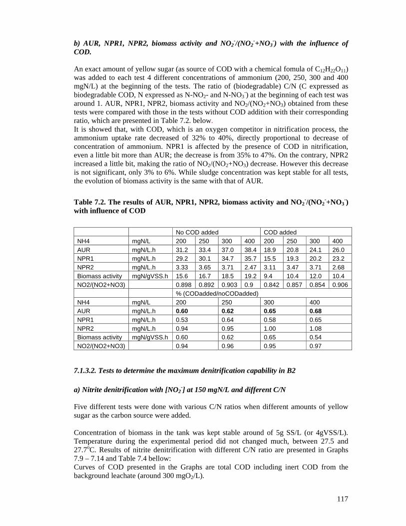
117

b) AUR, NPR1, NPR2, biomass activity and NO2-/(NO2

-+NO3-) with the influence of

COD. An exact amount of yellow sugar (as source of COD with a chemical fomula of C12H22O11) was added to each test 4 different concentrations of ammonium (200, 250, 300 and 400 mgN/L) at the beginning of the tests. The ratio of (biodegradable) C/N (C expressed as biodegradable COD, N expressed as N-NO2- and N-NO3

-) at the beginning of each test was around 1. AUR, NPR1, NPR2, biomass activity and NO2/(NO2+NO3) obtained from these tests were compared with those in the tests without COD addition with their corresponding ratio, which are presented in Table 7.2. below. It is showed that, with COD, which is an oxygen competitor in nitrification process, the ammonium uptake rate decreased of 32% to 40%, directly proportional to decrease of concentration of ammonium. NPR1 is affected by the presence of COD in nitrification, even a little bit more than AUR; the decrease is from 35% to 47%. On the contrary, NPR2 increased a little bit, making the ratio of NO2/(NO2+NO3) decrease. However this decrease is not significant, only 3% to 6%. While sludge concentration was kept stable for all tests, the evolution of biomass activity is the same with that of AUR.

Table 7.2. The results of AUR, NPR1, NPR2, biomass activity and NO2-/(NO2

-+NO3-)

with influence of COD

No COD added COD added NH4 mgN/L 200 250 300 400 200 250 300 400 AUR mgN/L.h 31.2 33.4 37.0 38.4 18.9 20.8 24.1 26.0 NPR1 mgN/L.h 29.2 30.1 34.7 35.7 15.5 19.3 20.2 23.2 NPR2 mgN/L.h 3.33 3.65 3.71 2.47 3.11 3.47 3.71 2.68 Biomass activity mgN/gVSS.h 15.6 16.7 18.5 19.2 9.4 10.4 12.0 10.4 NO2/(NO2+NO3) 0.898 0.892 0.903 0.9 0.842 0.857 0.854 0.906 % (CODadded/noCODadded) NH4 mgN/L 200 250 300 400 AUR mgN/L.h 0.60 0.62 0.65 0.68 NPR1 mgN/L.h 0.53 0.64 0.58 0.65 NPR2 mgN/L.h 0.94 0.95 1.00 1.08 Biomass activity mgN/gVSS.h 0.60 0.62 0.65 0.54 NO2/(NO2+NO3) 0.94 0.96 0.95 0.97

7.1.3.2. Tests to determine the maximum denitrification capability in B2 a) Nitrite denitrification with [NO2

-] at 150 mgN/L and different C/N Five different tests were done with various C/N ratios when different amounts of yellow sugar as the carbon source were added. Concentration of biomass in the tank was kept stable around of 5g SS/L (or 4gVSS/L). Temperature during the experimental period did not changed much, between 27.5 and 27.7oC. Results of nitrite denitrification with different C/N ratio are presented in Graphs 7.9 – 7.14 and Table 7.4 bellow: Curves of COD presented in the Graphs are total COD including inert COD from the background leachate (around 300 mgO2/L).

118

Nitrite Denitrification with [NO2-] ~ 150mgN/L C/N ~ 1.88

0

50

100

150

200

0h 1h 2h 3h 4h 5h

Time (hour)

N (

mgN

/L)

0

500

1000

1500

2000

CO

D,

Alk

alin

ity

(mg/

L)

COD

Alkalinity

NO2

Nitrite Denitrification with [NO2-] ~ 150mgN/LC/N ~ 6.49

0

50

100

150

200

0h 1h 2h

Time (hour)

NO

2- (

mgN

/L)

0

500

1000

1500

CO

D,

Alk

alin

ity

(mg/

L)

NO2

COD

Alkalinity

Nitrite Denitrification with [NO2-] ~ 150mgN/LC/N ~ 4.97

020406080

100120140160

0h 1h 2h

Time (hour)

N (

mgN

/L)

0

400

800

1200

1600

CO

D,

Alk

alin

ity

(mg/

L)

NO2

COD

Alkalinity

Nitrite Denitrification with [NO2-] ~ 150mgN/LC/N ~ 3.92

0

50

100

150

200

0h 1h 2h

Time (hour)

N (

mgN

/L)

0

500

1000

1500

CO

D,

Alk

alin

ity

(mg/

L)

NO2

COD

Alkalinity

Nitrite Denitrification with [NO2-] ~ 150mgN/LC/N ~ 3.17

0

50

100

150

200

0h 1h 2h 3h 4h 5h

Time (hour)

N (

mgN

/L)

0

500

1000

1500

2000

CO

D,

Alk

alin

ity

(mg/

L)

COD

Alkalinity

NO2

Nitrite denitrification with different C/N

0

50

100

150

200

0 2 4 6 8

COD/NO2

NU

R1

(mg

N/L

.h)

NUR1

Biomass activity

Graph 7.9. Nitrite denitrification with C/N ~ 6.49

Graph 7.10. Nitrite denitrification with C/N ~ 4.97

Graph 7.11. Nitrite denitrification with C/N ~ 3.92

Graph 7.12. Nitrite denitrification with C/N ~ 3.17

Graph 7.13. Nitrite denitrification with C/N ~ 1.88

Graph 7.14. Effect of the C/N ration on Nitrite denitrification ( pH= 8.38, t° = 27.6oC; VSS = 4g/L)

119

Nitrate denitrification with [NO3] ~ 150mgN/L C/N ~ 11.86

020406080

100120140160180

0h 1h 2h 3h 4h

Time (hour)

N (

mgN

/L)

0

500

1000

1500

2000

2500

NO3

COD

Alkalinity

NO2

CO

D,

Alk

alin

ity

(mg/

L)

Nitrate denitrification with [NO3] ~ 150mgN/LC/N ~ 9.64

020406080

100120140160

0h 1h 2h 3h 4h

Time (hour)

N (

mgN

/L)

0

500

1000

1500

2000

2500

NO3

COD

Alkalinity

NO2

CO

D,

Alk

alin

ity

(mg/

L)

Table 7.3. NUR1 and biomass activity with different C/N (pH= 8.38, t° = 27.6oC; VSS = 4g/L

COD/NO2 mgCOD/mgN 6.49 4.97 3.92 3.17 1.88 NUR1 mgN/L.h 149.3 135.7 76.5 36.0 24.6 Biomass activity mg/gVSS.h 41.5 37.7 20.3 10.5 6.8

Obviously the C/N ratio has an important effect on the kinetic of denitrification. Above 5, a theoretical threshold value is reached, as the heterotroph are not limited by the carbon source anymore. Below the kinetic of denitrification depends on the C/N ratio. b) Nitrate denitrification with [NO3

-] at 150 mgN/L and different C/N Also five tests were done with various C/N ratios when different amounts of yellow sugar as the carbon source were added. Concentration of biomass in the tank was kept stable around 5g SS/L (or 4gVSS/L). Temperature during the experimental period was between 27 and 27.5oC. Results of nitrite denitrification with different C/N ratio are presented in Graph 7.15 – 7.20 and Table 7.6 bellows: Curves of COD presented in the Figures are included also inert COD from the background leachate (around 300 mgO2/L).

Graph 7.15 Nitrate denitrification with C/N ~ 11.86

Graph 7.16 Nitrate denitrification with C/N ~ 9.64

120

Nitrate denitrification with [NO3] ~ 150mgN/L C/N ~ 5.27

020406080

100120140160

0h 1h 2h 3h 4h 5h 6h

Time (hour)

N (

mgN

/L)

0

200400

600

800

10001200

1400

NO3

COD

Alkalinity

NO2

CO

D,

Alk

alin

ity

(mg/

L)

NO3 denitrification with different C/N

0

10

20

30

40

50

60

0 2 4 6 8 10 12 14

COD/NO3

NU

R2

(mgN

/L.h

)

NUR2

Biomass activity

Nitrate denitrification with [NO3] ~ 150mgN/LC/N ~ 6.34

020406080

100120140160180

0h 1h 2h 3h 4h

Time (hour)

N (

mgN

/L)

0

500

1000

1500

2000

NO3

COD

Alkalinity

NO2

CO

D,

Alk

alin

ity

(mg/

L)

Nitrate denitrification with [NO3] ~ 150mgN/LC/N ~ 3.22

020406080

100120140160

0h 1h 2h 3h 4h 5h 6h

Time (hour)

N (

mgN

/L)

0

200

400

600

800

1000

1200

NO3

COD

Alkalinity

NO2

CO

D,

Alk

alin

ity

(mg/

L)

Graph 7.17 Nitrate denitrification with C/N ~ 6.34

Graph 7.18 Nitrate denitrification with C/N ~ 5.27

Graph 7.19 Nitrate denitrification with C/N ~ 3.22

Graph 7.20 Effect of the C/N ration on Nitrate denitrification ( pH= , t° =; SS = )

Table 7.4. NUR2 and biomass activity with different C/N

COD/NO3 mgCOD/mgN 11.86 9.64 6.34 5.27 3.22 NUR2 mgN/L.h 51.5 48.9 38.1 23.92 15.5 Biomass activity mg/gVSS.h 14.1 13.4 10.5 6.43 3.6

c) Nitrite and nitrate denitrification with different [NO3

-] and [NO2-] and the same C/N

Three different tests were done with the same C/N ratio when different amounts of yellow sugar as the carbon source were added into the tank with different concentrations of nitrite and nitrate. Concentration of biomass in the tank was kept stable around 5g SS/L (or 4gVSS/L). Temperature during the experimental period was between 27 and 28.5oC. Results of nitrite denitrification with different concentration of nitrite and nitrate are presented in Graphs 7.21 – 7.23 and Table 7.8 bellow: Curves of COD presented in the Figures include also inert COD from the background leachate (around 300 mgO2/L).

121

Denitrification: [NO2]~150mgN/L, [NO3]~150mgN/L, COD/N = 6.47

0

50

100

150

200

250

300

0h 1h 2h 3h 4h 5h 6h

Time (hour)

N (

mgN

/L)

0

500

1000

1500

2000

2500

CO

D,

CaC

O3

(mg/

L)

Alkalinity

NO3

NO2

NO2+NO3

COD

Denitrification: [NO2]~50mgN/L, [NO3]~50mgN/L, COD/N = 6.23

0

50

100

150

0h 1h 2h 3h 4h 5h 6h

Time (hour)

N (

mgN

/L)

0

500

1000

1500

CO

D,

CaC

O3

(mg/

L)

NO3

COD

Alkalinity

NO2

NO2+NO3

Denitrification: [NO2]~100mgN/L, [NO3]~100mgN/L, COD/N = 6.46

0

50

100

150

200

250

0h 1h 2h 3h 4h 5h 6h

Time (hour)

N (

mgN

/L)

0

500

1000

1500

2000

CO

D,

CaC

O3

(mg/

L)

NO3

NO2

NO2+NO3

COD

Alkalinity

Graph 7.21 Nitrite and nitrate denitrification with C/N ~ 6.23

Graph 7.22 Nitrite and nitrate denitrification with C/N ~ 6.46

Graph 7.23 Nitrite and nitrate denitrification with C/N ~ 6.47

Table 7.5. NUR1 and NUR2 and biomass activity with different C/N

NO2, NO3 mgN/L 50 100 150 C/N mgCOD/mgN 6.23 6.46 6.47 NUR1 mgN/L.h 20.3 24.8 27.7 NUR2 mgN/L.h 28.2 33.8 34.1 NUR1+NUR2 mgN/L.h 48.5 58.6 61.8 Biomass activity mg/gVSS.h 11.5 13.3 14.4

7.2. BIOACTIVITY ESSAYS TO DETERMINE KINETIC AND STOICHIOMETRIC PARAMETERS OF ACTIVATED SLUDGE This test was done based on variable values of hydraulic retention time (HRT) and solid resident time (SRT) (Metcalf&Eddy, 1991). Kinetic and stoichiometric parameters determined were: µH, µA, YH, YA, bH, bA, KS, KN. Concentration of substrate is kept constant. SRT is calculated by total sludge in the reactor divided by the flux wasted out the system.

122

Hypothesis: rus = dS/dt = -(So-S)/θ = -k.XS/(Ks+S) where rus is rate of substrate utilization, θ is HRT (d), S is substrate (mg/L), k is substrate consumption coefficient, Ks is haft-coefficient of substrate (mg/L), X is concentration of biomass (mg/L). θX/(So-S) = 1/k + Ks/kS y = 1/k + x.Ks/k � 1/k � Ks 1/θc=-Y.rsu/X – kd where θc is SRT (d), Y is yield coefficient, kd is endogenous decay coefficient (d-1) 1/θc=Y.(So-S)/θX - kd y = x.Y – kd � kd � Y � µm (= k*Y)

7.2.1. Materials Single reactor: 4.5L (45 cm x 20 cm x 10 cm), working volume 2L, installed with aerator. Activated sludge The activated sludge came from the same source than for the tests to determine the maximum nitrification and denitrification (item 7.1). Leachate The leachate used for this test came from the same source than for the tests to determine the maximum nitrification and denitrification (item 7.1). Chemicals NH4Cl, NaHCO3 and sugar (as COD) were used for the test.

7.2.2. Working mechanism The bioreactor was working continuously during 2.5 months with different HRT and SRT. Sludge concentration in the reactor during experiment time was around 2.2 – 2.4 gVSS/L. The tank was aerated continuously with a stable rate during experiment time (except the time needed of a new substrate preparation, around 30 minutes). DO measured at steady state was around 2.6 mgO2/L. Temperature during experiment time was from 26.5 to 28.9 oC (average 27.5 oC). The experiment was separated into 5 stages; each stage had a duration of 15 days, corresponding to different hydraulic retention time (HRT). Based on the volume of waste water discharged every day (flowrate Q), HRT was calculated equaling to the ratio of working volume (V) and (Q). Settling time before discharging was constant (10 minutes), making the concentration of sludge in discharged wastewater (SS2) low and stable (0.07 g/L). SS (and VSS) was estimated everyday with different volume of sludge sample (V1) for each stage. Mass of sludge in sludge sample (M1) and from discharged wastewater (M2) was used to calculate sludge residence time (SRT). Table 7.6 presents HRT, SRT of the tank from stage 1 to stage 5. Values for each stage are average.

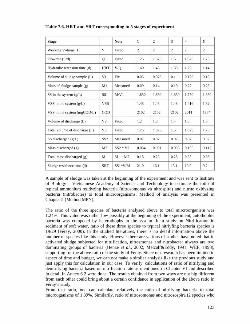
123

Table 7.6. HRT and SRT corresponding to 5 stages of experiment

Stage Note 1 2 3 4 5

Working Volume (L) V Fixed 2 2 2 2 2

Flowrate (L/d) Q Fixed 1.25 1.375 1.5 1.625 1.75

Hydraulic retension time (d) HRT V/Q 1.60 1.45 1.33 1.23 1.14

Volume of sludge sample (L) V1 Fix 0.05 0.075 0.1 0.125 0.15

Mass of sludge sample (g) M1 Measured 0.09 0.14 0.19 0.22 0.25

SS in the system (g/L) SS1 M/V1 1.850 1.850 1.850 1.770 1.650

VSS in the system (g/L) VSS 1.48 1.48 1.48 1.416 1.32

VSS in the system (mgCOD/L) COD 2102 2102 2102 2011 1874

Volume of discharge (L) V2 Fixed 1.2 1.3 1.4 1.5 1.6

Total volume of discharge (L) V3 Fixed 1.25 1.375 1.5 1.625 1.75

SS discharged (g/L) SS2 Measured 0.07 0.07 0.07 0.07 0.07

Mass discharged (g) M2 SS2 * V2 0.084 0.091 0.098 0.105 0.112

Total mass discharged (g) M M1 + M2 0.18 0.23 0.28 0.33 0.36

Sludge residence time (d) SRT SS1*V/M 21.0 16.1 13.1 10.9 9.2

A sample of sludge was taken at the beginning of the experiment and was sent to Institute of Biology – Vietnamese Academy of Science and Technology to estimate the ratio of typical ammonium oxidyzing bacteria (nitrosomonas và nitrospira) and nitrite oxidyzing bacteria (nitrobacter) to total microorganisms. Method of analysis was presented in Chapter 5 (Method MPN). The ratio of the three species of bacteria analysed above to total mircroorganism was 1.24%. This value was rather low possibly at the beginning of the experiment, autothophic bacteria was competed by heterothophs in the system. In a study on Nitrification in sediment of soft water, ratio of these three species to typical nitriyfing bacteria species is 19/29 (Féray, 2000). In the studied literatures, there is no detail information above the number of species like this study. However there are various of studies have noted that in activated sludge subjected for nitrification, nitrosmonas and nitrobacter always are two dominating groups of bacteria (Henze et al., 2002; Metcalf&Eddy, 1991; WEF, 1998), supporting for the above ratio of the study of Féray. Since our research has been limited in aspect of time and budget, we can not make a similar analysis like the previous study and just apply this for calculation in our case. To verify, calculations of ratio of nitrifying and denitrifying bacteria based on nitrification rate as mentioned in Chapter VI and described in detail in Annex 6.2 were done. The results obtained from two ways are not big different from each other could bring about a certain confidance in application of the above ratio in Féray’s study. From that ratio, one can calculate relatively the ratio of nitrifying bacteria to total microoganisms of 1.89%. Similarily, ratio of nitrosomonas and nitrosospira (2 species who

124

have greatest number of species among ammonium oxidyzing bacteria) to total microorganisms is 0.64 %. Ratio of two these species to total of ammonium oxidyzing bacteria is 15/22 (Féray, 2000). Relatively, one can calculate ratio of ammonium oxidyzing bacteria to total microorganisms of 0.93%. Ratio of nitrobacter (species who has the greatest number among nitrite oxidizing bacteria) to total microorganisms is 0.6%. Ratio of these species to total of nitrite oxidizing bacteria is 4/7 (Féray, 2000). Therefore, ratio of nitrite oxidizing bacteria to total microoganisms is 1.05%. Everyday, parameters including NH4

+, NO2- and NO3

- were analysed at the beginning of a new cycle (when leachate, NH4Cl and NaHCO3) were added (considered So) and at the end of old cycle (wastewater sample) (considered S).

7.2.3. Results Table 7.7 presents the results of analysis of the parameters. Values of each stage are average values taken at “steady state”

Table 7.7. Analysis results of the parameters obtained from kinetic and stoichiometric test

So (mg/L) S1 (mg/L) S2 (mg/L) S3 (mg/L) Stage NH4

+-N NH4+-N NO2

--N NO3--N

1 380 38.4 322.6 19.0 2 365 51 295.2 18.8 3 325 40.5 268.5 16.0 4 321 65 239.0 17.0 5 334 112 208.0 14.0

The average result of So and S ((So – S) as well) was calculated for each stage, together with correspoding HRT and SRT, concentration of nitrifying bacteria in the system. Based on that, recurrent equations were established and kinetic and stoichiometric parameters were calculated. Table 7.8 presents corresponding analysed values to establish recurrent equations (Graph 7.24) according to HRT for nitrifying bacteria. Table 7.8. Analysed values of nitrogen forms for establishment of recurrent equations based on HRT for nitrifying bacteria

θ (d)

So (mgN/L)

S (mgN/L)

X (mgCOD/L)

XA (mgCOD/L)

θX/(So-S) 1/S

θXA/(So-S) (d)

1.60 380 38.4 2102 41.6 9.844 0.026 0.195 1.45 365 51 2102 41.6 9.735 0.020 0.193 1.33 325 40.5 2102 41.6 9.849 0.025 0.195 1.23 321 65 2011 39.8 9.667 0.015 0.191 1.14 334 112 1874 37.1 9.649 0.009 0.191

125

Chart Title y = 0.2543x + 0.1882R2 = 0.9058

0.1900.1910.1920.1930.1940.1950.196

0.000 0.010 0.020 0.030

1/S (L/mg)

0XA

(So-

S)

(d)

0XA/(So-S) vs1/S

Linear (0XA/(So-S) vs 1/S)

Chart Title

y = 0.2361x - 0.0466R2 = 0.9951

0.0

0.1

0.1

0.2

0.2

0.0 0.5 1.0

(So-S)/0X

1/0

(So-S)/0X

Linear ((So-S)/0X)

Graph 7.24. Recurrent equations of kinetic parameters of activated sludge for nitrifying bacteria

Where θXA/(So-S) = 1/k + Ks/kS; we found values of kinetic parameters that are presented in Table 7.9.

Table 7.9. Kinetic parameters of activated sludge for nitrifying bacteria

1/k k Ks/k Ks 0.1882 5.314 0.254 1.35

Table 7.10. presents recurrent equations (Graph 7.25) according to SRT for nitrifying bacteria. Here, S is S1 in Table 7.7. Table 7.10. Analysed values of nitrogen forms for establishment of recurrent equations based on SRT for nitrifying bacteria

θc (d) So (mgN/L)

S (mgN/L)

X (mgCOD/L)

XA (mgCOD/L) 1/θ (So-S)/θX

20.96 380 38.4 2102 41.6 0.048 0.3916

16.10 365 51 2102 41.6 0.062 0.4686

13.07 325 40.5 2102 41.6 0.076 0.5229

10.85 321 65 2011 39.8 0.092 0.5926

9.18 334 112 1874 37.1 0.109 0.6516

Graph 7.25. Recurrent equations of kinetic and stoichiometric parameters of activated sludge for nitrifying bacteria

126

Chart Title y = 0.184x + 0.1389R2 = 0.9397

0.140

0.141

0.141

0.142

0.142

0.143

0.000 0.010 0.020

1/S (L/mg)

0XA

(So

-S)

(d)

0XA/(So-S) vs1/S

Linear (0XA/(So-S) vs 1/S)

Where 1/θc=Y.(So-S)/θX – kd; we found values of kinetic and stoichiometric parameters that are presented in Table 7.14 below:

Table 7.11. Kinetic and stoichiometric parameters of activated sludge for nitrifying bacteria

kd Y (mgCOD/mgN) µµµµm=k*Y 0.0466 0.236 1.25

Table 7.12. presents recurrent equations (Graph 7.26) according to HRT for ammonium oxidyzing bacteria. Value S (NO2

-) (mgN/L) in the Table was defined by substract value of NO3

- (S3) from S0 (Table 7.7). Table 7.12. Analysed values of nitrogen forms for establishment of recurrent equations based on HRT for ammonium oxidyzing bacteria

θ (d)

So (mgN/L)

S (mgN/L)

X (mgCOD/L)

XA_NH mgCOD/L) θX/(So-S) 1/S

θXA_NH/(So-S) (d)

1.60 380 57.4 2102 28.7 10.423 0.017 0.142 1.45 365 69.8 2102 28.7 10.355 0.014 0.141 1.33 325 56.5 2102 28.7 10.436 0.018 0.142 1.23 321 82.0 2011 27.4 10.355 0.012 0.141 1.14 334 126.0 1874 25.6 10.299 0.008 0.140

Graph 7.26. Recurrent equations of kinetic and stoichiometric paramters of activated sludge for ammonium oxidyzing bacteria

Where θXA/(So-S) = 1/k + Ks/kS; we found value of kinetic parameters of activated sludge for ammonium oxidizing that are presented in Table 7.13. Table 7.13. Kinetic parameters of activated sludge for ammonium oxidyzing bacteria

1/k k Ks/k Ks

0.1389 7.2 0.184 1.325 Table 7.14 presents corresponding analysed values to establish recurrent equations (Graph 7.27) according to SRT for ammonium oxidyzing bacteria.

127

Chart Title y = 0.1764x - 0.0489R2 = 0.9955

0.0

0.00.0

0.1

0.10.1

0.1

0.0 0.5 1.0

(So-S)/0X

1/0

(So-S)/0X

Linear ((So-S)/0X)

Table 7.14. Analysed values of nitrogen forms for establishment of recurrent equations based on SRT for ammonium oxidizing bacteria

θc (d) So (mg/L) S (mgN/L) X (mgCOD/L) XA_NH (mgCOD/L) 1/θ

(So-S)/θXA_NH

20.96 380 57.4 2102 28.7 0.048 0.5368 16.10 365 69.8 2102 28.7 0.062 0.6394 13.07 325 56.5 2102 28.7 0.076 0.7164 10.85 321 82.0 2011 27.4 0.092 0.8031 9.18 334 126.0 1874 25.6 0.109 0.8863

Graph 7.27. Recurrent equations of kinetic and stoichiometric parameters of activated sludge for ammonium oxidyzing bacteria

With 1/θc=Y.(So-S)/θX – kd; we found values of kinetic and stoichiometric parameters that are presented in Table 7.15. Table 7.15. Kinetic and stoichiometric parameters of activated sludge for ammonium oxidyzing bacteria

kd Y (mgCOD/mgN) µµµµm=k*Y 0.0489 0.176 1.27

For kinetic and stoichiometric parameters of nitrite oxidizing bacteria, it is not easy to determine in the same way of what done for nitrifying bacteria and ammonium oxidizing bacteria. Although we can still determine total nitrogen of nitrite produced after process (cycle of day) as well as nitrite oxidized to nitrate. However, the amount of nitrite can not be considered as equal to the initial concentration (S0) since it changes very much during the whole experiments), while the amount of nitrate produced at the end of the cycle is usually not high which would yield large errors in the estimation. Relatively, the yield coefficient of nitrite oxidizing bacteria in this case will be taken equal to the difference between whole process of nitrification (ammonium oxidizing bacteria) and the one of nitrifying bacteria and. Y_A_NO2 = 0.236 – 0.176 = 0.06 We can calculate relatively the maximum growth rate of nitrite oxidizing bacteria is equal to the product of that of ammonium oxidizing bacteria and ratio of nitrate to nitrite produced. µm_XA_NO2 = µm_XA_NH * 0.07 = 1.27 * 0.07 = 0.081 d-1.

128

Parameters of heterothoph microorganisms can not be determined in this test because organic matters just decreased after short time (at the beginning of the period about 8 first days), but not further. This result possibly due to the following phenomena:

- Degradation of slowly biodegradable COD (X_S) in the inlet leachate into easily biodegradable COD (S_S);

- Decay of biomass in the system; - COD stored in biomass (X_STO) and then freed during the decay of biomass.

The general result and the reference data from literatures are given in the Table 7.16 below:

Table 7.16. Kinetic and stoichiometric parameters of the studying activated sludge

This study (at 27.5 oC) Refrence (Henze et al., 2002) at 20oC

Unit X_A_NH X_A_NO2 Overall X_A_NH X_A_NO2 Overall

Ks mgN/L 1.32 - 1.35 0.3 – 0.7 0.8 – 1.2 0.3 – 0.7

Y mgCOD/mgN

0.176 0.06 0.236 0.1 – 0.12* 0.05 – 0.07* 0.15 – 0.2*

µm d-1 1.270 0.081 1.255 0.6 – 0.8 0.6 – 1.0 0.6 – 0.8

kd d-1 0.0489 - 0.047 0.03 – 0.06 0.03 – 0.06 0.03- 0.06

* (mgVSS/mgNO3-N formed) According to (Henze et al., 2002), maximum growth rate of bacteria at present temperature can be determined from values at 20oC with Equation 7.1. µm(ToC) = µm(20oC). exp(κ(T-20)) (Eq. 7.1) Where κ is the temperature factor for µm and bA, which has an average value of 0.1 o C-1 for ammonium oxidizing bacteria. The experiment was implemented in the average temperature of 27.5oC, the maximum growth rate ammonium oxidizing bacteria determined according to the Eq. 7.1 (taking value of µmA_NH (20oC) of 0.6 d-1 (Henze et al., 2002)) is 1.28 d-1. The result obtained from our experiment is 1.27 d-1 that is very close to the literature value. There was not temperature control on the pilot, therefore temperature in the lab during experiment has changed. At the beginning of the calibration period, temperature was low, around 16.8 oC (average), and increased up to 25.4 oC at the end of calibration. Temperature used for calculus is the average, which is 20.2 oC. Maximum growth rate of ammonium oxidizing bacteria determined according to the Eq. 7.1. is 0.61 d-1. Decay constant bA of ammonium oxidizing bacteria is determined based on kd coefficient according to Eq. 7.2 (Tabares, 2006) :

)I_X_f1(Y1

kdb

AA −−

= (Eq. 7.2)

Where f-X_I is production of X_I (inert particulate products) in aeration endogenous respiration. Taking the defaut value of 0.2 in the ASM 3 model, we get bA equal to 0.0628 d-1. The literature value of bA at 20oC is 0.03 d-1, the experimental bA at 20.2oC therefore is 0.03 d-1 . The values of main parameters (µ) obtained from our experiment at temperature of 20oC in are the range of literature values except the Ks of ammonium oxidizing bacteria

129

which is a little bit greater. However, the difference will not cause significant errors since input concentration of ammonium (considered as S) used for calibration is much higher than KS. Maximum growth rate of nitrite oxidizing bacteria is much smaller than those from literature. To our opinion this is due to the influence of high pH and high concentration of alkalinity that will be discussed in the Chapter 8. In the validation time, spring has caused a significant increase of temperature, which averaged at 24.98oC. µmA_NH and bA (for both AOB và NOB) determined for this period are 0.987 d-1 and 0.049 d-1, respectively.

7.3. RESPIRATION TEST (FOR DETERMINATION OF HETEROT ROPHIC YIELD (YH) The ratio of the amount of biomass produced to the amount of substrate consumed (mg biomass/mg substrate) is defined as the biomass yield, and is typically defined in relation to the electron donor used. In the case of heterotrophic microorganisms, their yield (YH) is the amount of heterotrophic biomass produced to the amount of biodegradable organic matter (S) consumed. As presented in Figure 7.2, from a unit of subtrate consumed the YH fraction goes to biomass growth and the rest (1-YH) is used for respiration. Thus, the yield coefficient can also be related to the DO consumption of the heterotrophic organisms under particular conditions and this consumed DO can be measured by using a respiromenter.

)COD_(consumed_emgsubstrat

)COD_(produced_mgbiomasYwthBiomassgro H= (Eq. 7.3)

)COD_(consumed_emgsubstrat

consumed_mgO)Y1(spirationRe 2

H−= (Eq. 7.4)

Figure 7.2. Description of the substrate transformation for the biomass growth and the biomass respiration (Tabares, 2006).

Equation. 7.3 and 7.4 describes how adding substrate to the sludge represents an oxygen consumption. The slope of this function corresponds to the factor (1-YH). In these respirometric essays, the quantity of DO consumed is measured for each quantity of substrate added to the sludge sample yielding different values of the consumed DO/substrate relationship. The graphical representation of the pairs of values obtained in the different additions is linear with a slope (1-YH). Preparation:

- A closed tank with a 500 ml, volume, with a small straw for sampling, a hole to install DO probe, a small hole to inject ATU as inhibitor of nitrification.

- Endogenous activated sludge is separated into 5 aliquots. Those aliquots are spilled to the 500 ml tank with leachate and clean water to reach a volume of 500 ml and aVSS concentration of 2.25 g/L.

- Leachate (NH4+ = 296 mgN/L, COD = 420 mgO2/L): is divided into 5 50 ml parts,

volume. After dilution in the 500 ml reactor NH4+ and COD concentrations are

S

YH

1-YH

130

Test for Y_H determination

y = -1.9958x + 7.6515

R2 = 0.9754

y = -1.6883x + 7.6709

R2 = 0.9759

y = -2.3199x + 7.6679

R2 = 0.9954

y = -4.7508x + 7.6219

R2 = 0.9889

y = -2.7552x + 7.6598

R2 = 0.9896.6

6.8

7

7.2

7.4

7.6

7.8

0 0.05 0.1 0.15 0.2

Time (h)

OU

R_C

OD

(m

gO2/

L.h)

Test 1Test 2Test 3Test 4Test 5Linear (Test 2)

14.8 mgN/L and 21 mgO2/L, respectively. This COD, however, is mostly inert COD.

- Solution of sugar (C12H22O11 with COD of 1.12 mgO2/mg: is prepared with COD of 10000 mgO2/L.

- Nitrifying bacteria inhibitor (ATU) (5mg/L) (State, 2004).

Test implementation: 5 tests were implemented (from test 1 to test 5) with various volumes of sugar solution (diluted from the 10000 mg O2/L solution), as shown showed in Table 7.17.

Table 7.17. COD addition in the tests for determination of YH

Test Volume of sugar solution (mL) Weight of sugar (mg COD) 1 1 10 2 1.5 15 3 2 20 4 2.5 25 5 3 30

Spill the activated sludge into the 500 ml tank, then spill 50 ml leachate into the tank to creat base environment, then dilute with clean water to 500 mL, then inject some drops of ATU, then add the 10000 mg O2/L sugar solution with different volume corresponding to each test to the tank; When the final dilution is done the tank is covered and aerated. DO is recorded during in the whole process (0.2 hours). The DO decrease yields the oxygen uptake rate (OUR) of heterotroph bacteria corresponding to the various COD concentrations (Graph 7.28).

Graph 7.28. OUR_COD for various COD concentrations.

131

Test for Y_H determination

y = 0.3167x - 7.7181

R2 = 0.9343

0

1

2

3

4

5

25.0 30.0 35.0 40.0

(S0-S1) (mgCOD/L.h)

OU

R_C

OD

(m

gO2/

L.h)

Series1

Linear (Series1)

Table 7.18. Data analysis of the OUR tests

Test No OUR_COD (mgO2/L.h)

S0 (mgCOD/L)

S1 (mgCOD/L) (after 0.2h)

(S0-S1) (mgCOD/L.h)

Biomass activity (mg/gVSS.L.h)

1 1.6883 31.7 26 28.5 12.7 2 1.9958 39 32.7 31.5 14.0 3 2.3199 52 45.6 32.0 14.2 4 2.7552 67.6 60.8 34.0 15.1 5 4.7508 89 81.3 38.5 17.1

Graph 7.29. Y_H determination based on OUR

From Figure 7.29 the slope (i.e equal to 1-YH ) is equal to 0.3167 yielding a YH of 0.6833.

132

REFERENCES

1. Féray, C., 2000, Nitrification en sédiment d'eau douce : incidence de rejets de station d'épuration sur la dynamique de communautés nitrifiantes, Université Lyon I, France., 204 p.

2. Henze, M., P. Harremoes, J. L. C. Jansen, and E. Arvin, 2002, Wastewater Treatment: Biological and Chemical Processes: ISBN 3-540-42228-5, Springer - Verlag Berlin Heidelberg, Germany.

3. Metcalf&Eddy, 1991, Wastewater Engineering. Treatment, Disposal and Reuse: New York, Mc Graw - Hill Book Company. , 1771 p.

4. State, P., 2004, Institutes of the Environment Annual Technical Report FY 2004, p. 49.

5. Tabares, L. C., 2006, Control and optimization of an SBR for nitrogen removal: From model calibration to plant operation, Universitat de Girona, Girona, 231 p.

6. WEF, 1998, Biological and chemical systems for nutrient removal, Alexandria, USA.

133

CHAPTER VIII

APLICATION OF DATA ANALYSIS AND EXPERIMENTAL PLANNING METHOD TO STUDY PARTIAL

NITRIFICATION

8.1. MATERIALS

8.1.1. Leachate and activated sludge Leachate used for experimental batches were collected at Nam Son landfill site, Hanoi. Average characteristics of the leachates used during the study (15/10-15/11/2008) are given in Table 8.1. Table 8.1. Leachate characteristics in Nam Son landfill site during the study (a from biological ponds b at collection ponds).

Components Unit Value

NH4+ mgN/L 57.5a - 425b

NO2- mgN/L 0.01

NO3- mgN/L 0.01

TKN mgN/L 127a - 358b

COD mgO2/L 230a - 555b

BOD mgO2/L 35a - 56b

Alkalinity mg/CaCO3L 1100a - 2880b

PO43- mgP/L 3.4a - 6.8b

pH - 8.5 - 8.8

8.1.2. Activated sludge Activated sludge was collected at the Domestic WWTP Kim Lien – Truc Bach, Hanoi. This sludge was continuously aerated and fed with leachate, NH4Cl and alkalinity

Summary: This chapter presents a study on partial nitrification by applying data analysis and experimental planning method. This work is also the content of a paper that has been presented in the Twelfth International Waste Management and Landfill Symposium, Sardinia, October 2009. It consists of “Materials”, “Data analysis and planning of experiments”, “Results and discussions” and “Conclusions”. The most important parts in “Results and discussion” is observations and discussions in “Ammonium uptake rate, nitrite production rate, nitrate production rate, biomass activity and NO2/(NO2+NO3) ratio” and “Data analysis and establishment of recurrent equations of influencing factors”.

134

(NaHCO3) during two months, has shown a good ammonium removal activity. Sludge age and biomass concentration were kept stable during experimental batches respectively 10 day and 2.5 g MLSS/L (~ 2 gMLVSS/L).

8.1.3. Chemicals NH4Cl and NaHCO3 were added to the leachate to ensure the concentration of ammonium following the planning of experiment. KHPO4 was sometimes added to the system in case of insufficiency of phosphor for biomass growth.

8.14. Single reactor Single reactor is a 3L tank (30cm x 20 cm x 10 cm), working volume of 2.5L, installed with aerator and mixer. Working time of nitrification phase was 6 hours.

8.1.5 Online measurement DO probe (Oxi 197i – WTW).

8.2. DATA ANALYSIS AND PLANNING OF EXPERIMENTS Planning of experiments is a procedure to select the necessary and sufficient experimental conditions number of experiments, to achieve objectives with a fixed accuracy; and is also the selection of mathematical methods to treat experimental results and to concede those results (Himmelblau, 1970; Pham and Ngo, 2007) . In this study, planning of experiment with first-order full factors is used to study nitrification. The experiments are planned as follows: - Number of factor k: 3, including inlet concentration of NH4

+ (mgN/L), alkalinity (mgCaCO3/L) and aeration rate (corresponding to the Kla value). - Number of level n: 2, including two values of the factors, typically highest value and typically lowest value of concentration of NH4

+ (mgN/L) (e.g. 400 and 100 respectively) and alkalinity (mgCaCO3/L) (e.g. 3400 and 1150 respectively) of the studied leachate, and two levels of aeration rate with Kla’ (in system with biomass) are 18.35 and 10.89 h-1 respectively to keep DO concentration in the system around 2-3 mg/L and 0.5-1.5 mg/L, respectively. This range of DO concentration is selected because it is favourable for nitrite accumulation of 85% to 98% (Ciudad et al., 2005; Jianlong and Jing, 2005; Pambrun et al., 2004; Ruiz et al., 2002). The experiments for determination of maximum nitrification and denitrification capacity implemented with the highest DO supply intensity of this experiment (Kla’ = 18.35 h-1) in Chapter 7 also obtained high nitrite accumulation (84 - 94%). A lower intensity of DO supply (Kla’ = 10.89 h-1) therefore is applied in this experiment to see if we can save more energy while keeping a good enough nitrogen removal efficiency. - Number of experimental batch N = nk = 23 = 8. Each experimental batch was repeated three times. - Temperature during experiments was 26 to 28oC. Matrix of experimental batches is given in Table 8.2.

135

Table 8.2. Matrix of experimental batches

NH4

+ Alkali-nity

DO

Values in coordinates

AUR

NPR

1

NPR

2

BA

NO2/ (NO2+ NO3)

mgN/L.h

mgN/L.h

mgN/L.h

mgN/ gVSS

.h

-

Batch

mgN/L

mg CaCO

3/L

Kla (h-1)

x0

x1 x2 x3 x1x2

X1x3

x2x3

x1x2x3

Y1 Y2 Y3 Y4 Y5

1 100 1150 10.89 1 -1 -1 -1 1 1 1 -1

2 400 1150 10.89 1 1 -1 -1 -1 -1 1 1

3 100 3400 10.89 1 -1 1 -1 -1 1 -1 1

4 400 3400 10.89 1 1 1 -1 1 -1 -1 -1

5 100 1150 18.35 1 -1 -1 1 1 -1 -1 1

6 400 1150 18.35 1 1 -1 1 -1 1 -1 -1

7 100 3400 18.35 1 -1 1 1 -1 -1 1 -1

8 400 3400 18.35 1 1 1 1 1 1 1 1

A matrix of experimental planning between the products of nitrification process and

nitrite accumulation, which are influenced by input factors, is established. Because the number of experimental batches is 8, the number of coefficients in the recurrent equation is equal or less than 7, then we remove the third-order interaction coefficient (b1b2b3). The general recurrent equation can be written as follows: y = b0 + b1x1 + b2x2 + b3x3 + b12x1x2 + b13x1x3 + b23x2x3 (Eq. 8.1)

Coefficients and their signification according to the Student standard are given. The

recurrent equation will be established after removal of non-significant coefficients. Finally, experimental suitability of this equation will be verified in accordance with Fisher standard (Akhnazarova and Kafarov, 1978; Himmebblau, 1970; Pham and Ngo, 2007).

8.3. RESULTS AND DISCUSSIONS

8.3.1. Tracer test to determine mixing capability of the system The test was implemented in the reactor during fill-aeration (at lowest speed with Kla of 10.89 h-1). Temperature was about 23.2oC. An amount of NaCl (100 g.l-) was injected into the reactor. Variation of conductivity was recorded yielding the time needed for the system to reach 95% of the final value of conductivity.

136

Conductivity versus time

0

20

40

60

80

100

120

140

160

40 50 60 70 80 90 100 110 120 130 140 150 160 170 180

Time (s)

Con

duct

ivity

(m

S/c

m)

14 s

Graph 8.1. Tracer test to determine the mixing time

With the initial value of 20 and 146.3 µS/cm, time needed for the system to get 95 % of stable value (139 µs/cm) is 14 seconds, which is very small compared to the 6 hours of the whole nitrification process. It can be concluded that the system is well mixed.

8.3.2. Gas-liquid mass transfer coefficients Kla Gas-liquid mass transfer coefficient in the system with presence of biomass (Kla’) was determined in the reactor aerated with different (airflow rates), including the lowest and highest speeds (airflow rates) as mentioned in item 8.2 and 3 intermediate values. The speed of aeration (airflow rates) is controlled by a valve. With the Kla’values, the oxygenation capacity (OC’) and the standard oxygen transfer rate (SOTR’) are determined. The values are given in Table 8.3. The procedure is similar to the one described in more details in chapter VI.

Table 8.3 Kla and other parameters of the single reactor

Kla’ Cs’ OC’ SOTR’ Aeration

speed h-1 mgO2/L mgO2/Lh mgO2/h A 18.4 8.15 149 374 B 10.9 7.77 85 211 C 15.7 8.03 126 316 D 15.1 7.98 120 301 E 15.2 7.89 120 300

Kla value that is approximate the average value of Kla values at lowest and highest aeration speed will be chosen for central experimental batch. Here, it is 15.1 h-1. OC’ and SOTR’ values will be compared with respiration rate of biomass in experimental batches. From this, it will be concluded either if the system is sufficiently supplied in oxygen for biomass growth in the whole process.

137

Respiration rate during NitrificationBatch 1

-70

-50

-30

-10

10

30

50

0.0 0.5 1.0 1.5 2.0 2.5 3.0 3.5 4.0 4.5 5.0 5.5 6.0

Time (h)

RO

(mgO

2/L.

h)

0

1

2

3

4

5

6

7

8

9

RO

DO

DO

(mg/

L)

Respiration rate during NitrificationBatch 2

-80

-60

-40

-20

0

20

40

60

80

0.0 0.5 1.0 1.5 2.0 2.5 3.0 3.5 4.0 4.5 5.0 5.5 6.0

Time (h)

RO

(mgO

2/h)

0

1

2

3

4

5

6

RO

DO

DO

(mg/

L)

8.3.3. Respiration rate of biomass With the Kla’ values from Table 4.1, respiration rate (Ro) of the biomass in the system is calculated with the following formula (at filling gas – static liquid state): Ro = Kla’ (S*o-So) – dSo/dt (Spanjers and Vanrolleghem, 1995). (Eq. 8.2) The respiration rates at steady state of the experimental batches are given in Table 8.4: Table 8.4. The respiration rate at steady state

At steady state

Batch Ro (mgO2/L.h) Ro (mgO2/h) Ro (mgO2/gVSS.h) DO (mgO2 /L) 1 74.8 187 37.4 0.90 2 79.3 198 39.6 0.49 3 71.5 179 35.8 1.22 4 75.2 188 36.4 0.86 5 109.7 274 54.8 3.08 6 124.4 311 62.2 1.37 7 112.5 281 56.3 2.02 8 120.2 300 60.1 1.60

Centre 97.9 245 48.9 1.49 Table 8.4 shows that, the respiration rate of biomass is directly proportional to aeration intensity or DO concentration in the liquid. Ro from Batch 1 to 4 (lowest aeration) are very different from each other (71.5 – 79.3 mgO2/L.h), and the same with Ro from Batch 5 to 8 (109.7 -124.4 mgO2/L.h). Ro of Central Batch is 97.9 mgO2/L.h, approximates the average Ro value at lowest and highest aeration speed. By the way, comparing the Ro values with OC’ (oxygen concentration presents in the liquid) in Table 8.3, it is shown that, the aeration intensity of all experimental batches are high enough to supply the biomass with oxygen sufficiently, particularly during steady state. The RO and DO evolution are also presented in Graphs 8.2 - 8.10. The curve of RO in the graph was smoothed by Savitsky - Golay Filters method (Savitsky and Golay, 1964). An example of calculation is found in Annex 6.1.

138

Respiration rate during NitrificationBatch 3

-60

-40

-20

0

20

40

60

0.0 0.5 1.0 1.5 2.0 2.5 3.0 3.5 4.0 4.5 5.0 5.5 6.0

Time (h)

RO

(mgO

2/h)

01

23

45

67

89

RO

DO

DO

(mg/

L)

Respiration rate during NitrificationBatch 4

-60

-40

-20

0

20

40

60

0.0 0.5 1.0 1.5 2.0 2.5 3.0 3.5 4.0 4.5 5.0 5.5 6.0

Time (h)

RO

(mgO

2/h)

0

0.5

1

1.5

2

2.5

3

3.5

4

RO

DO

DO

(mg/

L)

Respiration rate during NitrificationBatch 5

-120

-90

-60

-30

0

30

60

0.0 0.5 1.0 1.5 2.0 2.5 3.0 3.5 4.0 4.5 5.0 5.5 6.0

Time (h)

RO

(mgO

2/Lh

)

0

1

2

3

4

5

6

7

8

9

RO

DO

DO

(mg/

L)

Respiration rate during NitrificationBatch 6

-120

-90

-60

-30

0

30

60

90

120

0.0 0.5 1.0 1.5 2.0 2.5 3.0 3.5 4.0 4.5 5.0 5.5 6.0

Time (h)

RO

(mgO

2/L.

h)

0

1

2

3

4

5

6

7

8

9

RO

DO

DO

(mg/

L)

Respiration rate during NitrificationBatch 7

-120

-90

-60

-30

0

30

60

90

0.0 0.5 1.0 1.5 2.0 2.5 3.0 3.5 4.0 4.5 5.0 5.5

Time (h)

RO

(mgO

2/h)

0

1

2

3

4

5

6

7

8

9

RO

DO

DO

(m

g/L)

Respiration rate during NitrificationBatch 8

-120

-90

-60

-30

0

30

60

90

120

0.0 0.5 1.0 1.5 2.0 2.5 3.0 3.5 4.0 4.5 5.0 5.5 6.0

Time (h)

RO

(mgO

2/L.

h)

0

1

2

3

4

5

6

7

8

9

RO

DO

DO

(mg/

L)

Respiration rate during NitrificationBatch Central

-100

-70

-40

-10

20

50

80

0.0 0.5 1.0 1.5 2.0 2.5 3.0 3.5 4.0 4.5 5.0 5.5 6.0

Time (h)

RO

(mgO

2/L.

h)

0

1

2

3

4

5

6

7

8

9

RO

DO

DO

(mg/

L)

Graphs 8.2 - 8.10. Ro and DO evolution in Nitrification from Batch 1 - 8 and Central Batch.

139

8.3.4. Ammonium uptake rate (AUR), nitrite production rate (NPR1), nitrate production rate (NPR2), biomass activity (BA) and NO2-/(NO2-+NO3-) ratio The results of the experiments with focus on AUR, NPR1, NPR2, BA and NO2

-/(NO2-

+NO3-) ratio are presented in Table 8.5. Values given in the table are average on three

repeated experiments. Process time is 6 hours; samples were taken each hour. AUR, NPR1 and NPR2 are coefficients “a” of linear recurrent equations y = ax + b. That means, for the Batches with lowest concentration of input ammonium of 100 mgN/L (1, 3, 5, 7), AUR and NPR1 are calculated during the time from the beginning to the hour when ammonium was consumed completely or nearly completely (~ 5mg/L). NPR2 was calculated for the whole process (6 hours) because even when ammonium had been consumed, nitrate production was still taking place due to nitrite oxidation. BA (mgN/gVSS.h) is the ratio of AUR and VSS. NO2

-/(NO2-+NO3

-) is the ratio of NPR1 and (NPR1+NP2) for Batches 2, 4, 6, 8 and ratio of difference of NO2

- at the beginning and the end and that of (NO2-+NO3

-) for Batches 1, 3, 5, 7. Time for the whole process therefore is also considered as an auxiliary influence. Table 8.5. Results of Nitrification process of experimental batches

AUR NPR1 NPR2 Biomass activity NO2/(NO2+NO3)

Batch NH4-Alk-DO

mgN/L.h mgN/L.h mgN/L.h mgN/gVSS.h

Batch1 100-1150-B 21.2 19.8 2.02 10.6 0.892 Batch2 400-1150-B 23.5 21.1 1.90 11.8 0.917 Batch3 100-3500-B 21.6 19.3 1.46 10.8 0.907 Batch4 400-3500-B 24.0 21.7 1.66 12.0 0.929 Batch5 100-1150-A 29.5 26.8 2.70 14.7 0.830 Batch6 400-1150-A 36.3 34.0 2.64 18.1 0.928 Batch7 100-3500-A 32.3 30.8 2.26 16.1 0.866 Batch8 400-3500-A 38.7 35.9 1.97 19.3 0.948

Batch centre 250-2400-C 30.4 27.2 2.29 15.2 0.922

AUR: AURs of Batches 1-4 (Kla = 10.9 h-1) are a little bit different from each other (21.2 – 24.0 mgN/L.h), when [NH4

+] changes. The alkalinity also shows a light influence for batches with a same [NH4

+]. AUR is greater when [NH4+] and alkalinity are higher.

For the Batches 5-8, (Kla = 18.4 h-1), AUR values (29.5-38.7 mgN/L.h) are higher with larger differences between experiments especially when [NH4

+] varies. The influence of alkalinity here is also more significant. NPR1: NPR1’s evolution is similar with AUR’s. The influence of alkalinity, however, is only significant in the Batches with the highest Kla. Here, there is also an interaction between input factors. NPR2: NPR2s from Batch 1 to 8 do not change very much in comparison with NPR1s. The highest NPR2 (2.7 mgN/L) is obtained in Batch 5. This is reasonable since the input [NH4

+] and alkalinity are lowest, while oxygen is supplied at highest level. However, it should be noted that, here, nitrate is produced in the whole process. In fact, alkalinity (HCO3

-) only plays a secondary role, participating to the process as a buffer of the water environment, preventing the pH to decrease caused by H+ production during ammonium oxidation. The one who has the main influence is neutralized NH3, which is a inhibitor for nitrite oxidizing bacteria at concentration of NH4

+ of 2-20 mgN/L when pH > 8.0 and of 7-70 mgN/L when pH > 7.5 (Anthonisen et al., 1976). In addition, NH3 is directly proportional to pH (Eq. 4.1) (Metcalf&Eddy, 1991).

140

Batch 1_1 y = 1.9125x - 0.6571R2 = 0.9642

y = -20.843x + 121.63R2 = 0.9802

y = 20.393x - 14.833R2 = 0.9797

-20

0

20

40

60

80

100

120

0h 1h 2h 3h 4h 5h 6h

Time (hour)

N (

mgN

/L)

0

200

400

600

800

1000

1200

NO2

NH4

NO3

NO2+NO3

Alkalinity

Alk

alin

ity

(mgC

aCO

3/L )

Batch 2_3y = -23.089x + 426.43R2 = 0.9747

y = 20.263x - 21.95R2 = 0.9962

y = 1.9571x - 2.7857R2 = 0.9595

-100

0

100

200

300

400

500

0h 1h 2h 3h 4h 5h 6h

Time (hour)

N (

mgN

/L)

0

200

400

600

800

1000

1200

1400

NO2NH4NO3NO2+NO3Alkalinity

Alk

alin

ity

(mgC

aCO

3/L)

NH4 ↔ NH3 (pH= 9.2) (Eq. 8.3) pH values measured during 6 hours of nitrification from Batch 1 to 8 are in the range of 7.96 - 9.4, typically 8.5 – 8.7. pH less than 8 is rarely observed and only in the Batches with lowest alkalinity ; particularly in Batch 6, pH from the third hour rapidly decreased, reaching 6.28 in the last hour. It is because alkalinity in this case is consumed almost completely, buffer capacity of the system decreased strongly while nitrification was taking place. This causes a pH decrease but the inhibition effect of NH3 on nitrite oxidizing bacteria also decreased. Therefore, nitrite is continuously oxidized into nitrate during the last hours of this experiment. Biomass activity: Biomass in the system was kept stable, close to 2 gVSS/L. BA is calculated from AUR, so its variation is the same than for AUR. NO2

-/(NO2-+NO3

-): This ratio depends on NPR1 and NPR2. However, the ratio itself plays a decisive role. Because the NPR2s of the batches are much smaller than NPR1s, therefore the ratio depends mostly on NPR1s. Batch 8 has the highest ratio (0.948) due to a combination of high ammonium and alkalinity, even with highest DO. Batch 4, with the highest ammonium and alkalinity and the lowest DO, should achieve the highest NO2

-

/(NO2-+NO3

-) but its ratio remains smaller than for Batch 8. It is because the low aeration rate induces smaller AUR and NPR1. Reasonably, Batch 5 with conditions that are favourable for nitrite oxidizing bacteria yields the smallest ratio of nitrite accumulation (0.830). There is a notable tendency on NO2

-/(NO2-+NO3

-) ratio from batch to batch. This ratio is higher in the Batches with highest concentration of ammonium than the others (0.917-0.948 compared with 0.830-0.907); and also with highest alkalinity. Influence of aeration rate is less obvious in this case. Nitrification process with NO2

-, NO3-, Alkalinity evolution of Batch 1 – 8 and Batch Centre is

also given in the graphs bellows:

141

Batch 5_3 y = 2.9786x - 3.3714R2 = 0.972

y = -24.22x + 115.54R2 = 0.9822

y = 22.046x - 14.152R2 = 0.9824

-20

0

20

40

60

80

100

120

0h 1h 2h 3h 4h 5h 6h

Time (hour)

N (

mgN

/L)

0

200

400

600

800

1000

1200

1400

NO2

NH4

NO3

NO2+NO3

Alkalinity

Alk

alin

ity

(mgC

aCO

3/L)

Batch 6_2 y = 2.9946x - 3.5R2 = 0.9682

y = -36.482x + 427.36R2 = 0.9833

y = 33.157x - 32.101R2 = 0.9963

-100

0

100

200

300

400

500

0h 1h 2h 3h 4h 5h 6h

Time (hour)

N (

mgN

/L)

0

200

400

600

800

1000

1200

1400

NO2

NH4

NO3

NO2+NO3

Alkalinity

Alk

alin

ity

(mgC

aCO

3/L)

Batch 8_2 y = 1.6821x - 1.1286R2 = 0.9662

y = -37.375x + 429R2 = 0.9786

y = 34.289x - 33.829R2 = 0.979

0

100

200

300

400

500

0h 1h 2h 3h 4h 5h 6h

Time (hour)

N (

mgN

/L)

0

1000

2000

3000

4000

NO2

NH4

NO3

NO2+NO3

Alkalinity

Alk

alin

ity

(mgC

aCO

3/L )

BatchCentral y = 27.341x - 20.446

R2 = 0.9901y = -31.625x + 245.79

R2 = 0.9806y = 2.4946x - 0.8286

R2 = 0.9427

0

50

100

150

200

250

0 1 2 3 4 5 6 7 8

Time (h)

NH

4/N

O2/

NO

3/N

O2+

NO

3 (m

gN/L

)

0

500

1000

1500

2000

2500

Alk

alin

ity (

mgC

aCO

3/L)

NH4

NO2

NO3

NO2+NO3

Alkalinity

Linear

Batch 3_3 y = 1.3107x - 0.8643R2 = 0.9759

y = -20.526x + 115.92R2 = 0.975

y = 18.657x - 17.933R2 = 0.9981

-20

0

20

40

60

80

100

120

0h 1h 2h 3h 4h 5h 6h

Time (hour)

N (

mgN

/L)

0

500

1000

1500

2000

2500

3000

3500

NO2

NH4

NO3

NO2+NO3

Alkalinity

Alk

alin

ity

(mgC

aCO

3/L)

Batch 4_1 y = 1.4204x - 1.9657R2 = 0.9536

y = -22.75x + 435.36R2 = 0.983

y = 19.185x - 22.716R2 = 0.9789

-100

0

100

200

300

400

500

0h 1h 2h 3h 4h 5h 6h

Time (hour)

N (

mgN

/L)

0

1000

2000

3000

4000

NO2

NH4

NO3

NO2+NO3

Alkalinity

Alk

alin

ity

(mgC

aCO

3 /L)

Batch 7_3 y = 2.2339x - 1.2357R2 = 0.967

y = 31.825x - 29.2R2 = 0.9996

y = -34.442x + 132.45R2 = 0.9713

-50

0

50

100

150

200

250

0h 1h 2h 3h 4h 5h 6h

Time (hour)

N (

mgN

/L)

3000

3200

3400

3600

3800

4000

NO2

NH4

NO3

NO2+NO3

Alkalinity

Alk

alin

ity

(mgC

aCO

3/L)

Graphs 8.11 – 8.19. Nitrification evolution in Batch 1 – 8 and Batch Centre.

142

DO, pH, ORP (To) versus time Batch 2

0

2

4

6

8

10

0 1 2 3 4 5 6

Time (h)

DO

(m

g/L)

-10

1030

50

70

90110

130

150

OR

P (

mV

) T

o (o

C)

DO

pH

To

ORP

DO, pH, ORP and To versus time Batch 3

0123456789

10

0 1 2 3 4 5 6

Time (h)

DO

(m

g/L

), p

H

-20

0

20

40

60

80

100

120T

o (o

C),

OP

R (

mV

)

DO

pH

To

ORP

DO, pH, ORP and To versus time Batch 1

0

2

4

6

8

10

0 1 2 3 4 5 6

Time (h)

DO

(m

g/L)

/pH

-50-30-101030507090110130

To (

oC)/O

RP

(mV

)

DO

pH

To

ORP

DO, pH, ORP and To versus time Batch 4

0123456789

10

0 1 2 3 4 5 6

Time (h)

DO

(mg/

L)/p

H

-20-100102030405060708090100110120130

To (o

C)/O

RP

(mV

)

DO

pH

To

ORP

DO, pH, ORP and To versus time Bacth 5

012345

6789

10

0 1 2 3 4 5 6

Time (h)

DO

(m

g/L)

0

20

40

60

80

100

120

140

To

(oC

), O

RP

(m

V)

DO

pH

To

ORP

DO, pH, ORP and To versus time Batch6

0123456789

0 2 4 6Time (h)

DO

(m

g/L)

/pH

0

50

100

150

200

To

(oC

)/O

RP

(mV

)

DO

pH

To

ORP

DO, pH, ORP and To versus time Bacth 7

0

2

4

6

8

10

0 1 2 3 4 5 6

Time (mg/L)

DO

(m

g/L)

-20020406080100120140160

DO

pH

To

ORP

DO, pH, ORP and To versus time Batch 8

0123456789

10

0 1 2 3 4 5 6

Time (h)

DO

(m

g/L)

, pH

0

20

40

60

80

100

120

To

(oC

), O

RP

(m

V)

DO

pH

To

ORP

DO, ORP, pH and temperature

143

DO and To versus time Batch Central

0

2

4

6

8

10

0 1 2 3 4 5 6

Time (h)

DO

(m

g/L)

, pH

0

20

40

60

80

100

120

140

160

To

(oC

), O

RP

(m

V)

DO

pH

To

ORP

Graphs 8.20 – 8.28. DO, pH, ORP evolution during nitrification process in Batch 1 – 8 and Batch Centre.

8.3.5. Data analysis and establishment of recurrent equations of influencing factors Data are processed in Excel and HAIKHH software. In each experiment corresponding to a row in Table 8.2, we determine the average values of factors according to m (i.e. 3 in this case) of repeated experiments and their variance:

N,...2,1i,1m

)yy(

s

m

1u

2iiu

2i =

−

−

=∑

= (Eq. 8.4)

Homogeneity of the variances is verified by Cochran standard;

∑=

=N

1i

2i

2max

s

sG (Eq. 8.5)

Comparing with values of Cochran distribution in Persentile Table G1-p(n,f) with p = 0.05, n = N = 8, f = m - 1 = 2; G0.05(8,2) is 0.517, all G values obtained according to (Eq. 8.15) are smaller than 0.517, then the variances are homogeneous. Regenerate variance is determined through average variance:

N

s

s

N

1i

2i

2ts

∑== (Eq. 8.6)

Coefficients of recurrent equations are determined according to Equation 5.3. The variance of coefficients is determined by the following equation:

m.N

ss

2ts2

b j= (Eq. 8.7)

Evaluating the signification of these obtained coefficients according to (Eq.8.7) and comparing to values in Student Table with significance level p = 0.05 and degree of freedom f = N(m-1) = 16; f0.05(16) = 2.12. The recurrent equations of products (AUR, NPR1, NPR2, biomass activity and nitrite accumulation) in order from Ŷ1 to Ŷ5 with input factors (concentration of NH4

+, alkalinity and oxygen intensity as Kla) represented by x1, x2 and x3 obtained after rejecting insignificant coefficients. They all are corresponding to the experiments.

144

Ŷ1 = 28.27 + 2.241 x1 +0.768 x2 + 5.795 x3 + 1.066 x1x3 + 0.5323 x2x3 (Eq. 8.8) Ŷ2 = 26.031 + 2.0048 x1 + 0.7537 x2 + 5.6948 x3 + 1.0832 x1x3 + 0.7311

x2x3 (Eq. 8.9)

Ŷ3 = 2.077 - 0.239 x2 + 0.318 x3 (Eq. 8.10) Ŷ4 = 14.18 + 1.121 x1 + 0.384 x2 + 2.897 x3 + 0.533 x1x3 + 0.2366x2x3 (Eq. 8.11) Ŷ5 = 0.092 + 0.283 x1 + 0.0105 x2 - 0.0092 x3 + 0.0167 x1x3 + 0.00373

x2x3 (Eq. 8.12)

The correspondence of recurrent equations comparing with the experiment is examined through Fisher standard by equation 8.13:

2ts

2th

s

sF = (Eq. 8.13)

With

lN

)^yy(m

s

N

1i

2ii

2th −

−

=∑

= (Eq. 8.14)

Where l is coefficient of recurrent equations, equal to 6, 7, 4, 6 and 7 for Ŷ1, Ŷ2, Ŷ3, Ŷ4, Ŷ5, relatively. Value in Fisher Student Table for p = 0.05 and f1 = N - l and f2 = N(m-1) is F1-p(f1,f2). Table 8.6 presents values of F and F1-p(f1,f2) obtained from recurrent equations.

Table 8.6. Fisher values for recurrent equations

Ŷ1 Ŷ2 Ŷ3 Ŷ4 Ŷ5 l 6 6 3 6 6 m 3 3 3 3 3 F 0.286 2.832 2.082 0.111 2.237 f1 7 7 7 7 7 f2 16 16 16 16 16

F1-p(f1,f2) 3 3 3 3 3 From Table 8.6, it is concluded that recurrent equations Ŷ1, Ŷ2, Ŷ3, Ŷ4, Ŷ5 are significant because all F < F1-p(f1,f2). The values of Ŷ except Ŷ3 depend on the three input factors. The higher the coefficients, the stronger the dependence. Here, we can see that DO has the larger influence (except on Ŷ5), and then the ammonium concentration. The alkalinity expresses also a limited influence. The second order interaction effect between the concentration of ammonium and oxygen is relatively evident. The one between the concentration of alkalinity and oxygen is a little bit smaller. The interaction effect between ammonium and alkalinity is not reflected in any equation. Possibly because alkalinity has a sufficient buffer effect in our case. As mentioned above, the influence of alkalinity is secondary, while pH or free NH3 are decisive parameters for production of nitrite; nitrate or nitrite accumulation. The influence of ammonium does not make sense in nitrate production, where alkalinity has a moderate effect.

145

When concentration of biomass is kept stable, equation Ŷ4 is only a copy of Ŷ1 whose coefficients values are double (equivalent gVSS/L). The coefficients of Ŷ5 are similar with those of Ŷ2; it shows that the nitrite accumulation depends mostly on nitrite production.

8.4. CONCLUSIONS In the above equations, the second-order interaction effects are relatively obvious. It is therefore very important in selecting a reasonable ratio of the concentrations of input factors. The studied leachates (mainly in Nam Son landfill site and others in the North of Vietnam) have a very important characteristic, which is high pH and high alkalinity. When other parameters such as sludge age and concentration of biomass are kept stable, those two factors are favorable for nitrite accumulation. In addition, ammonium concentration in the leachate may inhibit nitrite-oxidizing bacteria at high pH. Therefore, it is necessary to make sure that DO is sufficient but not in excess to induce about the best nitrogen removal efficiency. A number of experiments were implemented with other aeration rates have shown that, with at high aeration rate (Kla up to 97 h-1 and average DO at 6.9 mgO2/L), the nitrite accumulation ratio is still near 92% but it consumes too much energy. In this study, Batch 8 (with the highest values for the three input factors) gives the best results: best AUR (yielding the best biomass activity) and best nitrite accumulation ie 38.31 mgN/L.h and 94.8 % respectively. However, in practice, looking at the characteristic of Nam Son leachate, when ammonium concentration is near 400 mgN/L, alkalinity is not always close to 3400 mgCaCO3/L. In this case, we can expect a result similar to Batch 6. When ammonium concentration is low, the low aeration rate yields a better nitrite accumulation while high aeration rate gives better ammonium oxidation efficiency. Looking at reaction time, at low [NH4

+], six process hours are not necessary, but 3-5 hours, to oxidize ammonium completely. Six hours are needed when [NH4

+] is in the range 200-220 mgN/L. The process is going to be modelized by an ASM (Activated Sludge Model) type model in the next chapters. The multi-linear regressions method will help the operators if no or limited control system is provided. A surface response model could be generated from the fitted model to keep an easy management system.

146

REFERENCES

1. Akhnazarova, X. L., and V. V. Kafarov, 1978, Experimental optimisation in chemistry and chemistry technology: Moscow, Scientific Publisher.

2. Anthonisen, A. C., R. C. Loehr, T. B. Prakasam, and E. G. Srinath, 1976, Inhibition of nitrification by ammonia and nitrous acid: J. Water Pollut. Control Fed., v. 48, p. 835-852.

3. Ciudad, G., O. Rubilar, P. Munoz, G. Ruiz, R. Chamy, C. Vergara, and D. Jeison, 2005, Partial nitrification of high ammonia concentration wastewater as a part of a shortcut biological nitrogen removal process: Process Biochemistry, v. 40, p. 1715-1719.

4. Himmebblau, D. M., 1970, Process Analysis by Statistical Methods., John Wiley and Son, Inc. New York - London - Sydney - Toronto.

5. Himmelblau, D. M., 1970, Process Analysis by Statistical Methods., John Wiley and Son, Inc. New York

6. Jianlong, W., and K. Jing, 2005, The characteristics of anaerobic ammonium oxidation (ANAMMOX) by granular sludge from an EGSB reactor: Process Biochemistry, v. 40, p. 1973-1978.

7. Metcalf&Eddy, 1991, Wastewater Engineering. Treatment, Disposal and Reuse: New York, Mc Graw - Hill Book Company. , 1771 p.

8. Pambrun, V., E. Paul, and M. Spérandio, 2004, Treatment of nitrogen and phosphorus in highly concentrated effluent in SBR and SBBR processes: Water Science and Technology, v. 50, p. 269-276.

9. Pham, H. H., and K. C. Ngo, 2007, The Data Analysis and Planning of Experiments in Chemical Research.: Hanoi, Vietnamese Natural Science and Technology Publishing House, 187 p.

10. Ruiz, G., D. Jeison, and R. Chamy, 2002, Nitrification with high nitrite accumulation for the treatment of wastewater with high ammonia concentration: Water Research, v. 37, p. 1371-1377.

11. Savitsky, A., and M. J. E. Golay, 1964, Smoothing and di®erentiation of data by simplied least squares proceduresx: Analytica Chimica Acta, v. 36, p. 1627-1639.

12. Spanjers, H., and P. Vanrolleghem, 1995, Respirometry as a tool for rapid characterization of wastewater and activated sludge: Water Science and Technology, v. 31, p. 105-114.

147

CHAPTER IX

MODELISATION OF PARTIAL NITRIFICATION AND DENITRIFICATION IN SBR

9.1. MATERIALS

9.1.1. SBR bench-scales a) The SBR bench-scale for calibration and validation of nitrification and denitrification in case of no carbon addition and for scenario analysis (SBR 1) The SBR bench-scale is the one that was used and described in Chapter VI with the following modifications (Figure 9.1): - DO controller device is added in the electronic controller (Logo 230RC – Siemens) to maintain a stable DO concentration during nitrification process. - A mixer is installed inside the SBR tank to better mix the sludge and leachate in the system. This mixer is used during the whole activated time (nitrification and denitrification).

Summary: In this chapter, the modelisation of the partial nitrification and denitrification in SBR is presented. Firstly, materials used for the lab experiments and modelisation are described. The materials include SBR bench-scales, leachate and activated sludge, chemicals and modelling software - WEST program. Secondly, the applied calibration protocol is given and considered a guideline throughout the calibration process. Thirdly, “Implementation of calibration process”, the main part of the chapter is presented. Following step by step of the calibration protocol, the calibration process is implemented through six stages, including stage I “Target definition and information”; stage II “Plan survey and data analysis”, stage III “Model structure and process characterization”; stage IV “Calibration and validation”; stage V “Scenario analysis and optimisation”; and stage VI “Evaluation”. Each stage is divided into two or three sub-steps. The main results of the chapter are found in stage IV and V. In stage IV, there are calibration and validation that are done for (1)“Nitrification and denitrification without external carbon added in Vietnam”; (2) “Nitrification and denitrification with external carbon added in Vietnam” and (3) “Nitrification and denitrification with external carbon added in Belgium”. In stage V, there are two steps “Scenario analysis” and “Optimisation” that are done in Vietnam.

148

Figure 9.1. The SBR bench -scale

b) The SBR bench –scale for calibration and validation of nitrification and denitrification models in case of carbon addition and optimisation (SBR2) This is a set of experiment that is simpler than the one described previously. It includes a tank with similar dimensions, installed with a similar air diffusion device, a mixer and probes (DO, ORP, pH). Feeding of leachate and discharge of treated wastewater and extra sludge are done manually. This was used only in Vietnam. c) Working cycle of the SBR A complete working cycle of the SBR includes 5 phases: filling, reaction (aeration, mixing), settling, wasting (with/without sludge wasting) and idle, which are shown in Figure 9.1.

Tank with probes DO, pH, ORP, diffuser and mixer installed.

Electronic controlling box

Pump, valves and pipes connected with controlling box and tank

Computer is used to program the logo controlling box.

Aeration device

149

Sludge wasting

Filling Oxic

Reaction Oxic

Reaction Anoxic

Settling Settling-wasting

Idle

Figure 9.2. Working cycle of the SBR bench - scale

Total time of the cycle is 12 hours for SBR1 and 24 hours for SBR2. Time for oxic reaction and anoxic reaction were set at 4 – 5 – 6 hours and 4 – 3 – 2 hours respectively, maximum working volume was 6 – 7 – 8 litters depending on each period of experiment. Hydraulic Residence Time (HRT) and Solid Retention Time (SRT) of the working cycles were also different. All operating parameters are the same than in experiments Chapter VI, of the two SBR are presented in Table 9.1 and 9.2.

150

Table 9.1. Working parameters of the SBR 1 (* at steady state)

Value - 6L Value - 7L Value - 8L Parameters Definition Formula Unit 4hNi

4hDe 5hNi 3hDe

6hNi 2hDe

4hNi 4hDe

5hNi 3hDe

6hNi 2hDe

4hNi 4hDe

5hNi 3hDe

6hNi 2hDe

tf Filling time Installed min 4 4 4 5 5 5 6 6 6 tr aeration Aerate reaction time Installed min 236 296 356 235 295 355 234 294 354 tr mixing Mixing reaction time Installed min 240 180 120 240 180 120 240 180 120 ts Settling time Installed min 170 170 170 170 170 170 170 170 170 td Draw time Installed min 4 4 4 5 5 5 6 6 6 tid Idle time Installed min 66 66 66 65 65 65 64 64 64 tc Total time tf+tr+ts+td+tid min 720 720 720 720 720 720 720 720 720 te Effective time tf+tr min 480 480 480 480 480 480 480 480 480 nc Number of cycle/day 24/tc cycle 2 2 2 2 2 2 2 2 2 Vo Volume before fill Installed L 2 2 2 2 2 2 2 2 2 DVf Volume filled Installed L 4 4 4 5 5 5 6 6 6 Vmax Volume after fill Vo+DVf L 6 6 6 7 7 7 8 8 8 FTR Fill time ratio tf/tc 0.006 0.006 0.006 0.007 0.007 0.007 0.008 0.008 0.008 Q Flow rate DVf*nc L/d 8 8 8 10 10 10 12 12 12 VER Volumetric exchange ratio DVf/Vmax 0.67 0.67 0.67 0.71 0.71 0.71 0.75 0.75 0.75 n Number of tank Installed tank 1 1 1 1 1 1 1 1 1 HRT Hydraulic residence time nVmax/Q d 0.75 0.75 0.75 0.70 0.70 0.70 0.67 0.67 0.67 HRTi Hydraulic residence time for each tank tc/VER.24 d 0.75 0.75 0.75 0.70 0.70 0.70 0.67 0.67 0.67 X (Xr) Concentration of biomass* Experimental g/L 10 10 10 10 10 10 10 10 10 Qw Flow rate of wasted sluge Experimental L/d 0.05 0.05 0.05 0.05 0.05 0.05 0.05 0.05 0.05 Xw Concentration of biomass wasted Experimental g/L 18 18 18 21 21 21 23 23 23 Qe Flow rate of the effluent DVf*nc L/d 8 8 8 10 10 10 12 12 12 Xe Concentration of biomass in effluent Experimental g/L 0.05 0.05 0.05 0.05 0.05 0.05 0.05 0.05 0.05 WAS Amount of biomass wasted Qw*Xw+Qe*Xe g 1.3 1.3 1.3 1.55 1.55 1.55 1.75 1.75 1.75 ∑ti Accumulate time tf+tr aeration min 240 300 360 240 300 360 240 300 360 SRT1 Solid retention time (Fabregas, 2004) Vmax.X/WAS d 46.2 46.2 46.2 45.2 45.2 45.2 45.7 45.7 45.7

SRT2 Aerobic SRT (Wilderer et al., 2001) (nVmaxXr/WAS)*(∑ti/tc) d 15.4 19.2 23.1 15.1 18.8 22.6 15.2 19.0 22.9

151

Table 9.2. Working parameters of the SBR 2

Volume - 7L Parameters Definition Formula Unit

5hNi 3hDe 6hNi 2hDe

tf Filling time Installed min 5 5 tr aeration Aerate reaction time Installed min 295 355 tr mixing Mixing reaction time Installed min 180 120 ts Settling time Installed min 955 955 td Draw time Installed min 5 5 tid Idle time Installed min 0 0 tc Total time tf+tr+ts+td+tid min 1440 1440 te Effective time tf+tr min 480 480 nc Number of cycle/day 24/tc cycle 1 1 Vo Volume before fill Installed L 2 2 DVf Volume filled Installed L 5 5 Vmax Volume after fill Vo+DVf L 7 7 FTR Fill time ratio tf/tc 0.003 0.003 Q Flow rate DVf*nc L/d 5 5 VER Volumetric exchange ratio DVf/Vmax 0.71 0.71 n Number of tank Installed tank 1 1 HRT Hydraulic residence time nVmax/Q d 1.40 1.40

HRTi Hydraulic residence time for each tank tc/VER.24 d 1.40 1.40

X (Xr) Concentration of biomass Experimental g/L 15 15 Qw Flow rate of wasted sluge Experimental L/d 0.05 0.05

Xw Concentration of biomass wasted Experimental g/L 40 40

Qe Flow rate of the effluent DVf*nc L/d 5 5

Xe Concentration of biomass in effluent Experimental g/L 0.05 0.05

WAS Amount of biomass wasted Qw*Xw+Qe*Xe g 2.25 2.25

∑ti Accumulate time tf+tr aeration min 300 360

SRT1 Solid retention time (Fabregas, 2004) Vmax.X/WAS d 46.7 46.7

SRT2 Aerobic SRT (Wilderer et al., 2001) (nVmaxXr/WAS)*(∑ti/tc) d 9.7 11.7

9.1.2. Leachate and activated sludge Leachate used for this study was collected at the collection pond in Nam Son landfill site, with the general characteristics already presented in Chapter I. This leachate was collected a first time for the calibration and another time for validation. Characteristics of leachates used for calibration and validation periods are presented in Table 9.3.

152

Table 9.3. Characteristic of leachate used for simulation

No carbon addition (VN)

Carbon addition (VN)

Carbon addition (Belgium)

Parameter Unit Calibr 8/12/08

Valid 8/12/08

Calibr 28/2/09

Valid 28/2/09

Calibr 19/6/09

Valid 14/7/09

NH4+ mg N/L 335 546 406 334 100 162

NO2- mg N/L 0.203 0.475 48.0 0 5.9 0.2

NO3- mg N/L 0.4 0.3 3.2 0 39.7 0.3

TKN mg N/L 346 561 432 353 - -

COD mg O2/L 353 588 525 351 360 455

BOD5,27 mg O2/L 55 90 125 108 97* 162*

Alkalinity mg

CaCO3/L 2570 4520 3740 2603 578 942

T-P mg P/L 5.51 9.08 6.2 4.1 - -

pH - 8.44 8.56 8.52 8.38 8.12 8.23

Cl- mg/L 602 1225 - - - -

SO42- mg/L 25 42 - - - -

Sludge used for this study was taken from the two last experiments which were already presented in Chapter 7 and 8. This sludge was expected to have very good nitrification and denitrification capabilities. However, it is noted that, temperature in those previous experimental periods were much higher than temperature during the period of this part of the study (at least at the first weeks when the calibration was carried out). Therefore, the nitrification and denitrification capabilities of the biomass should be reduced because of lower temperatures.

9.1.3. Chemicals Carbon source for denitrification Yellow sugar as an external carbon source was added 15 minutes after the beginning of the anoxic phase. This source of carbon was used only for study on nitrification/denitrification with carbon addition during denitrification in Vietnam. Potassium acetate is used as external carbon source (also added 15 minutes after the beginning of anoxic phase). This was used in Belgium. The quantity (expressed as COD) of sugar (see Chapter VI) and acetate (see Chapter VII) needed are then estimated by the following equation: COD = 2.86[NO3

-] + 1.71[NO2-] + 1.07[DO] (Eq. 9.1)

KHPO4 sometimes was added to the system in case of insufficiency of phosphor for biomass growth. The DO concentration during anoxic phase is very low (~ 0.05 mg/L) compared with the concentration of [NO2

−] + [NO3−], so the part of 1.07 [DO] in the equation can be ignored.

[NO2-] and [NO3

-] concentrations produced in a cycle are used to calculate of COD in the next one.

153

9.1.4. Simulation software - WEST program WEST is the World wide Engine for Simulation, Training and Automation (HEMMIS.COM, 2004). It is a general modelling and simulation environment that can be used together with a model base for this task. It can be used in the field of wastewater treatment using a specific model base. The software is composed of three main elements: the model base, the configuration builder and the experimentation environment:

- Basically, a WEST model base is structured as a collection of text files (.msl) obtaining a hierarchy of model classes. The model base used in this thesis is specific for biological wastewater treatment, especially for the 2 step – Nitrification and Denitrification process, which will be used and that is written and modified in MSL-USER.

- The configuration builder allows us to build the physical layout of the plant, and each building block can be linked to a specific model from the model base. The controls of the different objects are also defined in this element. The graphical information is then combined with the information in the model base to produce a MSL-EXEC code, which can be compiled with a C++ compiler.

- In the experimentation environment, the user can design different experiments, such as simulations and optimizations of, for instance, designs, controllers and model fits to data (calibration).

This software also includes analysis modules to make interpreting the simulation results easier, such as an optimizer and a sensitivity analysis module.

9.2. APPLICATION OF CALIBRATION PROTOCOL The calibration protocol used for this study is established based on two protocol i) BIOMATH – Department of Applied Mathematics, Biometrics and Process control, Ghent University, Belgium and ii) STOWA – The Dutch Foundation of Applied Water Resource, The Netherlands, which were presented in Chapter 5. This has also been done based on available functions of calibration tool (WEST programme). The diagram of the applied protocol is given in Diagram 9.1.

154

Diagram 9.1. Calibration protocol

1. Target definitions

2. Decision on information needed

3. Plant survey and 4. Data analysis

5a. Mass transfer hydraulic model and aeration

11. Scenario analysis and optimisation

12. Evaluation

8. Validation

5b. Settling characterization

6. Biological and influent

characterization

7. Simple steady state calibration of ASM

STAGE I

STAGE II

STAGE III

STAGE IV

STAGE V

5. Biological Model selection

STAGE VI

155

9.3. IMPLEMENTATION OF CALIBRATION PROCESS

9.3.1. STAGE I: TARGET DEFINITION AND INFORMATION

Step 1. Target definition The target of the calibration in this study is to obtain a model basically focussing on partial nitrification in an SBR system. This model is expected to describe the dynamic behaviour of ammonia, nitrite, nitrate, oxygen as well as the evolution of solid concentration in the system.

Step 2. Decision about the information needed The calibration procedure is considered in this step. Firstly, the available equipment and material, timing and software have been described. Then, a planning of the information about the system, especially the decision about monitoring intensity is needed. There are three periods that are considered for the measurement planning in this study, including long-term evolution, steady state, and cycle evolution that is presented in the Table 9.4. The characteristics of the samples are those from the influent wastewater, from the liquid phase of the reactor during operation and of the discharged effluent. The data monitored by the online sensors (DO, pH, ORP and temperature) installed in the reactor are also taken into account. During the daily evolution, the influent wastewater characterization is performed. Then, during the steady state period, a periodic analysis is required. A measurement campaign then will be performed for determination of the evolution of nitrogen compounds and carbon sources during one cycle, taking samples every hour. Moreover, DO and temperature, ORP and pH profiles will be recorded every 30 seconds during the whole cycle.

156

Table 9.4. Plan of sampling and data collection

Parameters Long-term

evolution

Daily

evolution

Steady

state

Cycle

evolution at

stable state

COD (Total, filtrated

0.45 µm),

TKN, NH4+, NO2

-,

NO3-

Alkalinity

2 times/week

Everyday

(only for

COD total,

COD

0.45µm, and

NH4+)

2

times/week

1 sample

Ultimate BOD and

ultimate BOD

0.45µm

- 1 time - -

TSS, VSS 2 times/week 1 time/week 1 sample

Inlet

PO43- 1 time/2 weeks

COD (Total)

TKN, NH4+, NO2

-,

NO3-

Alkalinity

2 times/week 2

times/week

1 sample Outlet

TSS, VSS 2 times/week 1 time/week 1 sample

COD (Total)

Every 1 hour

and,

At the time of

addition of

carbon source

Alkalinity Every 1 hour

NH4+, NO2

-, NO3-

2 times/week

(this is only for

denitrification

with carbon

addition) : At

the beginning

and the end of

nitrification and

denitrification

and at the

addition time of

carbon source Every 1 hour

TKN At the

beginning and

the end of

nitrification

TSS, VSS 2 times/week 1 sample

Reactor

Online measurement

(DO, Temperature,

pH, ORP)

1 or two times:

every 30

seconds

Every 30

seconds

157

Nitrogen evolution in effluent and influent of the SBR(without carbon addition)

0

100

200

300

400

500

600

700

0 10 20 30 40Time (day)

Nitr

ogen

(mgN

/L)

Effluent NH4

Effluent NO2

Effluent NO3

Influent T-N*

Calibration Validation

COD evlolution in influent and effluent of the SBR(without carbon addition)

0100200300400500600700800900

1000

0 5 10 15 20 25 30 35 40Time (day)

CO

D (

mg/

L)

Influent COD

Effluent COD

Calibration Validation

9.3.2. STAGE II: PLAN SURVEY AND DATA ANALYSIS

Step 3. Plant survey The available information is collected. The plant survey includes i) complete process description, ii) the SBR’s performance and iii) the measurement campaigns. Design data and operating conditions are collected. Following the planning of Table 9.3, periodic analysis is conducted and two measurement campaigns were performed during the study period, In addition, at the beginning of calibration period, activated sludge used for experiments was taken to conduct batch tests to obtain information about kinetic and stoichiometric parameters. Tests to determine some kinetic and stoichiometric parameters of nitrifying bacteria and heterotrophic bacteria were presented in Chapter 7. Process description A complete description of the plant is available in terms of the physical characteristics and operational data. This information consists in working volume, type of aeration, volumetric exchange ratio, flow rate, SRT, HRT, and also the description of the phase scheduling of the SBR cycle. This information has been presented in Table 9.1 of this chapter. The SBR’s performance The performance of the plant is assessed using analytical measurement data and data from online monitoring. Analyzing the evolution of the COD and concentration of nitrogen compounds in the influent and effluent permits us to know the state of the process at any operating time. Graphs 9.1 – 9.4 show the evolution of the nitrogen and COD concentrations in the influent and effluent, the evolution of total suspended solids and VSS in the reactor and in the effluent and also the temperature of the reactor.

Graph 9.1. Nitrogen evolution in effluent and influent in calibration 1 and validation 1

Graph 9.2. COD evolution in effluent and influent in calibration 1 and validation 1

158

Temperature evolution in the SBR

0

5

10

15

20

25

30

0 10 20 30 40

Time (day)

Tem

pera

ture

(oC

)

Temperature

Calibration Validation

SS and VSS evlolution in the SBR and in outlet(without carbon addition)

0.0

2.0

4.0

6.0

8.0

10.0

12.0

14.0

0 5 10 15 20 25 30 35 40Time (day)

SS

/VS

S (

g/L) SS

VSS

SS in outlet

Calibration Validation

Graph 9.3. SS and VSS evolution in SBR and in discharged wastewater in calibration 1 and validation 1

Graph 9.4. Temperature evolution in SBR during calibration 1 and validation 1

During the daily evolution period, the variability in the influent was observed. The influent tank contains max 130 liters of real leachate, which was used for 12 days. Some degradation of COD occurs in the influent tank from the first day to the fifth day, and then this parameter was stable until the last day before the next preparation of influent. For ammonium concentration, no significant change was found. The effluent total solid concentration was low (< 0.05 g/L) indicating a good settling. The volume of sludge wasted by programming the operation of SBR was 0.05 L/d. The reactor’s temperature during the whole period of calibration 1 and validation 1 varied from 16.5oC to 25oC. The Table 9.5 presents the schedule for the calibration and validation periods.

Table 9.5. Time schedule for sampling plan and data collection

Without Carbon addition With Carbon addition Periods Calibration

(day th) Validation (day th)

Calibration (day th)

Validation (day th)

Long-term evolution 0 – 30 0 – 10 0 – 20 0 – 20 Daily evolution 0 – 10 1 – 16 Steady state 22 – 30 7 – 10 17 - 20 18 – 20 Cycle evolution 16, 22, 28 8, 10 20 16 Measurement campaign for calibration The measurement campaign was performed on various days at steady state of operation to observe the dynamics of the nitrogen compounds and the online variables (DO, pH and ORP) during one cycle. The explanation of the results obtained is divided into offline and online measurements.

159

Experimental nitrogen evolution in the cycle (calib ration period)Cycle 31th (day 16th) and Cycle 41st (day 21th) and cycle 55th (day 28th)

0

50

100

150

200

250

300

350

0 2 4 6 8 10 12 2 4 6 8 10 12 2 4 6 8 10 12

Time (h)

Nitr

ogen

(mgN

/L)

NH4

NO2

NO3

Settling +Decan + Idle

Filling + React aeration

React anoxic

Settling +Decan + Idle

Filling + React aeration

React anoxic

Settling +Decan + Idle

Filling + React aeration

React anoxic

Experimental COD evolution in the cycle (calibratio n period)Cycle 31th (day 16th) and Cycle 41st (day 21th) and cycle 55th (day 28th)

0

50

100

150

200

250

300

350

400

450

500

0 2 4 6 8 10 12 2 4 6 8 10 12 2 4 6 8 10 12

Time (h)

Nitr

ogen

(m

gN/L

)

COD

Settling +Decan + Idle

Filling + React aeration

React anoxic

Settling +Decan + Idle

Filling + React aeration

React anoxic

Settling +Decan + Idle

Filling + React aeration

React anoxic

Off line measurements The evolution of ammonium, nitrite, nitrate and COD and alkalinity obtained during experimental cycles are presented in Graph 9.5. The evolution of these parameters are presented in a cycle before steady state (when ammonium was not oxidized completely before the end of the nitrification time), a cycle nearly at steady state (when ammonium was just oxidized completely when nitrification time is finished) and a cycle at steady state (when ammonium was oxidized completely even before the end of nitrification time).

Graph 9.5. Experimental nitrogen evolution in cycle in calibration 1

Graph 9.6. Experimental COD evolution in cycle in calibration 1

160

Online measurement in cycle of the calibration with carbon addition

012

34567

89

10

00.7

5 1.5 2.25 3

3.75 4.5 5.2

5 66.7

5 7.5 8.25 9

9.75

10.511

.25 12

Time (h)

DO

/pH

(mg/

L)

-250

-200

-150

-100

-50

0

50

100

150

OR

P (m

V)

ORP

DO

pH

Online measurement in cycle (calibration)Cycle 55th (day 28th)

0123456789

0 2 4 6 8 10 12

Time (h)

DO

(m

g/L)

0

20

40

60

80

100

120

DO

pH

ORP

Online measurement in cycleCycle 31 nd (day 16th)

0

2

4

6

8

0 2 4 6 8 10 12Time (h)

DO

(mg/

L) /

pH

0

20

40

60

80

100

OR

P (m

V)

DO

pH

ORP

Online mesurement in cycle Cycle 43 th (day 22nd)

-1

1

3

5

7

9

0 2 4 6 8 10 12

Time (h)

DO

(m

g/L)

/ pH

0

50

100

150

200

250

DO

pH

ORP

DO profile in cycleCycle 41st (day 21st)

0

1

2

3

4

5

6

7

8

0 1 2 3 4 5 6 7 8 9 10 11 12

Time (h)

DO

(m

g/L)

DO

On line measurements Cycles with DO on-off disable Like the off line parameters, the evolution of on line parameters are also presented at the three same periods as in the previous paragraph. Profiles of these online parameters are presented in Graph 9.7 – 9.11.

Graph 9.7. DO, pH, ORP profile in cycle 31

Graph 9.8. DO profile in cycle 41

Graph 9.9. DO, pH, ORP profile in cycle 43

Graph 9.10. DO, pH, ORP profile in cycle 55

Graph 9.11. DO, pH, ORP profile in a cycle (calibration 2)

161

Online measurement in cycle with DO controlled (Calibration)

0

2

4

6

8

10

0 2 4 6 8 10

Time (h)

DO

(m

g/L

) / p

H

0

20

40

60

80

100

120

OR

P (

mV

)

DO

pH

ORP

Experimental nitrogen evolution in one cycle (valid ation period)Cycle 17th (day 9th) and cycle 19th (day 10th)

0

100

200

300

400

500

600

0 2 4 6 8 10 12 2 4 6 8 10 12Time (h)

Nitr

ogen

(m

gN/L

) NH4

NO2

NO3

Filling + React aeration

React anoxic

Settling + Decan + Idle

Filling + React aeration

React anoxic

Settling +Decan + Idle

Cycles with DO on-off enable. In this case, the evolution of on line parameters are presented only for a cycle at steady state (when ammonium was oxidized completely even before nitrification time is finished). However, with the DO controller, DO profile itself is not convenient to see when the nitrification process is finished. The end of the process just can be recognized by off line measurements.

Graph 9.12. DO, pH, ORP profile in a cycle with DO controller (calibration 1)

Measurement campaign for validation Another measurement campaign was conducted on day 37 and 39 of operation which was different from that of calibration. Graph 9.13 and 9.14 presents the evolution of nitrogen compounds and COD of the measurement campaign during this validation period.

Graph 9.13. Experimental nitrogen evolution in cycle in validation 1

162

Online measurement in cycle with DO controlled(Validation)

-1

1

3

5

7

9

0 2 4 6 8 10

Time (hour)

DO

(m

g/L

)/p

H

0

20

40

60

80

100

120

OR

P (

mV

) DO

pH

ORP

Online measurement in cycle (Validation)Cycle 17th (day 9th)

0

2

4

6

8

10

0 2 4 6 8 10 12

Time (h)

DO

(mg/

L) /

pH

0

20

40

60

80

100

120

140

OR

P (m

V) DO

pH

ORP

Experimental COD evolution in one cycle (validation period)Cycle 17th (day 9th) and cycle 19th (day 10th)

0100200300400500600700800900

1000

0 2 4 6 8 10 12 2 4 6 8 10 12Time (h)

Nitr

ogen

(m

gN/L

)

COD

Filling + React aeration

React anoxic

Settling + Decan + Idle

Filling + React aeration

React anoxic

Settling +Decan + Idle

Graph 9.14. Experimental COD evolution in cycle in validation 1

In two graphs below, the online measurement (ORP, pH and DO) are given during validation period when DO on-off controller was disabled (Graph 9.15) or enabled (Graph 9.16). As in the measurement campaign for calibration the DO on-off controller was disabled during the following cycle of the measurement campaign in order to keep the operating conditions stable for the whole simulation process.

Graph 9.15. DO, pH, ORP profile in cycle 17 (validation 1)

Graph 9.16. DO, pH, ORP profile in a cycle with DO controller (validation 1)

163

Online measurement in cycle (Cycle 32 th) Validation with carbon addition

0123456789

0 2 4 6 8 10 12

Time (h)

DO

/pH

(mg/

L)

-300

-250

-200

-150

-100

-50

0

50

DO

pH

ORP

Graph 9.17. DO, pH, ORP profile in a cycle with DO controller (validation 2)

Step 4. Data analysis The objective of the data analysis at this step is to verify the collected data by means of mass balances and indentify possible outliers or errors. It is recommended to check the laboratory analysis and measurement accuracy using standards. In this study, once the data on the plant was collected an analysis was performed. Most of the experimental measurements were reliable since standards were used and the measurement accuracy analysis was periodically checked. For a reliable simulation, the SRT should be known with 95% accuracy (Meijer, 2004) because the simulation model is highly sensitive to SRT. The experimental SRT was estimated frequently based on the waste flow data and sludge concentration measurements. In this sense, it can be assumed that the accuracy of the SRT estimation was only subject to the inaccuracies in the VSS measurement.

9.3.3. STAGE III: MODEL STRUCTURE AND PROCESS CHARACTERIZATION

Step 5. Model definition Four sub-models were considered in the model structure: the mass transfer, settler, mixing capability and biokinetics.

5.a. Mass transfer The key parameter to model the mass transfer is the oxygen transfer efficiency (Kla). Firstly, Kla tests in the filling aeration phase were done for different volumes and different airflow supply intensities, in the SBR system in presence of biomass. Using Program for aeration tests data processing (Version 3.0 Pro) of the laboratory to calculate Kla from DO profile and temperature, air pressure data was achieved from the tests. With this Program, we can calculate Kla in three ways including Direct method, Semilog method and Non-linear method. Since the residues of Non-linear method are lower than that of Semilog method, we then chose Non-linear method for the calculation. In the simulation without carbon addition, two different aeration supply intensities were used for calibration and validation period, in addition, due to different working volumes, the filling Kla values of these two periods were much different: 19.75 h-1 and 28.48 h-1, respectively (Figure 9.3 and Figure 9.4). In the simulation with carbon addition, the same aeration intensity (used for the last validation period) was used for both calibration and validation periods with the same Kla in the filling phase: 27.5 h-1.

164

Figure 9.3. Kla in filling aeration phase in the SBR system with presence of biomass, working volume of 7 littes, aeration supply 1 (calibration).

Figure 9.4. Kla in filling aeration phase in the SBR system in presence of biomass, working volume of 6 litters, aeration supply 1 (validation).

In case of no carbon addition, during calibration and validation periods, the parameters of PID controller in the configuration will be adjusted to obtain simulated DO profiles corresponding to each period similar to the experimental ones; Kla values in aeration phase values (Kla react 1) achieved at the first day at the steady state period were 19.91 h-1 and 28.5 h-1.

5.b. Settler The first question is whether detailed settling characterization is needed. In our case, the total suspended solids in the effluent were maintained at low values. The sedimentation phase in the SBR was oversized, providing enough time for the sludge to settle before starting drawing. As the sludge had been used for previous experiments (Chapter 7 and 8), the Sludge Volume Index at the beginning of calibration period was already very good (99.8 mL.g-1) (Graph 9.18). The good performance of the settling was also assessed following the sludge blanket during the settling phase as presented in Graph 9.19 – 9.21. During 170 minutes hindered and even compression settling was occurring and the blanket

Non-linear Kla

value

Non-linear Kla

value

165

Volume of sludge blanket during settling phaseat the begining of calibration period

0.0

1.0

2.0

3.0

4.0

5.0

6.0

7.0

8.0

0 80

160

240

320

400

480

560

640

720

800

880

960

10

40

Time (s)

Vol

ume

(L)

Vmax7 L

Vmin2 L

was located at a height below the 1.5 L threshold. The minimum volume of the reactor designed was 2 L. Therefore, the total suspended solids in the effluent could be considered as the non-settable fraction (fns) and it was concluded that the settling did not influence the plant’s performance. For this reason the point settler model was selected as the best option, in view of an adequate model complexity. If biological reactions in the settling phase are detected and if they influence the process, a reactive settler model can be applied to allow biological reactions to take place. In case of no carbon addition, there was no significant change experimentally in ammonium concentration as well as nitrite and nitrate concentration. Hence, the reaction could be neglected for calibration of the nitrification and denitrification process. Graph 9.18. SVI of SBR Graph 9.19. Settling velocity of sludge in

SBR

Graph 9.20. Forecast of settling capability

Graph 9.21. Volume of sludge blanket

However, in case of denitrification with carbon addition, it was observed that, the reduction reaction of nitrite and nitrate still took place during this phase. It is therefore unnecessary to add too much carbon source during the denitrification, and it is also noticed that time for denitrification has to be extended in that case. Moreover, the COD measured at the end of anoxic phase was almost the same, even lower than COD at the beginning of the cycle. But nitrite and nitrate at the end of settling phase were still reduced, that means there were still COD in this phase, this could be some COD that was stored in the biomass (X_STO) and that would be released during this phase. Ratio of the total nitrate and nitrite reduced in settling phase to that in anoxic phase was 0.21, this ratio is taken into account in the model base of the modified ASM3 model.

SVI in the first day of calibration periody = 99.756x

R2 = 0.9508

0

100

200

300

400

500

0.0 1.0 2.0 3.0 4.0 5.0

SS (g/L)

Vse

ttlin

g (m

L) V settling (after 30m)(mL)

Linear (V settling (after30m) (mL))

Settling speed of sludge

y = -0.1508x + 24.014

R2 = 0.9844

0

5

10

15

20

25

30

0 50 100 150

Time (min)

Leng

th o

f slu

dge

colo

ne

(cm

) Series1

Linear (Series1)

Forecast of settling capability

y = -0.1382x + 23.448

R2 = 0.9707

0

5

10

15

20

25

30

0 200 400 600 800 1000 1200

Time (s)

Leng

th o

f slu

dge

colo

ne (c

m)

Stable stateincludedLinear regression

Linear (Linearregression)

166

Tracer test in mixing_aeration phaseV8L Kla 15.52 h-1 200gNaCl

0

10

20

30

40

50

60

70

80

90

100

0 50 100 150 200 250 300 350 400 450 500 550

Time (s)

Con

duct

ivity

(mS

/cm

)

9090.7 s

Tracer test in mixing phase onlyV8L Kla 15.52 h-1 200gNaCl

0

10

20

30

40

50

60

70

80

90

0 50 100 150 200 250 300 350 400 450 500 550

Time (s)

Con

duct

ivity

(mS

/cm

)

138.8 s

5.c. Mixing capability Tracer tests were implemented during two phases, aeration and mixing (aeration phase) and mixing only (anoxic phase) with an 8 L working volume in the SBR, aeration supply intensity at lowest level (smaller than level used for calibration). Saturated solution of salt NaCl (~ 200 g/L) was added into the SBR tank containing clean water at the beginning of the tests when aeration and/or mixer started. The results obtained for two cases are showed in Graph 9.22 and 9.23, relatively and given in the Table 9.6 below:

Table 9.6. Tracer tests to determine mixing times

Phase Aeration + mixing Mixing only Phase 6 h 2 h Time to get 95% perfect mix

90.7 s 138.8 s

It is showed that, time needed for the system to get well-mixed is 90.7 seconds and 138.8 seconds, which is very small compared with 6 hours of nitrification process and 2 hours of denitrification process, relatively. Condition (lowest of DO supply intensity) of the tests brings about a weakest mixing capacity compared to other experimental conditions in the calibration and validation periods. Therefore, it can be ensured that the SBR system is well mixed for all experiments.

Graph 9.22. Tracer test in mixing aeration phase

Graph 9.23. Tracer test in mixing phase only

5.d. Selecting the biological model In this step the activated sludge model used for the calibration was selected. Then the wastewater characterization and parameter estimation are conditioned by this selection. The choice of model depends on the biological activity observed in the reactor and the processes and variables to be considered. A decision tree for selecting the model used is given in Figure 9.5 (Tabares, 2006).

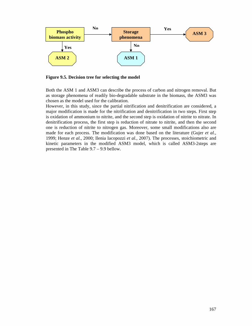
167

Figure 9.5. Decision tree for selecting the model

Both the ASM 1 and ASM3 can describe the process of carbon and nitrogen removal. But as storage phenomena of readily bio-degradable substrate in the biomass, the ASM3 was chosen as the model used for the calibration. However, in this study, since the partial nitrification and denitrification are considered, a major modification is made for the nitrification and denitrification in two steps. First step is oxidation of ammonium to nitrite, and the second step is oxidation of nitrite to nitrate. In denitrification process, the first step is reduction of nitrate to nitrite, and then the second one is reduction of nitrite to nitrogen gas. Moreover, some small modifications also are made for each process. The modification was done based on the literature (Gujer et al., 1999; Henze et al., 2000; Ilenia Iacopozzi et al., 2007). The processes, stoichiometric and kinetic parameters in the modified ASM3 model, which is called ASM3-2steps are presented in The Table 9.7 – 9.9 bellow.

Phospho biomass activity

ASM 3 Storage phenomena

No

ASM 2

Yes

ASM 1

No Yes

168

Table 9.7. Processes of ASM3_2steps

Processes Process rate

1 Hydrolysis

)3NO_H_X2NO_H_X(*

)3NO_H_X2NO_H_X/(S_XX_K

)3NO_H_X2NO_H_X/(S_X*h_k

+++

+

2 Aeration Storage Of COD

)3NO_H_X2NO_H_X(

*S_SS_K

S_S*

O_SO_K

O_S*STO_k

+++

3 Anoxic Storage Of COD

)3NO_H_X2NO_H_X(*S_SS_K

S_S*

3NO_S2NO_SNO_K

3NO_S2NO_S*

O_SO_K

O_K*NO_n*STO_k

++

+++

+

4 Aeration Respiration Of PHA STO_X*

O_SO_K

O_S*2O_STO_b

+

5 Anoxic Respiration Of PHA

STO_X*

3NO_S2NO_SNO_K

3NO_S2NO_S*

O_SO_K

O_K*NO_STO_b

+++

+

6 Aeration )O_SSat_O_S(*Actual_Kla −

7 Aeration Growth Of X_A_NH

NH_A_X*ALK_SHO_A_K

ALK_S*

NH_SNH_A_K

NH_S*

O_SNH_O_A_K

O_S*NH_A_

+

++µ

8 Aeration Growth Of X_A_NO2

2NO_A_X*ALK_SHO_A_K

ALK_S*

2NO_S2NO_A_K

2NO_S*

O_S2NO_O_A_K

O_S*2NO_A_

+

++µ

9 Aeration Endogenous

Respiration Of X_A_NH

NH_A_X*O_SNH_O_A_K

O_S*2O_A_b

+

10 Aeration Endogenous Respiration Of X_A_NO2

2NO_A_X*O_S2NO_O_A_K

O_S*2O_A_b

+

11 Anoxic Endogenous Respiration Of X_A_NH

NH_A_X*2NO_SNO_K

2NO_S*

O_SNH_O_A_K

NH_O_A_K*NO_A_b

++

12 Anoxic Endogenous Respiration Of X_A_NO2

2NO_A_X*3NO_SNO_K

3NO_S*

O_S2NO_O_A_K

2NO_O_A_K*NO_A_b

++

13 Aeration Growth Of X_H_NO2

2NO_H_X*2NO_H_X/STO_XSTO_K

2NO_H_X/STO_X*

ALK_SHO_K

ALK_S*

NH_SNH_K

NH_S*

O_SO_K

O_S*2NO_H_

+

+++µ

14 Aeration Growth Of X_H_NO3

3NO_H_X*3NO_H_X/STO_XSTO_K

3NO_H_X/STO_X*

ALK_SHO_K

ALK_S*

NH_SNH_K

NH_S*

O_SO_K

O_S*3NO_H_

+

+++µ

169

15 Anoxic Growth Of X_H_NO2

2NO_H_X*2NO_H_X/STO_XSTO_K

2NO_H_X/STO_X

*ALK_SHO_K

ALK_S*

NH_SNH_K

NH_S

*2NO_SNO_K

2NO_S*

O_SO_K

O_K*NO_n*2NO_H_

+

++

++µ

16 Anoxic Growth Of

X_H_NO3

3NO_H_X*3NO_H_X/STO_XSTO_K

3NO_H_X/STO_X

*ALK_SHO_K

ALK_S*

NH_SNH_K

NH_S

*3NO_SNO_K

3NO_S*

O_SO_K

O_K*NO_n*3NO_H_

+

++

++µ

17 Aeration Endogenous Respiration Of X_H_NO2

2NO_H_X*O_SO_K

O_S*2O_H_b

+

18 Aeration Endogenous Respiration Of X_H_NO3

3NO_H_X*O_SO_K

O_S*2O_H_b

+

19 Anoxic Endogenous Respiration Of X_H_NO2

2NO_H_X*2NO_SNO_K

2NO_S*

O_SO_K

O_K*NO_H_b

++

20 Anoxic Endogenous Respiration Of X_H_NO3

3NO_H_X*3NO_SNO_K

3NO_S*

O_SO_K

O_K*NO_H_b

++

170

Table 9.8a. Stoichiometrics parameters of ASM3_2steps 1

Process S_I S_S S_O S_NH S_N2 S_NO2 S_NO3

1 f_S_I 1 -

f_S_I )I_S_f1(*S_S_N_iS_X_N_i −−

2 - 1 2O_STO_Y1+− S_S_N_i

3 - 1 S_S_N_i

86.2

NO_STO_Y1−

72.1

)NO_STO_Y1( −− 86.2

)NO_STO_Y1( −−

4 - 1 5

86.2

1

6 1 7

NH_A_Y

43.31−

NH_A_Y

1BM_N_i −−

NH_A_Y

1

8

2NO_A_Y

14.11−

BM_N_i−

2NO_A_Y

1− 2NO_A_Y

1

9 )I_X_f1( −− I_X_N_i*I_X_fBM_N_i −

10 )I_X_f1( −− I_X_N_i*I_X_fBM_N_i −

11 I_X_N_i*I_X_fBM_N_i −

72.1

I_X_f1−

72.1

I_X_f1−−

12 I_X_N_i*I_X_fBM_N_i −

86.2

I_X_f1−

86.2

I_X_f1−−

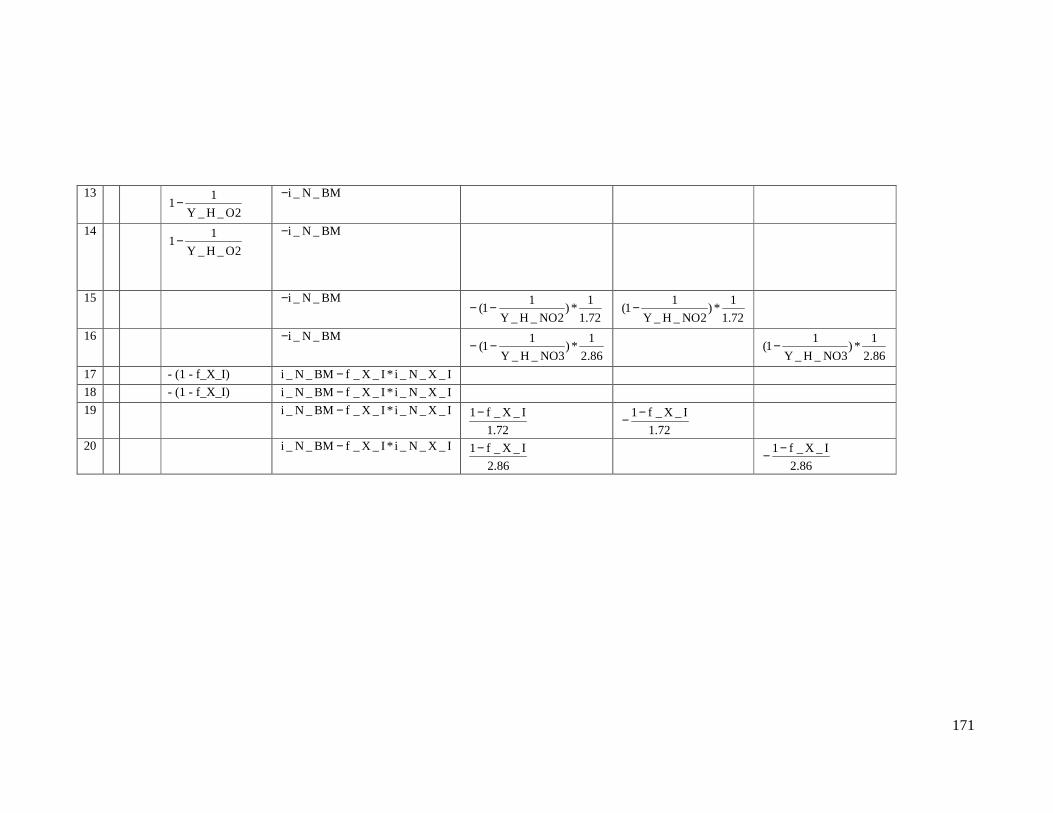
171

13

2O_H_Y

11−

BM_N_i−

14

2O_H_Y

11−

BM_N_i−

15 BM_N_i−

72.1

1*)

2NO_H_Y

11( −−

72.1

1*)

2NO_H_Y

11( −

16 BM_N_i−

86.2

1*)

3NO_H_Y

11( −−

86.2

1*)

3NO_H_Y

11( −

17 - (1 - f_X_I) I_X_N_i*I_X_fBM_N_i −

18 - (1 - f_X_I) I_X_N_i*I_X_fBM_N_i −

19 I_X_N_i*I_X_fBM_N_i −

72.1

I_X_f1−

72.1

I_X_f1−−

20 I_X_N_i*I_X_fBM_N_i −

86.2

I_X_f1−

86.2

I_X_f1−−

172

Table 9.8b. Stoichiometrics parameters of ASM3_2steps 2

Process S_ALK X_I X_S X_H_NO2 X_H_NO3 X_A_NH X_A_NO2 X_STO X_TSS

1

14

I_S_f1*S_S_N_iS_X_N_i

−− - 1 S_X_TS_i−

2

14

S_S_N_i

2O_STO_Y

2O_STO_Y*60.0

3

14

1*)

86.2

NO_STO_Y_1S_S_N_i( +

NO_STO_Y NO_STO_Y*60.0

4 - 1 -60 5

86.2*14

1

- 1 -60

6 7

14

1*)

NH_A_Y

2BM_N_i( −−

1 BM_TS_i

8

14

1*)

2NO_A_Y

2BM_N_i( −−

1 BM_TS_i

9

14

)I_X_N_i*I_X_fBM_N_i( −

2 - 1

BM_TS_i

I_X_TS_i*I_X_f

−

10

14

)I_X_N_i*I_X_fBM_N_i( −

2 - 1

BM_TS_i

I_X_TS_i*I_X_f

−

11

14

1*)

72.1

I_X_f1

I_X_N_i*I_X_fBM_N_i(

−+

−

f_X_I - 1

BM_TS_i

I_X_TS_i*I_X_f

−

12

14

1*)

86.2

I_X_f1

I_X_N_i*I_X_fBM_N_i(

−+

−

f_X_I - 1

BM_TS_i

I_X_TS_i*I_X_f

−

173

13

14

BM_N_i− 1

2O_H_Y

1− 2O_H_Y

60.0BM_TS_i −

14

14

BM_N_i− 1

2O_H_Y

1− 2O_H_Y

60.0BM_TS_i −

15

14

1*

)72.1

1*)

2NO_H_Y

11(BM_N_i( −+−

1

2NO_H_Y

1−

2NO_H_Y

60.0BM_TS_i −

16

14

1*

)86.2

1*)

3NO_H_Y

11(BM_N_i( −+−

1

3NO_H_Y

1−

3NO_H_Y

60.0BM_TS_i −

17

14

)I_X_N_i*I_X_fBM_N_i( −

f_X_I - 1

BM_TS_i

I_X_TS_i*I_X_f

−

18

14

)I_X_N_i*I_X_fBM_N_i( −

f_X_I - 1

BM_TS_i

I_X_TS_i*I_X_f

−

19

14

1*)

72.1

1I_X_f

I_X_N_i*I_X_fBM_N_i(

−−

−−

f_X_I - 1

BM_TS_i

I_X_TS_i*I_X_f

−

20

14

1*)

86.2

1I_X_f

I_X_N_i*I_X_fBM_N_i(

−−

−−

f_X_I - 1

BM_TS_i

I_X_TS_i*I_X_f

−

174

Table 9.9. Kinetics parameters of ASM3_2steps

k_h MaxSpecificHydrolysisRate Hydrolysis rate constant

b_A_NO DecayCoeffAutotr Anoxic endogenous respiration rate of X_A

b_A_O2 DecayCoeffAutotr Aerobic endogenous respiration rate of X_A

b_H_NO DecayCoeffHeterotr Anoxic endogenous respiration rate of X_H

b_H_O2 DecayCoeffHeterotr Aerobic endogenous respiration rate of X_H

b_STO_NO DecayCoeffHeterotr Anoxic respiration rate for X_STO b_STO_O2 DecayCoeffHeterotr Aerobic respiration rate for X_STO

F_BOD_COD Fraction Conversion factor BOD/COD f_S_I FractOfBiomassLeadingToPartProd Production of S_I in hydrolysis

f_X_I FractOfBiomassLeadingToPartProd Production of X_I in aerobic endogenous respiration

i_N_BM MassOfNitrogenPerMassOfCODInBiomass N content of biomass X_H, X_A i_N_S_I MassOfNitrogenPerMassOfCODInBiomass N content of S_I i_N_S_S MassOfNitrogenPerMassOfCODInBiomass N content of S_S

i_N_X_I MassOfNitrogenPerMassOfCODInBiomass N content of X_I i_N_X_S MassOfNitrogenPerMassOfCODInBiomass N content of X_S i_TS_BM FractOfBiomassLeadingToPartProd TSS to COD ratio for biomass X_H, X_A

i_TS_STO FractOfBiomassLeadingToPartProd TSS to COD ratio for X_STO based on PHB

i_TS_X_I FractOfBiomassLeadingToPartProd TSS to COD ratio for X_I i_TS_X_S FractOfBiomassLeadingToPartProd TSS to COD ratio for X_S K_A_HCO HalfSatCoeff Bicarbonate saturation for nitrifiers

K_A_NH HalfSatCoeff Ammonium substrate concentration for X_A_NH

K_A_NO2 HalfSatCoeff Ammonium substrate concentration for X_A_NO2

K_A_O_NH HalfSatCoeff Oxygen saturation for X_A_NH K_A_O_NO2 HalfSatCoeff Oxygen saturation for X_A_NO2 K_HCO HalfSatCoeff Bicarbonate saturation constant of X_H K_NH AmmonHalfSatCoeffForAutotr Ammonium saturation as nutrient K_NO NitrateHalfSatCoeffForDenitrifHetero Saturation constant for S_NO K_O OxygenHalfSatCoeffForHetero Saturation constant for S_O K_S HalfSatCoeffForHetero Saturation constant for substrate S_S k_STO MaxSpecifGrowthRateHetero Storage rate constant K_STO HalfSatCoeff Saturation constant for X_STO K_X HalfSatCoeffForHydrolSlowBioDegradeSubstr Hydrolysis saturation constant

mu_A_NH MaxSpecifGrowthRateAutotr Autotrophic max. growth rate of X_A_NH

mu_A_NO2 MaxSpecifGrowthRateAutotr Autotrophic max. growth rate of X_A_NO2

mu_H_NO2 MaxSpecifGrowthRateHetero Heterotrophic max. growth rate of X_H_NO2

mu_H_NO3 MaxSpecifGrowthRateHetero Heterotrophic max. growth rate of X_H_NO3

n_NO FractOfBiomassLeadingToPartProd Anoxic reduction factor S_O_Sat Concentration Oxygen saturation concentration Y_A YieldForAutotrophicBiomass Yield of autotrophic biomass per NO3_N Y_A_NH YieldForAutotrophicBiomass Yield of X_A_NH per NO3_N Y_A_NO2 YieldForAutotrophicBiomass Yield of X_A_NO2 per NO3_N

175

Y_H_NO YieldForHeterotrophicBiomass Anoxic yield of heterotrophic biomass per X_STO

Y_H_NO2 YieldForHeterotrophicBiomass Anoxic yield of X_H_NO2 per X_STO Y_H_NO3 YieldForHeterotrophicBiomass Anoxic yield of X_HNO3 per X_STO

Y_H_O2 YieldForHeterotrophicBiomass Aerobic yield of heterotrophic biomass per X_STO

Y_STO_NO YieldForHeterotrophicBiomass Anoxic yield of stored product per S_S Y_STO_O2 YieldForHeterotrophicBiomass Aerobic yield of stored product per S_S The effect of temperature on the kinetics was also considered in the model implementation using the Arrhenius equation (Henze et al., 2002). The default values of ASM3 and values from literatures were applied.

Step 6. Process characterization

6.a. Estimation of ASM parameters To make the calibration easier, it is important to determine experimentally some of the parameters of the activated sludge model. Therefore, some parameters can be fixed and the calibration goes through the remaining parameters. The literature shows that respirometry assays are commonly used for determining these parameters. In this study, two different assays were implemented. a1) Biotest to determine autotrophic max growth rate, yield, decay rate and ammonium substrate concentration of X_A_NH and X_A_NO2 (modified from) (Metcalf&Eddy, 1991). This work has already been presented in Chapter 7 (Item 7.2). The general results at 20.2oC and 24.98oC temperature are given in Table 9.10: Table 9.10. Kinetic and stoichiometric parameters of the studied activated sludge

Calibration (at 20.2 oC) Validation ( at 24.98 oC) Unit X_A_NH X_A_NO2 Overall X_A_NH X_A_NO2 Overall

Ks mgN/L 1.32 - 1.35 1.32 - 1.35 Y mgCOD/mgN 0.176 0.06 0.236 0.176 0.06 0.236

µm d-1 1.270 0.081 1.255 1.08 0.19 - bA d-1 0.03 0.03 - 0.054 0.054 -

a2) Oxygen uptake rate tests (for determination of heterotrophic yield (YH) The test was presented in Chapter 7 (item 7.3), the value of heterotrophic yield coefficient YH that was estimated is 0.683.

6.b. Determination of sludge concentration and biomass fractionation b1) SS and VSS determination SS (suspended solid) determined in the SBR at the beginning and at the end of calibration are 3.95 g/L and 11.3 g/L. Since VSS (volatile suspended solids) represent 77% and 60% of SS, relatively in each period, VSS are 3.0 g/L and 6.8 g/L, relatively. SS and VSS in discharged wastewater: Non settling part in the discharged wastewater (f_ns) at the end of cycle was determined through SS estimation. Average value of SS in

176

the steady state of the calibration period was very small, around 0.003 g/L together with the SS value in the SBR, yields an f_ns of 0.001. b2) Biomass composition Biomass composition analysis method was already presented in Chapter 5. Ratio of active biomass was done on sludge samples at the beginning and the end of calibration. As mentioned in Chapter VI, based on total of species of Nitrosomonas, Nitrosospira and Nitrobacter in the nature (Féray, 2000), total of ammonium and nitrite oxidizing bacteria was determined. Table 9.9 presents the results of amount of group of biomass according to MPN method. Denitrifying bacteria were calculated based on equations rates of denitrification (see Eq. 6.17 and 6.18 in Annex 6.2). As VSS in SBR at the beginning and the end of the calibration without carbon addition (calibration 1) was measured at 3.0 g/L and 6.8 g/L, respectively; at the end of validation 1 it was measured at 7.7 g/L. For calibration 2 at the beginning and the end it increased from 3.1 g/L to 9.12g/L, respectively. Concentrations of these bacteria were determined, which are presented in Table 9.11 and 9.12. SRT at the steady state of calibration 1 and validation 1 were kept around 45.7 d. Table 9.11. Amount of typical group of biomass measured by MPN method (MPN/ml)

Group of biomass Total VSS Nitrobacter Nitrosomonas Nitrosospira

(MPN/ml) (MPN/ml) (MPN/ml) (MPN/ml)

Begin of calibration 1 1.7*1010 4.5*108 3*108 3*108

End of calibration 1 5.4*109 4.1*107 0.44*109 1.85*107

End of validation 1 5.5*109 4.7*107 0.45*109 3.7*107

Begin of calibration 2 5.4*109 0.3*109 1.2*107 2.37*108

Table 9.12. Experimental biomass concentration in calibration and validation periods (gCOD/L)

Concentration (gCOD/L) X_A_NH X_A_NO2 X_H_NO2 X_H_NO3

Begin of calibration 1 0.23 0.19 0.36 0.44 End of calibration 1 1.20 0.13 - -

End of validation 1 1.38 0.13 - - Experime-tal data

Begin of calibration 2 0.37 0.34 0.58 0.59 Begin of calibration 1 0.23 0.19 0.36 0.44 End of calibration 1 1.19 0.13 0.35 0.38 Begin of validation 1 1.19 0.13 0.35 0.38

End of validation 1 1.39 0.11 0.43 0.36 Begin of calibration 2 0.37 0.34 0.58 0.59

End of calibration 2 1.39 0.54 9.20 0.36 Begin of validation 2 1.39 0.54 9.20 0.36

Simulated data (Begin for Input and End for output)

End of validation 2 1.37 1.21 8.60 1.07 Note: - calibration 1 and validation 1: without carbon addition - calibration 2 and validation 2: with carbon addition

177

It has been said that activated sludge subjected to nitrification and acclimation culture using a waste liquid in a sludge treatment such as dehydrated filtrate contains about 0.35% of nitrifying bacteria. When such an active sludge is used as a raw material and subjected to acclimation culture and accumulated for about two months in a liquid containing NH4 --N, amount of the nitrifying bacteria in the said activated sludge increases to an extent of about ten-fold (3.5%) (Patent, 2003). In this case, although ammonium oxidizing bacteria increased very well, the increase of nitrifying bacteria is about 3.34 times due to decrease of nitrite oxidizing bacteria.

6.c. Influent wastewater characterization The influent wastewater characterization was done based on the STOWA protocol with some modifications. This methodology is based on physical-chemical and BOD, COD and nitrogen measurements. Inlet leachate of the SBR pilot was sampled and analyzed intensively during the weeks of calibration. The buffer tank was fed with new leachate every week. The parameters include COD, COD after filtration with 0.45 µm filter paper, BOD, BOD after filtration with 0.45 µm filter paper, NH4

+. In the validation period, except BOD that was sampled only one time at the beginning of the period, the others parameters were sampled and analyzed four times per week. In the calibration period, the parameters were sampled and analyzed only at the beginning of the period. The results of nitrogen and COD evolution in influent of SBR were already presented in Graph 9.1 and Graph 9.2. It can be noted that, COD in inlet leachate did not changed very much, and COD is mostly inert COD, or slowly biodegradable COD. This is a typical characteristic of leachate in Vietnam. Ammonium decreased a little bit but not significantly, probably because the buffer tank has an open surface to the atmosphere and is thus more aerated than closed cans. Procedure for the influent wastewater fractionation The influent wastewater characterization was divided into the organic matter fractionation, the nitrogen fractionation and other substrate fractionation (in this case there are only oxygen and alkalinity). These were performed following the procedures described in Diagram 9.2, 9.3 and 9.4, which were based on the standard Dutch STOWA guidelines with some modifications.

178

Diagram 9.2. Characterization of Organic matter fractionation in the influent wastewater

Diagram 9.3. Characterization of Nitrogen fractionation in the influent wastewater

Diagram 9.4. Characterization of Oxygen and alkalinity fractionation in the influent wastewater

Table 9.13. Definition of organic matter and nitrogen compound.

Definition (compounds) Symbol Units Readily biodegradable organic S_S mg COD/L Inert soluble organic S_I mg COD/L Slowly biodegradable organic X_S mg COD/L Inert particulate organic X_I mg COD/L Total suspended solid X_TSS mg SS/L Ammonium S_NH mgN/L Nitrite S_NO2 mg COD/L Nitrate S_NO3 mg COD/L Nitrogen gas S_N2 mg COD/L

NH4+ NO2

- NO3-

S_NH S_NO2 S_NO3

N2

S_N2

O2 CaCO3

S_O S_AKL

COD inf_0.45

S_S + X_S + S_I + X_I

COD inf

BOD ultimate _0.45µm

S_S + S_I

S_S X_S S_I X_I X_STO X_A _NH

X_A _NO2

X_H _NO2

X_H _NO3

Ignored

X_TSS

BOD ultimate

S_S + X_S

179

BOD versus time_calibration

0

40

80

120

1 4 7 10 13 16 19 22 25 28 31 34 37 40

Time (day)

BO

D (

mg

O2/

L)

0.50

0.55

0.60

0.65

0.70

0.75

BOD_inf

BOD_inf_0.45

BOD_inf_0.45/BOD_inf

a) Determining the organic matters (S_S, S_I, X_S, X_I, X_TSS) COD of the influent leachate was analyzed and is equal to total COD: A = S_S + S_I + X_S + X_I (Eq. 9.2) The influent leachate was filtered with filter paper of 0.45µm, the filtrated solution then was analysed to get a COD which is equal to readily biodegradable organic (S_S) and inert soluble organic (S_I): B = S_S + S_I (Eq. 9.3) Ultimate (ATU) BOD of the influent leachate was observed, which is equal to readily biodegradable organic (S_S) and slowly biodegradable organic (X_S): C = S_S + X_S (Eq. 9.4) By the way, ultimate (ATU) BOD of the filtrated influent leachate was observed, which is equal to readily biodegradable organic (S_S): D = S_S (Eq. 9.5) Set of equations used for calculation of organic matters and nitrogen compounds. A = S_S + S_I + X_S + X_I (Eq. 9.2) B = S_S + S_I (Eq. 9.3) C = S_S + X_S (Eq. 9.4) D = S_S (Eq. 9.5) By solving the set of equations, we found values of S_I, X_S, and X_I. X_TSS is determined by method for SS estimation in the activated sludge system; with 1.2 µm filter. The value of this parameter therefore is smaller than that of total X_S and X_I because a part of it goes through the filter paper.

Graph 9.24. BOD test for influent leachate in calibration 1

Graph 9.25. BOD test for influent leachate in validation 1

b) Determining the biomass components All biomass components including nitrifying bacteria (X_A_NH, X_A_NO2), heterotrophic bacteria (X_H_NO2, X_H_NO3) as well as cell internal storage product of heterotrophic organisms (X_STO) were ignored, since total suspended solid (X_TSS) was considered only organic components (X_S and X_I). This assumption was based on the fact that ammonium concentration in the influent leachate did not changed very much. That means, there was almost no nitrification taking place in the buffer tank.

BOD versus time_calibration

0

20

40

60

80

100

120

1 4 7 10 13 16 19 22 25 28 31 34 37 40

Time (day)

BO

D (m

gO2

/L)

0.50

0.55

0.60

0.65

0.70

0.75

BOD_inf

BOD_inf_0.45

BOD_inf_0.45/BOD_inf

180

c) Determining the nitrogen compounds The S_NH, S_NO2 and S_NO3 are obtained from ammonium, nitrite and nitrate measurements. Results of the fractionation The average contribution of the organic components to the total COD, and the results of the influent ASM3_2step based on fractionation for organic matters and nitrogen are presented in Table 9.12. The results for the calibration as well as validation period are presented. Because COD concentration and ammonium as well in influent leachate in buffer tank did not change very much, concentration of these parameters used for calibration was taken as the average value for the whole period. Table 9.14. Characteristics of influent leachate and corresponding parameters for ASM3_2step in calibration and validation period with and without carbon addition in Vietnam and in Belgium

No carbon addition (Vietnam)

Carbon addition (Vietnam)

Carbon addition (Belgium)

Parameters Unit C V C V C V

Average Average Average Analysed parameters

CODinf mgO2/L 353 588 525 351 360 455

COD0.45µm mgO2/L 312 533 485 318 330 422

Ultimate BOD

mgO2/L 116 180 125 108 97 162

Ultimate BOD0.45µm

mgO2/L 80 130 90 78 76 149

N2-N mgN/L ignored ignored ignored ignored ignored ignored

NH4-N mgN/L 335 536 406 334 100 162

NO2-N mgN/L 0 53 48.0 0 6 0

NO3-N mgN/L 0 3 3.2 0 40 0

Alkalinity mgCaCO3/L 2570 3840 3740 2603 578 942

Oxygen mgO2/L 4.00 1.15 1.15 4.20 3.50 2

Biomass mgCOD/L ignored ignored ignored ignored ignored ignored ASM3_2step parameters

S_S mgCOD/L 80 130 90 78 76 149 X_S mgCOD/L 36 50 35 30 21 13 S_I mgCOD/L 233 403 395 240 254 273 X_I mgCOD/L 5 5 5 3 9 20

S_NH4 mgN/L 330 535 406 334 100 154

S_NO2 mgN/L 0.06 53 48.0 0 5.9 0.2

181

S_NO3 mgN/L 0.81 3 3.2 0 39.7 0.3

S_N2 mgN/L 0 0 0 0 0 0

X_A_NH mgCOD/L 0 0 0 0 0 0

X_A_NO2 mgCOD/L 0 0 0 0 0 0

X_H_NO2 mgCOD/L 0 0 0 0 0 0

X_H_NO3 mgCOD/L 0 0 0 0 0 0

X_STO mgCOD/L 0 0 0 0 0 0 X_TSS mgSS/L 36 50 37 30 28 30.7

Note: C - Calibration; V - Validation

9.3.4. STAGE IV: CALIBRATION AND VALIDATION

9.3.4.1. Nitrification and denitrification without external carbon addition

Step 7A. Calibration of the biokinetic model Calibration was implemented for a long term period, steady state and cycle evolution.

7A.a. Building SBR configuration. A configuration is a graphical model representation of the system. The experimental SBR1 is modeled by a configuration that is presented in Figure 9.6. Units in the configuration are described in Table 9.15.

Figure 9.6. Configuration of the experimental SBR1

15

I

CF

CF

CFC

F

Timer_1

Controler_1

O

OBT_1

SBR_1 CF_1

FC_1

FC_2

FC_3

Sensor_1 in_1

out_1

out_2

waste_1

182

Table 9.15. Description of configuration of the SBR1

Unit Description Function

BT_1 Buffer tank With a storm tank one tries to control the extra

amount of influent water. A storm tank is modeled as a tank with an effluent pump. The effluent has a variable flow rate that depends on the volume in the tank, the desired pump flow rate and the influent flow rate. The model flattens out the concentration peaks and also the flow rate peaks, within the limits. The content of the tank is supposed to be well mixed. In this case, it is used to store leachate.

SBR_1 SBR tank The model describes a sequencing batch reactor

process with two reaction phases (Nitrification (2 steps) and denitrification)

Timer_1 15

Timer 21 A timer gives a certain output according to the period.

Timer21 has two periods and has one controlling output per period. In this case, it controls the pumping time of the leachate from the buffer tank

Control_1 Controller This is a model for a proportional-integral-derivative

controller. The value of the manipulated variable changes proportionally to the value of the error signal, to the value of the integral and to the differential of the error function with time. This is done to solve the overshoot problem of a PI controller. It controls DO concentration (or Kla actual) in SBR tank from the signal of DO sensor.

Sensor_1 DO sensor Sensor measuring the dissolved oxygen concentration

in the SBR tank

CF_1 C

F

C_F Converter

This model is used to convert incoming data expressed in concentrations into fluxes (product of concentration and flow).

FC_1 C

F

F_C Converter

FC_2 C

F

F_C Converter

FC_3 C

F

F_C Converter

This model is used to convert fluxes (product of concentrations and flow) into concentrations and flow. FC_1 is for discharged wastewater. FC_3 is for discharged sludge. FC_2 is for by pass.

In_1I

Input Characteristic of inlet wastewater

Out_1 O

Output Characteristic of outlet wastewater

183

7A.b. Starting simulation process 7A.b.1. Volume and flow rate simulation Firstly, parameters concerning to the volume, flow rate must be calculated exactly to have an exact evolution of volume and flow rate (Q_in, Q_out, Q_waste etc.). Figure 9.7 presents the evolution of SBR volume during the calibration period and in the cycles.

Figure 9.7. Volume evolution of the SBR1 in the calibration period

7A.b.2. Nitrogen removal process simulation Firstly, a simulation and also an experiment of thirty days were performed to get a “nearly” steady state. At the end of this period, the cycle evolution was observed with a number of samples taken during the whole cycle. The values of parameters related to the dynamic behavior could be fitted. The kinetic and stoichiometric parameters (µA_NH, YA_NH, YA_NO2, YH_O2, bA, KA_NH), determined from biokinetic and respirometry tests were used as default values. However, some default values of kinetic and stoichiometric parameters available in ASM3 and literatures values for those added in the ASM3_2step were kept constant, while some others were adjusted step by step so that calculated state variables fit with observed ones. A procedure for the calibration of the biokinetic model was established, which combined BIOMATH (http://biomath.ugent.be) and STOWA (http://www.stowa.nl) procedures. This consisted in a step-wise methodology, which differentiated between the steady state calibration and the cycle (dynamic) evolution calibration. It was based on expert knowledge and consisted in five interaction steps that considered the sludge production, dynamics of DO, NH4

+, NO2- and NO3

-. The Diagram 9.5 shows the scheme of the methodology used for calibration, which is referred from literature (Tabares, 2006).

Time (day)

Vol

ume

of S

BR

( L

)

184

Diagram 9.5. Calibration procedure for Partial nitr ogen removal with two – step nitrification/denitrification without carbon additi on

1) Values of parameters found from measurements and biokinetic tests were applied, including f_ns, µA_NH, µA_NO2, YA_NH, YA_NO2, KA_NH, KA_NO2 and bA. 2) Values of f_S_I, f_X_I, i_N_S_I, i_N_X_I, i_N_X_S, i_N_BM, i_TS_X_S, i_TS_BM, i_TS_STO and F_BOD_COD were kept constant as default values of the model. Saturated oxygen is calculated depending on temperature following the Equation (HEMMIS, 2004): S_O_Sat = 14.65 – 0.41 * Temp + 0.00799 * Temp2 – 0.0000778 * Temp3 (Eq. 9.6) 3) Biomass production

Table 9.16. Concentration of biomass in calibration 1 (gCOD/L)

Concentration (gCOD/L) X_A_NH X_A_NO2 X_H_NO2 X_H_NO3 Begin of calibration 1 0.23 0.19 0.36 0.44 Experimental

data End of calibration 1 1.20 0.13 - - Begin of calibration 1 0.23 0.19 0.36 0.44 Simulated

data (Begin for Input and

End for output)

End of calibration 1 1.19 0.13 0.35 0.38

Simulated concentrations of ammonium and nitrite oxidizing bacteria at the beginning and at the end of the calibration period were compared to experimental values. Y_A_NH and Y_A_NO2 were finally adjusted to 0.159 and 0.083 to fit the two sets of values. Those values are closer to literature values than the ones issued from biokinetic tests.

Long term evolution

Nitrification OK?

Nitrite accumulation?

Denitrification OK

Calibration complete

DO OK?

No

µmANH, µmANO2, KNH, KNO2, KAONH,

KAONO2

Yes

Klaaer KNO, nNO. KSTO Klaanox, µmHNO2,

µmHNO3, YSTO

Yes

No

Yes Yes

Yes

Steady state evolution

Cycle evolution

COD present?

No denitrification

No

No

No

DO limiting?

Yes

No Biomass

production OK?

YA_NH, YA_NO2,

YH_NO2, YH_NO3

No

Yes

185

Figure 9.8. Simulated biomass evolution in calibration 1

As can be seen the biomass that is most changing during the test period is the ammonium oxidizing biomass (increasing), then nitrite oxidizing bacteria (decreasing). This is reasonable with a partial nitrification. The change of others biomasses is smaller during this period. 4) Nitrification profile : Parameters of DO controller was adjusted little by little to obtain a reasonable nitrification profile. Nitrification includes ammonium trends, nitrite trends, nitrate trends and DO trends. It is necessary to have a minimum Kla of 19.79 d-1 obtained in the first day of the steady state period so that ammonium was consumed completely, at least in the last day. However, this value will be further adjusted in the next steps. Figure 9.9 and 9.10 presents the nitrification profile and oxygen profile, which are obtained from the simulation process.

Figure 9.9. Simulated nitrification profile in calibration 1

In Figure 9.9, we can see that ammonium evolution is almost opposite with nitrite evolution since nitrate is not produced very much (~ 20-30 mgN/L) in comparison with nitrite production during the whole period. Because there is no carbon addition in this case, nitrite therefore is accumulated day by day following the increase of ammonium oxidation efficiency.

Time (day)

Time (day)

Bio

ma

ss in

SB

R (

g)

SB

R_N

utri

ent

s (m

g/L

)

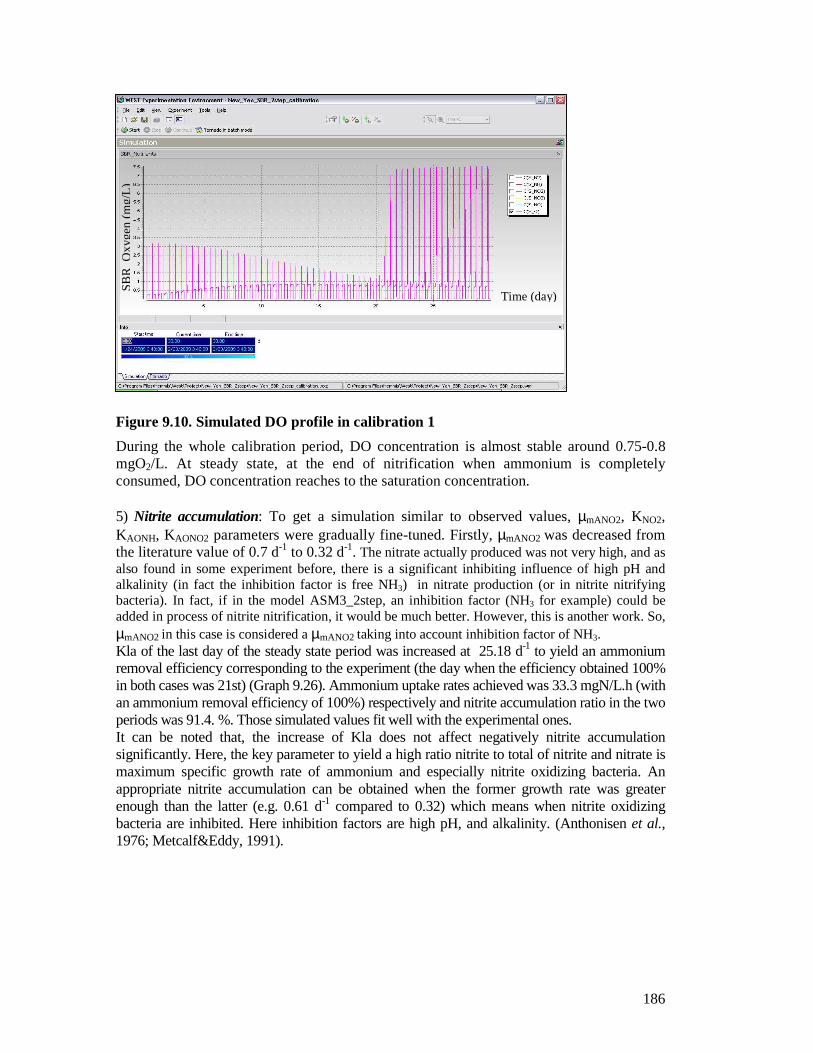
186

Figure 9.10. Simulated DO profile in calibration 1

During the whole calibration period, DO concentration is almost stable around 0.75-0.8 mgO2/L. At steady state, at the end of nitrification when ammonium is completely consumed, DO concentration reaches to the saturation concentration. 5) Nitrite accumulation: To get a simulation similar to observed values, µmANO2, KNO2, KAONH, KAONO2 parameters were gradually fine-tuned. Firstly, µmANO2 was decreased from the literature value of 0.7 d-1 to 0.32 d-1. The nitrate actually produced was not very high, and as also found in some experiment before, there is a significant inhibiting influence of high pH and alkalinity (in fact the inhibition factor is free NH3) in nitrate production (or in nitrite nitrifying bacteria). In fact, if in the model ASM3_2step, an inhibition factor (NH3 for example) could be added in process of nitrite nitrification, it would be much better. However, this is another work. So, µmANO2 in this case is considered a µmANO2 taking into account inhibition factor of NH3. Kla of the last day of the steady state period was increased at 25.18 d-1 to yield an ammonium removal efficiency corresponding to the experiment (the day when the efficiency obtained 100% in both cases was 21st) (Graph 9.26). Ammonium uptake rates achieved was 33.3 mgN/L.h (with an ammonium removal efficiency of 100%) respectively and nitrite accumulation ratio in the two periods was 91.4. %. Those simulated values fit well with the experimental ones. It can be noted that, the increase of Kla does not affect negatively nitrite accumulation significantly. Here, the key parameter to yield a high ratio nitrite to total of nitrite and nitrate is maximum specific growth rate of ammonium and especially nitrite oxidizing bacteria. An appropriate nitrite accumulation can be obtained when the former growth rate was greater enough than the latter (e.g. 0.61 d-1 compared to 0.32) which means when nitrite oxidizing bacteria are inhibited. Here inhibition factors are high pH, and alkalinity. (Anthonisen et al., 1976; Metcalf&Eddy, 1991).

Time (day)

SB

R_O

xyge

n (m

g/L

)

187

Simulated vs Experimental value of nitrogen compoun ds in outlet in calibration period

-50

0

50

100

150

200

250

300

350

0 5 10 15 20 25 30

Time (day)

Nitr

ogen

(m

gN/L

)

Simulated NH4

Simulated NO2

Simulated NO3

ExperimentalNH4ExperimentalNO2

ExperimentalNO3

Simulated vs experimental value of nitrogen compoun ds in the cycle evolutionCycle 31th (day 16th) and Cycle 41st (day 21th) and cycle 55th (day 28th)

0

50

100

150

200

250

300

350

0 2 4 6 8 10 12 2 4 6 8 10 12 2 4 6 8 10 12

Time (h)

Nitr

ogen

(mgN

/L)

SimulatedNH4SimulatedNO2

SimulatedNO3ExperimentalNH4ExperimentalNO2

ExperimentalNO3

Settling +Decan + Idle

Filling + React aeration

React anoxic

Settling +Decan + Idle

Filling + React aeration

React anoxic

Settling +Decan + Idle

Filling + React aeration

React anoxic

Graph 9.26. Simulated versus experimental nitrogen profile in outlet in calibration 1

Cycle calibration: µmANO2 had to be decreased to 0.108 d-1 to decrease nitrate that is produced at the end of nitrification process. KAO_NH and KAO_NO2 were fine-tuned from literature values of 0.5 and 1 mg O2 /L to 1.37 and 1.59 mg O2/L, respectively to better take into account the limiting effect of oxygen, (Graph 9.27 and 9.28). This can be explained that, due to the difficult penetration of oxygen into the bioflocs, a high concentration of oxygen in the system does not express the concentration of oxygen inside bioflocs. The influence of high concentration of nitrite and nitrate can be significant. This could also be due to a non optimal location-calibration of the DO sensor.

Graph 9.27. Simulated versus experimental Nitrogen profile in cycles 31, 41 & 55 (calibration 1)

188

Simulation vs. experimental value of DO in cycleCycle 31st, 41st, 43th and 55th (day 16th, 21st, 2 2nd and 28th)

-1

0

1

2

3

4

5

6

7

8

0 4 8 12 4 8 12 4 8 12 4 8 12

Time (h)

DO

(m

g/L)

-1

0

1

2

3

4

5

6

7

816

.016

.116

.2

16.3

16.4

16.5

21.1

21.2

21.3

21.4

21.5

22.1

22.2

22.3

22.4

22.5

28.1

28.2

28.3

28.4

28.5

ExperimentalDO

SimulatedDO

Graph 9.28. Simulated versus experimental DO profile in cycles 31, 41, 43 & 55 (calibration 1)

5) Denitrification: When the nitrification profile and nitrite accumulation were correctly simulated the calibration was tuned for denitrification. As the system is not closed completely and observed DO are not exactly zero but close to 0.05 – 0.1 mg/L, a Klaanox of 0.1 h-1was adopted. Nitrite and nitrate denitrification rate depend on µHNO2, µHNO3, n_NO, K_NO. The most important substrate in denitrification is biodegradable COD which is very low in old leachate, and moreover has partially been degraded in the preceding nitrification process, or even stored partly in the biomass cells (in the form of X_STO), then was liberated and combined with COD produced from biomass decay. The denitrification in this case therefore could be called endogenous denitrification. This COD participates into denitrification. The denitrification rate therefore also depends on k_STO, Y_STO_NO and Y_STO_O2. Y_STO_O2 was increased from literature values of 0.85 to 0.87 to increase storage capability of COD in the biomass cells in the aeration phase, saving more COD for the denitrification process; then Y_STO_NO was decreased from 0.8 to 0.63 to reduce storage capability of COD in biomass cells during the anoxic phase. However these values should be verified in the calibration with carbon addition since its effect would be clearer. Varying of µHNO2 and µHNO3 does not change very much the nitrite and nitrate removal efficiency. These values therefore were kept constant and could be adjusted in a further step when simulating biomass production. At the same time, adjustment of K_NO and K_STO did not change denitrification efficiency significantly. It is found that, in the experiment, nitrite and nitrate denitrification efficiency with biodegradable COD in the influent leachate was low. Then, n_NO (0.6) was increased to a higher value (0.7) and k_STO was adjusted from default value of the model of 5 to 3.2 to make nitrite and nitrate denitrification efficiency similar with the experiment. However, the changing of the parameters regarding to this denitrification process does not bring a notable change in the efficiency.

189

Step 8A. Validation without carbon addition The validation process consists in using the calibrated model with a set of data that is different from the calibration set. In this period, a ten day simulation was run applying some operating changes and taking into account the influent variability. The composition of influent was presented above. Instead of the 7 liter - maximum working volume, the 6 liter - one was applied in this period with higher oxygen supply intensity. Kla value of the filling-aerated as well as in aerated react phases therefore was changed. Kla value obtained in the filling-aerated phase is 28.5 h-1 that was presented in Figure 9.2. The Kla value obtained at the first day of the steady state in this simulation is also 28.5 h-1. Normally, there was no change in the kinetic and stoichiometric parameters. But temperature in this period was increased significantly (from 20.2 to 24.98oC) so the parameters most affected by temperature, including maximum specific growth rate (µA), decay constant (bA), oxygen saturation coefficient KAO of ammonium and nitrite oxidizing bacteria were increased according to the given temperature, µA_NH from 0.61 to 0.987 d-1, µA_NO2 from 0.108 to 0.17 d-1, bA from 0.03 to 0.049 d-1 and KA_O_NH and KA_O_NO2 from 1.37 and 1.59 to 1.76 and 1.97 mgO2/L, respectively. With a higher temperature, DO in the system is decreased. Ammonium uptake rates achieved during validation periods was 56.7 mgN/L.h (with an ammonium removal efficiency of 100%) respectively and nitrite accumulation ratio in the two periods was 95.6 %, respectively. Those simulated values fit well with the experimental ones.

Table 9.17. Concentration of biomass in validation 1

Concentration (gCOD/L) X_A_NH X_A_NO2 X_H_NO2 X_H_NO3 Begin of validation 1 1.20 0.13 - - Experimental

data End of validation 1 1.38 0.13 - -

Begin of validation 1 1.19 0.13 0.35 0.38 Simulated data (Begin for Input and End for output)

End of validation 1 1.39 0.11 0.43 0.36

Figure 9.11. Simulated biomass evolution during validation 1

Time (day)

SB

R_N

Biom

ass

(g)

190

Simulated vs Experimental value of nitrogen compoun ds in outlet in validation period

-100

0

100

200

300

400

500

600

1 3 5 7 9

Time (day)

Nitr

ogen

(m

gN/L

)

Simulated NH4

Simulated NO2

Simulated NO3

ExperimentalNH4ExperimentalNO2

ExperimentalNO3

8A.a. Validation at steady state Figure 9.12 presents Nitrification profile (including ammonium, nitrite, nitrate and oxygen trends) obtained from the validation period. Figure 9.13 presents DO profile in the validation period. Graph 9.29 presents simulated and experimental Nitrogen profile in the validation period.

Figure 9.12. Simulated nitrification profile in validation 1

Figure 9.13. Simulated oxygen profile in validation 1

Graph 9.29. Simulated versus experimental Nitrogen profile in outlet in validation 1

8A.b. Validation in cycle Graphs 9.30 and 9.31 present results obtained from cycle measurements (9th day) in the validation period, showing a good fit between the simulated and experimental values for the nitrogen and oxygen compounds.

Time (day) Time (day)

SB

R_N

utri

ent

s (m

g/L

)

SB

R_O

xyge

n (m

g/L

)

191

Simulated vs experimental value of nitrogen compoun ds in the cycle evolution in validation period

Cycle 17th (day 9th) and cycle 19th (day 10th)

0

100

200

300

400

500

600

0 2 4 6 8 10 12 2 4 6 8 10 12Time (h)

Nitr

ogen

(mgN

/L)

SimulatedNH4SimulatedNO2

SimulatedNO3ExperimentalNH4ExperimentalNO2

ExperimentalNO3

Filling + React aeration

React anoxic

Settling + Decan + Idle

Filling + React aeration

React anoxic

Settling +Decan + Idle

Simulation vs. experimental value of DO in cycleCycle 17th (day 9th)

-1

0

1

2

3

4

5

6

7

8

0 1 2 3 4 5 6 7 8 9 10 11 12

Time (h)

DO

(m

g/L)

-1

0

1

2

3

4

5

6

7

88.

08.

08.

18.

18.

28.

28.

28.

38.

38.

48.

48.

48.

5

ExperimentalDO

SimulatedDO

Graph 9.30. Simulated versus experimental Nitrogen profile in cycles 17 and 19 (validation)

Graph 9.31. Simulated versus experimental Oxygen profile in the cycle 17 (validation)

192

RESULTS OF CALIBRATION AND VALIDATION IN CASE OF NO CARBON ADDITION (FOR 8A) In Table 9.18, kinetic, stoichiometric and Kla values obtained during calibration and validation are presented. * Values varied with temperature Table 9.18. Kinetic, stoichiometric and Kla values of calibration and validation period

This study – ASM3_2step Parameters Unit

Default ASM3 Model

Literature (Henze et al.,

1999; Henze et al., 2002) (20oC)

Calibration (20.2oC)

Validation (25.98oC)*

b_A_O2 d-1 0.15 0.03 0.03 0.049* K_A_NH mgN/L 0.5 1.32 1.32 K_A_NO2 mgN/L 1 1 1 K_A_O_NH mgCOD/L 0.75 1.37 1.76 K_A_O_NO2 mgCOD/L 1 1.59 1.97 k_h mgCOD/(mgCOD*d) 3 K_HCO mgCOD/L 0.1 K_NO mgNO3-N/L 0.5 K_O mgCOD/L 0.2 K_S mgCOD/L 2 k_STO d-1 5 3.2 3.2 K_STO mgCOD/L 1 K_X mgCOD/mgCOD 1 µ_A_NH d-1 0.6 0.61 0.987* µ_A_NO2 d-1 0.7 0.108 0.17* µ_H_NO2 d-1 4.5 µ_H_NO3 d-1 4.5 n_NO - 0.6 0.7 0.7 S_O_Sat mgO2/L 8 8 8 Y_A_NH mgCOD/mgN 0.1562 0.159 0.159 Y_A_NO2 mgCOD/mgN 0.085 0.083 0.083 Y_H_NO mgCOD/mgCOD 0.54 Y_H_NO2 mgCOD/mgCOD 1 Y_H_NO3 mgCOD/mgCOD 1 Y_H_O2 mgCOD/mgCOD 0.63 0.67 0.67 Y_STO_NO mgCOD/mgCOD 0.8 0.63 0.63 Y_STO_O2 mgCOD/mgCOD 0.85 0.87 0.87 Kla react 1 end

h-1 - - 25.18 33.1*

193

CONCLUSION IN CASE OF NO CARBON ADDITION (FOR 8A) Based on an appropriate model base, simulation and modeling of the partial nitrification and denitrification in the activated sludge - SBR treating leachate was successful. However, the temperature change during the experimental period hampered the calibration and even more the validation of model parameters. Using biokinetic tests to determine some kinetic and stoichiometric parameters, especially specific growth rates could fater the calibration process. The simulation of nitrogen profiles according to the experiment is successful, particularly the nitrite profile. The activated sludge used for the study expressed its high nitrification capability with the presence of nitrifying bacteria, mostly increase of the ammonium oxidizing bacteria. The studied leachate is characterized by high pH and alkalinity, causing inhibition of nitrite oxidizing bacteria. Dissolved oxygen just showed its influence (negatively) in nitrite accumulation at the end nitrification at steady state, when ammonium is completely consumed and alkalinity remains low. This caused a decrease in pH, activating the nitrite oxidizing bacteria strongly again. However, time of this period is not long, thus total nitrite accumulation remains very high, of 91.4 and 95.6% in the calibration and validation period, respectively. Optimization of the partial nitrification and improvement of nitrogen removal efficiency will be continued in a next study, by adjusting DO, HRT (working volume of SBR) and cycles (time for each phase). The developed model will be used to optimize the process, and the optimized system will be checked by new experiments.

9.3.4.2. Nitrification and denitrification with external carbon addition

Step 7B. Calibration of the biokinetic model Calibration was implemented for long term period, a “nearly steady state” period and a cycle evolution.

7B.a. Building SBR configuration. The experimental SBR is modeled by a configuration that is presented in Figure 9.14. Because a unit SBR in the available model base only support for carbon addition in the first period of a timer (in this case it is Timer_2), so to overcome this inconvenience, a unit CFID (PointSettler2PhaseReact) is being used to replace the SBR. This model describes a continuous flow with intermittent decant batch process with two reaction phases. This process is also known as the IDEA process (Intermittently Decanted Extended Aeration). Units in the configuration are described in Table 9.19.

194

Figure 9.14. Configuration of the experimental SBR2

Table 9.19. Description of configuration of the SBR

Unit Description Function

BT_1

Buffer tank The same as in Table 9.15

SBR_1*

SBR tank (CFID PointSettler2PhaseReact)

The modified model describes a continuous flow with intermittent decant batch process with three reaction phases (nitrification in aeration phase and denitrification in anoxic phase (including settling phase). This in fact works like a sequencing batch reactor.

Timer_1 15

Timer 21 The same as in Table 9.15

Timer_2 15

Timer 31 Timer31 has three periods and has one controlling output per period. It controls pumping time of carbon source (with a constant flow rate) from the Dosing_unit

Control_1

Controller The same as in Table 9.15

Sensor_1

DO sensor The same as in Table 9.15

Dosing_unit_1

R S41 26-39

Dosing unit The Acetate model describes the in-line addition of acetate (CH3COOH) as an external carbon source. It is used to supply carbon source (e.g. acetate) to the SBR tank.

Interface link The one between the Dosing unit and the SBR is to control concentration of carbon source from the Dosing unit in accordance with total of nitrite and

15

I

CF

CFC

F

Timer_1

Controler_1

O

BT_1

SBR_1*

CF_1 FC_1

FC_3

Sensor_1 in_1

out_1

waste_1

15

R S41 26-39

Timer_2

Dosing_unit_1

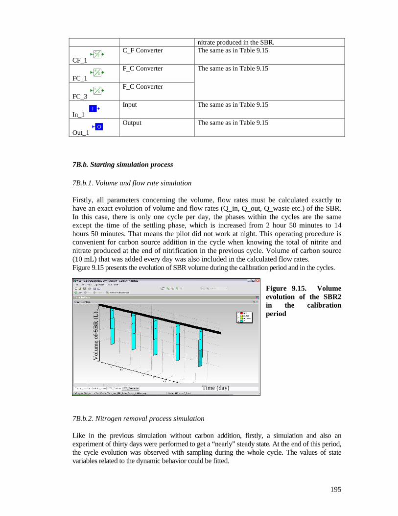
195

nitrate produced in the SBR.

CF_1 C

F

C_F Converter The same as in Table 9.15

FC_1 C

F

F_C Converter

FC_3 C

F

F_C Converter

The same as in Table 9.15

In_1I

Input The same as in Table 9.15

Out_1 O

Output The same as in Table 9.15

7B.b. Starting simulation process 7B.b.1. Volume and flow rate simulation Firstly, all parameters concerning the volume, flow rates must be calculated exactly to have an exact evolution of volume and flow rates (Q_in, Q_out, Q_waste etc.) of the SBR. In this case, there is only one cycle per day, the phases within the cycles are the same except the time of the settling phase, which is increased from 2 hour 50 minutes to 14 hours 50 minutes. That means the pilot did not work at night. This operating procedure is convenient for carbon source addition in the cycle when knowing the total of nitrite and nitrate produced at the end of nitrification in the previous cycle. Volume of carbon source (10 mL) that was added every day was also included in the calculated flow rates. Figure 9.15 presents the evolution of SBR volume during the calibration period and in the cycles.

Figure 9.15. Volume evolution of the SBR2 in the calibration period

7B.b.2. Nitrogen removal process simulation Like in the previous simulation without carbon addition, firstly, a simulation and also an experiment of thirty days were performed to get a “nearly” steady state. At the end of this period, the cycle evolution was observed with sampling during the whole cycle. The values of state variables related to the dynamic behavior could be fitted.

Time (day)

Vol

ume

of

SB

R (

L)

196

Because the calibration was implemented after the validation of case A (simulation without carbon addition), temperature in this period increased to 26.9o C (average value). Sludge was used for this calibration came from the same source than the one used for the previous calibration, therefore the kinetic and stoichiometric parameters (µA_NH, YA_NH, YA_NO2, YH_O2, bA, KA_NH), determined from biokinetic and respirometry tests were used as default values. A similar procedure for the calibration of the biokinetic model was established, which combined BIOMATH (http://biomath.ugent.be) and STOWA (http://www.stowa.nl) procedures. The Diagram 9.6 shows the scheme of the methodology used for calibration. Diagram 9.6. Calibration procedure for Partial nitr ogen removal with two – step nitrification/denitrification with carbon addition

1) Values of parameters found from measurements and biokinetic tests were applied, including f_ns (0.001), µA_NH (1.2 d-1), bA (0.054 d-1), KA_NH, KA_NO2 at the present temperature (26.9oC). 2) YA_NH, YA_NO2, results of the last calibration were used for this calibration. There is no calibration for biomass in this case. However, the results of simulation process are shown in Figure 9.16.

Long term evolution

Nitrification OK?

Nitrite accumulation?

Denitrification OK

Calibration complete

DO OK?

No

µmANH, µmANO2, KNH, KNO2, KAONH,

KAONO2

Yes

Klaaer KNO, nNO. KSTO Klaanox, µmHNO2,

µmHNO3, YSTO

Yes

No

Yes Yes

Yes

Steady state evolution

Cycle evolution

COD OK?

Redundancy/Deficiency

of COD

No

No

No

DO limiting?

Yes

No Biomass

production OK?

YA_NH, YA_NO2,

YH_NO2, YH_NO3

No

Yes

SND No Supplement

of COD

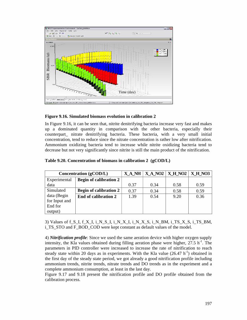
197

Figure 9.16. Simulated biomass evolution in calibration 2

In Figure 9.16, it can be seen that, nitrite denitrifying bacteria increase very fast and makes up a dominated quantity in comparison with the other bacteria, especially their counterpart_ nitrate denitrifying bacteria. These bacteria, with a very small initial concentration, tend to reduce since the nitrate concentration is rather low after nitrification. Ammonium oxidizing bacteria tend to increase while nitrite oxidizing bacteria tend to decrease but not very significantly since nitrite is still the main product of the nitrification. Table 9.20. Concentration of biomass in calibration 2 (gCOD/L)

Concentration (gCOD/L) X_A_NH X_A_NO2 X_H_NO2 X_H_NO3

Experimental data

Begin of calibration 2 0.37 0.34 0.58 0.59

Begin of calibration 2 0.37 0.34 0.58 0.59 Simulated data (Begin for Input and End for output)

End of calibration 2 1.39 0.54 9.20 0.36

3) Values of f_S_I, f_X_I, i_N_S_I, i_N_X_I, i_N_X_S, i_N_BM, i_TS_X_S, i_TS_BM, i_TS_STO and F_BOD_COD were kept constant as default values of the model. 4) Nitrification profile : Since we used the same aeration device with higher oxygen supply intensity, the Kla values obtained during filling aeration phase were higher, 27.5 h-1. The parameters in PID controller were increased to increase the rate of nitrification to reach steady state within 20 days as in experiments. With the Kla value (26.47 h-1) obtained in the first day of the steady state period, we got already a good nitrification profile including ammonium trends, nitrite trends, nitrate trends and DO trends as in the experiment and a complete ammonium consumption, at least in the last day. Figure 9.17 and 9.18 present the nitrification profile and DO profile obtained from the calibration process.

SB

R_

Bio

ma

ss (

g)

Time (day)

198

Figure 9.17. Simulated Nitrification profiles in calibration 2

Figure 9.18. Simulated DO profiles in calibration2

5) Nitrite accumulation: With the values of the kinetic and stoichiometric parameters found in the last calibration, nitrite accumulation was already obtained. However, in the last days of calibration, simulated nitrate was produced at a much higher value than what we got from the experiments. Changing of Y_STO_NO (anoxic yield stored product per S_S) from the value (0.63) of the last calibration to 0.82 brought about a better simulated profile for NO3. This means, when S_S is more stored for the next cycle, there will be more carbon available during nitrification process, increasing SND, and then reducing nitrate produced.

Time (day)

Time (day)

SB

R_N

utri

ent

s (m

g/L

) S

BR

_Oxy

gen

(mg/

L)

199

Simulated vs. Experimental Nitrogen profile at the beginning of cycle

-50

0

50

100

150

200

250

300

350

400

0.25

2.254.25 6.2

58.25

10.2512.25

14.25

15.2518.25

20.25

Time (day)

Nitr

ogen

(mgN

/L) Sim-NH4

Sim-NO2

Sim-NO3

Exp-NH4

Exp-NO2

Exp-NO3

Simulated vs. Experimental Nitrogen profile at the end of Nitrification

0

50

100

150

200

250

300

350

1 3 5 7 9 11 13 15 17 19 21

Time (day)

Nitr

ogen

(m

gN/L

) Sim-NH4

Sim-NO2

Sim-NO3

Exp-Nh4

Exp-NO2

Exp-NO3

This also has a meaning in saving some COD for the settling process when denitrification still occurs. µmANH was increased according to the given temperature to 1.2 d-1, while µmANO2 was decreased from 0.17d-1 of the last validation to 0.13 d-1 to have a good nitrite accumulation and also a good profile of nitrate not far different from the experiments. At the same time, an ammonium removal efficiency corresponding to the experiment (the day when the efficiency obtained 100 % was around day 16th) was achieved (Graph 9.32 and 9.33).

Graph 9.32. Simulated versus experimental Nitrogen profile at the beginning of cycle (calibration 2)

Graph 9.33. Simulated versus experimental Nitrogen profile at the end of Nitrification (calibration 2)

5) Denitrification: When the nitrification profile and nitrite accumulation were correctly simulated the calibration was tuned for denitrification. In this case, although observed DO was almost zero due the presence of a biodegradable carbon source, a Klaanox of 0.1 h-1was still adopted. Almost all the parameters defined in the last calibration without carbon were kept in this calibration and denitrification was already correctly simulated with the experiment. In the experiment, a source of carbon (in our case sugar, which is transformed into an equivalent COD acetate is used in the model) was added during denitrification of the present cycle based on the concentration of nitrite and nitrate produced in the previous one. However, a calculation that would not be very precise would induce an extra amount of COD at the end of denitrification, even this COD will be used during the settling phase when nitrate and nitrite are not completely reduced at the end of the anoxic phase. Moreover, storage phenomenon of substrate in the biomass, in this case known as Y_STO_NO and Y_STO_O2 also cause an amount of available readily degradable carbon during the next nitrification. Simultaneous nitrification and denitrification (known as SND) phenomenon was observed in almost aeration phase (when nitrification process is expected to be the main process ). The average ratio of SND (total of nitrite and nitrate produced / total ammonium consumed) in the aeration phase was around 0.675. Therefore, in the simulation model, an amount of carbon source (expressed thought M_acetate which is calculated based on the concentration C_Dose and flowrate Q_Dose) has to be calculated so that we also get an SND with a similar ratio as in the experiments. The average ratio of SND found is 0.646. M_acetate in the model is converted to Out_flow C(S_S) that will be In_flow C(S_S) of the SBR and is the main source of readily biodegradable COD for denitrification in the anoxic phase and also in the settling phase. Contrary to the constant Q_Dose, C_Dose is controlled by concentration of total NO2

- and

200

NO3- that are produced in the SBR at the end of nitrification process. This value therefore

is changed from cycle to cycle. The relationship between C_Dose in the Dosing_unit and (C_NO2

- + C_NO3-) in the SBR

found for this Q_Dose (10 mL/day) is: C_Dose = (1.71* C_NO2

- + 2.86 * C_NO3-) * 654. (Eq. 9.7)

Where 654 is the dilution factor from the concentrated acetate solution. However, it is also required an amount of organic matter used for biosynthesis which is more or less double than that used for energy production (see more in 2.1.2.3). By the way, because rate of denitrification depends very much on concentration of readily biodegradable COD, therefore to fit the simulation results with the experimental one, especially taking into account the concentration at the end of nitrification process, it is necessary to multiply “2.3” the amount of theoretically added carbon source. The Equation 9.7 now becomes: C_Dose = (1.71* C_NO2

- + 2.86 * C_NO3-) * 654 * 2.3 (Eq. 9.8)

Evolution of parameters (M_Acetate (a), Ouflow C(S_S) (b), C_Dose (c) of Dosing_unit and C(S_S) in the SBR (d) in SBR are presented on Figure 9.19.

Figure 9.19. Simulated external carbon profile in calibration2

c

a

b

d

Time (day) Time (day)

Time (day)

Ace

tate

_do

se (

mg/

L)

Out

flow

_C(S

_S)

(mg/

L)

SB

R_

C(S

_S)

(mg/

L)

201

Simulated vs. Experimental added C(S_S) in calibrat ion with carbon addition

0

200

400

600

800

1000

1200

1400

1600

1.26

3.26

5.26

7.26

9.26

11.26

13.26

15.26

17.26

19.26

Time (day)

C(S

_S) (

mg

O2/

L)

Sim-addedC(S_S)Exp-added

Simulated vs. Experimental Nitrogen proflile at the end of Cycle

-0.1

0.9

1.9

2.9

3.9

4.9

1 3 5 7 9 11 13 15 17 19

Time (day)

Nitr

oge

n (m

N/L

)

Sim-NO2

Sim-NO3

Exp-NO2

Exp-NO3

Simulated vs. Experimental Nitrogen profile at the end of Denitrification

-50

0

50

100

150

200

250

300

350

0.34 5.34 10.34 15.34 20.34

Time (day)

Nitr

og

en (

mgN

/L) Sim-NH4

Sim-NO2

Sim-NO3

Exp-NH4

Exp-NO2

Exp-NO3

Then, n_NO (0.7) in the last calibration was increased to the maximum value (1) and k_STO was adjusted from the last value 3.2 to 3.0 to increase the denitrification efficiency and fit with the experiment.

Graph 9.34. Simulated versus experimental carbon (C(S_S)) profile in calibration 2

Graph 9.35. Simulated versus experimental Nitrogen profile at the end of denitrification (calibration 2)

Graph 9.36. Simulated versus experimental Nitrogen profile at the end of cycle (calibration 2)

Cycle calibration: KAONH, KAONO2 were fine-tuned from the values of the last validation from 1.76 and 1.97 to 1.11 and 1.43 mgO2/L, respectively, to get DO profile that is nearly similar to the records. These values of KAO in this calibration were smaller than that in the last calibration and validation even if temperature is higher in this period. Since nitrate and nitrite were completely consumed at the end of a cycle, there is no increased accumulation of nitrate and nitrite at the beginning of the next cycles. The absence of nitrite and nitrate in the environment could well facilitate the penetration of oxygen into the bioflocs (Graph 9.37 and 9.38).

202

Simulated vs. Experimental Nitrogen profile in cycl eCycle 40th (day 20th)

0

50

100

150

200

250

300

350

20 20

20.1

20.1

20.2

20.2

20.2

20.3

20.3

20.4

20.4

20.4

20.5

Time (hour)

Nitr

ogen

(m

gN/L

)

Sim-NH4

Sim-NO2

Sim-NO3

Exp-NH4

Exp-NO2

Exp-NO3

Nitrification Denitr Settling

Simulated vs. Experimental DO profile in cycle Cycl e 24th, 34th and 40th (day 12th, 17th and 20th)

-10123456789

12.0

12.1

12.2

12.3

12.4

17.0

17.1

17.3

17.4

17.5

20.1

20.2

20.3

20.4

Time (hour)

DO

(m

gO

2/L)

0.00

3.00

6.00

9.00

12.00

2.99

5.99

8.99

11.99

2.98

5.98

8.98

11.98

Sim-DO

Exp-DO

Time (day)

Graph 9.37. Simulated versus experimental Nitrogen profile in the cycle 40th (calibration 2)

Graph 9.38. Simulated versus experimental DO profile in the cycle 24, 34 and 40th (calibration 2)

Step 8B. Validation with carbon addition The validation process consists in using the calibrated model with a different set of data. In this period, a twenty day simulation was run applying the influent variability. In this case, the daily composition of influent changed much more than that in the validation without carbon addition presented above. The other parameters in the operating procedure (volume, oxygen supply intensity etc.) were kept equal as in the calibration period. Fortunately, temperature during this period did not change very much so we can consider this simulation is in a good condition regarding to the temperature.

Figure 9.20. Simulated biomass evolution in validation 2

SB

R_

Bio

ma

ss (

g)

203

Table 9.21. Concentration of biomass in validation 2 (gCOD/L)

Concentration (gCOD/L) X_A_NH X_A_NO2 X_H_NO2 X_H_NO3

Begin of validation 2 1.39 0.54 9.20 0.36 Simulated data (Begin for Input and End for output)

End of validation 2 1.37 1.21 8.60 0

Figure 9.21 presents Nitrification profile (including ammonium, nitrite, nitrate and oxygen trends) obtained from the validation period. Figure 9.22 presents DO profile in the validation period. Figure 9.23 presents carbon profile (C(S_S)) in the validation period. Graph 9.39 and 9.40 present simulated and experimental Nitrogen profile at the end of nitrification and at the end of denitrification in the validation period. Graph 9.41 presents simulated and experimental readily biodegradable carbon profile in the validation period.

8B.a. Validation at steady state

Figure 9.21. Simulated Nitrification profile in validation 2

Time (day)

SB

R_N

utri

ent

s (m

g/L

)

204

Figure 9.22. Simulated oxygen profile in validation 2

Figure 9.23. Simulated carbon profile (C(S_S)) in validation 2

SB

R_O

xyge

n (m

g/L

)

Time (day)

Time (day)

SB

R_

C(S

_S)

(mg/

L)

205

Simulated vs. Experimental Nitrogen profile at the end of Denitrification

Validation with Carbon addition

-5

0

5

10

15

20

0.34 5.34 10.34 15.34 20.34

Time (day)

Nitr

ogen

(m

gN/L

)

Sim-NO2

Sim-NO3

Exp-NO2

Exp-NO3

Simulated vs. Experimental added C(S_S) Validation with Carbon addition

0100200300400500600700800900

1000

1.26

3.26

5.26

7.26

9.26

11.26

13.26

15.26

17.26

19.26

Time (day)

C(S

_S) (

mg

O2/

L)

Sim-addedC(S_S)

Exp-addedC(S_S)

Simulated vs. Experimental Nitrogen profile at the end of Nitrification

Validation with Carbon addition

0

50

100

150

200

250

300

1 3 5 7 9 11 13 15 17 19 21

Time (day)

Nitr

ogen

(mgN

/L) Sim-NH4

Sim-NO2

Sim-NO3

Exp-Nh4

Exp-NO2

Exp-NO3

Simulated vs. Experimental Nitrogen profile in cycl eCycle 32 nd (day 16 th)

Validation with Carbon addition

0

50

100

150

200

250

300

350

16 16

16.1

16.1

16.2

16.2

16.2

16.3

16.3

16.4

16.4

16.4

16.5

Time (hour)

Nitr

ogen

(m

gN/L

) Sim-NH4

Sim-NO2

Sim-NO3

Exp-NH4

Exp-NO2

Exp-NO3

Nitrification Denitr Settling

Simulated vs. Experimental DO profile in cycle Cycl e 32 th (day 16 th)

Validation with Carbon addition

0

1

2

3

4

5

6

16.0 16.1 16.2 16.2 16.3 16.4 16.5

Time (hour)

DO

(mgO

2/L)

0.0 3.0 6.0 9.0 12.0

Sim-DO

Exp-DO

Graph 9.39. Simulated versus experimental Nitrogen profile at the end of nitrification (validation 2)

Graph 9.40. Simulated versus experimental Nitrogen profile at the end of denitrification (validation 2)

Graph 9.41. Simulated versus experimental carbon (C(S_S) profile in validation 2

8B.b. Validation for a cycle Graphs 9.42 and 9.43 present results obtained from cycle measurements (cycle 32nd) in the validation period, showing a good fit between the simulated and experimental values for the nitrogen and oxygen compounds.

Graph 9.42. Simulated versus experimental Nitrogen profile in the cycle 16th (validation 2)

Graph 9.43. Simulated versus experimental Oxygen profile in the cycle 16th (validation 2)

206

RESULTS OF CALIBRATION AND VALIDATION IN CASE OF CA RBON ADDITION - VIETNAM (FOR 8B) In Table 9.22, kinetic, stoichiometric and Kla values obtained during calibration and validation are presented. * Values varied with temperature

Table 9.22. Kinetic, stoichiometric and Kla values of calibration and validation period

This study – ASM3_2step

Parameters Unit Default ASM3

Model

Literature (Henze et al.,

1999; Henze et al., 2002) (20oC)

Calibration and Validation (26.9 oC)

b_A_O2 d-1 0.15 0.03 0.054 K_A_NH mgN/L 0.5 1.32 K_A_NO2 mgN/L 1 1 K_A_O_NH mgCOD/L 0.75 1.11 K_A_O_NO2 mgCOD/L 1 1.43 k_STO d-1 5 3 µ_A_NH d-1 0.6 1.2 µ_A_NO2 d-1 0.7 0.13 µ_H_NO2 d-1 4.5 4.5 µ_H_NO3 d-1 4.5 4.5 S_O_Sat mgO2/L 8 8 8 Y_A_NH mgCOD/mgN 0.1562 0.159 Y_A_NO2 mgCOD/mgN 0.085 0.083 Y_H_NO2 mgCOD/mgCOD 1 Y_H_NO3 mgCOD/mgCOD 1 Y_H_O2 mgCOD/mgCOD 0.63 0.67 Y_STO_NO mgCOD/mgCOD 0.8 0.82 Y_STO_O2 mgCOD/mgCOD 0.85 0.52 n_NO - 0.6 1 Kla react 1 h-1 - - 26.47 CONCLUSIONS OF CALIBRATION AND VALIDATION IN CASE O F CARBON ADDITION - VIETNAM (FOR 8B) Based on an appropriate model base, simulation and modeling of the partial nitrification and denitrification in the activated sludge - SBR treating leachate was successful. The relatively stable temperature is favorable for the calibration and also the validation with the same model parameters. The simulation of nitrogen profiles and carbon profile (but only with readily biodegradable carbon C(S_S)) according to the experiment was successful. Because the activated sludge used for this calibration was the same source than for the last calibration, it also expressed a high nitrification capability with the presence of nitrifying bacteria, mostly corresponding to an increase of the ammonium oxidizing bacteria. The studied leachate in this case is also characterized by high pH and alkalinity, causing inhibition of nitrite oxidizing bacteria. Generally, evolution of nitrification and nitrite accumulation was not changed very much compared to the calibration without carbon

207

addition, except of the phenomenon of simultaneous nitrification and denitrification (SND) during the aeration period. The denitrification is also well simulated compared to the experimental data. The most important parameters in the nitrification process were maximum growth rate of nitrifying bacteria, in this process the more sensitive factors is concentration of readily degradable carbon. It can be noted that, beside anoxic phase, the denitrification process also occurs during the settling phase but more slowly (21%). A good calculation of the needed carbon source is important to reduce completely nitrite and nitrate produced during nitrification while avoiding COD in the effluent or for the next cycle. Total nitrite accumulation in this case is 90.0% and 92.3% in the calibration and validation period, respectively.

9.3.4.3. Nitrification and denitrification with external carbon addition - experiment in Belgium

Step 7C. Calibration of the biokinetic model Calibration was implemented for long term period, a “nearly steady state” period and a cycle evolution. In this calibration, to facilitate the partial nitrification, DO controller was enabled with the set point of 1 mg/L. Leachate was collected from a landfill site in Luxembourg, activated sludge was collected from a MBR pilot treating the above leachate and subject to nitrification and denitrification processes. Although this sludge has shown a good activity in nitrification but its settling capability is not good due to the characteristic of MBR. Therefore an amount of sludge was collected from a leachate treatment plant in Arlon (Habay) for a supplementation. There is no sludge wastage in this case to avoid losing of sludge since nitrification efficiency observed was not so high. Mixer was used only during anoxic phase to try to save some energy. However mixing capability was reduced, especially at steady state. This is because oxygen supply that is controlled by a controller with a relatively low set-point of 1 mg/L did not strong enough to maintain a good mixing capability continuously during the whole nitrification process. This also reduced nitrification efficiency and slowed the process. Characteristic of the influent leachate was presented in Table 9.14. Temperature during calibration and validation period was around 20.3oC and 22.1oC (average). Biomass concentration at the beginning of calibration (initial value of the SBR) was calculated by equations of nitrification and denitrification rate in a test before the calibration, when DO was supplied abundantly (see an example in Chapter 6 and Annex 6.2). The results are shown in Table 9.23. Table 9.23. Concentration of biomass in calibration 3 (gCOD/L)

Concentration (gCOD/L) X_A_NH X_A_NO2 X_H_NO2 X_H_NO3

Experimental data

Begin of calibration 3 0.21 0.51 0.8 5.3

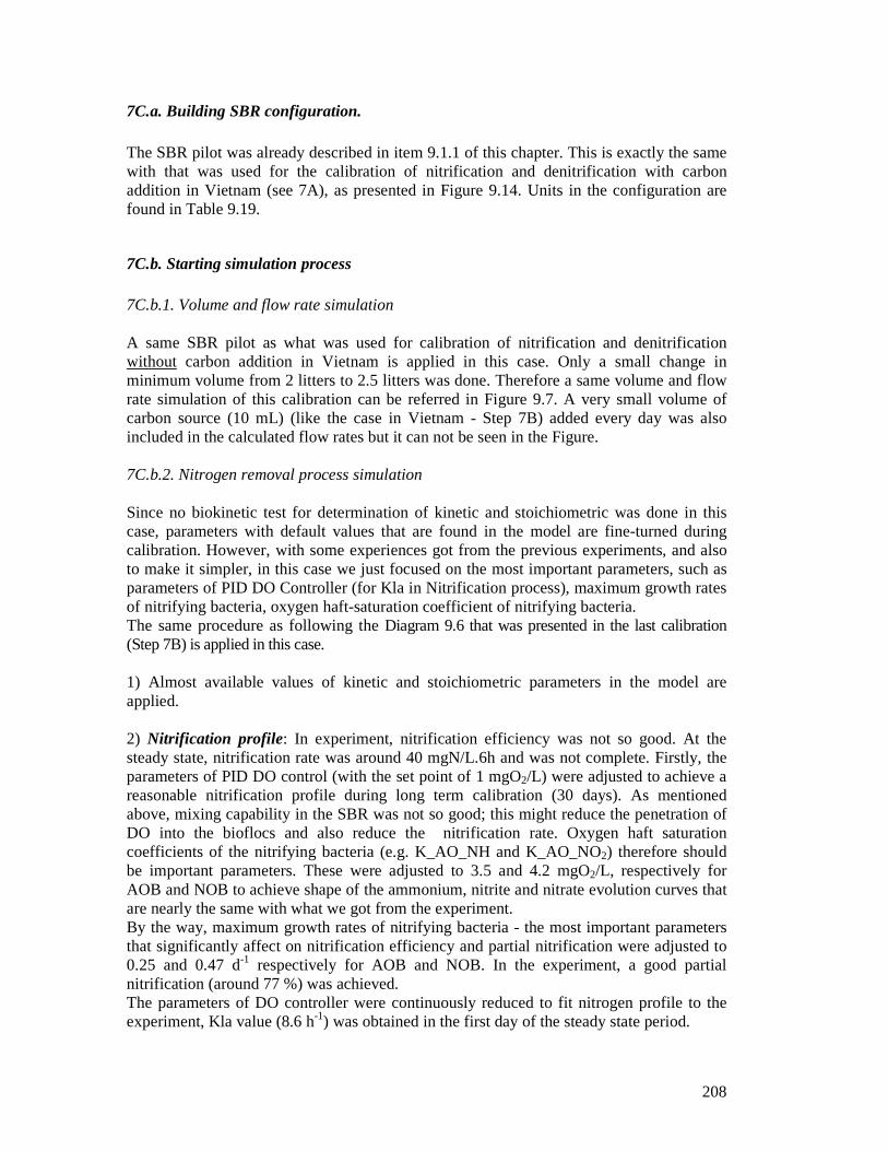
208

7C.a. Building SBR configuration. The SBR pilot was already described in item 9.1.1 of this chapter. This is exactly the same with that was used for the calibration of nitrification and denitrification with carbon addition in Vietnam (see 7A), as presented in Figure 9.14. Units in the configuration are found in Table 9.19.

7C.b. Starting simulation process 7C.b.1. Volume and flow rate simulation A same SBR pilot as what was used for calibration of nitrification and denitrification without carbon addition in Vietnam is applied in this case. Only a small change in minimum volume from 2 litters to 2.5 litters was done. Therefore a same volume and flow rate simulation of this calibration can be referred in Figure 9.7. A very small volume of carbon source (10 mL) (like the case in Vietnam - Step 7B) added every day was also included in the calculated flow rates but it can not be seen in the Figure. 7C.b.2. Nitrogen removal process simulation Since no biokinetic test for determination of kinetic and stoichiometric was done in this case, parameters with default values that are found in the model are fine-turned during calibration. However, with some experiences got from the previous experiments, and also to make it simpler, in this case we just focused on the most important parameters, such as parameters of PID DO Controller (for Kla in Nitrification process), maximum growth rates of nitrifying bacteria, oxygen haft-saturation coefficient of nitrifying bacteria. The same procedure as following the Diagram 9.6 that was presented in the last calibration (Step 7B) is applied in this case. 1) Almost available values of kinetic and stoichiometric parameters in the model are applied. 2) Nitrification profile : In experiment, nitrification efficiency was not so good. At the steady state, nitrification rate was around 40 mgN/L.6h and was not complete. Firstly, the parameters of PID DO control (with the set point of 1 mgO2/L) were adjusted to achieve a reasonable nitrification profile during long term calibration (30 days). As mentioned above, mixing capability in the SBR was not so good; this might reduce the penetration of DO into the bioflocs and also reduce the nitrification rate. Oxygen haft saturation coefficients of the nitrifying bacteria (e.g. K_AO_NH and K_AO_NO2) therefore should be important parameters. These were adjusted to 3.5 and 4.2 mgO2/L, respectively for AOB and NOB to achieve shape of the ammonium, nitrite and nitrate evolution curves that are nearly the same with what we got from the experiment. By the way, maximum growth rates of nitrifying bacteria - the most important parameters that significantly affect on nitrification efficiency and partial nitrification were adjusted to 0.25 and 0.47 d-1 respectively for AOB and NOB. In the experiment, a good partial nitrification (around 77 %) was achieved. The parameters of DO controller were continuously reduced to fit nitrogen profile to the experiment, Kla value (8.6 h-1) was obtained in the first day of the steady state period.

209

The concentration of NH4+ in the inlet leachate of around 100 mgN/L, and at the beginning

of the first cycle of steady state was around 77 mgN/L, the NH4+ at the end of this cycle

was around 33 mgN/L. During 30 days of calibration, steady state was reached at the day of 16th. Figure 9.24 and 9.25 present the nitrification profile and DO profile obtained from the calibration process.

Figure 9.24. Simulated Nitrification profiles in calibration 3

Figure 9.25. Simulated DO profiles in calibration3

The simulated DO concentration tends to increase gradually and even when nitrification profile reaches steady state. However the increase is not so fast since DO supply intensity

Time (day)

SB

R_N

utri

ent

s (m

g/L

)

SB

R_O

xyge

n (m

g/L

)

Time (day)

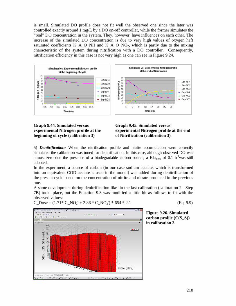
210

Simulated vs. Experimental Nitrogen profile at the beginning of cycle

0

10

20

30

40

50

60

70

80

90

100

0.25 4.25 8.25 12.25 16.25 20.25 24.25 28.25

Time (day)

Nitr

ogen

(m

gN/L

) Sim-NH4

Sim-NO2

Sim-NO3

Exp-NH4

Exp-NO2

Exp-NO3

Simulated vs. Experimental Nitrogen profile at the end of Nitrification

0102030405060708090

1 5 9 13 17 21 25 29

Time (day)

Nitr

ogen

(m

gN/L

) Sim-NH4

Sim-NO2

Sim-NO3

Exp-Nh4

Exp-NO2

Exp-NO3

is small. Simulated DO profile does not fit well the observed one since the later was controlled exactly around 1 mg/L by a DO on-off controller, while the former simulates the “real” DO concentration in the system. They, however, have influences on each other. The increase of the simulated DO concentration is due to very high values of oxygen haft saturated coefficients K_A_O_NH and K_A_O_NO2, which is partly due to the mixing characteristic of the system during nitrification with a DO controller. Consequently, nitrification efficiency in this case is not very high as one can see in Figure 9.24.

Graph 9.44. Simulated versus experimental Nitrogen profile at the beginning of cycle (calibration 3)

Graph 9.45. Simulated versus experimental Nitrogen profile at the end of Nitrification (calibration 3)

5) Denitrification: When the nitrification profile and nitrite accumulation were correctly simulated the calibration was tuned for denitrification. In this case, although observed DO was almost zero due the presence of a biodegradable carbon source, a Klaanox of 0.1 h-1was still adopted. In the experiment, a source of carbon (in our case sodium acetate, which is transformed into an equivalent COD acetate is used in the model) was added during denitrification of the present cycle based on the concentration of nitrite and nitrate produced in the previous one. A same development during denitrification like in the last calibration (calibration 2 - Step 7B) took place, but the Equation 9.8 was modified a little bit as follows to fit with the observed values: C_Dose = (1.71* C_NO2

- + 2.86 * C_NO3-) * 654 * 2.1 (Eq. 9.9)

Figure 9.26. Simulated carbon profile (C(S_S)) in calibration 3

Time (day)

SB

R_C

(S_S

) (m

g/L

)

211

Simulated vs. Experimental DO profile in cycle Cycle 40th (day 20th)

-1.0

-0.5

0.0

0.5

1.0

1.5

2.0

2.5

3.0

20.0

20.0

20.120

.120

.220.2

20.220

.320.3

20.420

.420

.420.5

Time (hour)

DO

(m

gO2/

L)

0 3 6 9 12

Sim-DO

Exp-DO

Simulated vs. Experimental Nitrogen profile in cycl eCycle 40th (day 20th)

-10

0

10

20

30

40

50

60

70

80

20 20

20.1

20.1

20.2

20.2

20.2

20.3

20.3

20.4

20.4

20.4

20.5

Time (hour)

Nitr

ogen

(m

gN/L

)

Sim-NH4

Sim-NO2

Sim-NO3

Exp-NH4

Exp-NO2

Exp-NO3

Nitrification Denitr Settling

Simulated vs. Experimental added C(S_S) in calibrat ion with carbon addition

0

50

100

150

200

250

1.264.26

7.26

10.26

13.2616

.2619.26

Time (day)

C(S

_S) (

mg

O2/

L)

Sim-addedC(S_S)Exp-added

Simulated vs. Experimental Nitrogen profile at the end of Denitrification

010203040

5060708090

0.34 4.34 8.34 12.34 16.34 20.34 24.34 28.34

Time (day)

Nitr

oge

n (m

gN/L

) Sim-NH4

Sim-NO2

Sim-NO3

Exp-NH4

Exp-NO2

Exp-NO3

Since there is not much nitrite and nitrate produced at the end of nitrification, therefore denitrification rate was much increased compared to the calibration 2. Another important model parameter relating to denitrification, n_NO was increased to its maximum value of 1 to get a better denitrification rate. Only by changing Y_STO_NO from 0.8 as default value to 0.77 could bring about a complete denitrification rate during the anoxic phase. As consequence, SND in the nitrification of the next cycles also reduced.

Graph 9.46. Simulated versus experimental carbon (C(S_S)) profile in calibration 3

Graph 9.47. Simulated versus experimental Nitrogen profile at the end of denitrification (calibration 3)

Cycle calibration: Since calibration of nitrification evolution was already good, there is no adjustment in this case but still brings about a good fit of observed and simulated data. However, oxygen profiles are not fitted very well with each other as explained above.

Graph 9.48. Simulated versus experimental Nitrogen profile in the cycle 40th (calibration 2)

Graph 9.49. Simulated versus experimental DO profile in the cycle 40th (calibration 2)

212

Step 8C. Validation with carbon addition The validation process consists in using the calibrated model with a different set of data. In this period, a twenty day simulation was run applying two different influents (one from day 1st to day 6th and the other from day 7th to day 20th). Oxygen supply intensity was increased during the first stage (day 1-6) when NH4 concentration in inlet leachate was higher (~ 210 mgN/L) then it was turned back to same level of calibration during the last stage (day 7-20). The other parameters in the operating procedure (volume etc,) were kept equal as in the calibration period. Temperature during this period did not change very much so we can consider this simulation is in a good condition regarding to the temperature. Figure 9.27 presents Nitrification profile (including ammonium, nitrite, nitrate and oxygen trends) obtained from the validation period. Figure 9.28 presents DO profile in the validation period. Graph 9.50 and 9.51 present simulated and experimental Nitrogen profiles at the end of nitrification and at the end of denitrification in the validation period.

8C.a. Validation at steady state

Figure 9.27. Simulated Nitrification profile in validation 3

SB

R_N

utri

ent

s (m

g/L

)

Time (day)

213

Simulated vs. Experimental Nitrogen profile at the end of Nitrification

0

50

100

150

200

250

1 4 7 10 13 16 19

Time (day)

Nitr

ogen

(m

gN/L

) Sim-NH4

Sim-NO2

Sim-NO3

Exp-Nh4

Exp-NO2

Exp-NO3

Simulated vs. Experimental Nitrogen profile at the end of Denitrification

0

50

100

150

200

250

0.34 3.34 6.34 9.34 12.34 15.34 18.34

Time (day)

Nitr

oge

n (

mg

N/L

) Sim-NH4

Sim-NO2

Sim-NO3

Exp-NH4

Exp-NO2

Exp-NO3

Figure 9.28. Simulated oxygen profile in validation 3

Graph 9.50. Simulated versus experimental Nitrogen profile at the end of nitrification (validation 3)

Graph 9.51. Simulated versus experimental Nitrogen profile at the end of denitrification (validation 3)

Time (day)

SB

R_O

xyge

n (m

g/L

)

214

Simulated vs. Experimental Nitrogen profile in cycl eCycle 33 th (day 16 th)

-20

0

20

40

60

80

100

120

140

16 16

16.1

16.1

16.2

16.2

16.2

16.3

16.3

16.4

16.4

16.4

16.5

Time (hour)

Nitr

ogen

(m

gN/L

)

Sim-NH4

Sim-NO2

Sim-NO3

Exp-NH4

Exp-NO2

Exp-NO3

Nitrification Denitr Settling

8C.b. Validation for a cycle

Graph 9.52. Simulated versus experimental Nitrogen profile in the cycle 16th validation 3)

Graphs 9.42 presents result obtained from cycle measurements (cycle 16th) in the validation period, showing a good fit between the simulated and experimental values for the nitrogen compounds. RESULTS OF CALIBRATION AND VALIDATION IN CASE OF CA RBON ADDITION - BELGIUM (FOR 8C) In Table 9.24, kinetic, stoichiometric and Kla values obtained during calibration and validation are presented. * Values varied with temperature

Table 9.24. Kinetic, stoichiometric and Kla values of calibration and validation period

This study – ASM3_2step

Parameters Unit Default ASM3

Model

Literature (Henze et al.,

1999; Henze et al., 2002) (20oC)

Calibration and Validation

K_A_O_NH mgCOD/L 0.75 3.5 K_A_O_NO2 mgCOD/L 1 4.2 µ_A_NH d-1 0.6 0.25 µ_A_NO2 d-1 0.7 0.47 Y_STO_NO mgCOD/mgCOD 0.8 0.43 n_NO - 0.6 1 Kla react 1 h-1 - - 8.6/

215

CONCLUSIONS OF CALIBRATION AND VALIDATION IN CASE O F CARBON ADDITION - BELGIUM (FOR 8C) Generally, modeling for one process can be implemented when the system is considered as perfectly mixed. In this case, the mixing was probably insufficient during nitrification which could reduce total nitrogen removal efficiency by reducing the penetration capacity of oxygen into the biofocs. However, low nitrification efficiency also could be due to several reasons, such as low biomass concentration and activity, characteristics of leachate (more toxic with high concentration of organic compounds, more heavy metals for example). Temperature can be a reason but if compared with the average temperature (~ 20oC) during last calibration time in case of no carbon addition (7A), the influence is not significant. Alkalinity concentration of the studied leachate is not as high as in cases 7A and 7B, in this case, average ratio of alkalinity/ammonium was just about 5.8 (mgCaCO3/mgN) but thanks for high pH (around 8.1), a good partial nitrification was still achieved (around 77%). When degradable carbon was available, denitrification was always complete, especially when there were not much nitrite and nitrate. In this case, only some main parameters were adjusted during calibration period, the simulated values seemed to be fit with the observed ones. However, low values of variables, particularly nitrite and nitrate (not more than 45 mgN/L) in both nitrification and denitrification, can reduce significantly the accuracy of the calibration process.

9.3.5. STAGE V: SCENARIO ANALYSIS AND OPTIMIZATION

Step 9A. Scenario analysis The scenario analysis for nitrification and denitrification process in case of no carbon addition was done for two different data sets of operating conditions. Parameters of working condition that are changed including working volume (leading to HRT), working time (nitrification time/denitrification time) and aeration intensity A series of experiments for each simulated scenario were implemented to verify result of simulation. The scenario analysis and its experiments were done right after the validation period so all the kinetic and stoichiometric parameters obtained after validation were applied. Inlet leachate used for this period was also the same than for validation. The simulation for scenario analysis was run for 10 days and the day where almost the experimental data are taken for comparison is day 6th. In fact these experiments can be considered as batch. The simulated data and experimental data of ammonium and nitrite evolution fit well, but not the nitrate evolution. This may be due to analytical error when nitrate concentration is low and/or the simulation demonstrates sensitivity to non fitted parameters. In fact, the experimental data of the nitrate profile are always a little bit higher than simulated ones. The experimental and simulated profiles of nitrite accumulation, however, are not very much influenced since the concentration of nitrite is always much higher than the one of nitrate. The first scenario analysis was done with different working volume and intensity of DO supply with the same operating time schedule in the cycle (6hDe – 2hNi). The second one was done with different working volumes and working time mechanism in the cycle and

216

NH4 evolution in SBR with different operating condi tion with the same DO intensity

0

50

100

150

200

250

300

350

400

6.51 6.58 6.65 6.72 6.79 6.86 6.93 7

Time (h)

NH

4 (m

gN/L

)

0

50

100

150

200

250

300

350

4000 2 4 6 8 10 12

Sim 6Ni-2De-V6LSim 5Ni-3De-V6LSim 4Ni-4De-V6LSim 6Ni-2De-V7LSim 5Ni-3De-V7LSim 4Ni-4De-V7LSim 6Ni-2De-V8LSim 5Ni-3De-V8LSim 4Ni-4De-V8LExp 6Ni-2De-V6LExp 5Ni-3De-V6LExp 4Ni-4De-V6LExp 6Ni-2De-V7LExp 5Ni-3De-V7LExp 4Ni-4De-V7LExp 6Ni-2De-V8LExp 5Ni-3De-V8LExp 4Ni-4De-V8L

NO2 evolution in SBR with different operating condi tion with the same DO intensity

0

50

100

150

200

250

300

350

6.51 6.58 6.65 6.72 6.79 6.86 6.93 7

Time (h)

NO

2 (m

gN/L

)

0

50

100

150

200

250

300

350

0 2 4 6 8 10 12

Sim 6Ni-2De-V6LSim 5Ni-3De-V6LSim 4Ni-4De-V6LSim 6Ni-2De-V7LSim 5Ni-3De-V7LSim 4Ni-4De-V7LSim 6Ni-2De-V8LSim 5Ni-3De-V8LSim 4Ni-4De-V8LExp 6Ni-2De-V6LExp 5Ni-3De-V6LExp 4Ni-4De-V6LExp 6Ni-2De-V7LExp 5Ni-3De-V7LExp 4Ni-4De-V7LExp 6Ni-2De-V8LExp 5Ni-3De-V8LExp 4Ni-4De-V8L

with the same intensity of DO supply. Concentration of activated sludge (SS) and sludge age SRT were kept stable. Hydraulic and biological parameters of the SBR were presented above in Table 9.1. Working parameters of the SBR pilot. For each scenario analysis, evolution of NH4

+, NO2-, NO3

-, AUR, NPR1, NPR2 and ratio of nitrite accumulation NO2

-/(NO2- + NO3

-) was determined. The analysis and comparison of the results between scenarios make it possible to conclude in which working condition the best nitrogen removal efficiency and the best nitrite accumulation would be obtained.

9A.a. Different working volume and working time mechanism in the cycle with the same intensity of DO supply The intensity of DO supply (DO5) used for the calibration without carbon addition was applied for this case. Parameters of the Controller were kept equal to those used for calibration. Working conditions of the SBR including working volume and time for nitrification and denitrification were changed according to each simulation scenario. Working volume includes 6, 7 and 8 litters (e.g. V6L, V7L, and V8L respectively). Working time mechanism includes 6 hours of nitrification / 2 hours of denitrification; 5 hours of nitrification / 3 hours of denitrification and 4 hours of nitrification / 4 hours of denitrification (e.g. 6Ni-2De, 5Ni-3De, and 4Ni-4De respectively). It is also noted that, Kla values for different working volume are different. The simulated values of nitrogen profile versus experimental ones are presented in Graphs 9.53. – 9.59. Note that the experimental values in the settling phase were taken as the values at the end of anoxic react phase.

Graph 9.53. Ammonium evolution in SBR with different operation conditions with the same DO supply intensity

Graph 9.54. Nitrite evolution in SBR with different operation conditions with the same DO supply intensity

217

Simulated NO2 Accumulation vs Experimental NO2 Accu mulation in difference operating condition with the same DO intensity

0.90.910.920.930.940.950.960.970.980.99

1

6Ni-2De-V6L

5Ni-3De-V6L

4Ni-4De-V6L

6Ni-2De-V7L

5Ni-3De-V7L

4Ni-4De-V7L

6Ni-2De-V8L

5Ni-3De-V8L

4Ni-4De-V8L

Operating condition

NO

2-A

cc NO2-Acc-

Sim

NO2-Acc-Exp

NO3 evolution in SBR with different operating condi tion with the same DO intensity

0

5

10

15

20

25

6.51 6.58 6.65 6.72 6.79 6.86 6.93 7

Time (h)

NO

3 (m

gN/L

)

0

5

10

15

20

250 2 4 6 8 10 12

Sim 6Ni-2De-V6LSim 5Ni-3De-V6LSim 4Ni-4De-V6LSim 6Ni-2De-V7LSim 5Ni-3De-V7LSim 4Ni-4De-V7LSim 6Ni-2De-V8LSim 5Ni-3De-V8LSim 4Ni-4De-V8LExp 6Ni-2De-V6LExp 5Ni-3De-V6LExp 4Ni-4De-V6LExp 6Ni-2De-V7LExp 5Ni-3De-V7LExp 4Ni-4De-V7LExp 6Ni-2De-V8LExp 5Ni-3De-V8LExp 4Ni-4De-V8L

AUR-Sim vs AUR-Exp with different operating conditi on with the same DO intensity

05

1015202530354045

6Ni-2De-V6L

5Ni-3De-V6L

4Ni-4De-V6L

6Ni-2De-V7L

5Ni-3De-V7L

4Ni-4De-V7L

6Ni-2De-V8L

5Ni-3De-V8L

4Ni-4De-V8L

Operating condition

AU

R (

mgN

/L.h

)

AUR-SimAUR-Exp

NPR1-Sim vs NPR1-Exp with different operating condition with the same DO intensity

05

10152025303540

6Ni-2De-V6L

5Ni-3De-V6L

4Ni-4De-V6L

6Ni-2De-V7L

5Ni-3De-V7L

4Ni-4De-V7L

6Ni-2De-V8L

5Ni-3De-V8L

4Ni-4De-V8L

Operating condition

NP

R (

mgN

/L.h

)

NPR1-SimNPR1-Exp

NPR2-Sim vs NPR2-Exp with different operating condition with the same DO intensity

0

0.5

1

1.5

2

2.5

6Ni-2De-V6L

5Ni-3De-V6L

4Ni-4De-V6L

6Ni-2De-V7L

5Ni-3De-V7L

4Ni-4De-V7L

6Ni-2De-V8L

5Ni-3De-V8L

4Ni-4De-V8L

Operating condition

NP

R2

(mgN

/L.h

)NPR2-SimNPR2-Exp

Graph 9.55. Nitrate evolution in SBR with different operation conditions with the same DO supply intensity

Graph 9.56. Simulated vs. Experimental AUR with different operating conditions with the same DO supply intensity

Graph 9.57. Simulated vs. Experimental NPR1 with different operating conditions with the same DO supply intensity

Graph 9.58. Simulated vs. Experimental NPR2 with different operating conditions with the same DO supply intensity

Graph 9.59. Simulated vs. Experimental NO2 Accumulation with different operating conditions with the same DO supply intensity

Comments: The above results show that, with the same aeration intensity, when working volume is the same, the longer time of nitrification is, the more ammonium oxidized and the more nitrite produced, leading the higher AUR and NPR1. The best working time mechanisms is 6 hours of nitrification / 2 hours of denitrification.

218

An obvious influence on AUR and NPR1 is also recognized when the system worked with the same operating time schedule but different volumes. In this case, the ammonium oxidation and nitrite production efficiency are increased when the working volume is smaller. The best AUR and NPR1 are obtained with a working volume of 6 litters. This can be explained that, when the volume is smaller, a constant intensity of oxygen supply would increase the Kla in the system, bringing more oxygen for nitrification. Effect of changing working conditions on nitrate production is not the same than for nitrite production, although it is less obvious. The nitrite accumulation profile depends somehow on the nitrate profile; however this dependence is not as significant as the nitrite concentration. In both cases (different working volumes and different working time schedules), this ratio is always high (lowest at 93.7% for the cycle 4Ni – 4De – 6L and highest at 96.0% for the cycle 6Ni – 2 De – 8L). In the condition where the highest AUR and NPR1 are obtained (6Ni – 2De – 6L), the ratio of nitrite accumulation is 94.8%, which is already a very good value. However, it could be better to find a working condition that consumes less energy (shorter aeration time) while still obtaining AUR, NPR1 and ratio of nitrite accumulation that are good enough. Looking at the results of denitrification, compared to what we found in the calibration and validation without carbon addition, denitrification efficiency is very low, almost not observed in the Graphs. An increase of denitrification time from 2 to 4 hours improved a little bit the denitrification efficiency but not very clearly. The profiles of NUR1 and NUR2 are not presented here since they are not significant. However, in case of carbon addition, a longer denitrification time could be valuable. From these points, it can be concluded that, the working condition of the cycle with 6 hours of nitrification / 2 hours of denitrification and 6 litters (6Ni – 2De – 6L) could be the best condition when the AUR, NPR1 and ratio of nitrite accumulation are very high, only a little less than the best ones. When concentration of inlet ammonium is lower, working volume should be increased to increase treatment capacity.

9A.b. Different working volume and intensity of DO supply with the same working time mechanism in the cycle (6hDe – 2hNi) In this scenario analysis, the operating schedule of 6 hours of nitrification / 2 hours of denitrification was fixed during the whole simulation/experiment process. Three different aeration intensities were applied in this case. The first one is the same that was used in the validation period without carbon addition (called DO1), the second one is identical than in the calibration period without carbon addition (called DO5) and the last one is the average level of two above intensities (called DO3). The three working volumes are 6, 7 and 8 litters (6L, 7 L and 8L). The simulated nitrogen profile versus experimental values is presented in Graphs 9.60. – 9.66. Note that the experimental values in the settling phase taken as the value at the end of anoxic react phase.

219

NH4 evolution in SBR with different operating condi tion in cycle 6h Ni - 2h De

0

50

100

150

200

250

300

350

400

6.51 6.58 6.65 6.72 6.79 6.86 6.93 7

Time (h)

NH

4 (m

gN/L

)

0

50

100

150

200

250

300

350

4000 2 4 6 8 10 12

Sim V6L-DO5Sim V6L-DO3Sim V6L-DO1Sim V7L-DO5Sim V7L-DO3Sim V7L-DO1Sim V8L-DO5Sim V8L-DO3Sim V8L-DO1Exp V6L-DO5Exp V6L-DO3Exp V6L-DO1Exp V7L-DO5Exp V7L-DO3Exp V7L-DO1Exp V8L-DO5Exp V8L-DO3Exp V8L-DO1

NO2 evolution in SBR with different operating condi tion in cycle 6h Ni - 2h De

050

100150200250300350400450500

6.51 6.58 6.65 6.72 6.79 6.86 6.93 7

Time (h)

NO

2 (m

gN/L

)

050100150200250300350400450500

0 2 4 6 8 10 12

Sim V6L-DO5Sim V6L-DO3Sim V6L-DO1Sim V7L-DO5Sim V7L-DO3Sim V7L-DO1Sim V8L-DO5Sim V8L-DO3Sim V8L-DO1Exp V6L-DO5Exp V6L-DO3Exp V6L-DO1Exp V7L-DO5Exp V7L-DO3Exp V7L-DO1Exp V8L-DO5Exp V8L-DO3Exp V8L-DO1

NO3 evolution in SBR with different operating condi tion in cycle 6h Ni - 2h De

0

5

10

15

20

25

6.51 6.58 6.65 6.72 6.79 6.86 6.93 7

Time (h)

NO

2 (m

gN/L

)

0

5

10

15

20

25

0 2 4 6 8 10 12

Sim V6L-DO5Sim V6L-DO3Sim V6L-DO1Sim V7L-DO5Sim V7L-DO3Sim V7L-DO1Sim V8L-DO5Sim V8L-DO3Sim V8L-DO1Exp V6L-DO5Exp V6L-DO3Exp V6L-DO1Exp V7L-DO5Exp V7L-DO3Exp V7L-DO1Exp V8L-DO5Exp V8L-DO3Exp V8L-DO1

AUR-Sim vs AUR-Exp with different operating conditi on in cycle 6h Ni - 6h De

0

10

20

30

40

50

60

V6L

_DO

1

V6L

_DO

3

V6L

_DO

5

V7L

_DO

1

V7L

_DO

3

V7L

_DO

5

V8L

_DO

1

V8L

_DO

3

V8L

_DO

5

Operating condition

AU

R (

mgN

/L.h

)

AUR-SimAUR-Exp

NPR1-Sim vs NPR1-Exp with different operating condition in cycle 6h Ni - 6h De

0

10

20

30

40

50

60

V6L

_DO

1

V6L

_DO

3

V6L

_DO

5

V7L

_DO

1

V7L

_DO

3

V7L

_DO

5

V8L

_DO

1

V8L

_DO

3

V8L

_DO

5

Operating condition

NP

R (

mgN

/L.h

)

NPR1-SimNPR1-Exp

NPR2-Sim vs NPR2-Exp with different operating condition in cycle 6h Ni - 6h De

0

0.5

1

1.5

2

2.5

3

V6L

_DO

1

V6L

_DO

3

V6L

_DO

5

V7L

_DO

1

V7L

_DO

3

V7L

_DO

5

V8L

_DO

1

V8L

_DO

3

V8L

_DO

5

Operating condition

NP

R2

(mgN

/L.h

)

NPR2-SimNPR2-Exp

Graph 9.60. Ammonium evolution in SBR with different operation conditions and the same DO supply intensity

Graph 9.61. Nitrite evolution in SBR with different operation conditions and the same DO supply intensity

Graph 9.62. Nitrate evolution in SBR with different operation conditions with the same DO supply intensity

Graph 9.63. Simulated vs. Experimental AUR with different operating conditions with the same DO supply intensity

Graph 9.64. Simulated vs. Experimental NPR1 with different operating conditions with the same DO supply intensity

Graph 9.65. Simulated vs. Experimental NPR2 with different operating conditions with the same DO supply intensity

220

Simulated NO2 Accumulation vs Experimental NO2 Accumulation in different operating condition with the same

working time mechanism

0.90.910.920.930.940.950.960.970.980.99

1

V6L_D

O1

V6L_D

O3

V6L_D

O5

V7L_D

O1

V7L_D

O3

V7L_D

O5

V8L_D

O1

V8L_D

O3

V8L_D

O5

Operating condition

NO

2-A

cc NO2-Acc-

Sim

NO2-Acc-Exp

Graph 9.66. Simulated vs. Experimental NO2 Accumulation with different operating conditions with the same DO supply intensity

Comments: Notably, with the same duration of aeration time, the ammonium oxidization (AUR) and nitrite production (NPR1) are efficiently increased with the increase of aeration intensity and with the decrease of working volume. The best efficiencies are achieved when DO intensity is at highest level of DO1 and working volume at 6 litters (V6L-DO1). With the cycle of V8L - DO 5 (lowest intensity and biggest volume), the AUR and NPR1 are smallest. The influence of different working conditions on the nitrate production is less obvious. As nitrate is not much produced, thus the nitrite accumulation depends more on nitrite production rather than on nitrate production. From Graph 9.66. we can see that, although the influence of the different operating conditions on the ratio of nitrite accumulation is not as high as on AUR and NPR1, but in any cases it is very high (from 94.75% to 96.28%). With a ratio that is always good, the question is, with what working condition, can we obtain sufficient ammonium removal efficiency (e.g. AUR and NPR1) while saving energy of aeration and improving treatment capacity of the system. The cycle of V6L – DO3 or V7L – DO1 could be the best ones since with these, good AUR, NPR and ratio of Nitrite accumulation are achieved, while we can save some energy (with DO 3) or improve treatment capacity (with V7L).

Step 9B. Optimisation

9B.a. Optimisation for the process without carbon addition Right after a series of experiments for the calibration period, the SBR continued to work with the same working conditions, except the condition for oxygen. In this case, the DO controller device was enabled to keep the DO concentration in the system stable around 1 mg/L. In the day when ammonium was completely consumed, a measurement campaign was carried out. The results of this experiment are used to compare with that of the experiment we got in the last day of the calibration period, providing efficiency of the process optimization when the DO controller was enabled. In Graph 9.67, we can see that, in both cases, ammonium was completely consumed at the end of Nitrification. However in case of DO controller disabled, time for complete nitrification is only about 5 hours, which means about one hour is lost and energy (e.g. oxygen) is wasted too. The wasted oxygen also leads to another problem by continuing to oxidize nitrite to nitrate, while it is not aimed in partial nitrification. When DO controller was enabled, the oxygen supply was reduced and made the rate of nitrification a little bit lower. In case of the experiment obtained, time for a completed nitrification was about 6 hours. Nitrate was less produced in this case.

221

Optimisation experimental vs. Non-Optimisation experimental DO profile

0

2

4

6

8

10

0 1 2 3 4 5 6 7 8 9 10Time (hour)

DO

(m

gO2/

L)

Opt-Exp-DO

Exp-DO

Optimisation experimental vs. Non-Optimisation expe rimental Nitrogen profile

0

50

100

150

200

250

300

350

0 1 2 3 4 5 6 7 8 9 10 11 12

Time (hour)

Nitr

ogen

(m

gN/L

) Opt-Exp-NH4

Opt-Exp-NO2

Opt-Exp-NO3

Exp-NH4

Exp-NO2

Exp-NO3

Graph 9.67. Optimisation (DO controller enabled) experimental versus No–Optimisation (DO controller disabled) experimental Nitrogen profile in case of no carbon addition.

The Graph 9.68 presents two oxygen profiles in case of control of the process (DO controller enabled) and Non-control (DO controller disabled) that were obtained during two measurement campaigns, correlatively with the Nitrogen profiles in the Graph 9.67 above. With the DO controller enabled, DO concentration in the system is well controlled around 1 mgO2/L. Comparing with the DO profile in case of DO controller disabled, we can save a big amount of oxygen (about 51 %) as can be seen during the last hour (when nitrification was completed) in Graph 9.68.

Graph 9.68. Optimisation experimental versus No-Optimisation experimental DO profile

9B.b. Optimisation for the process with carbon addition Based on the calibrated and validated model for nitrification and denitrification with carbon addition, a simulation was implemented for a period of 20 days (as for the calibration) with a different operating time schedule of 5 hours of nitrification and 3 hours of denitrification to reduce aeration time for energy saving. The source of carbon added was reduced to utilize the long settling time when denitrification is still occurring. The others working conditions (e.g. the volume, the intensity of oxygen supply, SRT, influent leachate …) were not changed. The optimization experiments were continuously done following the operating set for simulation. The new time schedule was applied and the amount of added carbon was reduced of 3.9 % (as result of the simulation) of the amount used for the calibration, which is considered as the non-optimized process. A measurement campaign for a cycle was implemented in a day where nitrification is complete. In fact in the experiment, a complete nitrification was obtained very soon since the system was already at steady state. The

222

Optimisation Simulated vs. Optimisation Experimental DO profile in cycle 40th (20th)

-10123456789

20.0

20.0

20.1

20.1

20.2

20.2

20.2

20.3

20.3

20.4

20.4

20.4

20.5

Time (hour)

DO

(m

gO2/

L)

0 3 6 9 12

Sim-DO

Exp-DO

Optimisation Nitrogen profile vs. Non optimisation Nitrogen profile in cycle Cycle 40th (day 20th)

0

50

100

150

200

250

300

350

20 20.1 20.2 20.3 20.4 20.5 20.6 20.7 20.8 20.9

Time (hour)

Nitr

ogen

(m

gN/L

)

Sim-NH4

Sim-NO2

Sim-NO3

Opt_Sim-NH4

Opt_Sim-NO2

Opt_Sim-NO3

Exp-NH4

Exp-NO2

Exp-NO3

Opt_Exp-NH4

Opt_Exp-NO2

Opt_Exp-NO3

Nitrification Denitr Settlingreduce 1 h increase 1 h

experimental data day is 20th. Comparison between the two data sets (“optimized “and non optimized process provides images and expected efficiency of the process optimization. The Graphs 9.69 presents the optimized nitrogen profile (ammonium, nitrite and nitrate) versus non optimization nitrogen profile at steady state (cycle 40th).

Graph 9.69. Optimised versus non optimised nitrogen profile in cycle

In the graph, both optimized and non-optimized ammonium profiles are almost the same, the nitrification is completed after 5 hours. That means, in the cycle of 6 hours of nitrification, 1 hour is lost as well as aeration energy if oxygen is still supplied. Saving 1 hour is not only to save aeration energy but also to avoid an amount of nitrate produced from nitrite oxidation. This could be an advantage for the efforts to a maximum partial nitrification. Looking at nitrite profiles, with one more hour for denitrification, nitrite is still well reduced even if the amount of added carbon is lower, taking advantage of the settling time where the remaining nitrite will be reduced. The percentage of carbon source saved in this case is 3.9% (simulated data) and 5.8% (experimental data). Efficiency of the optimization is also expressed though the oxygen profile. Graph 9.70 presents the simulated DO profile which fits well with the experimental DO profile.

Graph 9.70. Simulated versus experimental DO profile in an optimized cycle.

223

Optimisation Simulated DO vs. Simulated DO

01

23

45

67

20.01 20.11 20.21 20.31 20.41

Time (h)

DO

(mgO

2.L)

Sim-DO

Opt-Sim-DO

Optimisation Experimental DO vs. Experimental DO

0123456789

0 3 6 9 12

Time (h)

DO

(m

gO

2/L)

Exp-DO

Opt-Exp-DO

The Graphs 9.71. and 9.72 present the DO profile in the optimized cycle versus the one in the correlative non-optimized cycle. Graph 9.71. Optimized simulated DO vs. non optimized simulated DO

Graph 9.72. Optimized experimental DO vs. non optimized experimental DO

In the two graphs above, it is possible to see that, in the optimized cycle, an amount of oxygen (determined by mgO2/L) was saved by subtracting the extra part of oxygen in the non-optimised curve to the part of oxygen in the optimized one. In the optimized cycle, we also can save oxygen corresponding also to an amount of energy.

9.3.6. STAGE VI: EVALUATION The average relative deviation (ARD) of ammonium, nitrite and nitrate profiles between the simulation and the experiment calculated by the Equation 9.9 (Petersen et al., 2002) are:

∑=

−=

n

1i exp,i

sim,iexp,i

X

XX

n

1ARD (Eq. 9.9)

Where Xi,exp and Xi,sim are experimental and simulated values, respectively. The ARDs of NH4

+-N, NO2--N and NO3--N concentrations in the calibrations, the

validations, and scenario analysis are presented in Table 9.25 bellows:

224

Table 9.25. Evaluation results of calibration and validation

No carbon addition

Parameter Calibration - Outlet water

Calibration - Cycle

Validation - Outlet water

Validation - Cycle

Scenario analysis - Same

DO intensity

Scenario analysis -

Same working time

mechanism NH4 0.35 0.46 0.38 0.20 0.03 0.11 NO2 0.05 0.06 0.05 0.06 0.03 0.02 NO3 0.23 0.25 0.23 0.40 0.17 0.13

Carbon addition

Param-eter

Calibr- End Ni

Calibration - End De

Calibr - added C(S-S)

Calibration - Cycle

Valid - End Ni

Valid - End De

Optim - Cycle

Optim - added

C(S-S) - Cycle

NH4 0.51 0.24 0.51 0.17 0.15 0.44 NO2 0.05 0.33 0.31 0.39 0.43 0.38 NO3 0.65 1.00 0.76 0.31 1.00 0.52

C(S-S) 0.30 0.08

Notably, the smaller ARD is, the better the simulated data fit the experimental data. Some values of ARD of NH4

+ are not so good, the reason of this problem is when the value of NH4

+ concentration is small (normally at the end of nitrification process), only a small difference between the two set of data can causes a large ARD, leading to a high ARD for the whole process. If we took values above ten, the ARDs would be much smaller. The ARDs of nitrite in case of no carbon addition are always good since the value of the nitrite concentration in the whole cycle is high. In case of carbon addition, when nitrite was well reduced at the end of denitrification, there was the same problem as with ammonium at the end of nitrification. The ARDs of nitrate are not so good since the concentration this state variable is always low, a small error in analytical data also can bring about a large ARD. The evaluation through the ARD therefore is relative; the results of the calibration and validation should be based on the evolution of whole process. Further fittings will be done but we consider that those results can already be used to simulate the system to optimize the process.

225

REFERENCES:

1. Anthonisen, A. C., R. C. Loehr, T. B. Prakasam, and E. G. Srinath, 1976, Inhibition of nitrification by ammonia and nitrous acid: J. Water Pollut. Control Fed., v. 48, p. 835-852.

2. Féray, C., 2000, Nitrification en sédiment d'eau douce : incidence de rejets de station d'épuration sur la dynamique de communautés nitrifiantes, Université Lyon I, France., 204 p.

3. Gujer, W., M. Henze, T. Mino, and M. van Loosdrecht, 1999, Activated Sludge Model No. 3: Water Science and Technology, v. 39, p. 183-193.

4. HEMMIS, 2004, WEST ® WorldWide Engine for Simulation, Training and Automation - Models Guide, WEST 3.7.1.

5. HEMMIS.COM, 2004, http://www.hemmis.com/products/west/default_west.htm. 6. Henze, M., W. Gujer, T. Mino, T. Matsuo, M. C. Wentzel, G. v. R. Marais, and M.

C. M. Van Loosdrecht, 1999, Activated Sludge Model No.2d, ASM2d: Water Science and Technology, v. 39, p. 165-182.

7. Henze, M., P. Harremoes, J. L. C. Jansen, and E. Arvin, 2002, Wastewater Treatment: Biological and Chemical Processes: ISBN 3-540-42228-5, Springer - Verlag Berlin Heidelberg, Germany.

8. Henze, M., W. Gujer, T. Mino, and M. van Loosdrecht, 2000, Activated Sludge Models ASM1, ASM2, ASM2d and ASM3 in I. T. G. o. M. M. F. D. a. O. o. B. W. Treatment, ed., Scientific and Technical Report No. 9, IWA publishing, London, UK.

9. Ilenia Iacopozzi, Valentina Innocenti, Stefano Marsili-Libelli, and E. Giusti, 2007, A modified Activated Sludge Model No. 3 (ASM3) with two-step nitrificationedenitrification: Environmental Modelling & Software, v. 22 p. 847-861.

10. Metcalf&Eddy, 1991, Wastewater Engineering. Treatment, Disposal and Reuse: New York, Mc Graw - Hill Book Company. , 1771 p.

11. Patent, U., 2003, US Patent 6569334 -Method of high-concentration culture of nitrifying bacteria or denitrifying bacteria contained in activated sludge, culture promoter to be used in high-concentration culture method of nitrifying bacteria, and method of weight loss treatment of activated sludge.

12. Petersen, B., K. Gernaey, M. Henze, and P. A. Vanrolleghem, 2002, Evaluation of an ASM1 model calibration procedure on a municipal-industrial wastewater treatment plant. Hydroinformatics, v. 4, p. 15-38.

13. Tabares, L. C., 2006, Control and optimization of an SBR for nitrogen removal: From model calibration to plant operation, Universitat de Girona, Girona, 231 p.

14. http://biomath.ugent.be, BIOMATH - Department of Applied Mathematics,

Biometrics and Process control., Ghent University, Belgium. 15. http://www.stowa.nl, STOWA - The Dutch Foundation of Applied Wat. Res., The

Netherlands.

226

227

CHAPTER X: GENERAL CONCLUSIONS

It is hoped that, this study will contribute to the major issue of leachate treatment in Vietnam, especially in the North of the country where leachate characteristics and variations are the same as what was used during our experiments.

Partial nitrification seems to be easily achieved in an SBR bench-scale using leachate in Nam Son landfill site, Hanoi, Vietnam. We consider that because of the most important characteristics of the studied leachate, i.e. high alkalinity, high pH leading to high free ammonia concentration in the system. This free ammonia is known as a growth rate inhibitor for nitrite oxidizing bacteria, thus limiting oxidation of nitrite to nitrate and accumulating nitrite during the nitrification period. DO concentration is also known as an important influencing factor in partial nitrification in many previous studies. But in our case, its influence is just significant when nitrification process is nearly complete: no more ammonium remains in the system, alkalinity concentration is reduced and leading to a lower buffer capacity, lower pH, then nitrite is easily oxidized to nitrate. A sufficiently high DO concentration in this case, expresses its importance in bringing about the best nitrification efficiency, while saving aeration energy.

The SBR technique has demonstrated its advantages in this study, especially the flexibility in changing the working volume, and the operating time mechanism. The automatic SBR bench-scale used in the lab experiments has functioned very well, easy to operate and to control.

Modelisation of partial nitrification and denitrification processes for landfill leachate treatment using the Sequencing Batch Reactor technology was the main objective of this study. The simulation software - WEST® program was very useful tool to implement this task. With this program, the available model base for activated sludge model (ASM1, ASM 2, ASM 3 etc,), presented in the Peterson matrix, the variables, kinetic, stoichiometric parameters, processes can be modified easily to another activated sludge model that are suitable in the scope of our study. In the present case, based on the ASM3, the ASM3_2step was developed and applied, in which nitrification and denitrification are divided into two steps with nitrite as an intermediate product. The modified ASM3_2step has shown its high accuracy during calibration process. It could be used also for the other techniques/processes using activated sludge, not only for an activated sludge SBR by adding more equations and consequently more parameters.

Calibration and validation processes were implemented for two cases: Nitrification and denitrification with and without carbon addition in Vietnam and in Belgium. Good results were obtained where the simulations fit well the experimental data. The kinetic and stoichiometric parameters found from the calibration and validation (at steady state) are very important for the other simulations, especially in process optimisation. The process simulation is also very important in predicting the development of the treatment process. Based on the simulation profile, one can look back to the conditions of the experiments to find out if there is something wrong in the system, providing interesting tools to improve the operating conditions of the system.

It also has been demonstrated that, through scenario analysis and optimisation of the process, general productivity of the SBR system can be increased. Changing operating time cycle mechanisms by reducing the aeration time and increasing the time for anoxic phase

228

can improve the total nitrogen removal efficiency, save some energy related to aeration for nitrification and saved also the carbon source for denitrification.

The experiments were implemented in the SBR bench-scale, which is small lab equipment. It is obvious that, there will be differences when working with a real scale SBR plant, with large climate variations, with big variation of input leachate (characteristic as well as flowrate). However, the results of modelisation in this study could be a good start for simulation and optimization of an existing SBR plant (of the same type) or also for development of a new one.

As our results are very promising the next step could be to implement the ANAMMOX process. As it we now control the conditions to reach an appropriate NH4/NO2 ratio to start an ANAMMOX process.

Leachate treatment is a major issue in many countries and also in Vietnam as in other South East Asia countries where the very large pluviometry induced very large amounts of leachates but still at high concentrations.

As everywhere in the world the major issue associated to leachate treatment is the treatment of the very high fluxes of the nitrogen contained in those leachates. We demonstrated that partial nitrification can be obtained and controlled on a batch scale system which offers a rather simple and efficient way to implement leachate treatment.

Obviously the batch mode associated to the SBR process is very useful to get and to maintain the partial nitrification process, probably in a more simple and efficient way than by a continuous process.