Embed Size (px)
Citation preview

Optimization of Drift ChamberPerformance for The Qweak
Experiment
A thesis submitted in partial fulfillment of the requirement for the degree ofBachelor of Science with Honors in Physics from the College of William and
Mary in Virginia,
by
Peyton W. Rose
Advisor: Prof. David Armstrong
Prof. Charles Perdrisat
Prof. Todd Averett
Prof. Sarah Day
Williamsburg, VAMay 2011

i
Abstract
The Qweak experiment, currently running at Jefferson Lab, uses parity-
violating electron-proton scattering to measure the weak charge of the proton.
The weak charge of the proton, Qpw, is explicity predicted by the Standard
Model of particle physics. Thus, by comparing Qweak’s experimentally deter-
mined value to the theoretically predicted value of Qpw, this experiment will
test the standard model. One component of the experimental apparatus is
a set of four vertical drift chambers, constructed at the College of William
and Mary. These drift chambers are used to track electrons in the Qweak
experiment. The research presented in this paper focuses on optimizing the
performance of these drift chambers, by analyzing how their behavior varies
with operating conditions. Optimizing the performance of these chambers
will help Qweak to keep experimental uncertainties to a minimum.

Contents
1 Introduction 2
2 The Qweak Experiment 4
2.1 Overview . . . . . . . . . . . . . . . . . . . . . . . . . . . . . . 42.2 The Weak Interaction . . . . . . . . . . . . . . . . . . . . . . . 52.3 Parity . . . . . . . . . . . . . . . . . . . . . . . . . . . . . . . 62.4 Physics of Qweak . . . . . . . . . . . . . . . . . . . . . . . . . . 82.5 Experimental Setup . . . . . . . . . . . . . . . . . . . . . . . . 102.6 Tracking System . . . . . . . . . . . . . . . . . . . . . . . . . 112.7 Region Three Drift Chambers . . . . . . . . . . . . . . . . . . 15
2.7.1 Particle Detection . . . . . . . . . . . . . . . . . . . . . 162.7.2 Data Acquisition . . . . . . . . . . . . . . . . . . . . . 172.7.3 Data Analysis . . . . . . . . . . . . . . . . . . . . . . . 19
3 Measures of Chamber Performance 22
3.1 Relative Tracking Efficiency . . . . . . . . . . . . . . . . . . . 233.2 Five Wire Efficiency . . . . . . . . . . . . . . . . . . . . . . . 253.3 Mean Average Residual . . . . . . . . . . . . . . . . . . . . . . 28
4 Results 30
4.1 High Voltage Studies . . . . . . . . . . . . . . . . . . . . . . . 324.1.1 Relative Tracking Efficiency . . . . . . . . . . . . . . . 324.1.2 Five Wire Efficiency . . . . . . . . . . . . . . . . . . . 354.1.3 Average Residual . . . . . . . . . . . . . . . . . . . . . 374.1.4 Discussion . . . . . . . . . . . . . . . . . . . . . . . . . 39
4.2 Threshold Voltage Studies . . . . . . . . . . . . . . . . . . . . 404.2.1 Relative Tracking Efficiency . . . . . . . . . . . . . . . 414.2.2 Five Wire Efficiency . . . . . . . . . . . . . . . . . . . 434.2.3 Average Residual . . . . . . . . . . . . . . . . . . . . . 444.2.4 Discussion . . . . . . . . . . . . . . . . . . . . . . . . . 46
4.3 Beam Current Studies . . . . . . . . . . . . . . . . . . . . . . 47

CONTENTS iii
4.3.1 Relative Tracking Efficiency . . . . . . . . . . . . . . . 484.3.2 Five Wire Efficiency . . . . . . . . . . . . . . . . . . . 504.3.3 Average Residual . . . . . . . . . . . . . . . . . . . . . 514.3.4 Discussion . . . . . . . . . . . . . . . . . . . . . . . . . 52
4.4 Future Work . . . . . . . . . . . . . . . . . . . . . . . . . . . . 53
5 Conclusion 55
6 Bibliography 57

List of Figures
2.1 e− p Scattering . . . . . . . . . . . . . . . . . . . . . . . . . . 52.2 Parity Operation . . . . . . . . . . . . . . . . . . . . . . . . . 72.3 Particle Handedness . . . . . . . . . . . . . . . . . . . . . . . 82.4 Running of sin2(�w) . . . . . . . . . . . . . . . . . . . . . . . . 92.5 Basic Layout of Qweak Experiment . . . . . . . . . . . . . . . . 122.6 Detailed Layout of Qweak Experiment . . . . . . . . . . . . . . 142.7 Chamber Geometry . . . . . . . . . . . . . . . . . . . . . . . . 172.8 Data Collection Sequence . . . . . . . . . . . . . . . . . . . . 192.9 Tree Line Candidate . . . . . . . . . . . . . . . . . . . . . . . 21
3.1 Five Wire Efficiency Trigger . . . . . . . . . . . . . . . . . . . 26
4.1 Relative Tracking Efficiency vs. High Voltage . . . . . . . . . 344.2 Five Wire Efficiency vs. High Voltage . . . . . . . . . . . . . . 364.3 Mean Average Residual vs. High Voltage . . . . . . . . . . . . 384.4 Relative Tracking Efficiency vs. Threshold Voltage . . . . . . 424.5 Five Wire Efficiency vs. Threshold Voltage . . . . . . . . . . . 444.6 Mean Average Residual vs. Threshold Voltage . . . . . . . . . 454.7 Relative Tracking Efficiency vs. Beam Current . . . . . . . . . 494.8 Five Wire Efficiency vs. Beam Current . . . . . . . . . . . . . 514.9 Mean Average Residual vs. Beam Current . . . . . . . . . . . 52

List of Tables
2.1 List of Drift Distances for a Tree Line Candidate Event . . . . 21
4.1 List of Tracking Runs . . . . . . . . . . . . . . . . . . . . . . . 31

Chapter 1
Introduction
The Standard Model of particle physics is a theory, developed in the 1970s,
which describes the fundamental particles of nature and the electromagnetic,
strong, and weak interactions that act on these particles. To date, the Stan-
dard Model has been extremely successful in predicting experimental out-
comes, but it is known to be an incomplete theory. Among other issues, it
does not account for the gravitational force, and it requires that over twenty
of its parameters be determined from experiment. Because it is incomplete,
physicists conduct experiments to search for evidence of physics beyond the
Standard Model.
This search for new physics is conducted in two ways. High-energy ex-
periments accelerate existing particles to ultra-relativistic speeds and collide
them into each other in an attempt to generate previously unobserved forms
of matter. Any newly detected particles would need a place in future ex-
tensions of the Standard Model. At the other end of the energy spectrum,
low-energy experiments make precise measurements of values predicted by
the Standard Model. Disparities between the theoretically predicted values
and their corresponding experimental measurements would provide evidence

3
for physics beyond the Standard Model. Any future extensions of this the-
ory would be constrained by these precision measurements. The Qweak Ex-
periment is one of these low-energy, high precision experiments, currently
running at Jefferson Lab, Newport News, VA. This experiment will test the
Standard Model by making a precision measurement of the proton’s weak
charge through parity-violating electron scattering.
The purpose of the research presented in this paper was to evaluate and
optimize the performance of Qweak’s vertical drift chambers. These drift
chambers consist of two wire planes contained in a gas mixture, and are used
to track electrons in the Qweak apparatus. As elastically scattered electrons
pass through these drift chambers, their position and direction are deter-
mined. The efficiency with which scattered electrons can be detected, and
the accuracy with which their tracks can be reconstructed depend on several
operating conditions. Performance results from past tracking runs are pre-
sented, and the data will be used to optimize running conditions for future
tracking runs.

Chapter 2
The Qweak Experiment
2.1 Overview
The Qweak Experiment will use parity-violating electron-proton (e− p) scat-
tering to measure the weak charge of the proton, Qpw. In the experiment, a
polarized beam of electrons elastically scatters off of a liquid hydrogen target.
These electrons are then detected, and the results will allow for a calcula-
tion of Qpw. The goal is to test the Standard Model of particle physics by
making a precise measurement of Qpw, and comparing the theoretically pre-
dicted value to the experimentally determined value. The measurement will
be made at low four-momentum transfer (Q2) in order to minimize contri-
butions from the proton’s internal structure. The combined systematic and
statistical error in the measurement of Qpw will be 4%.
2.2 The Weak Interaction 5
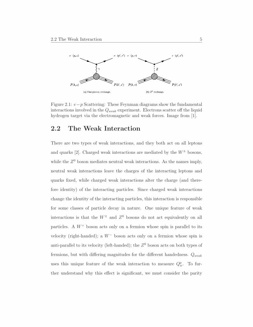
Figure 2.1: e−p Scattering: These Feynman diagrams show the fundamentalinteractions involved in the Qweak experiment. Electrons scatter off the liquidhydrogen target via the electromagnetic and weak forces. Image from [1].
2.2 The Weak Interaction
There are two types of weak interactions, and they both act on all leptons
and quarks [2]. Charged weak interactions are mediated by the W± bosons,
while the Z0 boson mediates neutral weak interactions. As the names imply,
neutral weak interactions leave the charges of the interacting leptons and
quarks fixed, while charged weak interactions alter the charge (and there-
fore identity) of the interacting particles. Since charged weak interactions
change the identity of the interacting particles, this interaction is responsible
for some classes of particle decay in nature. One unique feature of weak
interactions is that the W± and Z0 bosons do not act equivalently on all
particles. A W+ boson acts only on a fermion whose spin is parallel to its
velocity (right-handed); a W− boson acts only on a fermion whose spin is
anti-parallel to its velocity (left-handed); the Z0 boson acts on both types of
fermions, but with differing magnitudes for the different handedness. Qweak
uses this unique feature of the weak interaction to measure Qpw. To fur-
ther understand why this effect is significant, we must consider the parity

2.3 Parity 6
operator, discussed next.
2.3 Parity
In a physical process, the parity operator changes the sign of all spatial
coordinates [3]. More specifically, it will convert a right-handed coordinate
system into one that is left-handed. For example, in a three-dimensional
Cartesian coordinate system defined by unit vectors x, y, and z, a parity
operation would convert these unit vectors into -x, -y, and -z. A parity
operation is shown in Figure 2.2.
Performing this operation on a system is equivalent to observing a mir-
ror image of the physical process being studied. Originally, physicists be-
lieved that the laws of nature were invariant under such a transformation.
Experimental evidence supported this assumption for the electromagnetic
and strong interactions. However, in 1956, Lee and Yang [4] suggested that
parity-violation might occur in weak interactions. This suggestion was con-
firmed in an experiment by Wu [5], who observed the direction of emitted
electrons during the beta decay of Cobalt 60. It was found that most electrons
were emitted in the direction opposite to the nuclear spin. In a mirror image
of this process, electrons would be emitted in the direction of the nuclear
spin. However, this mirror process does not occur in nature and therefore,
the interaction does not conserve parity.
In the Qweak experiment, polarized electrons are focused onto a liquid
hydrogen target. Suppose a right-handed electron in this experiment has
momentum, p0 and spin, s0, given by s0 = r0 x p0. The spin projected onto

2.3 Parity 7
Figure 2.2: Parity Operation: This Figure shows a parity transformation,P , acting a a right-handed coordinate system, S. P transforms S into aleft-handed coordinate system, S ′.
the direction of momentum is then given by T0 = s0 ∗ p0. Performing a
parity operation on these quantities gives r′
= −r0 and p′
= −p0. Then,
s′
= −r0 x -p0 = s0. Projecting the spin onto the direction of momentum
gives T′
= s′ ∗ p′
= s0 ∗ −p0 = −T0. More simply, we find that performing
a parity operation on our right-handed electron, transforms it into a left-
handed electron. This is significant because (as discussed above) the neutral
weak interaction acts with different magnitudes on these different electrons.
Thus, the Qweak Experiment will see an asymmetry in scattering for right-
and left-handed electrons, and this asymmetry will be used to extract the
proton’s weak charge from experimental data.

2.4 Physics of Qweak 8
Figure 2.3: Particle Handedness: Here we see both a right- and left-handedparticle. Right-handed particles have their spin aligned with their momen-tum. For left-handed particles, their spin and momentum are anti-parallel.The parity operator transforms a right-handed particle into one that is left-handed.
2.4 Physics of Qweak
Physicists use the term weak charge to describe how particles ‘feel’ the weak
interaction. In the Standard Model, the weak charge of the proton is pre-
dicted [6] as
Qpw = 1− 4 sin2(�w). (2.1)
Here, �w is the weak mixing angle, which is a function of the energy at which
it is probed. This relationship between sin2(�w) and energy is shown in Figure
2.4 [6]. The blue lines gives the Standard Model prediction, while the black
points correspond to experimental results (with error bars). The red points
indicate future experiments, and are placed arbitrarily on the graph. The
size of the error bars for these future measurements gives the anticipated
uncertainty in the measurement.
To reduce corrections due to the internal structure of the proton, this
experiment will measure Qpw at low momentum transfers between the scat-
tered electrons and the proton target (Q2 = 0.03(GeV/c)2). As mentioned
above, Qweak uses parity-violating electron scattering to measure Qpw. In

2.4 Physics of Qweak 9
Figure 2.4: Running of sin2(�w): This image shows the value of sin2(�w) as afunction of energy. The Standard Model(SM) prediction is indicated by theblue line. Existing measurements [7,8,9,10] with corresponding error bars areshown in black. The red points indicate future measurements and are placedat an arbitrary location with respect to the vertical axis. Error bars for thesepoints indicate the anticipated uncertainty in the measurement.

2.5 Experimental Setup 10
particular, the scattering cross section for right- and left-handed elastically
scattered electrons will be measured. Using these quantities, we can define
an asymmetry in elastic scattering as,
ALR =�L − �R
�L + �R
, (2.2)
where �L and �R are the scattering cross sections for left- and right-handed
electrons, respectively. It can be shown from electroweak theory [6] that this
asymmetry can also be written as an expansion in Q2, given by
ALR =1
P
−GF
4��√2[Qp
wQ2 +B4Q
4 + ...]. (2.3)
Here, P is the polarization of the incident electron beam, GF is the Fermi
coupling, � is the fine structure constant, and B4 contains form factors de-
scribing the proton structure. From this equation, it is evident that for low
Q2, we can ignore the higher order terms(Q4, Q6, ...). Thus, we are left with
an equation relating the proton’s weak charge to the asymmetry in scattering
cross section, and other known and measureable quantities.
2.5 Experimental Setup
In the Qweak experiment, a 180 �A electron beam at 1.16 GeV with 85%
polarization is focused onto a 35 cm liquid hydrogen target. A series of lead
collimators is then used to select only electrons with a scattering angle of
9∘ ± 2∘, corresponding to a Q2 of 0.03 (GeV/c)2. A large toroidal magnet
is then used to further select only electrons that have scattered elastically.

2.6 Tracking System 11
These elastically scattered electrons are focused onto a set of eight quartz
Cerenkov detectors, while electrons that have scattered inelastically are bent
away from the Qweak apparatus. A schematic of the experimental setup is
shown in Figure 2.5 [6].
As the name implies, the Cerenkov detectors work on the principle of
Cerenkov radiation. When charged particles (scattered electrons in this case)
travel through a material faster than the speed of light in the medium, atoms
within the material become excited. These atoms quickly return to their
ground state and, consequently, emit radiation in the process. In Qweak’s
Cerenkov detectors, this radiation is emitted in the form of visible and UV
light (photons). Photomultiplier tubes are connected to the ends of the detec-
tors and detect the emitted photons. Data from these detectors will be used
to determine the scattering cross sections. In order to obtain results for both
right- and left-handed electrons, the beam polarization will be continuously
reversed at rates up to 960 Hz.
2.6 Tracking System
Data for the Qweak experiment will be taken in two separate modes. In pro-
duction mode, the full 180 �A current will be employed, and the asymmetry
in scattering will be measured. Periodically, the beam current will be reduced
to run the experiment in tracking mode. From equation 2.3, it is evident that
to make a precision measurement of Qpw, the momentum transfer, Q2 must be
accurately determined. For these measurements, a dedicated tracking system
has been installed in the Qweak apparatus, and is labeled by Regions 1,2, and

2.6 Tracking System 12
Figure 2.5: Basic Layout of Qweak Experiment: This image gives a side viewof The Qweak Experiment. After the electron beam scatters off the liquidhydrogen target, a series of collimators and the QTOR magnet select outonly the electrons that have elastically scattered with Q2 = 0.03 (GeV/c)2.These electrons are focused onto the quartz Cerenkov detectors.

2.6 Tracking System 13
3 in Figure 2.6 [6].
For elastic scattering, it can be shown [6] that
Q2 =4E2 sin2( �
2)
1 + 2 Emp
sin2( �2). (2.4)
Here, E is the incident beam energy, � is the scattering angle, and mp is
the mass of a proton. The incident beam energy will be measured using the
existing energy measurement system at Jefferson Lab. Thus, to calculate
Q2, we are left with the task of determining the scattering angle. The Qweak
tracking system is used to determine this scattering angle, and to ensure
that equation 2.4 is valid, by confirming that the electrons did indeed scatter
elastically.
The tracking system consists of three regions. Each of these regions will
measure the position of scattered electrons at different points within the
Qweak apparatus. Region 1 consists of gas electron multiplier chambers, and
measures the position of electrons immediately after they scatter off the hy-
drogen target. Region 2 consists of horizontal drift chambers, and measures
the position and angle of scattered electrons immediately before they en-
ter the toroidal magnet. Together, Regions 1 and 2 are used to determine
the electrons’ scattering angle. Region 3 measures the position and angle of
scattered electrons after they exit the QTOR magnet and before they enter
the Cerenkov detectors. This measurement will be used to determine the
momentum of scattered electrons, to ensure these electrons were scattered
elastically.

2.6 Tracking System 14
Figure 2.6: Detailed Layout of Qweak Experiment: Here, we see a layout ofthe Qweak apparatus, including the tracking system. The tracking system islabeled by Regions 1, 2, and 3. The mini-torus, shown here, is not used.
2.7 Region Three Drift Chambers 15
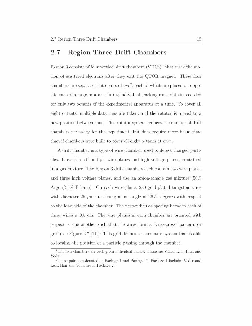
2.7 Region Three Drift Chambers
Region 3 consists of four vertical drift chambers (VDCs)1 that track the mo-
tion of scattered electrons after they exit the QTOR magnet. These four
chambers are separated into pairs of two2, each of which are placed on oppo-
site ends of a large rotator. During individual tracking runs, data is recorded
for only two octants of the experimental apparatus at a time. To cover all
eight octants, multiple data runs are taken, and the rotator is moved to a
new position between runs. This rotator system reduces the number of drift
chambers necessary for the experiment, but does require more beam time
than if chambers were built to cover all eight octants at once.
A drift chamber is a type of wire chamber, used to detect charged parti-
cles. It consists of multiple wire planes and high voltage planes, contained
in a gas mixture. The Region 3 drift chambers each contain two wire planes
and three high voltage planes, and use an argon-ethane gas mixture (50%
Argon/50% Ethane). On each wire plane, 280 gold-plated tungsten wires
with diameter 25 �m are strung at an angle of 26.5∘ degrees with respect
to the long side of the chamber. The perpendicular spacing between each of
these wires is 0.5 cm. The wire planes in each chamber are oriented with
respect to one another such that the wires form a “criss-cross” pattern, or
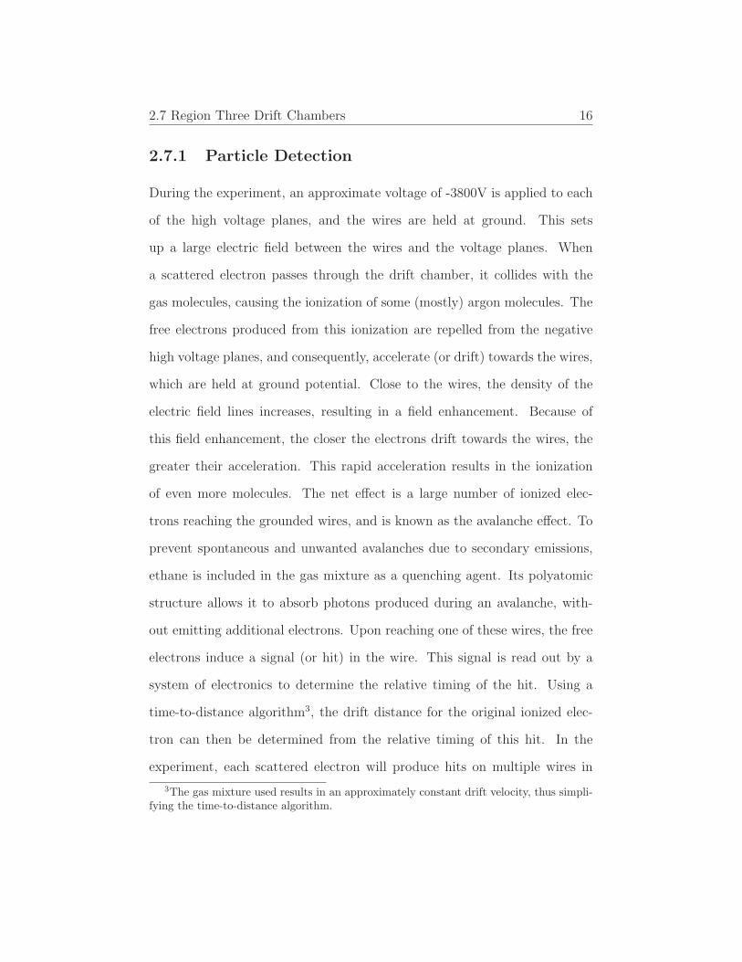
grid (see Figure 2.7 [11]). This grid defines a coordinate system that is able
to localize the position of a particle passing through the chamber.
1The four chambers are each given individual names. These are Vader, Leia, Han, andYoda.
2These pairs are denoted as Package 1 and Package 2. Package 1 includes Vader andLeia; Han and Yoda are in Package 2.
2.7 Region Three Drift Chambers 16
2.7.1 Particle Detection
During the experiment, an approximate voltage of -3800V is applied to each
of the high voltage planes, and the wires are held at ground. This sets
up a large electric field between the wires and the voltage planes. When
a scattered electron passes through the drift chamber, it collides with the
gas molecules, causing the ionization of some (mostly) argon molecules. The
free electrons produced from this ionization are repelled from the negative
high voltage planes, and consequently, accelerate (or drift) towards the wires,
which are held at ground potential. Close to the wires, the density of the
electric field lines increases, resulting in a field enhancement. Because of
this field enhancement, the closer the electrons drift towards the wires, the
greater their acceleration. This rapid acceleration results in the ionization
of even more molecules. The net effect is a large number of ionized elec-
trons reaching the grounded wires, and is known as the avalanche effect. To
prevent spontaneous and unwanted avalanches due to secondary emissions,
ethane is included in the gas mixture as a quenching agent. Its polyatomic
structure allows it to absorb photons produced during an avalanche, with-
out emitting additional electrons. Upon reaching one of these wires, the free
electrons induce a signal (or hit) in the wire. This signal is read out by a
system of electronics to determine the relative timing of the hit. Using a
time-to-distance algorithm3, the drift distance for the original ionized elec-
tron can then be determined from the relative timing of this hit. In the
experiment, each scattered electron will produce hits on multiple wires in
3The gas mixture used results in an approximately constant drift velocity, thus simpli-fying the time-to-distance algorithm.
2.7 Region Three Drift Chambers 17
Figure 2.7: Chamber Geometry: The thick black arrow represents the pathof a scattered electron as it passes through two drift chambers(one package).In this image, the grid, formed from the ”criss-cross” orientation of the wireplanes, can be seen. *Note: Distances and angles not drawn to scale.
each wire plane. The closer a scattered electron passes by a given wire, the
smaller the corresponding drift time (and drift distance). By analyzing these
drift distances for each wire, the position and angle of the scattered electrons
can be reconstructed.
2.7.2 Data Acquisition
After the ionized electrons induce a hit in each of the wires, a sophisticated
system of electronics reads out and records the data. Each wire is connected
to one channel of an amplifier/discriminator circuit board. For each chamber,
there are 36 of these circuit boards (known as MAD boards [12]). These
circuit boards have an adjustable threshold voltage. Only wire signals whose
magnitude is greater than this threshold voltage register hits on these MAD

2.7 Region Three Drift Chambers 18
boards. The output of these MAD boards is a low voltage differential signal
(LVDS) for each wire, and these signals are carried by twisted pair wires. The
next step in the data collection sequence is to convert these LVDS signals into
data that can be stored, manipulated, and analyzed on a computer. For this,
the LVDS signals are fed into a time to digital converter (TDC). These TDCs
turn an analog signal pulse into a digital representation of the time each wire
received a hit. Since the total number of wires in all four of the VDCs is 2240,
it would require 35 64-channel TDCs to handle the experimental data. To
reduce this expense, a multiplexing system [13] was implemented to reduce
the number of required TDCs to just four. In this multiplexing system, the
signals of 18 wires from separated regions of the chambers are fed into two
TDC channels along delay lines. The individual wires are then identified
by the difference of the two signals, and the drift time can be extracted by
taking the sum of the two signals. Concurrently, trigger signals are sent to
the TDC from the trigger scintillators located in front of the drift chambers.
The signals from these scintillators indicate when chamber data should be
recorded, as well as provide a reference time for the wire pulses. This entire
data acquision process is shown conceptually in Figure 2.8 [13]. All of the
wire data recorded for a single scintillator trigger is collectively referred to
as an event. These scintillators are used to reduce any noise that may make
its way onto the chamber wires. Data from the TDCs are then stored on a
computer, where it can be manipulated and analyzed using the ROOT [14]
data analysis framework.

2.7 Region Three Drift Chambers 19
Figure 2.8: Data Collection Sequence: This sequence chart gives a conceptualoverview of the data acquisition process.
2.7.3 Data Analysis
Raw data from each Qweak tracking run is stored as a file on the Jefferson Lab
computing system. This raw data is then processed by the Qweak analyzer
(essentially a data analysis program), and the output is a new data file (root
file) that can be analyzed inside the ROOT data analysis framework. Within
each root file, tracking data is organized by event number. For every event,
we can extract information about each hit in that event. This information
includes package number, wire plane number, wire number, drift time, and
drift distance for each hit. In addition to recording and organizing this basic
information, the analyzer also searches through the data file and looks for
track candidates. A track candidate is an event where the drift distances
on consecutive wires are likely to represent the path of a scattered electron.
These events are characterized by a linear relationship between drift distance
and wire position. Within ROOT, these events are labeled as “tree lines”. If
tree lines on multiple wire planes can be meshed together to fit the path of
scattered electron, this is referred to as a “partial track”. Partial tracks from
2.7 Region Three Drift Chambers 20
Regions 1, 2, and 3 are used to reconstruct the complete track of a scattered
electron.
Table 2.1 shows drift distances for each wire in a typical tree line candidate
event. These points are plotted in Figure 2.9, where the linear relationship
can be seen. Just as with individual events, the root file contains useful infor-
mation about both tree lines and partial tracks. For each of these quantities,
we can determine the wires involved (including which plane(s) and package),
the direction and slope of the fitted line, and the average residual between
the drift distance and the fitted line. ROOT is then able to make histograms
of this data, to look at general trends for entire data runs. The results pre-
sented in this paper were obtained by analyzing ROOT data for a variety of
tracking runs.

2.7 Region Three Drift Chambers 21
Wire Number Drift Distance (cm)
101 1.17102 0.58103 -0.09104 -0.57105 -1.23
Table 2.1: Here we see drift distances for each wire in a typical tree linecandidate event. When plotted the linear relationship between wire numberand drift distance can be seen.
Figure 2.9: Tree Line Candidate: Here, we see a plot of the data points givenin Table 2.1. The linear relationship between wire number and drift distancecan be observed, and therefore, this event is likely to be interpreted as a treeline candidate by the Qweak tracking analyzer.

Chapter 3
Measures of Chamber
Performance
The purpose of the research presented in the subsequent sections is to pro-
vide a quantitative analysis of Region 3 VDC performance variations with
running conditions. Since Qweak seeks to make a precision measurement of
Qpw, experimental error should be kept to a minimum. Optimizing the per-
formance of all components of the Qweak apparatus will help to keep the
combined systematic and statistical error in the measurement at or below
4%.
As evident in equation 2.3, an accurate measurement of Q2 is a vital ingre-
dient in the determination of Qpw. The ability of the Region 3 drift chambers
to track electrons will factor into this Q2 measurement. However, an exact
(mathematical) relationship between VDC performance and uncertainty in
Q2 is not available. This is due to the fact that a closed form solution of the
toroidal magnetic field does not exist. Therefore, projections of tracks from
3.1 Relative Tracking Efficiency 23
Regions 1 and 2 to Region 3 are based on computer simulations. This means
that exact relationships between VDC performance and the uncertainty in
Q2 must be determined empirically. At present, data are not available to
precisely determine these relationships. Nonetheless, we can infer that opti-
mizing the performance of the Region 3 VDCs will minimize the uncertainty
in the Q2 measurement. The research discussed below seeks to find the opti-
mal running conditions for the Region 3 VDCs. Three measures of chamber
performance are discussed, and results with respect to beam current, VDC
high voltage, and VDC threshold voltage are presented.
3.1 Relative Tracking Efficiency
One method for measuring the efficiency with which the VDCs can detect
electron tracks is to compute the relative tracking efficiency. This measure of
efficiency analyzes the performance of each entire VDC package by comparing
the number of partial tracks found in a given data run to the total number
of trigger scintillator TDC hits in that run. Mathematically, the relative
efficiency is calculated by,
Erel =npt
nf1
, (3.1)
where npt and nf11 are the total number of partial tracks and TDC hits,
respectively. In any given data run, there will be more TDC triggers than
partial tracks. This is partly due to ambient noise2 in the experimental
1“f1” refers to the specific TDC that is used for Region 3.2Including low-energy radiation present in the experimental hall.

3.1 Relative Tracking Efficiency 24
hall, and partly because the VDCs will not detect every scattered electron.
For this measure of performance, we are concerned with quantifying the
percentage of electron tracks that the VDCs detect. However, because there
is no way to distinguish the trigger scintillator signals due to noise from those
due to real electron tracks, we are forced to include both types of these signals
in our relative efficiency calculation. What this means, is that this relative
efficiency will be lower than the actual chamber efficiency. Consequently,
these results are useful for comparing chamber performance in a series of
consecutive data runs (where the level of ambient noise should be constant),
but care must be taken when comparing tracking data from different series
of runs3. Since we are assuming a constant level of noise in consecutive
data runs, any variation in the VDC relative efficiency should be due to
performance variations of the chambers, themselves.
To compare relative efficiency data from separate series of tracking runs,
we must introduce a scaling factor, �. For data taken with the same VDC
running conditions (HV and threshold) in two separate data runs (from dif-
ferent run series), � may be calculated. For these two data runs, we assume
that the chambers should have a similar level of performance, and that vari-
ations in the relative efficiency between these data runs are due to external
factors (noise, beam current, etc.). We then arbitrarily choose one of these
data runs, and calculate the relative efficiency of the VDCs. Let us denote
this efficiency as Erelbase . We will denote the efficiency of the other data run
as Erelscale . The scaling factor is then defined as
3Tracking runs are executed periodically. For runs taken weeks (or months) apart, thelevel of ambient noise will vary.
3.2 Five Wire Efficiency 25
� =Erelbase
Erelscale
. (3.2)
The relative efficiencies in the second series of data runs are then multiplied
by � to obtain the scaled relative efficiencies for that run series. The relative
efficiencies between these two series of data runs can then be compared, and
relationships in data can be inferred.
3.2 Five Wire Efficiency
A second measure of chamber performance is the five wire efficiency, which
looks at the ability of individual wires to detect particle tracks. For an
individual wire, we can define an efficiency in the following way. We let
ti denote the total number of triggers for the itℎ wire. Here, a trigger is
defined as a set of conditions that define when an individual wire should
have registered a hit. We let ℎi denote the total number of successful hits
on a given wire. A successful hit means that all trigger conditions for the itℎ
wire were met, and that wire registered a hit. The efficiency for the itℎ wire
is then given as,
Ewirei =ℎi
ti. (3.3)
In general, we are not concerned with the efficiency of one particular
wire at a time; we are concerned with how these individual wire efficiencies
change with running conditions. To investigate this behavior, we compute a
weighted sum of the efficiencies of all individual wires in a given plane (or

3.2 Five Wire Efficiency 26
Figure 3.1: Five Wire Efficiency Trigger: Here we see the trigger conditionsfor the five wire efficiency of Wire 3. Wires 1, 2, 4, and 5 must all registerhits. Additionally, the drift distance for Wire 1 must be greater than thatfor Wire 2, and the drift distance for Wire 5 must be greater than that forWire 4. For a successful fire, the same conditions are required, in additionto Wire 3 registering a hit.

3.2 Five Wire Efficiency 27
chamber, or package). This total plane efficiency is given by,
Eplane =
∑
i
ℎi
∑
i
ti(3.4)
Here,∑
i
sums over all the wires in a given plane. Similarly, to calculate
Ecℎamber and Epackage, we choose indices for all relevant wires for that sum.
In the five wire efficiency test, a trigger for Wire i requires that both pairs
of wires immediately adjacent to Wire i register a hit. However, because we
only want this efficiency test to measure a wire’s performance in detecting
tracks, we place stronger conditions on these triggers. Table 2.1 shows drift
distances for a likely track candidate. We want our five wire efficiency triggers
to select out events of this type. Thus, we require that the drift distance for
Wire i− 2 to be greater than the drift distance for Wire i− 1. Similarly, we
require the drift distance for Wire i+ 2 to be greater than the drift distance
for Wire i + 1 4. If both of these conditions are met, a trigger is registered
for Wire i. A successful fire for Wire i occurs when both of these trigger
conditions are met and Wire i registers a hit. After finding the total number
of triggers and successful fires in a given data run, the five wire efficiency can
be calculated from equation 3.3 (for an individual wire) or equation 3.4 (for
a collection of wires).
4In a ROOT file, all drift distances are given as positive values. The tracking softwaredetermines which drift distances should be negative by finding the combination that bestfits tree lines into partial tracks.
3.3 Mean Average Residual 28
3.3 Mean Average Residual
Thus far we have seen two measures of chamber performance that address
how well the VDCs can detect scattered electrons. Another measure of cham-
ber performance analyzes how well the chambers and tracking software can
reconstruct a particle track once it has been found. After a scattered elec-
tron exits the QTOR magnet, it is no longer subjected to forces that alter its
direction of motion. Thus, the scattered electrons should follow a linear tra-
jectory through the VDCs and into the Cerenkov detectors. For this reason,
we expect the Region 3 VDCs to detect straight-line particle tracks. The
tracking software is programmed to look for these straight-line tracks. For
these tracks, a linear regression model relating wire position to drift distance
can be fit to the data points. One method for evaluating how well these lin-
ear regression models fit the data points is to compute the residual for each
point. For each data point, the corresponding residual is a measure of its
distance from the linear regression fit. In other words, it is the error between
the actual drift distance, and the drift distance predicted by the linear re-
gression fit. For an individual data point, a large residual indicates the linear
regression model is not an accurate representation of that data point. For a
collection of data points and the corresponding linear regression fit, we can
consider their average residual. This average residual is given by the sum of
the magnitude of the individual residual values, divided by the total number
of data points. It is a measure of how well the linear regression model fits
the data set.
For the VDCs, the average residual is a measure of the resolution with
3.3 Mean Average Residual 29
which we can reconstruct particle tracks. A large average residual would
mean that the scattered electron passed closer or farther from the individual
wire than the model indicates. This means that we cannot be sure that
the linear regression fit gives an accurate reconstruction of the particle path.
To account for this uncertainty, we must include an associated error in the
eventual calculation of Q2. A small average residual indicates that the data
points closely follow a linear relationship. Because this is what we expect, a
small average residual allows us to infer that the drift distances are giving an
accurate measurement of the particle position. Consequently, for tracks with
small residuals, there will be a smaller associated error in the calculation of
Q2.
To evaluate the performance of the VDCs in reconstructing electron
tracks, we look at residuals for fitted tree lines. For an individual tree line,
the average residual of all data points is calculated. We then use ROOT to
make a histogram of all the average residual values in a given tracking run,
and to calculate the mean of these average residuals for all tree lines in that
run. These mean average residuals5 can then be plotted with respect to each
of the operating parameters, to determine which set of conditions gives the
best track reconstruction.
5The term “mean average residual” may sound redundant. It is important to rememberthat we are taking the mean of a collection of values, where the values are the averageresiduals for individual tree lines.
Chapter 4
Results
The results presented in this chapter are based on data from two series of
tracking runs. The first series of these runs took place over the course of
a few days in January 2011, and provide the majority of data used in the
subsequent analysis. Data from this series includes threshold, high voltage,
and beam current studies. The second series of tracking runs took place
over a few days in March 2011, and provides additional high voltage data to
supplement the January runs. Other tracking runs in March 2011 were used
to study the behavior of other components of the tracking system, and to
provide initial measurements of Q2. Table 4.1 lists the relevant tracking runs
for the VDC performance analysis, and gives the corresponding operating
conditions for each run.

31
Run Number Beam Current High Voltage (V) Threshold Voltage* (V)
8628 50 pA 3800 8.08629 50 pA 3700 8.08630 50 pA 3600 8.08631 50 pA 3900 8.08632 50 pA 3800 7.08633 50 pA 3800 6.08634 50 pA 3800 9.08635 50 pA 3800 10.08710 1.7 nA 3800 8.08713 10 nA 3800 8.08714 20 nA 3800 8.08715 30 nA 3800 8.010644 50 pA 3820 8.010645 50 pA 3720 8.010646 50 pA 3620 8.010647 50 pA 3520 8.010648 50 pA 3420 8.010649 50 pA 3320 8.010650 50 pA 3220 8.010651 50 pA 3120 8.0
Table 4.1: This table lists the tracking runs that provide the data presentedin this paper. Runs 8626-8715 were taken in January 2011 and provide datafor high voltage, threshold voltage, and beam current studies. Runs 10644-10651 were taken in March 2011 and supplement the January high voltagestudies. Note: High Voltage and Threshold Voltage refer to the Region 3operating conditions.*These are not the actual threshold values. These are the voltages suppliedto the MAD board threshold input, and are proportional to (but much largerthan) the actual threshold voltages.

4.1 High Voltage Studies 32
4.1 High Voltage Studies
The Region 3 VDCs each contain three high voltage planes. The voltage
applied to these planes directly affects the electric field inside the drift cham-
ber. Higher voltages induce higher electric fields. Consequently, the primary
ionized electrons will experience a greater acceleration towards the grounded
wires for higher voltages. This will lead to more secondary ionizations as
these electrons collides with other gas molecules (greater avalanche effect),
thus inducing a larger pulse height in the wires. The effect is that for higher
voltages, scattered electrons should be easier to detect. At the same time
however, a higher voltage means that more noise (other particles, secondary
emissions, etc.) will produce signals on the VDC wires. Therefore, optimiz-
ing the high voltage requires balancing signal detection with noise reduction.
The results in this section aim to find this optimal level of high voltage.
4.1.1 Relative Tracking Efficiency
Relative tracking efficiencies were calculated for runs 10644-10651 (March)
and runs 8628-8631 (January). In the March set of tracking runs, the beam
current was fixed at 50 pA, and the VDC threshold voltage was held constant
at 8.0 V. VDC high voltage started at 3820 V, and was lowered by 100 V
between each tracking run. For the January tracking runs, beam current and
threshold voltage were identical to the March runs, but the high voltages
ranged from 3600 V to 3900 V (in steps of 100 V). Figure 4.1 plots these
relative efficiencies vs. high voltage. In this graph, the January efficiencies
are scaled to the March efficiencies. Relative efficiencies from runs 10644 and
4.1 High Voltage Studies 33
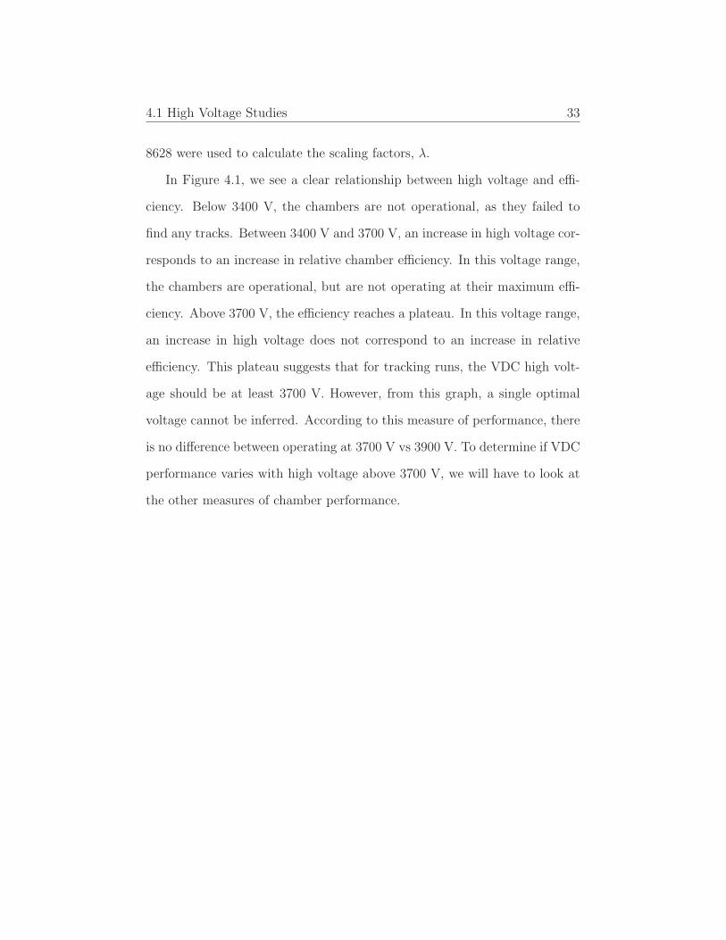
8628 were used to calculate the scaling factors, �.
In Figure 4.1, we see a clear relationship between high voltage and effi-
ciency. Below 3400 V, the chambers are not operational, as they failed to
find any tracks. Between 3400 V and 3700 V, an increase in high voltage cor-
responds to an increase in relative chamber efficiency. In this voltage range,
the chambers are operational, but are not operating at their maximum effi-
ciency. Above 3700 V, the efficiency reaches a plateau. In this voltage range,
an increase in high voltage does not correspond to an increase in relative
efficiency. This plateau suggests that for tracking runs, the VDC high volt-
age should be at least 3700 V. However, from this graph, a single optimal
voltage cannot be inferred. According to this measure of performance, there
is no difference between operating at 3700 V vs 3900 V. To determine if VDC
performance varies with high voltage above 3700 V, we will have to look at
the other measures of chamber performance.

4.1 High Voltage Studies 34
Figure 4.1: Relative Tracking Efficiency vs. High Voltage: This graph plotsVDC relative tracking efficiency as a function of high voltage. Data areincluded from the January and March 2011 tracking runs. The January datahave been multiplied by a scaling factor, so that we may compare these twosets of data on the same graph.

4.1 High Voltage Studies 35
4.1.2 Five Wire Efficiency
Results from the previous section indicate that the VDCs operate at optimal
relative efficiency for high voltages at or above 3700 V. This section looks
at the five wire efficiency of the VDCs in this voltage range. Five wire
efficiencies were calculated individually for each VDC according to equation
3.4, and results are shown in Figure 4.2.
In this graph, we see that for chambers Vader, Leia, and Han, the five
wire efficiency follows the same trend as the the relative efficiency. Between
3600 V and 3700 V, there is a significant increase in the five wire efficiency.
After this increase, the efficiency reaches a plateau for voltages at/above 3700
V. In this range, changes in high voltage do not correspond to changes in five
wire efficiency. Therefore, based on the data presented in this section, there
is an optimal range of high voltages at which the chambers can operate.
However, we still have not determined if a single high voltage optimizes
chamber performance.
This graph also shows that the behavior of the Yoda chamber differs from
the other three VDCs. Unlike the other three chambers, the Yoda chamber
does not reach an efficiency plateau for the five wire efficiency measure. Yoda
obtains a maximum efficiency at 3700 V, and this efficiency begins to decline
for higher voltages. Further research is needed to understand this different
behavior of the Yoda chamber.

4.1 High Voltage Studies 36
Figure 4.2: Five Wire Efficiency vs. High Voltage: Here, the five wire effi-ciency of each drift chamber is plotted as a function of high voltage for theJanuary 2011 tracking runs.

4.1 High Voltage Studies 37
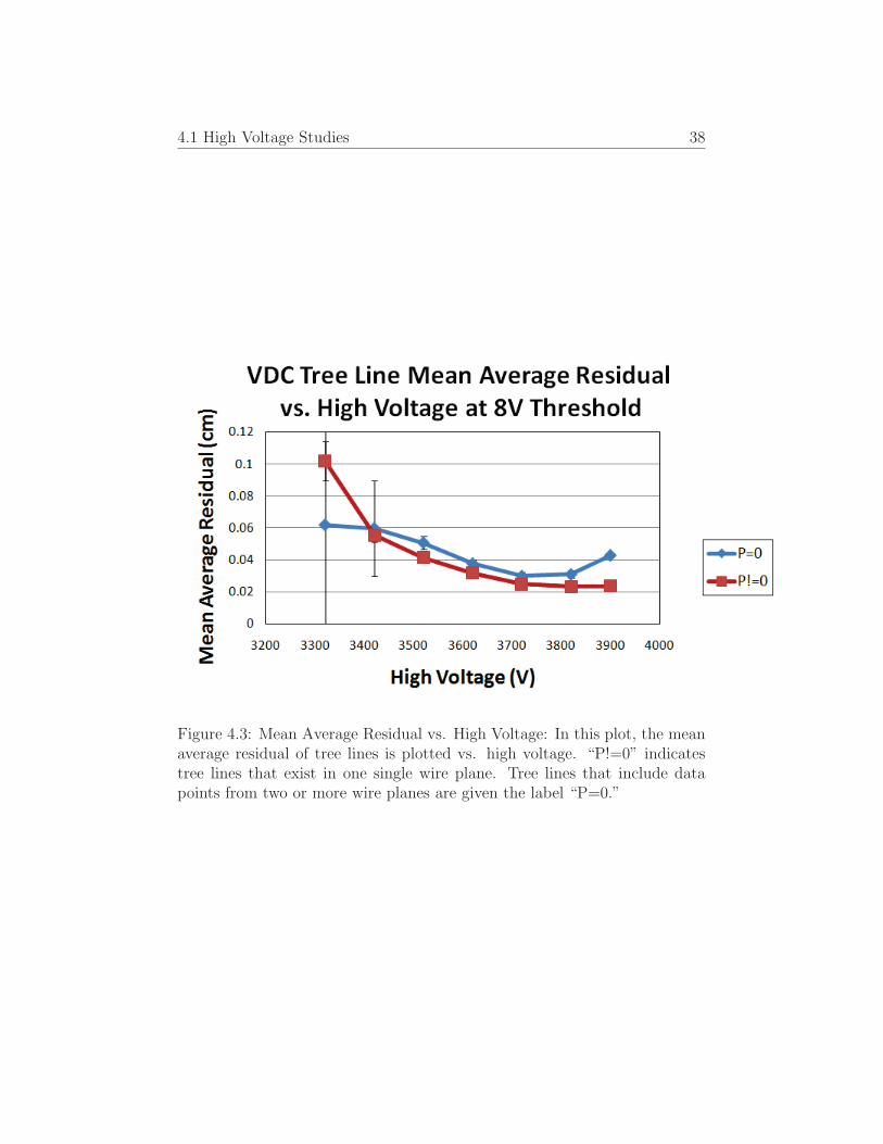
4.1.3 Average Residual
In this section, we look at how the average residual of tree lines changes with
high voltage. Data are included from both the January and March 2011
tracking runs. In this analysis, we looked at residuals from two types of tree
lines. The first is a tree line within one single wire plane. In Figure 4.3, this
data series is labeled “P!=0.” The other data series is labeled “P=0.” If the
tracking software is able to connect two tree lines from different wire planes,
the plane for this new tree line is given the value 0. This system is used to
differentiate tree lines in a single wire plane from those that are formed in
multiple wire planes.
Figure 4.3 plots the relationship between mean average residual and VDC
high voltage. We see that, between 3300 V and 3700 V, average residual de-
creases with increasing voltage. This suggests that for optimal performance,
results from these residual studies are consistent with results from both ef-
ficiency measures. The applied high voltage on the chambers should be at
least 3700 V. For single-plane tree lines, the mean average residual levels off
for voltages above 3700 V. However, for multi-plane tree lines, the mean av-
erage residual increases as the voltage is increased to 3900 V. Without more
data, it is unclear whether this is a trend that will continue. Nonetheless,
based on the data available, we can conclude that the chambers should be
operating at voltages near 3700 V and 3800 V.
4.1 High Voltage Studies 38
Figure 4.3: Mean Average Residual vs. High Voltage: In this plot, the meanaverage residual of tree lines is plotted vs. high voltage. “P!=0” indicatestree lines that exist in one single wire plane. Tree lines that include datapoints from two or more wire planes are given the label “P=0.”
4.1 High Voltage Studies 39
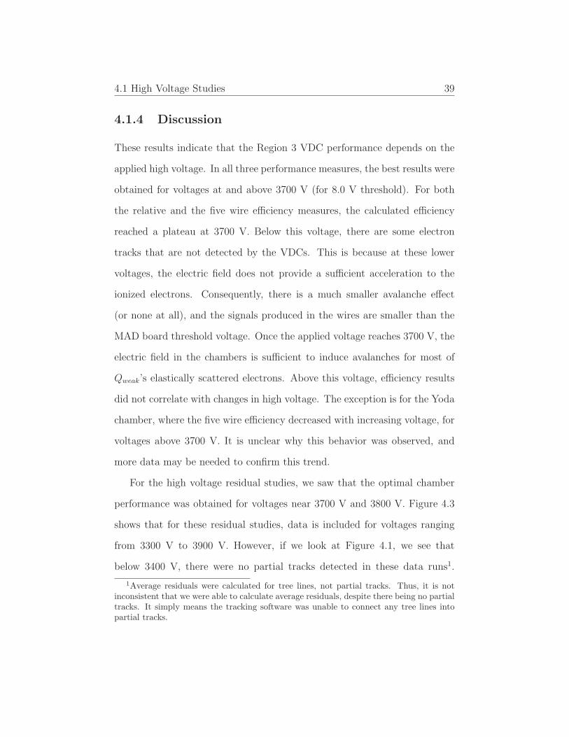
4.1.4 Discussion
These results indicate that the Region 3 VDC performance depends on the
applied high voltage. In all three performance measures, the best results were
obtained for voltages at and above 3700 V (for 8.0 V threshold). For both
the relative and the five wire efficiency measures, the calculated efficiency
reached a plateau at 3700 V. Below this voltage, there are some electron
tracks that are not detected by the VDCs. This is because at these lower
voltages, the electric field does not provide a sufficient acceleration to the
ionized electrons. Consequently, there is a much smaller avalanche effect
(or none at all), and the signals produced in the wires are smaller than the
MAD board threshold voltage. Once the applied voltage reaches 3700 V, the
electric field in the chambers is sufficient to induce avalanches for most of
Qweak’s elastically scattered electrons. Above this voltage, efficiency results
did not correlate with changes in high voltage. The exception is for the Yoda
chamber, where the five wire efficiency decreased with increasing voltage, for
voltages above 3700 V. It is unclear why this behavior was observed, and
more data may be needed to confirm this trend.
For the high voltage residual studies, we saw that the optimal chamber
performance was obtained for voltages near 3700 V and 3800 V. Figure 4.3
shows that for these residual studies, data is included for voltages ranging
from 3300 V to 3900 V. However, if we look at Figure 4.1, we see that
below 3400 V, there were no partial tracks detected in these data runs1.
1Average residuals were calculated for tree lines, not partial tracks. Thus, it is notinconsistent that we were able to calculate average residuals, despite there being no partialtracks. It simply means the tracking software was unable to connect any tree lines intopartial tracks.

4.2 Threshold Voltage Studies 40
There are two possible explanations for this. First, the fits corresponding
to electron tracks may be so poor that the tracking software is unable to
combine tree lines into partial tracks. Second, the chambers may be detecting
particles other than the experiment’s scattered electrons, such as cosmic rays,
or other sources of noise. The tracks of these particles are unlikely to have the
necessary geometry to be detected by multiple wire planes. Therefore, partial
tracks cannot be formed for these other particles. Since the chambers are
not designed to detect these particles, we expect that track reconstruction for
this noise will not be as accurate as it is for the scattered electrons. Once the
chambers are on the efficiency plateau (3700 V), the ratio of signals to noise
increases, and thus, the mean average residual at these voltages likely reflects
the resolution with which scattered electron tracks can be reconstructed.
4.2 Threshold Voltage Studies
One step in the data acquisition process is determining which wire signals
to record, and which signals to ignore. At any moment while the chambers
are in operation, there is a certain level of electronic noise on the VDC
wires. To prevent this noise from being recorded, the MAD boards have an
adjustable threshold voltage. Wire signals smaller than this threshold voltage
are ignored, while those above this threshold may be recorded. Therefore,
this adjustable threshold needs to be large enough to keep these noise signals
suppressed. If it is too high, however, some electron tracks may not be
detected on certain wires. This section looks at how the VDC performance
varies with this threshold voltage. Tracking data were recorded for threshold

4.2 Threshold Voltage Studies 41
voltages between 6.0 and 10.0 V, in 1 V increments. For these runs, there
was a 3800 V high voltage applied to the chambers, and the beam current
was fixed at 50 pA. Results for relative tracking efficiency, five wire efficiency,
and residual studies are shown below.
4.2.1 Relative Tracking Efficiency
Figure 4.4 plots VDC relative tracking efficiency as a function of thresh-
old. We see that for both packages, the relative efficiency tends to increase
with increasing threshold. For Package 1 the relative efficiency increased
by approximately 2%, and for Package 2 the relative efficiency increased by
roughly 4.5% over the range of threshold values. This increase in relative
efficiency with threshold voltage is not what is naively expected. In theory,
a lower threshold means that more particles will be detected, thus increasing
the number of partial tracks per TDC trigger. This will be addressed further
in the discussion. Additionally, this graph shows that the Package 2 relative
tracking efficiency is lower than that for Package 1. One possible explana-
tion is that, despite the same threshold voltage being applied to all chambers,
there exist some natural variations in the active threshold of the chambers.
As suggested by this graph, a lower threshold for Package 2 compared to
Package 1 may explain this disparity.

4.2 Threshold Voltage Studies 42
Figure 4.4: Relative Tracking Efficiency vs. Threshold Voltage: The graphshows the dependence of relative tracking efficiency on threshold voltage forPackages 1 and 2.

4.2 Threshold Voltage Studies 43
4.2.2 Five Wire Efficiency
The five wire efficiency of each VDC as a function of threshold voltage is
plotted in Figure 4.5. From this graph, it appears there is a slight dependence
of five wire efficiency on threshold voltage. The five wire efficiency increases
with increasing threshold voltage. However, over the entire range of threshold
values, the efficiency of three of the four chambers change by less than 1%.
The exception is the Yoda chamber, whose efficiency increases by 2% over
this range, but whose overall efficiency is well below the efficiency of the other
three chambers. Again, this increase in efficiency with threshold voltage is
not what is naively expected, and will be addressed in the discussion.

4.2 Threshold Voltage Studies 44
Figure 4.5: Five Wire Efficiency vs. Threshold Voltage: Here, the five wireefficiency of each chamber is plotted vs. threshold voltage.
4.2.3 Average Residual
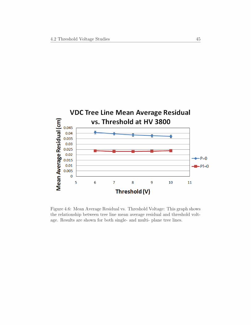
Figure 4.6 shows the variation in VDC tree line mean average residual with
threshold voltage. The results in this graph indicate that for single-plane
tree lines, the mean average residual is not affected by the threshold volt-
age. For multi-plane tree lines, the mean average residual tends to slightly
decrease with increasing threshold voltage. This suggests that higher thresh-
old voltages have little effect on the amount of noise in any individual wire
planes. However, for multi-plane events, the higher threshold voltages select
track candidates with the best resolution, thereby reducing the mean average
residual.
4.2 Threshold Voltage Studies 45
Figure 4.6: Mean Average Residual vs. Threshold Voltage: This graph showsthe relationship between tree line mean average residual and threshold volt-age. Results are shown for both single- and multi- plane tree lines.

4.2 Threshold Voltage Studies 46
4.2.4 Discussion
Results from this section provide evidence that increasing the MAD board
threshold voltage optimizes Region 3 VDC performance. We saw that both
measures of efficiency increase with increasing threshold. At the same time,
the mean average residual for multi-plane tree lines decrease with increasing
threshold. It was expected that increasing the threshold voltage would reduce
the mean average residual. This is because higher threshold voltages filter
out noise hits and signals that have the potential to negatively impact the
mean average residual.
It was mentioned in the above sections that the observed relationship
between efficiency and threshold is unexpected. The threshold voltage is
designed to filter out noise signals that would dilute relevant chamber data.
However, in the process of filtering these noise signals, the threshold will
likely throw away smaller signals from actual electron tracks. For the relative
efficiency measure, this would imply that some partial tracks, which would
be detected at lower thresholds, are filtered out at higher thresholds. Since
the number of TDC hits should be independent of the threshold voltage, we
would expect the relative efficiency to decrease.
The fact that relative tracking efficiency increases with increasing thresh-
old voltage may indicate that some noise signals are interfering with some rel-
evant chamber signals. For each event, multiple hits are sometimes recorded
for a single wire. Currently however, it is only the first hit that is used in the
data analysis. Thus, if a relevant chamber signal is immediately preceded by
a noise signal, the relevant signal may be excluded from the data analysis.

4.3 Beam Current Studies 47
In this case, chamber performance would be optimized by using a higher
threshold voltage.
For the five wire efficiency, we again saw that increasing the threshold
voltage increases the chamber efficiency. One possible explanation is that the
size of a wire pulse might be a function of how close the scattered electron
passed to the wire. If electrons induce bigger pulses in the wires they travel
closest to, then increasing threshold voltage would decrease the number of
five wire efficiency triggers in a given tracking run. This is because the
magnitude of smaller signals on Wires i − 2 and i + 2 would be less likely
surpass higher threshold voltages. Therefore, we would expect more trigger
conditions to fail than test conditions, thus increasing the five wire efficiency
of the chambers. Further research is needed to support this explanation.
4.3 Beam Current Studies
During Qweak tracking runs, the beam current is reduced from 180 �A (pro-
duction mode current) to approximately 50 pA. However, because the current
used in these tracking runs may not always be exactly 50 pA, a series of runs
was taken to study the effects of beam current on VDC performance. Data
for these runs were taken at beam currents ranging from 1.7 nA to 30 nA.
These beam currents are significantly (order-of-magnitude) greater than the
currents used in tracking runs. Nonetheless, they do provide a useful analysis
of how beam current affects chamber performance.

4.3 Beam Current Studies 48
4.3.1 Relative Tracking Efficiency
Figure 4.7 graphs VDC relative tracking efficiency vs. beam current. This
graph shows that VDC relative efficiency decreases with increasing beam
current. As the beam current increased from 1.7 nA to 30 nA, the relative
efficiency of both packages decreased by approximately 7%. It is important to
note, however, that these beam currents are significantly greater than those
used in tracking runs. Therefore, we do not expect beam current variations
to have a significant effect on VDC relative efficiency during these tracking
runs. In Figure 4.7, we also see a difference in the relative tracking efficiency
between Packages 1 and 2. However, this time (compared to Figure 4.4),
the efficiency of Package 2 is greater than the efficiency of Package 1. This
supports our assumption that this difference is due to natural variations in
running conditions (such as threshold voltage).

4.3 Beam Current Studies 49
Figure 4.7: Relative Tracking Efficiency vs. Beam Current: The graph showsthe dependence of relative efficiency on beam current. Results for Packages1 and 2 are plotted separately.

4.3 Beam Current Studies 50
4.3.2 Five Wire Efficiency
In Figure 4.8, we see a relationship between beam current and five wire effi-
ciency. As with relative efficiency, the five wire efficiency also decreases with
increasing beam current. Again however, the magnitude of beam currents
for these studies is far greater than the currents used during actual track-
ing runs. Therefore, we do not expect the beam current variations during
tracking runs to have a significant impact on the five wire efficiency of the
chambers.

4.3 Beam Current Studies 51
Figure 4.8: Five Wire Efficiency vs. Beam Current: Here, the five wireefficiency of each chamber is plotted vs. beam current. Data are from theJanuary tracking runs.
4.3.3 Average Residual
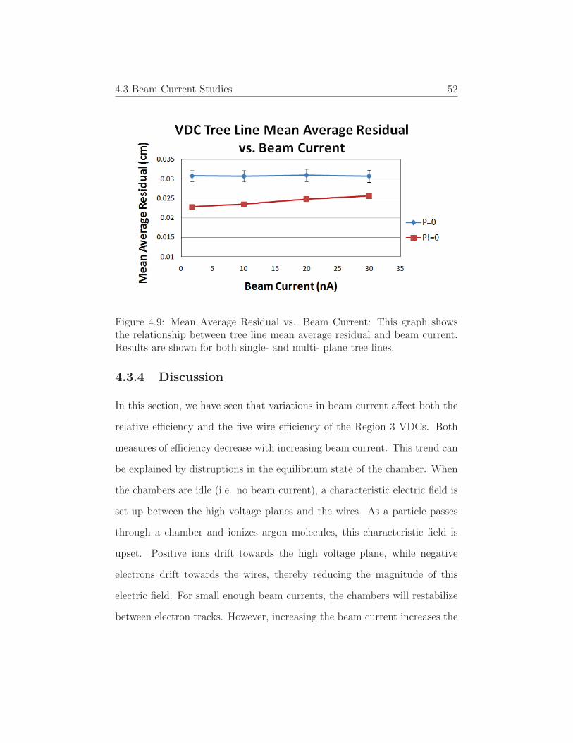
The graph in Figure 4.9 plots mean average residual as a function of beam
current. We see that for multi-plane tree lines, there does not appear to be
a relationship between these quantities. There are some slight fluctuations
in mean average residual for these multi-plane tree lines, but no definite
relationship can be inferred. For single-plane tree lines, however, there does
appear to be a small correlation between beam current and mean average
residual. Mean average residual for these single-plane tree lines appears to
increase slightly with increases in beam current. Again, we do not expect
this effect to be significant at the beam currents used for Q2 measurements.
4.3 Beam Current Studies 52
Figure 4.9: Mean Average Residual vs. Beam Current: This graph showsthe relationship between tree line mean average residual and beam current.Results are shown for both single- and multi- plane tree lines.
4.3.4 Discussion
In this section, we have seen that variations in beam current affect both the
relative efficiency and the five wire efficiency of the Region 3 VDCs. Both
measures of efficiency decrease with increasing beam current. This trend can
be explained by distruptions in the equilibrium state of the chamber. When
the chambers are idle (i.e. no beam current), a characteristic electric field is
set up between the high voltage planes and the wires. As a particle passes
through a chamber and ionizes argon molecules, this characteristic field is
upset. Positive ions drift towards the high voltage plane, while negative
electrons drift towards the wires, thereby reducing the magnitude of this
electric field. For small enough beam currents, the chambers will restabilize
between electron tracks. However, increasing the beam current increases the

4.4 Future Work 53
likelyhood that a second electron will pass through a region of the chamber,
before the chamber has restablized from the first electron. In that case, the
electric field may not be strong enough to induce an avalanche effect, and this
second scattered electron may not be detected. Therefore, both the relative
efficiency and the five wire efficiency decrease due to this effect.
We also saw that these beam current variations have little to no effect
on the mean average residual of fitted tracks. In particular, no effect was
observed on the mean average residual for multi-plane tree lines. There did
appear to be a small correlation between single-plane tree line mean aver-
age residual and beam current. Based on the discussion above, we would
not expect the residuals to increase with increasing beam current. An in-
crease in beam current affects the efficiency due to disruptions in the electric
field. However, once the characteristic electric field is restored, the chambers
should be ready to detect electrons with the same level of resolution. The
increase in average residual for single-plane tree lines is likely due to sec-
ondary particles. Increasing the beam current may increase the number of
noise particles passing through the chambers. However, due to the trajecto-
ries of these particles, it is unlikely that they would produce multi-plane tree
line events. Therefore, only the single-plane tree line residuals are affected
by these noise particles.
4.4 Future Work
The research presented in the above sections uses the data currently avail-
able to provide an overview of chamber performance variations with running

4.4 Future Work 54
conditions. Using these data, we were able to describe how chamber per-
formance varies with VDC high voltage, VDC threshold voltage, and beam
current. However, for the high voltage and threshold voltage studies, the
data available do not allow for a complete, in-depth analysis of chamber be-
havior. For the high voltage studies, we studied how the applied high voltage
affects chamber performance, at a threshold of 8 V. For a complete analysis,
we would perform the same high voltage studies at multiple threshold val-
ues. Likewise, our threshold voltage studies look at variations in chamber
performance with threshold voltage, at a high voltage of 3800 V. Further
research would perform these threshold studies at multiple high voltage val-
ues. The values 8 V and 3800 V were used because preliminary analysis of
chamber behavior suggested that these values produced a sufficient level of
chamber performance. However, this preliminary analysis was not carried
out using beam data from the experimental hall. We have already seen ev-
idence that higher threshold voltages produce higher chamber efficiencies,
and future data may indicate that other combinations of high voltage and
threshold better optimize chamber performance. The level of future research
into these questions will depend on the amount of beam time available to
perform these additional high voltage and threshold studies.
Chapter 5
Conclusion
The research presented in this paper was focused on understanding how the
Region 3 VDC performance varies with operating conditions. Chamber per-
formance was studied with respect to high voltage, threshold voltage, and
beam current. The purpose of the high voltage and threshold voltage studies
was to find the optimal running conditions for the VDCs. The data included
and the analysis that followed suggests that chamber performance is opti-
mized for high voltages near 3800 V. For voltages below 3700 V, it was clear
that the chambers were not operating at maximum efficiency. Above 3800 V,
there was some evidence that tree line residual may increase, thereby decreas-
ing track resolution. For threshold voltage, all data suggests that chamber
performance is optimized for high thresholds. Increasing threshold voltage
correlates with increasing efficiency and decreasing mean average residuals.
Further research may be necessary to determine what upper limit should be
imposed on the threshold voltage. The purpose of the beam current studies
was to ensure that chamber performance is not heavily impacted by varia-

56
tions in the tracking mode current. Data for these studies was taken with
beam currents significantly greater than those used for Q2 measurements.
It was observed that chamber performance decreases with increasing beam
current. However, these variations in chamber performance are not expected
to be of any significance at the lower current rates. Further research will look
at how variations in these (and other) running conditions directly affect the
measurements of Q2. Accurate measurements of Q2 are vital to Qweak’s goal
of making a precise measurement of the proton’s weak charge.

Chapter 6
Bibliography
[1] Humensky, T.B. Ph.D. Dissertation: Probing the Standard Model and
Nucleon Structure via Parity-Violating Electron Scattering. 2003.
[2] Griffiths, D. Introduction to Elementary Particles, 2nd ed. (Wiley-Vch,
Weinheim, 2008).
[3] Perkins, D.H. Introduction to High Energy Physics, 2nd ed. (Addison-
Wesley Publishing Company, Reading, 1982).
[4] Lee, T.D. and Yang, C.N. Phys. Rev. 104, 254 (1956).
[5] Wu, C.S. et al. Phys. Rev. 105, 1413 (1957).
[6] Armstrong et al. The Qweak Experiment: “A Search for New Physics
at the TeV Scale via a Measurement of the Protons Weak Charge.”
http://www.jlab.org/qweak/ , (Unpublished, Proposal Update to
Jefferson Lab Program Advisory Committee) 2007.
[7] Bennett, S.C. and Wieman, C.E. Phys. Rev. Lett. 82, 2484 (1999).
[8] Anthony, S.C. et al. Phys. Rev. Lett. 95, (2005).
[9] Zeller, G.P. et al. Phys. Rev. Lett. 88, (2002).
58
[10] Yao, W.M. et al. J. Phys. G33, (2006).
[11] Mitchell, J. http://hallaweb.jlab.org/document/OPMAN/node134.html.
(Accessed 14 April 2011).
[12] Rachek, I. et al. New Amplifier-Discriminator Cards for Multiwire
Drift Chambers. http://hallaweb.jlab.org.
[13] Zielinski, R.B. W&M Senior Thesis Project: Testing and Analysis of
Q-Weak’s Multiplexing Electronics System. 2010. (Unpublished)
[14] ROOT. http://root.cern.ch/drupal/.