An-Najah National University

Faculty of Graduate Studies

Optimization Models in Green Supply

Chain Management

By

Issa Asrawi

Supervisor

Dr. Yahya Saleh

Co- Supervisor

Dr. Mohammad Othman

This Thesis is Submitted in Partial Fulfillment of the Requirements for

the Degree of Master of Engineering Management, Faculty of Graduates

Studies, An-Najah National University, Nablus, Palestine.

2016

III

Dedication

Every challenging work needs effort as well as guidance of

those who are very close to our heart.

My humble effort I dedicate my thesis to my sweet and

loving

Father & Mother & Siblings

Whose affection, love, encouragement and prays of day and

night make me able to get such success and honor.

IV

Acknowledgement

I would like to express my sincere and deep gratitude to my supervisors Dr.

Yahya Saleh and Dr. Mohammad Othman for their guidance, help,

encouragement and support. Their wide knowledge, experience and

continuous support have been of great contribution to this thesis. I would

like to thank both of them for helping me in shaping, enhancing and

expanding my research skills and for everything they have done for me.

I am deeply grateful to the member of the thesis committee; Dr. Ahmad Al-

Ramahi and Dr. Suhil Sultan for devoting their valuable time to read and

review this thesis manuscript. Their suggestions, comments and

recommendations are great value to the quality of this thesis.

I would like to extend my thanks and appreciation to my instructors at An-

Najah National University, for sharing expertise, sincere, valuable

guidance and encouragement.

Finally, special thanks to my family, friends and colleagues for their

encouragement and support they gave me.

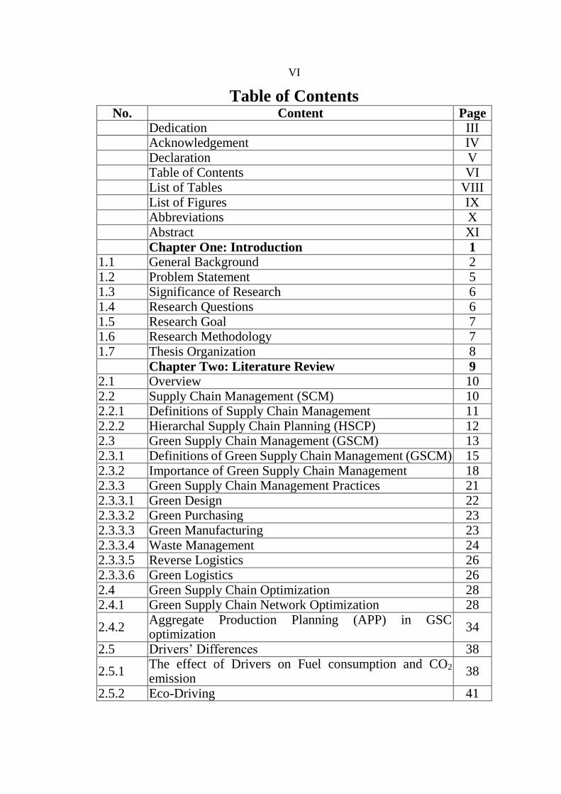
VI

Table of Contents No. Content Page

Dedication III

Acknowledgement IV

Declaration V

Table of Contents VI

List of Tables VIII

List of Figures IX

Abbreviations X

Abstract XI

Chapter One: Introduction 1 1.1 General Background 2 1.2 Problem Statement 5 1.3 Significance of Research 6 1.4 Research Questions 6 1.5 Research Goal 7 1.6 Research Methodology 7 1.7 Thesis Organization 8

Chapter Two: Literature Review 9 2.1 Overview 10 2.2 Supply Chain Management (SCM) 10 2.2.1 Definitions of Supply Chain Management 11 2.2.2 Hierarchal Supply Chain Planning (HSCP) 12 2.3 Green Supply Chain Management (GSCM) 13 2.3.1 Definitions of Green Supply Chain Management (GSCM) 15 2.3.2 Importance of Green Supply Chain Management 18 2.3.3 Green Supply Chain Management Practices 21 2.3.3.1 Green Design 22 2.3.3.2 Green Purchasing 23 2.3.3.3 Green Manufacturing 23 2.3.3.4 Waste Management 24 2.3.3.5 Reverse Logistics 26 2.3.3.6 Green Logistics 26 2.4 Green Supply Chain Optimization 28 2.4.1 Green Supply Chain Network Optimization 28

2.4.2 Aggregate Production Planning (APP) in GSC optimization

34

2.5 Drivers’ Differences 38

2.5.1 The effect of Drivers on Fuel consumption and CO2 emission

38

2.5.2 Eco-Driving 41

VII

2.6 Green Human Resources Management (GHRM) in Supply Chain Management (SCM)

47

2.7 Summary 49

Chapter Three: Model Formulation 50 3.1 Overview 51 3.2 Mixed Integer Linear Programming (MILP) 51 3.2.1 Importance of MILP in Solving GSCM Problems 53 3.3 Model Description 53 3.3.1 Assumptions 56 3.3.2 Sets 58 3.3.3 Parameters 58 3.3.4 Decision Variables 60 3.3.5 Objective Function 60 3.3.6 Total Objective Function 63 3.3.7 Constraints 63 3.4 Summary 72

Chapter Four: Model Results 73 4.1 Overview 74 4.2 Hypothetical Data 74 4.3 Results 76 4.3.1 Matlab solver and Algorithms 76 4.3.2 Numerical Results 77 4.4 Summary 84

Chapter Five: Sensitivity Analysis 85 5.1 Overview 86

5.2 Conducting Sensitivity Analysis on the GHG emission level

86

5.2.1 The Effect of GHG Emission Level on The Total Cost of SC

86

5.2.2 The Effect of GHG Emission Level on The Drivers Workforce Plan

88

5.3 Conducting Sensitivity Analysis on The Distance between DCs and Retailers

90

5.4 Conducting Sensitivity Analysis on The Cost of Drivers 94 5.5 Summary 98

Chapter Six: Conclusions and Recommendations 99 6.1 Summary 100 6.2 Contribution 102 6.3 Limitations and Recommendations 102 6.4 Future Works 103

References 105

ب الملخص

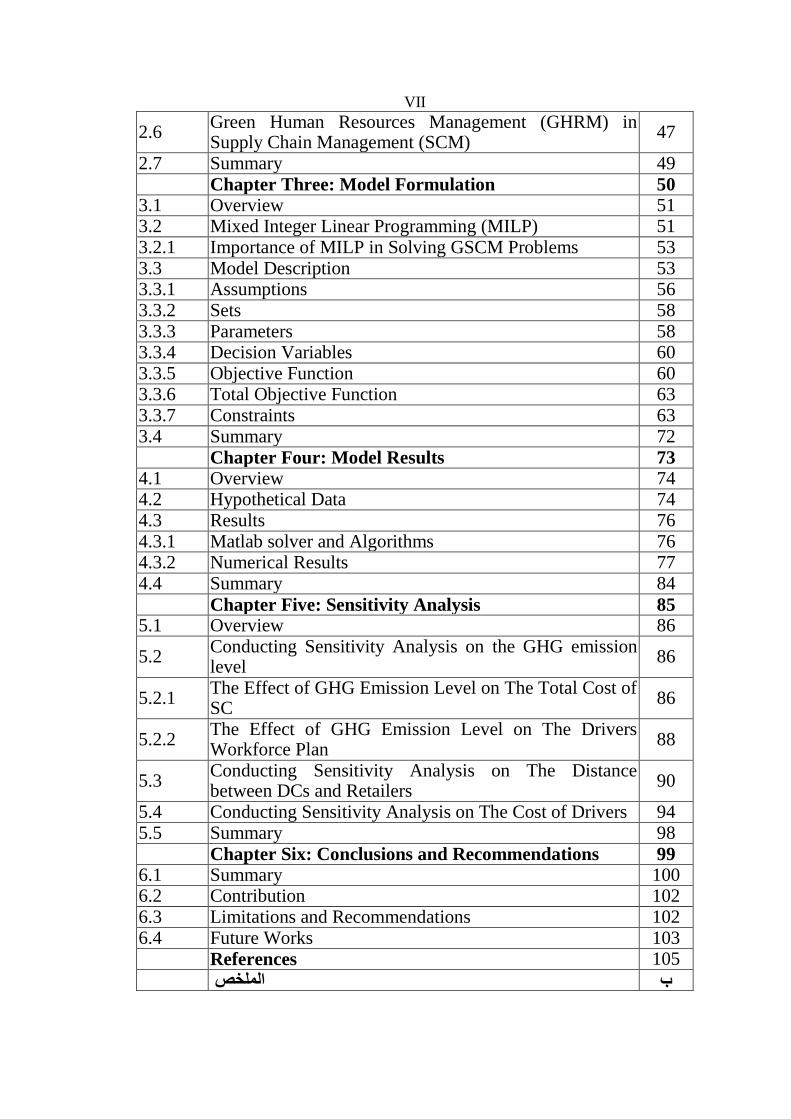
VIII

List of Tables No. Table Page

Table (2.1) The Effect of Drivers on Fuel Consumption and

CO2 Emission at Different levels 45

Table (2.2) Categories of Eco-Driving Behavior and Some of

Their Psychologically Attributes 46

Table (4.1)

Demand Forecast, Distances Between Retailers

and DCs in km, Inventory Costs and Storage

Capacities at Retailers

75

Table (4.2) Inventory Cost, Storage Capacities at DCs and

Allowable GHG Emission Level in Each Period 75

Table (4.3) Vehicles’ Data 75

Table (4.4) Workforce’ Data Cost 76

Table (4.5) Initial Drivers and Drivers’ Cost in ($/Driver) and

Their GDI 76

Table (4.6) Suppliers Data 76

Table (4.7) Workforce Plan obtained from Solving The

Proposed Model 78

Table (4.8) Drivers Plan Obtained from Solving The

Proposed Model 79

Table (4.9) Number of Vehicles g Used to Ship Products

From DC j to Retailer r 80

Table (4.10) Number of Assignments between Driver level m,

Vehicle type g and Retailer r at DC j 81

Table (4.11) The Quantities to be Shipped from Supplier k to

DC j in Period t 82

Table (4.12) The Quantities to be Shipped from DC j to

Retailer r in Period t 83

Table (4.13) Objective Function Components in ($) 83

Table (5.1) Number of assignments between driver level 𝑚,

vehicle type 𝑔 and retailer 𝑟 at DC 𝑗 in period 𝑡 93

IX

List of Figures No. Figure Page

Figure (2.1) Hierarchical Supply Chain Planning Framework 13

Figure (2.2) Process Involved in Green Supply Chain

Management 18

Figure (2.3) Activities in Green Supply Chain 22

Figure (2.4)

Model Describing factors that affect the amount

of vehicular energy use and exhaust emission

(Ericsson, 2001)

40

Figure (3.1) A Configuration of the Supply Chain Network 56

Figure (5.1) Total Cost Against GHG emission Limitation 88

Figure (5.2) The Relation Between Number of m-Level

Driver and GHG Limitation 90

Figure (5.3)

The Relation Between Number of m-Level

Driver and the Distance Between DCs and

Retailers

92

Figure (5.4)

The Effect of Differences in Cost Between

Drivers Levels on the Selection of Drivers in

DCs

96

Figure (5.5)

The Effect of Differences in Cost Between

Drivers Levels on The Selection of Drivers at

DC 1

97

Figure (5.6)

The Effect of Differences in Cost Between

Drivers’ Levels on The Selection of Drivers at

DC 2

97

X

Abbreviations GSCM Green Supply Chain Management

SC Supply Chain

GDI Green Driving Index

MINLP Mixed Integer Non Linear Programming

MILP Mixed Integer Linear Programming

GHG Greenhouse Gases

CO2 Carbon Dioxide

APP Aggregate Production Planning

GL Green Logistics

DC Distribution Center

LCA Life Cycle Assessment

GHRM Green Human Resources Management

CSCMP Council of Supply Chain Management Professionals

CLGSC Close Loop Green Supply Chain

GP Goal Programming

MOGA Multi-Objective Genetic Algorithm

LP Linear Programming

IP Integer Programming

MIR Mixed Integer Rounding

OM Operations Management

JIT Just In Time

ABC Activity Based Costing

HC Hydrocarbon

NOx Nitrogen Oxides

Eco Ecological

EPA Environmental protection Agency

XI

Optimization Models in Green Supply Chain Management

By

Issa Asrawi

Supervisor

Dr. Yahya Saleh

Co- Supervisor

Dr. Mohammad Othman

Abstract

Green Supply Chain (GSC) has attained a huge attention by researchers in

the last few decades, but the effect of human aspects in design and managing

GSCs has been ignored. In this research, we develop a novel approach for

integrating drivers’ differences to examine their effect on fuel consumption

and CO2 emissions in optimizing green supply chain in the tactical and

operational management levels. More specifically, a more realistic mixed

integer nonlinear programming model is proposed to deal with multi-site,

multi-product, and multi-period Aggregate Production Planning (APP)

setting while considering different levels of drivers and different types of

vehicles. The model aims to minimize the total cost and CO2 emissions

across the supply chain. In addition, it aims to derive an assignment between

vehicles, drivers, and the destinations as well as an optimal selection and

training of drivers. A numerical study is conducted to confirm the

verification of the proposed model. The results of conducting sensitivity

analysis demonstrated that, after considering green issues the total cost

across the supply chain was increased. And the number of drivers for each

level varies with different CO2 emission level, so the CO2 emission level that

the company wants to achieve depends on the level of drivers' available. Also

the assignments between vehicles and drivers vary with different CO2

emission levels and different distances.

1

Chapter One

Introduction

2

Chapter One

Introduction

1.1 General Background

During the last decades, the awareness about the environmental issues has

been grown, which led to increasing pressures on the firms to be more

influenced in protecting the environment and human. The governments’

regulations and the increasing consciousness of customers have forced the

organizations to adopt green practices that help them to avoid extra taxes and

to achieve sustainable competitive advantage. One of the most important

areas to apply green practices is the supply chain network, adding green

concepts to supply chain concept creates a new paradigm where supply chain

will have a direct relation to the environment, recently known as Green

Supply Chain Management (GSCM). GSCM has received a large attention

in the last few decades, Srivastava (2007), defined GSCM as “integrating

environmental thinking into SCM, including product design, material

sourcing and selection, manufacturing processes, delivery of the final

product to the consumers as well as end-of-life management of the product

after its useful life”.

This approach leads to integrate environmental criteria in optimizing SC at

all the managerial levels; from these criteria are CO2 emissions, wastes,

suppliers’ selection, green products design and Life Cycle Assessment

(LCA) of the products with the aim of minimizing the environmental effect

of the SC.

3

The GSCM is an important strategy, not just for improved environmental

performance but also for improving the overall performance for corporates

that adopt this strategy. In this context, Duber-Smith (2005) argued that,

there are numerous benefits that could be gained by adopting GSCM such as

market targeting, sustainability of resources, minimization costs/ maximization

efficiency, achieving competitive advantage, compliance with government

regulations and customers’ pressures and reducing risk, brand reputation,

and increase return on investment. Also, he suggested that, customers should

be incorporated in green product design to increase market share and

customer loyalty.

One of the important aspects of GSCM is Green Logistics (GL). Firstly,

logistics can be defined as “the part of supply chain management that plans,

implements, and controls the efficient, effective forward and reverse flow

and storage of goods, services and related information between the point of

origin and the point of consumption, in order to meet customers’

requirements” (CSCMP, 2016). Integrating green issues into logistics

activates reserved a huge attention among scholars and researchers, this led

to emerge of GL. Rodrigue et al. (2011) defined GL as “Supply chain

practices and strategies that reduce the environmental and energy footprint

of fright distribution, which focuses on material handling, waste

management, packaging and transport”. Whereas, transportation is one of the

significance source of pollution in supply chain, and has a harmful effect on

environment and human health because it is considered to be a large

contributor of Greenhouse Gas (GHG) emissions and other toxic gases

4

(Paksoy et al., 2011; Wu and Dunn, 1995). Thus, greening transportation by

optimizing the logistic network to minimize the environmental effects could

play an important role in reducing CO2 emissions across the supply chain

(Barbosa-Póvoa, 2009; Grossmann, 2004).

By reviewing the literature, there are many optimization models in terms of

GSCM that aim to minimize the CO2 emission of SC network, the major of

these models focused on strategic management level, which aim to optimize

the facilities locations to minimize the total distances between the SC nodes

so the total CO2 emission generated from SC will be minimized (Mirzapour

et al., 2013). The less number of these models focused on the tactical and

operational management levels of GSCM such as Aggregate Production

Planning (APP), these models aim to minimize the CO2 emissions by

optimizing selection of transportation modes and the vehicle weight

Mirzapour et al. (2013).

On the other hand, many researches focused on the importance of human

resources activities (i.e. recruiting, selecting, training, performance

evaluation and rewards) to embrace and implement the green practices in

organizations (Daily and hung, 2001; Govindarajulu and Daily, 2004). More

specifically in the context of GSCM, Jabbour and de Sousa Jabbour (2015)

argued that the truly sustainable supply chain management needed to

integrate the Green Human Resources Management (GHRM) and Green

Supply Chain Management (GSCM). Specifically, to integrate green human

resources management into green logistics, we need to focus on reducing the

effect of drivers on fuel consumption and CO2 emission. Driver behavior is

5

considered to be one of the largest factor that determines the amount of fuel

consumption and CO2 emission in commercial transportation (Liimatainen,

2011). Moreover, differences in drivers' behavior could lead to variation in

fuel consumption up to 30%. (Nylund, 2006; Vangi and Virga, 2003).

1.2 Problem Statement

Environmental protection is becoming more and more important for

companies due to the increasing of public awareness and increasing

pressures from competitors, communities, and government regulations.

Reducing the environmental pollution from upstream to downstream during

purchasing raw materials, producing, distribution, selling products, and

products disposals is the most important goal of GSCM. Toxic gases

emission (i.e. CO2 emission) is considered to be one of the significant

sources of pollution in supply chain generated from the transportation

activities. Thus, reduction of these gases will minimize the impact of supply

chain on the environment. So it becomes critical to incorporate the carbon

emissions when managing supply chain to reduce these emissions as much

as possible. On the other hand, with increasing awareness about the effect of

drivers’ behavior on fuel consumption and CO2 emission, eco-driving

strategy can be adopted by companies to improve their economic and

environmental performance. Integrating drivers’ behavior and skills in

managing and designing green supply chain make it more realistic and help

to achieve a truly implementing of green initiatives in the GSC.

6

1.3 Significance of Research

The significance of this research derives from the importance of integrating

the drivers’ differences (i.e. behavior, skills) and managing the selection,

training and assigning of drivers’ in GSCM. This research aims to study the

effect of this integration on the CO2 emissions and fuel consumption. To the

best of our knowledge, integrated drivers’ differences in managing and

designing GSC is equally scarce. Thus, the importance of this research is

justified.

1.4 Research Questions

This thesis aims to answers the following questions:

1. How can the design of APP minimize the cost of GSC?

2. How can the design of APP reduce the CO2 emission?

3. How can selecting and training the drivers affect the CO2 emission and

total cost of GSC?

4. How can the selection of vehicles affect the CO2 emission and total

cost of GSC?

5. How can the variation of assignment among drivers and vehicles

affect the CO2 emission and total cost of GSC?

6. How can distances between DCs and Retailers affect the selection of

drivers and vehicles and assignment among them?

7. How can the differences in the allowable level of CO2 emission affect

the APP in GSC?

7

1.5 Research Goal

The goal of this research is to come up with a more realistic GSC model that

extends the previous models in the literature by taking drivers’ differences

into account, and to help decision makers in the sector of retail stores to make

decisions regarding APP in GSC (i.e. quantities to be shipped, inventory to

be hold, workforce level, and selection of suppliers etc.).

1.6 Research Methodology

The research methodology defines the sequence of activities to be done in

order to achieve the research objectives. The research will be started by

problem definition and then reviewing the literatures that are closely related

to problem statement (i.e. GSC optimization and drivers’ differences and

behavior). After that, a mathematical model will be developed as a Mixed

Integer Non Linear Programming (MINLP) model. And the data required to

test the developed model will be collected from the related literature in

addition to hypothetical data. The Matlab 2015a software will be used to

solve, test and validate the feasibility of the proposed model to give a logical

solutions. After that, the sensitivity analysis will be performed to test the

robustness of the results of the model in the presence of uncertainty of the

input data, to increase the understanding of the relationships between input

and output variables in the model and to debug the model by encountering

unexpected relationships between inputs and outputs. Finally, the model

should be implemented in a way confirms that the model is able to give the

8

desired results, so that the model's applicability and solvability will be

ensured.

1.7 Thesis Organization

This thesis is organized as follows: Chapter Two reviews the literature

related to Green Supply Chain Management (GSCM), GSC optimization

models, drivers’ behavior and their effect on fuel consumption and CO2

emissions. In this chapter, the concept of Eco-Driving is presented which

helps organizations to reduce their transportation cost and environmental

pollution. Chapter Three presents the mathematical description and

formulation of the proposed model. The MINLP model will be presented

with its assumptions, sets, parameters, objective function components, and

constraints. Chapter Four presents the numerical study and the computational

results. The results will include total costs of supply chain (i.e. transportation

cost, purchasing cost, workers’ cost, drivers’ cost etc.), the workforce plan

for workers (i.e. the workers needed, hired and fired), the workforce plan for

drivers (i.e. the drivers needed, hired, fired and trained), the vehicles to be

selected, the assignment of vehicles and drivers, and the quantities to be

shipped from suppliers to DCs and from DCs to retailers. Chapter Five

discusses the results of conducting sensitivity analysis. The sensitivity will

be conducted on the GHG emission level, the distances between sites in SC,

and the differences in cost between drivers’ levels. Finally, conclusions and

limitations of the proposed model will be presented in Chapter Six.

9

Chapter Two

Literature Review

10

Chapter Two

Literature Review

2.1 Overview

This chapter presents a review of the literature related to green supply chain

management and green supply chain optimization in addition to the

differences between drivers’ performance and Eco-driving practices. The

literature review provides a starting point for the research, and it is an

essential part of the research process, since it helps to generate ideas for

research and summarizes existing research by identifying patterns, themes

and issues. The areas were chosen due to the relevance of the topic

investigated.

The main topics covered are the following:

Supply chain management

Green supply chain management

Green supply chain optimization

Effect of drivers on fuel consumption and CO2 emission

Eco-driving

The integration between GHRM and GSCM

2.2 Supply Chain Management (SCM)

This section is an introduction to supply chain management. We first define

the concepts of supply chain and supply chain management. Then, supply

chain planning is discussed.

11

2.2.1 Definitions of Supply Chain Management

A supply chain is “a system of suppliers, manufacturers, distributors,

retailers, and customers where materials flow downstream from suppliers to

customers and information flows in both directions” (Cachon, 1999). While,

Chopra and Meindl (2013) defined SC as “a supply chain consists of all

parties involved, directly or indirectly, in fulfilling a customer request. The

supply chain includes not only the manufacturers and suppliers, but also

transporters, warehouses, retailers, and even customers themselves.”

Supply chain management aims to designing, managing and coordinating

material/product, information and financial flows to fulfill customer

requirements at low costs and thereby increasing supply chain profitability.

Mentzer et al. (2001) defined supply chain management as “the process of

managing relationships, information, and materials flow across enterprise

borders to deliver enhanced customer service and economic value through

synchronized management of the flow of physical goods and associated

information from sourcing to consumption”. According to Simchi-Levi et al.

(2013), supply chain management is “a set of approaches utilized to

efficiently integrate suppliers, manufacturers, warehouses, and stores, so that

merchandise is produced and distributed at the right quantities, to the right

locations, and at the right time, in order to minimize system wide costs while

satisfying service level requirements”.

Moreover, the supply chain may involve a variety of stages such as suppliers,

manufacturers, distributers/wholesalers, retailers, and customers. It is

important to visualize information, funds, and product flows along both

12

directions of this chain. The term may also imply that only one player is

involved at each stage. In reality, a manufacturer may receive a material from

several suppliers and then supplies several distributors. Therefore, most

supply chains are actually networks. It may be more accurate to use the term

of supply chain network to describe the structure of most supply chains

(Hugos, 2011).

2.2.2 Hierarchical Supply Chain Planning (HSCP)

Although there is no a systematic way for defining the scope of supply chain

planning problem (Min and Zhou, 2002). Supply chain management

planning decisions can be classified into three main categories: competitive

strategic, tactical plans, and operational routines (Chopra and Meindl, 2013).

As illustrated in Figure 2.1, strategic planning activities focus on a horizon

of approximately 2 or more years into the future, whereas tactical and

operational activities focus on plans and schedules for 12–24 months, and 1–

18 months in advance, respectively (Liang et al., 2016).

The competitive strategic analysis includes location-allocation decisions,

demand planning, distribution channel planning, strategic alliances, new

product development, outsourcing, supplier selection, information

technology (IT) selection, pricing, and network structuring. Although most

supply chain problems are strategic by nature, there are also some tactical

problems. This include inventory control, production/distribution coordination,

order/fright consolidation, material handling, equipment selection, and layout

design. Finally the operation routines include vehicles routing/scheduling,

13

workforce scheduling, record keeping, and packaging. Because supply chain

problems may involve hierarchical, multi echelon planning that overlap

different decision levels (Min and Zhou, 2002), the feedback loops from the

operation level to the tactical level, and from the tactical to the strategic level

represent one of the most important characteristics of the supply chain

planning (Liang et al., 2016).

Figure 2.1: Hierarchical supply chain planning framework, (Liang et al., 2016).

2.3 Green Supply Chain Management (GSCM)

Green supply chain management received a considerable attention from

scholars, researchers and managers in recent years, as a result of increased

awareness about the negative impact of supply chain on environment and

14

humans. So it becomes a key challenge to incorporate environmental aspect

in supply chain management (Venkat and Wakeland, 2006).

Designing and managing supply chain involve many activities that could

have negative impact on the environment such as raw materials acquisition,

manufacturing processes, logistics and waste (Fahimnia et al., 2013; Wisner

et al., 2015). The environmental impact of supply chain could be greenhouse

gas (GHG) emission, hazardous materials, toxic chemical and other

pollutants, in addition to resources depletion issues (Sanders, 2011).

Greenhouse Gas (GHG) emissions and global warming have brought our

planet to many disturbing impacts such as climate change, droughts, floods

etc. In addition, human health is facing serious dangers and risks due to the

different kinds of pollutions. “In order to halt the buildup of greenhouse

gases in the earth’s atmosphere, global emissions would have to stop

growing at all in this decade and be reduced by an astonishing 60% from

today’s levels by 2050” (Lash and Willington, 2007). This is why

researchers, scientists and many other people involved in industry have

begun to include environmental considerations in their studies and in

experience in diverse aspects. Many companies have realized the importance

of environmental issues to the extent that they define their core values based

on these issues. However, “Adopting the environment as a core value, for an

individual or an institution means more than just declaring it as a value, it

means changing the behavior.” (Grant and Campbell, 1994).

Organizations will have to expect questions about how green their

manufacturing processes and supply chain (Lee, 2008). Many variables force

15

the organizations to adopt green practices such as: customers’ willingness to

purchase products that satisfy the environmental requests; and the government

regulations that may occur as technical and financial support or as tax-cut and

infrastructure development for environmentally friendly industrial complexes

(Lee, 2008). Some of the examples on the governments’ legislation to protect

the environment from the impact of supply chain, the European Commission’s

mandatory schemes and incentive programs, the Australian government

legislated a carbon tax in 2011 to contribute to the global reduction of carbon

dioxide emissions (Bradshaw et al., 2013). Another example is China

imposing restrictions on the import and manufacture of products containing

cadmium or mercury (Wisner et al., 2015).

Some companies have succeeded in finding environmental solutions and

remaining profitable as well. They strengthen their management systems by

implementing solutions for reducing costs and strong considerations of

environmental impact of their activities. This is going to be the dominant

business strategy as Wal-Mart CEO Lee Scott addresses: “It will save money

for our customers, make us more efficient business, and help position us to

compete effectively in a carbon-constrained world.” (Lash and Willington,

2007).

2.3.1 Definitions of Green Supply Chain Management (GSCM)

Various definitions of GSCM exist in the literature. This section will

summarize some of these definitions. Firstly, Gilbert (2001) defined GSCM

as “greening the supply chain is the process of incorporating environmental

16

criteria or concerns into organizational purchasing decisions and long-term

relationships with suppliers. Indeed, there are three approaches to GSC:

environment, strategy, and logistics”. According to Zsidisin and Siferd

(2001), the green supply chain management is “the set of supply chain

management policies held, actions taken and relationships formed in

response to concerns related to the natural environment with regard to the

design, acquisition, production, distribution, use, re-use and disposal of the

firm’s goods and services”. While Srivastava (2007), in the comprehensive

review of the green practices, defined GSCM as “integrating environmental

thinking into SCM, including product design, material sourcing and

selection, manufacturing processes, delivery of the final product to the

consumers as well as end-of-life management of the product after its useful

life”. Within this context, Rettab and Ben Brik (2008) defined the green

supply chain as “a managerial approach that seeks to minimize a product or

service’s environmental and social impacts or footprint”. Also, Zhu et al.

(2008a) defined GSCM as “ranges from green purchasing to integrated life-

cycle management supply chains flowing from supplier, through to

manufacturer, customer, and closing the loop with reverse logistics”. Finally,

Dawei et al. (2015) defined green supply chain as “Green supply chain is an

innovative supply chain which complies with social development trends. It

integrates economic performance, environmental performance and resource

efficiency into the entire spectrum of supply chain activities involving raw

materials and component purchasing, manufacturing, packaging, distribution,

retailing, and the subsequent recycling of the products. It is a comprehensive

17

strategic alliance consisting of suppliers, manufacturers, distributors,

retailers, consumers and, lately, recyclers and governments. Great efforts are

being made to reduce costs and increase economic benefits while improving

environmental performance and minimizing resource consumption. Green

supply chain management is also known as environmental supply chain

management or sustainable supply chain management, which is a modern

management mode inspired by sustainable development ideas based on

supply chain management techniques. It serves all the partners through

planning, organizing, directing, controlling and coordinating material,

information, capital and knowledge flows in green supply chains. Its

objective is to achieve optimal allocation of resources, increase economic

benefits and improve environmental consistency in the whole product life

cycle so as to promote the coordinated development of environmental, social

and economic performance”.

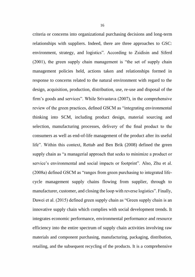
Hervani et al. (2005) discussed the processes that are involved in GSCM.

These processes are illustrated in Figure 2.2.

18

Figure 2.2: Process involved in green supply chain management (Hervani et al. 2005).

2.3.2 Importance of Green Supply Chain Management

Many studies examine the importance of green supply chain for companies

to improve their environmental and economic performance, compliance to

governments’ regulations, and help organization to achieve and sustain

competitive advantages.

Porter and van der Linde (1995) explained the fundamentals of greening as

a competitive initiative, since investment in greening could be profitable

through resource conserving, waste eliminating and productivity improving.

While, Kopicki et al. (1993) and Van Hoek (1999) suggested three

approaches in GSCM, reactive, proactive, and value seeking. In the reactive

approach, companies commit to minimal resources to environmental

19

management, by labeling product that are recyclable and use “pipe line

initiatives” to reduce the environmental impact of production. In the

proactive approach, commitment to new environmental initiative such as,

recycling of products and designing green products. In the value seeking

approach, companies integrate environmental activates into their strategies

such as green purchasing and ISO 14001 implementation.

The perspective of greening then change from the greening as a burden to

greening as a source of competitive advantage (Van Hoek, 1999). In a study

linking GSCM elements and performance measurement, Beamon (1999)

advocated for the traditional performance measurements systems structure

of supply chain must include mechanisms for product recovery. GSCM has

emerged as an important new archetype for companies to achieve profit and

market share objectives by lowering their environmental risks and impacts

and while raising their ecological efficiency (Van Hock, 1999) as mentioned

by (Zhu et al., 2005). While, Sinding (2000) emphasized that, the GSCM is

a necessary outcome of the evolution in environmental management from

“housekeeping” to product-related approaches (such as LCA), when a

company really wants to gain an environmental and competitive advantage.

Within this context, Kaiser et al. (2001) argued that, to address the

environmental issues proactively, it should consider all stages of product life

cycle during material selection and adopt purchasing mechanism to promote

the use of environmentally preferable products in the health care industry.

Zhu and Sarkis (2004) presented their empirical findings on the relationships

between GSCM practices and environmental and economic performance,

20

quality management, and Just-In-Time (JIT) or Lean manufacturing among

early adopters of green supply chain management practices in Chinese

manufacturing enterprises. They found that, the GSCM practices have Win-

Win relationships with environmental and economic performance, while

quality management has a positive moderator, so the organizations that

seriously consider the implementation of GSCM practices could benefit

greatly with introduction of Quality Management practices. Finally, the JIT

programs with internal environmental management practices may cause

further degradation of environmental performance, and care should be taken

when implementing GSCM programs in manufacturing organizations with

JIT philosophies in place. Theyel (2006) examined the importance of

collaboration between suppliers and customers as information exchange to

meet the environmental requirements. While, Testa and Iraldo (2010)

assessed the determinants and motivations for the implementation of green

supply chain management, and find that the company is able to involve its

business partners in the development of co-operative environmental plans,

the more it is able to achieve the expected results and improve its

performance. Wu and Pagell (2011) used theory building through case

studies to answer how do organizations balance short-term profitability and

long-term environmental sustainability when making supply chain decisions

under conditions of uncertainty. Zhu et al. (2012) focused on the importance

of coordinating internal and external GSCM practices to seek performance

improvements. Yang et al. (2013) studied the influence of internal green

practices and external green collaboration on the green performance and the

21

firm's competitiveness for container shipping industry. They found that, the

internal green practices and external green collaboration have positively

influence firm performance and competitiveness.

Then, the environmental and financial performance can be achieved by

implementing GSCM concepts in many sectors. Chiou et al. (2011)

demonstrated that many industrial sectors have improved their performance

through the implementation of GSCM concepts by greening the supplier,

which leads to green product innovation, green process innovation, and green

managerial innovation, as a results of this companies can acquire competitive

advantage.

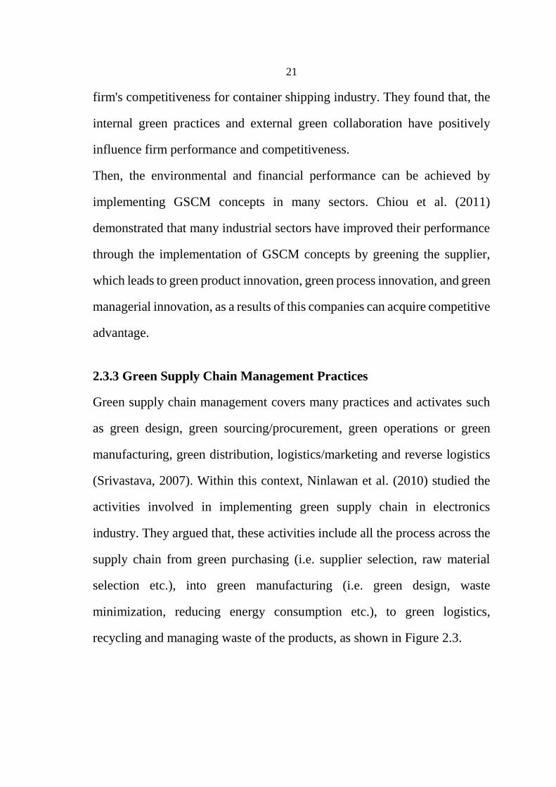
2.3.3 Green Supply Chain Management Practices

Green supply chain management covers many practices and activates such

as green design, green sourcing/procurement, green operations or green

manufacturing, green distribution, logistics/marketing and reverse logistics

(Srivastava, 2007). Within this context, Ninlawan et al. (2010) studied the

activities involved in implementing green supply chain in electronics

industry. They argued that, these activities include all the process across the

supply chain from green purchasing (i.e. supplier selection, raw material

selection etc.), into green manufacturing (i.e. green design, waste

minimization, reducing energy consumption etc.), to green logistics,

recycling and managing waste of the products, as shown in Figure 2.3.

22

Figure 2.3: Activities in Green Supply Chain (Ninlawan et al., 2010).

2.3.3.1 Green Design

The green design or eco-design is concerned with the development of

products that are more durable and energy-efficient; products that avoid the

use of toxic materials and can be easily disassembled for recycling (Gottberg

et al., 2006). These activities provide opportunities to minimize waste and

improve the efficiency of resource use through modifications in product size,

serviceable life and recyclability (Gottberg et al., 2006). On the other hand,

the green design may be presented a certain potential limitations or

disadvantages, which includes the following: the easily recyclable materials

may have substantial environmental impact during other life-cycle stages;

the obsolescence of the products in fashion-driven markets; the compatibility

23

with existing infrastructure and systems; the increased complexity; and the

increased risk of failure (Gottberg et al., 2006). The green design of product

could be used to analyze the product impact on environment during its life-

cycle (Life Cycle Assessment of the product). This approach is referred to as

a cradle-to-grave approach, which is a quantitative process for evaluating the

total environmental impact of a product over its life cycle (Mann et al, 1996).

2.3.3.2 Green Purchasing

Green purchasing is related to the increasingly heightened environmental

awareness, the decisions will impact through the purchase of materials that

are either recyclable or reusable or have already been recycled (Zhu et al.,

2008b; Sarkis, 2003). The importance of green purchasing for enterprises as

it pertains to the marketing of their products and the key elements of green

purchasing, which include: (1) the organizational framework, (2) a model for

supplier selection, (3) key factors and criteria affecting supplier selection and

(4) the establishment of beneficial buyer-supplier relationships (Zhu and

Geng, 2001). In this context, Min and Galle (2001) showed the effects of

green purchasing on suppliers selection, waste management, packaging, and

regulatory compliance.

2.3.3.3 Green Manufacturing

Manufacturing processes consume a lot of energy, chemicals and toxic

material that discharge a large amount of pollutants. Without effective

management, it can cause great damage to the environment. In a recent years,

green manufacturing has attracted a lot of attention, due to increasing

24

awareness of environment protection. Green manufacturing is a modern

manufacturing mode, it gives a comprehensive consideration of the

environment influence and resources efficiency, by minimizing the

environmental impact and maximizing the resources utilization (Li et al.,

2016). Melnyk and Smith (1996), as mentioned by Kannan et al. (2014),

defined green manufacturing as “a system that integrates product and process

design issues with issues of manufacturing planning and control in such a

manner to identify, quantify, assess, and manage the flow of environmental

waste with the goal of reducing and ultimately minimizing environmental

impact while trying to maximize resource efficiency”.

One of the main strategies of green manufacturing is the three R’s

(Remanufacture, Reduce, Reuse/Recycle), which includes policies such as

reducing hazardous waste volume, minimizing coolant consumption while

machining, and calculating a proper energy mix to ensure a sustainable

energy source (Dornfeld et al.,2013). Green manufacturing aims to reduce

the ecological burden by using appropriate materials and technologies, and

operations are intended to reduce, recycle, production planning and

scheduling, inventory management, remanufacturing, reuse, and product and

material recovery (Srivastava, 2007).

2.3.3.4 Waste Management

Human activities have always generated waste, poor management of these

wastes can lead to contamination of water, soil and atmosphere and to a

major impact on public health (Giusti, 2009).

25

Waste management makes it possible to know how well the processes are

designed for the prevention of waste. The management of waste passes

through several sources: reduction, pollution prevention and disposal, which

in turn include collection, transportation, incineration, composting, recycling

and disposal (Srivastava, 2007). Consequently, there will be a number of

system and process requirements that may change among the stages,

depending on the organization, industry and product type (Sarkis, 2003).

In general, all products have a life cycle cover a sequence of interrelated

activities from the acquisition of raw material until their end-of-life

management (Jofre and Morioka, 2005). There are five basic end of life

strategies that are classified according to their potential economic and

environmental efficiency to reuse, servicing, remanufacturing, recycling,

and disposal. Re-use represents the recovery and trade of used products or

their components as originally designed. Servicing is a strategy aimed at

extending the usage stage of a product by repair or maintenance.

Remanufacturing considers the process of removing specific parts of the

waste product for further re-use in new artifacts. Recycling (with or without

disassembly) includes the treatment, recovery, and reprocessing of materials

contained in used products or components in order to replace virgin materials

in the production of new goods. Finally, disposal entails the processes

incineration (with or without energy recovery) or landfill (Billatos, 1997;

Rose et al., 1999). The aim of all of these strategies is to maximize

profitability and efficiency (Jofre and Morioka, 2005).

26

2.3.3.5 Reverse Logistics

Reverse logistics focuses primarily on the return of recyclable or reusable

products and materials to the forward SC. The reverse logistics process has

identified a number of stages: collection, separation, densification,

transitional processing, delivery, and integration (Sarkis, 2003). Within this

context, Chouinard et al. (2005) dealt with problems related to the integration

of reverse logistics activities within a supply chain information system. They

defined reverse logistics as” the recovery and processing of unused products

and to the redistribution of reusable materials”. In fact, the integration of

reverse logistics within the regular supply chain aims to improve the

efficiency of the entire logistic network to meet the pressures exerted by the

environment (government agencies, competitors, customers, actors of the

supply chain). While, Srivastava and Srivastava (2006) presented a

framework to manage product returns for reverse logistics by focusing on

estimation of returns for selecting categories of products in the Indian

context. They developed a model that utilizes product ownership data,

average life cycle of products, post sales, forecasted demand and likely

impact of environmental policy measures for estimating return flows.

2.3.3.6 Green Logistics

Distribution and transportation operations form the important operational

characteristics in Logistics. These operations are more complicated when the

entire SC is considered. With the rapid increase of long-distance trade, SCs

are increasingly covering larger distances, consuming significantly more

27

fossil-fuel energy for transportation and emitting much more carbon dioxide

than they did a few decades ago (Venkat and Wakeland, 2006).

However, with increasing awareness about the effect of logistics activities

(i.e. transportation) on the global warming, air pollutions and energy usage

have been grown, which led to emerge of GL. There are several activities in

the field of GL such as redressing the distribution system, route optimization,

measuring the pollution levels, using alternative fuels and improving the

packaging design (Sharma, 2000). Furthermore, Martinsen and Huge-Brodin

(2010) summarized the GL innovations that can be adopted by companies

into nine categorizes as follows:

Vehicle technologies: the development in engine and exhaust systems,

aerodynamic profiling, reduction in vehicle tare weight and improved

tire performance can have an effect on environmental performance.

Alternative fuels: switching to a fuel with low carbon intensity such

as bio-fuel has implications for the environmental impact.

Mode choice and intermodal transports: carbon intensity of different

modes (road, rail, sea and air) varies and the proportion among them

also varies. Thus, it affects environmental impact. Intermodal

transports refer to a combination of different transport modes.

Behavioral aspects: eco-driving and defensive training are well known

measures to apply in order to lower environmental impact from

transports.

Logistics system design: this factor affects the distances that cargoes

are transported. It is used to minimize the total distance travelled by a

28

vehicle to deliver a certain amount of cargoes. Centralized versus

decentralized distribution structures is one parameter that can be of

importance for the environmental impact from logistics system.

Transport management: occupancy or fill rate and distances of empty

running vehicles are important aspects for environmental

performance. Route planning and orders aggregations or freight

consolidation are aspect of relevance.

Choice of partners: how to select the partners and how to manage the

relationships are two factors of interest when the aim is to lower the

environmental impact of supply chains.

2.4 Green Supply Chain Optimization

In this section, we will review the optimization models in Green Supply

Chain in strategic and tactical management levels (i.e. Network design) and

in tactical and operational management levels (i.e. Aggregate Production

Planning (APP)).

2.4.1 Green supply chain network optimization

The supply chain networks design is a strategic and tactical levels problem

aims to determine suppliers, facility location and transfer system

combinations or chains. “Supply chain network optimization refers to

models supporting strategic and tactical planning across the geographically

dispersed network of facilities operated by the company and those facilities

operated by the company's vendors and customers” (Shapiro, 2004) as

mentioned by (Tognetti et al., 2015).

29

Traditionally, the field of supply chain design has focused on economic

objectives, such as cost minimization and profit maximization, or on

performance-based objectives, including customer service level or supply

chain responsiveness (Liu and Papageorgiou, 2013; You and Grossmann,

2008). However, the advent of sustainability concerns have added several

new dimensions that are increasingly crucial in supply chain design and to

achieve truly sustainable solutions, a supply chain should be designed with

economic, environmental, and social sustainability criteria (Grossmann,

2004; Simões et al., 2014; Yue et al., 2014).

Many mathematical modeling was developed to address the problem of

network design in GSC. In this context, Bloemhof-Ruwaard et al., (1996)

used linear programming network flow to find optimal configurations and

reallocation of paper production, and the model used to analyze the scenarios

with different recycling strategies. This model consists of a mix of different

pulping technologies, a geographical distribution of pulp and paper

production, and a level of recycling consistent with the lowest environmental

impacts. While, Hugo and Pistikopoulos, (2005) developed a mathematical

programming-based methodology that integrated LCA criteria into the

design and planning decisions of supply chain networks. Multiple

environmental concerns were considered along with financial criteria in

formulating the planning task as an optimization problem. Strategic

decisions involving the selection, allocation and capacity expansion of

technologies along with the assignment of appropriate transportation modes

that would satisfy market demand were addressed using MIP. Neto et al. (2008)

30

introduced an integrated methodology of multi-objective programming that

balancing the environmental performance and process in design logistic

networks of European pulp and paper sector. While, Ramudhin et al. (2008)

tied greenhouse gases to carbon trading based on carbon market sensitive

green supply chain network design. They developed mixed integer

programing model (MIP) that focuses on the impact of transportation,

subcontracting, and production activities in terms of carbon footprint on the

design of a green supply chain network. The model integrates carbon prices

and exploits the opportunities offered by carbon market in the design of

green supply chain network. Tsai and Hung (2009) used fuzzy goal

programming approach to integrate activity-based costing (ABC) and

performance evaluation in a value chain structure for optimum selection of

suppliers and flow allocation in GSC, and the final objectives were

determined using Analytical Hierarchy Process (AHP) method that contains

the criteria of mission, circumstance, product stage, and precision degree. In

the same context, Diabat and Simchi-Levi (2009) introduced an optimization

model that integrates green supply chain network design problem with

carbon emission constraint using MIP. In their model, the throughput

capacity of the manufacturing site, storage capacity of the distribution

centers and their locations are considered as decision variables in order to

ensure that the total carbon emission does not exceed an emission cap while

minimizing the total supply chain cost. However, they found that as carbon

emission allowance decreases, supply chain total costs increase. Abdallah et

al. (2010) presented a different MIP in which the green procurement concept

31

where the decision on which supplier to choose affects the overall carbon

footprint of the supply chain is integrated in green supply chain network

design problem to minimize traditional supply chain cost in addition to

minimize the carbon emission cost.

Another related study is conducted by Paksoy et al. (2010), who considered

the green impact on a close-looped supply chain. A traditional network

design problem that minimizes the total transportation and purchasing costs

and tried to prevent more carbon emissions and encourage the customers to

use recyclable products was developed. They have presented different

transportation choices according to carbon emissions by using multi-

objective linear programming model. Sundarakani et al. (2010) developed an

analytical model that uses the long-range Lagrangian and the Eulerian

transport methods. The aim of this model is to minimize the CO2 emission

from both stationary and non-stationary across the supply chain processes,

by examining various heat transfer devices. This model helps to understand

the heat flux and carbon wastage at each node of the supply chain and allows

to calculate the total heat and carbon emission transferred from one stage of

the supply chain to another. While, Wang et al., (2011) were interested in the

environmental investment decision in the design of green supply chain

network and provided a multi-objective MIP model. The model linked the

decision of the environmental investment in the planning phase while its

environment influence in the operation phase. After conducting a sensitivity

analysis, the results showed that the total cost and CO2 emission would be

lower in supply chain networks with larger capacities. Pishvaee and Razmi,

32

(2012) proposed a multi-objective fuzzy optimization model for designing

both forward and reverse green supply chain under inherent uncertainty of

input data. The model aims to minimize the multiple environmental impact

by using LCA method, and to minimize the traditional cost to make balance

between them. To solve the problem, they developed an interactive fuzzy

solution approach. While, Elhedhli and Merrick (2012) developed a MIP

model alongside Lagrangian relaxation method, so that the relation between

carbon emission and vehicle weight is modeled to reduce the amount of

vehicle kilometers travelled and thereafter the combined costs of carbon

emission, fixed cost to set up facility, transportation and production costs can

be minimized. The results indicated that considering carbon emission cost

can change the optimal configuration of the network. Tognetti et al. (2015)

developed a multi-objective optimizations model for strategic production

networks planning that presents the interplay between emissions and the

costs of the supply chain contingent upon the production volume allocation

and the energy mix. The implementation of a practical case study in the

German automotive industry, shown that by optimizing the energy mix, the

CO2 emissions of the supply chain can be reduced by 30% at almost zero

variable cost increase. Talaei et al. (2015) proposed a novel bi-objective

facility location-allocation MILP model for CLGSC network design problem

that consisting of manufacturing/remanufacturing and collection/inspection

centers as well as disposal center and markets with uncertainties of the

variable costs and the demand rate. The aim of this model is to reduce the

network total costs and the rate of CO2 emission throughout the supply chain

33

network. The model has been developed using a robust fuzzy programming

approach to investigate the effects of uncertainties of the variable costs, as

well as the demand rate, on the network design. The ε-constraint approach

has been used to solve the bi-objective programming model. A numerical

study of Copiers Industry is used to show the applicability of the proposed

optimization model. Results have revealed that the model is capable of

controlling the network uncertainties as a result of which a robustness price

will be imposed on the system.

In context of relationship with suppliers and customers, Yeh and Chuang

(2011) developed an optimum mathematical planning model for green

partner selection, which involved four objectives such as minimization of the

total cost, minimization of the total time, maximization of the average

product quality and maximization of the green appraisal scores. They used

Multi-Objective Genetic Algorithms (MOGA) to find the set of Pareto-

optimal solutions. Kannan et al. (2013) proposed an integrated approach of

fuzzy multi attribute utility theory and multi-objective programming, for

rating and selecting the best green suppliers according to economic and

environmental criteria and then allocating the optimum order quantities

among them. The objective of the mathematical model is simultaneously to

maximize the total value of purchasing and to minimize the total cost of

purchasing. To handle the subjectivity of decision makers’ preferences,

fuzzy logic has been applied. The obtained results help organizations to

establish a systematic approach for tackling green supplier selection and

order allocation problems in a realistic situation. Within this context, Coskun

34

et al. (2016) proposed a Goal Programming (GP) model to measure the

relations between green supply chain network design and customer behavior,

to improve the practical efficiency of green supply chain networks, by

considering three customers segments according to their attitudes for green

products in the markets (i.e. green, inconsistent, and red customers), the

results have shown that the green supply chain network could be re-designed

cooperating with suppliers according to the expected greenness level of

suppliers and customers .

2.4.2 Aggregate production planning (APP) in GSC Optimization

One of the important subjects that could be addressed in tactical and

operational level of GSCM is Aggregate Production Planning (APP).

Chopra and Meindl (2013) defined aggregate planning as “a process by

which a company determines planned levels of capacity, production,

subcontracting, inventory, stockouts, and even pricing over a specified time

horizon”. While, Mirzapour et al. (2013) addressed APP as” an operational

activity that draws up an aggregate plan for the production process, in

advance of 3-18 months, to give an idea to management as to what quantity

of materials and other resources are to be produced and when, so that the

total cost of operations of the supply chain is kept minimum over that

period”. Also, Baykasoglu (2001) defined APP as “medium-term capacity

planning over 3–18 months planning horizon, which determines the optimum

production, workforce and inventory levels for each period of planning

horizon for a given set of production resources and constraints”.

35

By reviewing the literature relate to APP, there are numerous models that

have been developed with various degrees of complexity. In this context,

Hanssman and Hess (1960) developed a model on the LP approach using a

linear cost function of the decision variables. This model focused on

minimizing the total cost of regular payroll and over time, the cost of hiring

and firing, and the cost of holding inventory and shortages that incurred

during a given planning horizon. Haehling (1970) developed a multi-

product, and multi-stage production system model in which optimal

disaggregate decisions can be made under capacity constraints. Masud and

Hwang (1980) proposed three Multi Criteria Decision Making Methods

(MCDMs), its GP, sequential multi-objective and the step method. The three

methods are used to solve APP problems with minimizing cost, changes in

workforce levels, inventories, and backorders. In this context, Paiva and

Morabita (2009) developed a MIP model to support decisions in the APP of

sugar and ethanol milling companies. This model is based on the industrial

process selection and the production lot-sizing model. Sillekens et al. (2011)

proposed a MIP model for an APP problem of flow shop production lines in

automotive industry with special consideration of workforce consideration

flexibility. So their model, in contract to traditional approaches, considered

discrete capacity adaptions which originated from technical characteristics

of assembly lines, work regulations and shift planning. Ramezanian et al

(2012) developed a MILP model for general two-phase APP systems, with

consideration multi-period, multi-product and multi-machine systems with

setup decisions. The model was solved using genetic algorithm and Tabu

36

search methods. Mirzapour et al. (2011a) proposed a robust multi-objective

MINLP model for multi-site, multi-period, multi-product APP problem

under uncertainty in supply chain. The developed model considered two

conflicting objectives simultaneously, its cost parameters and demand

fluctuations under uncertainty.

With the increase of the environmental conscious and the globally trends to

reduce the effect of the supply chain and others industrials activities on the

human and environment, it becomes difficult to ignore the gap of

environmental aspects in the APP. In the context of green supply chain, by

reviewing the literature, the first attempt to integrate green concepts to APP,

was by Mirzapour et al. (2011b), by proposing a multi-period, multi-product

and multi-site APP in a GSCM by considering quantity discounts,

interrelationship between lead times and transportation cost, as well as lead

time and GHG emission, and backorders. While, Jamshidi et al. (2012)

proposed a multi-objective optimization model that considered the cost

elements of supply chain such as transportation, holding, and backorder cost

as well as the environmental aspects such as the amount of NO2, CO and the

volatile organic particles produced by facilities and transportation in the

supply chain. In this model, the facilities and transportation options have

capacity constraints. To solve the model, they utilized a new hybrid genetic

taguchi algorithm (GATA). Moreover, Mirzapour et al. (2013) developed a

more sophisticated model by proposing a stochastic programming approach

to solve a multi-period, multi-product, and multi-site aggregate production

planning in a green supply chain under the assumption of demand

37

uncertainty. This model considered flexible lead times, nonlinear purchase,

shortage cost functions and a GHG emission.

In the context of tactical planning, Fahimnia et al. (2015) developed a

multidimensional MINLP model for GSCM at tactical planning level. The

model aims to tradeoff between cost and environmental aspects including

carbon emissions, energy consumption and waste generation to investigate

the relationship between Lean practices (i.e. waste and lead time reduction)

and green outcomes. The Nested Integrated Cross-Entropy (NICE) method

has been developed to solve the proposed mixed-integer nonlinear

mathematical model. The applicability and the validity of the model are

investigated in an actual case problem, the results have shown that, not all

lean interventions at the tactical supply chain planning level result in green

benefits, and a flexible supply chain is the greenest and most efficient

alternative when compared to strictly lean and centralized situations.

Moreover, the model has shown how the organization can take advantage of

SC flexibility and agility through integrated lean and centralized situations

for more efficient environmental performance.

In the operational green supply chain planning level, Memari et al. (2015)

developed a novel multi-objective mathematical model in a green supply

chain network consisting of manufacturers, DCs and dealers in an

automotive manufacture case study. The aim of this model is to minimize

the total costs of production, distribution, holding and shortage cost at

dealers as well as minimizing environmental impact particularly the CO2

emission of supply chain network. This model can be used as a decision

38

support system in order determine the green economic production quantity

(GEPQ) using Just-In-Time (JIT) logistics. To solve the model, they used

MOGA in order to minimize the conflicting objectives simultaneously. The

performance of the proposed model is evaluated by calculating the gap

between the best results of the obtained Pareto fronts from MOGA and Goal

Attainment Programing (GAP) solver in Matlab.

2.5 Drivers’ Differences

2.5.1 The effect of drivers differences on fuel consumption

There are many factors affect fuel consumption and CO2 emission such as

driving behavior (i.e. gear changing), choice of travelling modes and route

choice etc. The holistic analysis of the factors that affect fuel consumption

and CO2 emission are shown in Figure 2.4.

Within this context, Ericsson (2001) investigated the effect of independent

driving patterns factors on emissions and fuel consumption. He used 16

independent driving patterns factors, by using different types of cars driven

by about 45 randomly chosen drivers. The results have shown that, by

applying regression analysis on the relation between driving pattern factor

and fuel-use and emissions, nine of driving pattern factors had an important

effect on fuel consumption and on emissions of HC, NOx, and CO2. Four of

the driving patterns factors describe different aspects of acceleration and

power demand, three factors describe aspects of gear-changing behavior and

two factors describe the effect of certain speed intervals/levels. The relation

between these nine driving patterns factors and fuel consumption and

39

emission as follow; factor for acceleration with strong power demand (+),

the stop factor (+), the speed oscillation factor (+), the factor of acceleration

with moderate power demand (+), the extreme acceleration factor (+), the

factor of speed 50-70 km/h (-), the factor of late gear changing from 2nd to

3rd gear (+), the factor for engine speed >3500 rpm (+) and the factor for

moderate engine speeds in 2nd and 3rd gear (-). This study shows that, these

independent driving patterns factors (i.e. acceleration and power demand,

gear changing behavior, and speed levels) are important explanatory

variables for emission and fuel consumption. He argued that, the needed to

focus on changing environments, drivers and vehicles in a way that does not

promote heavy acceleration, power demand and high engine speeds will be

a challenges for further research and development of traffic planning and

management, vehicle technology and driver education. Driver behavior is

one of the greatest factor determining the fuel consumption and CO2

emission of a heavy-duty vehicle and differences in fuel consumption can be

up to 30% depending on the driver (Nylund, 2006; Vangi and Virga, 2003).

Different drivers can obtain a different fuel consumption (and CO2 emission)

for the same car (Van der Voort et al., 2001). Within the context, Sivak and

Schoettle (2012), showed that the differences in drivers’ driving patterns can

lead to variation in fuel consumption and CO2 emission by more than 30%.

Also, Edmunds (2005) performed an argument that the moderate (normal)

driving yielded 31% better mileage than aggressive driving, on average.

40

Figure 2.4: Model describing factors that affect the amount of vehicular energy use and

exhaust emission (Ericsson, 2001).

There are many factors under the control of driver, if the driver avoids them,

45% reduction in fuel consumption and CO2 emission can be achieved such

as aggressive driving, excessive high speed, out of tune engine, neglect of

tire maintenance, air conditioning use, excessive idling, additional weight

and improper engine oils (Sivak and Schoettle, 2012). Alessandrini et al.

(2009) quantified the effect of some of parameters such as throttle standard

deviations and accelerator pedal on fuel consumption and CO2 emissions.

They argued that, the differences between drivers have a calm driving style

and aggressive one can result in differences in terms of fuel consumption

(and therefore CO2 emissions) up to 40%. Carrese et al. (2013) studied the

relationship between drivers’ behavior and fuel consumption and CO2

emission. They argued that, the differences in drivers’ behavior can lead

differences in fuel consumption and CO2 emission up to 27%. While, Tang

41

et al. (2015) developed an extended car-following to study the influences of

driver’s bounded rationally on his/ her micro driving behavior, and on fuel

consumption and gases emissions. The results have shown that considering

the driver’s bounded rationally will reduce his/her speed during the staring

process and improve the stability of the traffic flow during the evolution of

the small perturbation, and reduce fuel consumption and CO2 emission.

2.5.2 Eco-Driving

The road transportation is a major consumer of fossil fuel as well as a major

contributor to CO2 emission and then the environmental pollution. With

increase awareness about saving natural resources and protect the

environment as known as a sustainability. The need to reduce fuel

consumption and CO2 emission has been rapidly grown (Van der Voort et

al., 2001).

There are many methods for reducing fuel consumption and CO2 emission,

and these can be classified according to the horizon into long term and short

term methods. On the long term, the new technologies such as alternative

fuels, improving the rolling, air resistance, engine and transmission

efficiency of the vehicles, the potential savings by using this method is 49%

on average or by law and policy (i.e. setting goals and standards, and by

imposing taxes). On a short term, the factors that affect fuel consumption

include infrastructure changes (i.e. car pools lanes), traffic management

(because the congestion are closely related to fuel consumption and CO2

emission) with 5% fuel savings, and driver behavior, the changing in driver

42

behavior has a potential saving up to 15% (DeCicco and Ross, 1996).

Unwanted driving behaviors such as harsh acceleration, harsh breaking and

sudden steering are major for increased fuel consumption, air pollution (i.e.

GHG) and maintenance cost. Introduce driver to change his/her driving is

an effective way to reduce fuel consumption and CO2 emission in the short

term (Van der Voort et al., 2001). This lead to develop a new driving style

called Eco-Driving. Eco-driving is driving that is economical, ecological,

and safe, with the goal of reducing fuel consumption and greenhouse gas

emissions (Martin et al., 2012). Eco-driving practices have been found to be

effective in reducing energy consumption and CO2 emission, with potential

reduction reach to 20% (Barkenbus, 2010; Stillwater and Kurani, 2013).

With growing popularity of eco-driving courses as a powerful tool that can

improve drivers’ behavior in context of economic and ecologic performance,

numerous researches focus on the importance of Eco-driving behavior and

training as a strategic tool to reduce the fuel consumption and CO2 emission.

Barkenbus (2010) defined the characteristics of Eco-Driving such that

accelerating moderately, anticipating traffic flow and signals, avoiding

sudden starts and stops, driving within speed limit, and eliminating excessive

idling, etc. While, Sivak and Schoettle (2012) presented eco-driving in a

broadest way, Eco-Driving includes those strategic decisions (vehicles

selection and maintenance), tactical decisions (route selection and vehicle

load) and operational decisions (driver behavior) that improve vehicle fuel

economy and CO2 emission. In the strategic level, there are many factors

affect fuel consumption and CO2 emission such as; selection of vehicle class,

43

vehicle model, vehicle configuration; and vehicle maintenance (i.e. Tires’

pressure and engine oil), according to EPA (2011a), “fixing a car that is

noticeably out of tune or has failed an emission test can improve its gas

mileage by an average of 4%, through the results vary based on the kind of

repair and how well it is done”. Also, “fixing a faulty oxygen sensor can

improve mileage by as much as 40%” (EPA, 2011b). At tactical level, the

driver in this level is responsible for selecting the best routes based on road

type, grade and congestion. First, different road types result in difference in

fuel consumption and CO2 emission, because the average speeds, profiles of

acceleration and deceleration depend on the road type. A recent Canadian

study (Natural Resources Canada, 2009) found that a highways with average

speed of 80 km/h is better than other roads with about 9%. The second

responsibility of the driver is selecting the most flat route among the

available alternatives. Boriboonsomsin and Barth (2009) found that the fuel

consumption has nonlinear relationship with the road grade in a particular

scenario with the same origin and destination but two alternative routes, a

longer but flat route yielded 15-20% better fuel economy and CO2 emission

than a shorter hilly route. Third, the ability of driver to avoid the more

congested routes can save fuel consumption and reduce CO2 emission by 10-

20%. TRB (2000) classified the road according to the level of services (i.e.

congestion) into six categories: A (free flow), B (reasonably free flow), C

(stable flow), D (approaching unstable flow), E (unstable flow) and F (forced

or breakdown flow). Facanha (2009) used these categories and indicated that

depending on the vehicle type and road type the reduction in fuel

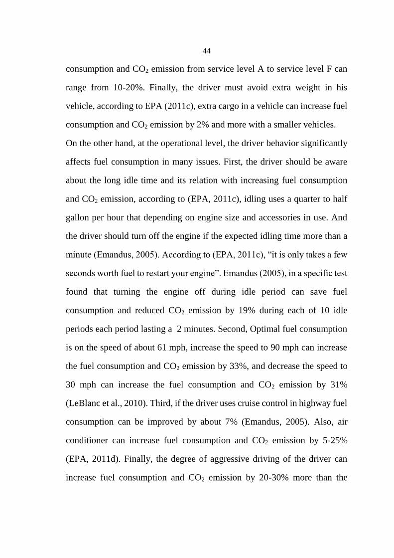
44

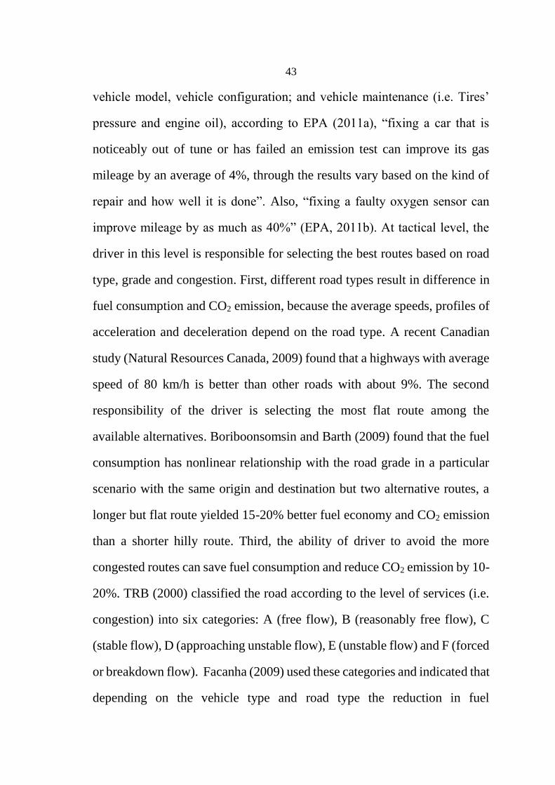
consumption and CO2 emission from service level A to service level F can

range from 10-20%. Finally, the driver must avoid extra weight in his

vehicle, according to EPA (2011c), extra cargo in a vehicle can increase fuel

consumption and CO2 emission by 2% and more with a smaller vehicles.

On the other hand, at the operational level, the driver behavior significantly

affects fuel consumption in many issues. First, the driver should be aware

about the long idle time and its relation with increasing fuel consumption

and CO2 emission, according to (EPA, 2011c), idling uses a quarter to half

gallon per hour that depending on engine size and accessories in use. And

the driver should turn off the engine if the expected idling time more than a

minute (Emandus, 2005). According to (EPA, 2011c), “it is only takes a few

seconds worth fuel to restart your engine”. Emandus (2005), in a specific test

found that turning the engine off during idle period can save fuel

consumption and reduced CO2 emission by 19% during each of 10 idle

periods each period lasting a 2 minutes. Second, Optimal fuel consumption

is on the speed of about 61 mph, increase the speed to 90 mph can increase

the fuel consumption and CO2 emission by 33%, and decrease the speed to

30 mph can increase the fuel consumption and CO2 emission by 31%

(LeBlanc et al., 2010). Third, if the driver uses cruise control in highway fuel

consumption can be improved by about 7% (Emandus, 2005). Also, air

conditioner can increase fuel consumption and CO2 emission by 5-25%

(EPA, 2011d). Finally, the degree of aggressive driving of the driver can

increase fuel consumption and CO2 emission by 20-30% more than the

45

moderate driving (LeBlanc et al., 2010; Emandus, 2005). These decisions

and their effect on fuel consumption and CO2 emission are shown in Table 2.1.

Table 2.1: The effect of driver on fuel consumption and CO2 emission at

different levels (Sivak and Schoettle, 2012).

Within this context, Kurani et al. (2015) identified six categories for Eco-

Driving behavior by reviewing the popular and academic sources of Eco-

Driving. The six categories and their characteristics are shown in Table 2.2.

46

Table 2.2: Categories of Eco-Driving behavior and some of their

psychologically attributes (Kurani et al., 2015).

Barkenbus (2010) argued that, the characteristics of Eco-driving involve

such thing as accelerating moderately (with shift ups between 2000 and 2500

revolutions for those with manual transmissions); anticipating traffic flow

and signals, thereby avoiding sudden starts and stops; maintaining an even

driving pace (using cruise control on the highway where appropriate);

driving at or safely below the speed limit; eliminating excessive idling;

maintaining optimum tire pressure and the regular changing of air filters,

with advantages are reduce CO2 emission, cost of driving, and producing

tangible and well know safely benefits (with fewer accidents and traffic

fatalities).

47

Within this context, numerous previous studies emphasized that the Eco-

driving behavior of the driver can reduce fuel consumption and CO2 emission

up to 10%, and with motivating drivers by providing incentive system, the

eco-driving behavior can reduce fuel consumption and CO2 emission up to

25% (Barkenbus, 2010; Vagg et al, 2013). Also, Alam and McNabola (2014)

in a comprehensive review of driving behavior, showed that the

improvement in fuel economy can reach to 45% by adopting eco-driving

strategies. Training, monitoring, and feedback are ways of guiding drivers

towards more fuel efficient driving patterns. Liimatainen (2011) developed

a methodology for fairly measuring drivers’ performance that helps

organizations to apply incentive system that motivates drivers to achieve its

energy efficiency targets.

2.6 Green Human Resources Management (GHRM) in Supply Chain

Management (SCM)

Green Human Resources Management (GHRM) and Green Supply Chain

Management (GSCM) are popular subjects in the areas of Human Resources

Management (HRM) and Operations Management (OM), respectively.

Human resources practices are critical for implementation and maintenance

of environmental management systems (Jabbour and Santos, 2008; Daily et

al., 2011). Human aspects are fundamental to adoption of advanced

environmental practices (Sarkis et al., 2010; Graves et al., 2013).

Environmental training stands out as one of the primary methods through

48

which human resources support environmental management (Daily et al.,

2012; Jabbour et al., 2013).

Within this context, Daily and Hung (2001) stated that each of the phases of

an environmental management system required the specific support of a

human resources practice, with emphasis on recruitment and selection,

training, performance evaluation, and rewards for employees. In the context

of GSCM, Jabbour and de Sousa Jabbour (2015) constructed a framework

that integrated GHRM and GSCM. They argued that, the GHRM practices

such as recruitment and selection, training, performance evaluation,

empowerment, and rewards are important to implementing GSCM. Also, the

truly implementation of GSCM cannot be archived without integration of

these paradigms.

With increasing awareness about the effect of drivers’ on fuel consumption

and CO2 emission and the differences between them depending on their

driving patterns, experience in route selection, maintenance issues,

awareness about environmental issues, motivation to adopt a green initiatives

and to improve their performance, and the training they own. This leads to

increase importance of human resource practices in selection drivers, testing,

training and motivating them, assigning them to the appropriate vehicles and

destinations, monitoring them, evaluating their performance, and rewarding

them based on the fairly incentive system. In such way that, implementing

GSCM for reducing CO2 emission across the supply chain could be truly

achieved.

49

2.8 Summary

This chapter introduced the readers to sufficient knowledge about the supply

chain and their planning scope, green supply chain management, their

practices and the importance of GSCM to improve the firms’ environmental

and economic performance. This chapter presents many optimization models

in green supply chain management that aim to minimize the environmental

effect of supply chain (i.e.CO2 emission) as well as minimizing the total cost.

And then, the significance of driver behavior as a factor that influences fuel

consumption and CO2 emission and the importance of Eco-driving as a tool

that helps organization to manage their drivers’ behavior to improve their

environmental and economic performance in their supply chains networks

have been presented. Finally, the importance of GHRM in implementing and

adopting GSCM and focusing on the drivers as an important human source

should be taken into account in managing and designing GSCM to minimize

the CO2 emission and fuel consumption.

50

Chapter Three

Model Formulation

51

Chapter Three

Model Formulation

3.1 Overview

This chapter presents the mathematical formulation of the proposed model.

The proposed model was developed as a Mixed Integer Non Linear

Programming (MINLP) Model and then converted to a linear one. At first,

this chapter presents to the reader the basic concepts of MINLP/MILP model.

And then, the model description will be introduced, that includes the model’s

assumptions, sets, parameters, decision variables, objective function

components and constraints.

3.2 Mixed Integer Non Linear Programming (MINLP)

Linear Programming (LP) is the problem of optimizing (minimizing or

maximizing) a linear function subject to a linear constraints. A wide variety

of practical problems, from nutrition, transportation, production planning,

finance, and many more areas can be modeled as linear programming. All

decision variables in the LP have been continuous, in the sense that decision

variables are allowed to be fractional. At some scenarios, the fractional

solutions are not realistic. Which led to develop another optimization

problem, such as the following:

Objective Function:

Maximize or Minimize ∑ 𝐶𝑗𝑥𝑗𝑛𝑗=1

Subject to:

52

∑ 𝑎𝑖𝑗𝑥𝑗 = 𝑏𝑖 (𝑖 = 1,2, … , 𝑚)𝑛

𝑗=1,

𝑥𝑗 ≥ 0 (𝑗 = 1,2, … , 𝑛),

𝑥𝑗 𝑖𝑛𝑡𝑒𝑔𝑒𝑟 (𝑓𝑜𝑟 𝑠𝑜𝑚𝑒 𝑜𝑟 𝑎𝑙𝑙 𝑗 = 1,2, … , 𝑛)

This is called Integer Programming (IP) problem. It is said to be a Mixed

Integer Linear Program (MILP) when some, but not all, variables are

restricted to be integer (discrete variables), and is called pure integer program

when all decision variables must be integers, and in the two previous cases

the objective function and all the constraints must be linear.

Many optimal decision problems in scientific, engineering, and public sector

applications involve both discrete decisions and nonlinear system dynamics

that affect the quality of the final design or plan. Mixed-integer nonlinear

programming (MINLP) problems combine the combinatorial difficulty of

optimizing over discrete variable sets with the challenges of handling

nonlinear functions. MINLP is one of the most general modeling paradigms

in optimization and includes both nonlinear programming (NLP) and mixed-

integer linear programming (MILP) as sub-problems. Mixed Integer

Nonlinear Programming (MINLP) refers to mathematical programming with

continuous and discrete variables and nonlinearities in the objective function

and constraints. The use of MINLP is a natural approach of formulating

problems where it is necessary to simultaneously optimize the system

structure (discrete) and parameters (continuous). MINLP has been used in

various applications, including the process industry and the financial,

engineering, management science and operations research sectors. It

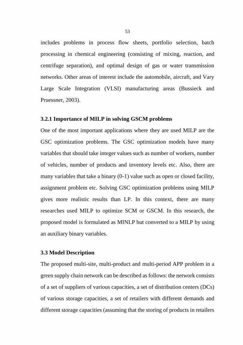
53

includes problems in process flow sheets, portfolio selection, batch

processing in chemical engineering (consisting of mixing, reaction, and

centrifuge separation), and optimal design of gas or water transmission

networks. Other areas of interest include the automobile, aircraft, and Vary

Large Scale Integration (VLSI) manufacturing areas (Bussieck and

Pruessner, 2003).

3.2.1 Importance of MILP in solving GSCM problems

One of the most important applications where they are used MILP are the

GSC optimization problems. The GSC optimization models have many

variables that should take integer values such as number of workers, number

of vehicles, number of products and inventory levels etc. Also, there are

many variables that take a binary (0-1) value such as open or closed facility,

assignment problem etc. Solving GSC optimization problems using MILP

gives more realistic results than LP. In this context, there are many

researches used MILP to optimize SCM or GSCM. In this research, the

proposed model is formulated as MINLP but converted to a MILP by using

an auxiliary binary variables.

3.3 Model Description

The proposed multi-site, multi-product and multi-period APP problem in a

green supply chain network can be described as follows: the network consists

of a set of suppliers of various capacities, a set of distribution centers (DCs)

of various storage capacities, a set of retailers with different demands and

different storage capacities (assuming that the storing of products in retailers

54

is possible), as all suppliers, DCs and retailers spread geographically; the

distance from suppliers to DCs and from DCs to retailers can differ, (as

shown in Figure 3.1). Also, there are a set of products types, a set of vehicle

types, each vehicle type has an amount of fuel consumption and

𝐶𝑂2 emissions per unit distance, and finally there are a set of drivers, who

are classified into three levels according to their green driving indices (𝐺𝐷𝐼),

each level of 𝐺𝐷𝐼 for drivers has different effects based on the fuel

consumption and 𝐶𝑂2 emissions. Green Driving Index (𝐺𝐷𝐼) is an index

used to measure the driver’s readiness according to environmental issues,

and there are some factors that might be used in evaluating the driver’s

readiness such as awareness about green issues, experience about

transportation networks. Sivak and Schoettle (2012) showed that, the

decisions that drivers take such as strategic decision (i.e. maintenance issue),

tactical decision (i.e. route selection) and operational decision (i.e. driving

behavior), affect vehicles fuel consumption (and therefore 𝐶𝑂2emission).

Also, driving patterns (i.e. sportive, aggressive, or Eco-driving patterns)

adopted by drivers affecting on the degree to which extent the driver has a

green driving index (𝐺𝐷𝐼). Alessandrini et al. (2009), argued that the driver’s

driving style can lead to different in fuel consumption and 𝐶𝑂2 emission up

to 40% in comparison between a calm driver and an aggressive one. In this

thesis, we assume that the three levels of drivers are different according to

their driving patterns (styles), the driver of level one has an aggressive

driving pattern, the driver of level two has a calm or moderate driving pattern

and the driver of level three has an Eco-driving patterns. Furthermore, the

55

motives s/he has owned either materialistic or non-materialistic can

influence on the driver’s style and to which extent the driver adopt eco-

driving behavior. Lai (2015) emphasized that providing incentive system to

motivate drivers to adopt Eco-driving, will lead to improve their economic

and environmental performance, and therefore improve their 𝐺𝐷𝐼𝑠. So, high

𝐺𝐷𝐼𝑠 can be reinforced and achieved by applying training courses and

reward incentive system, to encourage drivers to keep their 𝐺𝐷𝐼𝑠 high and

adopting Eco-driving style. As mentioned in the previous studies, the

suitable driver training and using monetary reward system can reduce fuel

consumption and 𝐶𝑂2emission by 10% on average (Young et al, 2011;

Zarkadoula et al, 2007). So the environmental and economic performance

will be improved across the entire supply chain network. The proposed

model is to minimize the total costs and 𝐶𝑂2 emission in the entire supply

chain and fulfill the various demands at the retailers, so the problem is to

determine: (1) which products to ship from suppliers to DCs and from DCs

to retailers in each period, (2) the quantity of products should be stored at

each DC and each retailer in each period, (3) the number of vehicles from

each vehicle types should be used to transport products from each

distribution center to each retailer in each period, (4) the optimal assignment

among vehicles and drivers by taking into account the vehicle types and the

green driving index (GDI) of the drivers, so each driver's assign to one and

only one vehicle and vice versa, and then assigned these pairs of vehicles

and drivers to each shipments of products from DCs to retailers according

to distances between DCs and retailers, so the model should select the

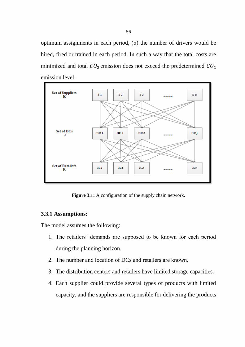
56

optimum assignments in each period, (5) the number of drivers would be

hired, fired or trained in each period. In such a way that the total costs are

minimized and total 𝐶𝑂2 emission does not exceed the predetermined 𝐶𝑂2

emission level.

Figure 3.1: A configuration of the supply chain network.

3.3.1 Assumptions:

The model assumes the following:

1. The retailers’ demands are supposed to be known for each period

during the planning horizon.

2. The number and location of DCs and retailers are known.

3. The distribution centers and retailers have limited storage capacities.

4. Each supplier could provide several types of products with limited

capacity, and the suppliers are responsible for delivering the products

57

to each distribution center, so the purchasing cost includes the product

cost, transportation cost and ordering cost.

5. The lead time to ship products from DCs to retailers is assumed to be

zero, so it is ignored.

6. The vehicles are being rented from a third party, and the fixed costs

associated with the rental of vehicles paid each period, and vary

depending on the type of vehicles.

7. There are three types of vehicles that vary in their cost (i.e. rental and

variable costs), capacity, and the amount of CO2 that will be emitted.

8. There are three levels of drivers who are classified depending on their

driving patterns. Driver level 1 has an aggressive driving pattern,

driver level 2 has a moderate/calm driving pattern, and driver level 3

has an eco-driving pattern. As the level of driver increases, his/her

efficiency in reducing fuel consumption and CO2 emission will

increase. In such a way that, the difference between each level in term

of fuel consumption and CO2 emission is 20% (Barkenbus, 2010;

Stillwater and Kurani, 2013).

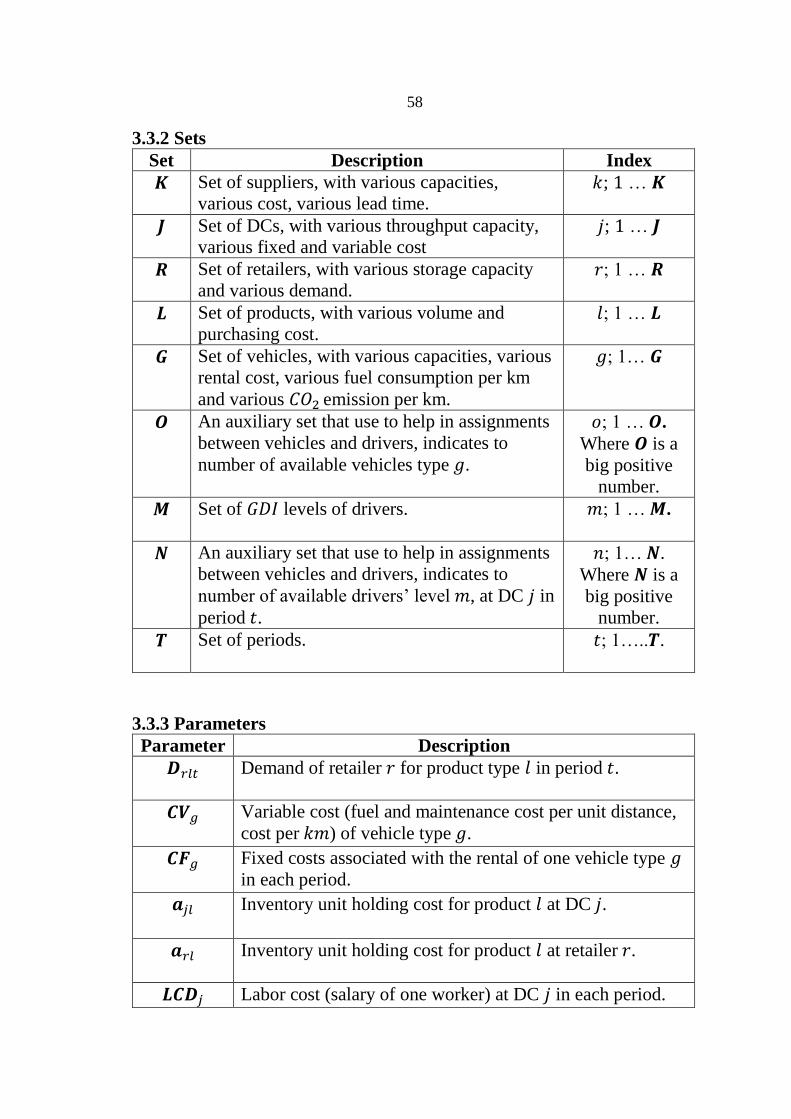
58

3.3.2 Sets

Set Description Index

𝑲 Set of suppliers, with various capacities,

various cost, various lead time. 𝑘; 1 … 𝑲

𝑱 Set of DCs, with various throughput capacity,

various fixed and variable cost 𝑗; 1 … 𝑱

𝑹 Set of retailers, with various storage capacity

and various demand. 𝑟; 1 … 𝑹

𝑳 Set of products, with various volume and

purchasing cost. 𝑙; 1 … 𝑳

𝑮

Set of vehicles, with various capacities, various

rental cost, various fuel consumption per km

and various 𝐶𝑂2 emission per km.

𝑔; 1… 𝑮

𝑶 An auxiliary set that use to help in assignments

between vehicles and drivers, indicates to

number of available vehicles type 𝑔.

𝑜; 1 … 𝑶.

Where 𝑶 is a

big positive

number.

𝑴

Set of 𝐺𝐷𝐼 levels of drivers. 𝑚; 1 … 𝑴.

𝑵

An auxiliary set that use to help in assignments

between vehicles and drivers, indicates to

number of available drivers’ level 𝑚, at DC 𝑗 in

period 𝑡.

𝑛; 1… 𝑵.

Where 𝑵 is a

big positive

number.

𝑻

Set of periods. 𝑡; 1…..𝑻.

3.3.3 Parameters

Parameter Description

𝑫𝑟𝑙𝑡

Demand of retailer 𝑟 for product type 𝑙 in period 𝑡.

𝑪𝑽𝑔

Variable cost (fuel and maintenance cost per unit distance,

cost per 𝑘𝑚) of vehicle type 𝑔.

𝑪𝑭𝑔

Fixed costs associated with the rental of one vehicle type 𝑔

in each period.

𝒂𝑗𝑙

Inventory unit holding cost for product 𝑙 at DC 𝑗.

𝒂𝑟𝑙

Inventory unit holding cost for product 𝑙 at retailer 𝑟.

𝑳𝑪𝑫𝑗 Labor cost (salary of one worker) at DC 𝑗 in each period.

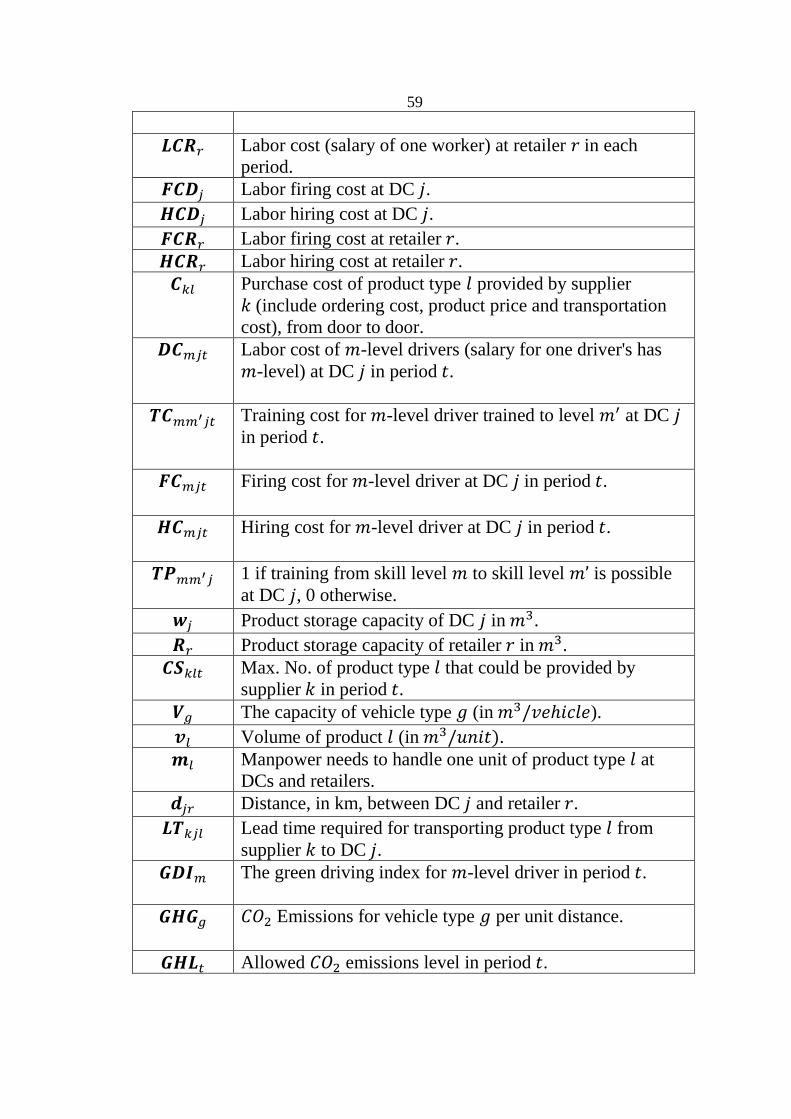
59

𝑳𝑪𝑹𝑟 Labor cost (salary of one worker) at retailer 𝑟 in each

period.

𝑭𝑪𝑫𝑗 Labor firing cost at DC 𝑗.

𝑯𝑪𝑫𝑗 Labor hiring cost at DC 𝑗.

𝑭𝑪𝑹𝑟 Labor firing cost at retailer 𝑟.

𝑯𝑪𝑹𝑟 Labor hiring cost at retailer 𝑟.

𝑪𝑘𝑙

Purchase cost of product type 𝑙 provided by supplier

𝑘 (include ordering cost, product price and transportation

cost), from door to door.

𝑫𝑪𝑚𝑗𝑡 Labor cost of 𝑚-level drivers (salary for one driver's has

𝑚-level) at DC 𝑗 in period 𝑡.

𝑻𝑪𝑚𝑚′𝑗𝑡 Training cost for 𝑚-level driver trained to level 𝑚′ at DC 𝑗

in period 𝑡.

𝑭𝑪𝑚𝑗𝑡

Firing cost for 𝑚-level driver at DC 𝑗 in period 𝑡.

𝑯𝑪𝑚𝑗𝑡

Hiring cost for 𝑚-level driver at DC 𝑗 in period 𝑡.

𝑻𝑷𝑚𝑚′𝑗

1 if training from skill level 𝑚 to skill level 𝑚’ is possible

at DC 𝑗, 0 otherwise.

𝒘𝑗 Product storage capacity of DC 𝑗 in 𝑚3.

𝑹𝑟 Product storage capacity of retailer 𝑟 in 𝑚3.

𝑪𝑺𝑘𝑙𝑡 Max. No. of product type 𝑙 that could be provided by

supplier 𝑘 in period 𝑡.

𝑽𝑔 The capacity of vehicle type 𝑔 (in 𝑚3/𝑣𝑒ℎ𝑖𝑐𝑙𝑒).

𝒗𝑙 Volume of product 𝑙 (in 𝑚3/𝑢𝑛𝑖𝑡).

𝒎𝑙 Manpower needs to handle one unit of product type 𝑙 at

DCs and retailers.

𝒅𝑗𝑟 Distance, in km, between DC 𝑗 and retailer 𝑟.

𝑳𝑻𝑘𝑗𝑙 Lead time required for transporting product type 𝑙 from

supplier 𝑘 to DC 𝑗.

𝑮𝑫𝑰𝑚

The green driving index for 𝑚-level driver in period 𝑡.

𝑮𝑯𝑮𝑔

𝐶𝑂2 Emissions for vehicle type 𝑔 per unit distance.

𝑮𝑯𝑳𝑡 Allowed 𝐶𝑂2 emissions level in period 𝑡.

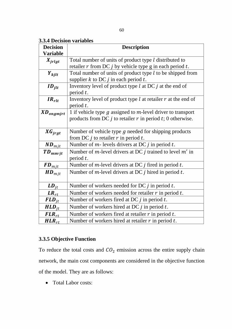
60

3.3.4 Decision variables

Decision

Variable

Description

𝑿𝒋𝒓𝒍𝒈𝒕 Total number of units of product type 𝑙 distributed to

retailer 𝑟 from DC 𝑗 by vehicle type g in each period 𝑡.

𝒀𝒌𝒋𝒍𝒕 Total number of units of product type 𝑙 to be shipped from

supplier 𝑘 to DC 𝑗 in each period 𝑡.

𝑰𝑫𝒋𝒍𝒕 Inventory level of product type 𝑙 at DC 𝑗 at the end of

period 𝑡.

𝑰𝑹𝒓𝒍𝒕 Inventory level of product type 𝑙 at retailer 𝑟 at the end of

period 𝑡.

𝑿𝑫𝒐𝒏𝒈𝒎𝒋𝒓𝒕 1 if vehicle type 𝑔 assigned to 𝑚-level driver to transport

products from DC 𝑗 to retailer 𝑟 in period 𝑡; 0 otherwise.

𝑿𝑮𝒋𝒓𝒈𝒕 Number of vehicle type 𝑔 needed for shipping products

from DC 𝑗 to retailer 𝑟 in period 𝑡.

𝑵𝑫𝑚𝑗𝑡 Number of 𝑚- levels drivers at DC 𝑗 in period 𝑡.

𝑻𝑫𝒎𝒎′𝒋𝒕 Number of 𝑚-level drivers at DC 𝑗 trained to level 𝑚′ in

period 𝑡.

𝑭𝑫𝑚𝑗𝑡 Number of 𝑚-level drivers at DC 𝑗 fired in period 𝑡.

𝑯𝑫𝑚𝑗𝑡

Number of 𝑚-level drivers at DC 𝑗 hired in period 𝑡.

𝑳𝑫𝑗𝑡 Number of workers needed for DC 𝑗 in period 𝑡.

𝑳𝑹𝑟𝑡 Number of workers needed for retailer 𝑟 in period 𝑡.

𝑭𝑳𝑫𝑗𝑡 Number of workers fired at DC 𝑗 in period 𝑡.

𝑯𝑳𝑫𝑗𝑡 Number of workers hired at DC 𝑗 in period 𝑡.

𝑭𝑳𝑹𝑟𝑡 Number of workers fired at retailer 𝑟 in period 𝑡.

𝑯𝑳𝑹𝑟𝑡 Number of workers hired at retailer 𝑟 in period 𝑡.

3.3.5 Objective Function

To reduce the total costs and 𝐶𝑂2 emission across the entire supply chain

network, the main cost components are considered in the objective function

of the model. They are as follows:

Total Labor costs:

61

∑ 𝐿𝐶𝐷𝑗𝑗,𝑡 × 𝐿𝐷𝑗𝑡+∑ 𝐿𝐶𝑅𝑟𝑟,𝑡 × 𝐿𝑅𝑟𝑡+∑ 𝐹𝐶𝐷𝑗𝑗,𝑡 ×

𝐹𝐿𝐷𝑗𝑡 + ∑ 𝐻𝐶𝐷𝑗𝑗,𝑡 × 𝐻𝐿𝐷𝑗𝑡 + ∑ 𝐹𝐶𝑅𝑟𝑟,𝑡 × 𝐹𝐿𝑅𝑟𝑡 +

∑ 𝐻𝐶𝑅𝑟𝑟,𝑡 × 𝐻𝐿𝑅𝑟𝑡 + ∑ 𝐷𝐶𝑚𝑗𝑡 × 𝑁𝐷𝑚𝑗𝑡 +𝑗,𝑚,𝑡

∑ 𝐹𝐶𝑚𝑗𝑡 × 𝐹𝐷𝑚𝑗𝑡 + ∑ 𝐻𝐶𝑚𝑗𝑡 × 𝐻𝐷𝑚𝑗𝑡𝑚,𝑗,𝑡𝑗,𝑚,𝑡 +

∑ 𝑇𝐶𝑚𝑚′𝑗𝑡𝑚,𝑚′,𝑗,𝑡 × 𝑇𝐷𝑚𝑚′𝑗𝑡

(1)

Description of equation (1): summation of labor cost (salary of one

worker) at DC 𝑗 × number of workers needed for DC 𝑗 in period 𝑡 +

Summation of labor cost (salary of one worker) at retailer 𝑟 in each

period × number of workers needed for retailer 𝑟 in period 𝑡+

Summation of labor firing cost at DC 𝑗 × number of workers fired at

DC 𝑗 in period 𝑡+ summation of labor hiring cost at DC 𝑗 × number

of workers hired at DC 𝑗 in period 𝑡+ summation of labor firing cost

at retailer 𝑟 × number of workers fired at retailer 𝑟 in period 𝑡+

Summation of labor hiring cost at retailer 𝑟 × number of workers

hired at retailer 𝑟 in period 𝑡+ summation of labor cost of 𝑚-level

drivers (salary for one driver's has 𝑚-level) at DC 𝑗 in period 𝑡 ×

number of 𝑚- levels drivers at DC 𝑗 in period 𝑡+summation of firing

cost for 𝑚-level driver at DC 𝑗 in period 𝑡 × number of 𝑚-level

drivers at DC 𝑗 fired in period 𝑡+ summation of hiring cost for 𝑚-

level driver at DC 𝑗 in period 𝑡 × number of 𝑚-level drivers at DC 𝑗

hired in period 𝑡+summation of training cost for 𝑚-level driver

trained to level 𝑚′ at DC 𝑗 in period 𝑡 × number of 𝑚-level drivers

at DC 𝑗 trained to level 𝑚′ in period 𝑡.

62

Total Inventory cost:

∑ 𝑎𝑗𝑙𝑗,𝑙,𝑡 × 𝐼𝐷𝑗𝑙𝑡 + ∑ 𝑎𝑟𝑙𝑟,𝑙,𝑡 × 𝐼𝑅𝑟𝑙𝑡 (2)

Description of equation (2): summation of inventory unit holding

cost for product 𝑙 at DC 𝑗 × inventory level of product type 𝑙 at DC 𝑗

at the end of period 𝑡+summation of inventory unit holding cost for

product 𝑙 at retailer 𝑟 × inventory level of product type 𝑙 at

retailer 𝑟 at the end of period 𝑡.

Total Transportation cost that includes fixed and variable costs, the

fixed cost depends on the number of vehicles needed of each type in

each period, and the variable cost depends on the types of vehicles

used and the drivers assigned to these vehicles as well as on the

distances between distribution centers and retailers. The drivers have

an inverse effect on the fuel consumption (variable cost) depending on

their 𝐺𝐷𝐼. As the 𝐺𝐷𝐼 of the driver increases the fuel consumption as

well as the variable cost decreases:

∑ 𝐶𝐹𝑔𝑗,𝑟,𝑔,𝑡 × 𝑋𝐺𝑗𝑟𝑔𝑡 + ∑ 𝐶𝑉𝑔𝑗,𝑟,𝑔,𝑜,𝑚,𝑛,𝑡 × 𝑑𝑗𝑟 ×1

𝐺𝐷𝐼𝑚 ×

𝑋𝐷𝑗𝑟𝑔𝑜𝑚𝑛𝑡 (3)

Explanation of equation (3): summation of fixed costs associated

with the rental of one vehicle type 𝑔 in each period × number of

vehicle type 𝑔 needed for shipping products from DC 𝑗 to retailer 𝑟

in period 𝑡 +summation of variable cost (fuel and maintenance cost

per unit distance, cost per 𝑘𝑚) of vehicle type 𝑔 × distance, in km,

between DC 𝑗 and retailer 𝑟 ×(1/ green driving index for 𝑚-level

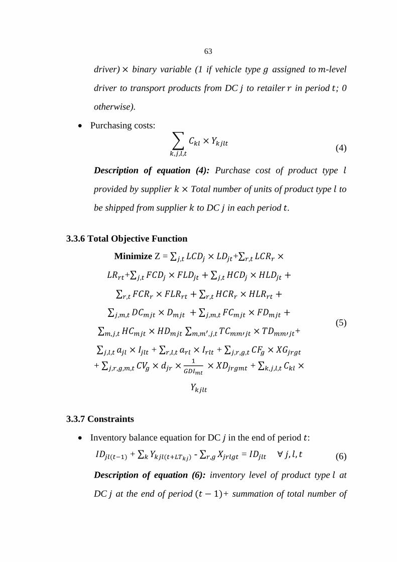
63

driver) × binary variable (1 if vehicle type 𝑔 assigned to 𝑚-level

driver to transport products from DC 𝑗 to retailer 𝑟 in period 𝑡; 0

otherwise).

Purchasing costs:

∑ 𝐶𝑘𝑙

𝑘,𝑗,𝑙,𝑡

× 𝑌𝑘𝑗𝑙𝑡 (4)

Description of equation (4): Purchase cost of product type 𝑙

provided by supplier 𝑘 × Total number of units of product type 𝑙 to

be shipped from supplier 𝑘 to DC 𝑗 in each period 𝑡.

3.3.6 Total Objective Function

Minimize Z = ∑ 𝐿𝐶𝐷𝑗𝑗,𝑡 × 𝐿𝐷𝑗𝑡+∑ 𝐿𝐶𝑅𝑟𝑟,𝑡 ×

𝐿𝑅𝑟𝑡+∑ 𝐹𝐶𝐷𝑗𝑗,𝑡 × 𝐹𝐿𝐷𝑗𝑡 + ∑ 𝐻𝐶𝐷𝑗𝑗,𝑡 × 𝐻𝐿𝐷𝑗𝑡 +

∑ 𝐹𝐶𝑅𝑟𝑟,𝑡 × 𝐹𝐿𝑅𝑟𝑡 + ∑ 𝐻𝐶𝑅𝑟𝑟,𝑡 × 𝐻𝐿𝑅𝑟𝑡 +

∑ 𝐷𝐶𝑚𝑗𝑡 × 𝐷𝑚𝑗𝑡 + ∑ 𝐹𝐶𝑚𝑗𝑡 × 𝐹𝐷𝑚𝑗𝑡 +𝑗,𝑚,𝑡𝑗,𝑚,𝑡

∑ 𝐻𝐶𝑚𝑗𝑡 × 𝐻𝐷𝑚𝑗𝑡𝑚,𝑗,𝑡 ∑ 𝑇𝐶𝑚𝑚′𝑗𝑡𝑚,𝑚′,𝑗,𝑡 × 𝑇𝐷𝑚𝑚′𝑗𝑡+

∑ 𝑎𝑗𝑙𝑗,𝑙,𝑡 × 𝐼𝑗𝑙𝑡 + ∑ 𝑎𝑟𝑙𝑟,𝑙,𝑡 × 𝐼𝑟𝑙𝑡 + ∑ 𝐶𝐹𝑔𝑗,𝑟,𝑔,𝑡 × 𝑋𝐺𝑗𝑟𝑔𝑡

+ ∑ 𝐶𝑉𝑔𝑗,𝑟,𝑔,𝑚,𝑡 × 𝑑𝑗𝑟 ×1

𝐺𝐷𝐼𝑚𝑡 × 𝑋𝐷𝑗𝑟𝑔𝑚𝑡 + ∑ 𝐶𝑘𝑙𝑘,𝑗,𝑙,𝑡 ×

𝑌𝑘𝑗𝑙𝑡

(5)

3.3.7 Constraints

Inventory balance equation for DC 𝑗 in the end of period 𝑡:

𝐼𝐷𝑗𝑙(𝑡−1) + ∑ 𝑌𝑘𝑗𝑙(𝑡+𝐿𝑇𝑘𝑗)𝑘 - ∑ 𝑋𝑗𝑟𝑙𝑔𝑡𝑟,𝑔 = 𝐼𝐷𝑗𝑙𝑡 ∀ 𝑗, 𝑙, 𝑡 (6)

Description of equation (6): inventory level of product type 𝑙 at

DC 𝑗 at the end of period (𝑡 − 1)+ summation of total number of

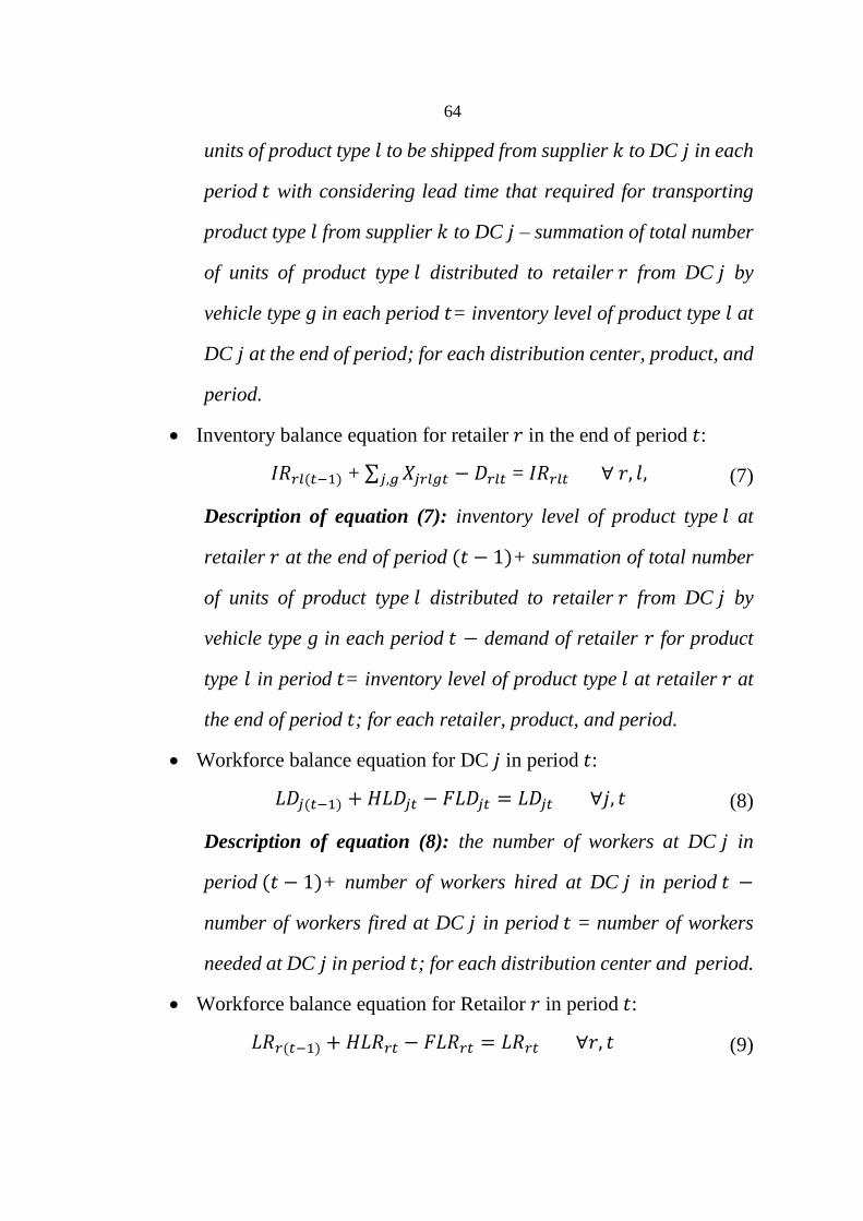
64

units of product type 𝑙 to be shipped from supplier 𝑘 to DC 𝑗 in each

period 𝑡 with considering lead time that required for transporting

product type 𝑙 from supplier 𝑘 to DC 𝑗 – summation of total number

of units of product type 𝑙 distributed to retailer 𝑟 from DC 𝑗 by

vehicle type g in each period 𝑡= inventory level of product type 𝑙 at

DC 𝑗 at the end of period; for each distribution center, product, and

period.

Inventory balance equation for retailer 𝑟 in the end of period 𝑡:

𝐼𝑅𝑟𝑙(𝑡−1) + ∑ 𝑋𝑗𝑟𝑙𝑔𝑡𝑗,𝑔 − 𝐷𝑟𝑙𝑡 = 𝐼𝑅𝑟𝑙𝑡 ∀ 𝑟, 𝑙, (7)

Description of equation (7): inventory level of product type 𝑙 at

retailer 𝑟 at the end of period (𝑡 − 1)+ summation of total number

of units of product type 𝑙 distributed to retailer 𝑟 from DC 𝑗 by

vehicle type g in each period 𝑡 − demand of retailer 𝑟 for product

type 𝑙 in period 𝑡= inventory level of product type 𝑙 at retailer 𝑟 at

the end of period 𝑡; for each retailer, product, and period.

Workforce balance equation for DC 𝑗 in period 𝑡:

𝐿𝐷𝑗(𝑡−1) + 𝐻𝐿𝐷𝑗𝑡 − 𝐹𝐿𝐷𝑗𝑡 = 𝐿𝐷𝑗𝑡 ∀𝑗, 𝑡 (8)

Description of equation (8): the number of workers at DC 𝑗 in

period (𝑡 − 1)+ number of workers hired at DC 𝑗 in period 𝑡 −

number of workers fired at DC 𝑗 in period 𝑡 = number of workers

needed at DC 𝑗 in period 𝑡; for each distribution center and period.

Workforce balance equation for Retailor 𝑟 in period 𝑡:

𝐿𝑅𝑟(𝑡−1) + 𝐻𝐿𝑅𝑟𝑡 − 𝐹𝐿𝑅𝑟𝑡 = 𝐿𝑅𝑟𝑡 ∀𝑟, 𝑡 (9)

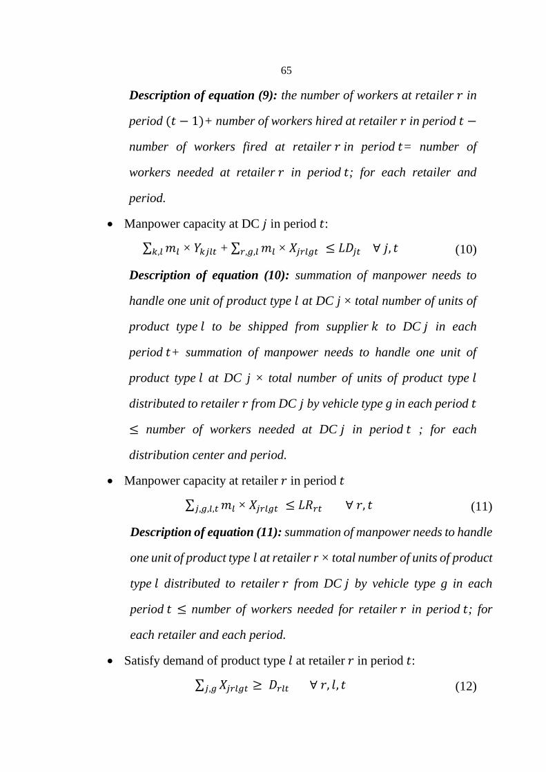
65

Description of equation (9): the number of workers at retailer 𝑟 in

period (𝑡 − 1)+ number of workers hired at retailer 𝑟 in period 𝑡 −

number of workers fired at retailer 𝑟 in period 𝑡= number of

workers needed at retailer 𝑟 in period 𝑡; for each retailer and

period.

Manpower capacity at DC 𝑗 in period 𝑡:

∑ 𝑚𝑙𝑘,𝑙 × 𝑌𝑘𝑗𝑙𝑡 + ∑ 𝑚𝑙𝑟,𝑔,𝑙 × 𝑋𝑗𝑟𝑙𝑔𝑡 ≤ 𝐿𝐷𝑗𝑡 ∀ 𝑗, 𝑡 (10)

Description of equation (10): summation of manpower needs to

handle one unit of product type 𝑙 at DC j × total number of units of

product type 𝑙 to be shipped from supplier 𝑘 to DC 𝑗 in each

period 𝑡+ summation of manpower needs to handle one unit of

product type 𝑙 at DC j × total number of units of product type 𝑙

distributed to retailer 𝑟 from DC 𝑗 by vehicle type g in each period 𝑡

≤ number of workers needed at DC 𝑗 in period 𝑡 ; for each

distribution center and period.

Manpower capacity at retailer 𝑟 in period 𝑡

∑ 𝑚𝑙𝑗,𝑔,𝑙,𝑡 × 𝑋𝑗𝑟𝑙𝑔𝑡 ≤ 𝐿𝑅𝑟𝑡 ∀ 𝑟, 𝑡 (11)

Description of equation (11): summation of manpower needs to handle

one unit of product type 𝑙 at retailer r × total number of units of product

type 𝑙 distributed to retailer 𝑟 from DC 𝑗 by vehicle type g in each

period 𝑡 ≤ number of workers needed for retailer 𝑟 in period 𝑡; for

each retailer and each period.

Satisfy demand of product type 𝑙 at retailer 𝑟 in period 𝑡:

∑ 𝑋𝑗𝑟𝑙𝑔𝑡 ≥ 𝐷𝑟𝑙𝑡 ∀ 𝑟, 𝑙, 𝑡𝑗,𝑔 (12)

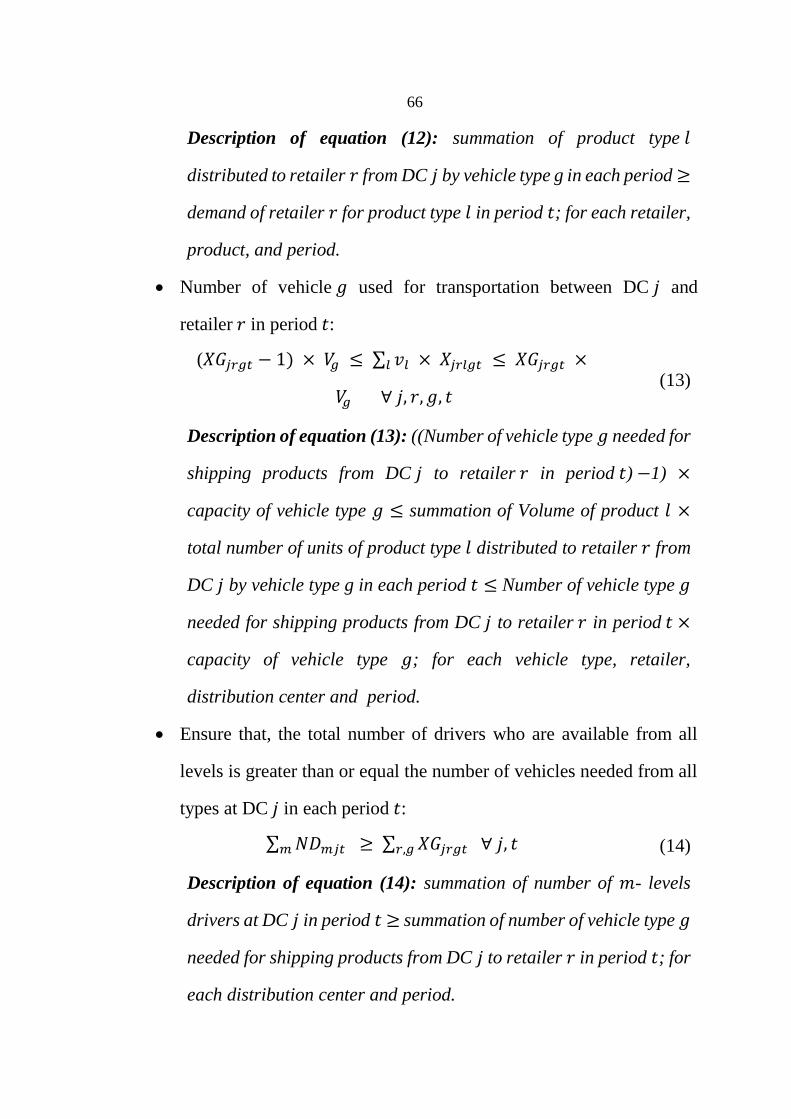
66

Description of equation (12): summation of product type 𝑙

distributed to retailer 𝑟 from DC 𝑗 by vehicle type g in each period ≥

demand of retailer 𝑟 for product type 𝑙 in period 𝑡; for each retailer,

product, and period.

Number of vehicle 𝑔 used for transportation between DC 𝑗 and

retailer 𝑟 in period 𝑡:

(𝑋𝐺𝑗𝑟𝑔𝑡 − 1) × 𝑉𝑔 ≤ ∑ 𝑣𝑙 × 𝑋𝑗𝑟𝑙𝑔𝑡𝑙 ≤ 𝑋𝐺𝑗𝑟𝑔𝑡 ×

𝑉𝑔 ∀ 𝑗, 𝑟, 𝑔, 𝑡 (13)

Description of equation (13): ((Number of vehicle type 𝑔 needed for

shipping products from DC 𝑗 to retailer 𝑟 in period 𝑡) −1) ×

capacity of vehicle type 𝑔 ≤ summation of Volume of product 𝑙 ×

total number of units of product type 𝑙 distributed to retailer 𝑟 from

DC 𝑗 by vehicle type g in each period 𝑡 ≤ Number of vehicle type 𝑔

needed for shipping products from DC 𝑗 to retailer 𝑟 in period 𝑡 ×

capacity of vehicle type 𝑔; for each vehicle type, retailer,

distribution center and period.

Ensure that, the total number of drivers who are available from all

levels is greater than or equal the number of vehicles needed from all

types at DC 𝑗 in each period 𝑡:

∑ 𝑁𝐷𝑚𝑗𝑡 ≥ 𝑚 ∑ 𝑋𝐺𝑗𝑟𝑔𝑡 ∀ 𝑗, 𝑡𝑟,𝑔 (14)

Description of equation (14): summation of number of 𝑚- levels

drivers at DC 𝑗 in period 𝑡 ≥ summation of number of vehicle type 𝑔

needed for shipping products from DC 𝑗 to retailer 𝑟 in period 𝑡; for

each distribution center and period.

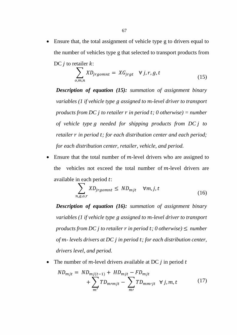
67

Ensure that, the total assignment of vehicle type g to drivers equal to

the number of vehicles type g that selected to transport products from

DC 𝑗 to retailer 𝑘:

∑ 𝑋𝐷𝑗𝑟𝑔𝑜𝑚𝑛𝑡 = 𝑋𝐺𝑗𝑟𝑔𝑡 ∀ 𝑗, 𝑟, 𝑔, 𝑡

𝑜,𝑚,𝑛

(15)

Description of equation (15): summation of assignment binary

variables (1 if vehicle type 𝑔 assigned to 𝑚-level driver to transport

products from DC 𝑗 to retailer 𝑟 in period 𝑡; 0 otherwise) = number

of vehicle type 𝑔 needed for shipping products from DC 𝑗 to

retailer 𝑟 in period 𝑡; for each distribution center and each period;

for each distribution center, retailer, vehicle, and period.

Ensure that the total number of 𝑚-level drivers who are assigned to

the vehicles not exceed the total number of 𝑚-level drivers are

available in each period 𝑡:

∑ 𝑋𝐷𝑗𝑟𝑔𝑜𝑚𝑛𝑡 ≤ 𝑁𝐷𝑚𝑗𝑡 ∀𝑚, 𝑗, 𝑡

𝑛,𝑔,𝑜,𝑟

(16)

Description of equation (16): summation of assignment binary

variables (1 if vehicle type 𝑔 assigned to 𝑚-level driver to transport

products from DC 𝑗 to retailer 𝑟 in period 𝑡; 0 otherwise) ≤ number

of 𝑚- levels drivers at DC 𝑗 in period 𝑡; for each distribution center,

drivers level, and period.

The number of 𝑚-level drivers available at DC 𝑗 in period 𝑡

𝑁𝐷𝑚𝑗𝑡 = 𝑁𝐷𝑚𝑗(𝑡−1) + 𝐻𝐷𝑚𝑗𝑡 − 𝐹𝐷𝑚𝑗𝑡

+ ∑ 𝑇𝐷𝑚′𝑚𝑗𝑡 − ∑ 𝑇𝐷𝑚𝑚′𝑗𝑡 ∀ 𝑗, 𝑚, 𝑡

𝑚′𝑚′

(17)

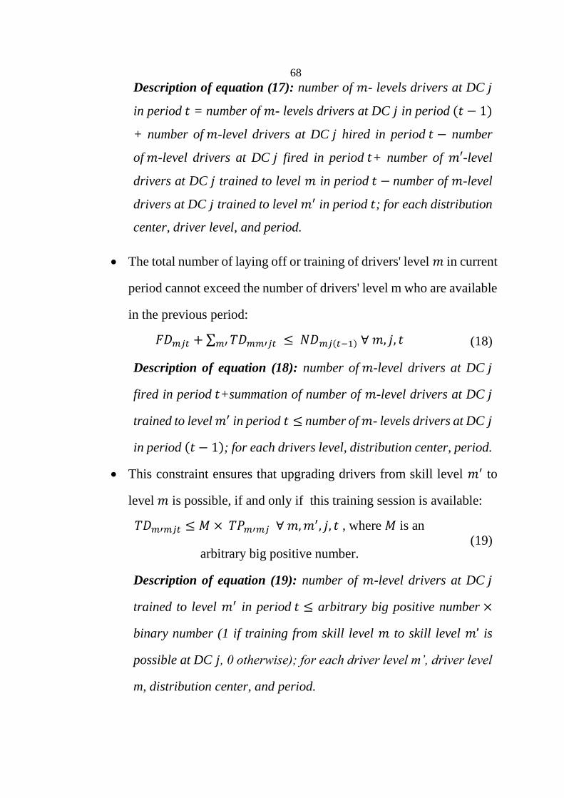
68

Description of equation (17): number of 𝑚- levels drivers at DC 𝑗

in period 𝑡 = number of 𝑚- levels drivers at DC 𝑗 in period (𝑡 − 1)

+ number of 𝑚-level drivers at DC 𝑗 hired in period 𝑡 − number

of 𝑚-level drivers at DC 𝑗 fired in period 𝑡+ number of 𝑚′-level

drivers at DC 𝑗 trained to level 𝑚 in period 𝑡 − number of 𝑚-level

drivers at DC 𝑗 trained to level 𝑚′ in period 𝑡; for each distribution

center, driver level, and period.

The total number of laying off or training of drivers' level 𝑚 in current

period cannot exceed the number of drivers' level m who are available

in the previous period:

𝐹𝐷𝑚𝑗𝑡 + ∑ 𝑇𝐷𝑚𝑚′𝑗𝑡 𝑚′ ≤ 𝑁𝐷𝑚𝑗(𝑡−1) ∀ 𝑚, 𝑗, 𝑡 (18)

Description of equation (18): number of 𝑚-level drivers at DC 𝑗

fired in period 𝑡+summation of number of 𝑚-level drivers at DC 𝑗

trained to level 𝑚′ in period 𝑡 ≤ number of 𝑚- levels drivers at DC 𝑗

in period (𝑡 − 1); for each drivers level, distribution center, period.

This constraint ensures that upgrading drivers from skill level 𝑚′ to

level 𝑚 is possible, if and only if this training session is available:

𝑇𝐷𝑚′𝑚𝑗𝑡 ≤ 𝑀 × 𝑇𝑃𝑚′𝑚𝑗 ∀ 𝑚, 𝑚′, 𝑗, 𝑡 , where 𝑀 is an

arbitrary big positive number. (19)

Description of equation (19): number of 𝑚-level drivers at DC 𝑗

trained to level 𝑚′ in period 𝑡 ≤ arbitrary big positive number ×

binary number (1 if training from skill level 𝑚 to skill level 𝑚’ is

possible at DC 𝑗, 0 otherwise); for each driver level m’, driver level

m, distribution center, and period.

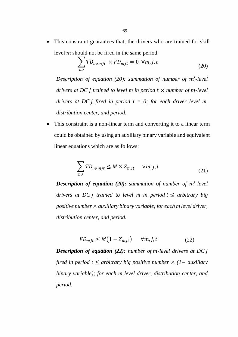
69

This constraint guarantees that, the drivers who are trained for skill

level 𝑚 should not be fired in the same period.

∑ 𝑇𝐷𝑚′𝑚𝑗𝑡 × 𝐹𝐷𝑚𝑗𝑡 = 0 ∀𝑚, 𝑗, 𝑡

𝑚′

(20)

Description of equation (20): summation of number of 𝑚′-level

drivers at DC 𝑗 trained to level m in period 𝑡 × number of 𝑚-level

drivers at DC 𝑗 fired in period t = 0; for each driver level m,

distribution center, and period.

This constraint is a non-linear term and converting it to a linear term

could be obtained by using an auxiliary binary variable and equivalent

linear equations which are as follows:

∑ 𝑇𝐷𝑚′𝑚𝑗𝑡 ≤ 𝑀 × 𝑍𝑚𝑗𝑡 ∀𝑚, 𝑗, 𝑡

𝑚′

(21)

Description of equation (20): summation of number of 𝑚′-level

drivers at DC 𝑗 trained to level m in period 𝑡 ≤ arbitrary big

positive number × auxiliary binary variable; for each m level driver,

distribution center, and period.

𝐹𝐷𝑚𝑗𝑡 ≤ 𝑀(1 − 𝑍𝑚𝑗𝑡) ∀𝑚, 𝑗, 𝑡 (22)

Description of equation (22): number of 𝑚-level drivers at DC 𝑗

fired in period t ≤ arbitrary big positive number × (1− auxiliary

binary variable); for each m level driver, distribution center, and

period.

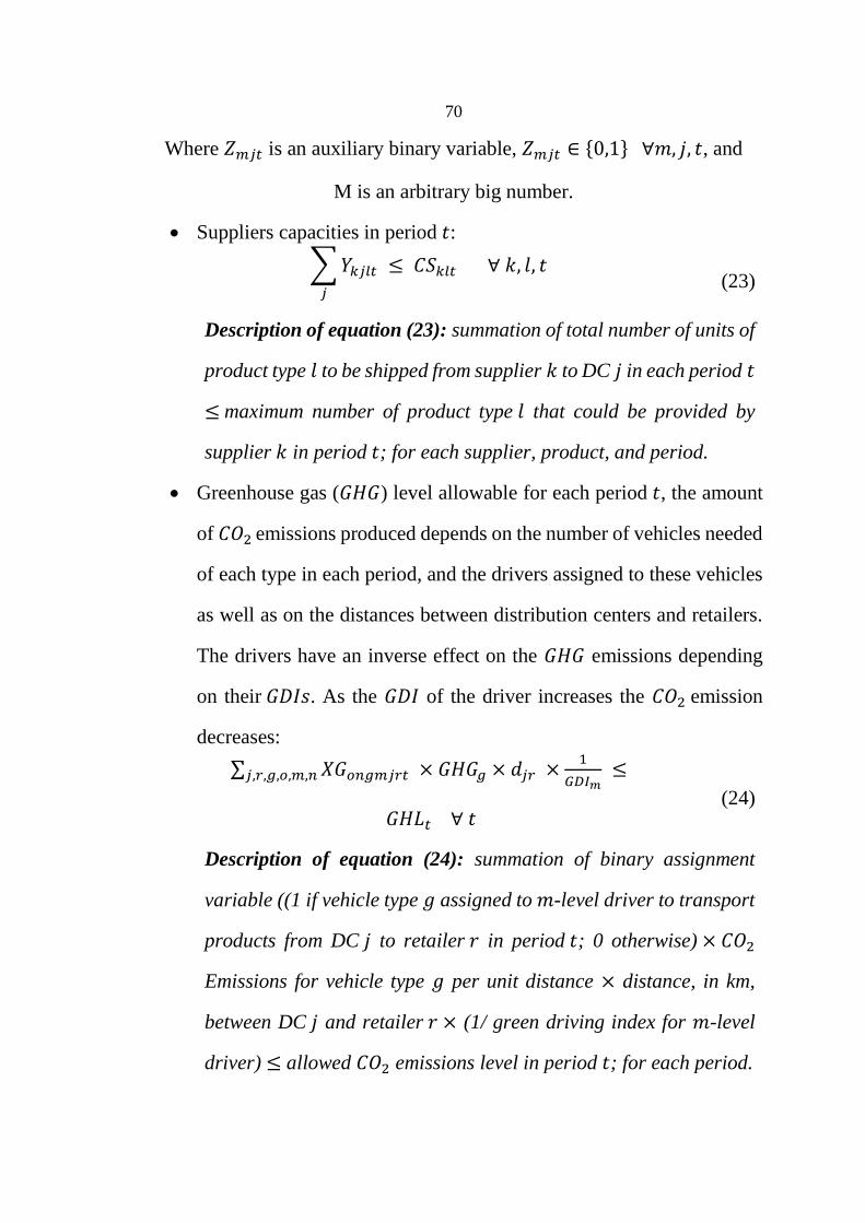
70

Where 𝑍𝑚𝑗𝑡 is an auxiliary binary variable, 𝑍𝑚𝑗𝑡 ∈ {0,1} ∀𝑚, 𝑗, 𝑡, and

M is an arbitrary big number.

Suppliers capacities in period 𝑡:

∑ 𝑌𝑘𝑗𝑙𝑡 ≤ 𝐶𝑆𝑘𝑙𝑡

𝑗

∀ 𝑘, 𝑙, 𝑡 (23)

Description of equation (23): summation of total number of units of

product type 𝑙 to be shipped from supplier 𝑘 to DC 𝑗 in each period 𝑡

≤ maximum number of product type 𝑙 that could be provided by

supplier 𝑘 in period 𝑡; for each supplier, product, and period.

Greenhouse gas (𝐺𝐻𝐺) level allowable for each period 𝑡, the amount

of 𝐶𝑂2 emissions produced depends on the number of vehicles needed

of each type in each period, and the drivers assigned to these vehicles

as well as on the distances between distribution centers and retailers.

The drivers have an inverse effect on the 𝐺𝐻𝐺 emissions depending

on their 𝐺𝐷𝐼𝑠. As the 𝐺𝐷𝐼 of the driver increases the 𝐶𝑂2 emission

decreases:

∑ 𝑋𝐺𝑜𝑛𝑔𝑚𝑗𝑟𝑡 × 𝐺𝐻𝐺𝑔 × 𝑑𝑗𝑟 ×1

𝐺𝐷𝐼𝑚 ≤𝑗,𝑟,𝑔,𝑜,𝑚,𝑛

𝐺𝐻𝐿𝑡 ∀ 𝑡 (24)

Description of equation (24): summation of binary assignment

variable ((1 if vehicle type 𝑔 assigned to 𝑚-level driver to transport

products from DC 𝑗 to retailer 𝑟 in period 𝑡; 0 otherwise) × 𝐶𝑂2

Emissions for vehicle type 𝑔 per unit distance × distance, in km,

between DC 𝑗 and retailer 𝑟 × (1/ green driving index for 𝑚-level

driver) ≤ allowed 𝐶𝑂2 emissions level in period 𝑡; for each period.

71

The number of product type 𝑙 shipped from DC 𝑗 to retail store 𝑟, does

not exceed the available of product 𝑙 at the DC 𝑗 in period 𝑡:

𝐼𝐷𝑗𝑙(𝑡−1) + ∑ 𝑌𝑘𝑗𝑙𝑡 ≥ ∑ 𝑋𝑗𝑟𝑙𝑔𝑡 ∀ 𝑗, 𝑙, 𝑡𝑟,𝑔𝑘 (25)

Description of equation (25): inventory level of product type 𝑙 at

DC 𝑗 at the end of period 𝑡 + summation of total number of units of

product type 𝑙 to be shipped from supplier 𝑘 to DC 𝑗 in each period 𝑡

≥ summation of total number of units of product type 𝑙 distributed

to retailer 𝑟 from DC 𝑗 by vehicle type g in each period 𝑡; for each

distribution center, product, and period.

The constraint ensures that, the inventory level at DC cannot exceed

the available storage capacity at DC 𝑗 in each period:

∑ 𝑣𝑙 × 𝐼𝐷𝑗𝑙𝑡 ≤ 𝑤𝑗

𝑙

∀ 𝑗, 𝑡 (26)

Description of equation (26): summation of Volume of product 𝑙 ×

inventory level of product type 𝑙 at DC 𝑗 at the end of period 𝑡 ≤

product storage capacity of DC 𝑗; for each distribution center and

period.

The constraint ensures that, the inventory level at retailer 𝑟 cannot

exceed the available storage capacity at retailer 𝑟 in each period 𝑡:

∑ 𝑣𝑙 × 𝐼𝑅𝑟𝑙𝑡 ≤ 𝑅𝑟

𝑙

∀ 𝑟, 𝑡 (27)

Description of equation (26): summation of Volume of product 𝑙 ×

product storage capacity of retailer 𝑟 ≤ inventory level of product

type 𝑙 at retailer 𝑟 at the end of period 𝑡; for each retailer and

period.

72

Non-negativity and integers constraints:

𝑋𝑗𝑟𝑙𝑔𝑡, 𝑋𝐺𝑗𝑟𝑔𝑡, 𝑌𝑘𝑗𝑙𝑡, 𝐼𝐷𝑗𝑙𝑡 , 𝐼𝑅𝑟𝑙𝑡, 𝑇𝐷𝑚𝑚′𝑗𝑡, 𝐹𝐷𝑚𝑗𝑡 , 𝐻𝐷𝑚𝑗𝑡 , 𝑁𝐷𝑚𝑗𝑡 , 𝐿𝐷𝑗𝑡 , 𝐿𝑅𝑟𝑡, 𝐻𝐿𝐷𝑗𝑡 , 𝐹𝐿𝐷𝑗𝑡

, 𝐻𝐿𝑅𝑟𝑡 , 𝐹𝐿𝑅𝑟𝑡 ≥ 0 𝑎𝑛𝑑 𝑖𝑛𝑡𝑒𝑔𝑒𝑟𝑠

𝑋𝐷𝑜𝑛𝑔𝑚𝑗𝑟𝑡, 𝑇𝑃𝑚′𝑚𝑗𝑡 , 𝑍𝑚𝑗𝑡 ∈ {0,1}

3.4 Summary

In this chapter, the proposed model for Green Supply Chain Management

(GSCM) was described. This model was formulated as a MINLP and then

converted to a linear one. The developed model deals with multi-site, multi

product and multi period APP in GSCM. The aim of this model is to

minimize the total costs across the entire supply chain network. In addition

to guarantee that the 𝐶𝑂2 emissions do not exceed the predetermined level.

This model contributes to the literature with a novel approach that integrating

drivers’ differences in managing and planning GSC at tactical and

operational levels, with aims to optimal selection of drivers, training them

and then introducing the optimum assignment between drivers, vehicles and

the destinations (i.e. retail stores) in order to reduce the total cost and

𝐶𝑂2 emission across the supply chain network.

73

Chapter Four

Model Results

74

Chapter Four

Model Results

4.1 Overview

This chapter presents a numerical study to demonstrate the validity of the

proposed model. In section 4.1, the description of the hypothetical problem

will be shown. The results of hypothetical numerical example will be

generated by using Matlab 2015a program. In section 4.2.1, some

characteristics of Matlab program and the “intlinprog” solver will be

presented. Finally, section 4.2.2 presents and discusses the numerical results

of solving the hypothetical example.

4.2 Hypothetical Data

The analysis was based upon data which was derived from the literature and

addition to hypothetical data that covered all parameters and data needed.

The multi-site retail stores company intended to plan its APP taking 3 periods

as a planning horizon, with a single type of product. The supply chain

network consist of two suppliers S1 and S2, two distribution centers DC1

and DC2, and two retailers R1 and R2, all supply chain sites spread out

geographically. We assumed that the demand during planning horizon is

known, as shown in Table 4.1. The storage capacity and holding cost at

retailers and distances between retailers and DCs are also presented in Table

4.1. Inventory holding cost per unit of product and storage capacities at DCs,

and the limit of greenhouse gas emission allowable per each period are

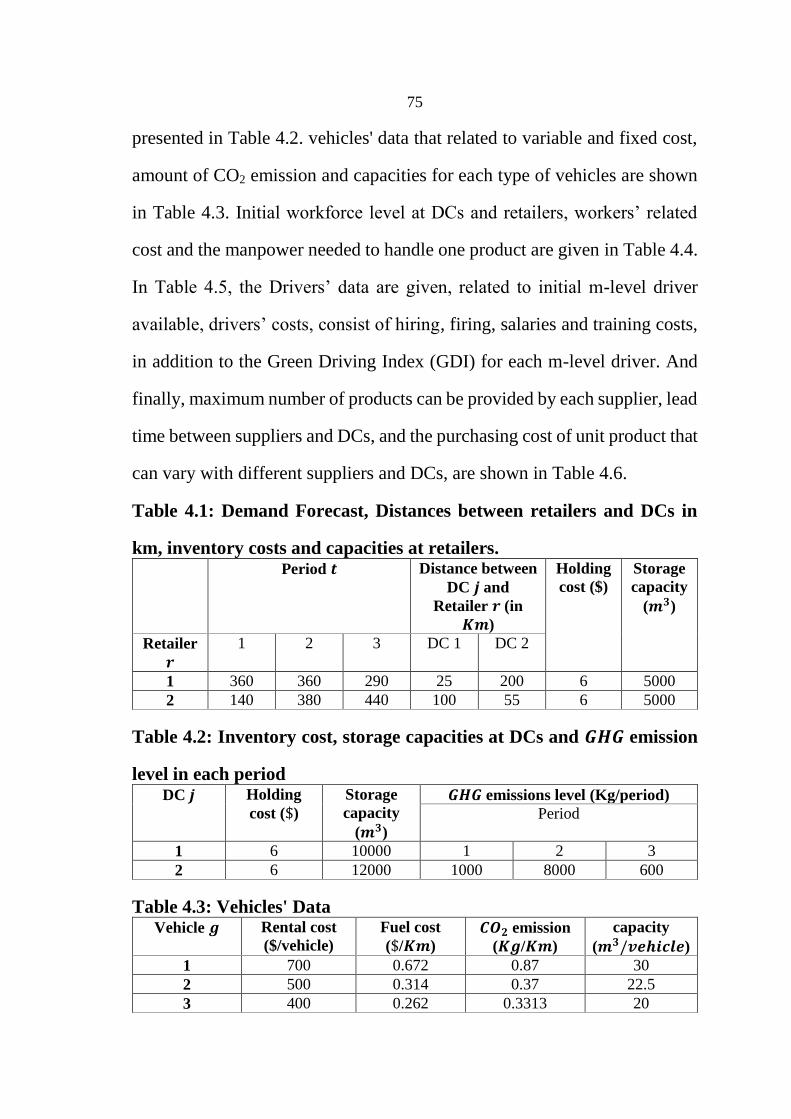
75

presented in Table 4.2. vehicles' data that related to variable and fixed cost,

amount of CO2 emission and capacities for each type of vehicles are shown

in Table 4.3. Initial workforce level at DCs and retailers, workers’ related

cost and the manpower needed to handle one product are given in Table 4.4.

In Table 4.5, the Drivers’ data are given, related to initial m-level driver

available, drivers’ costs, consist of hiring, firing, salaries and training costs,

in addition to the Green Driving Index (GDI) for each m-level driver. And

finally, maximum number of products can be provided by each supplier, lead

time between suppliers and DCs, and the purchasing cost of unit product that

can vary with different suppliers and DCs, are shown in Table 4.6.

Table 4.1: Demand Forecast, Distances between retailers and DCs in

km, inventory costs and capacities at retailers. Period 𝒕 Distance between

DC 𝒋 and

Retailer 𝒓 (in

𝑲𝒎)

Holding

cost ($)

Storage

capacity

(𝒎𝟑)

Retailer

𝒓

1 2 3 DC 1 DC 2

1 360 360 290 25 200 6 5000

2 140 380 440 100 55 6 5000

Table 4.2: Inventory cost, storage capacities at DCs and 𝑮𝑯𝑮 emission

level in each period DC 𝒋 Holding

cost ($)

Storage

capacity

(𝒎𝟑)

𝑮𝑯𝑮 emissions level (Kg/period)

Period

1 6 10000 1 2 3

2 6 12000 1000 8000 600

Table 4.3: Vehicles' Data Vehicle 𝒈 Rental cost

($/vehicle)

Fuel cost

($/𝑲𝒎)

𝑪𝑶𝟐 emission

(𝑲𝒈/𝑲𝒎)

capacity

(𝒎𝟑/𝒗𝒆𝒉𝒊𝒄𝒍𝒆)

1 700 0.672 0.87 30

2 500 0.314 0.37 22.5

3 400 0.262 0.3313 20

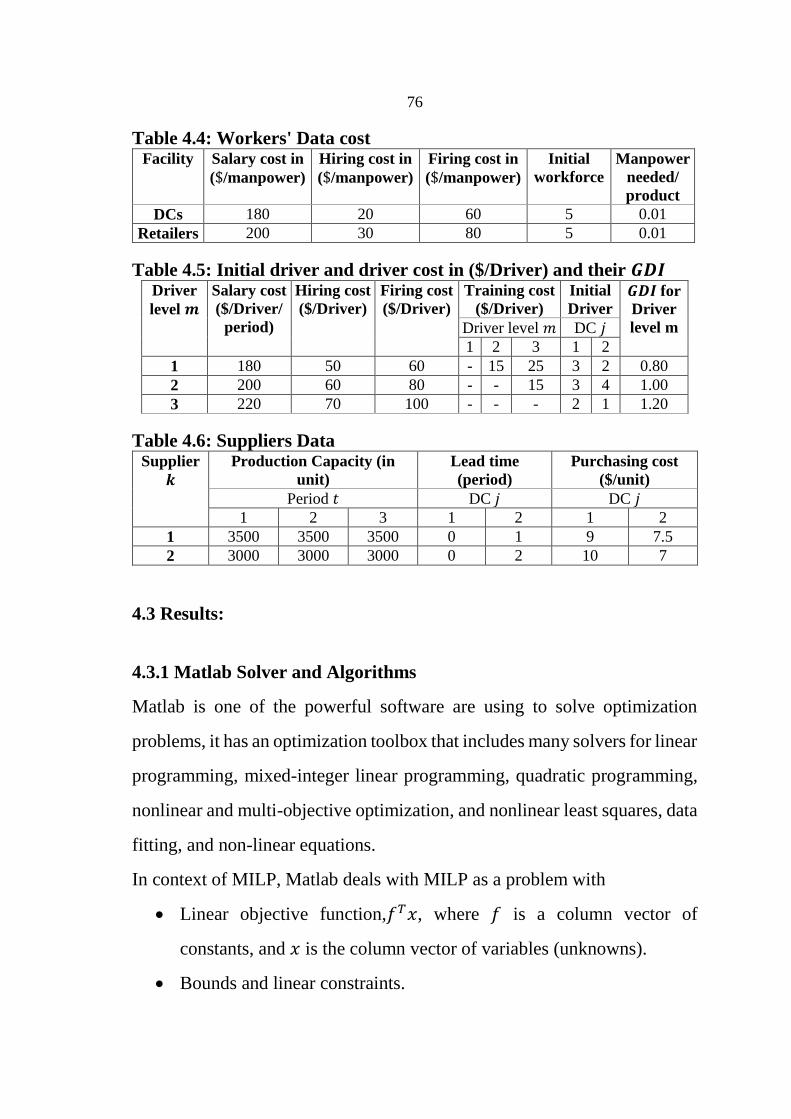
76

Table 4.4: Workers' Data cost Facility Salary cost in

($/manpower)

Hiring cost in

($/manpower)

Firing cost in

($/manpower)

Initial

workforce

Manpower

needed/

product

DCs 180 20 60 5 0.01

Retailers 200 30 80 5 0.01

Table 4.5: Initial driver and driver cost in ($/Driver) and their 𝑮𝑫𝑰 Driver

level 𝒎

Salary cost

($/Driver/

period)

Hiring cost

($/Driver)

Firing cost

($/Driver)

Training cost

($/Driver)

Initial

Driver

𝑮𝑫𝑰 for

Driver

level m Driver level 𝑚 DC 𝑗

1 2 3 1 2

1 180 50 60 - 15 25 3 2 0.80

2 200 60 80 - - 15 3 4 1.00

3 220 70 100 - - - 2 1 1.20

Table 4.6: Suppliers Data Supplier

𝒌

Production Capacity (in

unit)

Lead time

(period)

Purchasing cost

($/unit)

Period 𝑡 DC 𝑗 DC 𝑗

1 2 3 1 2 1 2

1 3500 3500 3500 0 1 9 7.5

2 3000 3000 3000 0 2 10 7

4.3 Results:

4.3.1 Matlab Solver and Algorithms

Matlab is one of the powerful software are using to solve optimization

problems, it has an optimization toolbox that includes many solvers for linear

programming, mixed-integer linear programming, quadratic programming,

nonlinear and multi-objective optimization, and nonlinear least squares, data

fitting, and non-linear equations.

In context of MILP, Matlab deals with MILP as a problem with

Linear objective function,𝑓𝑇𝑥, where 𝑓 is a column vector of

constants, and 𝑥 is the column vector of variables (unknowns).

Bounds and linear constraints.

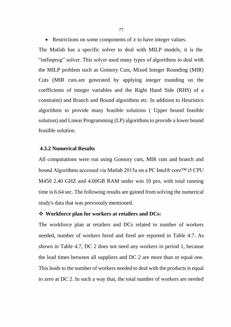
77

Restrictions on some components of 𝑥 to have integer values.

The Matlab has a specific solver to deal with MILP models, it is the

“intlinprog” solver. This solver used many types of algorithms to deal with

the MILP problem such as Gomory Cuts, Mixed Integer Rounding (MIR)

Cuts (MIR cuts are generated by applying integer rounding on the

coefficients of integer variables and the Right Hand Side (RHS) of a

constraint) and Branch and Bound algorithms etc. In addition to Heuristics

algorithms to provide many feasible solutions ( Upper bound feasible

solution) and Linear Programming (LP) algorithms to provide a lower bound

feasible solution.

4.3.2 Numerical Results

All computations were run using Gomory cuts, MIR cuts and branch and

bound Algorithms accessed via Matlab 2015a on a PC Intel® core™ i5 CPU

M450 2.40 GHZ and 4.00GB RAM under win 10 pro, with total running

time is 6.64 sec. The following results are gained from solving the numerical

study's data that was previously mentioned.

Workforce plan for workers at retailers and DCs:

The workforce plan at retailers and DCs related to number of workers

needed, number of workers hired and fired are reported in Table 4.7. As

shown in Table 4.7, DC 2 does not need any workers in period 1, because

the lead times between all suppliers and DC 2 are more than or equal one.

This leads to the number of workers needed to deal with the products is equal

to zero at DC 2. In such a way that, the total number of workers are needed

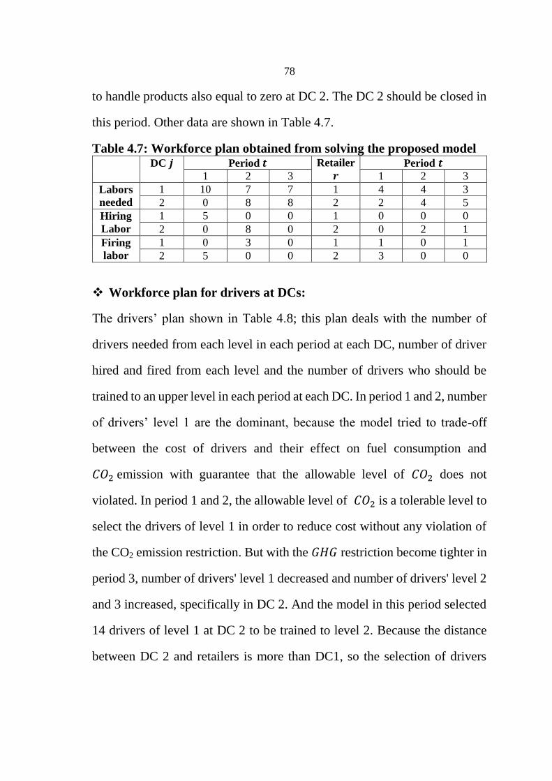
78

to handle products also equal to zero at DC 2. The DC 2 should be closed in

this period. Other data are shown in Table 4.7.

Table 4.7: Workforce plan obtained from solving the proposed model DC 𝒋 Period 𝒕 Retailer

𝒓

Period 𝒕

1 2 3 1 2 3

Labors

needed

1 10 7 7 1 4 4 3

2 0 8 8 2 2 4 5

Hiring

Labor

1 5 0 0 1 0 0 0

2 0 8 0 2 0 2 1

Firing

labor

1 0 3 0 1 1 0 1

2 5 0 0 2 3 0 0

Workforce plan for drivers at DCs:

The drivers’ plan shown in Table 4.8; this plan deals with the number of

drivers needed from each level in each period at each DC, number of driver

hired and fired from each level and the number of drivers who should be

trained to an upper level in each period at each DC. In period 1 and 2, number

of drivers’ level 1 are the dominant, because the model tried to trade-off

between the cost of drivers and their effect on fuel consumption and

𝐶𝑂2 emission with guarantee that the allowable level of 𝐶𝑂2 does not

violated. In period 1 and 2, the allowable level of 𝐶𝑂2 is a tolerable level to

select the drivers of level 1 in order to reduce cost without any violation of

the CO2 emission restriction. But with the 𝐺𝐻𝐺 restriction become tighter in

period 3, number of drivers' level 1 decreased and number of drivers' level 2

and 3 increased, specifically in DC 2. And the model in this period selected

14 drivers of level 1 at DC 2 to be trained to level 2. Because the distance

between DC 2 and retailers is more than DC1, so the selection of drivers

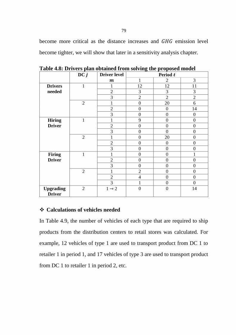
79

become more critical as the distance increases and 𝐺𝐻𝐺 emission level

become tighter, we will show that later in a sensitivity analysis chapter.

Table 4.8: Drivers plan obtained from solving the proposed model DC 𝒋 Driver level

𝒎

Period 𝒕

1 2 3

Drivers

needed

1 1 12 12 11

2 3 3 3

3 2 2 2

2 1 0 20 6

2 0 0 14

3 0 0 0

Hiring

Driver

1 1 9 0 0

2 0 0 0

3 0 0 0

2 1 0 20 0

2 0 0 0

3 0 0 0

Firing

Driver

1 1 0 0 1

2 0 0 0

3 0 0 0

2 1 2 0 0

2 4 0 0

3 1 0 0

Upgrading

Driver

2 1 → 2 0 0 14

Calculations of vehicles needed

In Table 4.9, the number of vehicles of each type that are required to ship

products from the distribution centers to retail stores was calculated. For

example, 12 vehicles of type 1 are used to transport product from DC 1 to

retailer 1 in period 1, and 17 vehicles of type 3 are used to transport product

from DC 1 to retailer 1 in period 2, etc.

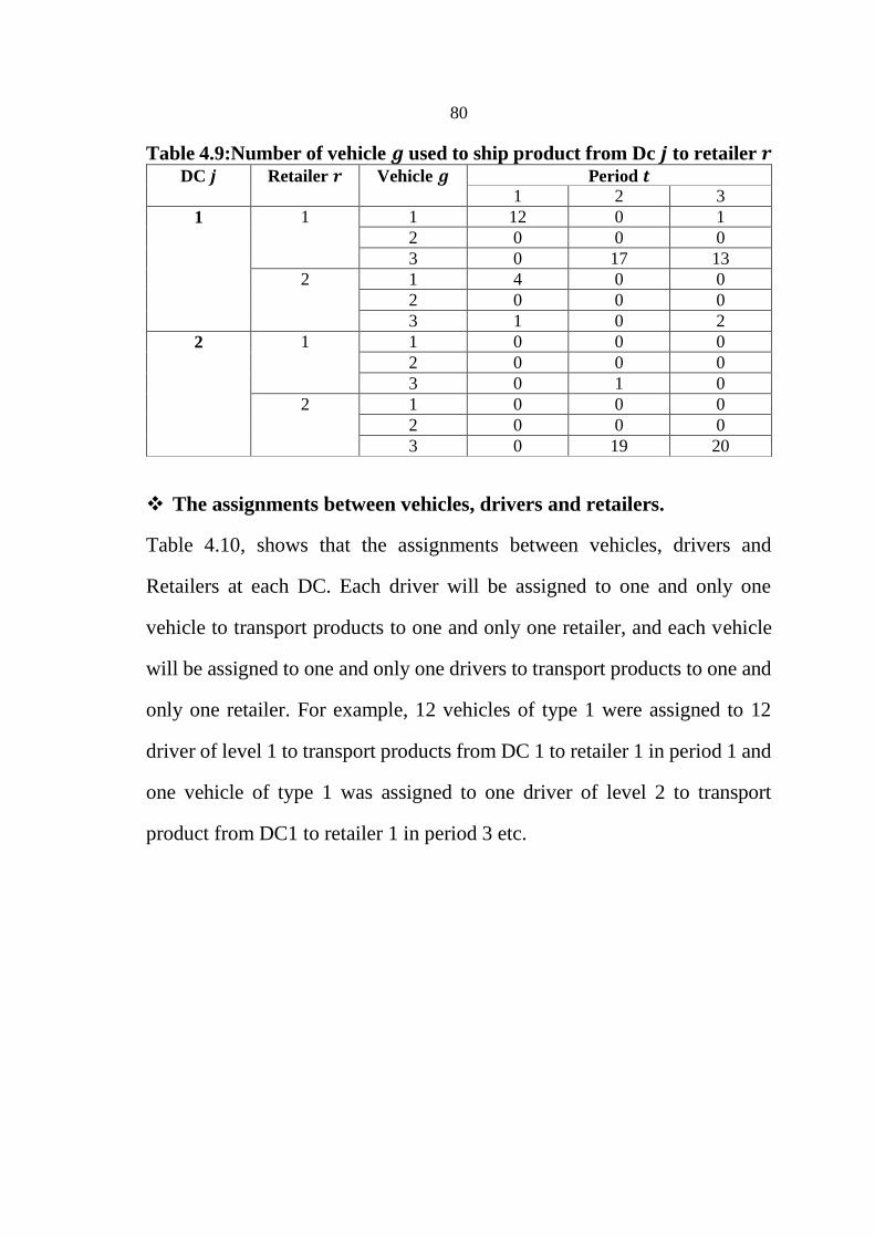
80

Table 4.9:Number of vehicle 𝒈 used to ship product from Dc 𝒋 to retailer 𝒓 DC 𝒋 Retailer 𝒓 Vehicle 𝒈 Period 𝒕

1 2 3

1 1 1 12 0 1

2 0 0 0

3 0 17 13

2 1 4 0 0

2 0 0 0

3 1 0 2

2 1 1 0 0 0

2 0 0 0

3 0 1 0

2 1 0 0 0

2 0 0 0

3 0 19 20

The assignments between vehicles, drivers and retailers.

Table 4.10, shows that the assignments between vehicles, drivers and

Retailers at each DC. Each driver will be assigned to one and only one

vehicle to transport products to one and only one retailer, and each vehicle

will be assigned to one and only one drivers to transport products to one and

only one retailer. For example, 12 vehicles of type 1 were assigned to 12

driver of level 1 to transport products from DC 1 to retailer 1 in period 1 and

one vehicle of type 1 was assigned to one driver of level 2 to transport

product from DC1 to retailer 1 in period 3 etc.

81

Table 4.10: Number of assignments between driver level 𝒎, vehicle type

𝒈 and retailer 𝒓 at Dc 𝒋 in each period 𝒕. DC 𝒋 Retailer 𝒓 Vehicle 𝒈 Driver

level 𝒎

Period 𝒕

1 2 3

1 1 1 1 12 0 0

2 0 0 1

3 0 0 0

2 1 0 0 0

2 0 0 0

3 0 0 0

3 1 0 12 11

2 0 3 2

3 0 2 0

2 1 1 0 0 0

2 2 0 0

3 2 0 0

2 1 0 0 0

2 0 0 0

3 0 0 0

3 1 0 0 0

2 1 0 0

3 0 0 2

2 1 1 1 0 0 0

2 0 0 0

3 0 0 0

2 1 0 0 0

2 0 0 0

3 0 0 0

3 1 0 1 0

2 0 0 0

3 0 0 0

2 1 1 0 0 0

2 0 0 0

3 0 0 0

2 1 0 0 0

2 0 0 0

3 0 0 0

3 1 0 19 6

2 0 0 14

3 0 0 0

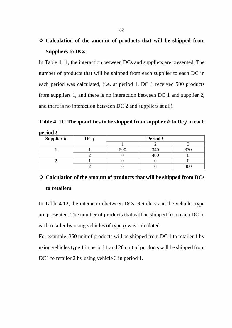
82

Calculation of the amount of products that will be shipped from

Suppliers to DCs

In Table 4.11, the interaction between DCs and suppliers are presented. The

number of products that will be shipped from each supplier to each DC in

each period was calculated, (i.e. at period 1, DC 1 received 500 products

from suppliers 1, and there is no interaction between DC 1 and supplier 2,

and there is no interaction between DC 2 and suppliers at all).

Table 4. 11: The quantities to be shipped from supplier 𝒌 to Dc 𝒋 in each

period 𝒕 Supplier 𝒌 DC 𝒋 Period 𝒕

1 2 3

1 1 500 340 330

2 0 400 0

2 1 0 0 0

2 0 0 400

Calculation of the amount of products that will be shipped from DCs

to retailers

In Table 4.12, the interaction between DCs, Retailers and the vehicles type

are presented. The number of products that will be shipped from each DC to

each retailer by using vehicles of type 𝑔 was calculated.

For example, 360 unit of products will be shipped from DC 1 to retailer 1 by

using vehicles type 1 in period 1 and 20 unit of products will be shipped from

DC1 to retailer 2 by using vehicle 3 in period 1.

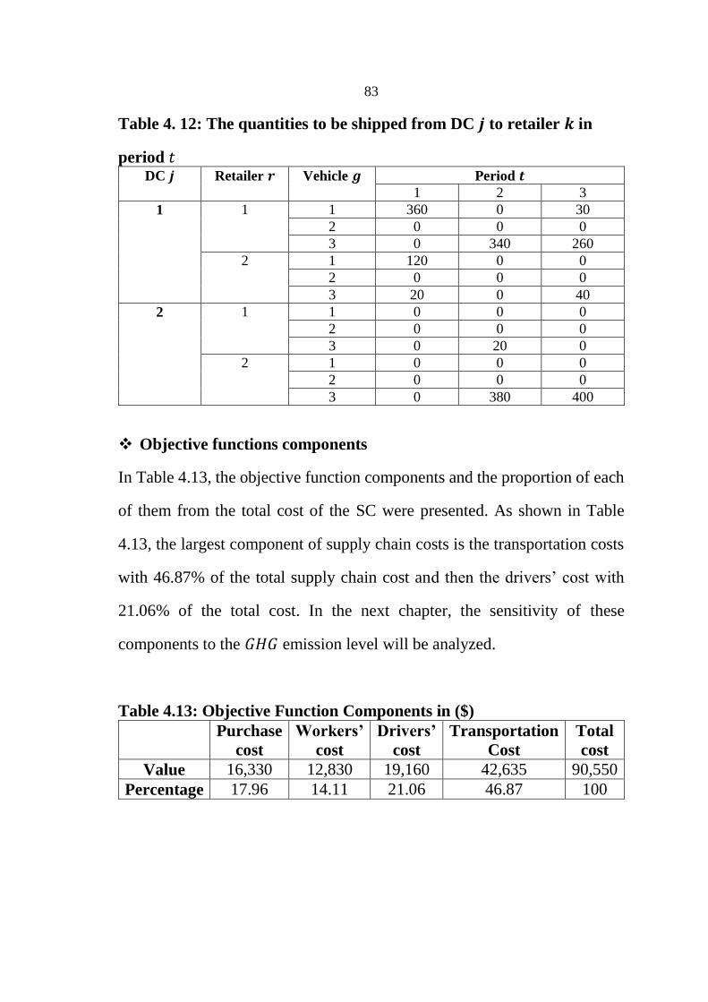
83

Table 4. 12: The quantities to be shipped from DC 𝒋 to retailer 𝒌 in

period 𝑡 DC 𝒋 Retailer 𝒓 Vehicle 𝒈 Period 𝒕

1 2 3

1 1 1 360 0 30

2 0 0 0

3 0 340 260

2 1 120 0 0

2 0 0 0

3 20 0 40

2 1 1 0 0 0

2 0 0 0

3 0 20 0

2 1 0 0 0

2 0 0 0

3 0 380 400

Objective functions components

In Table 4.13, the objective function components and the proportion of each

of them from the total cost of the SC were presented. As shown in Table

4.13, the largest component of supply chain costs is the transportation costs

with 46.87% of the total supply chain cost and then the drivers’ cost with

21.06% of the total cost. In the next chapter, the sensitivity of these

components to the 𝐺𝐻𝐺 emission level will be analyzed.

Table 4.13: Objective Function Components in ($)

Purchase

cost

Workers’

cost

Drivers’

cost

Transportation

Cost

Total

cost

Value 16,330 12,830 19,160 42,635 90,550

Percentage 17.96 14.11 21.06 46.87 100

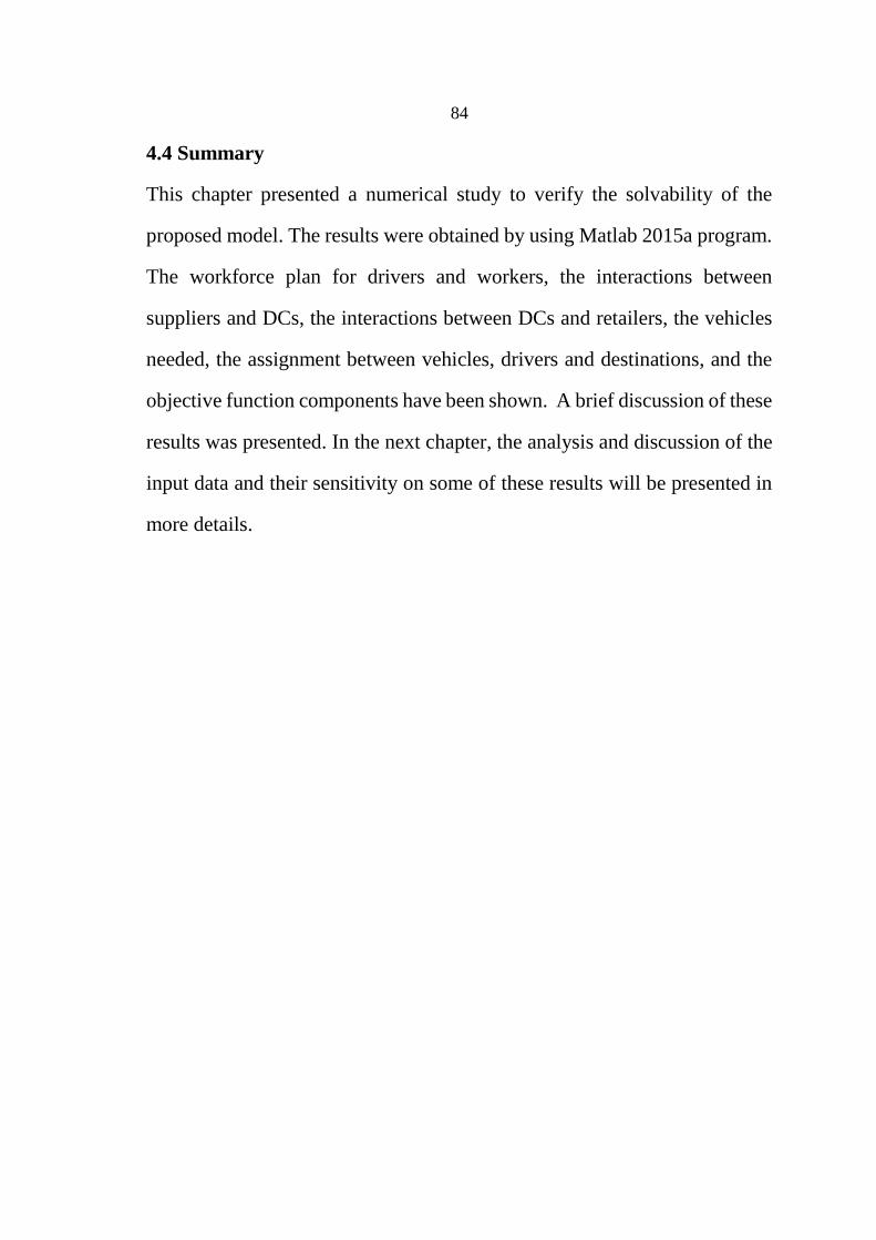
84

4.4 Summary

This chapter presented a numerical study to verify the solvability of the

proposed model. The results were obtained by using Matlab 2015a program.

The workforce plan for drivers and workers, the interactions between

suppliers and DCs, the interactions between DCs and retailers, the vehicles

needed, the assignment between vehicles, drivers and destinations, and the

objective function components have been shown. A brief discussion of these

results was presented. In the next chapter, the analysis and discussion of the

input data and their sensitivity on some of these results will be presented in

more details.

85

Chapter Five

Sensitivity Analysis

86

Chapter Five

Sensitivity Analysis

5.1 Overview

In this chapter the sensitivity analysis will be conducted, which means that

the numerical parameters used in solving the model will be examined and

then the results obtained will be analyzed. Conducting sensitivity analysis

will be on the three important parameters such as the 𝐺𝐻𝐺 emission level,

the distances between DCs and retailers and the cost of drivers. After

identifying these sensitive parameters, the sensitivity analysis will be

conducted to see how much the model’s results are sensitive to changing in

these parameters. So, the effect of the allowable GHG emissions level on the

total costs and the selection of drivers, the effect of distances between DCs

and retailers on the selection of drivers, and the effect of differences in cost

between drivers on the selection of drivers will be analyzed.

5.2 Conducting a Sensitivity Analysis on the 𝑮𝑯𝑮 emission level

In this section, we conduct a sensitivity analysis on the allowable GHG

emissions level and its effect on the total cost and the selection of drivers.

5.2.1 The effect of 𝑮𝑯𝑮 emission level on the total costs of supply chain

We conducted a sensitivity analysis in this section, to examine the change in

total cost at each level of GHG emission. The right hand side of GHG

emission is our concern. At first, we put a large value for the allowable

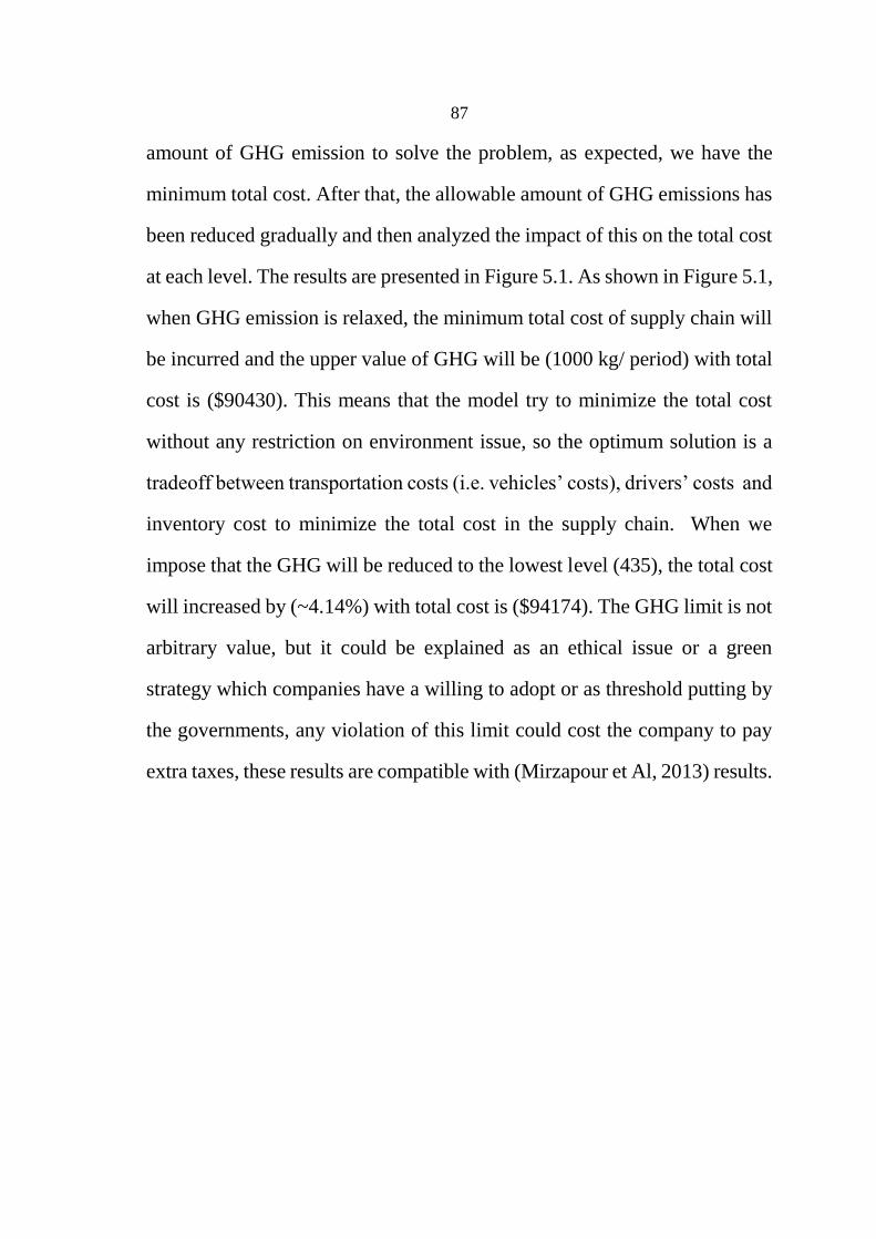
87

amount of GHG emission to solve the problem, as expected, we have the

minimum total cost. After that, the allowable amount of GHG emissions has

been reduced gradually and then analyzed the impact of this on the total cost

at each level. The results are presented in Figure 5.1. As shown in Figure 5.1,

when GHG emission is relaxed, the minimum total cost of supply chain will

be incurred and the upper value of GHG will be (1000 kg/ period) with total

cost is ($90430). This means that the model try to minimize the total cost

without any restriction on environment issue, so the optimum solution is a

tradeoff between transportation costs (i.e. vehicles’ costs), drivers’ costs and

inventory cost to minimize the total cost in the supply chain. When we

impose that the GHG will be reduced to the lowest level (435), the total cost

will increased by (~4.14%) with total cost is ($94174). The GHG limit is not

arbitrary value, but it could be explained as an ethical issue or a green

strategy which companies have a willing to adopt or as threshold putting by

the governments, any violation of this limit could cost the company to pay

extra taxes, these results are compatible with (Mirzapour et Al, 2013) results.

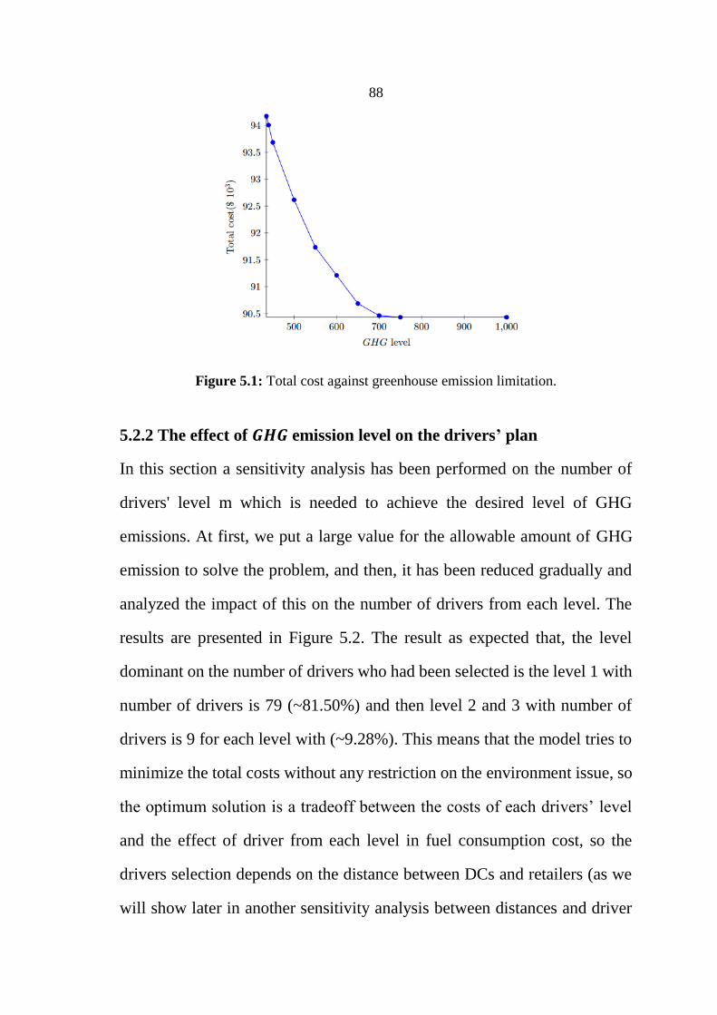
88

Figure 5.1: Total cost against greenhouse emission limitation.

5.2.2 The effect of 𝑮𝑯𝑮 emission level on the drivers’ plan

In this section a sensitivity analysis has been performed on the number of

drivers' level m which is needed to achieve the desired level of GHG

emissions. At first, we put a large value for the allowable amount of GHG

emission to solve the problem, and then, it has been reduced gradually and

analyzed the impact of this on the number of drivers from each level. The

results are presented in Figure 5.2. The result as expected that, the level

dominant on the number of drivers who had been selected is the level 1 with

number of drivers is 79 (~81.50%) and then level 2 and 3 with number of

drivers is 9 for each level with (~9.28%). This means that the model tries to

minimize the total costs without any restriction on the environment issue, so

the optimum solution is a tradeoff between the costs of each drivers’ level

and the effect of driver from each level in fuel consumption cost, so the

drivers selection depends on the distance between DCs and retailers (as we

will show later in another sensitivity analysis between distances and driver

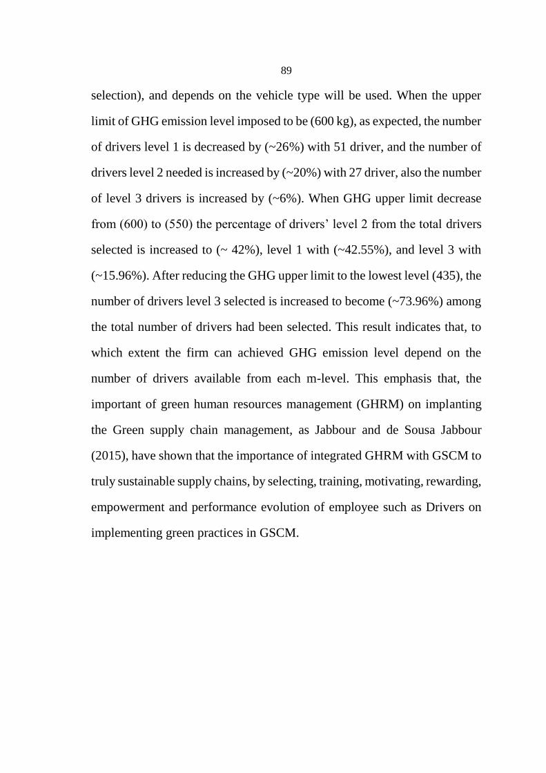
89

selection), and depends on the vehicle type will be used. When the upper

limit of GHG emission level imposed to be (600 kg), as expected, the number

of drivers level 1 is decreased by (~26%) with 51 driver, and the number of

drivers level 2 needed is increased by (~20%) with 27 driver, also the number

of level 3 drivers is increased by (~6%). When GHG upper limit decrease

from (600) to (550) the percentage of drivers’ level 2 from the total drivers

selected is increased to (~ 42%), level 1 with (~42.55%), and level 3 with

(~15.96%). After reducing the GHG upper limit to the lowest level (435), the

number of drivers level 3 selected is increased to become (~73.96%) among

the total number of drivers had been selected. This result indicates that, to

which extent the firm can achieved GHG emission level depend on the

number of drivers available from each m-level. This emphasis that, the

important of green human resources management (GHRM) on implanting

the Green supply chain management, as Jabbour and de Sousa Jabbour

(2015), have shown that the importance of integrated GHRM with GSCM to

truly sustainable supply chains, by selecting, training, motivating, rewarding,

empowerment and performance evolution of employee such as Drivers on

implementing green practices in GSCM.

90

Figure 5.2: The relation between number of m-level driver and greenhouse limitation.

5.3 Conducting a Sensitivity Analysis on the distances between DCs and

retailers

In this section sensitivity analysis will be conducted between the number of

drivers needed from each level and the distances between DCs and retailers.

After solving the problem by relaxing the GHG emission constraint, and

unification the distance between DCs and Retailers, and then increase the

distances gradually in order to analyze the distance impact on the selection

among levels of drivers as shown in Figure 5.3. As Shown in Figure 5.3,

when the distance between each DC and each retailer is less than 300 km,

the dominant number of drivers are selected from driver level 1 with

percentage equals to (~81.44%) and driver level 2 and 3 with (9.28%) for

each level. When distance increased to 500 km, the percentage of drivers’

91

level 1 selected had been reduced to (~2.08%), with increased the number of

drivers’ level 2 to (~91.67%) and drivers’ level 3 reduced to (~6.25%). And

with increasing the distance to higher than 600 km, the number of drivers’

level 3 is increased to (~97.98%), and number of drivers’ level 2 reduced to

(~2.02%) with 0.00% of drivers’ level 1. Finally, by increasing the distance

to be higher than 900 km, the number of drivers’ level 3 is increased to 100%

with 0.00% to each of drivers’ level 1 and 2. This could be due to the effect

of drivers on fuel consumption will be increased with increasing the distance.

So the model try to tradeoff between the fuel consumption saving can

achieved by driver and the cost of driver. This can indicate that the criticality

of selection drivers depend on the distance that will be assigned to drivers.

And to check the effect of vehicles’ types on selection of the drivers, we

conduct a test, which the distance between DC1 and retailer1, and the

distance between DC2 and retailer1 are equal to 1000 km, on the other hand,

the distance between DC1, DC2 with retailer 2 is equal to 50 km, the

assignments between vehicles and drivers are shown in Table 5.1. As seen

in Table 5.1, in long distances, such as between DC1 and retailer 1, most the

assignments were between vehicles of type 3 and drivers of type 3. On the

other hand, in short distance, most the assignment were between vehicles of

type 3 and drivers of type 1, other assignments are shown in Table 5.1.

92

Figure 5.3: The relation between number of m-level driver and the distance between DCs

and Retailers.

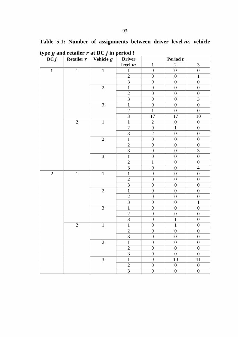
93

Table 5.1: Number of assignments between driver level 𝒎, vehicle

type 𝒈 and retailer 𝒓 at DC 𝒋 in period 𝒕 DC 𝒋 Retailer 𝒓 Vehicle 𝒈 Driver

level 𝒎

Period 𝒕

1 2 3

1 1 1 1 0 0 0

2 0 0 1

3 0 0 0

2 1 0 0 0

2 0 0 0

3 0 0 3

3 1 0 0 0

2 1 0 0

3 17 17 10

2 1 1 2 0 0

2 0 1 0

3 2 0 0

2 1 0 0 0

2 0 0 0

3 0 0 3

3 1 0 0 0

2 1 0 0

3 0 0 4

2 1 1 1 0 0 0

2 0 0 0

3 0 0 0

2 1 0 0 0

2 0 0 0

3 0 0 1

3 1 0 0 0

2 0 0 0

3 0 1 0

2 1 1 0 1 0

2 0 0 0

3 0 0 0

2 1 0 0 0

2 0 0 0

3 0 0 0

3 1 0 10 11

2 0 0 0

3 0 0 0

94

5.4 Conducting a Sensitivity Analysis on the cost of drivers

In this section, the sensitivity analysis will be conducted on the drivers' cost

such as the salaries, firing and hiring cost. Differences in costs depend on the

level of drivers. We assume that the difference in cost will be constant

between each two successive levels (i.e. the difference in cost between driver

level 1 and driver level 2 will be equal to the difference in cost between driver

level 2 and driver level 3). At the first, we put the difference in cost between

the three levels of drivers equal to zero and then the difference will be

increased step by step and the number of drivers needed from each level was

computed. The results are shown in Figures 5.4, 5.5 and 5.6.

Firstly, when the difference is equal to zero, the result as expected, the

dominant level on the number of drivers who had been selected is the level

3 with number of drivers is 73 (80.22%) and then level 2 and 3 with number

of drivers is 9 for each level with (9.89%) from the total drivers have been

selected, as shown in Figure 5.4. In specific, at DC 1 the percentage of

drivers’ level 3 who are needed is equal to 68.42% from the total drivers

needed at this DC, while the drivers’ level 1 and level 2 have a percentage

equal to 15.79%. Due to the DC 1 has an initial drivers at the beginning of

the planning horizon from level 1, level 2 and level 3. The model will be

tried to minimize the cost without violating the allowable CO2 level. In this

situation, the trade-off between firing all the drivers from level 1 and level 2

and then hiring a drivers from level 3 or maintain the drivers from level 1

and level 2 and any needed to hiring drivers should be from level 3, because

the hiring cost is equal regardless of the drivers’ level. The model conducted

95

a trade-off between the effect of drivers on fuel consumption (Transportation

variable cost) and CO2 emission and the cost of hiring and firing of drivers.

This can be a sufficient explanation of why the model did not selected all the

drivers from the level 3, these results are shown in Figure 5.5. At DC 2 all

the drivers were selected form level 3, because DC 2 in period 1 closed as

mentioned in the previous chapter (DC 2 cannot received any product from

suppliers in period 1 due to the length of the lead time), so the model laid off

all the drivers who are available at the beginning of the period 1. In period 2

and 3, the model selected all the drivers from level 3 to be hired as shown in

Figure 5.6. When the difference in cost between each two successive levels

of the drivers is equal to ($ 5), the results were as follows; the total number

of driver level 3 is decreased by 71.23% with 8 drivers, and the total number

of drivers’ level 1 is increased by 37.30% with 42 drivers, also the total

number of drivers’ level 2 is increased by 33.93% with 39 drivers.

These results can be decomposed into results related to DC1 and DC 2. In

DC 1, number of drivers’ level 1 is increased by 54.80% with 36 drivers, the

percentage of drivers level 2 is increased by 1.86% with the same number of

drivers needed that equals to 9 drivers, but the total number of drivers’ level

3 who are needed is decreased by 56.96% with 6 drivers. While at DC 2,

number of drivers’ level 1 who are selected is increased by 15.79% with 6

drivers, also the number of drivers’ level 2 is increased by 78.95%, but

number of drivers’ level 3 are decreased by 94.74% with 2 drivers. The

dominant level of drivers who are selected in DC 1 is the level 1 and in DC

2 is the level 2, this could be explained by the distance between DC 2 and

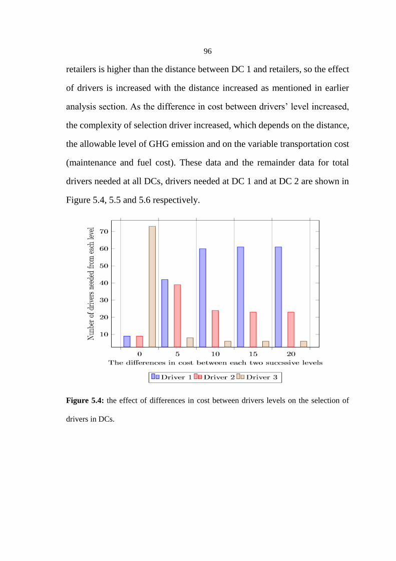
96

retailers is higher than the distance between DC 1 and retailers, so the effect

of drivers is increased with the distance increased as mentioned in earlier

analysis section. As the difference in cost between drivers’ level increased,

the complexity of selection driver increased, which depends on the distance,

the allowable level of GHG emission and on the variable transportation cost

(maintenance and fuel cost). These data and the remainder data for total

drivers needed at all DCs, drivers needed at DC 1 and at DC 2 are shown in

Figure 5.4, 5.5 and 5.6 respectively.

Figure 5.4: the effect of differences in cost between drivers levels on the selection of

drivers in DCs.

97

Figure 5.5: the effect of differences in cost between drivers levels on the selection of

drivers at DC 1.

Figure 5.6: the effect of differences in cost between drivers levels on the selection of

drivers at DC 2.

98

5.5 summary

This chapter presented the sensitivity analysis on the numerical parameters

that used in solving the proposed model. We first conduct a sensitivity

analysis on the GHG emission level and its effect on the total cost across the

supply chain. The results showed that, as the allowable GHG emission level

decreases the total cost increases. Second, we conduct a sensitivity analysis

on the GHG emission level and its effect on the selection of drivers. The

results showed that, when the GHG emission level becomes tighter, the need

to high level drivers is increased. This emphasizes on the important of drivers

in adopting the green strategies and to help organizations to comply with the

allowable GHG emission level. Third, we conduct a sensitivity analysis on

the distances between nodes in supply chain and its effect on the selection of

drivers. The results indicated that, whenever the distances become longer,

the need to high level drivers has increased. Finally, the sensitivity analysis

was conducted on the difference in cost between the levels of drivers. This

analysis was conducted with GHG emission level considers to be high

according to the presented problem (i.e. 1000, 800, and 600 Kg CO2

emission/ period), so the model tries to trade-off between the cost of drivers

and their effect on fuel consumption (Variable costs).

99

Chapter Six

Conclusions and Recommendations

100

Chapter Six

Conclusions and Recommendations

6.1 Summary

In this research, a novel approach for incorporating drivers’ differences with

aggregate production planning in a green supply chain management is

proposed. Some characteristics of the proposed model are as the following:

(1) considering the major cost parameters of supply chain such as

transportation, inventory, purchasing and human related costs; (2)

considering the green concepts in transportation issues; (3) considering

drivers’ levels in terms of green driving index (GDI) with different effect on

fuel consumption and CO2 emission, different salaries (a sort of motivation),

hiring and firing costs, and possibility of drivers’ training and upgrading; (4)

considering the types of vehicles used in transportation with different

capacities, cost, and different effect on environment; (5) considering the

assignment between drivers and vehicles.

The proposed model was formulated as mixed integer nonlinear

programming and then converted to a linear one. The model formulation and

description was presented that include the model’s assumptions, sets,

parameters, decision variables, objective function components and

constraints. And then a hypothetical numerical study was conducted and

solved using Matlab 2015a to demonstrate the validity, applicability and

solvability of the developed model. The results of this study were presented

and discussed such that the quantities to be shipped from suppliers to DCs

101

and from DCs to retailers, the workforce plan for workers and drivers,

number and type of vehicles should be used, the assignment between drivers,

vehicles and then to the destinations (retail stores). In addition, the

sensitivity analysis was conducted on the GHG emissions level, the distances

between DCs and retailers, and the differences in cost between drivers. The

results of conducting sensitivity analysis demonstrate that, after considering

green issues (reducing the allowable GHG emissions level) the total cost

across the supply chain was increased. And the number of drivers for each

level varies with different GHG emission level, so the CO2 emission level

that the company wants to achieve depends on the level of drivers' available.

Also the assignments between vehicles and drivers varies with different

GHG emission level and different distances.

The results of this study are important in a number of aspects. Foremost

among these, the proposed model in this thesis conducted numerous

assignment matrices to ensure that each driver will be assigned to one vehicle

and one retail store, and each vehicle will be assigned to one driver and one

retail store. So the effect of each combination between vehicles and drivers

on fuel consumption and CO2 emissions will be computed by taking into

account the distances. So the proposed model will try to conduct an optimally

assigning between vehicles, drivers and the destination (i.e. retail stores) to

reduce the CO2 emission, fuel consumption and the total shipping cost across

the supply chain with taking into account the differences impact of drivers

and vehicles on CO2 emission and fuel consumption as well as on the total

cost.

102

6.2 Contribution

This research contributes to the literature with a more realistic model that

takes drives selecting, training, motivating and assigning to vehicles into

account in managing and planning supply chain at tactical and operational

levels. In contrast to previous researches that have completely ignored the

differences between drivers in design and managing GSC. This approach

allow us to address integrating drivers’ differences (in term of GDI) to

determine the best scenario for selecting, training and assigning drivers to

fulfill a company’s aims for reducing their fuel consumption and CO2

emission in their supply chains. The results showed that the level of carbon

dioxide emissions that the company's willing to achieve depends heavily on

the level of available drivers have and on how to select, train and assign those

drivers. Therefore, this research provides decision-makers with more

realistic model. This model will support the company’s management with a

sufficient knowledge about how to achieve a desired level of CO2 emission

by considering drivers’, vehicles’, and distances’ effect, and on the other

hand minimizing the total cost incurred across the supply chain.

Implementing green supply chain is a human responsibility and without

considering human aspects the truly implementing of GSCM cannot be

achieved.

6.3 Limitations and Future Recommendations

In spite of the model’s strengths, the proposed model has a number of

limitations that can make the results unrealistic. These limitations and the

proposed recommendations can be described as follows:

103

Although the model gives logical results, it is relied on hypothetical

data represents the researchers’ experience in addition to data derived

from the related literature, such that the drivers’ performance

parameters. Evaluating drivers’ performance based on fairly

performance evaluation methodology such as the methodology that

developed by Liimatainen (2011) he integrated incentive system based

on fairly performance evaluation of the drivers. Also, integrating

qualitative method such as AHP, fuzzy logic and Technique for Order

of Preference by Similarity to Ideal Solution (TOPSIS) in selecting

drivers based on green criteria (i.e. experiences, Eco-driving training,

ages, personalities, awareness and education; may be each driver has

a profile include the average of fuel consumption per km) may give

more realistic output.

All parameters in the developed model are assumed to be deterministic

and known such as that all cost parameters, lead time and drivers’

performance. Solving the model using stochastic approach may give a

more robust results.

6.4 Future Works

It is evident that the research of GSCM did not reach the end, and the

opportunity is still exist to develop the proposed model to become more

comprehensive and realistic. The proposals for future research can be

described as follows:

104

Implementing the proposed model by using real cases which is one of

the promoting future work, to demonstrate the importance of

integrating drivers’ differences in improving the supply chain’s

ecological and economic performance.

Integrating other factors that may affect fuel consumption and CO2

emission such as vehicles weight with considering weight of the

products and route selection by modeling the relation between

vehicle’s weight or route condition, fuel consumption and CO2

emission are promising areas for future research.

Considering other gases emission such as CO, NOx, etc.

Integrating other green issues in GSC optimization model such as

green design (designing the product based on its environmental impact

by integrating Life Cycle assessment (LCA) of the products).

Integrating other human aspects such as the effect of human factors in

the process of designing and producing the green products. And

demonstrate the need to green training and selection of the employees.

105

References

- Abdallah, T., Diabat, A., and Simchi-Levi, D. (2010). A carbon sensitive

supply chain network problem with green procurement. In: 2010 40th

International Conference on Computers and Industrial Engineering

(CIE), IEEE, pp. 1-6.

- Alam, M. S., and McNabola, A. (2014). A critical review and assessment

of Eco-Driving policy & technology: Benefits & limitations. Transport

Policy, 35, 42-49.

- Alessandrini, A., Orecchini, F., Ortenzi, F., and Campbell, F. V. (2009).

Drive-style emissions testing on the latest two Honda hybrid

technologies. European Transport Research Review, 1(2), 57-66.

- Barbosa-Póvoa, A. P. (2009). Sustainable supply chains: key

challenges. Computer Aided Chemical Engineering, 27, 127-132.

- Barkenbus, J. N. (2010). Eco-driving: An overlooked climate change

initiative. Energy Policy, 38(2), 762-769.

- Baykasoglu, A. (2001). MOAPPS 1.0: aggregate production planning

using the multiple-objective tabu search. International Journal of

Production Research, 39(16), 3685-3702.

- Beamon, B.M. (1999). Designing the green supply chain. Logistics

Information Management, 12, 332–342.

- Bloemhof-Ruwaard, J. M., Van Wassenhove, L. N., Gabel, H. L., and

Weaver, P. M. (1996). An environmental life cycle optimization model

for the European pulp and paper industry. Omega, 24(6), 615-629.

106

- Boriboonsomsin, K., and Barth, M. (2009). Impacts of road grade on

fuel consumption and carbon dioxide emissions evidenced by use of

advanced navigation systems. Transportation Research Record:

Journal of the Transportation Research Board, (2139), 21-30.

- Bradshaw, C. J., Bowman, D. M., Bond, N. R., Murphy, B. P., Moore, A.

D., Fordham, D. A. and Dalal, R. C. (2013). Brave new green world–

consequences of a carbon economy for the conservation of Australian

biodiversity. Biological Conservation, 161, 71-90.

- Bussieck, M. R., and Pruessner, A. (2003). Mixed-integer nonlinear

programming. SIAG/OPT Newsletter: Views & News, 14(1), 19-22.

- Billatos, S. (1997). Green technology and design for the environment.

CRC Press.

- Cachon, G. P. (1999). Competitive supply chain inventory management.

In Quantitative models for supply chain management (pp. 111-146).

Springer US.

- Carrese, S., Gemma, A., and La Spada, S. (2013). Impacts of driving

behaviors, slope and vehicle load factor on bus fuel consumption and

emissions: a real case study in the city of Rome. Procedia-Social and

Behavioral Sciences, 87, 211-221.

- Chiou, T. Y., Chan, H. K., Lettice, F., and Chung, S. H. (2011). The

influence of greening the suppliers and green innovation on

environmental performance and competitive advantage in

Taiwan. Transportation Research Part E: Logistics and

Transportation Review, 47(6), 822-836.

107

- Chopra, S., and Meindl, P. (2013). Supply chain management: strategy,

planning, and operation (global Ed.). Boston [etc.: Pearson.

- Chouinard, M., D’Amours, S., and Aït-Kadi, D. (2005). Integration of

reverse logistics activities within a supply chain information

system. Computers in Industry, 56(1), 105-124.

- Coskun, S., Ozgur, L., Polat, O., and Gungor, A. (2016). A model

proposal for green supply chain network design based on consumer

segmentation. Journal of Cleaner Production, 110, 149-157.

- CSCMP (Council of Supply Chain Management Professionals). (2016,

March 13). Retrieved from https://cscmp.org/supply-chain-management-

definitions.

- Daily, B. F., and Huang, S. C. (2001). Achieving sustainability through

attention to human resource factors in environmental

management. International Journal of Operations & Production

Management, 21(12), 1539-1552.

- Daily, B. F., Bishop, J. W., and Massoud, J. A. (2012). The role of

training and empowerment in environmental performance: A study of

the Mexican maquiladora industry. International Journal of

Operations & Production Management, 32(5), 631-647.

- Daily, B. F., Bishop, J. W., and Steiner, R. (2011). The mediating role of

EMS teamwork as it pertains to HR factors and perceived

environmental performance. Journal of Applied Business Research

(JABR), 23(1).

108

- Dawei, Z., Hamid, A. B. A., Chin, T. A., and Leng, K. C. (2015). Green

Supply Chain Management: A Literature Review. Sains

Humanika, 5(2), 15-21.

- DeCicco, J., and Ross, M. (1996). Recent advances in automotive

technology and the cost-effectiveness of fuel economy

improvement. Transportation Research Part D: Transport and

Environment, 1(2), 79-96.

- Dekker, R., Bloemhof, J., and Mallidis, I. (2012). Operations Research

for green logistics–An overview of aspects, issues, contributions and

challenges. European Journal of Operational Research, 219(3), 671-

679.

- Diabat, A., and Simchi-Levi, D. (2009, December). A carbon-capped

supply chain network problem. In Industrial Engineering and

Engineering Management, 2009. IEEM 2009. IEEE International

Conference on (pp. 523-527). IEEE.

- Dornfeld, D., Yuan, C., Diaz, N., Zhang, T., and Vijayaraghavan, A. (2013).

Introduction to green manufacturing. In Green Manufacturing (pp.1-23)

Springer US.

- Duber-Smith, D. C. (2005), ―The green imperative, Soap, Perfumery,

and Cosmetics,

- Edmunds (2005). We test the tips. What really save gas? And how

much? Retrieved from :< http://www.edmunds.com/fuel-economy/we-

test-the-tips.html> [Accessed date: 13 March 2016]

109

- Elhedhli, S., and Merrick, R. (2012). Green supply chain network design

to reduce carbon emissions. Transportation Research Part D:

Transport and Environment, 17(5), 370-379.

- EPA, (2011a). EPA Fuel economy guide, 2011. Retrieved Form: <

https://www.fueleconomy.gov/feg/FEG2011.pdf>. [Accessed date: 5

March 2016]

- EPA, (2011b). Gas mileage tips- keeping your car in shape, 2011.

Available at: < https://www.fueleconomy.gov/feg/maintain.jsp >.

[Accessed date: 5 March 2016]

- EPA, (2011c). Gas mileage tips- keeping your car efficiently, 2011.

Available at: < https://www.fueleconomy.gov/feg/driveHabits.jsp >.

[Accessed date: 5 March 2016]

- EPA, (2011d). Many factors affect MPG, 2011. Available at: <

https://www.fueleconomy.gov/feg/factors.shtml >.

- Ericsson, E. (2001). Independent driving pattern factors and their

influence on fuel-use and exhaust emission factors. Transportation

Research Part D: Transport and Environment, 6(5), 325-345.

- Facanha, C. (2009). Effects of congestion and road level of service on

vehicle fuel economy. In Transportation Research Board 88th

Annual Meeting (No. 09-0268).

- Fahimnia, B., Farahani, R. Z., Marian, R., and Luong, L. (2013). A review

and critique on integrated production–distribution planning models

and techniques. Journal of Manufacturing Systems, 32(1), 1-19.

110

- Fahimnia, B., Sarkis, J., and Eshragh, A. (2015). A tradeoff model for

green supply chain planning: A leanness-versus-greenness

analysis. Omega, 54, 173-190.

- Gilbert, S. (2001). Greening supply chain: Enhancing competitiveness

through green productivity. Tapei, Taiwan, 16.

- Gottberg, A., Morris, J., Pollard, S., Mark-Herbert, C., and Cook, M.

(2006). Producer responsibility, waste minimisation and the WEEE

Directive: Case studies in eco-design from the European lighting

sector. Science of the Total Environment, 359(1), 38-56.

- Govindarajulu, N., and Daily, B. F. (2004). Motivating employees for

environmental improvement. Industrial Management & Data

Systems, 104(4), 364-372.

- Grant, A. J., and Campbell, G. G. (1994). The meaning of environmental

values for managers. Environmental Quality Management, 3(4), 507-

512.

- Graves, L. M., Sarkis, J., and Zhu, Q. (2013). How transformational

leadership and employee motivation combine to predict employee

proenvironmental behaviors in China. Journal of Environmental

Psychology, 35, 81-91.

- Govindan, K., Diabat, A., and Shankar, K. M. (2015). Analyzing the

drivers of green manufacturing with fuzzy approach. Journal of

Cleaner Production, 96, 182-193.

111

- Grossmann, I. E. (2004). Challenges in the new millennium: product

discovery and design, enterprise and supply chain optimization, global life

cycle assessment. Computers & Chemical Engineering, 29(1), 29-39.

- Giusti, L. (2009). A review of waste management practices and their

impact on human health. Waste management, 29(8), 2227-2239.

- Haehling LC. (1970). Production and employment scheduling in

multistage production systems. Naval Research Logistics Quarterly,

17(2), 193-198.

- Hanssman, F., and Hess, S. W. (1960). A linear programming approach

to production and employment scheduling. Management science, (1),

46-51.

- Hervani, A. A., Helms, M. M., and Sarkis, J. (2005). Performance

measurement for green supply chain management. Benchmarking: An

international journal, 12(4), 330-353.

- Hugo, A., and Pistikopoulos, E. N. (2005). Environmentally conscious

long-range planning and design of supply chain networks. Journal of

Cleaner Production, 13 (15), 1471-1491.

- Hugos, M. H. (2011). Essentials of supply chain management, 3ed

edition. John Wiley & Sons.

- Jabbour, C. J. C., and de Sousa Jabbour, A. B. L. (2015). Green human

resource management and green supply chain management: Linking two

emerging agendas. Journal of Cleaner Production, 112, 1824-1833.

- Jabbour, C. J. C., and Santos, F. C. A. (2008). Relationships between

human resource dimensions and environmental management in

112

companies: proposal of a model. Journal of Cleaner Production, 16(1),

51-58.

- Jabbour, C. J. C., Santos, F. C. A., Fonseca, S. A., and Nagano, M. S.

(2013). Green teams: understanding their roles in the environmental

management of companies located in Brazil. Journal of Cleaner

Production, 46, 58-66.

- Jamshidi, R., Ghomi, S. F., and Karimi, B. (2012). Multi-objective green

supply chain optimization with a new hybrid memetic algorithm using

the Taguchi method. Scientia Iranica, 19(6), 1876-1886.

- Jofre, S., and Morioka, T. (2005). Waste management of electric and

electronic equipment: comparative analysis of end-of-life

strategies. Journal of Material Cycles and Waste Management, 7(1),

24-32.

- Kaiser, B., Eagan, P. D., and Shaner, H. (2001). Solutions to health care

waste: life-cycle thinking and" green" purchasing. Environmental

Health Perspectives, 109(3), 205.

- Kannan, D., Khodaverdi, R., Olfat, L., Jafarian, A., and Diabat, A. (2013).

Integrated fuzzy multi criteria decision making method and multi-

objective programming approach for supplier selection and order

allocation in a green supply chain. Journal of Cleaner Production, 47,

355-367.

- Kopicki, R.J., Legg, L., Berg, L.M.J., Dasappa, V. and Maggioni, C. (eds)

(1993). Reuse and Recycling: Reverse Logistics Opportunities. Oak

Brook, IL: Council of Logistics Management.

113

- Kurani, K., Sanguinetti, A., and Park, H. (2015). “Actual Results May

Vary”: A Behavioral Review of Eco-‐Driving for Policy Makers. White

Paper, National Center for Sustainable Transportation, University of

California at Davis, Davis, CA, July.

- Lai, W. T. (2015). The effects of eco-driving motivation, knowledge and

reward intervention on fuel efficiency. Transportation research part

D: transport and environment, 34, 155-160.

- Larsen-Skjott, T., Schary, P. B., Mikkola, J. H., and Kotzab, H. (2007).

Managing the Global Supply Chain. Copenhagen: Copenhagen

Business School Press/Liber.

- Lash, J., and Willington, F. (2007). Competitive Advantage on a

Warming Planet. Harvard Business Review, 1-11.

- LeBlanc, D. J., Sivak, M., and Bogard, S. (2010). Using naturalistic

driving data to assess variations in fuel efficiency among individual

drivers.

- Lee, S. Y. (2008). Drivers for the participation of small and medium-

sized suppliers in green supply chain initiatives. Supply Chain

Management: An International Journal, 13(3), 185-198.

- Levi, D. S., Kaminsky, P., and Levi, E. S. (2003). Designing and

managing the supply chain: Concepts, strategies, and case studies. New

York, NY, USA: McGraw-Hill.

- Liang, Z. and Chaovalitwongse, W. A. and Shi, L. (2016). Supply Chain

Management and Logistics: Innovative Strategies and Practical

Solutions. Taylor & Francis Group.

114

- Liimatainen, H. (2011). Utilization of fuel consumption data in an Eco

driving incentive system for heavy-duty vehicle drivers. Intelligent

Transportation Systems, IEEE Transactions on, 12(4), 1087-1095.

- Liu, S., and Papageorgiou, L. G. (2013). Multi objective optimisation of

production, distribution and capacity planning of global supply chains

in the process industry. Omega, 41(2), 369-382.

- Li, K., Zhang, X., Leung, J. Y. T., and Yang, S. L. (2016). Parallel

machine scheduling problems in green manufacturing

industry. Journal of Manufacturing Systems, 38, 98-106.

- Mann, M. K., Spath, P. L., and Craig, K. R. (1996). Economic and life

cycle assessment of an integrated biomass gasification combined cycle

system. In Energy Conversion Engineering Conference, 1996. IECEC

96., Proceedings of the 31st Intersociety (Vol. 3, pp. 2134-2139). IEEE.

- Martin, E., Chan, N., and Shaheen, S. (2012). How public education on

eco-driving can reduce both fuel use and greenhouse gas emissions.

Transportation Research Record: Journal of the Transportation

Research Board, (2287), 163-173.

- Martinsen, U., and Huge-Brodin, M. (2010). Greening the offerings of

logistics service providers. In The 22nd Annual NOFOMA

Conference, June 10-11, Kolding, Denmark (pp. 969-984).

- Masud, A. S., and Hwang, C. L. (1980). An aggregate production

planning model and application of three multiple objective decision

methods. International Journal of Production Research, 18(6), 741-

752.

115

- Memari, A., Rahim, A. R. A., and Ahmad, R. B. (2015). An Integrated

Production-distribution Planning in Green Supply Chain: A Multi-

objective Evolutionary Approach. Procedia CIRP, 26, 700-705.

- Mentzer, J. T., DeWitt, W., Keebler, J. S., Min, S., Nix, N. W., Smith, C.

D.,and Zacharia, Z. G.(2001).Defining supply chain management. Journal

of Business logistics, 22(2), 1-25.

- Min, H., and Galle, W. P. (2001). Green purchasing practices of US

firms. International Journal of Operations & Production

Management, 21(9), 1222-1238.

- Min, H., and Zhou, G. (2002). Supply chain modeling: past, present and

future. Computers & industrial engineering, 43(1), 231-249.

- Melnyk, S. A., and Smith, R. T. (1996). Green Manufacturing, Society

for Manufacturing Engineering. Dearborn, MI.

- Mirzapour Al-e-hashem, S. M. J., Baboli, A., and Sazvar, Z. (2013). A

stochastic aggregate production planning model in a green supply

chain: Considering flexible lead times, nonlinear purchase and

shortage cost functions. European Journal of Operational

Research, 230(1), 26-41.

- Mirzapour Al-e-hashem, S. M. J., Baboli, A., Aryanezhad, M. B., and

Sazvar, Z., (2011b). Aggregate production planning in a green supply

chain by considering flexible lead times and multi breakpoint purchase

and shortage cost functions. In 41st International conference on

computers & Industrials Engineering. Los Angeles, CA USA.

116

- Mirzapour Al-e-hashem, S. M. J., Baboli, A., Aryanezhad, M. B., and

Sazvar, Z. (2011a). Aggregate production planning in a green supply

chain by considering flexible lead times and multi breakpoint purchase

and shortage cost functions. In: 41st International Conference on

Computers & Industrial Engineering. Los Angeles, CA USA.

- Natural Resources Canada (2009). 2007 Vehicle Survey, Summary

Report. Office of Energy Publications, Ottawa, Canada.

- Neto, J. Q. F., Bloemhof-Ruwaard, J. M., van Nunen, J. A., and van Heck,

E. (2008). Designing and evaluating sustainable logistics

networks. International Journal of Production Economics, 111(2),

195-208.

- Ninlawan, C., Seksan, P., Tossapol, K., and Pilada, W. (2010). The

implementation of green supply chain management practices in

electronics industry. In Proceedings of the international multi

conference of engineers and computer scientists (Vol. 3, pp. 17-19).

- Nylund, N. O. (2006). Fuel savings for heavy-duty vehicles

‘HDEnergy’. Summary report 2003-2005. Project Report VTT.

- Paiva, R. P., and Morabito, R. (2009). An optimization model for the

aggregate production planning of a Brazilian sugar and ethanol milling

company. Annals of Operations Research, 169(1), 117-130.

- Paksoy, T., Bektaş, T., and Özceylan, E. (2011). Operational and

environmental performance measures in a multi-product closed-loop

supply chain. Transportation Research Part E: Logistics and

Transportation Review, 47(4), 532-546.

117

- Paksoy, T., O¨ zceylan, E., Weber, G. W., Barsoum, N., Weber, G. W.,

and Vasant, P. (2010). A multi objective model for optimization of a

green supply chain network. In AIP Conference Proceedings (Vol.

1239, No. 1, p. 311).

- Pishvaee, M. S., and Razmi, J. (2012). Environmental supply chain

network design using multi-objective fuzzy mathematical

programming. Applied Mathematical Modelling, 36(8), 3433-3446.

- Porter, M. E., and Van der Linde, C. (1995). Toward a new conception

of the environment- competitiveness relationship. The journal of

economic perspectives, 9(4), 97-118.

- Ramezanian, R., Rahmani, D., and Barzinpour, F. (2012). An aggregate

production planning model for two phase production systems: Solving

with genetic algorithm and tabu search. Expert Systems with

Applications, 39(1), 1256-1263.

- Ramudhin, A., Chaabane, A., Kharoune, M., and Paquet, M. (2008).

Carbon market sensitive green supply chain network design.

In Industrial Engineering and Engineering Management, 2008.

IEEM 2008. IEEE International Conference on (pp. 1093-1097).

IEEE.

- Rettab, B., and Ben Brik, A. (2008). Green supply chain in

Dubai. Dubai, UAE: Dubai Chamber Centre for Responsible

Business.

- Rodrigue, P. and Slack, B. and Comtois C. (2011). Green Logistics,

retrieved from:

118

http://people.hofstra.edu/geotrans/eng/ch8en/appl8en/ch8a4en.html on

March 3, 2016.

- Rose, C. M., Beiter, K. A., and Ishii, K. (1999). Determining end-of-life

strategies as a part of product definition. In Electronics and the

Environment, 1999. ISEE-1999. Proceedings of the 1999 IEEE

International Symposium on (pp. 219-224). IEEE.

- Sanders, N. R. (2011). Supply chain management: A global

perspective. Wiley Global Education.

- Sarkis, J. (2003). A strategic decision framework for green supply chain

management. Journal of cleaner production, 11(4), 397-409.

- Sarkis, J., Gonzalez-Torre, P., and Adenso-Diaz, B. (2010). Stakeholder

pressure and the adoption of environmental practices: The mediating

effect of training. Journal of Operations Management, 28(2), 163-176.

- Shapiro, J.F., (2004). Optimization Models of Supply Chain

Management; CLM Explores. Council of Logistic Management, Oak

Book, II.

- Sillekens, T., Koberstein, A., and Suhl, L. (2011). Aggregate production

planning in the automotive industry with special consideration of

workforce flexibility. International Journal of Production Research,

49(17), 5055-5078.

- Simchi-Levi, D., Chen, X., and Bramel, J. (2013). The logic of logistics:

theory, algorithms, and applications for logistics management. 3rd

Edition. Springer Science & Business Media.

119

- Simões M, Carvalho A, de Freitas CL, and Barbosa-Póvoa AP (2014).

How to assess social aspects in supply chains? Proceedings 8th

International Conference Found Comput-Aided Process Des –

FOCAPD, 801-6.

- Sinding, K. (2000). Environmental management beyond the boundaries

of the firm: definitions and constraints. Business strategy and the

environment, 9(2), 79.

- Sivak, M., and Schoettle, B. (2012). Eco-driving: Strategic, tactical, and

operational decisions of the driver that influence vehicle fuel economy.

Transport Policy, 22, 96-99.

- Srivastava, S. K., and Srivastava, R. K. (2006). Managing product

returns for reverse logistics. International Journal of Physical

Distribution & Logistics Management, 36(7), 524-546.

- Srivastava, S.K. (2007). Green supply-chain management: a state-of-

the-art literature review. International journal of management

reviews, 9(1), 53-80.

- Stillwater, T., and Kurani, K. S. (2013). Drivers discuss eco-driving

feedback: Goal setting, framing, and anchoring motivate new

behaviors. Transportation research part F: traffic psychology and

behaviour, 19, 85-96.

- Sharma, S. (2000). Managerial interpretations and organizational

context as predictors of corporate choice of environmental

strategy. Academy of Management journal, 43(4), 681-697.

120

- Sundarakani, B., De Souza, R., Goh, M., Wagner, S. M., and

Manikandan, S. (2010). Modeling carbon footprints across the supply

chain. International Journal of Production Economics, 128(1), 43-50.

- Talaei, M., Moghaddam, B. F., Pishvaee, M. S., Bozorgi-Amiri, A., and

Gholamnejad, S. (2015). A robust fuzzy optimization model for carbon-

efficient closed-loop supply chain network design problem: a numerical

illustration in electronics industry. Journal of Cleaner Production,

113, 662-673.

- Tang, T. Q., Huang, H. J., and Shang, H. Y. (2015). Influences of the

driver’s bounded rationality on micro driving behavior, fuel

consumption and emissions. Transportation Research Part D:

Transport and Environment, 41, 423-432.

- Testa, F., and Iraldo, F. (2010). Shadows and lights of GSCM (Green

Supply Chain Management): determinants and effects of these

practices based on a multi-national study. Journal of Cleaner

Production, 18(10), 953-962.

- Theyel, G. (2006). Customer and supplier relations for environmental

performance. In Greening the supply chain (pp. 139-149). Springer

London.

- Tognetti, A., Grosse-Ruyken, P. T., and Wagner, S. M. (2015). Green

supply chain network optimization and the trade-off between

environmental and economic objectives. International Journal of

Production Economics, 170, 385-392.

121

- TRB (Transportation Research Board), (2000). Highway capacity

manual 2000. National Academy of Science, Washington, D.C.

- Tsai, W. H., and Hung, S. J. (2009). A fuzzy goal programming approach

for green supply chain optimisation under activity-based costing and

performance evaluation with a value-chain structure. International

Journal of Production Research, 47(18), 4991-5017.

- Vagg, C., Brace, C. J., Hari, D., Akehurst, S., Poxon, J., and Ash, L.

(2013). Development and field trial of a driver assistance system to

encourage eco-driving in light commercial vehicle fleets. Intelligent

Transportation Systems, IEEE Transactions on, 14(2), 796-805.

- Van der Voort, M., Dougherty, M. S., and van Maarseveen, M. (2001). A

prototype fuel-efficiency support tool. Transportation Research Part

C: Emerging Technologies, 9(4), 279-296.

- Van Hoek, R. I. (1999). From reversed logistics to green supply

chains. Supply Chain Management: An International Journal, 4(3),

129-135.

- Vangi, D., and Virga, A. (2003). Evaluation of energy-saving driving

styles for bus drivers. Proceedings of the Institution of Mechanical

Engineers, Part D: Journal of Automobile Engineering, 217(4), 299-

305.

- Venkat, K., and Wakeland, W. (2006). Is lean necessarily green?. In

Proceedings of the 50th Annual Meeting of the ISSS-2006, Sonoma,

CA, USA.

122

- Wang, F., Lai, X., and Shi, N. (2011). A multi-objective optimization for

green supply chain network design. Decision Support Systems, 51(2),

262-269.

- Wisner, J., Tan, K. C., and Leong, G. (2015). Principles of supply chain

management: a balanced approach. Cengage Learning.

- Wu, H. J., and Dunn, S. C. (1995). Environmentally responsible logistics

systems. International Journal of Physical Distribution & Logistics

Management, 25(2), 20-38.

- Wu, Z., and Pagell, M. (2011). Balancing priorities: Decision-making

in sustainable supply chain management. Journal of Operations

Management, 29(6), 577-590.

- Yang, C. S., Lu, C. S., Haider, J. J., and Marlow, P. B. (2013). The effect

of green supply chain management on green performance and firm

competitiveness in the context of container shipping in

Taiwan. Transportation Research Part E: Logistics and

Transportation Review, 55, 55-73.

- Yeh, W. C., and Chuang, M. C. (2011). Using multi-objective genetic

algorithm for partner selection in green supply chain problems. Expert

Systems with Applications, 38(4), 4244-4253.

- You, F., and Grossmann, I. E. (2008). Mixed-integer nonlinear

programming models and algorithms for large-scale supply chain

design with stochastic inventory management. Industrial &

Engineering Chemistry Research, 47(20), 7802-7817.

123

- Young, M. S., Birrell, S. A., and Stanton, N. A. (2011). Safe driving in a

green world: A review of driver performance benchmarks and

technologies to support ‘smart’ driving. Applied ergonomics, 42(4),

533-539.

- Yue, D., Slivinsky, M., Sumpter, J., and You, F. (2014). Sustainable

design and operation of cellulosic bioelectricity supply chain networks

with life cycle economic, environmental, and social optimization.

Industrial & Engineering Chemistry Research, 53(10), 4008-4029.

- Zarkadoula, M., Zoidis, G., and Tritopoulou, E. (2007). Training urban

bus drivers to promote smart driving: A note on a Greek eco-driving

pilot program. Transportation Research Part D: Transport and

Environment, 12(6), 449-451.

- Zhu, Q., and Geng, Y. (2001). Integrating environmental issues into

supplier selection and management. Greener Management

International, 2001(35), 26-40.

- Zhu, Q., and Sarkis, J. (2004). Relationships between operational

practices and performance among early adopters of green supply chain

management practices in Chinese manufacturing enterprises. Journal

of operations management, 22(3), 265-289.

- Zhu, Q., Sarkis, J., and Geng, Y. (2005). Green supply chain management

in China: pressures, practices and performance. International Journal of

Operations & Production Management, 25(5), 449-468.

124

- Zhu, Q., Sarkis, J., and Lai, K. H. (2008a). Green supply chain

management implications for “closing the loop”. Transportation

Research Part E: Logistics and Transportation Review, 44(1), 1-18.

- Zhu, Q., Sarkis, J., and Lai, K. H. (2008b). Confirmation of a measurement

model for green supply chain management practices

implementation. International journal of production economics, 111(2),

261-273.

- Zhu, Q., Sarkis, J., and Lai, K. H. (2012). Examining the effects of green

supply chain management practices and their mediations on

performance improvements. International journal of production

research, 50(5), 1377-1394.

- Zsidisin, G. A., and Siferd, S. P. (2001). Environmental purchasing: a

framework for theory development. European Journal of Purchasing

& Supply Management, 7(1), 61-73.

جامعة النجاح الوطنية

اسات العليا كلية الدر

نماذج الأمثلة في أدارة سلاسل الأمداد الخضراء

اعداد عيسى عسراوي

اشراف د. يحيى صالح د. محمد عثمان

قدمت هذه الأطروحة أستكمالا لمتطلبات الحصول على درجة الماجتسير في الادارة الهندسية بكلية نابلس، فلسطينالدراسات العليا في جامعة النجاح الوطنية في

2016

ب

نماذج الامثلة في ادراة سلاسل الامداد الخضراء اعداد

عيسى عسراوي اشراف

د. يحيى صالح د. محمد عثمان

الملخصلقد حظيت سلاسل الامداد الخضراء على اهتمام كبير من الباحثين في العقود القليلة الماضية، ولكن

ميم وأدارة السلاسل الخضراء. في هذا البحث، نحن نطور تم تجاهل تأثير العوامل البشرية في تصنهجا جديدا لدمج اختلافات السائقين لدراسة تأثيرهم على استهلاك الوقود وانبعاثات ثاني اكسيد

التكتيكي و التشغيلي. و بشكل اكثر تحديدا، الكربون في امثلة سلاسل الامداد الخضراء على المستوى تم اقتراح نموذج برمجي غير خطي مختلط من المتغيرات الصحيحة وغير الصحيحة ليتعامل مع

مع مراعاة اختلاف المستويات بين السائقين و اختلاف انواع المركبات. تخطيط الانتاج التجميعيغاز ثاني اكسيد الكربون عبر سلسلة التوريد. يهدف النموذج لتقليل التكلفة الكلية و انبعاثات

الأمثل بين السائقين والمركبات و الوجهات، بالاضافة الى ذلك، يهدف النموذج لاستنباط التعيينفضلا عن الاختيار و التدريب الامثل للسائقين. تم اجراء دراسة عددية للتأكد من صلاحية النموذج

هرت نتائج تحليل الحساسيه،أنه وبعد أعتبار القضايا الخضراء فأن المقترح و قابليتيه للتطبيق. و أظالتكلفة الاجمالية عبر سلسلة التوريد تزداد. و عدد السائقين المطلوبين من كل مستوى يختلف باختلاف مستوى ثاني اكسيد الكربون المسموح به. لذلك فان مستوى انبعاثات ثاني أكسيد الكربون

قيقه يعتمد على مستوى السائقين المتوفر لديها. وكذلك التعيينات بين السائقين التي تسعى الشركات لتح والمركبات تختلف باختلاف مستوى ثاني اكسيد الكربون واختلاف المسافات بين مرافق سلسة الامداد.