Optimization in Machine Learning - University of Wisconsinâ€“Madison

Optimization in Machine LearningRecent Developments and Current Challenges

Stephen Wright

University of Wisconsin-Madison

NIPS Workshop, Whistler, 12 December 2008

Stephen Wright (UW-Madison) Optimization in Machine LearningNIPS Workshop, Whistler, 12 December 2008 1

/ 49

Summary

1 Sparse / Regularized Optimization

2 SVM Formulations

3 SVM Algorithms (recently proposed)

4 New optimization tools of possible interest.


/ 49

Themes

Optimization problems from machine learning are difficult (size, kerneldensity, ill conditioning)

Machine learning community has made excellent use of optimizationtechnology. Many interesting adaptations of fundamental algorithmsthat exploit the structure and fit the requirements of the application.

Several current topics in optimization may be of interest in solvingmachine learning problems.


/ 49

Sparse Optimization

Traditionally, research on algorithmic optimization assumes exact dataavailable and precise solutions needed.

However, in many optimization applications we prefer simple, approximatesolutions to more complicated exact solutions.

simple solutions easier to actuate;

uncertain data does not justify precise solutions; regularized solutionsless sensitive to inaccuracies;

simple solution more “generalizable.”

These new “ground rules” may change the algorithmic approach altogther.

For example, an approximate first-order method applied to a nonsmoothformulation may be preferred to a second-order method applied to asmooth formulation.


/ 49

Regularized Formulations

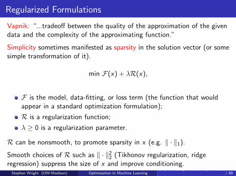
Vapnik: “...tradeoff between the quality of the approximation of the givendata and the complexity of the approximating function.”

Simplicity sometimes manifested as sparsity in the solution vector (or somesimple transformation of it).

min F(x) + λR(x),

F is the model, data-fitting, or loss term (the function that wouldappear in a standard optimization formulation);

R is a regularization function;

λ ≥ 0 is a regularization parameter.

R can be nonsmooth, to promote sparsity in x (e.g. ‖ · ‖1).

Smooth choices of R such as ‖ · ‖22 (Tikhonov regularization, ridgeregression) suppress the size of x and improve conditioning.


/ 49

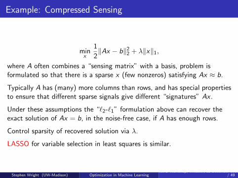
Example: Compressed Sensing

minx

1

2‖Ax − b‖22 + λ‖x‖1,

where A often combines a “sensing matrix” with a basis, problem isformulated so that there is a sparse x (few nonzeros) satisfying Ax ≈ b.

Typically A has (many) more columns than rows, and has special propertiesto ensure that different sparse signals give different “signatures” Ax .

Under these assumptions the “`2-`1” formulation above can recover theexact solution of Ax = b, in the noise-free case, if A has enough rows.

Control sparsity of recovered solution via λ.

LASSO for variable selection in least squares is similar.


/ 49

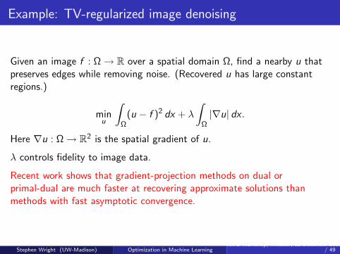
Example: TV-regularized image denoising

Given an image f : Ω→ R over a spatial domain Ω, find a nearby u thatpreserves edges while removing noise. (Recovered u has large constantregions.)

minu

∫Ω(u − f )2 dx + λ

∫Ω|∇u| dx .

Here ∇u : Ω→ R2 is the spatial gradient of u.

λ controls fidelity to image data.

Recent work shows that gradient-projection methods on dual orprimal-dual are much faster at recovering approximate solutions thanmethods with fast asymptotic convergence.


/ 49

Example: Cancer Radiotherapy

In radiation treatment planning, there are an astronomical variety ofpossibilies for delivering radiation from a device to a treatment area. Canvary beam shape, exposure time (weight), angle.

Aim to deliver a prescribed radiation dose to the tumor while avoidingsurrounding critical organs and normal tissue. Also wish to use just a fewbeams. This makes delivery more practical and is observed to be morerobust to data uncertainty.


/ 49

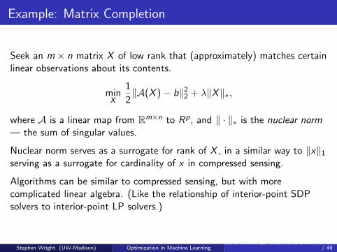
Example: Matrix Completion

Seek an m × n matrix X of low rank that (approximately) matches certainlinear observations about its contents.

minX

1

2‖A(X )− b‖22 + λ‖X‖∗,

where A is a linear map from Rm×n to Rp, and ‖ · ‖∗ is the nuclear norm— the sum of singular values.

Nuclear norm serves as a surrogate for rank of X , in a similar way to ‖x‖1serving as a surrogate for cardinality of x in compressed sensing.

Algorithms can be similar to compressed sensing, but with morecomplicated linear algebra. (Like the relationship of interior-point SDPsolvers to interior-point LP solvers.)


/ 49

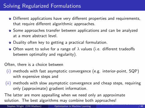
Solving Regularized Formulations

Different applications have very different properties and requirements,that require different algorithmic approaches.

Some approaches transfer between applications and can be analyzedat a more abstract level.

Duality often key to getting a practical formulation.

Often want to solve for a range of λ values (i.e. different tradeoffsbetween optimality and regularity).

Often, there is a choice between

(i) methods with fast asymptotic convergence (e.g. interior-point, SQP)with expensive steps and

(ii) methods with slow asymptotic convergence and cheap steps, requiringonly (approximate) gradient information.

The latter are more appealling when we need only an approximatesolution. The best algorithms may combine both approaches!


/ 49

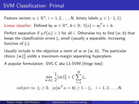
SVM Classification: Primal

Feature vectors xi ∈ Rn, i = 1, 2, . . . ,N, binary labels yi ∈ −1, 1.

Linear classifier: Defined by w ∈ Rn, b ∈ R: f (x) = wTi x + b.

Perfect separation if yi f (xi ) ≥ 1 for all i . Otherwise try to find (w , b) thatkeeps the classification errors ξi small (usually a separable, increasingfunction of ξi ).

Usually include in the objective a norm of w or (w , b). The particularchoice ‖w‖22 yields a maximum-margin separating hyperplane.

A popular formulation: SVC-C aka L1-SVM (hinge loss):

minw ,b,ξ

1

2‖w‖22 + C

N∑i=1

ξi ,

subject to ξi ≥ 0, yi (wT xi + b) ≥ 1− ξi , i = 1, 2, . . . ,N.


/ 49

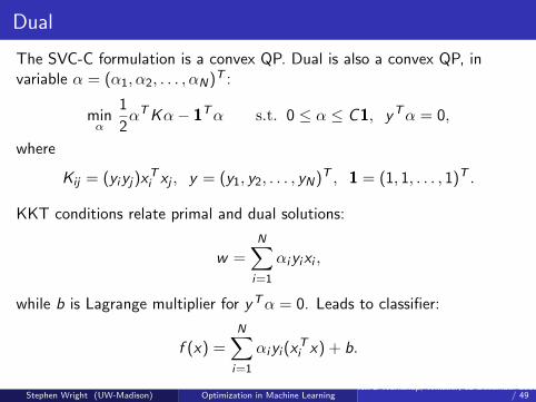
Dual

The SVC-C formulation is a convex QP. Dual is also a convex QP, invariable α = (α1, α2, . . . , αN)T :

minα

1

2αTKα− 1Tα s.t. 0 ≤ α ≤ C1, yTα = 0,

where

Kij = (yiyj)xTi xj , y = (y1, y2, . . . , yN)T , 1 = (1, 1, . . . , 1)T .

KKT conditions relate primal and dual solutions:

w =N∑

i=1

αiyixi ,

while b is Lagrange multiplier for yTα = 0. Leads to classifier:

f (x) =N∑

i=1

αiyi (xTi x) + b.


/ 49

Kernel Trick, RKHS

For a more powerful classifier, can project feature vector xi into ahigher-dimensional space via a function φ : Rn → Rt and classify in thatspace. Dual formulation is the same, except for redefined K :

Kij = (yiyj)φ(xi )Tφ(xj).

Leads to classifier:

f (x) =N∑

i=1

αiyiφ(xi )Tφ(x) + b.

Don’t actually need to use φ at all, just inner products φ(x)Tφ(x). Insteadof φ, work with a kernel function k : Rn × Rn → R.

If k is continuous, symmetric in arguments, and positive definite (Mercerkernel), there exists a Hilbert space and a function φ in this space suchthat k(x , x) = φ(x)Tφ(x).


/ 49

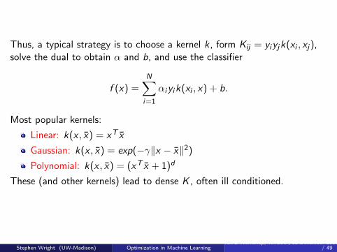
Thus, a typical strategy is to choose a kernel k, form Kij = yiyjk(xi , xj),solve the dual to obtain α and b, and use the classifier

f (x) =N∑

i=1

αiyik(xi , x) + b.

Most popular kernels:

Linear: k(x , x) = xT x

Gaussian: k(x , x) = exp(−γ‖x − x‖2)Polynomial: k(x , x) = (xT x + 1)d

These (and other kernels) lead to dense K , often ill conditioned.


/ 49

Solving the Primal and (Kernelized) Dual

Many methods have been proposed for solving either the primalformulation of linear classification, or the dual (usually with kernel form).Research continues apace.

Most are based on optimization methods, or can be interpreted using theoptimization framework.

Methods compared via a variety of metrics:

CPU time to find solution of given quality (error rate, or targetobjective value).

Theoretical efficiency.

Data storage requirements.

(Simplicity.) (Parallelizability.)

We’ll review several approaches, emphasizing recent developments andlarge-scale problems.


/ 49

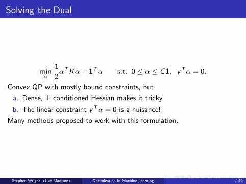
Solving the Dual

minα

1

2αTKα− 1Tα s.t. 0 ≤ α ≤ C1, yTα = 0.

Convex QP with mostly bound constraints, but

a. Dense, ill conditioned Hessian makes it tricky

b. The linear constraint yTα = 0 is a nuisance!

Many methods proposed to work with this formulation.


/ 49

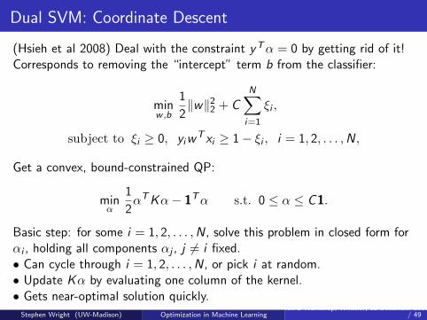
Dual SVM: Coordinate Descent

(Hsieh et al 2008) Deal with the constraint yTα = 0 by getting rid of it!Corresponds to removing the “intercept” term b from the classifier:

minw ,b

1

2‖w‖22 + C

N∑i=1

ξi ,

subject to ξi ≥ 0, yiwT xi ≥ 1− ξi , i = 1, 2, . . . ,N,

Get a convex, bound-constrained QP:

minα

1

2αTKα− 1Tα s.t. 0 ≤ α ≤ C1.

Basic step: for some i = 1, 2, . . . ,N, solve this problem in closed form forαi , holding all components αj , j 6= i fixed.• Can cycle through i = 1, 2, . . . ,N, or pick i at random.• Update Kα by evaluating one column of the kernel.• Gets near-optimal solution quickly.


/ 49

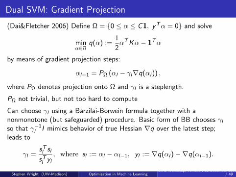
Dual SVM: Gradient Projection

(Dai&Fletcher 2006) Define Ω = 0 ≤ α ≤ C1, yTα = 0 and solve

minα∈Ω

q(α) :=1

2αTKα− 1Tα

by means of gradient projection steps:

αl+1 = PΩ (αl − γl∇q(αl)) ,

where PΩ denotes projection onto Ω and γl is a steplength.

PΩ not trivial, but not too hard to compute

Can choose γl using a Barzilai-Borwein formula together with anonmonotone (but safeguarded) procedure. Basic form of BB chooses γl

so that γ−1l I mimics behavior of true Hessian ∇q over the latest step;

leads to

γl =sTl sl

sTl yl

, where sl := αl − αl−1, yl := ∇q(αl)−∇q(αl−1).


/ 49

Dual SVM: Decomposition

Many algorithms for dual formulation make use of decomposition: Choosea subset of components of α and (approximately) solve a subproblem injust these components, fixing the other components at one of theirbounds. Usually maintain feasible α throughout.

Many variants, distinguished by strategy for selecting subsets, size ofsubsets, inner-loop strategy for solving the reduced problem.

SMO: (Platt 1998). Subproblem has two components.

SMVlight: (Joachims 1998). Use chooses subproblem size (usually small);components selected with a first-order heuristic. (Could use an `1 penaltyas surrogate for cardinality constraint?)

PGPDT: (Zanni, Serafini, Zanghirati 2006) Decomposition, with gradientprojection on the subproblems. Parallel implementation.


/ 49

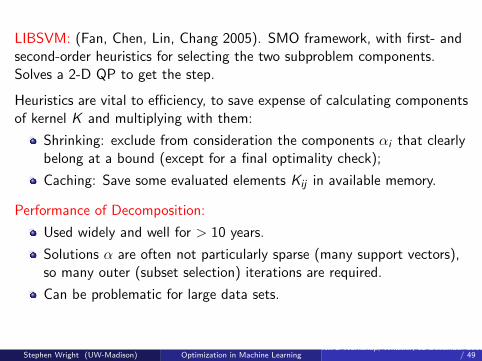
LIBSVM: (Fan, Chen, Lin, Chang 2005). SMO framework, with first- andsecond-order heuristics for selecting the two subproblem components.Solves a 2-D QP to get the step.

Heuristics are vital to efficiency, to save expense of calculating componentsof kernel K and multiplying with them:

Shrinking: exclude from consideration the components αi that clearlybelong at a bound (except for a final optimality check);

Caching: Save some evaluated elements Kij in available memory.

Performance of Decomposition:

Used widely and well for > 10 years.

Solutions α are often not particularly sparse (many support vectors),so many outer (subset selection) iterations are required.

Can be problematic for large data sets.


/ 49

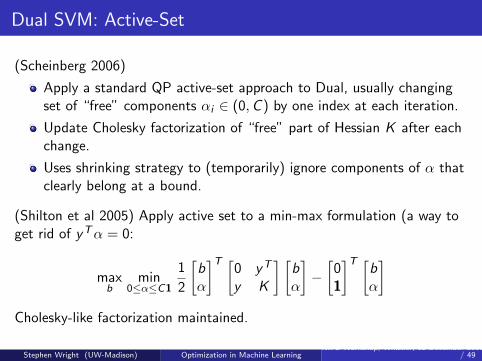
Dual SVM: Active-Set

(Scheinberg 2006)

Apply a standard QP active-set approach to Dual, usually changingset of “free” components αi ∈ (0,C ) by one index at each iteration.

Update Cholesky factorization of “free” part of Hessian K after eachchange.

Uses shrinking strategy to (temporarily) ignore components of α thatclearly belong at a bound.

(Shilton et al 2005) Apply active set to a min-max formulation (a way toget rid of yTα = 0:

maxb

min0≤α≤C1

1

2

[bα

]T [0 yT

y K

] [bα

]−

[01

]T [bα

]Cholesky-like factorization maintained.


/ 49

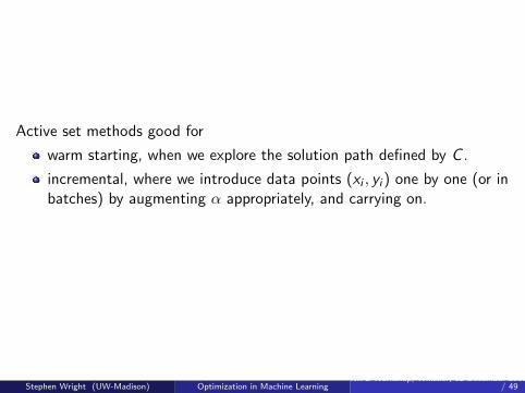
Active set methods good for

warm starting, when we explore the solution path defined by C .

incremental, where we introduce data points (xi , yi ) one by one (or inbatches) by augmenting α appropriately, and carrying on.


/ 49

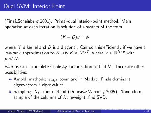
Dual SVM: Interior-Point

(Fine&Scheinberg 2001). Primal-dual interior-point method. Mainoperation at each iteration is solution of a system of the form

(K + D)u = w ,

where K is kernel and D is a diagonal. Can do this efficiently if we have alow-rank approximation to K , say K ≈ VV T , where V ∈ RN×p withp N.

F&S use an incomplete Cholesky factorization to find V . There are otherpossibilities:

Arnoldi methods: eigs command in Matlab. Finds dominanteigenvectors / eigenvalues.

Sampling: Nystrom method (Drineas&Mahoney 2005). Nonuniformsample of the columns of K , reweight, find SVD.


/ 49

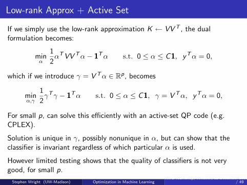
Low-rank Approx + Active Set

If we simply use the low-rank approximation K ← VV T , the dualformulation becomes:

minα

1

2αTVV Tα− 1Tα s.t. 0 ≤ α ≤ C1, yTα = 0,

which if we introduce γ = V Tα ∈ Rp, becomes

minα,γ

1

2γTγ − 1Tα s.t. 0 ≤ α ≤ C1, γ = V Tα, yTα = 0,

For small p, can solve this efficiently with an active-set QP code (e.g.CPLEX).

Solution is unique in γ, possibly nonunique in α, but can show that theclassifier is invariant regardless of which particular α is used.

However limited testing shows that the quality of classifiers is not verygood, for small p.


/ 49

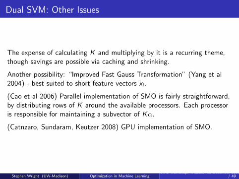
Dual SVM: Other Issues

The expense of calculating K and multiplying by it is a recurring theme,though savings are possible via caching and shrinking.

Another possibility: “Improved Fast Gauss Transformation” (Yang et al2004) - best suited to short feature vectors xi .

(Cao et al 2006) Parallel implementation of SMO is fairly straightforward,by distributing rows of K around the available processors. Each processoris responsible for maintaining a subvector of Kα.

(Catnzaro, Sundaram, Keutzer 2008) GPU implementation of SMO.


/ 49

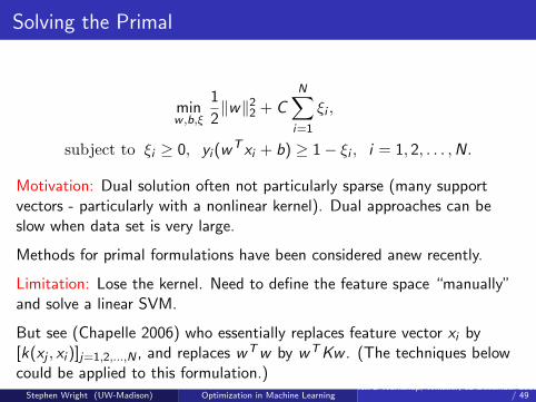
Solving the Primal

minw ,b,ξ

1

2‖w‖22 + C

N∑i=1

ξi ,


Motivation: Dual solution often not particularly sparse (many supportvectors - particularly with a nonlinear kernel). Dual approaches can beslow when data set is very large.

Methods for primal formulations have been considered anew recently.

Limitation: Lose the kernel. Need to define the feature space “manually”and solve a linear SVM.

But see (Chapelle 2006) who essentially replaces feature vector xi by[k(xj , xi )]j=1,2,...,N , and replaces wTw by wTKw . (The techniques belowcould be applied to this formulation.)


/ 49

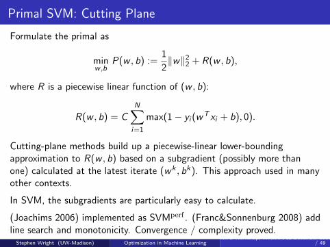
Primal SVM: Cutting Plane

Formulate the primal as

minw ,b

P(w , b) :=1

2‖w‖22 + R(w , b),

where R is a piecewise linear function of (w , b):

R(w , b) = CN∑

i=1

max(1− yi (wT xi + b), 0).

Cutting-plane methods build up a piecewise-linear lower-boundingapproximation to R(w , b) based on a subgradient (possibly more thanone) calculated at the latest iterate (wk , bk). This approach used in manyother contexts.

In SVM, the subgradients are particularly easy to calculate.

(Joachims 2006) implemented as SVMperf . (Franc&Sonnenburg 2008) addline search and monotonicity. Convergence / complexity proved.


/ 49

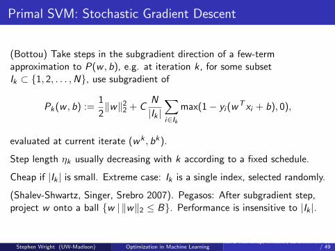
Primal SVM: Stochastic Gradient Descent

(Bottou) Take steps in the subgradient direction of a few-termapproximation to P(w , b), e.g. at iteration k, for some subsetIk ⊂ 1, 2, . . . ,N, use subgradient of

Pk(w , b) :=1

2‖w‖22 + C

N

|Ik |∑i∈Ik

max(1− yi (wT xi + b), 0),

evaluated at current iterate (wk , bk).

Step length ηk usually decreasing with k according to a fixed schedule.

Cheap if |Ik | is small. Extreme case: Ik is a single index, selected randomly.

(Shalev-Shwartz, Singer, Srebro 2007). Pegasos: After subgradient step,project w onto a ball w | ‖w‖2 ≤ B. Performance is insensitive to |Ik |.


/ 49

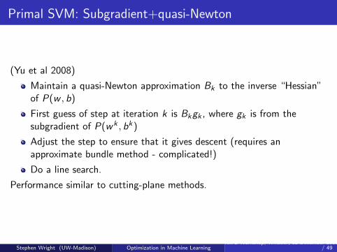
Primal SVM: Subgradient+quasi-Newton

(Yu et al 2008)

Maintain a quasi-Newton approximation Bk to the inverse “Hessian”of P(w , b)

First guess of step at iteration k is Bkgk , where gk is from thesubgradient of P(wk , bk)

Adjust the step to ensure that it gives descent (requires anapproximate bundle method - complicated!)

Do a line search.

Performance similar to cutting-plane methods.


/ 49

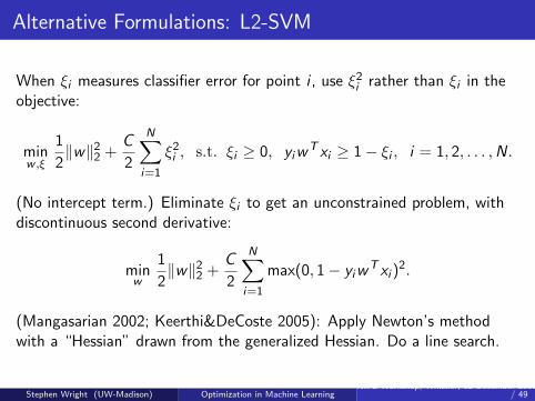
Alternative Formulations: L2-SVM

When ξi measures classifier error for point i , use ξ2i rather than ξi in the

objective:

minw ,ξ

1

2‖w‖22 +

C

2

N∑i=1

ξ2i , s.t. ξi ≥ 0, yiw

T xi ≥ 1− ξi , i = 1, 2, . . . ,N.

(No intercept term.) Eliminate ξi to get an unconstrained problem, withdiscontinuous second derivative:

minw

1

2‖w‖22 +

C

2

N∑i=1

max(0, 1− yiwT xi )

2.

(Mangasarian 2002; Keerthi&DeCoste 2005): Apply Newton’s methodwith a “Hessian” drawn from the generalized Hessian. Do a line search.


/ 49

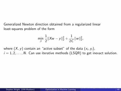
Generalized Newton direction obtained from a regularized linearleast-squares problem of the form

minβ

1

2‖Xw − y‖22 +

1

2C‖w‖22,

where (X , y) contain an “active subset” of the data (xi , yi ),i = 1, 2, . . . ,N. Can use iterative methods (LSQR) to get inexact solution.


/ 49

Alternative Formulations: ‖w‖1.

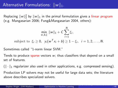
Replacing ‖w‖22 by ‖w‖1 in the primal formulation gives a linear program(e.g. Mangasarian 2006; Fung&Mangasarian 2004, others):

minw ,b,ξ

‖w‖1 + CN∑

i=1

ξi ,


Sometimes called “1-norm linear SVM.”

Tends to produce sparse vectors w ; thus classifiers that depend on a smallset of features.

(‖ · ‖1 regularizer also used in other applications, e.g. compressed sensing).

Production LP solvers may not be useful for large data sets; the literatureabove describes specialized solvers.


/ 49

Elastic Net

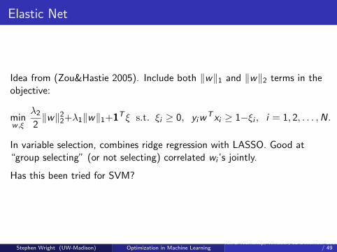
Idea from (Zou&Hastie 2005). Include both ‖w‖1 and ‖w‖2 terms in theobjective:

minw ,ξ

λ2

2‖w‖22+λ1‖w‖1+1T ξ s.t. ξi ≥ 0, yiw

T xi ≥ 1−ξi , i = 1, 2, . . . ,N.

In variable selection, combines ridge regression with LASSO. Good at“group selecting” (or not selecting) correlated wi ’s jointly.

Has this been tried for SVM?


/ 49

Logistic Regression

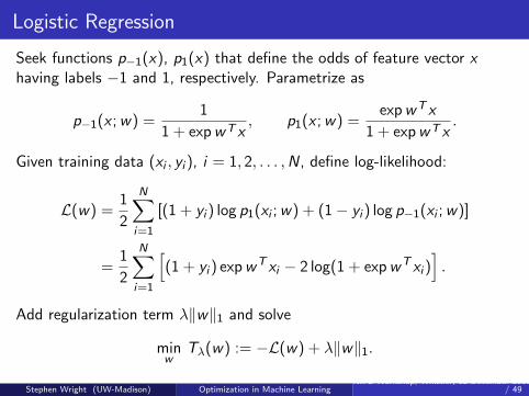
Seek functions p−1(x), p1(x) that define the odds of feature vector xhaving labels −1 and 1, respectively. Parametrize as

p−1(x ;w) =1

1 + expwT x, p1(x ;w) =

expwT x

1 + expwT x.

Given training data (xi , yi ), i = 1, 2, . . . ,N, define log-likelihood:

L(w) =1

2

N∑i=1

[(1 + yi ) log p1(xi ;w) + (1− yi ) log p−1(xi ;w)]

=1

2

N∑i=1

[(1 + yi ) expwT xi − 2 log(1 + expwT xi )

].

Add regularization term λ‖w‖1 and solve

minw

Tλ(w) := −L(w) + λ‖w‖1.


/ 49

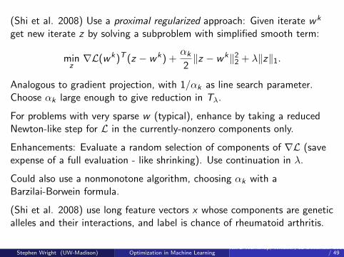
(Shi et al. 2008) Use a proximal regularized approach: Given iterate wk

get new iterate z by solving a subproblem with simplified smooth term:

minz∇L(wk)T (z − wk) +

αk

2‖z − wk‖22 + λ‖z‖1.

Analogous to gradient projection, with 1/αk as line search parameter.Choose αk large enough to give reduction in Tλ.

For problems with very sparse w (typical), enhance by taking a reducedNewton-like step for L in the currently-nonzero components only.

Enhancements: Evaluate a random selection of components of ∇L (saveexpense of a full evaluation - like shrinking). Use continuation in λ.

Could also use a nonmonotone algorithm, choosing αk with aBarzilai-Borwein formula.

(Shi et al. 2008) use long feature vectors x whose components are geneticalleles and their interactions, and label is chance of rheumatoid arthritis.


/ 49

New Tool: Optimal Gradient Methods

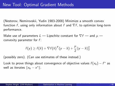
(Nesterov, Nemirovskii, Yudin 1983-2008) Minimize a smooth convexfunction f , using only information about f and ∇f , to optimize long-termperformance.

Make use of parameters L — Lipschitz constant for ∇f — and µ —convexity parameter for f :

f (y) ≥ f (x) +∇f (x)T (y − x) +µ

2‖y − x‖22

(possibly zero). (Can use estimates of these instead.)

Look to prove things about convergence of objective values f (xk)− f ∗ aswell as iterates ‖xk − x∗‖.


/ 49

Basic Gradient Methods

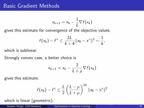
xk+1 = xk −1

L∇f (xk)

gives this estimate for convergence of the objective values:

f (xk)− f ∗ ≤ 2L

k + 4‖x0 − x∗‖2 ∼ 1

k,

which is sublinear.

Strongly convex case, a better choice is

xk+1 = xk −2

L + µ∇f (xk)

gives this estimate:

f (xk)− f ∗ ≤ L

2

(L− µ

L + µ

)2k

‖x0 − x∗‖2

which is linear (geometric).Stephen Wright (UW-Madison) Optimization in Machine Learning

NIPS Workshop, Whistler, 12 December 2008 37/ 49

Optimal Rates

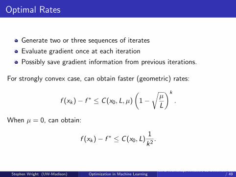
Generate two or three sequences of iterates

Evaluate gradient once at each iteration

Possibly save gradient information from previous iterations.

For strongly convex case, can obtain faster (geometric) rates:

f (xk)− f ∗ ≤ C (x0, L, µ)

(1−

√µ

L

)k

.

When µ = 0, can obtain:

f (xk)− f ∗ ≤ C (x0, L)1

k2.


/ 49

Typical Schemes

Strongly convex (µ > 0): Start with y0 = x0 and generate:

xk+1 = yk −1

L∇f (yk); (1)

yk+1 = xk+1 +

√L−√µ√

L +√

µ(xk+1 − xk). (2)

Weakly convex: more complicated linear combination. x step is still (1),but y step is

yk+1 = xk+1 + βk(xk+1 − xk),

where

βk = αk(1− αk)/(α2k + αk+1),

α2k+1 = (1− αk+1)α

2k + qαk+1

with q = µ/L, y0 = x0, and some α0 ∈ (0, 1).Stephen Wright (UW-Madison) Optimization in Machine Learning


Extensions

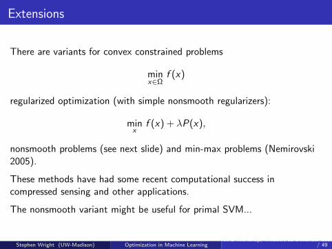
There are variants for convex constrained problems

minx∈Ω

f (x)

regularized optimization (with simple nonsmooth regularizers):

minx

f (x) + λP(x),

nonsmooth problems (see next slide) and min-max problems (Nemirovski2005).

These methods have had some recent computational success incompressed sensing and other applications.

The nonsmooth variant might be useful for primal SVM...


/ 49

Nesterov: Smoothing Nonsmooth Problems

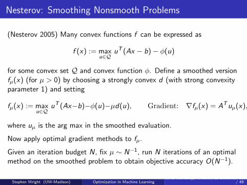
(Nesterov 2005) Many convex functions f can be expressed as

f (x) := maxu∈Q

uT (Ax − b)− φ(u)

for some convex set Q and convex function φ. Define a smoothed versionfµ(x) (for µ > 0) by choosing a strongly convex d (with strong convexityparameter 1) and setting

fµ(x) := maxu∈Q

uT (Ax−b)−φ(u)−µd(u), Gradient: ∇fµ(x) = ATuµ(x),

where uµ is the arg max in the smoothed evaluation.

Now apply optimal gradient methods to fµ.

Given an iteration budget N, fix µ ∼ N−1, run N iterations of an optimalmethod on the smoothed problem to obtain objective accuracy O(N−1).


/ 49

New Tool: Primal-Dual Gradient Projection

Consider a saddle point (min-max) problem

minv∈V

maxx∈X

`(v , x),

with `(·, x) convex for all x ∈ X and `(v , ·) concave for all v ∈ V , and Vand X are convex sets.

(When ` is quadratic and V , X are polyhedral, this is Rockafellar’s ELQP.)

Many convex optimization problems can be formulated naturally in thisframework.

Primal-dual gradient projection procedure is

xk+1 ← PX (xk + τk∇x`(vk , xk)),

vk+1 ← PV (vk − σk∇v `(vk , xk+1)),

where τk and σk are positive steplengths.


/ 49

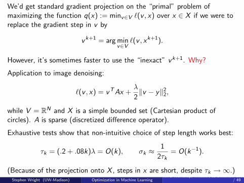
We’d get standard gradient projection on the “primal” problem ofmaximizing the function q(x) := minv∈V `(v , x) over x ∈ X if we were toreplace the gradient step in v by

vk+1 = arg minv∈V

`(v , xk+1).

However, it’s sometimes faster to use the “inexact” vk+1. Why?

Application to image denoising:

`(v , x) = vTAx +λ

2‖v − y‖22,

while V = RN and X is a simple bounded set (Cartesian product ofcircles). A is sparse (discretized difference operator).

Exhaustive tests show that non-intuitive choice of step length works best:

τk = (.2 + .08k)λ = O(k), σk ≈1

2τk= O(k−1).

(Because of the projection onto X , steps in x are short, despite τk →∞.)Stephen Wright (UW-Madison) Optimization in Machine Learning


There are many ways to view this approach, but none has yet yieldedan understanding of its excellent practical performance.

Does its usefulness extend beyond image reconstruction, e.g. to SVMformulations?


/ 49

References

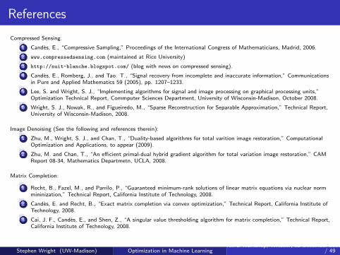
Compressed Sensing.

1 Candes, E., “Compressive Sampling,” Proceedings of the International Congress of Mathematicians, Madrid, 2006.

2 www.compressedsensing.com (maintained at Rice University)

3 http://nuit-blanche.blogspot.com/ (blog with news on compressed sensing).

4 Candes, E., Romberg, J., and Tao. T., “Signal recovery from incomplete and inaccurate information,” Communicationsin Pure and Applied Mathematics 59 (2005), pp. 1207–1233.

5 Lee, S. and Wright, S. J., “Implementing algorithms for signal and image processing on graphical processing units,”Optimization Technical Report, Commputer Sciences Department, University of Wisconsin-Madison, October 2008.

6 Wright, S. J., Nowak, R., and Figueiredo, M., “Sparse Reconstruction for Separable Approximation,” Technical Report,University of Wisconsin-Madison, 2008.

Image Denoising (See the following and references therein):

1 Zhu, M., Wright, S. J., and Chan, T., “Duality-based algorithms for total varition image restoration,” ComputationalOptimization and Applications, to appear (2009).

2 Zhu, M. and Chan, T., “An efficient primal-dual hybrid gradient algorithm for total variation image restoration,” CAMReport 08-34, Mathematics Departmetn, UCLA, 2008.

Matrix Completion:

1 Recht, B., Fazel, M., and Parrilo, P., “Guaranteed minimum-rank solutions of linear matrix equations via nuclear normmininization,” Technical Report, California Institute of Technology, 2008.

2 Candes, E. and Recht, B., “Exact matrix completion via convex optimization,” Technical Report, California Institute ofTechnology, 2008.

3 Cai, J. F., Candes, E., and Shen, Z., “A singular value thresholding algorithm for matrix completion,” Technical Report,California Institute of Technology, 2008.


/ 49

Dual SVM (papers cited in talk):

1 Hsieh, C.-J., Chang, K.-W., Lin, C.-J., Keerthi, S. S., and Sundararajan, S., “A Dual coordinate descent method forlarge-scale linear SVM”, Proceedings of teh 25th ICML, Helsinki, 2008.

2 Dai, Y.-H. and Fletcher, R., “New algorithms for singly linearly consrtained quadratic programming subject to lower andupper bounds,” Mathematical Programming, Series A, 106 (2006), pp. 403–421.

3 Platt, J., “Fast training of support vector machines using sequential minimal optimization,” Chapter 12 in Advances inKernel Methods (B. Scholkopf, C. Burges, and A. Smola, eds), MIT Press, Cambridge, 1998.

4 Joachims, T., “Making large-scale SVM learning practical,” Chapter 11 in Advances in Kernel Methods (B. Scholkopf,C. Burges, and A. Smola, eds), MIT Press, Cambridge, 1998.

5 Zanni, L., Serafini, T., and Zanghirati, G., “Parallel software for training large-scale support vector machines onmultiprocessor systems,” JMLR 7 (206), pp. 1467–1492.

6 Fan, R.-E., Chen, P.-H., and Lin, C.-J., “Working set selection using second-order information for training SVM,” JMLR6 (2005), pp. 1889–1918.

7 Chen, P.-H., Fan, R.-E., and Lin, C.-J., “A study on SMO-type decomposition methods for support vector machines,”IEEE Transactions on Neural Networks 17 (2006), pp. 892–908.

8 Scheinberg, K. “An efficient implementation of an active-set method for SVMs,” JMLR 7 (2006), pp. 2237-2257.

9 Shilton, A., Palaniswami, M., Ralph, D., and Tsoi, A. C., “Incremental training of support vector machines,” IEEETransactions on Neural Networks 16 (2005), pp. 114–131.

10 Fine, S., and Scheinberg, K., “Efficient SVM training using low-rank kernel representations,” JMLR 2 (2001), pp.243–264.

11 Drineas, P. and Mahoney, M., “On the Nystrom method for approximating a Gram matrix for improved kernel-basedlearning,” JMLR 6 (2005), pp. 2153–2175.

12 Yang, C., Duraiswami, R., and Davis, L., “Efficient kernel machines using the improved fast Gauss transform,” 2004.

13 Cao, L. J., Keerthi, S. S., Ong, C.-J., Zhang, J. Q., Periyathamby, U., Fu, X. J., and Lee, H. P., “Parallel sequentialminimal optmization for the training of support vector machines,”IEEE Transactions on Neural Networks 17 (2006), pp.1039–1049.

14 Catanzaro, B., Sundaram, N., and Keutzer, K., “Fast support vector machine training and classification on graphicsprocessors,” Proceedings of the 25th ICML, Helsinki, Finland, 2008.


/ 49

Primal SVM papers (cited in talk):

1 Chappelle, O., “Training a support vector machine in the primal,” Neural Computation, in press (2008).

2 Shalev-Schwartz, S., Singer, Y., and Srebro, N., “Pegasos: Primal estimated sub-gradient solver for SVM,” Proceedingsof the 24th ICML, Corvallis, Oregon, 2007.

3 Joachims, T., “Training linear SVMs in linear time,” KDD ’06, 2006.

4 Franc, V., and Sonnenburg, S., “Optimized cutting plane algorithm for support vector machines,” in Proceedings of the25th ICML, Helsinki, 2008.

5 Bottou, L. and Bousquet, O., “The tradeoffs of large-scale learning,” in Advances in Neural Information ProcessingSystems 20 (2008), pp. 161–168.

6 Yu, J., Vishwanathan, S. V. N., Gunter, S., and Schraudolph, N. N., “A quasi-Newton approach to nonsmooth convexoptimization,” in Proceedings of the 25th ICML, Helsinki, 2008.

7 Keerthi, S. S. and DeCoste, D., “A Modified finite Newton method for fast solution of large-scale linear SVMs,” JMLR6 (2005), pp. 341–361.

8 Mangasarian, O. L., “A finite Newton method for classification,” Optimization Methods and Software 17 (2002), pp.913–929.

9 Mangasarian, O. L., “Exact 1-norm support vector machines via unconstrained convex differentiable minimization,”JMLR 7 (2006), 1517–1530.

10 Fung, G. and Mangasarian, O. L., “A Feature selection Newton method for support vector machine classification,”Computational Optimization and Applications 28 (2004), pp. 185–202.

11 Zou, H. and Hastie, T., “Regularization and variable selection via the elastic net,” J. R¿ Statist. Soc. B 67 (2005), pp.301–320.

Logistic Regression:

1 Shi, W., Wahba, G., Wright, S. J., lee, K., Klein, R., and Klein, B., “LASSO-Patternsearch algorithm with applicationto ophthalmology data,” Statistics and its Interface 1 (2008), pp. 137–153.


/ 49

Optimal Gradient Methods:

1 Nesterov, Y., “A method for unconstrained convex problem with the rate of convergence O(1/k2),” Doklady AN SSR269 (1983), pp. 543–547.

2 Nesterov, Y., Introductory Lectures on Convex Optimization: A Basic Course, Kluwer, 2004.

3 Nesterov. Y., “Smooth minimization of nonsmooth functions,” Mathematical Programming A 103 (2005), pp. 127–152.

4 Nemirovski, A., “Prox-method with rate of convergence O(1/t) for variational inequalities with Lipschitz continuousmonotone operators and smooth convex-concave saddle point problems,” SIAM J. Optimization 15 (2005), pp. 229–251.


/ 49

THE END


/ 49

Documents

Optimization in Machine Learning - University of Wisconsinâ€“Madison