OPTIMAL WIND BRACING SYSTEMS FOR MULTI-STOREY STEEL BUILDINGS

A THESIS SUBMITTED TOTHE GRADUATE SCHOOL OF NATURAL AND APPLIED SCIENCES

OFMIDDLE EAST TECHNICAL UNIVERSITY

BY

İLYAS YILDIRIM

IN PARTIAL FULFILLMENT OF THE REQUIREMENTSFOR

THE DEGREE OF MASTER OF SCIENCEIN

CIVIL ENGINEERING

AUGUST 2009

Approval of the thesis:

OPTIMAL WIND BRACING SYSTEMS FOR MULTI-STOREY STEEL BUILDINGS

submitted by İLYAS YILDIRIM in partial fulfillment of the requirements for the degree of Master of Science in Civil Engineering Department, Middle East Technical University by,

Prof. Dr. Canan ÖzgenDean, Graduate School of Natural and Applied Sciences

Prof. Dr. Güney ÖzcebeHead of Department, Civil Engineering

Assoc. Prof. Dr. Oğuzhan HasançebiSupervisor, Civil Engineering Dept., METU

Examining Committee Members:

Prof. Dr. Turgut TokdemirEngineering Sciences Dept., METU

Assoc. Prof. Dr. Oğuzhan HasançebiCivil Engineering Dept., METU

Assoc. Prof. Dr. Ahmet TürerCivil Engineering Dept., METU

Assoc. Prof. Dr. Cem TopkayaCivil Engineering Dept., METU

Assist. Prof. Dr. Alp CanerCivil Engineering Dept., METU

Date: August 07, 2009

I hereby declare that all information in this document has been obtained and presented in accordance with academic rules and ethical conduct. I also declare that, as required by these rules and conduct, I have fully cited and referenced all material and results that are not original to this work.

Name, Last Name : İlyas Yıldırım

Signature :

iv

ABSTRACT

OPTIMAL WIND BRACING SYSTEMS FOR MULTI-STOREY STEEL BUILDINGS

Yıldırım, İlyas

M.Sc., Department of Civil Engineering

Supervisor: Assoc. Prof. Oğuzhan Hasançebi

August 2009, 130 pages

The major concern in the design of the multi-storey buildings is the structure to

have enough lateral stability to resist wind forces. There are different ways to

limit the lateral drift. First method is to use unbraced frame with moment-

resisting connections. Second one is to use braced frames with moment-

resisting connections. Third one is to use pin-jointed connections instead of

moment-resisting one and using bracings. Finally braced frame with both

moment-resisting and pin-jointed connections is a solution.

There are lots of bracing models and the designer should choose the

appropriate one. This thesis investigates optimal lateral bracing systems in

v

steel structures. The method selects appropriate sections for beams, columns

and bracings, from a given steel section set, and obtains a design with least

weight. After obtaining the best designs in case of weight, cost analysis of all

structures are carried out so that the most economical model is found. For this

purpose evolution strategies optimization method is used which is a member of

the evolutionary algorithms search techniques.

First optimum design of steel frames is introduced in the thesis. Then evolution

strategies technique is explained. This is followed by some information about

design loads and bracing systems are given. It is continued by the cost analysis

of the models. Finally numerical examples are presented. Optimum designs of

three different structures, comprising twelve different bracing models, are

carried out. The calculations are carried out by a computer program

(OPTSTEEL) which is recently developed to achieve size optimization design of

skeletal structures.

Keywords: Optimization, Structural Optimization, Evolutionary Algorithms,

Evolution Strategies, Steel Frames, Optimal Bracing Systems.

vi

ÖZ

ÇOK KATLI ÇELİK BİNALARIN OPTİMUM RÜZGAR BAĞLANTI TASARIMLARI

Yıldırım, İlyas

Yüksek Lisans, İnşaat Mühendisliği Bölümü

Tez Yöneticisi: Doç Dr. Oğuzhan Hasançebi

Ağustos 2009, 130 sayfa

Çok katlı çelik yapıların tasarımındaki en önemli nokta yapının, rüzgar

yüklerine dayanabilmesi için, yeterli yatay kararlılığa sahip olmasıdır.

Binalardaki yatay ötelenmeyi belirli sınırlar içinde tutmak için farklı yollar

mevcuttur. Birinci yol, bütün kolon kiriş bağlantılarını rijit yapmaktır. İkinci

yöntem bu yapılara bir de yatay çapraz elemanları monte etmektir. Üçüncü yol

kolon kiriş bağlantılarını mafsallı yapmak ve yatay çapraz elemanları

kullanmaktır. Son yol ise hem rijit hem de mafsallı bağlantıları kullanmak ve

yatay çapraz elemanları kullanmaktır.

vii

Birçok çapraz modeli mevcuttur ve tasarımcının bunların arasından en uygun

olanını seçmelidir. Bu tez, çelik yapıların optimum çapraz tasarımlarını

anlatmaktadır. Metod, kirişler, kolonlar ve çapraz elemanları için en uygun

kesiti, daha önceden tanımlanmış kesitler listesinden, seçer ve en hafif dizaynı

bulur. Daha sonra bütün modeller için maliyet analizleri yapılmaktadır ve

böylece en ekonomik model bulunabilmektedir. Bu amaç için, evrimsel

algoritmalar üyesi olan, evrimsel stratejiler kullanılır.

İlk başta çelik yapıların optimum tasarımları anlatılmaktadır. Daha sonra

evrimsel algoritmalara değinilmiştir. Onu takiben, rüzgar yükleri ve çapraz

modelleriyle ilgili bazı bilgiler verilmiştir. Daha sonra yapıların maliyet

analizleri anlatılmaktadır. Son olarak da bazı örnek problemler sunulmuştur.

Üç farklı yapının, oniki farklı çapraz modeli kullanılarak analizleri yapılmıştır.

Bu prosedür, son yıllarda geliştirilen ve yapıların kesit opitmizasyonunu

sağlayan, OPTSTEEL ile sürdürülmüştür.

Anahtar Kelimeler: Optimizasyon, Yapı Optimizasyonu, Evrimsel Algoritmalar,

Evrimsel Stratejiler, Çelik Yapılar, Optimum Çapraz Tasarımı.

To Kaan

ix

ACKNOWLEDGMENTS

I would like to express my deepest gratitude to my thesis supervisor Assoc.

Prof. Dr. Oğuzhan Hasançebi for his endless guidance and patience throughout

my study. Studying with such energetic and idealist instructor is a real pleasure

for me. Without his comments, it would have been impossible to complete this

thesis.

I am proud of being a member of Middle East Technical University and feel

myself lucky for having a chance to be taught by such talented and intellectual

instructors. I want to thank to all members of my University.

Finally, I am grateful to my mother, sister and father. They always supported

me for whatever I deal with, without waiting for a counterpart.

x

TABLE OF CONTENTS

ABSTRACT................................................................................................................................iv

ÖZ.................................................................................................................................................vi

ACKNOWLEDGMENTS......................................................................................................... ix

TABLE OF CONTENTS........................................................................................................... x

LIST OF TABLES .................................................................................................................. xiii

LIST OF FIGURES ................................................................................................................ xiv

CHAPTERS

1. INTRODUCTION..................................................................................................................1

1.1 Previous Studies ...................................................................................................3

1.2 Optimization of Steel Frames ..........................................................................5

1.3 Evolutionary Algorithms ...................................................................................6

1.4 Evolution Strategies ............................................................................................7

1.5 Aim and Scope of the Study ..............................................................................8

2. OPTIMUM DESIGN OF STEEL FRAMES USING EVOLUTION STRATEGIES10

2.1 Optimization........................................................................................................ 10

2.2 Design Optimization of Steel Frames......................................................... 13

2.3 Evolutionary Algorithms ................................................................................ 18

2.4 Evolution Strategies ......................................................................................... 20

xi

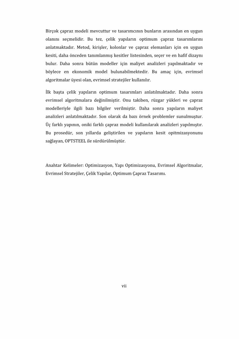
2.4.1 Optimization Routine .................................................................................. 20

2.4.2 ESs for Continuous Variables ................................................................... 23

2.4.2.1 Representation of an Individual and Initial Population........... 23

2.4.2.2 Constraint Handling and Evaluation of Population ................... 24

2.4.2.3 Recombination ......................................................................................... 26

2.4.2.4 Mutation...................................................................................................... 28

2.4.2.5 Selection...................................................................................................... 35

2.4.2.6 Termination............................................................................................... 36

2.4.3 ESs for Discrete Variables.......................................................................... 36

2.4.3.1 Representation of an Individual and Initial Population........... 36

2.4.3.2 Constraint Handling and Evaluation of Population ................... 37

2.4.3.3 Recombination ......................................................................................... 37

2.4.3.4 Mutation...................................................................................................... 38

2.4.3.5 Selection...................................................................................................... 42

2.4.3.6 Termination............................................................................................... 42

3. DESIGN LOADS................................................................................................................. 43

3.1 Wind Loads .......................................................................................................... 43

3.1.1 Calculation of Wind Loads According to ASCE 7-05 Method 2 ... 45

3.1.1.1 Method 2, the Analytical Procedure................................................. 45

3.2 Dead Loads........................................................................................................... 53

3.3 Live Loads............................................................................................................. 53

3.4 Snow Load............................................................................................................ 54

4. BRACING SYSTEMS ........................................................................................................ 55

4.1 Types of Braces .................................................................................................. 57

5. COST ANALYSIS OF STRUCTURES ........................................................................... 63

5.1 Cost of the Elements......................................................................................... 64

5.2 Cost of the Joints ................................................................................................ 64

xii

5.2.1 Material Cost of Joints ................................................................................. 65

5.2.2 Manufacturing Cost of Joints .................................................................... 66

5.3 Cost of Transportation .................................................................................... 66

5.4 Cost of Erection .................................................................................................. 67

5.5 Extra Costs ........................................................................................................... 67

6. TEST STRUCTURES ........................................................................................................ 68

6.1 Calculation of Gravity Loads ......................................................................... 74

6.2 Calculation of Wind Loads ............................................................................. 75

7. RESULTS AND THEIR INTERPRATATION............................................................. 82

7.1 Results ................................................................................................................... 82

7.2 Interpretation of Results ..............................................................................105

8. CONCLUSIONS................................................................................................................110

REFERENCES.......................................................................................................................114

APPENDIX A OVERVIEW OF THE SOFTWARE, OPTSTEEL...............................117

A.1 Sample Grouping File for OPTSTEEL.......................................................125

xiii

LIST OF TABLES

Table 3.1 and values................................................................................................................ 47

Table 3.2 Importance Factor .......................................................................................................... 51

Table 6.1 Joint Costs........................................................................................................................... 71

Table 6.2 Gravity Loading Of the Frames .................................................................................. 75

Table 6.3 Wind loads for x-direction winds (30-Storey Models) .................................... 76

Table 6.4 Wind loads for x-direction winds (20-Storey Models) .................................... 77

Table 6.5 Wind loads for x-direction winds (10-Storey Models) .................................... 78

Table 6.6 Wind loads for y-direction winds (30-Storey Models) .................................... 79

Table 6.7 Wind loads for y-direction winds (20-Storey Models) .................................... 80

Table 6.8 Wind loads for y-direction winds (10-Storey Models) .................................... 81

Table 7.1 Member Grouping Details of 10-Storey Model-G............................................... 83

Table 7.2 Steel sections of 10-storey model-G ........................................................................ 84

Table 7.3 Member Grouping Details of 20-Storey Model-E ............................................... 85

Table 7.4 Steel Sections of 20-storey Model-E ........................................................................ 87

Table 7.5 Member Grouping Details of 30-Storey Model-D............................................... 89

Table 7.6 Steel Sections of 30-floored Model-D...................................................................... 91

Table 7.7 Optimum Weights of the Models............................................................................... 93

Table 7.8 Cost of 10-Storey Models ............................................................................................. 94

Table 7.9 Cost of 20-Storey Models ............................................................................................. 95

Table 7.10 Cost of 30-Storey Models........................................................................................... 96

Table 7.11Average Normalized Weights and Costs of Sample Three Models from

Each Bracing Types............................................................................................................... 109

xiv

LIST OF FIGURES

Figure 1.1 Bracing..................................................................................................................................2

Figure 2.1 Shape Optimization (Algor, 2009).......................................................................... 12

Figure 2.2 Topology Optimization Example (Topologica Solutions, 2009) ................ 13

Figure 2.3 Sample Figure for Geometric Constraints ........................................................... 18

Figure 2.4 Optimization Routine................................................................................................... 22

Figure 2.5 Schema of Recombination Types ............................................................................ 27

Figure 2.6 Uncorrelated Mutation With One Step Size ........................................................ 30

Figure 2.7 Uncorrelated Mutation With n Step Sizes............................................................ 32

Figure 2.8 Correlated Mutations................................................................................................... 34

Figure 3.1 Wind Speed-Up Effect.................................................................................................. 48

Figure 3.2 Wind Directionality Factor ........................................................................................ 50

Figure 3.3 External Pressure Coefficient ................................................................................... 52

Figure 4.1 Model-A (No-Bracing).................................................................................................. 58

Figure 4.2 Model-B.............................................................................................................................. 59

Figure 4.3 Model-C.............................................................................................................................. 59

Figure 4.4 Model-D ............................................................................................................................. 59

Figure 4.5 Model-E.............................................................................................................................. 59

Figure 4.6 Model-F.............................................................................................................................. 60

Figure 4.7 Model-G.............................................................................................................................. 60

Figure 4.8 Model-H ............................................................................................................................. 60

Figure 4.9 Model-I ............................................................................................................................... 60

Figure 4.10 Model-J ............................................................................................................................ 61

Figure 4.11 Model-K........................................................................................................................... 61

Figure 4.12 Model-L ........................................................................................................................... 61

xv

Figure 4.13 Model-K........................................................................................................................... 61

Figure 6.1 Rigid beam-column connection............................................................................... 69

Figure 6.2 Pin-jointed beam-column connection................................................................... 70

Figure 6.3 Joint Placement............................................................................................................... 71

Figure 6.4 Typical plan view of the models.............................................................................. 73

Figure 6.5 3-D view of the model-B ............................................................................................. 74

Figure 7.1 Normalized Weight vs. Model (10- Storey) ........................................................ 97

Figure 7.2 Normalized Weight vs. Model (20- Storey) ........................................................ 98

Figure 7.3 Normalized Weight vs. Model (30- Storey) ........................................................ 99

Figure 7.4 Normalized Weight vs. Number of Floors (Model-A to Model-G) .......... 100

Figure 7.5 Normalized Weight vs. Number of Floors (Model-H to Model-N).......... 101

Figure 7.6 Cost of the Models (10-Storey) ............................................................................. 102

Figure 7.7 Cost of the Models (20-Storey) ............................................................................. 103

Figure 7.8 Cost of the Models (30-Storey) ............................................................................. 104

Figure A-1 Main Screen of OPTSTEEL ..................................................................................... 118

Figure A-2 10-Storey Model 3-D View..................................................................................... 120

Figure A-3 30-Storey Model Side View.................................................................................... 121

Figure A-4 Open SAP2000 Input File Screen of OPTSTEEL............................................ 122

Figure A-5 “Open Grouping File” Screen of OPTSTEEL .................................................... 123

Figure A-6 “Member Grouping” Screen of OPTSTEEL....................................................... 124

Figure A-7 “Constraints” Screen of OPTSTEEL .................................................................... 125

1

Chapter 1

INTRODUCTION

The major concern in the design of multi-storey buildings is the lateral stiffness

because it is the parameter that controls the lateral drift in the buildings. The

lateral stiffness of a building is controlled by different structural systems. These

are:

- Using unbraced frame with moment-resisting connections.

- Using braced frame with moment-resisting connections.

- Using braced frame with pin-jointed connections.

- Using braced frame with both moment-resisting and pin-jointed

connections at the same time.

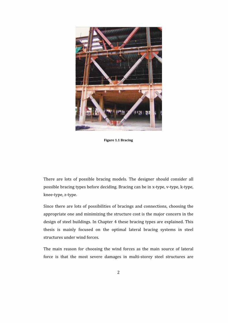
Sample bracing for a structure can be seen in Figure 1.1.

2

Figure 1.1 Bracing

There are lots of possible bracing models. The designer should consider all

possible bracing types before deciding. Bracing can be in x-type, v-type, k-type,

knee-type, z-type.

Since there are lots of possibilities of bracings and connections, choosing the

appropriate one and minimizing the structure cost is the major concern in the

design of steel buildings. In Chapter 4 these bracing types are explained. This

thesis is mainly focused on the optimal lateral bracing systems in steel

structures under wind forces.

The main reason for choosing the wind forces as the main source of lateral

force is that the most severe damages in multi-storey steel structures are

3

caused by winds. For example, in the United States between 1986 and 1993,

hurricanes and tornadoes caused $41 billion in insured catastrophic losses,

compared with $6.18 billion for all other natural hazards combined (Taranath,

Wind and Earthquake Resistant Buildings, 2005). In Chapter 3 detailed

descriptions of the wind loads are given. Calculation of the wind loads on

structures according to ASCE 7-05 is also explained in the chapter.

The optimization process is carried by a method called evolution strategies,

which is a member of the evolutionary algorithms search techniques. Evolution

strategies were developed in the early 1960s by Rechenberg and Schwefel, who

were working at the Technical University of Berlin on an application

concerning shape optimization (Eiben & Smith, 1998).

In the latter chapters descriptions of evolutionary algorithms, evolution

strategies, wind loads and bracing systems will be given.

1.1 Previous Studies

Another publication related with this topic is Memari & Madhkhan (1999),

which deals with the optimization of structures under seismic. Allowable stress

design of two-dimensional braced and unbraced steel frames based on AISC

specifications subject to gravity and seismic lateral forces is formulated as a

structural optimization problem. The objective function is the weight of the

structure, and behavior constraints include combined bending and axial stress,

shear stress, buckling, slenderness and drift. Cross-sectional areas are used as

design variables. Among the specific observations resulting from the examples

given in this study is insight with respect to the superiority of the K-braces over

the other types in a minimum weight design sense.

One publication is Kameshki & Saka (2001), which uses genetic algorithm for

the optimum design of bracing. In this study, the serviceability and stress

constraints given in BS 5950 (1990) is used. The algorithm is used to design tall

frames with bracings such as X, V and Z bracing. The main difference from our

4

study is that the frames were planar. The technique allows members grouping

and selects the required steel sections for beams, columns and bracing

members from a set of standard steel sections. The frame used for the

optimization procedure is three-bay, 15-storey frame. It is shown that X-

bracing system with pinned beam-column connections produces lightest frame.

In Pavlovcic, Krajnc, & Beg (2004) cost function analysis in the structural

optimization of steel frames is presented. It is outlined that generally the

fabrication and erection costs of the structures are disregarded. The minimum

weight does not always mean the most economical solution in the structural

design. Therefore, they developed a cost function for the steel frames and this

includes all essential fabrication and erection activities. It considers both

manufacturing costs as well as material costs. It is formulated in an open

manner, offering users to define their own parameters on the basis of a certain

production line.

In Hasançebi (2008) the computational performance of adaptive ESs in large-

scale structural optimization is mainly investigated to achieve following

objectives:

- To present an ESs based solution algorithm for efficient optimum design

of large structural systems consisting of continuous, discrete and mixed

design variables.

- To integrate new parameters and methodologies into adaptive ESs to

improve the computational performance of the algorithm.

- to assess successful self-adaptation models of ESs in continuous and

discrete structural optimizations

Two numerical examples are studied in depth to verify the enhanced

performance of the algorithm, as well as to scrutinize the role and significance

of self-adaptation in ESs for a successfully implemented optimization process.

The conclusions of the study are: (i) continuous optimization problems are best

handled using = , and = 1 should be avoided due to its deficient self-

5

adaptation capability, (ii) for discrete optimization problems the learning

process works better, if the algorithm is implemented with = 1, (iii) the

utilization of and parameters is crucial for a successfully implemented

optimization process, and greatly improves the convergence velocity of the

algorithm (iv) a remarkable increase in the efficiency of the algorithm can be

gained through the adaptive penalty function implementation.

1.2 Optimization of Steel Frames

In structural design process, there are lots of parameters affecting the design.

These are; past experience, tests, research, engineer’s capability etc. So for a

specific building there is not a single design. Every engineer can design the

building in a different way.

The designer makes the initial design, analyzes the building and decides if the

building is safe or not. If it is safe enough, he/she can search for a way to design

the structure in a more economical way. So the design process is somewhat a

trial and error process and every step takes considerable time. The need for the

computer software and optimization techniques arises from this aspect.

So when we use a computer with frame optimization software, we have these

advantages:

- We design more economical structures.

- We eliminate the designers that have less design experience since any

non-experienced engineer can make good designs by using structural

optimization software.

- We gain considerable amount of time since we use computers as a

computational source.

Therefore design optimization is a very important task. Because of that, it gains

attention and more designers make use of optimization in their works.

6

1.3 Evolutionary Algorithms

Evolutionary algorithms (EAs) are search methods that are inspired from

natural selection and survival of the fittest of the nature. EAs are different from

more traditional optimization techniques because they search the design space

using a population of solutions, not a single point. At every iteration of an EA,

the poor solutions are eliminated. The solutions having high fitness values are

recombined with other solutions that have high fitness by interchanging their

parts. These solutions are also mutated by making some changes to their

elements. To generate new solutions recombination and mutation are used, and

it is hoped that these new solutions move towards regions where the good

solutions lie. A brief flowchart for an EA is as follows:

- Initialize the population

- Evaluate initial population

- Apply genetic operators to generate new solutions

- Evaluate solutions in the population

- Perform competitive selection

- Repeat, above three steps, until some convergence criteria is satisfied

This process is iterated until a specified criterion is reached or until a solution

that meets the sufficient quality is found.

There are different types of EAs. The major ones are:

- Genetic Algorithms(GAs)

- Evolutionary Programming(EP)

- Evolution Strategies(ESs)

GAs were developed by Holland (University of Michigan) in the early 1960s. In

GAs, the solution of a problem is encoded in the form of strings of numbers

(traditionally binary). Both mutation and recombination are used in GAs and

the evaluation is made by using a fitness function.

7

EP was developed by Fogel first. Intelligent behavior was viewed as the ability

to predict the next state of the machine environment. When an input symbol is

presented to the machine, the machine generates an output symbol, which is

compared to the next input symbol. The current output symbol represents a

prediction of the next input symbol. The quality of the prediction is measured

by using a payoff function (Dumitrescu, Lazzerini, Jain, & Dumitrescu, 2000).

ESs were first developed by Rechenberg (1965) and Schwefel (1981). ESs use

natural representation with a vector of real values and main operators are

mutation, recombination and selection. The operators are applied in a loop. An

iteration of the loop is called a generation. The sequence of generations is

continued until a termination criterion is met. Since ESs are used in this study,

the brief introduction about ESs will be given in the next section.

1.4 Evolution Strategies

ESs are a branch of direct search and optimization methods that are inspired

from the nature, belonging to the class of EAs. ESs use natural problem-

dependent representations, and primarily mutation and selection as search

operators. The operators are applied in a loop. One iteration of the loop is

called a generation. The loops are continued until a termination criterion is

met.

It was created in the early 1960s by Rechenberg Schwefel at the Technical

University of Berlin, Germany.

At first, ESs were used for solving optimization problems related with fluid

dynamics, but later, they were used for solving other optimization problems

with discrete variables. As far as the search space is real valued, mutation is

normally applied by adding a normally distributed random value to each vector

component.

8

The simplest form of the EAs is the (1+1)-ES. In this form the individual creates

an offspring and if the offspring’s fitness is better or equal than the parent, it

becomes the parent of the next generation. Otherwise the offspring is

eliminated. The first multi-membered ES is the ( + 1)-ES. In this form

parents combine to generate a single offspring and this offsprings replaces the

worst parent.

These types are replaced by ( , )-ES and ( + )-ES. Here, stands for the

parents and stands for the offsprings. From -parents, -offsprings are

created and these offsprings compete with themselves in ( , )-ES, i.e. the

parents are eliminated. In ( + )-ES however, the parents are not eliminated

so both offsprings and the parents are in a competition. In Bäck (1996),

detailed explanations of these selection types and their drawbacks are given.

1.5 Aim and Scope of the Study

The main aim of this thesis is to investigate the effect of bracing system on

optimum design of steel structures. Different structures with different bracing

systems are sited for minimum weight and cost and the results are compared.

The thesis is organized as follows:

In Chapter 2 design optimization of steel frames using evolution strategies is

described. First detailed overview of the optimization subject is given. The

elements of the optimizations are mentioned and their details are also given in

this chapter. After that the design optimization of steel frames is formulated.

Optimization of a steel frame according to ASD-AISC is explained here. The

constraints such as stress, displacement, and geometry are formulated and

values of them are given. After defining the problem formulation the

evolutionary algorithms are introduced. The background information of them

and their main elements can be found here. Evolution strategies, being a

technique of evolutionary algorithms, are explained then. The background

information, different extensions and elements of ESs are given.

9

Chapter 3 focuses on the design loads on structures. There are four types of

loads on our structures. These are dead loads, live loads, snow loads and wind

loads. First a brief introduction about the wind loads is given and then the

calculation of wind loads on structures according to the ASCE 7-05 is outlined.

Then calculation of the other three load types is given then.

Chapter 4 discusses the bracing of steel frames. The advantages of bracing on

structures are emphasized and different types of bracing systems are given.

The illustrations of the bracing systems that are used in our structures are also

available in this chapter.

Chapter 5 is the cost analysis of steel frames. The cost of our structures is

mainly assumed to be composed of four elements. These are, cost of elements,

cost of joints, cost of transportation and cost of erection. In this chapter the

calculation of the cost of a structure is outlined.

In Chapter 6, numerical examples are given. Details of the test problems for the

optimum bracing type are explained. There are three different structures. They

have 10, 20 and 30 floors respectively. Different bracing types are applied to

these structures and optimum designs of them are carried out.

Chapter 7 gives interpretation of the results obtained. The comparison of the

bracing types and their behaviors are described here.

Chapter 8 makes a conclusion of the thesis by outlining the results and

discussions.

10

Chapter 2

OPTIMUM DESIGN OF STEEL FRAMES USING

EVOLUTION STRATEGIES

2.1 Optimization

Optimization can be described as the process of having the best solution of a

given objective(s) while satisfying certain restrictions. It can also be defined as

finding the minima or maxima of a given objective function under some

constraints.

Being a very widely used phenomenon in today’s world, optimization is used to

improve business processes in practically all industries such as operations

research, artificial intelligence, computer science, and structural design.

There are mainly four elements of optimization. These are:

- Design variables

- Constraints

- Objective function

- Design space

11

In order to improve a property of a structure, one has to change some

parameters of it. These parameters are called design variables. Design variables

can be a cross-sectional dimension or simply be a cross-section type from a

given set of steel sections. Design variables can take either discrete or

continuous values. For instance in case of having a set of steel sections that we

can purchase from, we need to use discrete design variables. If we want the

variable to assume any value between some boundaries, then we use

continuous design variables. Some design variables can also be set to some

specific values that are not to be changed during the design process. These

parameters are called preassigned parameters.

Constraints are some special conditions that the design must satisfy in order to

be accepted as a feasible design. This can be the cross-sectional dimensions of a

column to be in a range or a stress in a member not to exceed a given value.

There are two different constraint types. These are geometric constraints and

behavior constraints. The need for a geometric constraint may arise from

fabrication limitations or aesthetics. A typical example for a behavior constraint

is the strength of a member.

Objective functions are the functions that measure the quality of the design.

Different solutions are compared according to their objective functions. For

structural optimization, minimization of cost, weight, displacement, stress or

load can be used as objective function. If the problem has a single objective

function, it said to be a single-criterion optimization problem. If it has multiple

objective functions, it is a multi-criteria optimization problem.

There are mainly three types of structural optimization. These are size

optimization, shape (geometry) optimization and topology optimization.

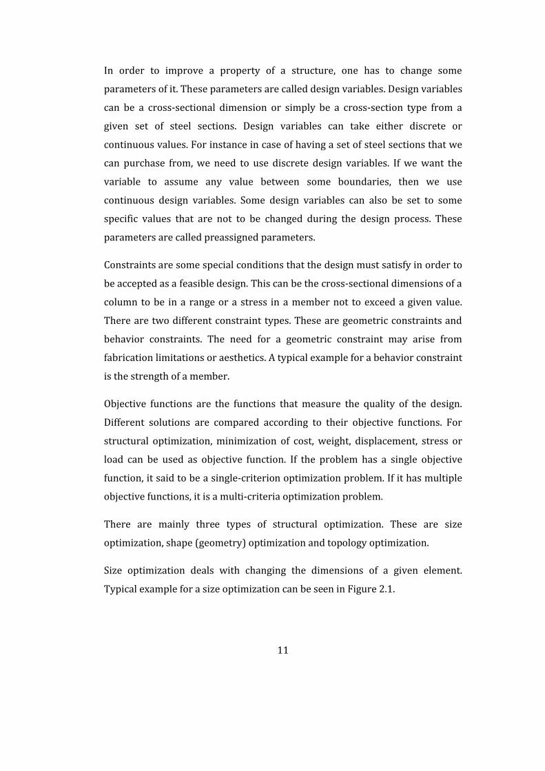
Size optimization deals with changing the dimensions of a given element.

Typical example for a size optimization can be seen in Figure 2.1.

12

Shape optimization deals with changing the shape of the element, such that

optimum locations of nodes in a finite element model of the structure are

determined.

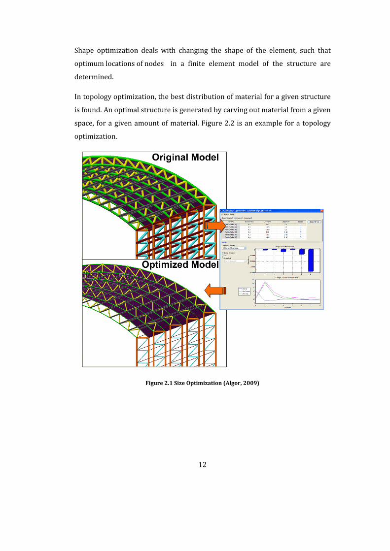
In topology optimization, the best distribution of material for a given structure

is found. An optimal structure is generated by carving out material from a given

space, for a given amount of material. Figure 2.2 is an example for a topology

optimization.

Figure 2.1 Size Optimization (Algor, 2009)

13

Figure 2.2 Topology Optimization Example (Topologica Solutions, 2009)

2.2 Design Optimization of Steel Frames

For a steel frame structure consisting of mN members that are collected in dN

design groups (variables), the optimum design problem according to

AISC(1989) code yields the following discrete programming problem, if the

design groups are selected from steel sections in a given profile list.

Find a vector of integer values I (Equation (2-1)) representing the sequence

numbers of steel sections assigned to member groups

= , , … , (2-1)

to minimize the weight (W ) of the frame:

14

td N

jj

N

iii LAW

11

(2-2)

where iA and i are the length and unit weight of the steel section adopted for

member group i, respectively, tN is the total number of members in group i,

and jL is the length of the member j which belongs to group i.

The members subjected to a combination of axial compression and flexural

stress must be sized to meet the following stress constraints:

> 0.15;⎣⎢⎢⎢⎡

+ 1 − ′+ 1 − ′ ⎦⎥

⎥⎥⎤

− 1.0 ≤ 0 (2-3)

0.6 + + − 1.0 ≤ 0 (2-4)

≤ 0.15; + + − 1.0 ≤ 0 (2-5)

If the flexural member is under tension, then the following formula is used

instead:

0.6 + + − 1.0 ≤ 0 (2-6)

In Equations (2-3) to (2-6):

15

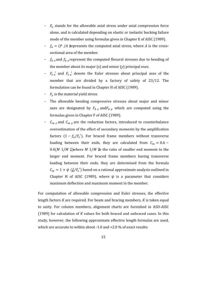
- stands for the allowable axial stress under axial compression force

alone, and is calculated depending on elastic or inelastic bucking failure

mode of the member using formulas given in Chapter E of AISC (1989).

- = ( / )represents the computed axial stress, where A is the cross-

sectional area of the member.

- and represent the computed flexural stresses due to bending of

the member about its major (x) and minor (y) principal exes.

- ′ and ′ denote the Euler stresses about principal axes of the

member that are divided by a factory of safety of 23/12. The

formulation can be found in Chapter H of AISC (1989).

- is the material yield stress

- The allowable bending compressive stresses about major and minor

axes are designated by and , which are computed using the

formulas given in Chapter F of AISC (1989).

- and are the reduction factors, introduced to counterbalance

overestimation of the effect of secondary moments by the amplification

factors (1 − / ′). For braced frame members without transverse

loading between their ends, they are calculated from = 0.6 −0.4( 1/ 2), where 1/ 2is the ratio of smaller end moment to the

larger end moment. For braced frame members having transverse

loading between their ends, they are determined from the formula

= 1 + ( / ′) based on a rational approximate analysis outlined in

Chapter H of AISC (1989), where is a parameter that considers

maximum deflection and maximum moment in the member.

For computation of allowable compression and Euler stresses, the effective

length factors K are required. For beam and bracing members, K is taken equal

to unity. For column members, alignment charts are furnished in ASD-AISC

(1989) for calculation of K values for both braced and unbraced cases. In this

study, however, the following approximate effective length formulas are used,

which are accurate to within about -1.0 and +2.0 % of exact results:

16

For unbraced members:

= 1.6 + 4( + ) + 7.5+ + 7.5 (2-7)

For braced members:

= 3 + 1.4( + ) + 0.643 + 2.0( + ) + 1.28 (2-8)

Where and refer to stiffness ratio or relative stiffness of a column at its

two ends.

It is also required that computed shear stresses ( ) in members are smaller

than allowable shear stresses ( ), as formulated in Equation (2-9).

≤ = 0.40 (2-9)

In Equation (2-9), is referred to as web shear coefficient. It is taken equal to

= 1.0 for rolled W-shaped members with ℎ/ ≤ 2.24 / , where ℎ is the

clear distance between flanges, is the elasticity modulus and is the

thickness of web. For all other symmetric shapes, is calculated from

formulas given in Chapter G of ANSI/AISC (2005).

Apart from stress constraints, slenderness limitations are also imposed on all

members such that maximum slenderness ratio ( = / )is limited to 300

for members under tension, and to 200 for members under compression loads.

The displacement constraints are imposed such that the maximum lateral

displacements are restricted to be less than /400, and upper limit of story

drift is set to be ℎ/400, where is the total height of the frame building and ℎis the height of a story.

17

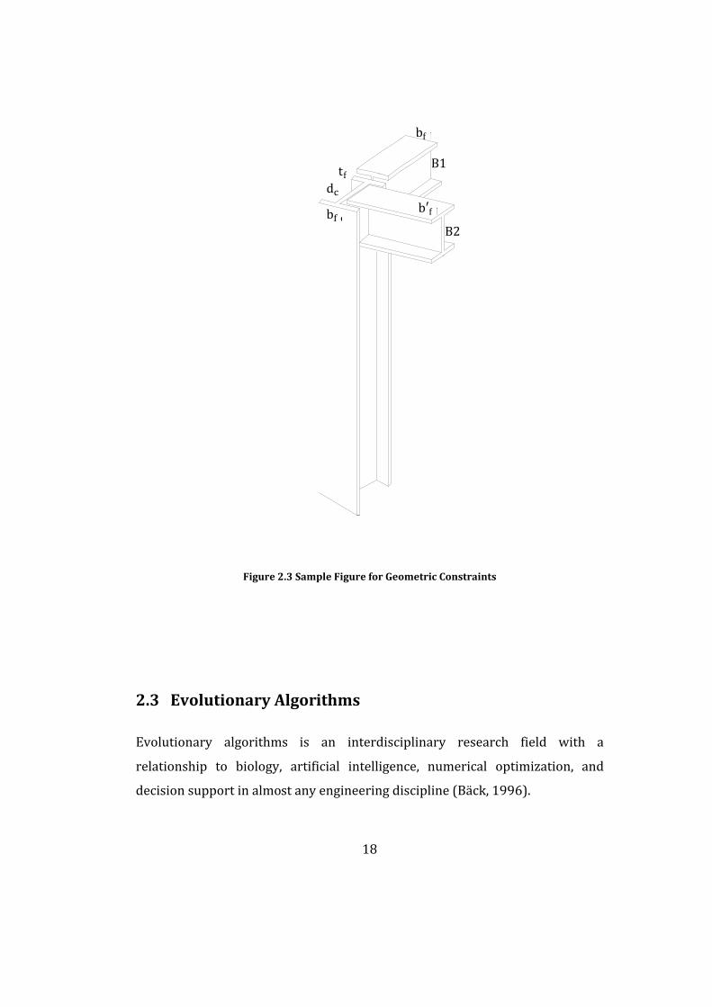
Finally, we consider geometric constraints between beams and columns

framing into each other at a common joint for practicality of an optimum

solution generated. For the two beams B1 and B2 and the column shown in

Figure 2.3, one can write the following geometric constraints:

− 1.0 ≤ 0 (2-10)

′( − 2 ) − 1.0 ≤ 0 (2-11)

where , ′ and are the flange width of the beam B1, the beam B2 and

the column, respectively, is the depth of the column, and is the flange

width of the column. Equation (2-10) simply ensures that the flange width of

the beam B1 remains smaller than that of the column. On the other hand,

Equation (2-11) enables that flange width of the beam B2 remains smaller than

clear distance between the flanges of the column( − 2 ).

18

Figure 2.3 Sample Figure for Geometric Constraints

2.3 Evolutionary Algorithms

Evolutionary algorithms is an interdisciplinary research field with a

relationship to biology, artificial intelligence, numerical optimization, and

decision support in almost any engineering discipline (Bäck, 1996).

B1

b

b′B2

tdb

19

There are lots of possible techniques of evolutionary algorithms. The common

underlying idea behind all is the same: given a population of individuals, the

environmental pressure causes natural selection (survival of the fittest), which

causes a rise in the fitness of the population. Given a quality function to be

maximized, we can randomly create a set of candidate solutions, i.e., elements

of the function’s domain, and apply the quality function as an abstract fitness

measure – the higher the better. Based on this fitness, some of the better

candidates are chosen to seed the next generation by applying recombination

and/or mutation to them. Recombination is an operator applied to two or more

selected candidates (the so-called parents) and results one or more new

candidates (the children). Mutation is applied to one candidate and results in

one new candidate. Executing recombination and mutation leads to a set of new

candidates (the offspring) that compete – based on their fitness (and possibly

age) – with the old ones for a place in the next generation. This process can be

iterated until a candidate with sufficient quality (a solution) is found or

previously set computational limit is reached (Eiben & Smith, 1998) .

In evolutionary algorithms there are two fundamental forces:

- Variant Operators: Recombination and Mutation.

- Selection: It is the force that pushes quality.

In evolutionary algorithms, although the weak individuals have a chance to be

selected as a parent, fitter individuals have a higher chance to be selected.

Evolutionary Algorithms have various elements such as:

- Representation

- Evaluation Function

- Population

- Parent Selection Mechanism

- Variation operators; recombination and mutation

- Survivor Selection Mechanism

20

This process is used by different techniques, i.e. evolution strategies, genetic

algorithms and evolutionary programming. In the next section evolution

strategies will be explained.

2.4 Evolution Strategies

The fundamentals of ESs were originally laid in the pioneering studies of

Rechenberg (1965, 1973) and Schwefel (1965) at the Technical University of

Berlin. They developed the first (simplest) variant of ESs, which implements on

the basis of two designs; a parent and an offspring individual. Today, the

modern variants of ESs are accepted as ( + ) − and ( , ) − , which

were again developed by Schwefel (1977, 1981). Both variants employ design

populations consisting of parent and offspring individuals, and are intended

to carry out a self-adaptive search in continuous design spaces. The extensions

of these variants to solve discrete optimization problems were put forward in

the following three studies in the literature: Cai and Thierauf (1993), Bäck and

Schütz (1995), and Rudolph (1994). Amongst them, the one proposed by Cai

and Thierauf (1993) refers to a non-adaptive reformulation of the technique

and has probably found the most applications in discrete structural

optimization. The approach proposed by Bäck and Schütz (1995) corresponds

to an adaptive reformulation of the technique, which incorporates a self-

adaptive strategy parameter called mutation probability. Another adaptive

reformulation of ESs is presented by Rudolph (1994) for general non-linear

mathematical optimization problems.

2.4.1 Optimization Routine

As in all EA techniques, the underlying idea of ESs rests on simulation of natural

evolution in an effort to evolve a population of individuals (designs) towards

the optimum. In this framework, both continuous and discrete adaptive ESs

make use of a common optimization routine featuring a generation-based

iteration of the technique. This routine is outlined in the flowchart shown in

21

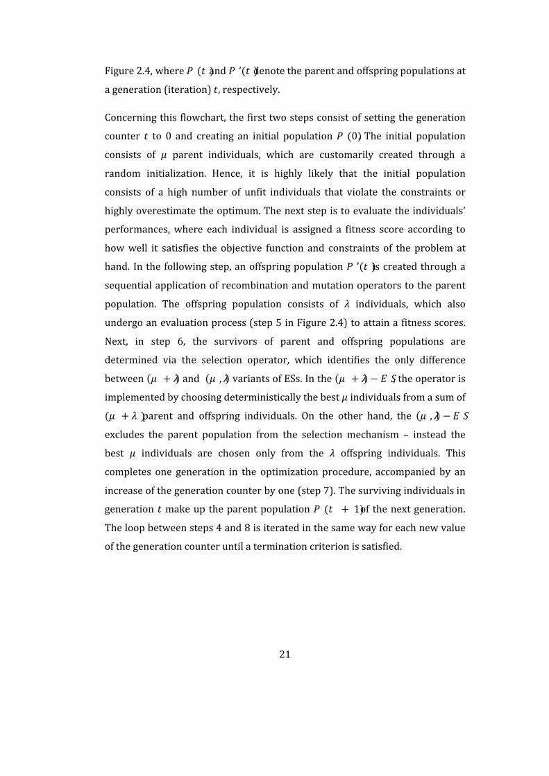
Figure 2.4, where ( )and ’( )denote the parent and offspring populations at

a generation (iteration) , respectively.

Concerning this flowchart, the first two steps consist of setting the generation

counter to 0 and creating an initial population (0). The initial population

consists of parent individuals, which are customarily created through a

random initialization. Hence, it is highly likely that the initial population

consists of a high number of unfit individuals that violate the constraints or

highly overestimate the optimum. The next step is to evaluate the individuals’

performances, where each individual is assigned a fitness score according to

how well it satisfies the objective function and constraints of the problem at

hand. In the following step, an offspring population ’( )is created through a

sequential application of recombination and mutation operators to the parent

population. The offspring population consists of individuals, which also

undergo an evaluation process (step 5 in Figure 2.4) to attain a fitness scores.

Next, in step 6, the survivors of parent and offspring populations are

determined via the selection operator, which identifies the only difference

between ( + ) and ( , ) variants of ESs. In the ( + ) − , the operator is

implemented by choosing deterministically the best individuals from a sum of

( + )parent and offspring individuals. On the other hand, the ( , ) −excludes the parent population from the selection mechanism – instead the

best individuals are chosen only from the offspring individuals. This

completes one generation in the optimization procedure, accompanied by an

increase of the generation counter by one (step 7). The surviving individuals in

generation make up the parent population ( + 1)of the next generation.

The loop between steps 4 and 8 is iterated in the same way for each new value

of the generation counter until a termination criterion is satisfied.

22

Figure 2.4 Optimization Routine

The optimization routine discussed above forms the basic framework

of the solution algorithm developed in the present work.

(+)

Begin the process

Step 1: t := 0; Set the generation counter to 0

Step 2: initialize P (0); Create an initial population with parent individuals

Step 3: evaluate P (0); Evaluate the initial population P (0)

Step 4: P’ (t ):=recom and mut P (t );Create an offspring population with individuals by recombining and mutating the parent population

Step 5: evaluate P’ (t ); Evaluate the offspring population

Step 6: selectionP (t +1):=select from (P (t ) and P’ (t )); Select the best individuals from both parent and offspring populations

P (t +1):=select from P’ (t ); Select the best individuals from offspring population only

Terminate the process

Step 7: t := t + 1; Increase generation counter by one

Step 8:if termination criterion is

satisfied?

( ,)

YES

NO

23

2.4.2 ESs for Continuous Variables

In this section ( , )-ES formulation for problems having continuous design

variables will be given.

2.4.2.1 Representation of an Individual and Initial

Population

As the most general form of individuals in ESs, the Equation (2-12) can be used:

= ( , , ) (2-12)

Where represents the individual (a possible solution) in ESs. It consists of

three components, , and . represents the design variables vector and it is

used to calculate the objective function. and represents the strategy

parameter set of .Search points in Evolution Strategies are n-dimensional object parameter

vectors ℝ. The objective function Φ is in principle identical to the fitness

function: ℝ → ℝ , i.e. given an individual , we have;

Φ( ) = ( ) (2-13)

Where is the object variable component of =( , , ) = ℝ× , where;

24

= ℝ × [− , ] (2-14)

{1, … , } (2-15)

{0, (2 − )( − 1)/2} (2-16)

Besides representing the object variable vector , each individual may

additionally include one up to different standard deviations as well as up to

∙ ( − 1)/2(namely when = ) rotation angles [− , ] ( {1, … , −1}, { + 1, … , }), such that the maximum number of strategy parameters

amounts to = ∙ ( + 1)/2. For the case 1 < < , the standard deviations

σ , … , σ are coupled with object variables x , … , x and σ is used for

the remaining variables x , … , x . Here is the size of the vector of object

variables.

The number of rotation angles depends directly on , the number of

standard deviations, and , but it can also explicitly be set to zero, indicating

that this strategy parameter part of individuals is not used (Bäck, 1996).

Initial population consisting of parent individuals is created by means of a

random initialization. Therefore, for each individual the variables are selected

with a uniform distribution between their specified lower and upper bounds.

No requirement regarding the feasibility of the individuals is enforced, and thus

the initial population is permitted to retain infeasible individuals in addition to

feasible ones.

2.4.2.2 Constraint Handling and Evaluation of Population

Not only the objective function, but also the problem constraints have to be

taken into account during the evaluation process of parent and offspring

individuals. A variety of different approaches and/or specialized operators

have been proposed in the literature to handle constraints. The constraints are

25

dealt with using an external penalty function approach in this study. Objective

function values of the feasible solutions that satisfy all the problem constraints

are directly calculated first. Then the infeasible solutions that violate some of

the problem constraints are penalized using external penalty function

approach, and their objective function values are calculated according to:

Φ = Φ[1 + Penalty(a)] = Φ 1 + r g (2-17)

In Equation (2-17), Φ is the constrained objective function value. g , =1, . . , n represents the whole set of normalized constraints, and is the penalty

coefficient used to tune the intensity of penalization as a whole. Although r can

be assigned to an appropriate static value, such as = 1, an adaptive penalty

function implementation is favored by letting this parameter adjust its value

automatically during the search for the most efficient optimization process. The

second method (letting to adjust itself during search) can be made by:

( ) =⎩⎨⎧ 1 ∙ ( − 1) ( − 1)

∙ ( − 1) ( − 1) � (2-18)

Where ( )and ( − 1)denote the penalty coefficients at generations and

− 1, respectively, ( − 1)is the best design at generation − 1, and is an

arbitrary constant referred to as the learning rate parameter of . Experiments

with various test problems indicate that the optimal value of equals to 1.1.

The rationale behind Equation (2-18) is to continually enforce the algorithm to

adopt a search direction along the constraint boundaries. If the best individual

at the preceding generation is infeasible, the penalty is intensified somewhat in

order to render the feasible regions more attractive for individuals, and thereby

guiding the search towards these regions. If, however, the best individual at the

26

preceding generation is feasible, this time the search is directed towards

infeasible regions by relaxing the penalty to some extent. The overall

consequence of this action is that the search is carried out very close to

constraint boundaries throughout the optimization process. Another feature of

the adaptive penalty function is that it avoids entrapment of the search at local

optimum, which is the case, often observed when a static penalty function is

utilized.

2.4.2.3 Recombination

Recombination is applied to create an offspring population, such that µ parent

individuals undergo an exchange of design characteristics to produce

offspring individuals. Several recombination operators exist and, in principle,

recombination of different components of an individual can be implemented

using different operators. Assuming that represents an arbitrary component

of an individual, a formulation of these operators is given in Equation (2-19) as

applied to produce ′:

′ =

⎩⎪⎪⎪⎪⎨⎪⎪⎪⎪⎧ , ,

, , ,, ,,

, + , − ,2 ,, + ,− ,2 ,

� (2-19)

Where and represents the component of any two parent individuals

that are chosen from parent population at random:

- Type (1) corresponds to the no recombination case; ′ is simply formed

by duplicating .

27

- Type (2) is named as discrete recombination and each element of ′is

selected from one of the two parents ( ) under equal

probability.

- Type (3) is called as the global version of discrete recombination such

that the first parent is selected and held unchanged, while a second

parent is randomly determined anew for each element of , and then ′is chosen from one of these parents ( , ) under equal probability.

- Intermediate forms of type (2) and (3) are given in types (4) and (5),

respectively, which are identical to the former except that arithmetic

means of the elements are calculated.

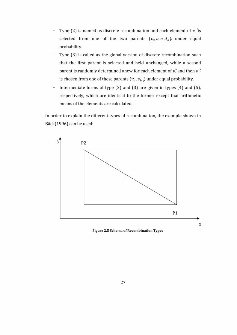
In order to explain the different types of recombination, the example shown in

Bäck(1996) can be used:

P2

P1

Figure 2.5 Schema of Recombination Types

x

y

28

In Figure 2.5 P1 and P2 represents the object variable points represented by

two parent individuals. Only the corners of the rectangle defined by P1 and P2

can be reached by means of discrete recombination (Type (2) and Type (3)).

Intermediate recombination (Type (4) and Type (5)) yields the center of the

rectangles’ diagonal lines.

2.4.2.4 Mutation

The mutation operator in ESs is based on a normal (Gaussian) distribution

requiring two parameters: the mean and the standard deviation .

In practice, the mean is always set to zero, and the vector is mutated by

replacing values by:

= + (0, ) (2-20)

where (0, )denotes a random number drawn from a Gaussian distribution

with zero mean and standard deviation . By using a Gaussian distribution

here, it is ensured that small mutations are more likely than larger ones.

What is important here is that the mutation step sizes are not set by the user;

rather the is coevolving with the solutions. In order to achieve this behavior it

is essential to modify the value of first, and then mutate the values with the

new value. The rationale behind this is that a new individual ( , ) is

effectively evaluated twice. Primarily, it is evaluated directly for its viability

during survivor selection based on ( ). Second, it is evaluated for its ability to

create good offspring. This happens indirectly: a given step size evaluates

favorably if the offspring generated by using it prove viable (in the first sense).

Thus, an individual ( , ′)represents both a good that survived selection

and a good ′that proved successful in generating this good from (Eiben &

Smith, 1998).

29

Since a general formulation of mutation is given in Equation (2-20), now the

three special cases of mutation can be given;

- Uncorrelated Mutation with One Step Size

- Uncorrelated Mutation with Step Sizes

- Correlated Mutation

2.4.2.4.1 Uncorrelated Mutation with One Step Size

In this case of mutation, the same distribution pattern is used to mutate the

values of . That means we have only one single value of the strategy parameter

for each individual. This type of mutation can be expressed as:

= ∙ exp ( ∙ (0,1)) (2-21)

= + ′ ∙ (0,1) (2-22)

Where (0,1)denotes the standard normal distribution, (0,1) denotes the

single standard normal distribution for each variable . The denotes the

proportionality constant. It can be explained as the learning rate. It is usually

inversely proportional with the square root of the problem size:

∝ 1/√ (2-23)

The values are required not to get close to zero, so a boundary condition is set

for the , and if it gets below that level, is set to that boundary value.

30

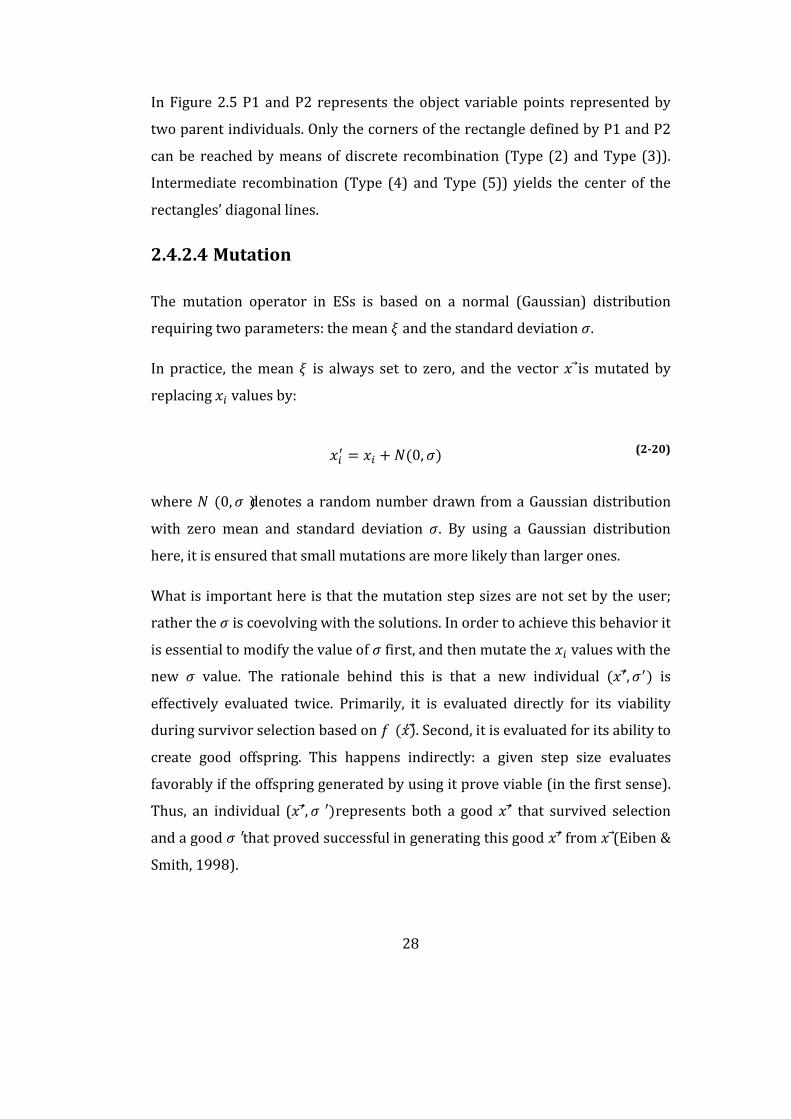
Let’s assume that we have a population with n=2 and this is an uncorrelated

mutation with one step size; n = 1, n = 0. In Figure 2.6 the black dot

represents the local maximum and the circle indicates the points where the

offsprings can be placed with a given probability. The probability of moving

along both the x-axis and y-axis are the same.

2.4.2.4.2 Uncorrelated Mutation with Step Sizes

In this case of mutation, the different distribution patterns are used to mutate

the values of . The reason for this is that the fitness directions can have

different slopes for different directions. That means we have different values of

the strategy parameter for each variable of an individual. This type of

mutation can be expressed as:

x

y

Figure 2.6 Uncorrelated Mutation With One Step Size

31

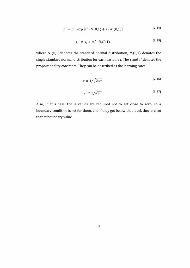
= ∙ exp [ ∙ (0,1) + ∙ (0,1)] (2-24)

= + ′ ∙ (0,1) (2-25)

where (0,1)denotes the standard normal distribution, (0,1) denotes the

single standard normal distribution for each variable . The and denotes the

proportionality constants. They can be described as the learning rate:

∝ 1/ 2√ (2-26)

′ ∝ 1/√2 (2-27)

Also, in this case, the values are required not to get close to zero, so a

boundary condition is set for them, and if they get below that level, they are set

to that boundary value.

32

y

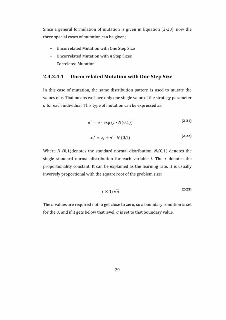
Let’s assume that we have a population with n=2 and since this is an

uncorrelated mutation with step sizes; n = n = 2, n = 0. In Figure 2.7 the

black dot represents the local maximum and the ellipse indicates the points

where the offsprings can be placed with a given probability. The probability of

moving along both the x-axis and y-axis are not the same. The probability of

moving along x-axis (large effect on fitness) is larger than the probability of

moving along the y-axis (small effect on fitness).

2.4.2.4.3 Correlated Mutations

In this case of mutation, the different distribution patterns are used to mutate

the values of and also the mutation has rotation angles. In the previous form

of mutation explained in 2.4.2.4.2 the shape of the search space is ellipse but it

was still orthogonal to the axes. This version allows the ellipse to have any

orientation by rotating it with rotation matrix . That means we have different

x

12

Figure 2.7 Uncorrelated Mutation With n Step Sizes

33

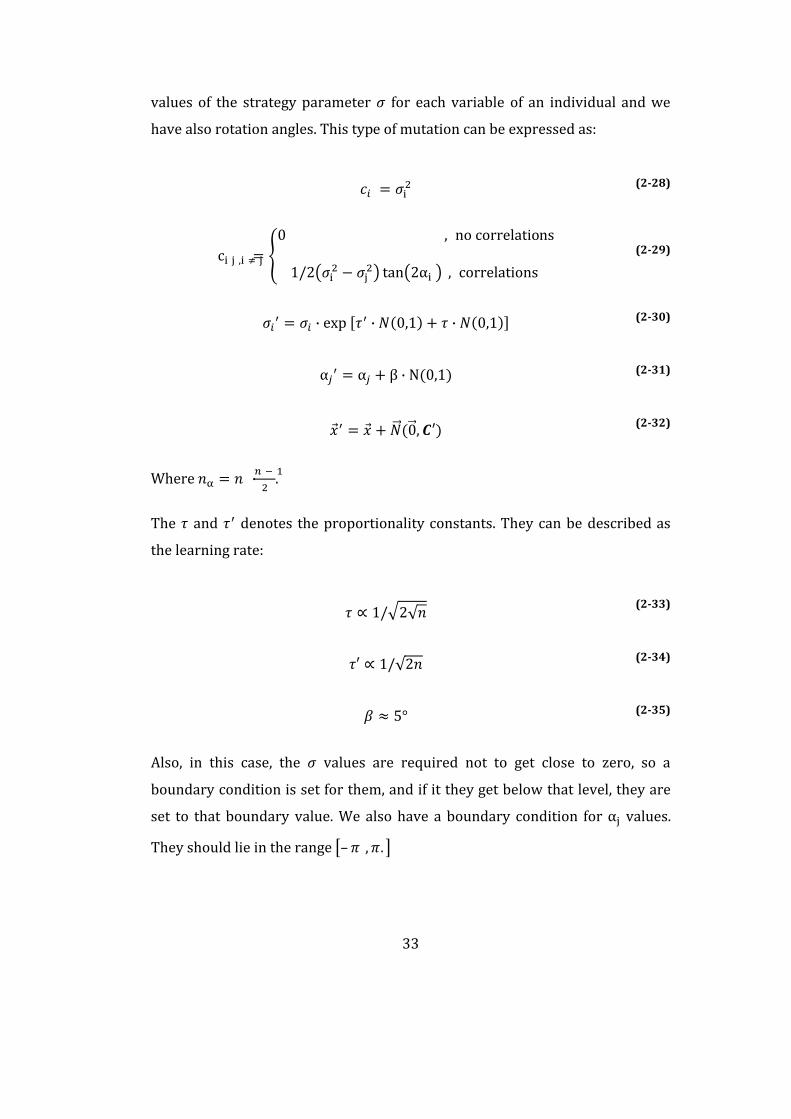
values of the strategy parameter for each variable of an individual and we

have also rotation angles. This type of mutation can be expressed as:

= (2-28)

c , = 0 , no correlations1/2 − tan 2α , correlations � (2-29)

= ∙ exp [ ∙ (0,1) + ∙ (0,1)] (2-30)

α = α + β ∙ N(0,1) (2-31)

= + (0, ′) (2-32)

Where = ∙ .

The and denotes the proportionality constants. They can be described as

the learning rate:

∝ 1/ 2√ (2-33)

′ ∝ 1/√2 (2-34)

≈ 5° (2-35)

Also, in this case, the values are required not to get close to zero, so a

boundary condition is set for them, and if it they get below that level, they are

set to that boundary value. We also have a boundary condition for α values.

They should lie in the range – , .

34

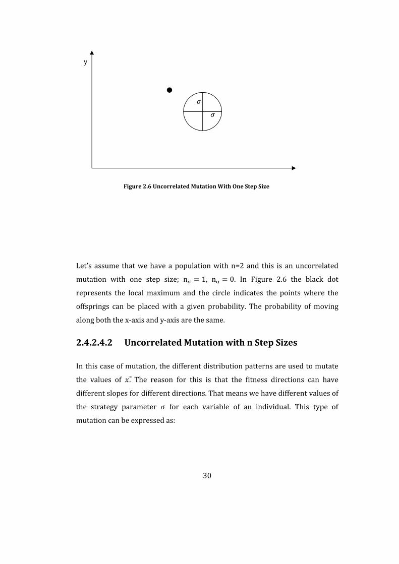
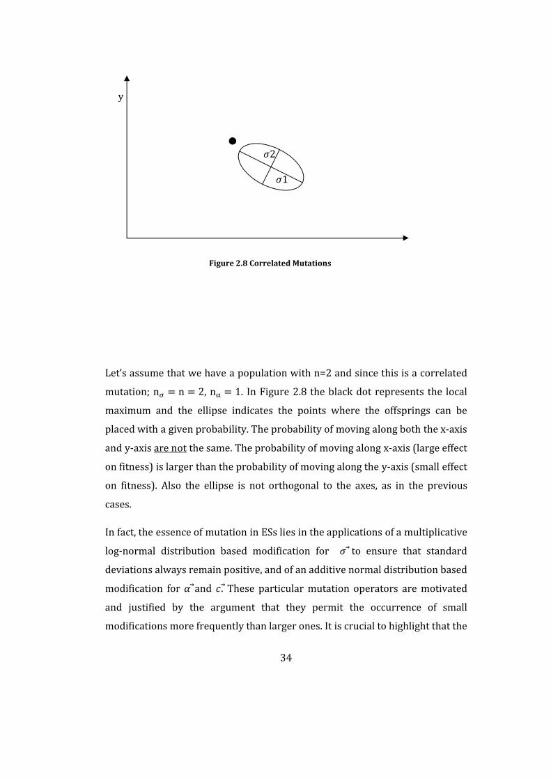
Let’s assume that we have a population with n=2 and since this is a correlated

mutation; n = n = 2, n = 1. In Figure 2.8 the black dot represents the local

maximum and the ellipse indicates the points where the offsprings can be

placed with a given probability. The probability of moving along both the x-axis

and y-axis are not the same. The probability of moving along x-axis (large effect

on fitness) is larger than the probability of moving along the y-axis (small effect

on fitness). Also the ellipse is not orthogonal to the axes, as in the previous

cases.

In fact, the essence of mutation in ESs lies in the applications of a multiplicative

log-normal distribution based modification for to ensure that standard

deviations always remain positive, and of an additive normal distribution based

modification for and . These particular mutation operators are motivated

and justified by the argument that they permit the occurrence of small

modifications more frequently than larger ones. It is crucial to highlight that the

x

12

Figure 2.8 Correlated Mutations

y

35

effectiveness and robustness of the mutation operator stem from the inherent

self-adaptation capability of the strategy parameters. The fact that the strategy

parameters are allowed to evolve together with the design variables during the

course of optimization, improves convergence rate and reliability of the

algorithm. For example, standard deviations attain large and small values from

time-to-time to avoid entrapment in a local optimum in the former, and to

accomplish a more exploitative search in the latter. Likewise, rotation angles

are automatically adjusted to suitable values to determine the optimal search

direction.

2.4.2.5 Selection

Selection is implemented next to determine the survivors out of parent and

offspring populations. There are ),( and )( type of selection strategy

in ESs. In ),( selection, the parents are all left to die out, and the best

offspring having the lowest objective function scores are selected

deterministically out of offspring. In )( selection, the selection is made

among both parents and offsprings. The selected (surviving) individuals

become the parents of the next generation.

The ),( -selection is preferred more because of the following reasons:

- The ),( discards all parents and is therefore in principle able to leave

small local optima, so it is advantageous in the case of multimodal

topologies.

- If the fitness function is not fixed, but changes in time, the )(

selection preserves outdated solutions, so it is not able to follow the

moving optimum well.

- )( selection hinders the self-adaptation mechanism with respect

to strategy parameters to work effectively, because maladapted strategy

parameters may survive for a relatively large number of generations

36

when an individual has relatively good object variables and bad strategy

parameters. In that case often all its children will be bad, so with elitism,

the bad strategy parameters may survive(Eiben & Smith, 1998).

Therefore, the ( , )-ESs is recommended. Investigations from a particular

objective function indicating a ratio of = 1/7 is optimal, concerning the

accelerating effect of self-adaptation (but has to be chosen clearly larger than

one, e.g. = 15)(Bäck, 1996).

2.4.2.6 Termination

The algorithm terminates when a pre-assigned parameter, such as the

generation number, pre-assigned time or sufficient convergence is reached, and

the best individual sampled thus far is regarded to be the optimum solution.

2.4.3 ESs for Discrete Variables

As stated previously, the three extensions of ESs to solve discrete optimization

problems were proposed by Cai and Thierauf (1993), Bäck and Schütz (1995),

and Rudolph (1994). They all employ the general optimization routine of

( + )and ( , )variants of ESs, and differ from each other in terms of the

application of mutation only. In our study a refined version of the Rudolph’s

approach is used, resulting in an increased performance of the approach. This

particular approach will be described in latter sections.

2.4.3.1 Representation of an Individual and Initial

Population

Initial population consists of number of parent solutions (individuals). As a

usual procedure in any EA technique, a random initialization of design variable

vectors is implemented for this purpose. That is, for each variable, a steel

section is assigned arbitrarily from the associated discrete set. Apart from the

37

vector of design variables , each individual comprises strategy parameters,

Equation (2-36). Both strategy parameters are self-adaptive by nature, and are

employed by the individual for establishing a problem-specific search scheme

in an automated manner.

= ( , ) (2-36)

In Equation (2-36) stands for the design vector, corresponding to that

component of the individual where the information related to number of

independent design variables is stored. The second component represents the

set of strategy parameters employed by the individual for establishing an

automated problem-specific search mechanism in exploring the design space.

A random initialization of population is implemented for the design vectors,

and the strategy parameters are assigned to appropriate values initially based

on numerical experimentation.

2.4.3.2 Constraint Handling and Evaluation of Population

Constraint handling and evaluation of population of ESs having discrete

variables are identical to discrete ESs. It is described in section 2.4.2.2.

2.4.3.3 Recombination

After evaluated, the parent population undergoes recombination and mutation

operators to yield the offspring population. Recombination provides a trade of

design information between the parents to generate new individuals

(offsprings). Recombination can be applied not only to design vectors, but also

to the strategy parameters of the individuals in a variety of different schemes.

In the present study a global discrete recombination operator is utilized for

design variables, whereas strategy parameters are recombined using

38

intermediate scheme. Given that represents an arbitrary component of an

individual, the recombined ′can be formulated as follows:

′ = , + ( − )/2,

� (2-37)

Where and refer to the component of two parent individuals which are

chosen randomly from the parent population, and and represent typical

elements of and . In global discrete recombination, is chosen from the

two parents under equal probability such that the first parent is held

unchanged, whereas the second parent is chosen a new for each element of i . In

intermediate recombination scheme, both parents are kept fixed for all

elements of i and their arithmetic means are calculated.

2.4.3.4 Mutation

Every offspring individual is subjected to mutation, resulting in a new set of

values for the design variables ( ′) and strategy parameters ( ′) of the

individual, Equation (2-38). This implies that not only the design information,

but also the search strategy of the individual is altered during this process.

( , ) = ′( ′, ′) (2-38)

As a general procedure, mutation of the strategy parameters is performed first.

The mutated values of the strategy parameters are then used to mutate the

design vector. Mutation of the design vector causes the individual to move to a

new point within the design space, and can be formulated as follows:

39

= + (2-39)

Where =[ , … , , … , ] refers to an n-dimensional random vector. The

mutated design vector ′ =[ ′, … , ′, … , ′] is simply obtained by adding this

random vector to the un-mutated design vector .

As far as discrete size optimum design of structures is concerned, design

variables correspond to cross-sectional areas of the structural members, which

are chosen from ready sections in a given profile list. To identify different

sections in a profile list, each section is indicated with a separate index number

between 1 and , where denotes the total number of ready sections in the

profile list. It is essential to highlight that the application of mutation for these

problems is actually performed using these indexes. That is to say, a design

variable initially corresponding to -th ready section of the profile list is

assigned to + -th section, after Equation (2-39) is performed.

2.4.3.4.1 Mutation Approach Proposed By Rudolph

Rudolph developed an adaptive reformulation of ESs for solving general non-

linear mathematical optimization problems with unbounded integer design

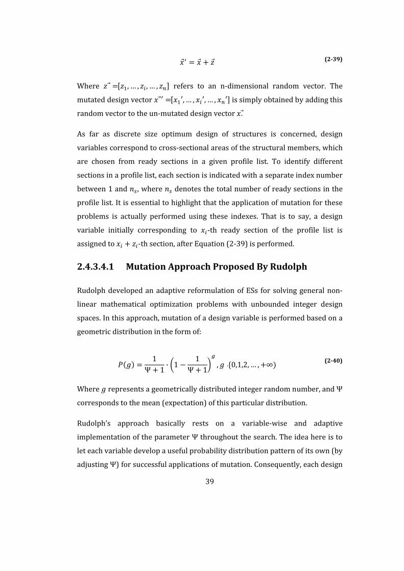
spaces. In this approach, mutation of a design variable is performed based on a

geometric distribution in the form of:

( ) = 1Ψ + 1 ∙ 1 − 1Ψ + 1 , {0,1,2, … , +∞) (2-40)

Where represents a geometrically distributed integer random number, and Ψcorresponds to the mean (expectation) of this particular distribution.

Rudolph’s approach basically rests on a variable-wise and adaptive

implementation of the parameter Ψ throughout the search. The idea here is to

let each variable develop a useful probability distribution pattern of its own (by

adjusting Ψ) for successful applications of mutation. Consequently, each design

40

variable of an individual is coupled with a different Ψ , {1,2, … , }parameter, and the individual is described as follows:

= ( , Ψ ) (2-41)

According to Rudolph’s approach, all design variables of an individual are

subjected to mutation. When interpreted in view of discrete function

optimization in mathematics, this strategy is plausible, as it causes an n-

dimensional mutation of the individual to a next grid point in the vicinity of the

former. However, structural optimization problems are such that the overall

behavior of a structural system might be very sensitive to changes in a few

design variables owing to significant variations in the properties of ready

sections. For a successful operation of mutation for these problems, it is

essential to limit the number of design variables mutated at a time in an

individual, as practiced by the former approaches. To this end, a refinement of

Rudolph’s approach is accomplished here, where the parameter is

incorporated and coupled with the original set of strategy parameters Ψ for a

harmonized implementation of the mutation operator. Accordingly, in the

refined form of the Rudolph’s approach, an individual is described as follows:

= ( , , Ψ ) (2-42)

where =[ , … , … ] is referred to as the vector of mutation probability,

and represents the set of adaptive strategy parameters. They are used to

control (adjust) probabilities of the design variables to undergo mutation. In its

most general formulation, each design variable ( ) is coupled with a separate

mutation probability ( ), yielding mutation probabilities in all. Nevertheless,

it has been experimented that the general form suffers from a poor

convergence behavior, and on the contrary the algorithm exhibits a satisfactory

performance when a single mutation probability ( )is used for all the design

41

variables of an individual. Consequently, the number of mutation probabilities

(strategy parameters) employed per individual is set to one, i.e.:

= ( , , Ψ ) (2-43)

= 1 + 1 − ∙ exp (− ∙ (0,1) (2-44)

= 12√ (2-45)

In this framework, the parameter is mutated first via Equation (2-44).

Analogous to former approaches, a random number [0,1] is then generated

anew for each design variable and its associated strategy parameter Ψ . If

> ′, neither nor Ψ is mutated, i.e. Ψ = Ψ and = 0. If not, Ψ is

mutated first according to a lognormal distribution based variation (Equation

(2-46)), and is enforced to remain greater than 1.0 to preserve effectiveness of

the mutation operator.

Ψ ′ = Ψ , r >Ψ ∙ exp (τ ∙ N (0,1) ≥ 1, r ≤ ′

� (2-46)

In Equation (2-46), Ψ ′ stands for the mutated value of Ψ . The factor τ here

refers to the learning rate of this parameter, and is set to a recommended value

of 1/√ for all individuals. Then, two geometrically distributed integer random

numbers ( , , , ) are sampled using the value of Ψ ′, and is mutated by the

difference of these two numbers, Equation (2-47).

42

z = 0, r >, − , , r ≤ ′�

(2-47)

As a final point, most programming language libraries fall short of providing a

function to sample the geometrically distributed numbers , , , . However,

one can easily generate them using Equation (2-48).

, , , = log(1 − ) /log (1 − 11 + Ψ ′) (2-48)

2.4.3.5 Selection

Selection of ESs having discrete variables is identical to the ESs having

continuous variables. The selection mechanism of ESs having continuous

variables is explained in section 2.4.2.5.

2.4.3.6 Termination

Termination process is same as the termination process of continuous ESs. The

algorithm terminates when a pre-assigned parameter, such as the generation

number, pre-assigned time or sufficient convergence is reached, and the best

individual sampled thus far is regarded to be the optimum solution.

43

Chapter 3

DESIGN LOADS

The structures are subjected to various gravity loads in addition to lateral wind

forces. The gravity loads acting on structures cover dead, live and snow loads.

In the following sections, calculations of the design loads are given in detail.

3.1 Wind Loads

Wind causes significant loads on structures and these loads causes safety

problems for the occupants. Hurricane winds are the largest single cause of

economic and insured losses due to natural disasters, well ahead of

earthquakes and floods. For example, in the United States between 1986 and

1993, hurricanes and tornadoes caused $41 billion in insured catastrophic

losses, compared with $6.18 billion for all other natural hazards combined,

hurricanes being the largest contributor to the losses. In Europe in 1900 alone,

four winter storms caused $10 billion in insured losses, and an estimated $15

billion in economic losses (Taranath, Wind and Earthquake Resistant Buildings,

2005). Although one might think that modern buildings are more resistant,

they are actually highly susceptible to wind motions because of having less

weight compared to old buildings so design considerations have to change. The

wind loads have to be considered more in modern buildings.

44

There are lots of wind load provisions that are currently used. Two main

provisions are:

- Uniform Building Code (UBC) 1997.

- ASCE Minimum Design Loads For Buildings and Other Structures (ASCE

7-05)

These standards are continuously changing and adapting themselves to the

evolving technology of the construction field. The resulting complexity in the

determination of wind loads may be appreciated by comparing the 1973

Standard Building Code (SBC), which contained only a page and one-half of

wind load requirements, to the 2002 edition of the ASCE 7, which contains 97

pages of text, commentary, figures, and tables to predict wind loads for a

particular structure (Taranath, Wind and Earthquake Resistant Buildings,

2005).

Although these provisions use different methods to calculate the wind loads,

they have common features. They all comprise:

- A specification of basic or reference wind speed for various locations, or

zones, within a jurisdiction. Almost always a reference height of 10m in

open country terrain is chosen.

- Modification factors for the effects of height and terrain type, and

sometimes for change of terrain, wind direction, topography and

shelter.

- Shape factors (pressure or force coefficients) for structures of various

shapes.

- Some account of possible resonant dynamic effect of wind on flexible

structures (Holmes, 2001).

In this thesis the ASCE 7-05 provision of calculating wind loads on buildings

will be explained since this provision is used as a basis for calculating the wind

loads for structural systems considered in this study.

45

3.1.1 Calculation of Wind Loads According to ASCE 7-05

Method 2

ASCE is the abbreviation for the American Society of Civil Engineers and the

standard is for calculating the Minimum Design Loads for Buildings and Other

Structures.

In ASCE 7-05 there are three different methods for calculating the wind loads

for structures.

Method 1 is named as “Simplified Procedure” and in order to use this method

the building must meet 7 specific requirements. Some of them are:

- It must be a simple diaphragm building as defined in section 6.2 of ASCE

7-05.

- It must have roof slopes less than 10 degree.

- The mean roof height of it must be less than or equal to 30 ft.

Method 2 is the “Analytical Procedure”. This method will be explained in more

detail in the following section since it is used throughout this study. This

method is applicable to structures of all size.

Method 3 is the “Wind Tunnel Procedure” and it is not an analytical model as

the name implies and it is mainly used for irregular shaped buildings.

3.1.1.1 Method 2, the Analytical Procedure

In this section calculation of wind loads according to Method 2 of ASCE 7-05

will be explained.

The velocity pressure (windward face) can be calculated with the Equation

(3-1):

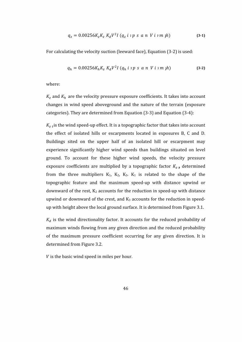
46

= 0.00256 ( ℎ) (3-1)

For calculating the velocity suction (leeward face), Equation (3-2) is used:

= 0.00256 ( ℎ) (3-2)

where:

and are the velocity pressure exposure coefficients. It takes into account

changes in wind speed aboveground and the nature of the terrain (exposure

categories). They are determined from Equation (3-3) and Equation (3-4):

is the wind speed-up effect. It is a topographic factor that takes into account

the effect of isolated hills or escarpments located in exposures B, C and D.

Buildings sited on the upper half of an isolated hill or escarpment may

experience significantly higher wind speeds than buildings situated on level

ground. To account for these higher wind speeds, the velocity pressure

exposure coefficients are multiplied by a topographic factor , determined

from the three multipliers K1, K2, K3. K1 is related to the shape of the

topographic feature and the maximum speed-up with distance upwind or

downward of the rest, K2 accounts for the reduction in speed-up with distance

upwind or downward of the crest, and K3 accounts for the reduction in speed-

up with height above the local ground surface. It is determined from Figure 3.1.

is the wind directionality factor. It accounts for the reduced probability of

maximum winds flowing from any given direction and the reduced probability

of the maximum pressure coefficient occurring for any given direction. It is

determined from Figure 3.2.

is the basic wind speed in miles per hour.

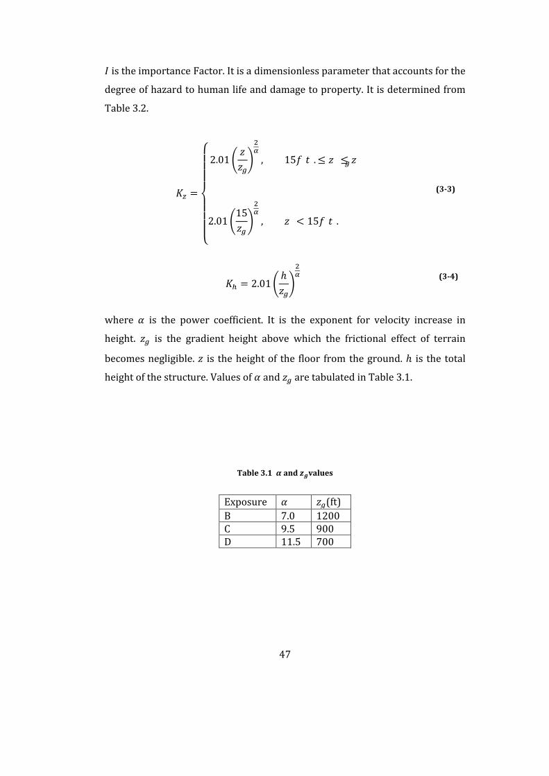
47

is the importance Factor. It is a dimensionless parameter that accounts for the

degree of hazard to human life and damage to property. It is determined from

Table 3.2.

=

⎩⎪⎪⎪⎨⎪⎪⎪⎧ 2.01 , 15 . ≤ ≤

2.01 15 , < 15 .� (3-3)

= 2.01 ℎ (3-4)

where is the power coefficient. It is the exponent for velocity increase in

height. is the gradient height above which the frictional effect of terrain

becomes negligible. is the height of the floor from the ground. ℎ is the total

height of the structure. Values of and are tabulated in Table 3.1.

Table 3.1 and values

Exposure (ft)B 7.0 1200C 9.5 900D 11.5 700

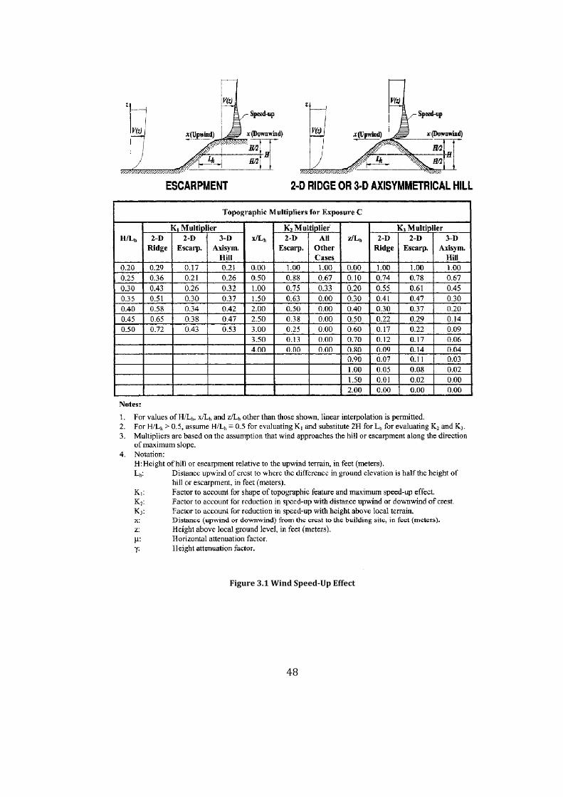
48

Figure 3.1 Wind Speed-Up Effect

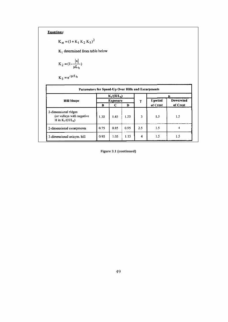
49

Figure 3.1 (continued)

50

Figure 3.2 Wind Directionality Factor

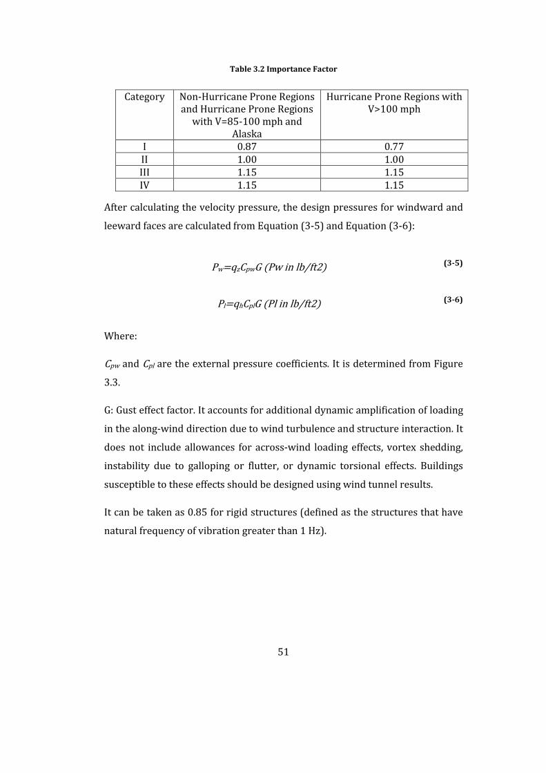
51

Table 3.2 Importance Factor

Category Non-Hurricane Prone Regions and Hurricane Prone Regions

with V=85-100 mph and Alaska

Hurricane Prone Regions with V>100 mph

I 0.87 0.77II 1.00 1.00III 1.15 1.15IV 1.15 1.15

After calculating the velocity pressure, the design pressures for windward and

leeward faces are calculated from Equation (3-5) and Equation (3-6):

Pw=qzCpwG (Pw in lb/ft2) (3-5)

Pl=qhCplG (Pl in lb/ft2) (3-6)

Where:

Cpw and Cpl are the external pressure coefficients. It is determined from Figure

3.3.

G: Gust effect factor. It accounts for additional dynamic amplification of loading

in the along-wind direction due to wind turbulence and structure interaction. It

does not include allowances for across-wind loading effects, vortex shedding,

instability due to galloping or flutter, or dynamic torsional effects. Buildings

susceptible to these effects should be designed using wind tunnel results.

It can be taken as 0.85 for rigid structures (defined as the structures that have

natural frequency of vibration greater than 1 Hz).

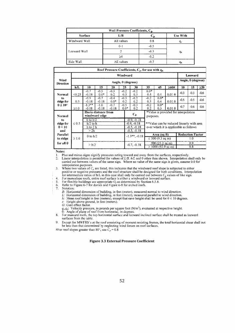
52

Figure 3.3 External Pressure Coefficient

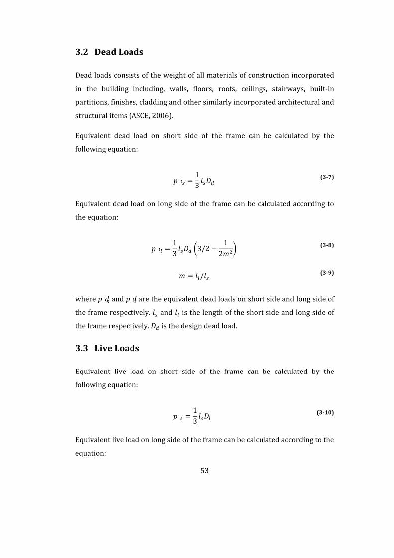
53

3.2 Dead Loads

Dead loads consists of the weight of all materials of construction incorporated

in the building including, walls, floors, roofs, ceilings, stairways, built-in

partitions, finishes, cladding and other similarly incorporated architectural and

structural items (ASCE, 2006).

Equivalent dead load on short side of the frame can be calculated by the

following equation:

= 13 (3-7)

Equivalent dead load on long side of the frame can be calculated according to

the equation:

= 13 3/2 − 12 (3-8)

= / (3-9)

where and are the equivalent dead loads on short side and long side of

the frame respectively. and is the length of the short side and long side of

the frame respectively. is the design dead load.

3.3 Live Loads

Equivalent live load on short side of the frame can be calculated by the

following equation:

= 13 (3-10)

Equivalent live load on long side of the frame can be calculated according to the

equation:

54

= 13 3/2 − 12 (3-11)

= / (3-12)

where and are the equivalent live loads on short side and long side of the

frame respectively. is the design live load.

3.4 Snow Load

Calculation of snow loads are similar to the calculation of dead and live loads:

= 13 (3-13)

= 13 3/2 − 12 (3-14)

= / (3-15)

where and are the equivalent snow loads on short side and long side of

the frame respectively. is the length of the short side of the frame. is the

design snow load.

Numerical values of the deign loads are given in Chapter 6.

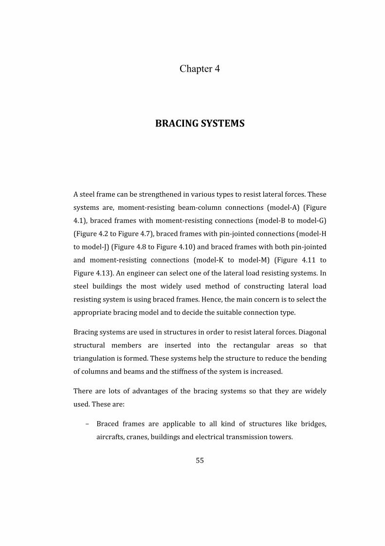
55

Chapter 4

BRACING SYSTEMS

A steel frame can be strengthened in various types to resist lateral forces. These

systems are, moment-resisting beam-column connections (model-A) (Figure

4.1), braced frames with moment-resisting connections (model-B to model-G)

(Figure 4.2 to Figure 4.7), braced frames with pin-jointed connections (model-H

to model-J) (Figure 4.8 to Figure 4.10) and braced frames with both pin-jointed

and moment-resisting connections (model-K to model-M) (Figure 4.11 to

Figure 4.13). An engineer can select one of the lateral load resisting systems. In

steel buildings the most widely used method of constructing lateral load

resisting system is using braced frames. Hence, the main concern is to select the

appropriate bracing model and to decide the suitable connection type.

Bracing systems are used in structures in order to resist lateral forces. Diagonal

structural members are inserted into the rectangular areas so that

triangulation is formed. These systems help the structure to reduce the bending

of columns and beams and the stiffness of the system is increased.

There are lots of advantages of the bracing systems so that they are widely

used. These are:

- Braced frames are applicable to all kind of structures like bridges,

aircrafts, cranes, buildings and electrical transmission towers.

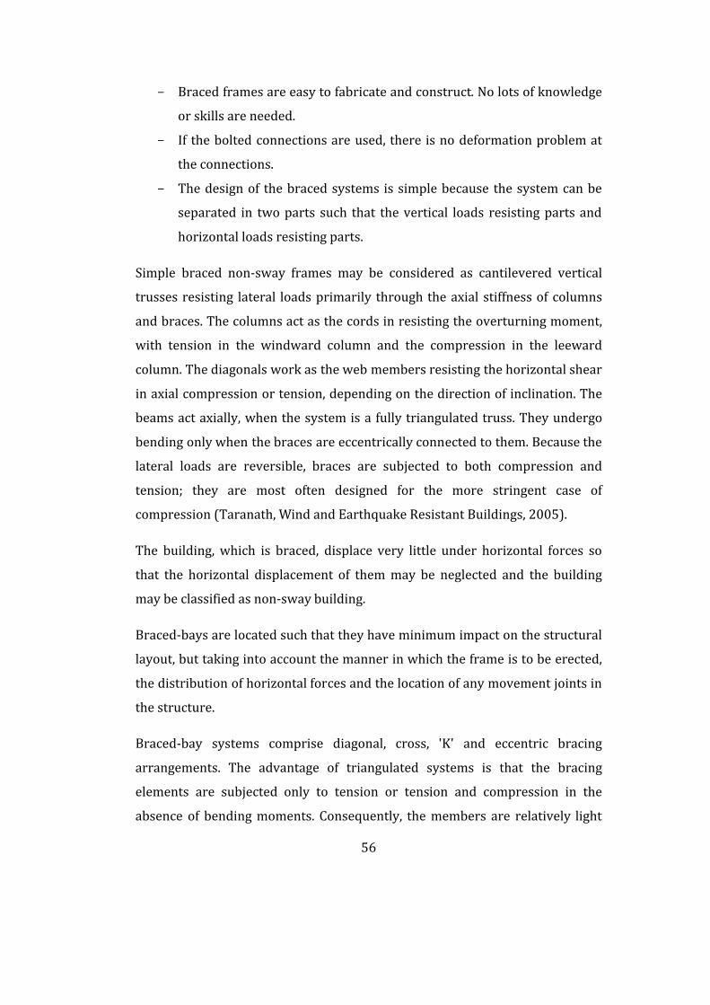
56

- Braced frames are easy to fabricate and construct. No lots of knowledge

or skills are needed.

- If the bolted connections are used, there is no deformation problem at

the connections.

- The design of the braced systems is simple because the system can be

separated in two parts such that the vertical loads resisting parts and

horizontal loads resisting parts.

Simple braced non-sway frames may be considered as cantilevered vertical

trusses resisting lateral loads primarily through the axial stiffness of columns

and braces. The columns act as the cords in resisting the overturning moment,

with tension in the windward column and the compression in the leeward

column. The diagonals work as the web members resisting the horizontal shear

in axial compression or tension, depending on the direction of inclination. The

beams act axially, when the system is a fully triangulated truss. They undergo

bending only when the braces are eccentrically connected to them. Because the

lateral loads are reversible, braces are subjected to both compression and

tension; they are most often designed for the more stringent case of

compression (Taranath, Wind and Earthquake Resistant Buildings, 2005).

The building, which is braced, displace very little under horizontal forces so

that the horizontal displacement of them may be neglected and the building

may be classified as non-sway building.

Braced-bays are located such that they have minimum impact on the structural

layout, but taking into account the manner in which the frame is to be erected,

the distribution of horizontal forces and the location of any movement joints in

the structure.

Braced-bay systems comprise diagonal, cross, 'K' and eccentric bracing

arrangements. The advantage of triangulated systems is that the bracing

elements are subjected only to tension or tension and compression in the

absence of bending moments. Consequently, the members are relatively light

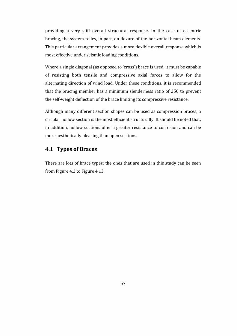
57

providing a very stiff overall structural response. In the case of eccentric

bracing, the system relies, in part, on flexure of the horizontal beam elements.

This particular arrangement provides a more flexible overall response which is

most effective under seismic loading conditions.

Where a single diagonal (as opposed to 'cross') brace is used, it must be capable

of resisting both tensile and compressive axial forces to allow for the

alternating direction of wind load. Under these conditions, it is recommended

that the bracing member has a minimum slenderness ratio of 250 to prevent

the self-weight deflection of the brace limiting its compressive resistance.

Although many different section shapes can be used as compression braces, a

circular hollow section is the most efficient structurally. It should be noted that,

in addition, hollow sections offer a greater resistance to corrosion and can be

more aesthetically pleasing than open sections.

4.1 Types of Braces

There are lots of brace types; the ones that are used in this study can be seen

from Figure 4.2 to Figure 4.13.

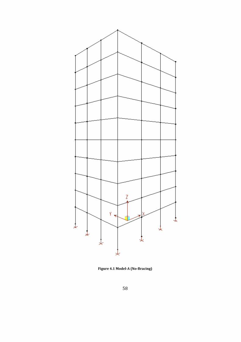
58

Figure 4.1 Model-A (No-Bracing)

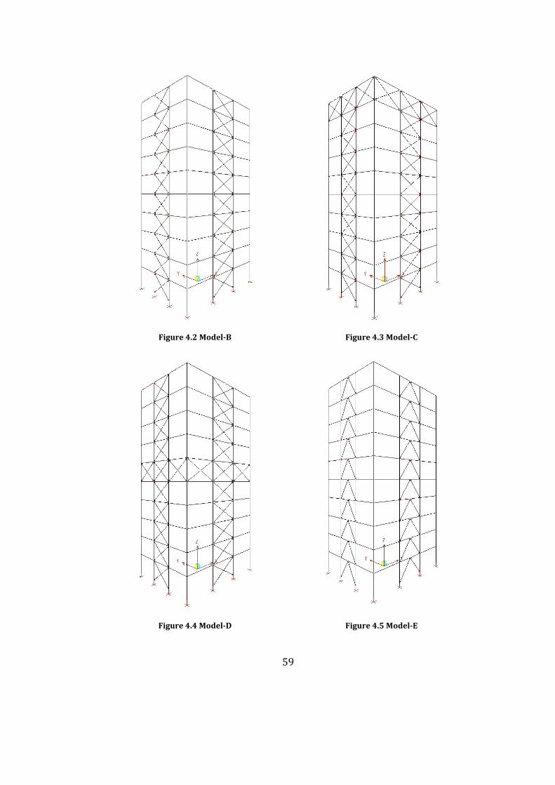
59

Figure 4.2 Model-B Figure 4.3 Model-C

Figure 4.4 Model-D Figure 4.5 Model-E

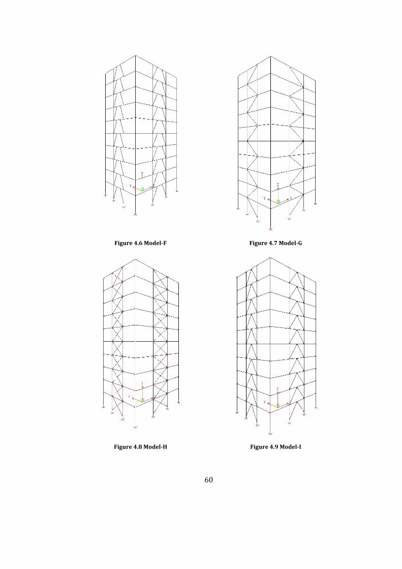
60

Figure 4.6 Model-F Figure 4.7 Model-G

Figure 4.8 Model-H Figure 4.9 Model-I

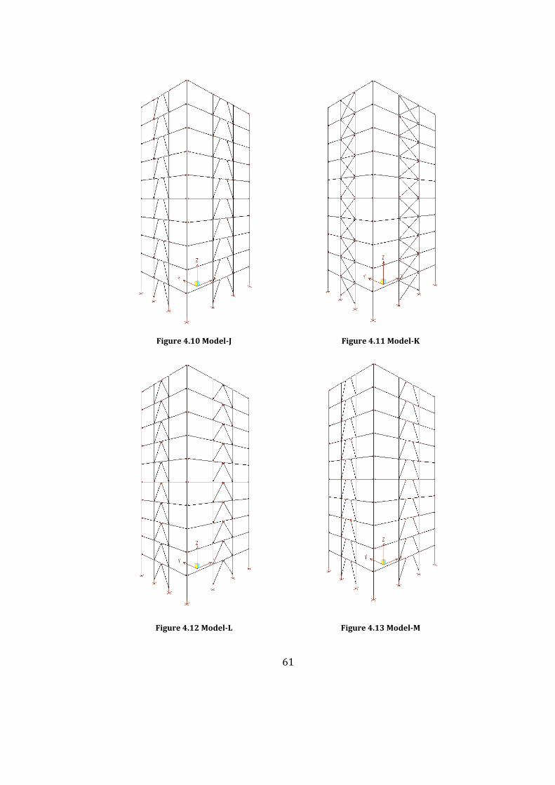
61

Figure 4.10 Model-J Figure 4.11 Model-K

Figure 4.12 Model-L Figure 4.13 Model-M

62

- Model A: No bracing, all column and beam connections are rigid.

- Model B: Middle span is supported by X-type framework and all beam

and column connections are rigid.

- Model C: Middle span is supported by X-type framework and all beam

and column connections are rigid. Moreover top floor is supported by X-

type framework.

- Model D: Middle span is supported by X-type framework and all beam

and column connections are rigid. Moreover middle floor is supported

by X-type framework.

- Model E: Middle span is supported by K-type framework and all beam

and column connections are rigid.

- Model F: Middle span is supported by Knee-type framework and all

beam and column connections are rigid.

- Model G: Middle span is supported by Z-type framework and all beam

and column connections are rigid.

- Model H: Middle span is supported by X-type framework and all beam

and column connections are pin-jointed.

- Model I: Middle span is supported by K-type framework and all beam

and column connections are pin-jointed.

- Model J: Middle span is supported by Knee-type framework and all

beam and column connections are pin-jointed.

- Model K: Middle span is supported by X-type framework and only outer

most beam-column connections are joints.

- Model L: Middle span is supported by K-type framework and only outer

most beam-column connections are pin-jointed.

- Model M: Middle span is supported by Knee-type framework and only

outer most beam-column connections are pin-jointed.,

63

Chapter 5

COST ANALYSIS OF STRUCTURES

Realistic structural design optimization should consider real structural

properties, multiple load cases, and constraints representing all ultimate and

serviceability limit state design rules. In many studies, structure having the

least design weight is considered to be the most economic one. However, this is

only an assumption that the minimal weight could lead to reasonable low

overall costs.

Structural costs of the models in present study are found according to the

formulas given in Pavlovic, Krajnc, & Beg (2004).

Cost of a structure is mainly composed of five elements. These are total

material cost of the elements ( ), total material and manufacturing cost of

joints ( ), total transportation costs ( ), total erection costs ( ) and extra

costs ( ). Cost of the structure (C ) can be formulated as:

= + + + + (5-1)

64

5.1 Cost of the Elements

Steel costs for the elements depend on the mass of all structural elements and

total cost of elements ( ) can be calculated as:

= (5-2)

where = 0.40 is the unit price of steel in /, is the mass of all

elements in the structure in .

5.2 Cost of the Joints

The assessment of the costs for joints is more complex and contains the sum of

different process costs. The cost of joints ( ) can be calculated as:

= + (5-3)

= + + + (5-4)

= + ℎ (5-5)

Where:

- is the total material cost of joints in , is the total

manufacturing cost of joints in .

- , , , are cost of welding material, cost of bolting material,

cost of stiffener material and cost of end plate material respectively.

- is the total manufacturing cost of welding in and is the

total manufacturing cost of hole forming in .

65

5.2.1 Material Cost of Joints

= + + + (5-6)

= (5-7)

= (5-8)

= (5-9)

= (5-10)

where:

- = 1.40 is the unit price of welding material in /, = 1.33 + 0.19 − 0.02 is the material consumption for welding

in / , is the total length of welding in . is the welding size

in and during this study it is taken equal to the plate thickness.

- = 3.076 − 7.373 + 4.62is the unit price of bolt in / ,

is the total number of bolts and is the bolt diameter in .

- = 0.40 is the unit price of steel in /, is the total mass of

stiffener material in .

- is the total mass of plate material in .- The cost for the middle connection of the x-type bracing members with

each other is neglected for all models comprising x-type bracing.

66

5.2.2 Manufacturing Cost of Joints

= + ℎ (5-11)

= ( + ) (5-12)

ℎ = ( ( + )/ + ) (5-13)

where:

- = 0.123 is the unit price of welding manufacturing in / .

= 1.40 is a factor that increases labor. is the operation time

per unit length of weld in / and it is calculated from

(17.26 + 2.9 + 1.82), where a is the weld size in . is the

welding length in . = 0.3 is the any additional welding time in

.

- = 0.323 is the unit price of hole forming in / .is the

number of holes. is the thickness of drilled plate in . is the

additional drilling path in . is the drilling speed in / and

it is calculated from (0.763 − 5.720 + 20.96), where is the hole

diameter in . = 11.9 is the additional time for preparation etc

in .

5.3 Cost of Transportation

Since it is a difficult task to identify the transportation costs, cost estimation of

transportation refers to the total mass of elements. We have to be aware that it

is only an approximation. Therefore cost of transportation ( ) can be

calculated as:

67

= (5-14)

Where = 0.022 is the unit price of transportation in / .is the total

mass of the structure in .

5.4 Cost of Erection

Similar to the cost of transportation, cost of erection is a function of the mass of

the structure. Cost of erection ( ) can be calculated as:

= (5-15)

where = 120.20 is the unit price of man-hour considering the man and

machine power and it is in /ℎ. = 0.0014 is the man-hour per unit

quantity of the steel in ℎ / .5.5 Extra Costs

In a building there are lots of extra costs that have to be taken into account.

These are painting, flange aligning, surface preparation, cutting and welding of

the elements. Since the models that are studied are very similar, for simplicity,

the other costs are taken as a function of the mass of the structure. Extra costs

are taken equal to 0.184 / for all of the models. This value is decided

according to the sample problem solved in Pavlovic, Krajnc, & Beg, (2004).

68

Chapter 6

TEST STRUCTURES

Three different structures with 10, 20 and 30 stories are considered and for

every structure all of the prescribed bracing models are applied. Therefore 39

different models with practical design considerations are studied to compare

performances of different bracing models and frame types. They are designed

for minimum weight considering cross-sections of the members being the

design variables. The costs of the models are calculated after the designs are

completed regarding the minimum weight. For all design examples, the

following material properties of the steel are used: modulus of elasticity (E) =

29,000 ksi (203,893.6 MPa) and yield stress ( yF ) = 36 ksi (253.1 MPa).

It is necessary to prepare a design pool, where a set of steel sections selected

from available profile lists in the design code are collected and sorted in

descending order. The sequence numbers assigned to these sections vary

between 1 to total number of sections included in the design pool. This

sequence number is treated as design variable. For example, if there are 272

steel sections in the design pool and 35 member groups in the frame to be

designed then the ES technique selects randomly an integer number which has

a value between 1 and 272 for each member group. Once this selection is

carried out for each group, the cross sectional properties of each steel section

become available from the design pool. The structure is then analyzed under

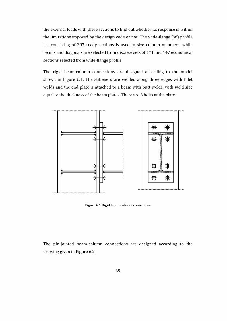
69

the external loads with these sections to find out whether its response is within

the limitations imposed by the design code or not. The wide-flange (W) profile

list consisting of 297 ready sections is used to size column members, while

beams and diagonals are selected from discrete sets of 171 and 147 economical

sections selected from wide-flange profile.

The rigid beam-column connections are designed according to the model

shown in Figure 6.1. The stiffeners are welded along three edges with fillet

welds and the end plate is attached to a beam with butt welds, with weld size

equal to the thickness of the beam plates. There are 8 bolts at the plate.

Figure 6.1 Rigid beam-column connection

The pin-jointed beam-column connections are designed according to the

drawing given in Figure 6.2.

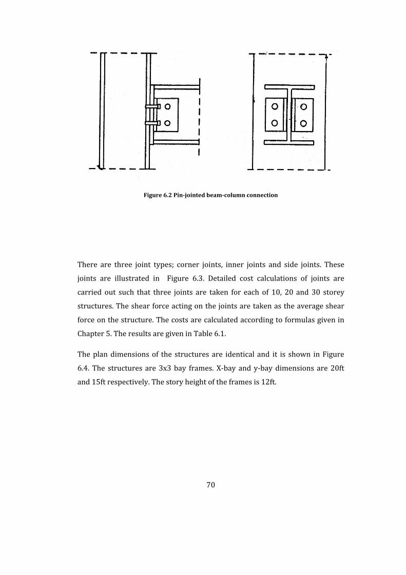
70

Figure 6.2 Pin-jointed beam-column connection

There are three joint types; corner joints, inner joints and side joints. These

joints are illustrated in Figure 6.3. Detailed cost calculations of joints are

carried out such that three joints are taken for each of 10, 20 and 30 storey

structures. The shear force acting on the joints are taken as the average shear

force on the structure. The costs are calculated according to formulas given in

Chapter 5. The results are given in Table 6.1.

The plan dimensions of the structures are identical and it is shown in Figure

6.4. The structures are 3x3 bay frames. X-bay and y-bay dimensions are 20ft

and 15ft respectively. The story height of the frames is 12ft.

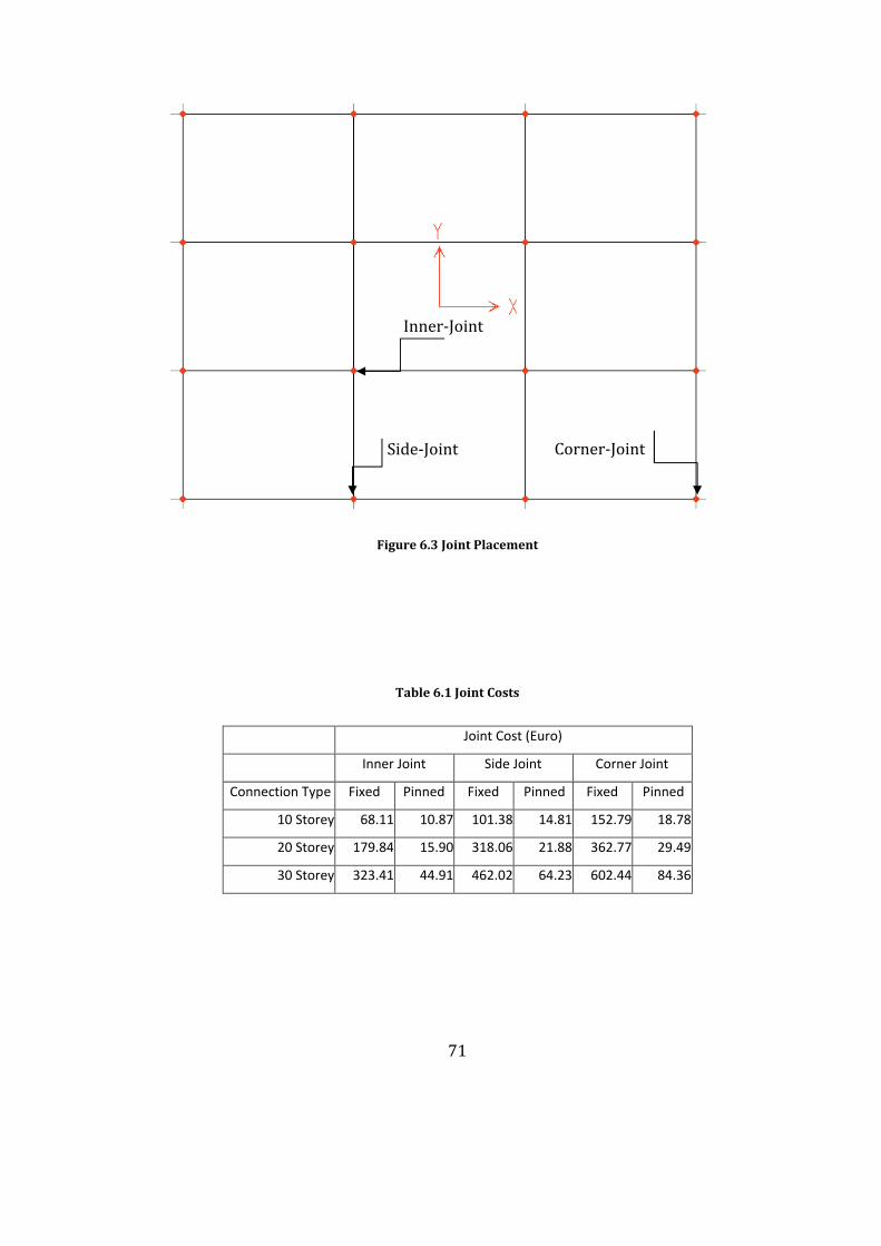
71

Figure 6.3 Joint Placement

Table 6.1 Joint Costs

Joint Cost (Euro)

Inner Joint Side Joint Corner Joint

Connection Type Fixed Pinned Fixed Pinned Fixed Pinned

10 Storey 68.11 10.87 101.38 14.81 152.79 18.78

20 Storey 179.84 15.90 318.06 21.88 362.77 29.49

30 Storey 323.41 44.91 462.02 64.23 602.44 84.36

Side-Joint Corner-Joint

Inner-Joint

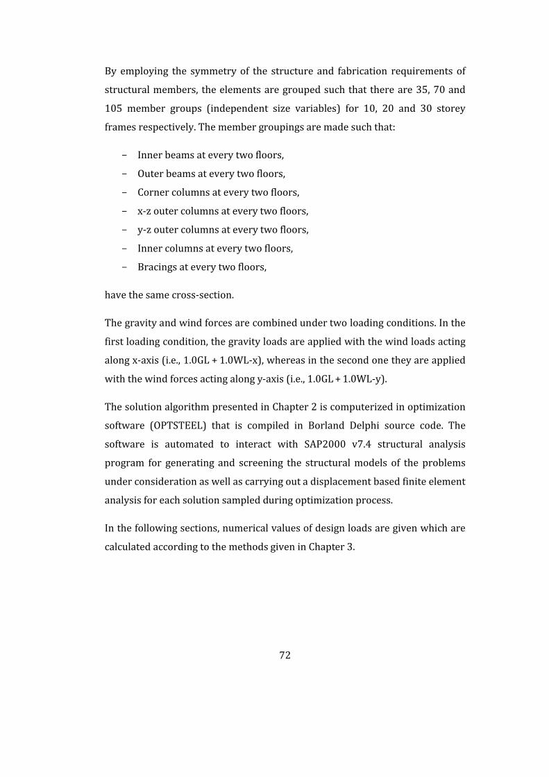
72

By employing the symmetry of the structure and fabrication requirements of

structural members, the elements are grouped such that there are 35, 70 and

105 member groups (independent size variables) for 10, 20 and 30 storey

frames respectively. The member groupings are made such that:

- Inner beams at every two floors,

- Outer beams at every two floors,

- Corner columns at every two floors,

- x-z outer columns at every two floors,

- y-z outer columns at every two floors,

- Inner columns at every two floors,

- Bracings at every two floors,

have the same cross-section.

The gravity and wind forces are combined under two loading conditions. In the

first loading condition, the gravity loads are applied with the wind loads acting

along x-axis (i.e., 1.0GL + 1.0WL-x), whereas in the second one they are applied

with the wind forces acting along y-axis (i.e., 1.0GL + 1.0WL-y).

The solution algorithm presented in Chapter 2 is computerized in optimization

software (OPTSTEEL) that is compiled in Borland Delphi source code. The

software is automated to interact with SAP2000 v7.4 structural analysis

program for generating and screening the structural models of the problems

under consideration as well as carrying out a displacement based finite element

analysis for each solution sampled during optimization process.

In the following sections, numerical values of design loads are given which are

calculated according to the methods given in Chapter 3.

73

Figure 6.4 Typical plan view of the models

20 ft.

15 ft.

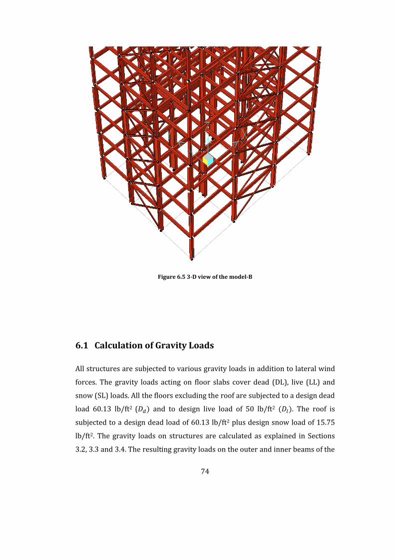
74

Figure 6.5 3-D view of the model-B

6.1 Calculation of Gravity Loads

All structures are subjected to various gravity loads in addition to lateral wind

forces. The gravity loads acting on floor slabs cover dead (DL), live (LL) and

snow (SL) loads. All the floors excluding the roof are subjected to a design dead

load 60.13 lb/ft2 ( ) and to design live load of 50 lb/ft2 ( ). The roof is

subjected to a design dead load of 60.13 lb/ft2 plus design snow load of 15.75

lb/ft2. The gravity loads on structures are calculated as explained in Sections

3.2, 3.3 and 3.4. The resulting gravity loads on the outer and inner beams of the

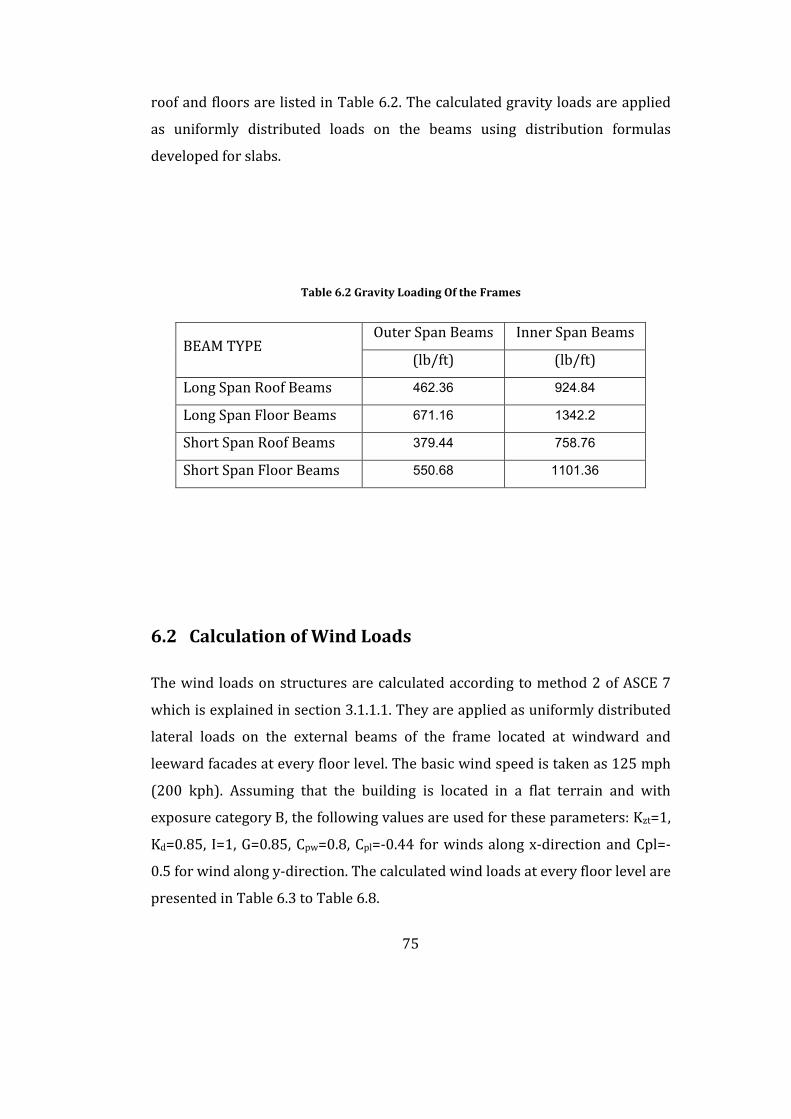
75

roof and floors are listed in Table 6.2. The calculated gravity loads are applied

as uniformly distributed loads on the beams using distribution formulas

developed for slabs.

Table 6.2 Gravity Loading Of the Frames

BEAM TYPEOuter Span Beams Inner Span Beams

(lb/ft) (lb/ft)

Long Span Roof Beams 462.36 924.84

Long Span Floor Beams 671.16 1342.2

Short Span Roof Beams 379.44 758.76

Short Span Floor Beams 550.68 1101.36

6.2 Calculation of Wind Loads

The wind loads on structures are calculated according to method 2 of ASCE 7

which is explained in section 3.1.1.1. They are applied as uniformly distributed

lateral loads on the external beams of the frame located at windward and

leeward facades at every floor level. The basic wind speed is taken as 125 mph

(200 kph). Assuming that the building is located in a flat terrain and with

exposure category B, the following values are used for these parameters: Kzt=1,

Kd=0.85, I=1, G=0.85, Cpw=0.8, Cpl=-0.44 for winds along x-direction and Cpl=-

0.5 for wind along y-direction. The calculated wind loads at every floor level are

presented in Table 6.3 to Table 6.8.

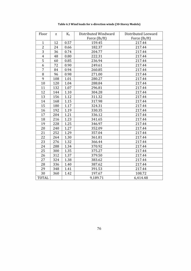
76

Table 6.3 Wind loads for x-direction winds (30-Storey Models)

Floor z Kz Distributed Windward Force (lb/ft)

Distributed Leeward Force (lb/ft)

1 12 0.57 159.45 217.442 24 0.66 182.37 217.443 36 0.74 204.77 217.444 48 0.80 222.31 217.445 60 0.85 236.94 217.446 72 0.90 249.61 217.447 84 0.94 260.85 217.448 96 0.98 271.00 217.449 108 1.01 280.27 217.44

10 120 1.04 288.84 217.4411 132 1.07 296.81 217.4412 144 1.10 304.28 217.4413 156 1.12 311.32 217.4414 168 1.15 317.98 217.4415 180 1.17 324.31 217.4416 192 1.19 330.35 217.4417 204 1.21 336.12 217.4418 216 1.23 341.65 217.4419 228 1.25 346.97 217.4420 240 1.27 352.09 217.4421 252 1.29 357.04 217.4422 264 1.30 361.81 217.4423 276 1.32 366.44 217.4424 288 1.34 370.92 217.4425 300 1.35 375.27 217.4426 312 1.37 379.50 217.4427 324 1.38 383.62 217.4428 336 1.40 387.62 217.4429 348 1.41 391.53 217.4430 360 1.42 197.67 108.72

TOTAL 9,189.71 6,414.48

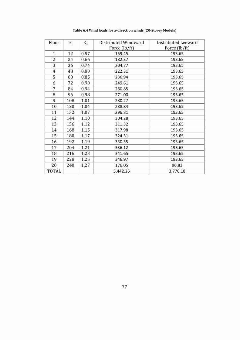
77

Table 6.4 Wind loads for x-direction winds (20-Storey Models)

Floor z Kz Distributed Windward Force (lb/ft)

Distributed Leeward Force (lb/ft)

1 12 0.57 159.45 193.652 24 0.66 182.37 193.653 36 0.74 204.77 193.654 48 0.80 222.31 193.655 60 0.85 236.94 193.656 72 0.90 249.61 193.657 84 0.94 260.85 193.658 96 0.98 271.00 193.659 108 1.01 280.27 193.65

10 120 1.04 288.84 193.6511 132 1.07 296.81 193.6512 144 1.10 304.28 193.6513 156 1.12 311.32 193.6514 168 1.15 317.98 193.6515 180 1.17 324.31 193.6516 192 1.19 330.35 193.6517 204 1.21 336.12 193.6518 216 1.23 341.65 193.6519 228 1.25 346.97 193.6520 240 1.27 176.05 96.83

TOTAL 5,442.25 3,776.18

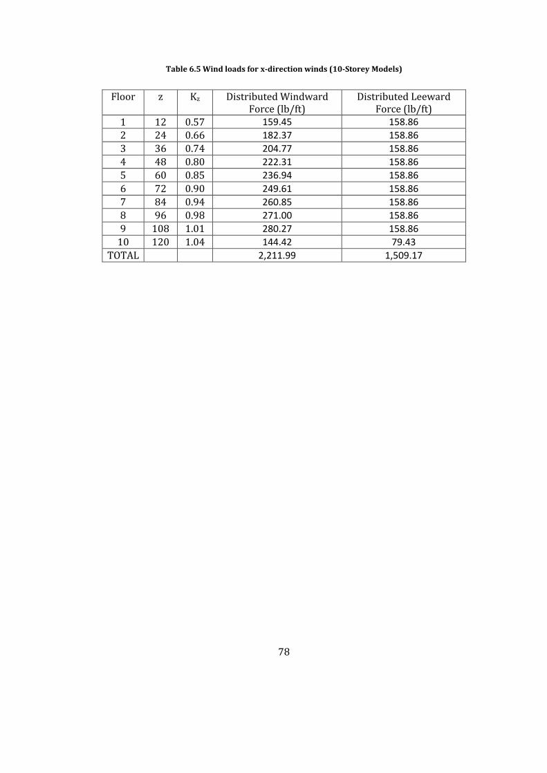
78

Table 6.5 Wind loads for x-direction winds (10-Storey Models)

Floor z Kz Distributed Windward Force (lb/ft)

Distributed Leeward Force (lb/ft)

1 12 0.57 159.45 158.862 24 0.66 182.37 158.863 36 0.74 204.77 158.864 48 0.80 222.31 158.865 60 0.85 236.94 158.866 72 0.90 249.61 158.867 84 0.94 260.85 158.868 96 0.98 271.00 158.869 108 1.01 280.27 158.86

10 120 1.04 144.42 79.43TOTAL 2,211.99 1,509.17

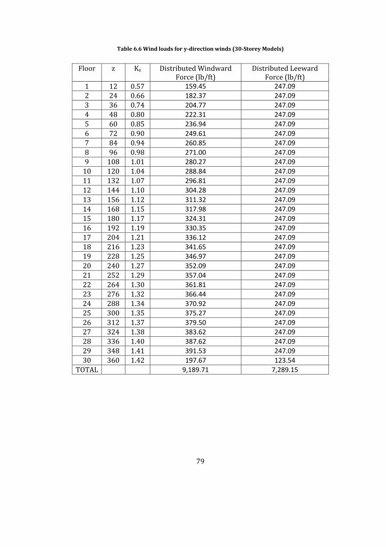
79

Table 6.6 Wind loads for y-direction winds (30-Storey Models)

Floor z Kz Distributed Windward Force (lb/ft)

Distributed Leeward Force (lb/ft)

1 12 0.57 159.45 247.092 24 0.66 182.37 247.093 36 0.74 204.77 247.094 48 0.80 222.31 247.095 60 0.85 236.94 247.096 72 0.90 249.61 247.097 84 0.94 260.85 247.098 96 0.98 271.00 247.099 108 1.01 280.27 247.09

10 120 1.04 288.84 247.0911 132 1.07 296.81 247.0912 144 1.10 304.28 247.0913 156 1.12 311.32 247.0914 168 1.15 317.98 247.0915 180 1.17 324.31 247.0916 192 1.19 330.35 247.0917 204 1.21 336.12 247.0918 216 1.23 341.65 247.0919 228 1.25 346.97 247.0920 240 1.27 352.09 247.0921 252 1.29 357.04 247.0922 264 1.30 361.81 247.0923 276 1.32 366.44 247.0924 288 1.34 370.92 247.0925 300 1.35 375.27 247.0926 312 1.37 379.50 247.0927 324 1.38 383.62 247.0928 336 1.40 387.62 247.0929 348 1.41 391.53 247.0930 360 1.42 197.67 123.54

TOTAL 9,189.71 7,289.15

80

Table 6.7 Wind loads for y-direction winds (20-Storey Models)

Floor z Kz Distributed Windward Force (lb/ft)

Distributed Leeward Force (lb/ft)

1 12 0.57 159.45 220.062 24 0.66 182.37 220.063 36 0.74 204.77 220.064 48 0.80 222.31 220.065 60 0.85 236.94 220.066 72 0.90 249.61 220.067 84 0.94 260.85 220.068 96 0.98 271.00 220.069 108 1.01 280.27 220.06

10 120 1.04 288.84 220.0611 132 1.07 296.81 220.0612 144 1.10 304.28 220.0613 156 1.12 311.32 220.0614 168 1.15 317.98 220.0615 180 1.17 324.31 220.0616 192 1.19 330.35 220.0617 204 1.21 336.12 220.0618 216 1.23 341.65 220.0619 228 1.25 346.97 220.0620 240 1.27 176.05 110.03

TOTAL 5,442.25 4,291.17

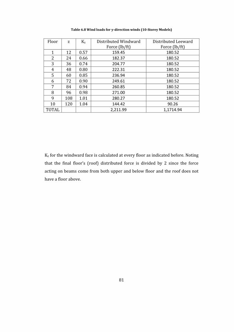
81

Table 6.8 Wind loads for y-direction winds (10-Storey Models)

Floor z Kz Distributed Windward Force (lb/ft)

Distributed Leeward Force (lb/ft)

1 12 0.57 159.45 180.522 24 0.66 182.37 180.523 36 0.74 204.77 180.524 48 0.80 222.31 180.525 60 0.85 236.94 180.526 72 0.90 249.61 180.527 84 0.94 260.85 180.528 96 0.98 271.00 180.529 108 1.01 280.27 180.52

10 120 1.04 144.42 90.26TOTAL 2,211.99 1,1714.94

Kz for the windward face is calculated at every floor as indicated before. Noting

that the final floor’s (roof) distributed force is divided by 2 since the force

acting on beams come from both upper and below floor and the roof does not

have a floor above.

82

Chapter 7

RESULTS AND THEIR INTERPRATATION

7.1 Results

During the study, the optimal configuration of lateral bracing systems in steel

structures to resist wind forces is seeked. For this job three different structures

(10, 20 and 30 stories) with twelve different bracing models are considered.

The optimum designs of all three structures with all bracing models are made.

Due to stochastic nature of these techniques, each design example is

independently solved five times and average performances are considered.

The tabulated results of the steel section for every group number of these three

models can be seen Table 7.1 to Table 7.6. Optimum weights of the models are

found by using OPTSTEEL and these weights are given in Table 7.7. The models

having the minimum weight are model-G, model-E and model-D for 10, 20 and

30 stories respectively.

For each model cost calculations are carried out. This process is handled with

formulas described in Chapter 5. As a result of the calculations the models

leading to minimum costs are model-L for both 10 and 20 stories, model-D for

the 30 floored structures. Costs of all models are presented in Table 7.8, Table

7.9 and Table 7.10.

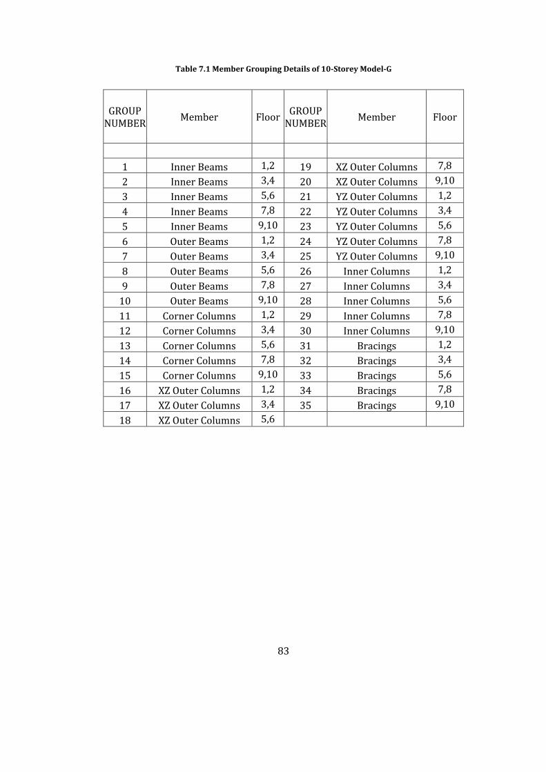
83

Table 7.1 Member Grouping Details of 10-Storey Model-G

GROUP NUMBER

Member Floor GROUP NUMBER

Member Floor

1 Inner Beams 1,2 19 XZ Outer Columns 7,8

2 Inner Beams 3,4 20 XZ Outer Columns 9,10

3 Inner Beams 5,6 21 YZ Outer Columns 1,2

4 Inner Beams 7,8 22 YZ Outer Columns 3,4

5 Inner Beams 9,10 23 YZ Outer Columns 5,6

6 Outer Beams 1,2 24 YZ Outer Columns 7,8

7 Outer Beams 3,4 25 YZ Outer Columns 9,10

8 Outer Beams 5,6 26 Inner Columns 1,2

9 Outer Beams 7,8 27 Inner Columns 3,4

10 Outer Beams 9,10 28 Inner Columns 5,6

11 Corner Columns 1,2 29 Inner Columns 7,8

12 Corner Columns 3,4 30 Inner Columns 9,10

13 Corner Columns 5,6 31 Bracings 1,2

14 Corner Columns 7,8 32 Bracings 3,4

15 Corner Columns 9,10 33 Bracings 5,6

16 XZ Outer Columns 1,2 34 Bracings 7,8

17 XZ Outer Columns 3,4 35 Bracings 9,10

18 XZ Outer Columns 5,6

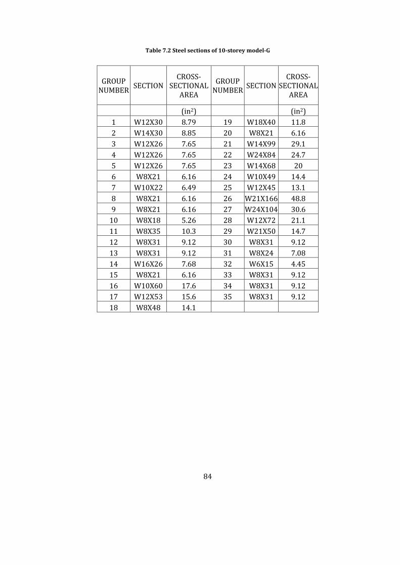
84

Table 7.2 Steel sections of 10-storey model-G

GROUP NUMBER

SECTIONCROSS-

SECTIONAL AREA

GROUP NUMBER

SECTIONCROSS-

SECTIONAL AREA

(in2) (in2)1 W12X30 8.79 19 W18X40 11.82 W14X30 8.85 20 W8X21 6.163 W12X26 7.65 21 W14X99 29.14 W12X26 7.65 22 W24X84 24.75 W12X26 7.65 23 W14X68 206 W8X21 6.16 24 W10X49 14.47 W10X22 6.49 25 W12X45 13.18 W8X21 6.16 26 W21X166 48.89 W8X21 6.16 27 W24X104 30.6

10 W8X18 5.26 28 W12X72 21.111 W8X35 10.3 29 W21X50 14.712 W8X31 9.12 30 W8X31 9.1213 W8X31 9.12 31 W8X24 7.0814 W16X26 7.68 32 W6X15 4.4515 W8X21 6.16 33 W8X31 9.1216 W10X60 17.6 34 W8X31 9.1217 W12X53 15.6 35 W8X31 9.1218 W8X48 14.1

85

Table 7.3 Member Grouping Details of 20-Storey Model-E

Table 7.3 (Continued)

GROUP NUMBER MEMBER FLOOR

GROUP NUMBER MEMBER FLOOR

1 Inner Beams 1,2 36 XZ Outer Columns 11,12

2 Inner Beams 3,4 37 XZ Outer Columns 13,14

3 Inner Beams 5,6 38 XZ Outer Columns 15,16

4 Inner Beams 7,8 39 XZ Outer Columns 17,18

5 Inner Beams 9,10 40 XZ Outer Columns 19,20

6 Inner Beams 11,12 41 YZ Outer Columns 1,2

7 Inner Beams 13,14 42 YZ Outer Columns 3,4

8 Inner Beams 15,16 43 YZ Outer Columns 5,6

9 Inner Beams 17,18 44 YZ Outer Columns 7,8

10 Inner Beams 19,20 45 YZ Outer Columns 9,10

11 Outer Beams 1,2 46 YZ Outer Columns 11,12

12 Outer Beams 3,4 47 YZ Outer Columns 13,14

13 Outer Beams 5,6 48 YZ Outer Columns 15,16

14 Outer Beams 7,8 49 YZ Outer Columns 17,18

15 Outer Beams 9,10 50 YZ Outer Columns 19,20

16 Outer Beams 11,12 51 Inner Columns 1,2

17 Outer Beams 13,14 52 Inner Columns 3,4

18 Outer Beams 15,16 53 Inner Columns 5,6

19 Outer Beams 17,18 54 Inner Columns 7,8

20 Outer Beams 19,20 55 Inner Columns 9,10

21 Corner Columns 1,2 56 Inner Columns 11,12

22 Corner Columns 3,4 57 Inner Columns 13,14

23 Corner Columns 5,6 58 Inner Columns 15,16

24 Corner Columns 7,8 59 Inner Columns 17,18

25 Corner Columns 9,10 60 Inner Columns 19,20

26 Corner Columns 11,12 61 Bracings 1,2

27 Corner Columns 13,14 62 Bracings 3,4

28 Corner Columns 15,16 63 Bracings 5,6

29 Corner Columns 17,18 64 Bracings 7,8

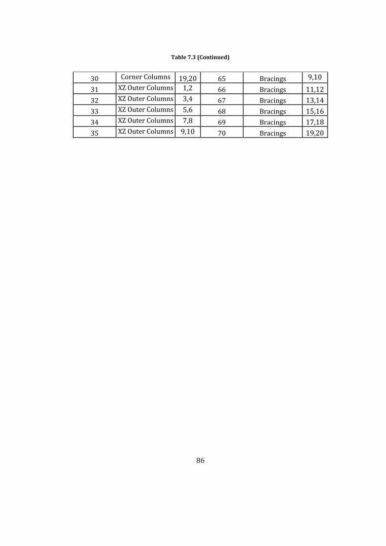
86

Table 7.3 (Continued)

30 Corner Columns 19,20 65 Bracings 9,10

31 XZ Outer Columns 1,2 66 Bracings 11,12

32 XZ Outer Columns 3,4 67 Bracings 13,14

33 XZ Outer Columns 5,6 68 Bracings 15,16

34 XZ Outer Columns 7,8 69 Bracings 17,18

35 XZ Outer Columns 9,10 70 Bracings 19,20

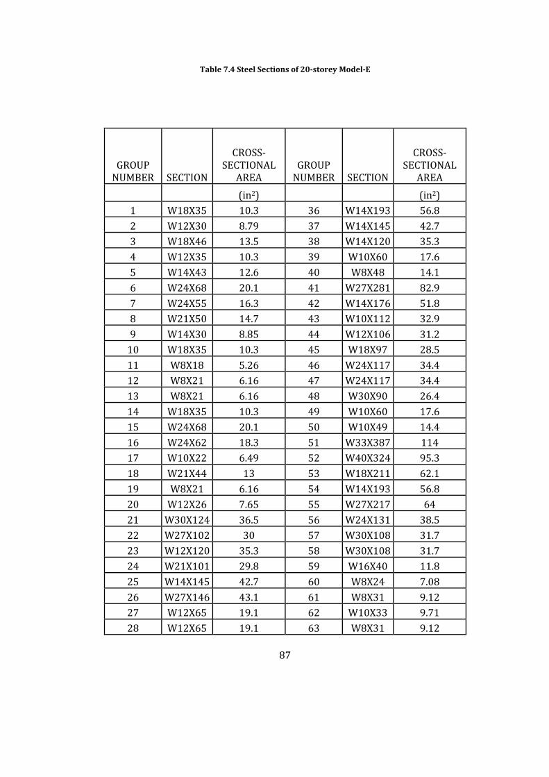
87

Table 7.4 Steel Sections of 20-storey Model-E

Table 7.4 (Continued)

GROUP NUMBER SECTION

CROSS-SECTIONAL

AREAGROUP

NUMBER SECTION

CROSS-SECTIONAL

AREA

(in2) (in2)1 W18X35 10.3 36 W14X193 56.82 W12X30 8.79 37 W14X145 42.73 W18X46 13.5 38 W14X120 35.34 W12X35 10.3 39 W10X60 17.65 W14X43 12.6 40 W8X48 14.16 W24X68 20.1 41 W27X281 82.97 W24X55 16.3 42 W14X176 51.88 W21X50 14.7 43 W10X112 32.99 W14X30 8.85 44 W12X106 31.2

10 W18X35 10.3 45 W18X97 28.511 W8X18 5.26 46 W24X117 34.412 W8X21 6.16 47 W24X117 34.413 W8X21 6.16 48 W30X90 26.414 W18X35 10.3 49 W10X60 17.615 W24X68 20.1 50 W10X49 14.416 W24X62 18.3 51 W33X387 11417 W10X22 6.49 52 W40X324 95.318 W21X44 13 53 W18X211 62.119 W8X21 6.16 54 W14X193 56.820 W12X26 7.65 55 W27X217 6421 W30X124 36.5 56 W24X131 38.522 W27X102 30 57 W30X108 31.723 W12X120 35.3 58 W30X108 31.724 W21X101 29.8 59 W16X40 11.825 W14X145 42.7 60 W8X24 7.0826 W27X146 43.1 61 W8X31 9.1227 W12X65 19.1 62 W10X33 9.7128 W12X65 19.1 63 W8X31 9.12

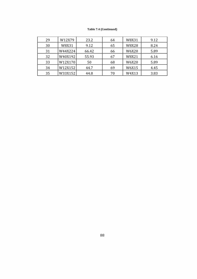
88

Table 7.4 (Continued)

29 W12X79 23.2 64 W8X31 9.1230 W8X31 9.12 65 W8X28 8.2431 W44X224 66.42 66 W6X20 5.8932 W40X192 55.93 67 W8X21 6.1633 W12X170 50 68 W6X20 5.8934 W12X152 44.7 69 W6X15 4.4535 W33X152 44.8 70 W4X13 3.83

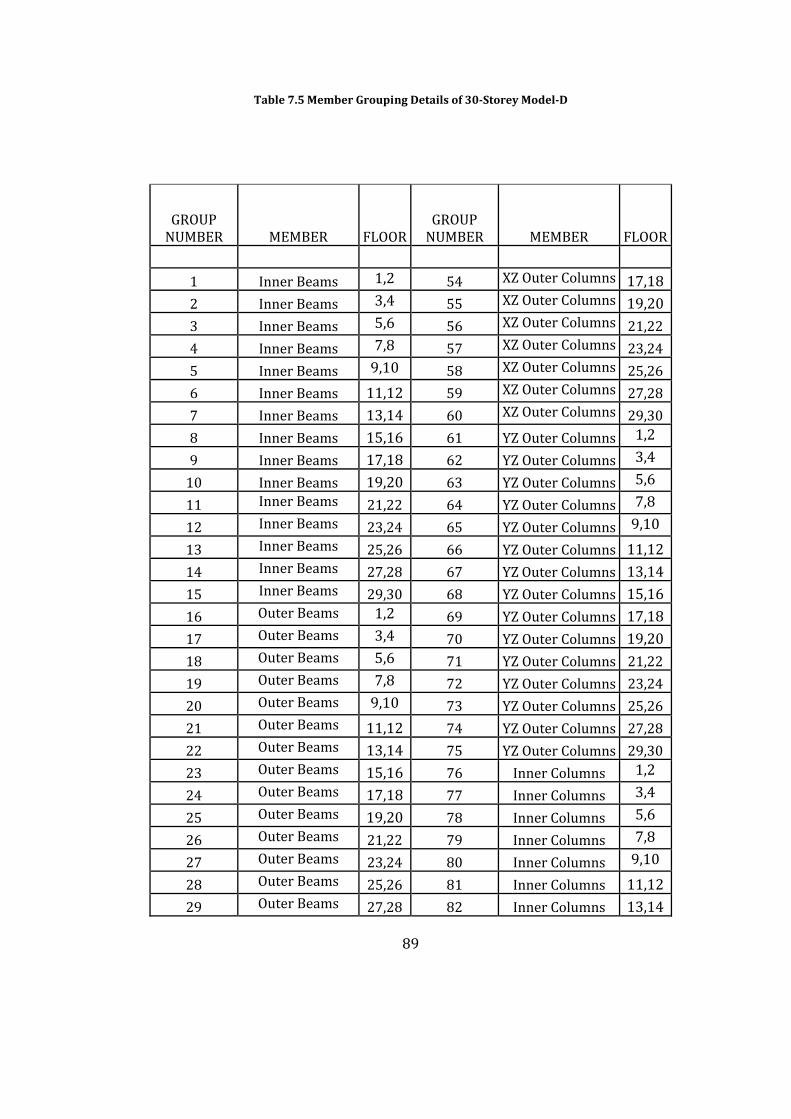
89

Table 7.5 Member Grouping Details of 30-Storey Model-D

Table 7.5 (Continued)

GROUP NUMBER MEMBER FLOOR

GROUP NUMBER MEMBER FLOOR

1 Inner Beams 1,2 54 XZ Outer Columns 17,18

2 Inner Beams 3,4 55 XZ Outer Columns 19,20

3 Inner Beams 5,6 56 XZ Outer Columns 21,22

4 Inner Beams 7,8 57 XZ Outer Columns 23,24

5 Inner Beams 9,10 58 XZ Outer Columns 25,26

6 Inner Beams 11,12 59 XZ Outer Columns 27,28

7 Inner Beams 13,14 60 XZ Outer Columns 29,30

8 Inner Beams 15,16 61 YZ Outer Columns 1,2

9 Inner Beams 17,18 62 YZ Outer Columns 3,4

10 Inner Beams 19,20 63 YZ Outer Columns 5,6

11 Inner Beams 21,22 64 YZ Outer Columns 7,8

12 Inner Beams 23,24 65 YZ Outer Columns 9,10

13 Inner Beams 25,26 66 YZ Outer Columns 11,12

14 Inner Beams 27,28 67 YZ Outer Columns 13,14

15 Inner Beams 29,30 68 YZ Outer Columns 15,16

16 Outer Beams 1,2 69 YZ Outer Columns 17,18

17 Outer Beams 3,4 70 YZ Outer Columns 19,20

18 Outer Beams 5,6 71 YZ Outer Columns 21,22

19 Outer Beams 7,8 72 YZ Outer Columns 23,24

20 Outer Beams 9,10 73 YZ Outer Columns 25,26

21 Outer Beams 11,12 74 YZ Outer Columns 27,28

22 Outer Beams 13,14 75 YZ Outer Columns 29,30

23 Outer Beams 15,16 76 Inner Columns 1,2

24 Outer Beams 17,18 77 Inner Columns 3,4

25 Outer Beams 19,20 78 Inner Columns 5,6

26 Outer Beams 21,22 79 Inner Columns 7,8

27 Outer Beams 23,24 80 Inner Columns 9,10

28 Outer Beams 25,26 81 Inner Columns 11,12

29 Outer Beams 27,28 82 Inner Columns 13,14

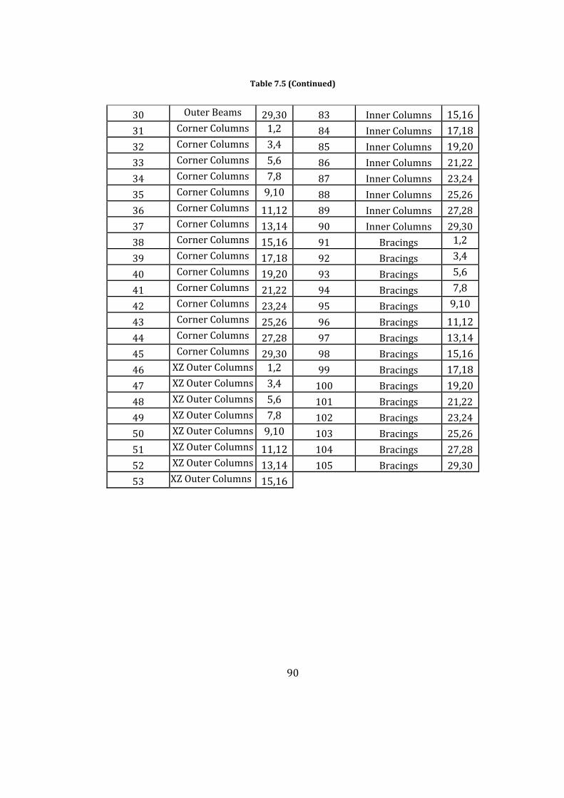
90

Table 7.5 (Continued)

30 Outer Beams 29,30 83 Inner Columns 15,16

31 Corner Columns 1,2 84 Inner Columns 17,18

32 Corner Columns 3,4 85 Inner Columns 19,20

33 Corner Columns 5,6 86 Inner Columns 21,22

34 Corner Columns 7,8 87 Inner Columns 23,24

35 Corner Columns 9,10 88 Inner Columns 25,26

36 Corner Columns 11,12 89 Inner Columns 27,28

37 Corner Columns 13,14 90 Inner Columns 29,30

38 Corner Columns 15,16 91 Bracings 1,2

39 Corner Columns 17,18 92 Bracings 3,4

40 Corner Columns 19,20 93 Bracings 5,6

41 Corner Columns 21,22 94 Bracings 7,8

42 Corner Columns 23,24 95 Bracings 9,10

43 Corner Columns 25,26 96 Bracings 11,12

44 Corner Columns 27,28 97 Bracings 13,14

45 Corner Columns 29,30 98 Bracings 15,16

46 XZ Outer Columns 1,2 99 Bracings 17,18

47 XZ Outer Columns 3,4 100 Bracings 19,20

48 XZ Outer Columns 5,6 101 Bracings 21,22

49 XZ Outer Columns 7,8 102 Bracings 23,24

50 XZ Outer Columns 9,10 103 Bracings 25,26

51 XZ Outer Columns 11,12 104 Bracings 27,28

52 XZ Outer Columns 13,14 105 Bracings 29,30

53 XZ Outer Columns 15,16

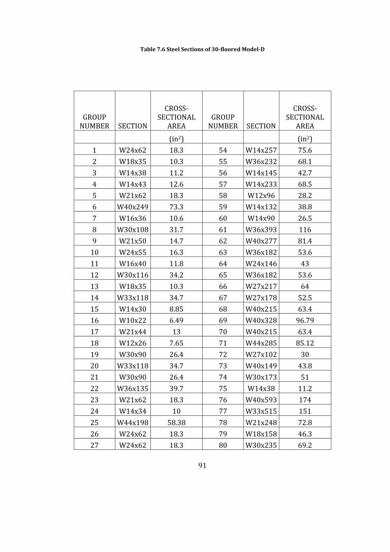
91

Table 7.6 Steel Sections of 30-floored Model-D

Table 7.6 (Continued)

GROUP NUMBER SECTION

CROSS-SECTIONAL

AREAGROUP

NUMBER SECTION

CROSS-SECTIONAL

AREA

(in2) (in2)

1 W24x62 18.3 54 W14x257 75.6

2 W18x35 10.3 55 W36x232 68.1

3 W14x38 11.2 56 W14x145 42.7

4 W14x43 12.6 57 W14x233 68.5

5 W21x62 18.3 58 W12x96 28.2

6 W40x249 73.3 59 W14x132 38.8

7 W16x36 10.6 60 W14x90 26.5

8 W30x108 31.7 61 W36x393 116

9 W21x50 14.7 62 W40x277 81.4

10 W24x55 16.3 63 W36x182 53.6

11 W16x40 11.8 64 W24x146 43

12 W30x116 34.2 65 W36x182 53.6

13 W18x35 10.3 66 W27x217 64

14 W33x118 34.7 67 W27x178 52.5

15 W14x30 8.85 68 W40x215 63.4

16 W10x22 6.49 69 W40x328 96.79

17 W21x44 13 70 W40x215 63.4

18 W12x26 7.65 71 W44x285 85.12

19 W30x90 26.4 72 W27x102 30

20 W33x118 34.7 73 W40x149 43.8

21 W30x90 26.4 74 W30x173 51

22 W36x135 39.7 75 W14x38 11.2

23 W21x62 18.3 76 W40x593 174

24 W14x34 10 77 W33x515 151

25 W44x198 58.38 78 W21x248 72.8

26 W24x62 18.3 79 W18x158 46.3

27 W24x62 18.3 80 W30x235 69.2

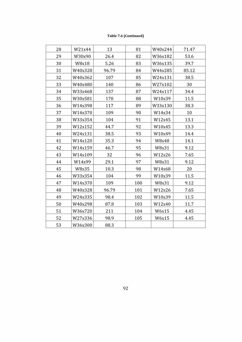
92

Table 7.6 (Continued)

28 W21x44 13 81 W40x244 71.47

29 W30x90 26.4 82 W36x182 53.6

30 W8x18 5.26 83 W36x135 39.7

31 W40x328 96.79 84 W44x285 85.12

32 W40x362 107 85 W24x131 38.5

33 W40x480 140 86 W27x102 30

34 W33x468 137 87 W24x117 34.4

35 W30x581 170 88 W10x39 11.5

36 W14x398 117 89 W33x130 38.3

37 W14x370 109 90 W14x34 10

38 W33x354 104 91 W12x45 13.1

39 W12x152 44.7 92 W10x45 13.3

40 W24x131 38.5 93 W10x49 14.4

41 W14x120 35.3 94 W8x48 14.1

42 W14x159 46.7 95 W8x31 9.12

43 W14x109 32 96 W12x26 7.65

44 W14x99 29.1 97 W8x31 9.12

45 W8x35 10.3 98 W14x68 20

46 W33x354 104 99 W10x39 11.5

47 W14x370 109 100 W8x31 9.12

48 W40x328 96.79 101 W12x26 7.65

49 W24x335 98.4 102 W10x39 11.5

50 W40x298 87.8 103 W12x40 11.7

51 W36x720 211 104 W6x15 4.45

52 W27x336 98.9 105 W6x15 4.45

53 W36x300 88.3

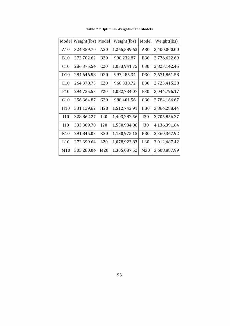
93

Table 7.7 Optimum Weights of the Models

Model Weight(lbs) Model Weight(lbs) Model Weight(lbs)

A10 324,359.70 A20 1,265,589.63 A30 3,400,000.00

B10 272,702.62 B20 998,232.87 B30 2,776,622.69

C10 286,375.54 C20 1,033,941.75 C30 2,823,142.45

D10 284,646.58 D20 997,485.34 D30 2,671,861.58

E10 264,378.75 E20 968,338.72 E30 2,723,415.28

F10 294,735.53 F20 1,082,734.07 F30 3,044,796.17

G10 256,364.87 G20 988,401.56 G30 2,784,166.67

H10 331,129.62 H20 1,512,742.91 H30 3,864,288.44

I10 328,862.27 I20 1,403,282.56 I30 3,705,856.27

J10 333,309.78 J20 1,550,934.86 J30 4,136,391.64

K10 291,845.03 K20 1,130,975.15 K30 3,360,367.92

L10 272,399.64 L20 1,078,923.83 L30 3,012,487.42

M10 305,280.04 M20 1,305,087.52 M30 3,608,887.99

Table 7.8 Cost of 10-Storey Models

Model Element Mass(kg)

Element Cost (Euro)

Joint Cost (Euro)

Transportation Cost (Euro)

Erection Cost (Euro)

Extra Costs (Euro)

Total Cost(Euro)

A-10 147,127.09 58,850.83 19,002.57 3,569.09 27,300.31 29,850.58 138,573.39 B-10 123,695.83 49,478.33 19,002.57 3,053.60 23,357.29 25,539.23 120,431.03 C-10 129,897.76 51,959.10 19,002.57 3,190.05 24,400.96 26,680.39 125,233.06 D-10 129,113.52 51,645.41 19,002.57 3,172.79 24,268.98 26,536.09 124,625.84 E-10 119,920.18 47,968.07 19,002.57 2,970.54 22,721.93 24,844.51 117,507.63 F-10 133,689.79 53,475.91 19,002.57 3,273.47 25,039.08 27,378.12 128,169.15 G-10 116,285.15 46,514.06 19,002.57 2,890.57 22,110.23 24,175.67 114,693.09 H-10 150,197.87 60,079.15 2,529.66 3,322.66 25,415.31 27,789.50 119,136.26 I-10 149,169.42 59,667.77 2,529.66 3,300.03 25,242.24 27,600.26 118,339.95 J-10 151,186.77 60,474.71 2,529.66 3,344.41 25,581.72 27,971.45 119,901.95 K-10 132,378.68 52,951.47 12,406.12 3,124.34 23,898.35 26,130.84 118,511.12 L-10 123,558.40 49,423.36 12,406.12 2,930.29 22,414.08 24,507.90 111,681.75 M-10 138,472.70 55,389.08 12,406.12 3,258.41 24,923.85 27,252.13 123,229.60

94

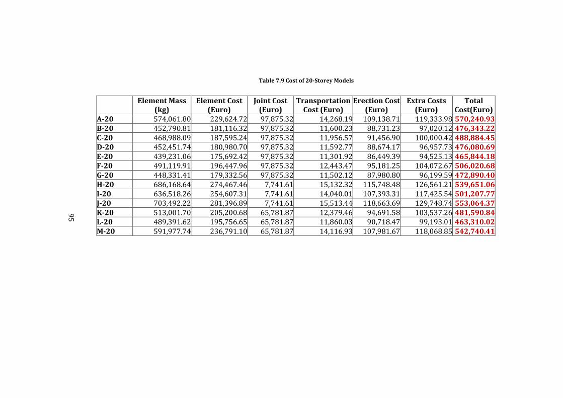
Table 7.9 Cost of 20-Storey Models

Element Mass(kg)

Element Cost (Euro)

Joint Cost (Euro)

Transportation Cost (Euro)

Erection Cost (Euro)

Extra Costs (Euro)

Total Cost(Euro)

A-20 574,061.80 229,624.72 97,875.32 14,268.19 109,138.71 119,333.98 570,240.93 B-20 452,790.81 181,116.32 97,875.32 11,600.23 88,731.23 97,020.12 476,343.22 C-20 468,988.09 187,595.24 97,875.32 11,956.57 91,456.90 100,000.42 488,884.45 D-20 452,451.74 180,980.70 97,875.32 11,592.77 88,674.17 96,957.73 476,080.69 E-20 439,231.06 175,692.42 97,875.32 11,301.92 86,449.39 94,525.13 465,844.18 F-20 491,119.91 196,447.96 97,875.32 12,443.47 95,181.25 104,072.67 506,020.68 G-20 448,331.41 179,332.56 97,875.32 11,502.12 87,980.80 96,199.59 472,890.40 H-20 686,168.64 274,467.46 7,741.61 15,132.32 115,748.48 126,561.21 539,651.06 I-20 636,518.26 254,607.31 7,741.61 14,040.01 107,393.31 117,425.54 501,207.77 J-20 703,492.22 281,396.89 7,741.61 15,513.44 118,663.69 129,748.74 553,064.37 K-20 513,001.70 205,200.68 65,781.87 12,379.46 94,691.58 103,537.26 481,590.84 L-20 489,391.62 195,756.65 65,781.87 11,860.03 90,718.47 99,193.01 463,310.02 M-20 591,977.74 236,791.10 65,781.87 14,116.93 107,981.67 118,068.85 542,740.41

95

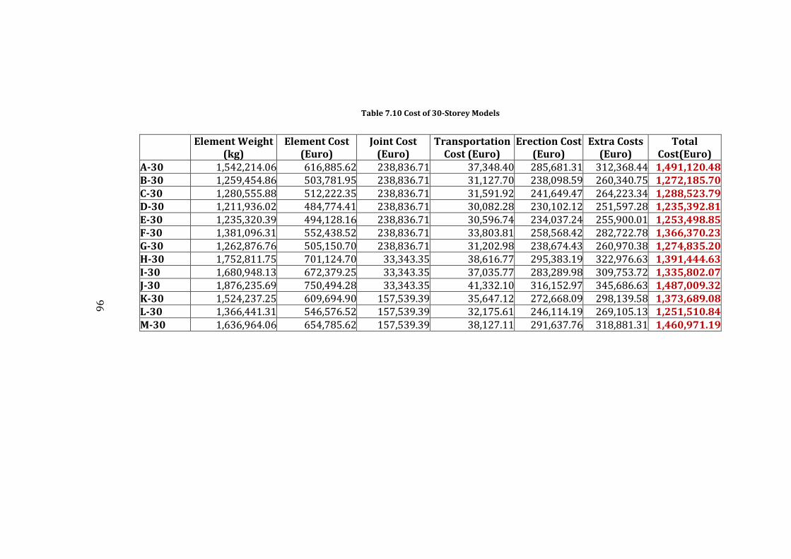
Table 7.10 Cost of 30-Storey Models

Element Weight(kg)

Element Cost(Euro)

Joint Cost(Euro)

Transportation Cost (Euro)

Erection Cost(Euro)

Extra Costs(Euro)

Total Cost(Euro)

A-30 1,542,214.06 616,885.62 238,836.71 37,348.40 285,681.31 312,368.44 1,491,120.48 B-30 1,259,454.86 503,781.95 238,836.71 31,127.70 238,098.59 260,340.75 1,272,185.70 C-30 1,280,555.88 512,222.35 238,836.71 31,591.92 241,649.47 264,223.34 1,288,523.79 D-30 1,211,936.02 484,774.41 238,836.71 30,082.28 230,102.12 251,597.28 1,235,392.81 E-30 1,235,320.39 494,128.16 238,836.71 30,596.74 234,037.24 255,900.01 1,253,498.85 F-30 1,381,096.31 552,438.52 238,836.71 33,803.81 258,568.42 282,722.78 1,366,370.23 G-30 1,262,876.76 505,150.70 238,836.71 31,202.98 238,674.43 260,970.38 1,274,835.20 H-30 1,752,811.75 701,124.70 33,343.35 38,616.77 295,383.19 322,976.63 1,391,444.63 I-30 1,680,948.13 672,379.25 33,343.35 37,035.77 283,289.98 309,753.72 1,335,802.07 J-30 1,876,235.69 750,494.28 33,343.35 41,332.10 316,152.97 345,686.63 1,487,009.32 K-30 1,524,237.25 609,694.90 157,539.39 35,647.12 272,668.09 298,139.58 1,373,689.08 L-30 1,366,441.31 546,576.52 157,539.39 32,175.61 246,114.19 269,105.13 1,251,510.84 M-30 1,636,964.06 654,785.62 157,539.39 38,127.11 291,637.76 318,881.31 1,460,971.19

96

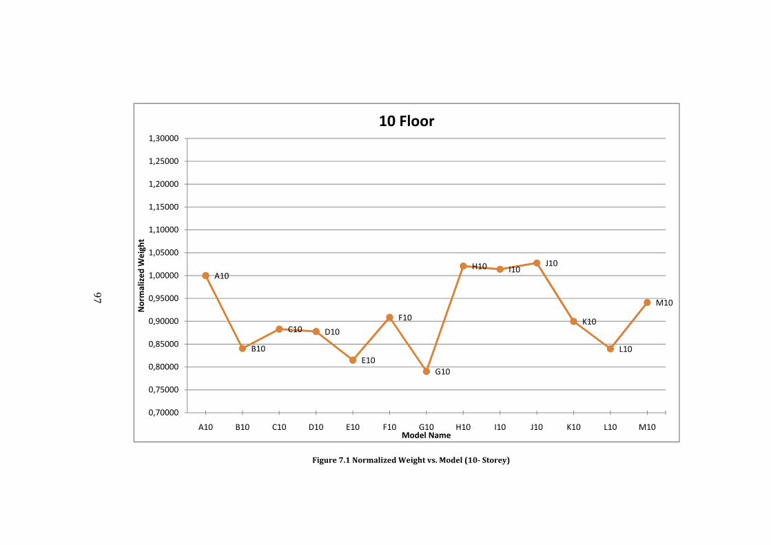
Figure 7.1 Normalized Weight vs. Model (10- Storey)

97

A10

B10

C10 D10

E10

F10

G10

H10 I10J10

K10

L10

M10

0,70000

0,75000

0,80000

0,85000

0,90000

0,95000

1,00000

1,05000

1,10000

1,15000

1,20000

1,25000

1,30000

A10 B10 C10 D10 E10 F10 G10 H10 I10 J10 K10 L10 M10

Nor

mal

ized

Wei

ght

Model Name

10 Floor

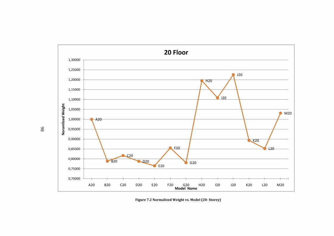
Figure 7.2 Normalized Weight vs. Model (20- Storey)

98

A20

B20C20

D20E20

F20

G20

H20

I20

J20

K20

L20

M20

0,70000

0,75000

0,80000

0,85000

0,90000

0,95000

1,00000

1,05000

1,10000

1,15000

1,20000

1,25000

1,30000

A20 B20 C20 D20 E20 F20 G20 H20 I20 J20 K20 L20 M20

Nor

amliz

ed W

eigh

t

Model Name

20 Floor

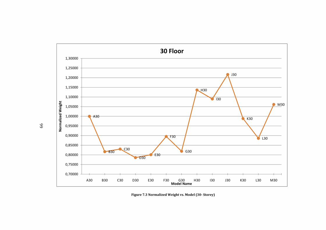
Figure 7.3 Normalized Weight vs. Model (30- Storey)

99

A30

B30C30

D30E30

F30

G30

H30

I30

J30

K30

L30

M30

0,70000

0,75000

0,80000

0,85000

0,90000

0,95000

1,00000

1,05000

1,10000

1,15000

1,20000

1,25000

1,30000

A30 B30 C30 D30 E30 F30 G30 H30 I30 J30 K30 L30 M30

Nor

mal

ized

Wei

ght

Model Name

30 Floor

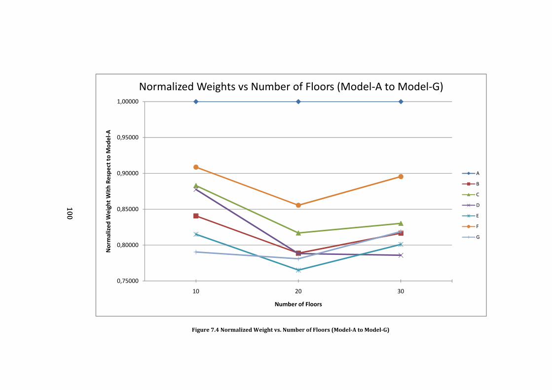
Figure 7.4 Normalized Weight vs. Number of Floors (Model-A to Model-G)

100100

0,75000

0,80000

0,85000

0,90000

0,95000

1,00000

10 20 30

Nor

mal

ized

Wei

ght W

ith R

espe

ct to

Mod

el-A

Number of Floors

Normalized Weights vs Number of Floors (Model-A to Model-G)

A

B

C

D

E

F

G

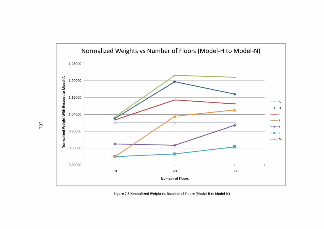
Figure 7.5 Normalized Weight vs. Number of Floors (Model-H to Model-N)

101

0,80000

0,88000

0,96000

1,04000

1,12000

1,20000

1,28000

10 20 30

Nor

mal

ized

Wei

ght W

ith R

espe

ct to

Mod

el-A

Number of Floors

Normalized Weights vs Number of Floors (Model-H to Model-N)

A

H

I

J

K

L

M

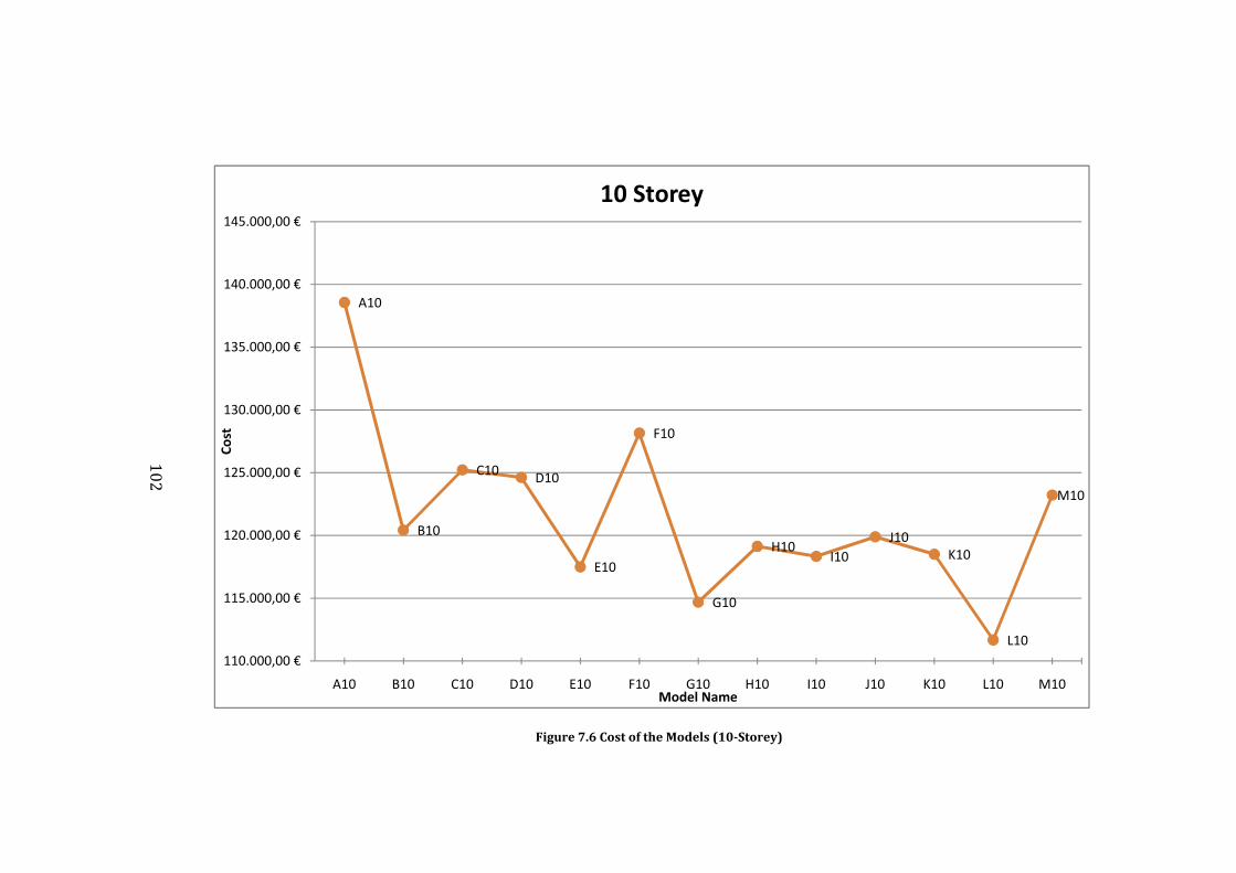
Figure 7.6 Cost of the Models (10-Storey)

102

A10

B10

C10 D10

E10

F10

G10

H10I10

J10K10

L10

M10

110.000,00 €

115.000,00 €

120.000,00 €

125.000,00 €

130.000,00 €

135.000,00 €

140.000,00 €

145.000,00 €

A10 B10 C10 D10 E10 F10 G10 H10 I10 J10 K10 L10 M10

Cost

Model Name

10 Storey

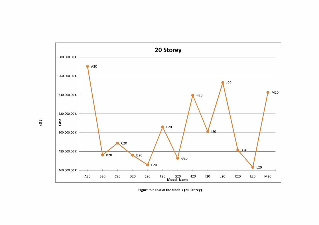
Figure 7.7 Cost of the Models (20-Storey)

103

A20

B20

C20

D20

E20

F20

G20

H20

I20

J20

K20

L20

M20

460.000,00 €

480.000,00 €

500.000,00 €

520.000,00 €

540.000,00 €

560.000,00 €

580.000,00 €

A20 B20 C20 D20 E20 F20 G20 H20 I20 J20 K20 L20 M20

Cost

Model Name

20 Storey

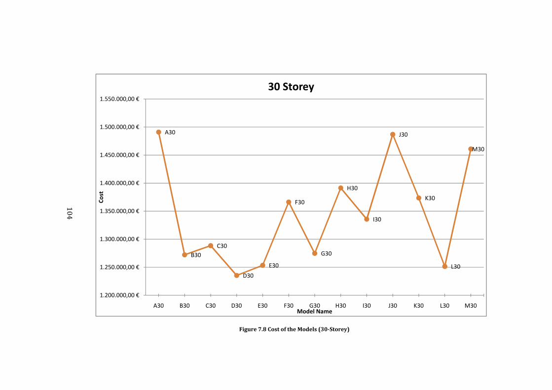
Figure 7.8 Cost of the Models (30-Storey)

104

A30

B30C30

D30

E30

F30

G30

H30

I30

J30

K30

L30

M30

1.200.000,00 €

1.250.000,00 €

1.300.000,00 €

1.350.000,00 €

1.400.000,00 €

1.450.000,00 €

1.500.000,00 €

1.550.000,00 €

A30 B30 C30 D30 E30 F30 G30 H30 I30 J30 K30 L30 M30

Cost

Model Name

30 Storey

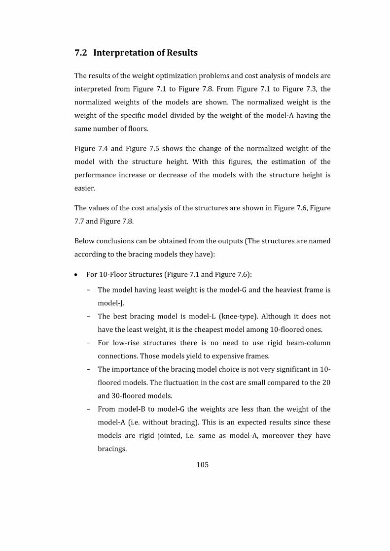
105

7.2 Interpretation of Results

The results of the weight optimization problems and cost analysis of models are

interpreted from Figure 7.1 to Figure 7.8. From Figure 7.1 to Figure 7.3, the

normalized weights of the models are shown. The normalized weight is the

weight of the specific model divided by the weight of the model-A having the

same number of floors.

Figure 7.4 and Figure 7.5 shows the change of the normalized weight of the

model with the structure height. With this figures, the estimation of the

performance increase or decrease of the models with the structure height is

easier.

The values of the cost analysis of the structures are shown in Figure 7.6, Figure

7.7 and Figure 7.8.

Below conclusions can be obtained from the outputs (The structures are named

according to the bracing models they have):

For 10-Floor Structures (Figure 7.1 and Figure 7.6):

- The model having least weight is the model-G and the heaviest frame is

model-J.

- The best bracing model is model-L (knee-type). Although it does not

have the least weight, it is the cheapest model among 10-floored ones.

- For low-rise structures there is no need to use rigid beam-column

connections. Those models yield to expensive frames.

- The importance of the bracing model choice is not very significant in 10-

floored models. The fluctuation in the cost are small compared to the 20

and 30-floored models.

- From model-B to model-G the weights are less than the weight of the

model-A (i.e. without bracing). This is an expected results since these

models are rigid jointed, i.e. same as model-A, moreover they have

bracings.

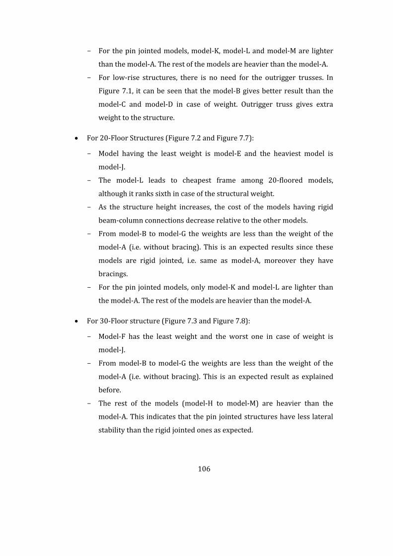
106

- For the pin jointed models, model-K, model-L and model-M are lighter

than the model-A. The rest of the models are heavier than the model-A.

- For low-rise structures, there is no need for the outrigger trusses. In

Figure 7.1, it can be seen that the model-B gives better result than the

model-C and model-D in case of weight. Outrigger truss gives extra

weight to the structure.

For 20-Floor Structures (Figure 7.2 and Figure 7.7):

- Model having the least weight is model-E and the heaviest model is

model-J.

- The model-L leads to cheapest frame among 20-floored models,

although it ranks sixth in case of the structural weight.

- As the structure height increases, the cost of the models having rigid

beam-column connections decrease relative to the other models.

- From model-B to model-G the weights are less than the weight of the

model-A (i.e. without bracing). This is an expected results since these

models are rigid jointed, i.e. same as model-A, moreover they have

bracings.

- For the pin jointed models, only model-K and model-L are lighter than

the model-A. The rest of the models are heavier than the model-A.

For 30-Floor structure (Figure 7.3 and Figure 7.8):

- Model-F has the least weight and the worst one in case of weight is

model-J.

- From model-B to model-G the weights are less than the weight of the

model-A (i.e. without bracing). This is an expected result as explained

before.

- The rest of the models (model-H to model-M) are heavier than the

model-A. This indicates that the pin jointed structures have less lateral

stability than the rigid jointed ones as expected.

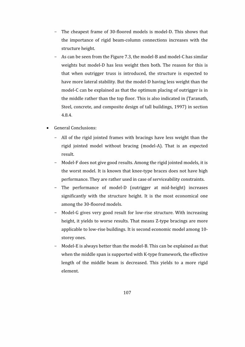
107

- The cheapest frame of 30-floored models is model-D. This shows that

the importance of rigid beam-column connections increases with the

structure height.

- As can be seen from the Figure 7.3, the model-B and model-C has similar

weights but model-D has less weight then both. The reason for this is

that when outrigger truss is introduced, the structure is expected to

have more lateral stability. But the model-D having less weight than the

model-C can be explained as that the optimum placing of outrigger is in

the middle rather than the top floor. This is also indicated in (Taranath,

Steel, concrete, and composite design of tall buildings, 1997) in section

4.8.4.

General Conclusions:

- All of the rigid jointed frames with bracings have less weight than the

rigid jointed model without bracing (model-A). That is an expected

result.

- Model-F does not give good results. Among the rigid jointed models, it is

the worst model. It is known that knee-type braces does not have high

performance. They are rather used in case of serviceability constraints.

- The performance of model-D (outrigger at mid-height) increases

significantly with the structure height. It is the most economical one

among the 30-floored models.

- Model-G gives very good result for low-rise structure. With increasing

height, it yields to worse results. That means Z-type bracings are more

applicable to low-rise buildings. It is second economic model among 10-

storey ones.

- Model-E is always better than the model-B. This can be explained as that

when the middle span is supported with K-type framework, the effective

length of the middle beam is decreased. This yields to a more rigid

element.

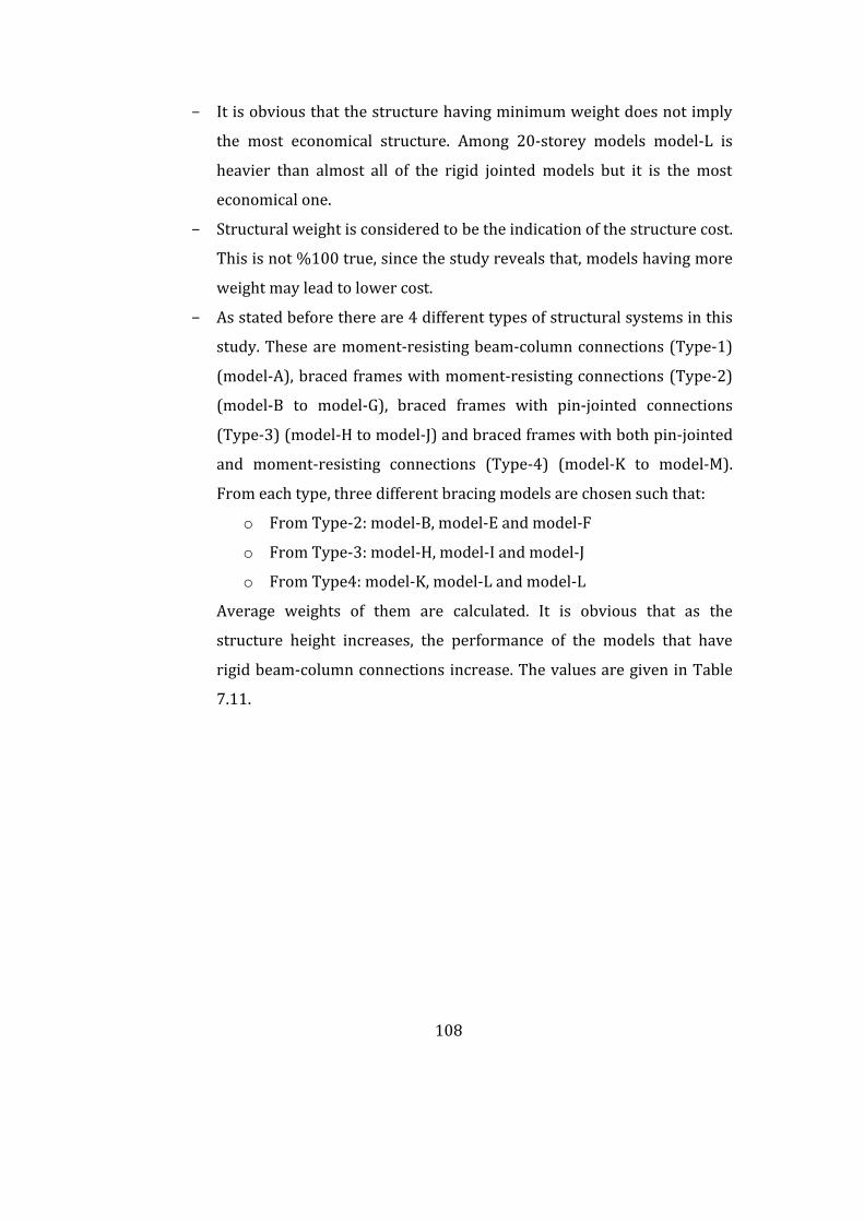
108

- It is obvious that the structure having minimum weight does not imply

the most economical structure. Among 20-storey models model-L is

heavier than almost all of the rigid jointed models but it is the most

economical one.

- Structural weight is considered to be the indication of the structure cost.

This is not %100 true, since the study reveals that, models having more

weight may lead to lower cost.

- As stated before there are 4 different types of structural systems in this

study. These are moment-resisting beam-column connections (Type-1)

(model-A), braced frames with moment-resisting connections (Type-2)

(model-B to model-G), braced frames with pin-jointed connections

(Type-3) (model-H to model-J) and braced frames with both pin-jointed

and moment-resisting connections (Type-4) (model-K to model-M).

From each type, three different bracing models are chosen such that:

o From Type-2: model-B, model-E and model-F

o From Type-3: model-H, model-I and model-J

o From Type4: model-K, model-L and model-L

Average weights of them are calculated. It is obvious that as the

structure height increases, the performance of the models that have

rigid beam-column connections increase. The values are given in Table

7.11.

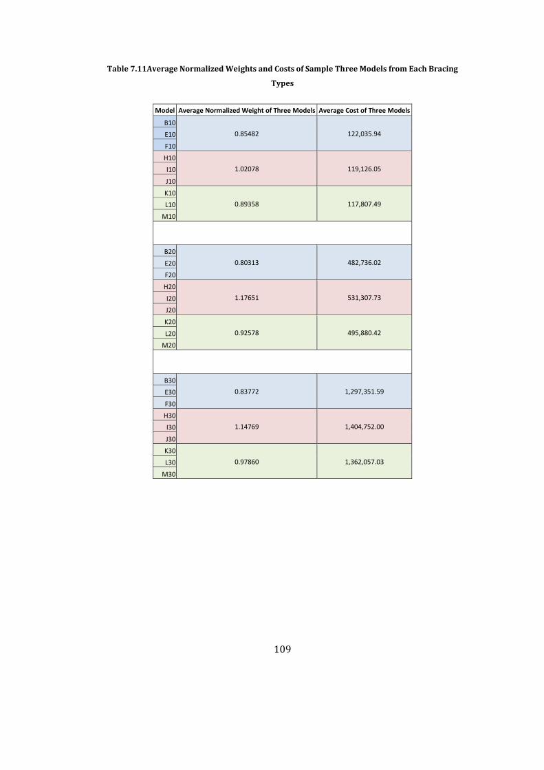
109

Table 7.11Average Normalized Weights and Costs of Sample Three Models from Each Bracing

Types

Model Average Normalized Weight of Three Models Average Cost of Three Models

B100.85482 122,035.94E10

F10

H101.02078 119,126.05I10

J10

K100.89358 117,807.49L10

M10

B200.80313 482,736.02E20

F20

H201.17651 531,307.73I20

J20

K200.92578 495,880.42L20

M20

B300.83772 1,297,351.59E30

F30

H301.14769 1,404,752.00I30

J30

K300.97860 1,362,057.03L30

M30

110

Chapter 8

CONCLUSIONS AND SUMMARY

Since the design of structures is a challenging task, not all the designers can

manage to make a perfect or optimum design. This yields to non-economical

structures since the sections that are used are larger than they supposed to be.

Since economy is one of the most important considerations of the design

process, designers should find a way of making more economical designs. This

is possible only if he/she uses some optimization techniques.

The main starting point of the ESs is to solve problems that have real-valued

parameter. After some time, ESs were developed to solve problems that has

discrete parameters. For a structural design problem, there is definite number

of members and there is generally a steel set of sections that the designer

chooses from. This is a typical example of a problem having discrete

parameters.

The aim of this study is to determine the optimal configuration of lateral

bracing models in steel structures subjected to wind forces. For this purpose

three different structures (10, 20 and 30 floored) are prepared and optimum

designs of them with twelve different bracing models are carried out. The wind

speed is assumed to be 125 mph and as a lateral load, only wind load is taken

into consideration. In case of having other types of loads like earthquake loads,

the performances of the models might change slightly. For all design examples,

111

the following material properties of the steel are used: modulus of elasticity (E)

= 29,000 ksi (203,893.6 MPa) and yield stress ( yF ) = 36 ksi (253.1 MPa). The

detailed results and their discussions are given in Chapter 7.

General conclusions of the results are as below:

- Bracing always decreases the weight

- For low-rise structures, there is no need to use rigid connections

- For low-rise structures, the bracing choice is not very important

- There is no need for an outrigger truss in low-rise models

- Z-type bracings are more applicable to low-rise structures

- Model having a high weight may lead to a low-cost model. Typical

example to this case is L-20

- Pin-jointed structures are always heavier than the rigid jointed ones

- Importance of the rigid connections increases with the structure height

- Knee-type bracing does not give good results. We only consider of using

this type of bracing when there is space limitation

Summary of the thesis is given below:

In Chapter 2, the optimum design of steel frames is explained. First,

optimization is explained. Details of it is given. Then the design optimization of

steel frames is given and problem formulation is indicated. The constraints of

the problem are given in this chapter also. Evolutionary Algorithms is explained

and then detailed description of the ESs is given. The step-by-step procedure of

ESs is introduced. Then the operators of it such as recombination and mutation

are explained. The differences between continuous and discrete approaches are

outlined in this chapter also.

In Chapter 3, design loads that are used on the test structures are outlined.

There are mainly four load types that are used in our structures. As gravity

loads; dead load, live load and snow load are applied. On the other hand, as the

horizontal force the wind loads are chosen. In this chapter, calculations of these

112

loads are given in detail. First the wind loads are explained. The importance of

wind loads on structures is given. After that the step-by-step procedure of the

wind load calculation is outlined according to ASCE 7 method 2. The wind

loading values of the structures are presented in tables. After that the dead, live

and snow load calculations are given and the values of them are tabulated.

In Chapter 4, the lateral force resisting systems are outlined. The reason for the

usage of bracing systems in structures is given. After that the bracing models in

the literature are introduced. There are mainly four types of systems that are

used in our study: (i) moment-resisting beam-column connections, (ii) braced

frames with moment-resisting connections, (iii) braced frames with pin-jointed

connections and (iv) braced frames with both pin-jointed and moment-

resisting connections. These systems with different brace arrangements like x-

type, z-type, k-type are studied in this study.

In Chapter 5 cost analysis of steel frames is described. In many cases, structure

with best design weight is pretended to be the most economic one. However,

this is only an assumption that the minimal weight could lead to reasonable low

overall costs. Other costs such as joint costs can differ from structure to

structure such that it can affect the total cost significantly. Here, in this chapter

cost of a structure is divided in to five parts. These are total material cost of the

elements, total material and manufacturing cost of joints, total transportation

costs, total erection costs and extra costs. Cost of the structure can be defined

as the sum of all these four elements.

In Chapter 6 the details of the structural models are given. Three different

structures with 10, 20 and 30 stories are considered and for every structure all

of the prescribed bracing models are applied. Members are grouped such that

inner beams, outer beams, corner columns, x-z outer columns, y-z outer

columns, inner columns and bracing members at every two floors have the

same cross-section. There are two load cases. In the first load case, the gravity

113

loads are applied with the wind loads acting along x-axis, in the second one

they are applied with the wind forces acting along y-axis.

As stated before the results of the analyses and discussions are given in Chapter

7.

114

REFERENCES

AISC. (1989). Manual Of Steel Construction, Allowable Stress Design, 9th Adition.

Algor. (2009, 07 18). Retrieved 07 18, 2009, from Algor: http://www.algor.com

ANSI/AISC, 3.-0. (2005). Specifications For Structural Steel Buildings. Chicago:

AMERICAN INSTITUTE OF STEEL CONSTRUCTION.

ASCE. (2006). Minimum Design Loads for Buildings and Other Structures. Reston:

American Society of civil Engineers.

Bäck, T. (1996). Evolutionary Algorithms In Theory and Practice. New York:

Oxford University Press.

Brockenbrough, R. L., & Merritt, F. S. (2005). Structural Steel Designer's

Handbook: AISC, AASHTO, AISI, ASTM, AREMA, and ASCE-07 Design Standards.

McGraw-Hill Professional.

Dumitrescu, D., Lazzerini, b., Jain, L. C., & Dumitrescu, A. (2000). Evolutionary

Computation. Florida: CRC Press.

Eiben, A. E., & Smith, J. E. (1998). Introduction to Evolutionary Computing. New

York: Springer.

ESDEP. (2009, 07 16). Retrieved 07 16, 2009, from ESDEP: http://www.fgg.uni-

lj.si/

Haftka, R. T., & Gürdal, Z. (1991). Elements of structural optimization. Springer.

115

Hasançebi, O. (2008). Adaptive evolution strategies in structural optimization:

Enhancing their computational performance with applications to large-scale

structures. Computers and Structures , 119-132.

Hasançebi, O. (2007). Discrete approaches in evolution strategies based

optimum design of steel frames. Structural Engineering and Mechanics , 191-

210.

Hasançebi, O. (2007). Optimization of truss bridges within a specified design

domain using evolution strategies. Engineering Optimization , 737-756.

Hasançebi, O., Çarbaş, S., Doğan, E., Erdal, F., & Saka, M. P. (2009). Performance

evaluation of metaheuristic search techniques in the optimum design of real

size pin jointed structures. Computers and Structures , 284-302.

Holmes, J. D. (2001). Wind Loading of Structures. Taylor and Francis.

IDEERS Resistant Buildings. (n.d.). Retrieved 07 16, 2009, from

http://www.ideers.bris.ac.uk

Kameshki, E. S., & Saka, M. P. (2001). Genetic algorithm based optimum bracing

design of non-swaying tall plane frames. Journal of Constructional Steel

Research , 1081-1097.

Mehta, K. C., & Delahay, J. (2003). Guide to the use of the wind load provisions of

ASCE 7-02. ASCE Publications.

Memari, A. M., & Madhkhan, M. (1999). Optimal design of steel frames subject

to gravity and seismic codes' prescribed lateral forces. Structural Optimization ,

56-66.

Papadrakakis, M., Lagaros, N. D., & Tsompanakis, Y. (1998). Structural

Optimization Using Evolution Strategies and Neural Networks. Comput.

Methods Appl. Mech. Engrg. , 309-333.

116

Pavlovic, L., Krajnc, A., & Beg, D. (2004). Cost function analysis in the structural

optimization of steel frames. Struct. Multidisc. Optim. , 286-295.

Runarsson, T. P., & Yao, X. (2002). Continuous Selection and Self-Adaptive

Evolution Strategies. Evolutionary Computation, 2002. CEC '02. Proceedings of

the 2002 Congress , I, 279-284.

Sputo, T., & Turner, J. L. (2006). Bracing cold-formed steel structures: a design

guide. ASCE Publications.

Taranath, B. S. (1997). Steel, concrete, and composite design of tall buildings.

McGraw-Hill Professional.

Taranath, B. S. (2005). Wind and Earthquake Resistant Buildings. Florida:

Taylor&Francis Group.

Topologica Solutions. (2009, 07 18). Retrieved 07 18, 2009, from Topologica

Solutions: http://www.topologicasolutions.com

117

APPENDIX A

OVERVIEW OF THE SOFTWARE, OPTSTEEL

The optimization software is called OPTSTEEL, Optimum Design of Steel

Structural Systems in Parallel Computing Environment, designed by Dr. O.

Hasançebi from Middle East Technical University.

OPTSTEEL is software capable of making the optimal design of a structure

using Evolution Strategies, which is one of the techniques of Evolutionary

Algorithms. The main screen of the software can be seen in Figure A-1:

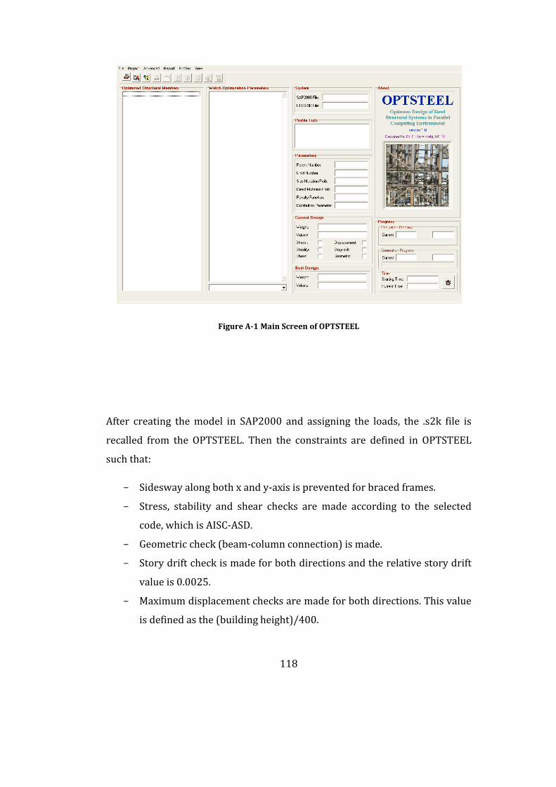
118

Figure A-1 Main Screen of OPTSTEEL

After creating the model in SAP2000 and assigning the loads, the .s2k file is

recalled from the OPTSTEEL. Then the constraints are defined in OPTSTEEL

such that:

- Sidesway along both x and y-axis is prevented for braced frames.

- Stress, stability and shear checks are made according to the selected

code, which is AISC-ASD.

- Geometric check (beam-column connection) is made.

- Story drift check is made for both directions and the relative story drift

value is 0.0025.

- Maximum displacement checks are made for both directions. This value

is defined as the (building height)/400.

119

For the computational time advantages, the structural analyses are made in

SAP2000. The software is automated to interact with SAP2000 v7.4 structural

analysis program for generating and screening the structural models of the

problems under consideration as well as carrying out a displacement based

finite element analysis for each solution sampled during optimization process.

Therefore the models of the structures are created in SAP2000. Some screen

shots of SAP-models can be seen in Figure A-2 and Figure A-3.

120

Figure A-2 10-Storey Model 3-D View

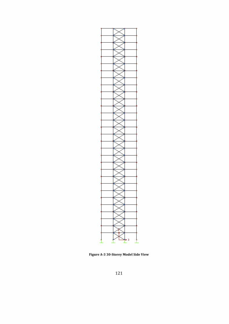
121

Figure A-3 30-Storey Model Side View

122

After creating the model, assigning initial sections to the members and defining

the loads, the .s2k file is opened from OPTSTEEL (Figure A-4).

Figure A-4 Open SAP2000 Input File Screen of OPTSTEEL

Since this is an optimization software, the program needs some information of

sections and their orientations from which it can selects and makes analysis

with different combinations. From the define data section, the member profiles,

their orientations and some other parameters can be defined. Here in Figure

A-5 and Figure A-6, the member grouping file created before is recalled from

“Define Data” section so that the members, that we want to be the same, are

grouped and the software selects same steel section for all of the members of a

group.

123

Figure A-5 “Open Grouping File” Screen of OPTSTEEL

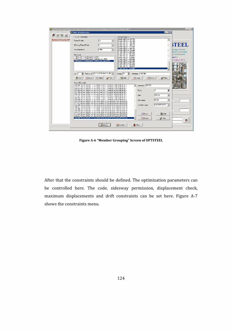
124

Figure A-6 “Member Grouping” Screen of OPTSTEEL

After that the constraints should be defined. The optimization parameters can

be controlled here. The code, sidesway permission, displacement check,

maximum displacements and drift constraints can be set here. Figure A-7

shows the constraints menu.

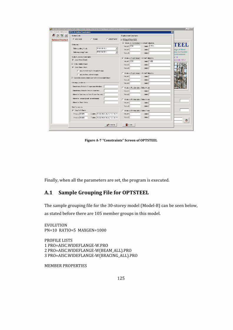
125

Figure A-7 “Constraints” Screen of OPTSTEEL

Finally, when all the parameters are set, the program is executed.

A.1 Sample Grouping File for OPTSTEEL

The sample grouping file for the 30-storey model (Model-B) can be seen below,

as stated before there are 105 member groups in this model.

EVOLUTIONPN=10 RATIO=5 MAXGEN=1000

PROFILE LISTS1 PRO=AISC.WIDEFLANGE-W.PRO2 PRO=AISC.WIDEFLANGE-W(BEAM_ALL).PRO3 PRO=AISC.WIDEFLANGE-W(BRACING_ALL).PRO

MEMBER PROPERTIES

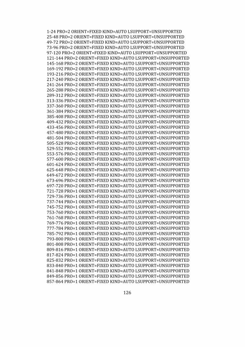
126

1-24 PRO=2 ORIENT=FIXED KIND=AUTO LSUPPORT=UNSUPPORTED25-48 PRO=2 ORIENT=FIXED KIND=AUTO LSUPPORT=UNSUPPORTED49-72 PRO=2 ORIENT=FIXED KIND=AUTO LSUPPORT=UNSUPPORTED73-96 PRO=2 ORIENT=FIXED KIND=AUTO LSUPPORT=UNSUPPORTED97-120 PRO=2 ORIENT=FIXED KIND=AUTO LSUPPORT=UNSUPPORTED121-144 PRO=2 ORIENT=FIXED KIND=AUTO LSUPPORT=UNSUPPORTED145-168 PRO=2 ORIENT=FIXED KIND=AUTO LSUPPORT=UNSUPPORTED169-192 PRO=2 ORIENT=FIXED KIND=AUTO LSUPPORT=UNSUPPORTED193-216 PRO=2 ORIENT=FIXED KIND=AUTO LSUPPORT=UNSUPPORTED217-240 PRO=2 ORIENT=FIXED KIND=AUTO LSUPPORT=UNSUPPORTED241-264 PRO=2 ORIENT=FIXED KIND=AUTO LSUPPORT=UNSUPPORTED265-288 PRO=2 ORIENT=FIXED KIND=AUTO LSUPPORT=UNSUPPORTED289-312 PRO=2 ORIENT=FIXED KIND=AUTO LSUPPORT=UNSUPPORTED313-336 PRO=2 ORIENT=FIXED KIND=AUTO LSUPPORT=UNSUPPORTED337-360 PRO=2 ORIENT=FIXED KIND=AUTO LSUPPORT=UNSUPPORTED361-384 PRO=2 ORIENT=FIXED KIND=AUTO LSUPPORT=UNSUPPORTED385-408 PRO=2 ORIENT=FIXED KIND=AUTO LSUPPORT=UNSUPPORTED409-432 PRO=2 ORIENT=FIXED KIND=AUTO LSUPPORT=UNSUPPORTED433-456 PRO=2 ORIENT=FIXED KIND=AUTO LSUPPORT=UNSUPPORTED457-480 PRO=2 ORIENT=FIXED KIND=AUTO LSUPPORT=UNSUPPORTED481-504 PRO=2 ORIENT=FIXED KIND=AUTO LSUPPORT=UNSUPPORTED505-528 PRO=2 ORIENT=FIXED KIND=AUTO LSUPPORT=UNSUPPORTED529-552 PRO=2 ORIENT=FIXED KIND=AUTO LSUPPORT=UNSUPPORTED553-576 PRO=2 ORIENT=FIXED KIND=AUTO LSUPPORT=UNSUPPORTED577-600 PRO=2 ORIENT=FIXED KIND=AUTO LSUPPORT=UNSUPPORTED601-624 PRO=2 ORIENT=FIXED KIND=AUTO LSUPPORT=UNSUPPORTED625-648 PRO=2 ORIENT=FIXED KIND=AUTO LSUPPORT=UNSUPPORTED649-672 PRO=2 ORIENT=FIXED KIND=AUTO LSUPPORT=UNSUPPORTED673-696 PRO=2 ORIENT=FIXED KIND=AUTO LSUPPORT=UNSUPPORTED697-720 PRO=2 ORIENT=FIXED KIND=AUTO LSUPPORT=UNSUPPORTED721-728 PRO=1 ORIENT=FIXED KIND=AUTO LSUPPORT=UNSUPPORTED729-736 PRO=1 ORIENT=FIXED KIND=AUTO LSUPPORT=UNSUPPORTED737-744 PRO=1 ORIENT=FIXED KIND=AUTO LSUPPORT=UNSUPPORTED745-752 PRO=1 ORIENT=FIXED KIND=AUTO LSUPPORT=UNSUPPORTED753-760 PRO=1 ORIENT=FIXED KIND=AUTO LSUPPORT=UNSUPPORTED761-768 PRO=1 ORIENT=FIXED KIND=AUTO LSUPPORT=UNSUPPORTED769-776 PRO=1 ORIENT=FIXED KIND=AUTO LSUPPORT=UNSUPPORTED777-784 PRO=1 ORIENT=FIXED KIND=AUTO LSUPPORT=UNSUPPORTED785-792 PRO=1 ORIENT=FIXED KIND=AUTO LSUPPORT=UNSUPPORTED793-800 PRO=1 ORIENT=FIXED KIND=AUTO LSUPPORT=UNSUPPORTED801-808 PRO=1 ORIENT=FIXED KIND=AUTO LSUPPORT=UNSUPPORTED809-816 PRO=1 ORIENT=FIXED KIND=AUTO LSUPPORT=UNSUPPORTED817-824 PRO=1 ORIENT=FIXED KIND=AUTO LSUPPORT=UNSUPPORTED825-832 PRO=1 ORIENT=FIXED KIND=AUTO LSUPPORT=UNSUPPORTED833-840 PRO=1 ORIENT=FIXED KIND=AUTO LSUPPORT=UNSUPPORTED841-848 PRO=1 ORIENT=FIXED KIND=AUTO LSUPPORT=UNSUPPORTED849-856 PRO=1 ORIENT=FIXED KIND=AUTO LSUPPORT=UNSUPPORTED857-864 PRO=1 ORIENT=FIXED KIND=AUTO LSUPPORT=UNSUPPORTED

127

865-872 PRO=1 ORIENT=FIXED KIND=AUTO LSUPPORT=UNSUPPORTED873-880 PRO=1 ORIENT=FIXED KIND=AUTO LSUPPORT=UNSUPPORTED881-888 PRO=1 ORIENT=FIXED KIND=AUTO LSUPPORT=UNSUPPORTED889-896 PRO=1 ORIENT=FIXED KIND=AUTO LSUPPORT=UNSUPPORTED897-904 PRO=1 ORIENT=FIXED KIND=AUTO LSUPPORT=UNSUPPORTED905-912 PRO=1 ORIENT=FIXED KIND=AUTO LSUPPORT=UNSUPPORTED913-920 PRO=1 ORIENT=FIXED KIND=AUTO LSUPPORT=UNSUPPORTED921-928 PRO=1 ORIENT=FIXED KIND=AUTO LSUPPORT=UNSUPPORTED929-936 PRO=1 ORIENT=FIXED KIND=AUTO LSUPPORT=UNSUPPORTED937-944 PRO=1 ORIENT=FIXED KIND=AUTO LSUPPORT=UNSUPPORTED945-952 PRO=1 ORIENT=FIXED KIND=AUTO LSUPPORT=UNSUPPORTED953-960 PRO=1 ORIENT=FIXED KIND=AUTO LSUPPORT=UNSUPPORTED961-968 PRO=1 ORIENT=FIXED KIND=AUTO LSUPPORT=UNSUPPORTED969-976 PRO=1 ORIENT=FIXED KIND=AUTO LSUPPORT=UNSUPPORTED977-984 PRO=1 ORIENT=FIXED KIND=AUTO LSUPPORT=UNSUPPORTED985-992 PRO=1 ORIENT=FIXED KIND=AUTO LSUPPORT=UNSUPPORTED993-1000 PRO=1 ORIENT=FIXED KIND=AUTO LSUPPORT=UNSUPPORTED1001-1008 PRO=1 ORIENT=FIXED KIND=AUTO LSUPPORT=UNSUPPORTED1009-1016 PRO=1 ORIENT=FIXED KIND=AUTO LSUPPORT=UNSUPPORTED1017-1024 PRO=1 ORIENT=FIXED KIND=AUTO LSUPPORT=UNSUPPORTED1025-1032 PRO=1 ORIENT=FIXED KIND=AUTO LSUPPORT=UNSUPPORTED1033-1040 PRO=1 ORIENT=FIXED KIND=AUTO LSUPPORT=UNSUPPORTED1041-1048 PRO=1 ORIENT=FIXED KIND=AUTO LSUPPORT=UNSUPPORTED1049-1056 PRO=1 ORIENT=FIXED KIND=AUTO LSUPPORT=UNSUPPORTED1057-1064 PRO=1 ORIENT=FIXED KIND=AUTO LSUPPORT=UNSUPPORTED1065-1072 PRO=1 ORIENT=FIXED KIND=AUTO LSUPPORT=UNSUPPORTED1073-1080 PRO=1 ORIENT=FIXED KIND=AUTO LSUPPORT=UNSUPPORTED1081-1088 PRO=1 ORIENT=FIXED KIND=AUTO LSUPPORT=UNSUPPORTED1089-1096 PRO=1 ORIENT=FIXED KIND=AUTO LSUPPORT=UNSUPPORTED1097-1104 PRO=1 ORIENT=FIXED KIND=AUTO LSUPPORT=UNSUPPORTED1105-1112 PRO=1 ORIENT=FIXED KIND=AUTO LSUPPORT=UNSUPPORTED1113-1120 PRO=1 ORIENT=FIXED KIND=AUTO LSUPPORT=UNSUPPORTED1121-1128 PRO=1 ORIENT=FIXED KIND=AUTO LSUPPORT=UNSUPPORTED1129-1136 PRO=1 ORIENT=FIXED KIND=AUTO LSUPPORT=UNSUPPORTED1137-1144 PRO=1 ORIENT=FIXED KIND=AUTO LSUPPORT=UNSUPPORTED1145-1152 PRO=1 ORIENT=FIXED KIND=AUTO LSUPPORT=UNSUPPORTED1153-1160 PRO=1 ORIENT=FIXED KIND=AUTO LSUPPORT=UNSUPPORTED1161-1168 PRO=1 ORIENT=FIXED KIND=AUTO LSUPPORT=UNSUPPORTED1169-1176 PRO=1 ORIENT=FIXED KIND=AUTO LSUPPORT=UNSUPPORTED1177-1184 PRO=1 ORIENT=FIXED KIND=AUTO LSUPPORT=UNSUPPORTED1185-1192 PRO=1 ORIENT=FIXED KIND=AUTO LSUPPORT=UNSUPPORTED1193-1200 PRO=1 ORIENT=FIXED KIND=AUTO LSUPPORT=UNSUPPORTED1201-1216 PRO=3 ORIENT=FIXED KIND=TRUSS LSUPPORT=UNSUPPORTED1217-1232 PRO=3 ORIENT=FIXED KIND=TRUSS LSUPPORT=UNSUPPORTED1233-1248 PRO=3 ORIENT=FIXED KIND=TRUSS LSUPPORT=UNSUPPORTED1249-1264 PRO=3 ORIENT=FIXED KIND=TRUSS LSUPPORT=UNSUPPORTED1265-1280 PRO=3 ORIENT=FIXED KIND=TRUSS LSUPPORT=UNSUPPORTED1281-1296 PRO=3 ORIENT=FIXED KIND=TRUSS LSUPPORT=UNSUPPORTED

128

1297-1312 PRO=3 ORIENT=FIXED KIND=TRUSS LSUPPORT=UNSUPPORTED1313-1328 PRO=3 ORIENT=FIXED KIND=TRUSS LSUPPORT=UNSUPPORTED1329-1344 PRO=3 ORIENT=FIXED KIND=TRUSS LSUPPORT=UNSUPPORTED1345-1360 PRO=3 ORIENT=FIXED KIND=TRUSS LSUPPORT=UNSUPPORTED1361-1376 PRO=3 ORIENT=FIXED KIND=TRUSS LSUPPORT=UNSUPPORTED1377-1392 PRO=3 ORIENT=FIXED KIND=TRUSS LSUPPORT=UNSUPPORTED1393-1408 PRO=3 ORIENT=FIXED KIND=TRUSS LSUPPORT=UNSUPPORTED1409-1424 PRO=3 ORIENT=FIXED KIND=TRUSS LSUPPORT=UNSUPPORTED1425-1440 PRO=3 ORIENT=FIXED KIND=TRUSS LSUPPORT=UNSUPPORTED

GROUPS1 MEMBERS = 1-242 MEMBERS = 25-483 MEMBERS = 49-724 MEMBERS = 73-965 MEMBERS = 97-1206 MEMBERS = 121-1447 MEMBERS = 145-1688 MEMBERS = 169-1929 MEMBERS = 193-21610 MEMBERS = 217-24011 MEMBERS = 241-26412 MEMBERS = 265-28813 MEMBERS = 289-31214 MEMBERS = 313-33615 MEMBERS = 337-36016 MEMBERS = 361-38417 MEMBERS = 385-40818 MEMBERS = 409-43219 MEMBERS = 433-45620 MEMBERS = 457-48021 MEMBERS = 481-50422 MEMBERS = 505-52823 MEMBERS = 529-55224 MEMBERS = 553-57625 MEMBERS = 577-60026 MEMBERS = 601-62427 MEMBERS = 625-64828 MEMBERS = 649-67229 MEMBERS = 673-69630 MEMBERS = 697-72031 MEMBERS = 721-72832 MEMBERS = 729-73633 MEMBERS = 737-74434 MEMBERS = 745-75235 MEMBERS = 753-76036 MEMBERS = 761-76837 MEMBERS = 769-776

129

38 MEMBERS = 777-78439 MEMBERS = 785-79240 MEMBERS = 793-80041 MEMBERS = 801-80842 MEMBERS = 809-81643 MEMBERS = 817-82444 MEMBERS = 825-83245 MEMBERS = 833-84046 MEMBERS = 841-84847 MEMBERS = 849-85648 MEMBERS = 857-86449 MEMBERS = 865-87250 MEMBERS = 873-88051 MEMBERS = 881-88852 MEMBERS = 889-89653 MEMBERS = 897-90454 MEMBERS = 905-91255 MEMBERS = 913-92056 MEMBERS = 921-92857 MEMBERS = 929-93658 MEMBERS = 937-94459 MEMBERS = 945-95260 MEMBERS = 953-96061 MEMBERS = 961-96862 MEMBERS = 969-97663 MEMBERS = 977-98464 MEMBERS = 985-99265 MEMBERS = 993-100066 MEMBERS = 1001-100867 MEMBERS = 1009-101668 MEMBERS = 1017-102469 MEMBERS = 1025-103270 MEMBERS = 1033-104071 MEMBERS = 1041-104872 MEMBERS = 1049-105673 MEMBERS = 1057-106474 MEMBERS = 1065-107275 MEMBERS = 1073-108076 MEMBERS = 1081-108877 MEMBERS = 1089-109678 MEMBERS = 1097-110479 MEMBERS = 1105-111280 MEMBERS = 1113-112081 MEMBERS = 1121-112882 MEMBERS = 1129-113683 MEMBERS = 1137-114484 MEMBERS = 1145-115285 MEMBERS = 1153-1160

130

86 MEMBERS = 1161-116887 MEMBERS = 1169-117688 MEMBERS = 1177-118489 MEMBERS = 1185-119290 MEMBERS = 1193-120091 MEMBERS = 1201-121692 MEMBERS = 1217-123293 MEMBERS = 1233-124894 MEMBERS = 1249-126495 MEMBERS = 1265-128096 MEMBERS = 1281-129697 MEMBERS = 1297-131298 MEMBERS = 1313-132899 MEMBERS = 1329-1344100 MEMBERS = 1345-1360101 MEMBERS = 1361-1376102 MEMBERS = 1377-1392103 MEMBERS = 1393-1408104 MEMBERS = 1409-1424105 MEMBERS = 1425-1440

END