Research Division Federal Reserve Bank of St. Louis Working Paper Series

Optimal Taxation with Imperfect Competition and Aggregate Returns to Specialization

Javier Coto-Martínez Carlos Garriga

and Fernando Sánchez-Losada

Working Paper 2007-036A http://research.stlouisfed.org/wp/2007/2007-036.pdf

August 2007

FEDERAL RESERVE BANK OF ST. LOUIS Research Division

P.O. Box 442 St. Louis, MO 63166

______________________________________________________________________________________

The views expressed are those of the individual authors and do not necessarily reflect official positions of the Federal Reserve Bank of St. Louis, the Federal Reserve System, or the Board of Governors.

Federal Reserve Bank of St. Louis Working Papers are preliminary materials circulated to stimulate discussion and critical comment. References in publications to Federal Reserve Bank of St. Louis Working Papers (other than an acknowledgment that the writer has had access to unpublished material) should be cleared with the author or authors.

Optimal Taxation with Imperfect Competition and Aggregate

Returns to Specialization.�

Javier Coto-Martínez

City University London

Carlos Garrigay

Federal Reserve Bank of St. Louis

Fernando Sánchez-Losada

Universitat de Barcelona and CREB

September 2006

Abstract

In this paper we explore the proposition that in economies with imperfect competitive

markets the optimal capital income tax is negative and the optimal tax on �rms pro�ts is

con�scatory. We show that if the total factor productivity as well as the measure of �rms or

varieties are endogenous instead of �xed, then the optimal �scal policy can lead to di¤erent

results. The government faces a trade-o¤ between the �xed costs that society pays for the

introduction of a new �rm and the productivity gains associated to the introduction of a

new variety. We �nd that the optimal �scal policy depends on the relationship between the

index of market power, the returns to specialization, and the government�s ability to control

entry.

Keywords: Optimal taxation, returns to specialization, monopolistic competition.J.E.L. classi�cation codes: H21, H30, E62.

�We acknowledge the useful comments of Paul Beaumont, Juan Carlos Conesa, María del Carmen García-Alonso, Andy Denis, Xavier Raurich, Mark Keightley, Mathan Satchi and Eric Young, the Editor and twoanonymous referees. Carlos Garriga is grateful for the �nancial support of Generalitat de Catalunya through grant2005SGR00984 and Ministerio de Ciencia y Tecnología through grant SEC2003-06080. Fernando Sánchez-Losadais grateful for the �nancial support of Generalitat de Catalunya through grant 2005SGR00984 and Ministerio deCiencia y Tecnología through grant SEJ2006-05441. Javier Coto-Martínez is grateful for the �nancial supportfrom ESRC research grant RES-000-23-1126. The views expressed herein do not necessarily re�ect those of theFederal Reserve Bank of St. Louis nor those of the Federal Reserve System

yContact address: Research Division, Federal Reserve Bank of St. Louis, St. Louis, MO 63166. E-mail:carlos.garriga@stls.frb.org.

1

1. Introduction

The empirical evidence shows that any source of capital income, pro�t or rent, is taxed in most

of the OECD countries. This fact has generated an important theoretical discussion in order to

�nd the sign and the magnitude of the optimal capital income tax. According to Judd (1985)

and Chamley (1986), in an economy with competitive markets and in�nitely-lived consumers,

the steady-state optimal capital income tax should be zero1. More recently Judd (1997, 2002)

has challenged the importance of the competitive markets assumption. Using a model with

monopolistic competition and a �xed number of �rms, he �nds that the optimal �scal policy

prescribes a negative capital income tax and a con�scatory tax rate on �rms pro�ts2. One

potential problem of implementing investment subsidies is that in an environment with free

entry such subsidies could lead to excessive entry and reduce aggregate e¢ ciency. Consequently,

the optimal tax should take into account the possibility that investment subsidies could lead to

a socially ine¢ cient number of �rms.

In this paper we construct a model with monopolistic competition and free entry where

the introduction of new varieties increases the productivity of the economy. We examine the

connection between the optimal tax policy and the incentives for new �rms to enter the market.

The main contribution of the paper is to show that once we consider an endogenous number of

�rms, the optimal �scal policy can lead to di¤erent results. In contrast to Judd (1997, 2002),

the introduction of free entry eliminates pure pro�ts in equilibrium3. The government then faces

a trade-o¤ between the �xed costs that society pays for the introduction of a new �rm and the

aggregate gains associated with entry. The resolution of this trade-o¤ and the properties of the

optimal �scal policy hinge on the government capacity to control �rms�entry-exit decisions and

to induce the optimal number of �rms in the market4. We identify some additional sources and

1Golosov, Kocherlakota and Tsyvinski (2003) have challenged the perfect information assumption. In anenvironment with private information, they show that the capital income tax can be positive once the informationalconstraints are considered by the government.

2The basic intuition works as follows. Since the market price exceeds the marginal cost, the governmentuses a capital subsidy to counterbalance the market power and thus the e¢ cient capital-labor ratio is recovered.Moreover, given that pro�ts do not a¤ect any agent�s decision at the margin, the government �nds it optimal to taxthem at a con�scatory rate. According to Judd (1997), the estimates of welfare gains associated to implementingthe optimal capital income tax can be misleading since the prescribed policy implies an investment subsidy otherthan zero.

3 In a related paper, Schmitt-Grohé and Uribe (2004) show that if the government has no access to a 100% taxrate on monopoly pro�ts, then the Friedman rule is not optimal and the government resorts to a positive nominalinterest rate as an indirect way to tax pro�ts. Recently, Mankiw and Weinzierl (2004) show that the presence ofmarket power and monopoly pro�ts are relevant to analyzing the revenue e¤ects of changes in the capital incometax rate. In particular, they show that monopoly pro�ts can raise the ability of a capital income tax cut to beself-�nancing.

4Guo and Lansing (1999) introduce depreciation allowances and endogenous government expenditure in Judd�s(1997) imperfect competition model. They show that if the government can fully con�scate pro�ts, then thesteady-state capital income tax is negative. However, in the case that the tax authority cannot di¤erentiatebetween capital income and pro�ts, they �nd that the optimal corporate tax in steady state can be negative,positive, or zero, depending on the degree of monopoly power, the size of the depreciation allowances, and themagnitude of the government expenditure.

2

parameters, in particular an index of market power and an index of returns to specialization,

that a¤ect the sign of both the capital income tax and the tax on �rms�pro�ts5.

A second contribution of the paper is to show that the modeling of the monopolistic com-

petition framework is not innocuous. Our formulation departs from the seminal work of Dixit

and Stiglitz (1977), since we consider the formulation proposed by Ethier (1982) and Benassy

(1998) that separates the returns to specialization (or returns to variety, as in Kim, 2004) from

the monopolistic mark-up. This formulation has two advantages. First, the set-up embeds the

standard monopolistic competition with a �xed number of �rms as a special case. Second, it

allows us to characterize the optimal tax policy as function of the market power and returns

to specialization. We show that separating these two parameters is crucial in order to avoid

misleading results.

In this economy the presence of imperfect competition combined with free entry introduces

two sources of market ine¢ ciency. The �rst ine¢ ciency is the price-marginal cost distortion or

mark-up distortion: the monopoly power in the intermediate goods sector introduces a wedge

between the price and the marginal productivity of each input. The presence of free entry

generates a second ine¢ ciency: the market equilibrium can generate an ine¢ cient number of

�rms. When a �rm decides to enter the market, it only considers the private net bene�t from

entry, but it ignores the social net bene�t generated by its entry. Consequently, the private

bene�t from entry (monopoly pro�ts) can be di¤erent than the social bene�t. At the aggregate

level, the introduction of a new �rm is determined by two opposite e¤ects: a complementary

e¤ect and a business-stealing e¤ect. The complementary e¤ect tends to generate an ine¢ ciently

low number of �rms, since �rms do not take into account the positive e¤ect on total productivity

when they enter the market. The business-stealing e¤ect tends to produce excessive entry of

�rms, since new �rms enter the market attracted by high pro�ts but they do not take into

account the negative impact of their entry on the incumbent �rms�demand. Consequently, if

government does not control entry, market outcomes could generate a number of �rms too low

(high) relative to the social optimum when monopoly pro�ts are too low (high).

The scope of the paper is to study the optimal distortionary tax policy. However, the analysis

of the social optimum is useful to illustrate the di¤erent ine¢ ciencies arising from monopolistic

competition. A social planner ensures that the private return and the social return coincide

allowing for the distortion associated with the monopoly power to be e¤ectively eliminated

through the correspondent investment subsidy. An additional instrument is still required to

determine the e¢ cient number of �rms. We call this instrument pro�ts tax, and its optimal

value can be positive, negative or zero.

The optimal tax policy depends on the tax authority�s capacity to control entry. We consider

three di¤erent cases. In the �rst case, the government has access to a complete set of �scal

5Throughout the paper we assume that the government can commit to the optimal policy ignoring time-inconsistency issues. Clearly this is an important restriction that can change the results. However, the analysisof time-consistent policies goes beyond the scope of this paper.

3

instruments and, therefore, can directly control entry through the pro�ts tax. We show that

this tax is equivalent to have di¤erent tax allowances for �xed and variable costs. We �nd

that the optimal capital income tax only depends on the degree of market power or mark-

up, and it is always negative, as in Judd (1997, 2002). By implementing a capital subsidy, the

government removes mark-up distortion in capital accumulation. In addition, the optimal pro�ts

tax/subsidy depends on the relationship between the mark-up and the returns to specialization,

and it coincides with the social planner tax/subsidy. Neither the capital subsidy nor the pro�ts

tax/subsidy depend on the burden of taxation. Hence, it is labor that bears the tax burden.

In the second case, we assume that the government is restricted to set equal tax allowances

for �xed and variable costs. With this tax code restriction, the equilibrium number of �rms

cannot be a¤ected by the �scal authority. In this scenario, the number of �rms is pinned down

by the zero pro�t condition in the market equilibrium, which is taken as a constraint by the

government. Therefore, the pro�ts tax is irrelevant, since �rms can expense all their costs and

make zero pro�ts. In contrast with the previous case, we �nd that the optimal capital income

tax does not depend on the magnitude of the mark-up, but it does depend on the returns to

specialization. Surprisingly, we show that in the absence of aggregate returns to specialization

the optimal steady-state capital income tax is zero. The threat of endogenous entry leads to

a prescribed capital income tax of zero instead of a subsidy. This �nding is consistent with

some theoretical results in the industrial organization literature (see Benassy,1998; de Groot

and Nahuis ,1998; or Jones and Williams 2000), which show that when returns to specialization

are not present, a tax or a subsidy leads to a socially ine¢ cient number of �rms6.

In the third case, we assume that the government cannot di¤erentiate monopoly pro�ts

from capital income and, as a result, both are taxed at the same rate. Hence, the government

levies a corporate tax on any source of income generated by �rms. While Guo and Lansing

(1999) consider the optimal corporate tax in an economy without entry and this corporate tax

is used by the government as an indirect way to tax the monopoly pro�ts, in our formulation

the government can indirectly control �rms�entry through corporate taxation. We �nd that the

optimal corporate tax depends not only on the magnitude of the returns to specialization and

the mark-up, but also on the curvature degree of the production function.

Finally, as a robustness excercise, we show that the previous �ndings remain unchanged in a

model with di¤erentiated consumption and investment goods. We �nd that the introduction of

di¤erent degrees of returns to specialization in the consumption and investment goods does not

change the main driving forces. However, capital depreciation a¤ects the optimal �scal policy

since optimal investment decisions have to take into account not only the investment aggregate

returns to specialization, but also the steady-state invesment.

6Auerbach and Hines (2002) consider a static oligopoly model in order to compare the optimality of ad valoremand speci�c commodity taxes. They study how the government could use commodity taxation to reduce the marketpower distortion. But in the case of free entry they show that a government tax aiming to reduce the marketpower distortion could lead to an ine¢ cient entry of �rms .

4

The remainder of the paper is organized as follows. In the next section we describe the basic

framework and derive the market equilibrium. In section 3 we compare the market allocation

with the social optimum in order to identify the main ine¢ ciency sources. This comparison is

useful to understand the trade-o¤s that the government faces when choosing the optimal policy.

In section 4 we analyze the optimal �scal policy depending on the tax code or �scal instruments

available to the government. Section 5 concludes.

2. Market equilibrium

We consider an in�nite-horizon production economy with imperfectly competitive product mar-

kets. There is a composite �nal good Y; which is at the same time a consumption and investment

good. Also, the government �nances an exogenous stream of purchases of the �nal good by

levying distortionary taxes. The �nal good is produced by competitive �rms using the following

technology (as in Ethier, 1982; Benassy, 1996; Kim, 2004)7:

Y =

�zv(1��)��

Z z

0x1��i di

� 11��

; � 2 [0; 1) ; v 2 [0; 1) ; (1)

where the inputs are a continuum of intermediate goods xi, i 2 [0; z], and z is the total numberof intermediate goods at time t:We assume monopolistic competition in the intermediate goods

sector; see Dixit and Stiglitz (1977)8. Each intermediate good xi is produced by a single �rm,

and since intermediate goods are not perfect substitutes, �rms face a downward slopping demand

curve, which confers them some degree of market power. Thus, � is the inverse of the elasticity

of demand for each intermediate good and measures the degree of market power. Moreover, this

technology introduces aggregate returns to specialization in the economy as in Ethier (1982)

and Benassy (1996). Since there is free entry in the intermediate goods sector, the number of

varieties z is determined by the zero pro�t condition. In a symmetric equilibrium, all �rms

in the intermediate goods sector produce the same output level x and, thus, aggregate output

is Y = zv+1x: Therefore, an expansion in the number of intermediate inputs raises the �nal

production. Thus, the elasticity of output with respect to the number of �rms z is given by the

�degree of returns to specialization� v. This parameter measures the degree to which society

bene�ts from spreading production among a large number of intermediate goods: As a result,

an increase in the variety of inputs improves the total factor productivity of the �nal good

technology. This formulation allows us to separate the consequences of the mark-up from the

returns to specialization for the design of the optimal tax policy.

In order to obtain the inverse demand function for each intermediate input, we solve the

7The time subscripts on the production side of the economy have been eliminated to keep notation simple.8An exposition of a simple static macromodel with monopolistic competition can be found in Blanchard and

Kiyotaki (1987). Also, Rotermberg and Woodford (1995) and Schmitt-Grohé (1997) present di¤erent dynamicmacromodels with monopolistic competition.

5

pro�t maximization problem of the competitive �rm producing the �nal good, which is given by

maxfxig

Pzv(1��)��

1��

�Z z

0x1��i di

� 11��

�Z z

0pixidi; (2)

where pi is the price of the ith intermediate good and P is the price of the �nal output, and we

obtain

xi =�piP

�� 1�zv(1��)�

�1Y: (3)

In the intermediate sector, each �rm produces one intermediate input for which it has market

power. In order to operate, �rms have to pay a �xed cost P� (measured in units of the �nal

good)9. Firms produce the intermediate good according to a constant returns to scale production

function,

xi = F (ki; li) ; (4)

where ki and li denote capital and labor input, respectively, for �rm i. The technology is

assumed to be strictly concave, C2; and satis�es the Inada conditions. The pro�t function of

�rm i depends on the tax treatment of corporate pro�ts. We assume that �rms pay taxes

on variable pro�ts at a rate � vp and receive tax subsidies or depreciation allowances to their

operating costs at a rate � s10,11. Each �rm solves12

maxfki;lig

�i = (1� � vp) [pixi � rki � wli]� (1� � s)P�; (5)

subject to the �nal goods sector demand and the production function given by Eq. (3) and

Eq. (4), respectively. r is the rental price of capital and w is the wage rate. This general

formulation assumes that the tax authority can distinguish both variable costs and �xed costs,

since di¤erent business costs can be expensed at di¤erent rates. However, if the tax authority

cannot distinguish the two types of cost, then it follows that � vp = � s: We analyze this case in

detail later. Since �rms have monopoly power, they �x the price above the marginal cost and

the mark-up is determined by the elasticity of demand �: The associated �rst-order conditions

of the �rm problem yield

r = pi (1� �)Fk (ki; li) ; (6)

9The �xed cost is independent of the quantity produced, as in Matsuyama (1995) and Wu and Zhang (2000).Examples are �xed maintenance costs, managerial costs, or operational costs.10There is no reason why the tax authority should choose di¤erent tax allowances for variable and �xed costs.

However, writing the problem in this general form allows us to study the implications of these di¤erent instruments.11Since pro�ts in both the �nal and the intermediate sector are zero in equilibrium, we have omitted a tax on

dividends. Also, we have supressed the pro�ts tax from the �nal goods �rms problem since it has no e¤ect on the�rms decisions.12There are two possible ways to formulate the investment decisions in the economy. The �rst, which we have

assumed, is that households own the capital and �rms rent the capital to them. Alternatively, we could assumethat capital belongs to the �rms and individuals own the �rms. Given that capital markets are perfect, bothframeworks generate the same equilibrium outcome; see McGrattan and Prescott (2000).

6

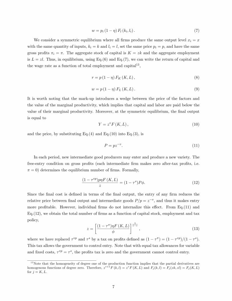
w = pi (1� �)Fl (ki; li) : (7)

We consider a symmetric equilibrium where all �rms produce the same output level xi = x

with the same quantity of inputs, ki = k and li = l; set the same price pi = p; and have the same

gross pro�ts �i = �. The aggregate stock of capital is K = zk and the aggregate employment

is L = zl. Thus, in equilibrium, using Eq.(6) and Eq.(7), we can write the return of capital and

the wage rate as a function of total employment and capital13,

r = p (1� �)FK (K;L) ; (8)

w = p (1� �)FL (K;L) : (9)

It is worth noting that the mark-up introduces a wedge between the price of the factors and

the value of the marginal productivity, which implies that capital and labor are paid below the

value of their marginal productivity. Moreover, at the symmetric equilibrium, the �nal output

is equal to

Y = zvF (K;L) ; (10)

and the price, by substituting Eq.(4) and Eq.(10) into Eq.(3), is

P = pz�v: (11)

In each period, new intermediate good producers may enter and produce a new variety. The

free-entry condition on gross pro�ts (each intermediate �rm makes zero after-tax pro�ts, i.e.

� = 0) determines the equilibrium number of �rms. Formally,

(1� � vp)p�F (K;L)z

= (1� � s)P�: (12)

Since the �nal cost is de�ned in terms of the �nal output, the entry of any �rm reduces the

relative price between �nal output and intermediate goods P=p = z�v; and thus it makes entry

more pro�table. However, individual �rms do not internalize this e¤ect. From Eq.(11) and

Eq.(12), we obtain the total number of �rms as a function of capital stock, employment and tax

policy,

z =

�(1� ��)�F (K;L)

�

� 11�v

; (13)

where we have replaced � vp and � s by a tax on pro�ts de�ned as (1� ��) = (1� � vp)=(1� � s).This tax allows the government to control entry. Note that with equal tax allowances for variable

and �xed costs, � vp = � s; the pro�ts tax is zero and the government cannot control entry.

13Note that the homogeneity of degree one of the production function implies that the partial derivatives arehomogenous functions of degree zero. Therefore, zv+1F (k; l) = zvF (K;L) and Fj(k; l) = Fj(zk; zl) = Fj(K;L)for j = K;L.

7

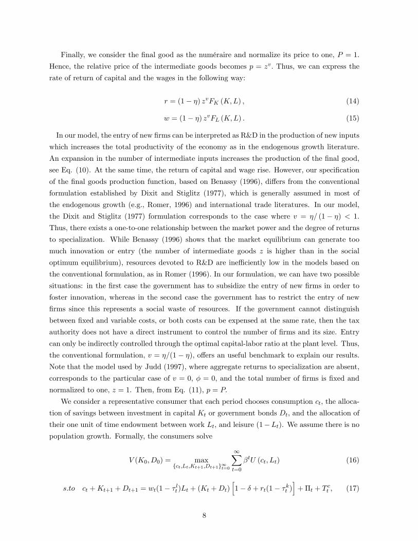
Finally, we consider the �nal good as the numéraire and normalize its price to one, P = 1:

Hence, the relative price of the intermediate goods becomes p = zv: Thus, we can express the

rate of return of capital and the wages in the following way:

r = (1� �) zvFK (K;L) ; (14)

w = (1� �) zvFL (K;L) : (15)

In our model, the entry of new �rms can be interpreted as R&D in the production of new inputs

which increases the total productivity of the economy as in the endogenous growth literature.

An expansion in the number of intermediate inputs increases the production of the �nal good,

see Eq. (10). At the same time, the return of capital and wage rise. However, our speci�cation

of the �nal goods production function, based on Benassy (1996), di¤ers from the conventional

formulation established by Dixit and Stiglitz (1977), which is generally assumed in most of

the endogenous growth (e.g., Romer, 1996) and international trade literatures. In our model,

the Dixit and Stiglitz (1977) formulation corresponds to the case where v = �= (1� �) < 1:

Thus, there exists a one-to-one relationship between the market power and the degree of returns

to specialization. While Benassy (1996) shows that the market equilibrium can generate too

much innovation or entry (the number of intermediate goods z is higher than in the social

optimum equilibrium), resources devoted to R&D are ine¢ ciently low in the models based on

the conventional formulation, as in Romer (1996). In our formulation, we can have two possible

situations: in the �rst case the government has to subsidize the entry of new �rms in order to

foster innovation, whereas in the second case the government has to restrict the entry of new

�rms since this represents a social waste of resources. If the government cannot distinguish

between �xed and variable costs, or both costs can be expensed at the same rate, then the tax

authority does not have a direct instrument to control the number of �rms and its size. Entry

can only be indirectly controlled through the optimal capital-labor ratio at the plant level. Thus,

the conventional formulation, v = �=(1� �); o¤ers an useful benchmark to explain our results.Note that the model used by Judd (1997), where aggregate returns to specialization are absent,

corresponds to the particular case of v = 0, � = 0; and the total number of �rms is �xed and

normalized to one, z = 1. Then, from Eq. (11), p = P:

We consider a representative consumer that each period chooses consumption ct; the alloca-

tion of savings between investment in capital Kt or government bonds Dt; and the allocation of

their one unit of time endowment between work Lt; and leisure (1�Lt). We assume there is nopopulation growth. Formally, the consumers solve

V (K0; D0) = maxfct;Lt;Kt+1;Dt+1g1t=0

1Xt=0

�tU (ct; Lt) (16)

s:to ct +Kt+1 +Dt+1 = wt(1� � lt )Lt + (Kt +Dt)h1� � + rt(1� �kt )

i+�t + T

ct ; (17)

8

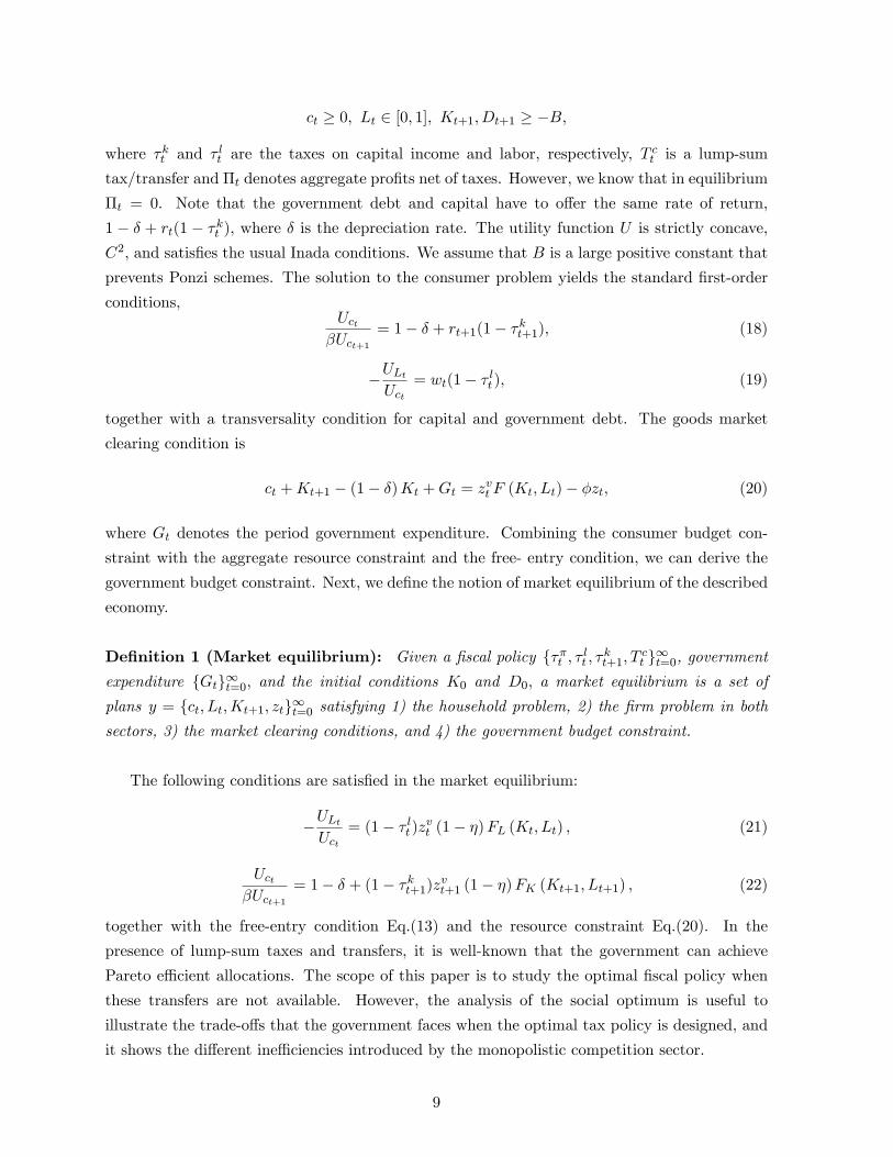
ct � 0; Lt 2 [0; 1]; Kt+1; Dt+1 � �B;

where �kt and �lt are the taxes on capital income and labor, respectively, T

ct is a lump-sum

tax/transfer and �t denotes aggregate pro�ts net of taxes. However, we know that in equilibrium

�t = 0. Note that the government debt and capital have to o¤er the same rate of return,

1 � � + rt(1 � �kt ); where � is the depreciation rate. The utility function U is strictly concave,

C2; and satis�es the usual Inada conditions. We assume that B is a large positive constant that

prevents Ponzi schemes. The solution to the consumer problem yields the standard �rst-order

conditions,Uct�Uct+1

= 1� � + rt+1(1� �kt+1); (18)

�ULtUct

= wt(1� � lt ); (19)

together with a transversality condition for capital and government debt. The goods market

clearing condition is

ct +Kt+1 � (1� �)Kt +Gt = zvt F (Kt; Lt)� �zt; (20)

where Gt denotes the period government expenditure. Combining the consumer budget con-

straint with the aggregate resource constraint and the free- entry condition, we can derive the

government budget constraint. Next, we de�ne the notion of market equilibrium of the described

economy.

De�nition 1 (Market equilibrium): Given a �scal policy f��t ; � lt ; �kt+1; T ct g1t=0, governmentexpenditure fGtg1t=0; and the initial conditions K0 and D0; a market equilibrium is a set of

plans y = fct; Lt;Kt+1; ztg1t=0 satisfying 1) the household problem, 2) the �rm problem in both

sectors, 3) the market clearing conditions, and 4) the government budget constraint.

The following conditions are satis�ed in the market equilibrium:

�ULtUct

= (1� � lt )zvt (1� �)FL (Kt; Lt) ; (21)

Uct�Uct+1

= 1� � + (1� �kt+1)zvt+1 (1� �)FK (Kt+1; Lt+1) ; (22)

together with the free-entry condition Eq.(13) and the resource constraint Eq.(20). In the

presence of lump-sum taxes and transfers, it is well-known that the government can achieve

Pareto e¢ cient allocations. The scope of this paper is to study the optimal �scal policy when

these transfers are not available. However, the analysis of the social optimum is useful to

illustrate the trade-o¤s that the government faces when the optimal tax policy is designed, and

it shows the di¤erent ine¢ ciencies introduced by the monopolistic competition sector.

9

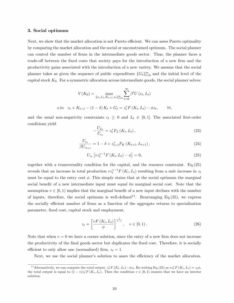
3. Social optimum

Next, we show that the market allocation is not Pareto e¢ cient. We can asses Pareto optimality

by comparing the market allocation and the social or unconstrained optimum. The social planner

can control the number of �rms in the intermediate goods sector. Thus, the planner faces a

trade-o¤ between the �xed costs that society pays for the introduction of a new �rm and the

productivity gains associated with the introduction of a new variety. We assume that the social

planner takes as given the sequence of public expenditure fGtg1t=0 and the initial level of thecapital stockK0. For a symmetric allocation across intermediate goods, the social planner solves:

V (K0) = maxfct;Lt;Kt+1;ztg1t=0

1Xt=0

�tU (ct; Lt)

s:to ct +Kt+1 � (1� �)Kt +Gt = zvt F (Kt; Lt)� �zt; 8t;

and the usual non-negativity constraints ct � 0 and Lt 2 [0; 1]: The associated �rst-order

conditions yield

�ULtUct

= zvt FL (Kt; Lt) ; (23)

Uct�Uct+1

= 1� � + zvt+1FK (Kt+1; Lt+1) ; (24)

Uct�vzv�1t F (Kt; Lt)� �

�= 0; (25)

together with a transversality condition for the capital, and the resource constraint. Eq.(25)

reveals that an increase in total production vzv�1t F (Kt; Lt) resulting from a unit increase in ztmust be equal to the entry cost �: This simply states that at the social optimum the marginal

social bene�t of a new intermediate input must equal its marginal social cost. Note that the

assumption v 2 [0; 1) implies that the marginal bene�t of a new input declines with the numberof inputs, therefore, the social optimum is well-de�ned14. Rearranging Eq.(25), we express

the socially e¢ cient number of �rms as a function of the aggregate returns to specialization

parameter, �xed cost, capital stock and employment,

zt =

�vF (Kt; Lt)

�

� 11�v

; v 2 [0; 1) : (26)

Note that when v = 0 we have a corner solution, since the entry of a new �rm does not increase

the productivity of the �nal goods sector but duplicates the �xed cost. Therefore, it is socially

e¢ cient to only allow one (normalized) �rm, zt = 1.

Next, we use the social planner�s solution to asses the e¢ ciency of the market allocation.

14Alternatively, we can compute the total output, zvt F (Kt; Lt)��zt: Re-writing Eq.(25) as vzvt F (Kt; Lt) = zt�;the total output is equal to (1 � v)zvt F (Kt; Lt) : Then the condition v 2 [0; 1) ensures that we have an interiorsolution.

10

First, we analyze the mark-up or price-marginal cost distortion. Inspection of Eq.(21) and

Eq.(23) reveals that the monopoly power in the intermediate goods sector reduces the wage

below the marginal productivity of labor. The market power introduces a distortion in the

household labor/consumption decision, such that the marginal rate of substitution between

consumption and labor is lower than the marginal productivity of labor. We have the same

distortion in the intertemporal household decision, as Eq.(22) and Eq.(24) show. The marginal

rate of substitution between present and future consumption, Uct=�Uct+1 , is lower than the

intertemporal marginal rate of transformation 1� �+zvt+1FK (Kt+1; Lt+1) : However, this mark-up distortion does not depend on the number of �rms in the market. The social planner can

attain Pareto e¢ cient allocations by implementing

�kt = �lt = ��=(1� �); 8t: (27)

These two subsidies only depend on the mark-up magnitude, and they ensure that the private and

the social returns coincide. Then, and as in Judd (1997), the distortion on capital accumulation

generated by the monopoly power is e¤ectively eliminated.

There exists a second distortion, since the market equilibrium can generate an ine¢ cient

level of �rms. When a �rm has to decide to enter the market it only considers if monopoly

pro�ts are higher than the �xed cost, but it ignores the productivity gains generated by the

introduction of a new intermediate good. Hence, the private bene�ts from entry (monopoly

pro�ts) can be di¤erent from the social bene�ts (productivity increase). In contrast with the

social planner�s choice in Eq.(26), the market allocation for zt in Eq.(13) depends on � instead of

v: The entry of a new �rm in the market is determined by two opposite e¤ects, a complementary

e¤ect and a business-stealing e¤ect. The complementary e¤ect arises from the fact that a new

�rm in the market raises the demand by increasing the productivity in the �nal goods sector.

Then, since pro�ts increase relative to the �xed cost, entry becomes more pro�table. This e¤ect

tends to generate an ine¢ ciently low number of �rms, given that �rms do not take into account

the positive e¤ect of entry on aggregate productivity. The business-stealing e¤ect results from

the fact that the existing �rms in the market have to share the demand with the new �rm,

although this new �rm produces a di¤erentiated product and it does not compete directly with

the incumbent �rms. Therefore, individual pro�ts decline with the number of �rms. This e¤ect

tends to produce excessive entry of �rms, since new �rms enter the market attracted by high

pro�ts but they do not take into account the negative e¤ect on the incumbent �rms. Overall,

the market can generate a number of �rms too low (high) relative to the social optimum when

monopoly pro�ts are too low (high). Therefore, by comparing Eq.(13) and Eq.(26), the Pareto

11

e¢ cient allocation implies setting15,16

��t = (� � v)=�; 8t: (28)

The pro�ts tax can be positive, negative or zero, depending on the relationship between the

mark-up and the returns to specialization. When these returns are strong enough, entry is

insu¢ cient and it is better to subsidize pro�ts, since the increase in the aggregate productivity

due to a new �rm o¤sets the social cost. When the returns to specialization are low enough,

there is excessive entry and a positive pro�ts tax is optimal. Note that the market equilibrium

number of �rms is only e¢ cient when the complementary e¤ect and the business-stealing e¤ect

coincide, v = �:

Two cases deserve special attention. First, in the absence of aggregate returns to special-

ization, v = 0; then ��t = 1 � �=�F (Kt; Lt) : In this case �rms will try to enter the market tocapture monopoly pro�ts, but from a social point of view, the entry of new �rms is a waste of

resources. Therefore, the social planner con�scates all the monopoly pro�ts to prevent entry

of new �rms. Second, in the conventional formulation, v = �= (1� �) ; the market always gen-erates an insu¢ cient number of �rms. Hence the social planner needs to introduce a subsidy

��t = ��=(1 � �), which is identical to the capital and labor subsidies, Eq.(27). However, thisresult could be misleading since the subsidy to entry is not only determined by the mark-up,

since in this case � measures both market power and returns to specialization.

By comparing the social optimum with the market allocation, we clearly identify two market

failures or distortions. First, the mark-up or price-marginal cost distortion implies that capital

and labor are paid below their marginal productivity. Therefore, we have a distortion in both the

household labor/consumption and intertemporal decisions. If lump-sum taxes were available, it

would be possible to eliminate this distortion with the capital and labor subsidies described in

Eq.(27). The second market failure or distortion is the ine¢ cient entry. In the market equi-

librium, the number of �rms is determined by monopoly pro�ts. However, the social optimum

is determined by the productivity growth generated by the introduction of a new intermediate

input. As we can see in Eq.(28), if � > v; the monopoly pro�ts are higher than the social bene�ts

of entry and the social planner introduces a tax on pro�ts in order to avoid a problem of excess

entry. In the opposite case � < v, the market does not generate enough intermediate inputs and

15Clearly, any pairwise f�vpt ; �st g satisfying the condition 1 � ��t = (1 � �vpt )=(1 � �st ) = v=� would be Paretoe¢ cient, as for instance ��t = �

vpt = (�� v)=� and �st = 0; or �vpt = 0 and �st = (v� �)=v: We use the �rst case to

compare the results with other papers.16 In fact, it is not so important that the government can di¤erentiate tax allowances between �xed and variable

costs. As an example, the government could also implement the optimal level of varieties by introducing alump-sum tax/subsidy for the �rm (measured in units of the �nal good) PtT xt . In this case, the optimal tax is

T xt = ���v� 1

�; v > 0;

and ��t = 0 8t: The sign of this instrument also depends on the relation between � and v. Note that when v = 0;then T xt = �F (K;L)� �:

12

the social planner introduces an entry subsidy to increase the productivity of the economy. In

this case, ��t can be interpreted as a subsidy to R&D of new varieties. If the government does

not have access to lump-sum taxes, it needs to take into account these two market failures in

the design of the optimal tax policy.

4. Optimal taxation

In this section, we characterize the optimal �scal policy or constrained optimum. In order to

solve the government problem, we use the primal approach of optimal taxation proposed by

Atkinson and Stiglitz (1980). This approach is based on characterizing the set of allocations

that the government can implement for a given �scal policy. The market equilibrium or set of

implementable allocations is described by the period resource constraints, the equilibrium entry

condition and the so-called implementability constraint. The implementability constraint is the

household�s present value budget constraint after the substitution of the �rst-order conditions of

the consumer�s and �rms�problems. This constraint captures the e¤ect that changes in the tax

policy have on agents decisions and market prices. Thus, the government problem is to maximize

its objective function over the set of implementable allocations. This is called the Ramsey

allocation problem. We present the tax policy as �optimal wedges�rather than a particular tax

system. We can implement optimal allocations as a market equilibrium with distortionary taxes.

In the Appendix, we present the derivation of the implementability constraint and, following

Chari and Kehoe (1999), we show that an implementable allocation can be supported as a

market equilibrium with taxes.

It is well-known that the government has an incentive to heavily tax the initial wealth of

the consumer. This policy amounts to a nondistortionary lump-sum tax. As a result, the

Lagrange multiplier of the implementability constraint would be zero. Given that we already

have characterized the unconstrained optimum, we assume that the initial capital income tax

�k0 is taken as given.

In our framework, the optimal tax policy depends on the government�s ability to di¤erentiate

tax allowances and, hence, to control entry. We consider three di¤erent cases:

� E¤ective control on entry-decisions: the government has a complete set of �scal instru-ments and can directly control entry. This formulation is equivalent to a tax code with

di¤erent tax allowances for �xed and variable cost, or a tax code where �xed cost cannot

be expensed, i.e., � vp 6= � s and the government can introduce a pro�ts tax ��:

� Ine¤ective control on entry-decisions: the government cannot directly choose the numberof �rms. The tax code does not distinguish between variable and �xed costs and, thus,

it is restricted to use the same tax rate, i.e., � vp = � s and the pro�ts tax is not available

�� = 0:

13

� In the third case, suggested by Stiglitz and Dasgupta (1971), we assume that the govern-ment has to apply the same marginal tax to both capital income and pro�ts. In this case,

the government can indirectly control entry through a corporate tax.

4.1. E¤ective control on entry-decisions

Next, we de�ne the government problem for the case where entry-exit decisions are controlled

by the government. This formulation is consistent with a pro�ts tax that di¤erentiates tax al-

lowances between �xed and variable costs, or a tax code where �xed costs cannot be expensed,

i.e. ��t 6= 0. Thus, the tax authority uses the pro�ts tax to control the number of �rms (aggre-gate level of productivity) in the intermediate goods sector. The government will set a subsidy

in case of an insu¢ cient entry or a tax in case of an excessive entry. This case is used as a

benchmark to compare the results with those arising from a limited set of tax instruments.

De�nition 2 (Ramsey allocation problem): Given the government expenditure fGtg1t=0,and the initial conditions f�k0 ;K0; D0g; the allocations associated to the optimal �scal policyf��t ; � lt ; �kt+1g1t=0 are derived by solving

V (K0; D0; �k0 ) = max

fct;Lt;Kt+1;ztg1t=0

1Xt=0

�tU (ct; Lt) ;

s:to

1Xt=0

�t(ctUct + LtULt) = Uc0 (K0 +D0)h1� � + zv0 (1� �)FK (K0; L0) (1� �k0 )

i; (29)

ct +Kt+1 � (1� �)Kt +Gt = zvt F (Kt; Lt)� �zt; 8t;

where ct � 0 and Lt 2 [0; 1]:

Let � and �t be the Lagrange multiplier of the implementability constraint and the resource

constraint, respectively. The �rst-order conditions of the government problem with respect to

fct; Lt;Kt+1; ztg are17

�t [Uct + � (Uct + ctUctct + LtULtct)]� �t = 0; (30)

�t [ULt + � (ULt + LtULtLt + ctUctLt)] + �tzvt FL (Kt; Lt) = 0; (31)

��t + �t+1[1� � + zvt+1FK (Kt+1; Lt+1)] = 0; (32)

17Throughout the paper we assume that the solution of the Ramsey allocation problem exists and converges to aunique steady state. Neither of these assumptions are innocuous. The su¢ cient conditions for an optimum involvethird derivatives of the utility function. Therefore, the solution might not represent a maximum, or the systemmight not have a solution because it does not exist a feasible policy that satis�es the intertemporal governmentbudget constraint. However, if the solution to the government problem exists and is interior, it satis�es the above�rst-order conditions. Hence, the optimal �scal analysis applies only to these cases.

14

vzv�1t F (Kt; Lt)� � = 0; (33)

together with a transversality condition for the capital, the period resource constraint and the

implementability constraint. Note that the Lagrange multiplier � measures the e¤ect of the

distortionary taxes on the utility function, i.e., the burden of taxation or the social cost of tax

revenue. In particular, it can be interpreted as the amount that the households would be willing

to pay in order to replace one unit of distortionary tax revenue by one unit of lump-sum revenue,

measured in terms of the consumption good at time zero.

Comparing Eq.(33) with Eq.(13), we obtain the optimal pro�ts tax

b��t = (� � v)=�: (34)

Note that from now onwards, we use a hat to denote optimality. When the government can

control entry-decisions, it implements a tax/subsidy in the intermediate goods production which

is identical to the social planner tax/subsidy, Eq.(28). As we have seen in Section 3, as long as v >

�; the tax authority subsidizes entry because of the positive e¤ect of the returns to specialization.

However, when v < �; it is optimal to tax pro�ts, since the social cost of introducing a new

�rm o¤sets the productivity gain. Since private �rms do not internalize this e¤ect, the tax

authority has to reduce market entry. Therefore, the government optimally sets the number of

�rms by taking into account only the productivity gains associated with the introduction of a

new variety, regardless of the social cost of tax revenue. This result could be considered as an

application of the Diamond and Mirrlees (1971) principle of aggregate production e¢ ciency18.

The �scal system should allow the economy to be on the production frontier and then individual

decisions among the possible combinations in the frontier are distorted. Diamond and Mirrlees

(1971) show that if the government has a complete set of tax instruments, so that a 100% tax

can be levied on pure pro�ts, the tax system should not distort the allocation of intermediate

inputs. However, as we will see, if the government does not have enough tax instruments to

control entry or to remove the mark-up distortion, this result does not apply and the government

cannot implement the social planner tax/subsidy on entry.

It is straightforward to �nd the long-run optimal capital income tax. From the �rst-order

conditions of the government problem, Eq.(30) and Eq.(32), evaluated in steady state we have

1

�= 1� � + zvFK(K;L): (35)

Comparing this condition with Eq.(22) evaluated in steady state, we obtain the optimal capital

income tax , b�k = ��= (1� �) ; which is the subsidy proposed by Judd (1997, 2002) to remove the18Chari and Kehoe (1999) present a simple derivation of this result. In an economy with two sectors, one

producing the consumption good and the other the intermediate inputs, the tax system should equate marginalrates of transformation across technologies, and the government should not tax intermediate inputs.

15

mark-up distortion on capital accumulation19. As we have seen in the social planner problem, we

need to introduce a capital subsidy to eliminate the wedge between the intertemporal marginal

rate of substitution and transformation. The following proposition summarizes all these �ndings.

Proposition 1: When the government can control entry-decisions:

1) The optimal steady-state capital income tax is negative and it coincides with the social planner

subsidy, as in Judd (1997, 2002). Therefore, it does not depend on the returns to specialization.

2) The optimal pro�ts tax/subsidy coincides with the social planner tax/subsidy. Therefore, it

is always constant and its sign depends on the relationship between the mark-up and the returns

to specialization.

The optimal capital income tax in steady state is negative regardless of the relative magnitude

of the returns to specialization with respect to the mark-up. The government faces a trade-o¤

between the business-stealing e¤ect and the complementary e¤ect, i.e., the �xed cost that society

pays for the introduction of a new �rm and the productivity gains associated to the introduction

of this new variety. Since the government can control the entry of �rms without distorting any

individual or �rm decision, the degree of returns to specialization does not have any impact on

the capital income tax20. Note that both the optimal pro�ts tax and the optimal capital subsidy

coincide with the social planner�s solution. This implies that when the government decides to

subsidize/tax R&D, it ignores the social cost of the labor tax. Besides, the magnitude of the

capital subsidy does not depend on the labor tax distortion. Again, the conventional formulation,

v = �=(1� �); is an interesting case, since the optimal pro�ts tax is equal to the capital subsidyb�� = b�k = ��=(1� �) < 0: This result will later help us to understand the corporate tax.Except for the endogenous entry of �rms, the �rst-order conditions for the government prob-

lem in the economy with imperfectly competitive markets are similar to the conditions for an

economy with competitive markets. As a consequence, we can extend some of the results of the

uniform commodity tax literature to the transition path (see Atkinson and Stiglitz, 1980). An

19Judd (1997) obtains this capital tax in the case of a 100% pro�ts tax. He also presents the case of a �xedpro�ts tax. In this case, the capital subsidy depends on the pro�ts tax and the social cost of taxation. The reasonis that in his model pro�ts are a �pure rent�, hence, a pro�ts tax becomes a lump-sum tax, which helps to reducethe social cost of taxation.20 In fact, it is not so important that the government can di¤erentiate tax allowances between �xed and variable

costs, since the Ramsey allocation can be implemented in several ways. For instance, the intermediate goodssector can be directly controled by the government through a tax �xt on intermediate production x: In this case,the steady-state optimal �scal policy implies

b�x = � � v�

; v > 0;

b�k = [(1� �) v � �] = (1� �) v; v > 0;

and when v = 0 then b�x = 1��=�F (K;L) and b�k = 1��F (K;L)= (1� �)�: In fact, the government uses the taxon the intermediate output to e¢ ciently set the number of varieties, and after it uses the capital income tax toe¢ ciently set the capital-labor ratio by correcting the distortion due to the tax on output, so that (1�b�k)(1�b�x) =1= (1� �) :

16

inspection of the �rst-order conditions gives some insight about the requirements that the utility

function needs to satisfy in order to have constant taxes from t > 1: The proof is in the Appendix.

Corollary 1: For the class of utility functions that are additively separable (across time and

goods) and homothetic with respect to consumption and hours worked, the optimal policy from

t > 1 prescribes constant taxes.

An example of utility function that satis�es this property is

U(ct; Lt) =c1��t

1� � �L1+'t

1 + ': (36)

4.2. Ine¤ective control on entry-decisions

The previous results critically hinge on the assumption that the government has a separate

instrument to control entry. To illustrate this point, we consider the case where the government

sets equal tax allowances for �xed and variable costs. Therefore, the equilibrium number of

�rms or varieties cannot be a¤ected by the �scal authority and production e¢ ciency is not

longer attainable. Thus, ��t = 0 and zt is treated by the government as a variable beyond

its direct control. However, the government knows that it can a¤ect the number of �rms by

changing capital accumulation, but it has to bear a utility cost associated to the change in the

consumption and leisure paths.

Since ��t = 0; the zero pro�t condition without taxes becomes a constraint for an allocation

to be implementable. Combining the free-entry condition Eq.(13) with the resource constraint,

Eq.(20), gives

ct +Kt+1 � (1� �)Kt +Gt = (1� �)F (Kt; Lt)1

1�v

��

�

� v1�v

: (37)

Let � and �t be the Lagrange multiplier associated with the implementability constraint and

the new resource constraint Eq.(37), respectively. Then, the associated �rst-order conditions

with respect to fct; Lt;Kt+1g are

�t fUct + �[Uct + ctUctct + LtULtct ]g � �t = 0; (38)

�t fULt + �[ULt + LtULtLt + ctUctLt ]g+ �t(1� �)(1� v)z

vt FL (Kt; Lt) = 0; (39)

��t + �t+1[1� � +(1� �)(1� v)z

vt+1FK (Kt+1; Lt+1)] = 0: (40)

17

Using Eq.(38) and Eq.(40) evaluated in steady state, we have

1

�= 1� � + (1� �)

(1� v)zvFK(K;L): (41)

Comparing this condition with Eq.(22) evaluated in steady state, we obtain a negative capital

income tax, b�k = �v=(1 � v) < 0; that only depends on the returns to specialization. Given

that v 2 [0; 1) ; the capital income tax is negative. The next proposition summarizes this result.

Proposition 2: When the government cannot control entry-decisions, ��t = 0, then the sign

of the optimal capital income tax in the steady state is negative, regardless of the magnitude

of the mark-up, b�k = �v=(1 � v) < 0 . Nevertheless, in the absence of aggregate returns to

specialization, v = 0; the optimal capital income tax in the steady state is zero.

In contrast with the previous case, the optimal capital income tax does not depend on the

magnitude of the mark-up. Since the government cannot control the �rms�entry, it uses the

capital income tax to partially correct the e¤ects of the returns to specialization. Consequently,

the magnitude of the mark-up does not have any impact on the capital income tax. To explain

the intuition of this result, one particular case deserves special attention. In the absence of

aggregate returns to specialization, v = 0; we should not subsidize capital to eliminate the

mark-up distortion, b�k = 0. In this case, the introduction of a new �rm only has a negative

consequence: a business-stealing e¤ect that translates into a social waste of resources by means

of the �xed cost. As a result, the marginal rate of transformation between present and future

consumption is equal to 1��+(1��)FK(K;L): This means that the return of a unit investmentin terms of future consumption is the marginal productivity of capital FK ; minus the resources

wasted by the �xed cost of new �rms, �FK . The accumulation of capital raises pro�ts by �FK ;

which is used by new �rms entering the market to pay the �xed cost. Since the �xed cost is

a waste of resources, the net increase in future consumption is equal to (1 � �)FK(K;L). Bycomparing Eq.(22) and Eq.(41), in the case of v = 0; we can see that the existence of the mark-up

implies that the return of capital in the market coincides with the optimal return of capital from

the government point of view. Therefore, the government should not subsidize capital to remove

the mark-up distortion. If the government decided to implement the capital subsidy proposed

by Judd (1997), given that the number of �rms cannot be controlled, the capital subsidy would

lead to an ine¢ cient number of �rms. Thus, the threat of entry makes the prescribed capital

income tax to be zero instead of negative. Therefore, in order to implement the Judd (1997)

capital subsidy, the government has to be able to control the number of �rms.

In the more general case, as we can see in equation Eq.(41), there is a complementary e¤ect,

and, then, the entry of new �rms increases the return of investment. Since this externality is

not internalized by the �rms, the government needs to introduce a capital subsidy to promote

entry, b�k = �v=(1 � v): Note that the price-marginal cost distortion is not relevant to design

18

of optimal capital income tax, thus the government should only target the ine¢ cient entry

distortion. However, since the government can only encourage entry through a capital subsidy,

the production e¢ ciency condition should not be implemented, since it would lead to a large

distortion in the capital stock. In particular, in the case of the conventional formulation, v =

�= (1� �) < 1; the optimal capital subsidy is �k = ��=(1 � 2�) < 0: Clearly, this result is a

�mirage�, in the sense that we cannot know if the government should target the price-marginal

cost or the ine¢ cient entry distortion.

This �nding is consistent with some theoretical �ndings in the industrial organization liter-

ature. When the government cannot control the entry decisions on a market and there are no

returns to specialization, a tax or a subsidy leads to a socially ine¢ cient number of �rms, since

it increases the �xed costs; this is called ine¢ cient economies of scale. For instance, Auerbach

and Hines (2002) show that in a static Cournot model with free entry, an output subsidy to

equate the price to the marginal cost encourages ine¢ cient entry of new �rms. Our result proves

to be more general because we are considering a dynamic general equilibrium analysis instead

of a partial equilibrium. Finally, using the same arguments as in the Proof of Corollary 1, it is

straightforward to extend the results of Proposition 2 to the transition path.

4.3. Corporate taxation.

In this section, we consider the case where the government cannot distinguish between capital

income and pro�ts. Therefore, both taxes have to be the same in all periods, �kt = ��t . We call

them corporate taxes, � ct . This tax implies that the government taxes at the same rate all the

income generated by the �rm after paying the labor cost, and the �rm cannot deduct the �xed

cost21. In this tax structure, suggested by Stiglitz and Dasgupta (1971), the government uses

the corporate tax as an indirect way to tax the economic rents or monopoly pro�ts. Judd (1997),

Guo and Lansing (1999) and Schmitt-Grohé and Uribe (2005) consider the optimal corporate

tax in a dynamic model when the number of �rms is �xed. They show that monopoly pro�ts

can yield a positive corporate tax. In our economy, the government uses the corporate tax to

indirectly set the number of �rms zt. We �nd that the optimal corporate tax depends on the

returns to specialization, the mark-up and the curvature degree of the production function. The

assumption that the �rm cannot deduct the �xed cost could be considered unappealing from

the empirical point of view, since the R&D could be considered part of the �xed cost. However,

since the optimal corporate tax does not depend on the �xed cost, the �scal treatment of the

�xed cost is irrelevant to determine the optimal tax. For instance, we could assume that the

government allows to deduct a fraction of the �xed cost, like a R&D allowance, and the outcome

would be the same. The exception occurs when there is a 100% deduction, since we obtain the

tax code of the previous case.

21Note that pF (K;L)�wL = rk+ p�F (K;L): If the government allows the �rm to fully deduct the �xed cost,we have the same tax structure as in the previous case.

19

The tax restriction takes the form of an additional constraint on the Ramsey allocation

problem. In this case, by substituting the tax from Eq.(22) into the zero pro�t condition, we

obtain an additional constraint needed to characterize the set of implementable allocations,�Uct�1�Uct

� 1 + ���

�

�(1� �)

�F (Kt; Lt) = ztFK (Kt; Lt) : (42)

This restriction shows that, from the government�s perspective, the tax distortion due to either

the returns on savings or the introduction of a new �rm has to be the same. In the Appendix

we show that the following steady-state condition is satis�ed:

1

�� 1 + � = zvFK [v + 1� v"� (1� ") (1� � c) �] ; (43)

where " = "FK ;K="F;K = (FKKK=FK) = (FKK=F ) < 0 is the inverse ratio between the elas-

ticities of the production function and of the marginal productivity of capital with respect to

the capital, and it can be interpreted as the curvature degree of the production function. Com-

bining this equation with Eq.(22) evaluated in steady state, we �nd the optimal corporate tax,b� c = [(v � �) "� v] = (1� �") : Note that b� c is bounded above by one. The next Propositionsummarizes this result.

Proposition 3: When the government cannot di¤erentiate between capital income and pro�ts,

then the sign of the optimal steady-state corporate tax is positive whenever v=� < �"=(1 � ")and negative whenever v=� > �"=(1� ").

When pro�ts and capital income taxes cannot be di¤erentiated, the government faces a trade-

o¤ between eliminating distortions associated to the market power and determining the e¢ cient

level of entry. In general, we �nd that the optimal corporate tax can be positive, negative or zero.

It depends on the relative magnitude of the returns to specialization with respect to the mark-up

and the curvature degree of the production function. If the returns to specialization relative to

the mark-up are big enough, then the government lowers the corporate tax in order to promote

the entry of new �rms. The curvature degree of the production function shows how the return

of capital changes with the capital stock. In the absence of returns to specialization, v = 0; then

the optimal corporate tax is positive, in order to prevent the excessive entry of �rms. In the

conventional formulation, v = �=(1��), we obtain that the corporate tax is equal to the capitalsubsidy proposed by Judd (1997, 2002), b� c = ��=(1 � �). As we have seen in the case whenthe government can control entry, capital and pro�ts tax are identical, b�k = b�� = ��=(1 � �).Then, in this case we do not have any con�ict between the price-marginal cost and the inef-

�cient entry distortion. Since we can use the corporate tax to remove the price-marginal cost

distortion in capital accumulation and to achieve the optimal number of �rms, the production

e¢ ciency condition applies to this case. Unfortunately, there is no a prior a reason to believe

20

in this particular combination of parameters. Therefore, we cannot rely on a corporate subsidy

to remove both distortions at the same time. We illustrate this trade-o¤ through the case of a

Cobb-Douglas production function.

Corollary 2: If the production function is F (K;L) = KuL1�u, where u is the production

elasticity with respect to the capital, then "=(1 � ") = (u � 1) and therefore the steady-statecorporate tax is positive if v=� < (1� u) :

4.4. Di¤erentiated consumption and investment goods

We analyze the robustness of the previous results by considering a formulation with di¤erentiated

consumption and investment goods. In particular, we assume that the individual buys several

di¤erentiated consumption goods and derives utility from the following mix:

c =

�zvc(1��)��

Z z

0x1��ci di

� 11��

; � 2 [0; 1) ; vc 2 [0; 1) ; (44)

where xci is the consumption good produced by �rm i; and vc is the degree of returns to

specialization or love of variety for the consumption mix. Investment goods, It, are produced

by competitive �rms through the following technology:

I =

�zvI(1��)��

Z z

0x1��Ii di

� 11��

; � 2 [0; 1) ; vI 2 [0; 1) ; (45)

where xIi is the intermediate good i used to produce investment goods, and vI is the degree of

returns to specialization for the investment. Note that the same varieties are used to consume

and to produce investment goods.

In the Appendix, we show that the social optimum implies the same taxes on labor and

capital income as in the model with one �nal goods sector, but now the steady-state pro�ts tax

is

�� =� (1� vI)� vc (1� �)� (vI � vc)

h��

1��(1��)

i"F;K

� (1� vI + vc): (46)

Since the main forces driving the economy do not change, the social planner allocation does not

change either. Thus, social planner subsidies are determined only by the mark-up, �kt = � lt =

��= (1� �) : Obviously, when vc = vI we recover our previous pro�ts tax, Eq.(28).The socially e¢ cient pro�ts tax depends on the capital depreciation and the elasticity of

the production function with respect to the capital "F;K . Since there exist di¤erent degrees of

returns to specialization, the social planner has to take into account steady-state investment.

However, when depreciation is zero, the optimal tax is

�� =� (1� vI)� vc (1� �)

� (1� vI + vc): (47)

21

Note that sign (@��=@vI) = sign (@��=@vc) < 0; so we have the same e¤ects as when there is

only one �nal goods sector.

We have the same qualitative results and e¤ects in the optimal tax policy. In particular,

when the government can control entry, ��t 6= 0, we obtain in steady state that the optimal pro�tsand capital income tax are equal to the socially e¢ cient values. Besides, when the government

cannot control entry ��t = 0, the optimal capital subsidy is equal to

b�k = �� (vc � vI) "F;K � vc [1� � (1� �)]�� (vc � vI) "F;K + (1� vI) [1� � (1� �)]

: (48)

Again, given that the government cannot control entry, the capital subsidy should not be used

to eliminate the mark-up distortion, but it should be used to encourage entry. The corporate

tax, in the case of no depreciation � = 0; is (the general case is in the Appendix)

b� c = (vI � vc) � + [��"+ (vc � vI) � (1� ")� vc (1� ")](1 + vc � vI) (1� �")

: (49)

Note that when vc = vI ; the tax policy coincides with the one �nal goods sector model. Hence,

we can conclude that the introduction of di¤erentiated consumption and investment goods does

not change the qualitative results of the paper, but it can a¤ect the optimal magnitude.

5. Conclusions

In recent papers, Judd (1997, 2002) has presented evidence in favor of a negative capital income

tax. Using a representative-agent model with a �xed number of goods produced by monopolistic

�rms, he �nds that the optimal �scal policy implies a negative capital income tax and a 100%

tax rate on �rms�pro�ts.

The main contribution of our paper is to show that once we consider an endogenous number

of �rms or varieties, the optimal �scal policy can lead to di¤erent results. We show that the

optimal �scal policy is conditioned by the existence of two market failures: market power and

ine¢ cient entry. In particular, the capital income tax depends on the government�s ability to

control entry through a tax on variable pro�ts. We follow the formulation of Ethier (1982)

and Benassy (1996) to separate the mark-up from the index of returns to specialization, which

measures the trade-o¤ between the �xed costs that society pays for the introduction of a new

�rm and the productivity gains associated to this new �rm.

We consider three di¤erent cases. In the �rst case, we assume that the government can

levy a tax on pro�ts, so that the government can control entry. The government implements a

capital subsidy to remove the price-marginal cost distortion on capital accumulation, as in Judd

(1997, 2002). Besides, the optimal pro�ts tax coincides with the tax that a social planner would

implement if lump-sum taxes were available. We show that both the capital subsidy and the

pro�ts tax do not depend on the tax burden. One important implication of these results is that

22

if the government has available a complete set of taxes, the subsidies to promote the entry of

new �rms or R&D should not be constrained by the tax burden.

In the second case, we assume that the government cannot tax pro�ts, so the equilibrium

number of �rms cannot be directly controlled by the �scal authority. With this tax code re-

striction, we �nd that the government should not implement a capital subsidy to remove the

price-marginal cost distortion, but that the capital subsidy should be used to encourage the

entry of �rms, then it does depend on the returns to specialization. In contrast with Judd

(1997, 2002), we show that in the absence of aggregate returns to specialization the optimal

steady-state capital income tax is zero.

In the third case, suggested by Stiglitz and Dasgupta (1971), the government has to apply the

same marginal tax to both capital income and pro�ts. In this case the government can indirectly

control entry through a corporate tax. We �nd that the optimal corporate tax depends not only

on the magnitude of the returns to specialization and the mark-up, but also on the curvature

degree of the production function. Also, we show that the results remain unchanged if we

consider di¤erentiated consumption and investment goods.

Finally, our results highlight the idea that the optimal tax system would depend on the

information available about the structure of the economy: market power, productivity of the

R&D, etc. Since this information could be considered as �rms� private information, future

research could consider the introduction of informational or enforcement constraints, following

the Mirrlees�s (1971) approach. Recently, Golosov, Kocherlakota and Tsyvinski (2003) have

developed the Mirrlees approach in a dynamic setting. Their work could be extended to analyze

the issues considered in this paper.

23

Appendix

Derivation of the implementability constraint: The implementability constraint can be

derived as follows. Multiplying Eq.(19) by Lt we have

�LtULt = Uctwt(1� � lt )Lt: (A.1)

Multiplying Eq.(17) by Uct and using Eq.(A.1) gives

ctUct + LtULt = (Kt +Dt)Uct

h1� � + rt(1� �kt )

i� (Kt+1 +Dt+1)Uct : (A.2)

Multiplying Eq.(A.2) by �t and adding up from t = 0 to t =1 yields

1Xt=0

�t (ctUct + LtULt) = (K0 +D0)Uc0

h1� � + r0(1� �k0 )

i

+

1Xt=0

�t��(Kt+1 +Dt+1)Uct+1

h1� � + rt+1(1� �kt+1)

i� (Kt+1 +Dt+1)Uct

�: (A.3)

Using Eq.(A.3), Eq.(8) and Eq.(18) we obtain the implementability constraint, Eq.(29).

Equivalence between an implementable and a market allocation: An allocation in the

market equilibrium y = fct; Lt;Kt+1; ztg1t=0 satis�es the set of implementable allocations. More-over, if an allocation y is implementable, then we can construct a tax policy f��t ; � lt ; �kt+1g1t=0and prices frt; pt; wtg1t=0; such that the allocation together with prices and the policy constitutea market equilibrium.

Proof: The �rst part of the claim is always satis�ed, since any market equilibrium allocation has

to satisfy the resource constraint, the zero pro�t condition and the implementability constraint.

Now we prove the second part of the claim. Given an implementable allocation y, the market

prices can be backed out using Eq.(8), Eq.(9) and Eq.(11). The tax policy is recovered from

Eq.(13), Eq.(18) and Eq.(19). Substituting Uct and ULt in the implementability constraint we

obtain the consumer budget constraints, from where we recover the level of debt. If the resource

constraint and the consumers budget constraints are satis�ed, then the government budget con-

straint is also satis�ed.

Proof of Corollary 1: The class of utility functions that are additively separable (across time

and goods) and homothetic with respect to consumption and hours worked satisfy

LtULtLt + ctUctLt = DULt ; (A.4)

24

ctUctct + LtULtct = EUct ; (A.5)

where D and E are di¤erent constants, and separability between consumption and hours worked

implies UctLt = ULtct = 0: In this case, the �rst-order conditions of the government problem can

be written asUct�Uct+1

= 1� � + zvt+1FK (Kt+1; Lt+1) ; (A.6)

� [1 + �(1 +D)]ULt[1 + �(1 + E)]Uct

= zvt FL (Kt; Lt) ; (A.7)

where � is constant. Clearly, from the market equilibrium Eq.(22), we derive the optimal capital

income tax b�kt+1 = � �

(1� �) : (A.8)

From the consumption-labor decisions Eq.(21), we can derive the optimal labor tax

1� b� lt = [1 + �(1 + E)]

[1 + �(1 +D)]

1

(1� �) : (A.9)

For the example stated in Eq.(36), we have E = �� and D = ', and clearly E < D: Note that

�; and therefore b� lt , depends on the initial conditions K0 and D0. Both taxes are constant fort > 1. At t = 1; the �rst-order conditions contain additional terms.

Derivation of the optimal corporate tax Eq.(43): Substituting Eq.(42) into the aggregate

resource constraint, we obtain a new resource constraint,

ct +Kt+1 � (1� �)Kt +Gt =24�Uct�1�Uct

� 1 + ���

� (1� �)FK (Kt; Lt)

35v F (Kt; Lt)v+1 ��Uct�1�Uct

� 1 + ���F (Kt; Lt)

(1� �)FK (Kt; Lt): (A.10)

Let � and �t be the Lagrange multiplier of the implementability constraint and the new resource

constraint, respectively. The �rst-order conditions of the government problem with respect to

fct; Lt;Kt+1g; after substituting for Eq.(42), are

�t [Uct + � (Uct + ctUctct + LtULtct)]� �t

0@1 +24 Uct�1Uctct

�U2ct

�Uct�1�Uct

� 1 + ��35 [vzvt F (Kt; Lt)� zt�]

1A

+�t+1

24 Uctct

�Uct+1

�Uct

�Uct+1� 1 + �

�35 �vzvt+1F (Kt+1; Lt+1)� zt+1�� = 0; (A.11)

25

�t [ULt + � (ULt + LtULtLt + ctUctLt)] + �tzvt

�(v + 1)FL (Kt; Lt)� v

F (Kt; Lt)FKL (Kt; Lt)

FK (Kt; Lt)

���tzt�

�FL (Kt; Lt)

F (Kt; Lt)� FKL (Kt; Lt)FK (Kt; Lt)

�� �t

Uct�1UctLt

�U2ct

�Uct�1�Uct

� 1 + �� [vzvt F (Kt; Lt)� zt�]

+�t+1

24 UctLt

�Uct+1

�Uct

�Uct+1� 1 + �

�35 �vzvt+1F (Kt+1; Lt+1)� zt+1�� = 0; (A.12)

��t + �t+1�1� � +

�zvt+1FK (Kt+1; Lt+1)

� v + 1 +

�F (Kt+1; Lt+1)FKK (Kt+1; Lt+1)

FK (Kt+1; Lt+1)FK (Kt+1; Lt+1)

�"z1�vt+1 �

F (Kt+1; Lt+1)� v#�

z1�vt+1 �

F (Kt+1; Lt+1)

!)= 0:

(A.13)

Substituting �t+1 from Eq.(A.11) into Eq.(A.12), evaluating the resulting equation in steady

state and dividing it by the same equation one period forward, we obtain that

��t = �t+1: (A.14)

Noting that " = "FK ;K="F;K = (FKKK=FK) = (FKK=F ) < 0 and using Eq.(13) and Eq.(A.14),

in steady state Eq.(A.13) becomes Eq.(43).

Di¤erentiated consumption and investment goods: Next, we consider the market equi-

librium. The inverse demand function for each consumption good and intermediate good used

to produce investment goods is

xji =

�piPj

�� 1�

zvj

(1��)�

�1j; j = c; I; (A.15)

where Pj is the price of good j22. Each goods �rm solves

maxfki;lig

�i = (1� ��) [pi (xci + xIi)� rki � wli]� PI�; (A.16)

subject to the demands, Eq.(A.15), and the production function. The prices at the symmetric

equilibrium are

Pj = z�vjp; j = c; I: (A.17)

We normalize the price of intermediate inputs, p = 1. The �rst-order conditions of the monop-

olistic �rm combined with Eq.(A.17) show that we have a mark-up distortion. Moreover, the

22Pj is an index associated to the composite good, Pj = z�vj+�=(1��)�R z

0p(��1)=�i di

��=(��1); j = c; I:

26

entry of �rms increases the return of capital r=PI and the purchasing power of wages w=Pc,

r

PI= zvI (1� �)FK (K;L) ; (A.18)

w

Pc= zvc (1� �)FL (K;L) : (A.19)

The free-entry condition indicates that the number of �rms depends on vI ; since the �xed cost

is de�ned in terms of the investment good,

z =

�(1� ��)�F (K;L)

�

� 11�vI

: (A.20)

The individual budget constraint is

Pctct + PIt(Kt+1 � (1� �)Kt) +Dt+1 = wt(1� � lt )Lt +RtDt +Ktrt(1� �kt ) + �t + T ct ; (A.21)

whereRt is retrun of government debt. Maximizing Eq.(16) subject to Eq.(A.21) yields

�ULtUct

=wt(1� � lt )

Pct; (A.22)

Uct�Uct+1

=PctPct+1

PIt+1PIt

�1� � + rt+1

PIt+1(1� �kt+1)

�: (A.23)

The equilibrium condition in the output markets is

z�vct (ct +Gt) + z�vIt [Kt+1 � (1� �)Kt] = F (Kt; Lt)�

�z�vIt �

�zt: (A.25)

The social planner maximizes Eq.(16) subject to Eq.(A.25). From the �rst-order conditions with

respect to ct; Lt and Kt+1; we have

�ULtUct

= zvct FLt ; (A.26)

Uct�Uct+1

=zvct+1zvct

zvItzvIt+1

�1� � + zvIt+1FKt+1

�: (A.27)

Combining these last two equations with those of the market equilibrium, we derive the same

steady-state labor and capital income taxes as when there is only one �nal goods sector. The

�rst-order condition with respect to zt is

�vcz�vc�1t (ct +Gt)� vIz�vI�1t [Kt+1 � (1� �)Kt] + (1� vI) z�vIt � = 0: (A.28)

Substituting Gt and � from Eq.(A.25) and Eq.(A.20), respectively, into Eq.(A.28), and evaluat-

27

ing the resulting equation in steady state, we obtain that

(1� vI + vc) (1� ��)� = vc + (vI � vc) �z�vIK

F: (A.29)

Multiplying Eq.(A.27) by Kt+1; and evaluating it in steady state, we have

z�vIK =FKK

1� � 1 + �

: (A.30)

Combining the last two equations gives Eq.(46).

For the tax policy, the implementability constraint is

1Xt=0

�t(ctUct + LtULt) = Uc0

h1� � + zvI0 (1� �)FK (K0; L0) (1� �k0 )

i PI0Pc0

(K0 +D0) : (A.31)

Repeating the same process of the paper, we obtain Eq(48) and the following corporate tax:

b� c = (vI � vc) [� (1� �) + �� ("FK ;K � "F;K) (1� �)] + [1� � (1� �)] [(1 + vc � vI) � (1� ")� � � vc (1� ")](1� �) (1� � (1� �) + (vc � vI) [1� � � �� ("FK ;K � "F;K)]) + [1� � (1� �)] (1 + vc � vI) � (1� ")

:

(A.32)

In the case � = 0; we obtain Eq.(49).

28

References

Atkinson, A.B. and J. Stiglitz, 1980, Lectures on Public Economics, McGraw-Hill, New York.

Auerbach, A.J. and J.R. Hines, 2002, Taxation and Economic E¢ ciency, in: A.J. Auerbach

and M Feldstein, eds., Handbook of Public Economics, vol. 3, North-Holland, Amsterdam,

1347-1421.

Benassy, J.P., 1996, Taste for Variety and Optimum Production Patterns in Monopolistic

Competition, Economics Letters 52, 41-47.

Benassy, J.P., 1998, Is There Always Too Little Research in Endogenous Growth with Expand-

ing Product Variety?, European Economic Review 42, 61�69.

Blanchard, J. and N. Kiyotaki, 1987, Monopolistic Competition and the E¤ects of Aggregate

Demand, American Economic Review 77, 647-666.

Chamley, C., 1986, Optimal Taxation of Capital Income in General Equilibrium with In�nite

Lives, Econometrica 54, 607-622.

Chari, V.V. and P.J. Kehoe, 1999, Optimal Fiscal and Monetary Policy, in: J.B. Taylor and

M. Woodford, eds., Handbook of Macroeconomics, vol. Ic, North-Holland, Amsterdam,

1671-1745.

de Groot, H.L.F. and R. Nahuis, 1998, Taste for Diversity and the Optimality of Economic

Growth, Economics Letters 58, 291�295.

Diamond, P.A. and J.A. Mirrlees, 1971, Optimal Taxation and Public Production: I�Production

E¢ ciency, American Economic Review 61, 8-27.

Dixit, A.K. and J.E. Stiglitz, 1977, Monopolistic Competition and Optimum Product Diversity,

American Economic Review 67, 297-308.

Ethier, W.J., 1982, National and International Returns to Scale in the Modern Theory of

International Trade, American Economic Review 72, 389-405.

Golosov, M., Kocherlakota, N. and A. Tsyvinski, 2003, Optimal Indirect and Capital Taxation,

Review of Economic Studies 70, 569-587.

Guo, J.T. and K.J. Lansing, 1999, Optimal Taxation of Capital Income with Imperfectly Com-

petitive Product Markets, Journal of Economic Dynamics and Control 23, 967-695.

Jones, C.I. and J.C. Williams, 2000, Too Much of a Good Thing? The Economics of Investment

in R&D, Journal of Economic Growth 5, 65�85.

29

Judd, K.L., 1985, Redistributive Taxation in a Simple Perfect Foresight Model, Journal of

Public Economics 28, 59-83.

Judd, K.L., 1997, The Optimal Tax Rate for Capital Income is Negative, NBERWorking Paper

6004.

Judd, K.L., 2002, Capital-Income Taxation with Imperfect Competition, American Economic

Review 92, 417-421.

Kim, J., 2004, What Determines Aggregate Returns to Scale?, Journal of Economic Dynamics

and Control 28, 1577-1594.

Mankiw, N.G and M. Weinzierl, 2004, Dynamic Scoring: A Back-of-the-Envelope Guide,

mimeo.

Matsuyama, K., 1995, Complementarities and Cumulative Processes in Models of Monopolistic

Competition, Journal of Economic Literature 33, 701-729.

McGrattan, E.R. and E.C. Prescott, 2000, Is the Stock Market Overvalued?, Federal Reserve

Bank of Minneapolis Quartely Review 24 (4), 20-40.

Mirrlees, J., 1971, An Exploration in the Theory of Optimum Income Taxation, Review of

Economic Studies 38, 175-208

Romer P.M, 1986, Increasing Returns and Long Run Growth, Journal of Political Economy

94, 1002-1037.

Rotemberg, J. and M. Woodford, 1995, Dynamic General Equilibrium Models with Imperfectly

Competitive Product Markets, in: F.T. Cooley, ed., Frontier of Business Cycles Research,

Princeton University Press, 243-293.

Schmitt-Grohé, S., 1997, Comparing Four Models of Aggregate Fluctuations due to Self-

Ful�lling Expectations, Journal of Economic Theory 72, 96-147.

Schmitt-Grohé, S. and M. Uribe, 2004, Optimal Fiscal and Monetary Policy under Imperfect

Competition, Journal of Macroeconomics 26, 183-209.

Schmitt-Grohé, S. and M. Uribe, 2005, Optimal Fiscal and Monetary Policy in a Medium-

Scale Macroeconomic Model, in: M. Gertler and K. Rogo¤, eds., NBER Macroeconomics

Annual, vol. 20, MIT Press, 383-425.

Stiglitz, J. and P. Dasgupta, 1971, Di¤erential Taxation, Public Goods, and Economy E¢ -

ciency, Review of Economics Studies 38, 655-677.

Wu, Y. and J. Zhang, 2000, Endogenous Markups and the E¤ects of Income Taxation: Theory

and Evidence from OECD Countries, Journal of Public Economics 77, 383-406.

30