UNIVERSITY OFILLINOIS LIBRARY

AT URBANA-CHAMPAIGNBOOKSTACKS

Digitized by the Internet Archive

in 2011 with funding from

University of Illinois Urbana-Champaign

http://www.archive.org/details/equilibriumimper1039kols

)OPY 2

STX

--"is?

i\*T. TV I

FACULTY WORKINGPAPER NO. 1039

Equilibrium, Imperfect Competition and

the Internationa! Wheat Market

Charles D. Kolsiad

Anthony E. Burris

THE LIBRARY Of; JEFIB

fj 1984JUL

V OF ILLINOISHAMPAIQN

College of Commerce and Business Administration

Bureau of Economic and Business ResearchUniversity of Illinois. Urbana-Chamoaign

BEBRFACULTY WORKING PAPER NO. 1039

College of Commerce and Business Administration

University of Illinois at Urbana-Champaign

April, 1984

Equilibrium, Imperfect Competition andthe International Wheat Market

Charles D. Kolstad, Assistant ProfessorDepartment of Economics

Anthony E. Burr isLos Alamos National Laboratory

EQUILIBRIUM, IMPERFECT COMPETITION ANDTHE INTERNATIONAL WHEAT MARKET

by

Charles D. Kolstad and Anthony E. Burris

ABSTRACT

The simple model of perfect competition in

spatial markets has been widely applied in ana-lyzing international agricultural trade. Yet manymarkets do not appear to be perfectly competitive.In this paper we offer a new and efficient methodfor computing spatial equilibrium in oligopolisticor oligopsonistic markets. We apply the techniqueto an analysis of several hypotheses of marketconduct in the international wheat market that havebeen put forward by other authors. We conclude that

a duopsony model with Cournot-Nash behavior (styledafter Carter and Schmitz) does not perform well in

explaining trade.

-2-

I. INTRODUCTION

The simple model of perfect competition in spatial markets has

been widely applied in analyzing international agricultural trade.

Following the developments of Samuelson and Takayama and Judge, it is

relatively easy to formulate and solve detailed and complex spatial

competitive equilibrium models. Yet as Thompson points out, analyses

based on the simple competitive model have yielded disappointing

results. Simple competitive theory seems unable to explain trade in

many agricultural markets.

It is often suggested that the poor performance of the simple com-

2petitive model is due to the interference of governments in markets

or to manipulation by other market participants such as trading com-

panies (Webb, McCalla and Josling, and Morgan). Nearly 20 years ago

McCalla proposed that a US-Canada duopoly (with market power exercised

through government policy) was the more appropriate market conduct

assumption for the international wheat market. Later, Alaouze et al

and Carter and Schmitz suggested a triopoly and a duopsony, respectively,

as more appropriate market structure and conduct assumptions in this

market. Yet such imperfect competition hypotheses have made negligible

3inroads into applied trade analysis.

The purpose of this paper is to bridge this gap between the

apparent structure and conduct of the international wheat market and

quantitative analyses of market performance. In doing so, we present

a new and efficient method for computing spatial equilbria in oligopo-

listic markets. The model and solution technique are based on non-

linear complementarity and represent a very promising way of formulating

-3-

and solving both competitive and noncompetitive spatial equilibrium

problems. We then test various hypotheses of market conduct (mentioned

above) in the international wheat market using a simple imperfectly

competitive wheat trade model. Because of the methodological focus of

this paper, we have chosen to utilize costs and demands from Shei and

Thompson's previously published and relatively small model of the inter-

national wheat market. Thus, in essence we use their model, modifying

only their assumptions about market conduct and their computational

technique for finding market equilibria.

In the next section we review relevant developments in agri-

cultural trade analysis. In the third section of the paper we present

our model of reaction function equilibria and in the fourth section we

apply the model to the international wheat market as we attempt to

accept or reject several hypotheses about conduct in that market.

II. AGRICULTURAL TRADE MODELS

As in most economic analysis the paradigm of perfect competition

4is widely used in evaluating agricultural trade and trade policies.

In his thorough review of US developments in agricultural trade

models, Thompson states that spatial price equilibrium models are

"the most common class of agricultural trade models, particularly for

comparative statics analysis of the effects of a change in policy."

Thompson supports this statement by citing nearly three dozen spatial

equilibrium models of international markets for wheat, rice, corn,

sugar, pork, beef, oranges, rapeseed, and peanuts.

Despite its popularity, it has been recognized for some time that

the paradigm of simple spatial competitive equilibrium suffers from

significant deficiencies, most notably poor performance in explaining

-4-

trade patterns, particularly for wheat. Characteristically, such

models predict fewer bilateral trades than actually occur, although

many actual transactions are quite small. This class of models also

exhibits a high degree of sensitivity of equilibrium trade levels to

small parameter changes. In essense, the simple model of spatial per-

fect competition does not seem consistent with how international agri-

cultural markets operate.

There have been a number of different attempts to correct these

problems. One approach has been to hypothesize that commodities from

different suppliers are not perfect substitutes, despite their physi-

cal similarities. This differentiation may be due to institutional

factors, historic trade preferences or attitudes toward risk. The

result is that demand becomes more complex than in the simple com-

petitive model. This type of demand system is best exemplified by the

work of Armington.

A major thrust of the literature in correcting the predictive

deficiency of spatial equilibrium models is to examine more closely

the role of governments in markets. If one accepts that government

policy is predominantly responsible for differences between actual

trade patterns and those predicted by the simple competitive model,

then the focus of the analysis should be upon the determinants of

government policy.

"Endogenizing" government policy in trade analysis has taken two

directions. One direction has been to assume that government policy

is determined by domestic political factors and not by market power

considerations. The focus of such work is on governmental objectives

-5-

in the policy-setting process (see Rausser et al). Sarris and

Freebairn examine the international wheat market and estimate the

relative weights governments place on domestic producer surplus, con-

sumer surplus, support program costs, and price stability. In an ana-

lysis of the soybean/rapeseed market, Meilke and Griffith estimate

government behavioral equations for the setting of tariffs and

domestic price supports for these commodities.

A second approach to analysis with endogenous government policy is

to assume that policies serve to coordinate consumers or producers so

that they may jointly exercise power in the international market.

Thus the international market would be expected to operate as any

oligopoly/oligopsony with countries as the participants. In 1966,

McCalla suggested that two producing countries dominate the world

wheat market and produce and price accordingly. Later Alaouze et al

proposed expanding the list of oligopolists to three by adding

Australia. Carter and Schmitz suggested that an EEC-Japan duopsony is

responsible for observed wheat trade and price patterns. On the

empirical side, Jeon has developed a non-spatial dynamic model of

duopoly in the world wheat market and Karp and McCalla have modeled

o

the world corn market as a difference game.

A simpler form of market manipulation is through the cartelization

of producers (or consumers). Schmitz et al have analyzed in depth the

possibility of a grain exporter's cartel. Pindyck has estimated the

potential gains from cartelization in the bauxite, copper and petroleum

markets while Pincus and Johnson have analyzed the potential cartel

profits for a number of agricultural commodities.

-6-

III. SPATIAL EQUILIBRIA IN IMPERFECTLY COMPETITIVE MARKETS

The purpose of this paper is to explore the hypothesis that the

international wheat market is imperfectly competitive. We propose to

test this hypothesis by introducing a spatial model of imperfect com-

petition in that market. However, one must be careful in defining a

model of imperfect competition. On the face of it, there are far too

many individual producers and consumers to apply any conventional model

of imperfect competition to the wheat market. However, if producers

(or consumers) are organized into a small number of groups and within

a group all producer (or consumer) actions are coordinated, then we

have an oligopoly (or oligopsony) among a few cartels of producers (or

consumers). In this paper the natural grouping is the nation (or, for

the EEC, several nations). Governments serve as coordinators of produ-

cers and consumers, looking after their interests as groups. The model

then is of imperfect competition among nations. A few nations dominate

the market from either the producing or consuming side and set tariffs,

price supports, quotas or other instruments to maximize the economic

welfare of the producers of consumers they represent.

With that introduction we will move to describe our model of

imperfect competition. Although the actors in the model are pro-

ducing and consuming nations , without loss of generality the model is

described mathematically in terras of a few producers and consumers

interacting in an imperfectly competitive market. To enhance the

model description, we will present it in two steps. We first discuss

reaction function models and present a simple model of spaceless

-7-

reaction function equilibria. We then present a model of spatial oli-

gopoly and oligopsony.

To understand why the model is presented in the particular form it

is, the reader should be aware that the model is formulated and solved

9as a nonlinear complementarity problem. Let there be some n x 1 vector

of variables, _x_, and an n x 1 vector valued function, f(x) . The nonli-

near complementarity problem is to find an _x__>__0_ so that f(x) _>_ 0_ and

x.f.(x) = for all i. In other words we seek a vector x with non-i l — —

negative components so that £XjO is also nonnegative. Further,

matching _x with _f_(_x) , component by component, at least one member of

each pair of x. and f.(x) must be zero. As will become evidentl l

—

throughout the remainder of this section, the models of imperfect com-

petition presented here are precisely of this form. Efficient computer

algorithms are available for solving the linear and nonlinear compli-

10mentarity problem.

A. A Spaceless Reaction Function Oligopoly Model

Consider the case of I producers of a single commodity. Denote by

q. the output of the ith producer and denote by tt. (_q_) the profit of

the ith producer. (Tt is not necessary to explicitly consider demand

since each producer's profit function involves the output of all

producers). Each producer (i) has the simple problem of choosing q.

to maximize tt. :

l

max tt. (_q_)

(la)

q,-

q. > (lb)1

-8-

If ii is pseudoconvex then necessary and sufficient conditions for

profit maximization are:

dir.

+ X* =dq,

(2a)

X*q. =

A*,q. >

(2b)

(2c)

or equivalently,

dir.

<dq." (3a)

dir,

dq.

*q. >

= 0. (3b)

(3c)

Note two things about equation (3). First, it is in the form of a

nonlinear complementarity problem, and secondly, the two equations im-

plicitly define the optimal output for producer i as a function of the

output of all other producers: q.(q.., ..., q._-,> q- + i» •••> q )•

This of course is producer i's reaction function or best reply func-

tion (see Friedman). The reaction function model can take on many

forms depending on how the producer thinks his profits will change as

he changes output (dfr./dq.). It is in computing the derivative of

profit with respect to output that conjectures about behavior of com-

petitors enter. It is conventional to express such conjectures

through a "conjectural variation." Let r. . be the conjectural

-9-

variation of producer i with respect to producer j; i.e., r. . is pro-

ducer i's conjecture of how q. will change when q. is changed3q

i

'

(r. .= ,

J, conjectured). Thus Eqn. (3) can be rewritten as

3tt.

I -r-i- r. . : (4a)tfq . ii —

J 3

qi

3tt.

£ -5— r. .= (4b)

q. > (4c)

where of course r. . = 1. A Nash equilibrium in this market can beii

determined by finding a vector _q_* which satisfies a pair of Eqn. 4 for

each producer (I inequalities, I equalities).

The various models of reaction function equilibrium differ in the

assumed conjectural variation. A Cournot-Nash equilibrium corresponds

to r. .= 0, i * j and can be thought of as a maximum market power non-

cooperative equilibrium in that each producer behaves as if he were

a single monopolist facing a residual demand curve. He takes no

account of the response of competitors to his actions. On the other

hand, a Bertrand equilibrium corresponding to 2 r., = -1, is a mini-k*i

mum market power situation. In this case, each producer assumes that

any reduction in his own output will be exactly matched by competitors.

In the case when outputs from different producers are perfect substi-

tutes, the Bertrand model results in marginal cost pricing.

B. Spatial Oligopoly/Oligopsony With A Competitive Fringe

We now extend our model to a spatial market. The model presented

here is of a spatial market for a single good at a point in time. The

-10-

essence of the spatial aspects of the market is that transportation of

goods from producers to consumers is a costly process. While the model

is presented in terms of producers and consumers, it is producer and

consumer nations (or groups of nations) that will be assumed to exer-

cise market power when the model is applied to the international wheat

market. We present two different but similar spatial models, one of

oligopoly and one of oligopsony.

Let 1=1, ..., 1 index producers and j = 1, ..., J index con-

sumers, and further, let

q.. denote quantity shipped from producer i to consumer j

T. . denote the unit transport cost from producer i to con-

sumer j

P.(Zq..) denote the inverse demand function for consumer i

J . lj

c .( Eq . . ) denote the marginal cost function for producer i.

l .11 r

J

The first of these variables is endogeneous, to be computed. The

transport cost and the marginal cost and inverse demand functions are

exogenous. Note that by indexing the shipments by origin and destina-

tion, we are allowing producers or consumers to price discriminate.

Producers and consumers that are price takers will price at marginal

cost or along their demand curve, in equilibrium. Producers exer-

cising market power will price at or above marginal cost. Consumers

exercising market power will offer prices at or below their demand

curve. Although market-manipulating producers and consumers can both

be included in a single model, for clarity of exposition we will treat

these two situations separately.

-Il-

ia A Model of Spatial Oligopoly

We first consider a model of oligopoly, with some nation-producers

exercising market power and all others in a competitive fringe. All

consumers can be totally represented by their inverse demand curves.

Thus there are two types of producers in the market: oligopolists and

the competitive fringe. Denote the set of oligopolists by M = {i|i is

an oligopolist}. Each producer has the same objective, to maximize

profits over q.. > 0:ij —

£q. .

J1J

it. = E (P.(Z q.,.) - T..) q.. - / c.(x)dx . (5)

The price the producer faces is the consumer price (P.) less the

transport cost (x..). Thus the first term in Eqn. 5 represents reve-ij

nues. The second term, the integral under the marginal cost curve,

represents total variable costs. Producers maximize profits by

choosing quantity sold to each consumer, q... As in equation (3), the

12first order conditions for a maximum of (5) are

(6)

dP.

w.. = [P,(Z q.,.) - T.. + q.. - 2-- c.(Z q. .,)} < 0, q. . > 0, w. .q. .= 0,Vj

ij J if i J iJ ij dqt

i jt ij — iJ — ij ij

In the expression above, the dummy variable w. . is used to facili-

tate indicating that the term in braces must be nonpositive and that

its product with q.., must be zero. The complementarity condition is

necessary because we would expect some flows (q..) to be zero and thus

the corresponding w. . to be perhaps negative. The first three terras

of the expression in braces of course represent marginal revenue. A

fundamental distinguishing characteristic of a spatial model of trade

is that one cannot determine a priori which producer-consumer pairs

-12-

will have no trade (q.. = 0). Thus the necessity for this condition

which is more complex than just marginal revenue equals marginal cost.

For a price taker (the competitive fringe), dP./dq.. is considered

to be zero since the price taker assumes the market price is insen-

sitive to changes in his output. Thus for the competitive fringe,

first order conditions (6) are quite simple:

w.. = (P.(Z q.,.) - T.. - c.(Z q..,)} < 0, q > 0, w..q.. = 0, Vj , i*M (7)

This expression merely states that the price net of transport cost is

equal to marginal cost unless no transactions take place (q.. - 0) in

which case price can be less than marginal cost.

We turn now to the case of the oligopolist whose perception that

he faces downward sloping demand curves is what causes him to try to

extract monopoly rent. Oligopolist i's perception of dP./dq.. depends

on (a) the actual slope of the demand curve for consumer j; and (b) his

perception of the extent to which competitors will change their sales

to consumer j in response to a change in his sales to consumer j, q. .

:

dP.CJ.q., .)—^—i-L-= p'(Z qJfJ )[l + r,J VieM (8)dq

± j 3±

, i j ij

In Eqn. (8), r.. is oligopolist i's perception of how sales of all com-

petitors combined, to consumer j, change with q..:r. . = A( E q.t.)/Aq..,ij ij vt± 1 J iJ

conjectured. Note that for simplicity this is an aggregate conjectural

variation—individual reactions of competitors are aggregated into r...

Thus, combining Eqn. (6) and (8), first order conditions for profit

maximization for each oligopolist are given by

-13-

w.. = (P. (2 q ) - t + q p|(Z q..,)[l + r..] - c .

(

I q..,)J < 0,ij J ,. ij ij i

j* J~~

(9)J

q . . > 0, w. .q. . = Yj.ieMij — ij ij

This is a standard condition, that for any sales to take place from

producer i to consumer j, perceived marginal revenue must be equal to

marginal cost. If no sales occur, marginal revenue may be less than

marginal cost. Obviously, with r.. = -1 (a Bertrand equilibrium),

Eqn. (8) reduces to price equals marginal cost (if sales occur).

The entire spatial oligopoly model consists of I x J variables

(the q. .) and a vector valued function w of dimension I x J defined byij

equations (7) and (9). The form of these equations corresponds pre-

cisely to the nonlinear complementarity problem: find _q__>_ _0_ such that

w(q) < and w. .q. .= 0.— * ij ij

2 . A Model of Spatial Oligopsony

We turn now to the situation where some consumers exercise market

power. Other consumers and all producers are price takers. Define

the set of oligopsonists as N = {j |j is an oligopsonist} . Prices

offered by producers are assumed equal to their marginal production

costs. Consumers will be assumed to maximize consumer surplus,

choosing purchases from each producers, q..:

2q..

i1J

S. = / P.(x)dx - S(c.(S q..,) + T..)q.. (10)J

J

J±

l y U U ij

The above expression consists of two parts. The first is the area

under the consumer's demand curve. The second is total outlays for

goods, which are given by the product of price paid and quantity

purchased. Price is, of course, marginal production cost plus

-14-

transport cost. First order conditions for surplus maximization are

• u c j 13straightforward:

dc

u.. = {P. (2 q.,.) - [c.(S q.. f ) + T ] - q —— } <ij J

± ,i j i

j* J J J qii

~~

(11)

q.. > 0, u..q.. = 0, Vi,i

Once again, it is in how the consumer perceives dc./dq.. that dis-i ij

tinguishes oligopsonists from price-taking consumers. A price-taking

consumer assumes he cannot affect the price he pays by cutting back on

purchases. Thus for the price-taking consumer, the first order con-

dition (11) becomes

u.. = {P. (I q .•;.) - [c.(Z q..,) + T..]} < 0, q.. > 0, u..q.. = 0, j*N. (12)ij J v i j i

i'J 1J — ij ~ ij ij

This is the same condition as for competitive producers (equation 7):

that for trade to occur, marginal costs including transport costs equal

the demand price.

Oligopsonists perceive that marginal costs are upward sloping:

surplus can be extracted from producers by reducing purchases and thus

driving down price. As in the case of oligopoly, an oligopsonist '

s

perception of dc./dq.. depends on the slope of producer i's marginal

cost curve as well as the oligopsonist 's perception of how his fellow

consumers will respond to an effort to drive down the price of producer

i's product:

^'"Ij^= c,(S q, .,)(! + s, ,) (13)

dq . . i. , ij ij

ij j

-15-

where s.. is oligopsonist j's perception of how purchases from i of

all other consumers combined change with q..: s.. = A( E q..,)/Aq..,ij iJ j'*j J J

conjectured. Thus first order conditions (11) for consumer surplus

maximization for the oligopsonists are

u.. = {P. (E q,,.) - [c.(Z q.. t ) + T..] - q..c!(S q..,)(l + S,.)} <iJ 3

±,

i J i y ij ij ij i y ij' ij —(1A)

q±J

2. °> uij^ij

=°» *» J eN

Thus for any sales to occur, the perceived marginal gain in surplus

from a reduced price for the good must be equal to the marginal loss

in surplus due to reduced consumption.

The spatial oligopsony model consists of I x J variables (the q. .)

and a vector valued function _u of dimension I x J defined by equations

(12) and (14). The model in full form is to find a vector _£__>_ _0_ such

that _u_(q_) _< 0_ and u. .q. .= 0. This is precisely the nonlinear corapli-

mentarity problem.

IV. COURNOT-NASH EQUILIBRIA IN THE INTERNATIONAL WHEAT MARKET

In this section we apply our spatial model to the international

wheat market and examine the ability of four market conduct hypotheses

to explain 1972-73 trade. Costs and demand relations are taken

14directly from Shei and Thompson. The Shei and Thompson model is a

classic spatial equilibrium model with five producing countries or

regions and nine consuming countries or regions. They estimate a set

of five linear export supply functions and nine linear demand equa-

tions. With a per-unit transportation cost associated with every

producer-consumer pair, the model is completely specified and they find

an equilibrium by the conventional method of maximizing consumer plus

-16-

producer surplus. Although more current models of wheat trade may be

available, the Shei and Thompson model was chosen for its relative

simplicity and well-documented performance.

The hypotheses of market conduct we examine are a) a Canada-US

duopoly; b) a Canada-US-Australia triopoly; c) a Japan-EEC duopsony;

and d) perfect competition or free trade. As we indicated earlier,

the first three of these conduct models have been suggested in the

literature as plausible for the international wheat market. All

agents other than the oligopolists/oligopsonists are assumed to behave

competitively. A fundamental assumption for all of these cases is that

of Cournot-Nash behavior— the conjectural variations discussed in the

16previous section are all assumed to be zero. In other words, when

importers or exporters determine trade levels, shipment patterns among

all other participants are taken as given and fixed. The analysis

involves finding equilibrium trade levels for each of these conduct

assumptions and comparing the results to actual trade.

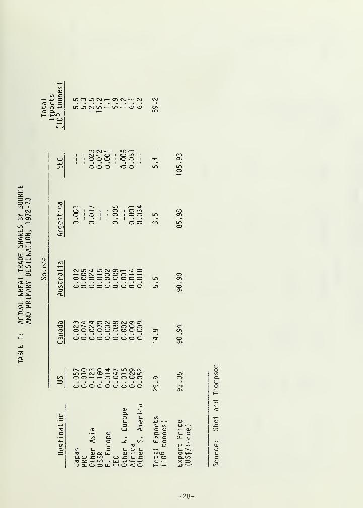
For comparison, Table I shows actual trade shares and prices for

1972-73 and Table II shows trade shares and prices under the perfectly

competitive (free trade) market conduct assumption. Table II exhibits

the classic characteristics of a competitive spatial equilibrium

model. Net trade levels for particular countries are in fair agreement

with the actual levels; but the trade flows between specific countries

are generally inconsistent with the actual flows. The competitive

equilibrium model shows far fewer non-zero trades than in actuality.

In that model Australia, Argentina, and the EEC each serve only one

-17-

consuraer as opposed to many in actuality. The predicted export prices

are in fair agreement, however.

For comparison, the trade share matrix associated with the duopoly

18market conduct assumption is presented in Table III. Note that

there are many more non-zero trades in this case than in the free

trade case (Table II). Also, the trade shares from each of the duo-

polists are in "reasonable" agreement with actual trade (Table I).

However, trade from Australia, Argentina and the EEC are quite dif-

ferent than in actuality (compare Table III and Table I). Export

prices presented in Table III are also in "reasonable" agreement with

Table I.

We now move to the question of quantifying model performance in ex-

plaining trade. Our fundamental goal is to determine which model, if

any, can be judged statistically acceptable in explaining trade. To do

this we will present several statistics representing the degree to which

model-predicted trade corresponds to actual trade. Ideally, we would

like a distribution on the forecast trade share matrix so that we could

determine if the mean forecast trade matrix differs in a statistical

sense from actual trade. Unfortunately, we do not have a distribution

on forecast trade shares. For each conduct assumption we have a single

deterministic forecast trade matrix to compare to a single actual trade

matrix. We do not consider multiple time periods, which might be use-

ful for imputing a distribution for the trade matrices. Nevertheless,

it is still possible to qualitatively compare the matrices and, using

some moderate assumptions, statistically compare the matrices and test

our hypotheses of market conduct. We use two measures to compare fore-

casted trade shares with the base level of trade: the Theil inequality

-18-

coefficient and the Spearman rank correlation coefficient. The Theil

coefficient is not a statistic in the sense of hypothesis testing but

can be used to obtain a qualitative estimate of goodness-of-f it . The

Spearman coefficient can be used for hypothesis testing if (after

Teigen) we pair corresponding elements of the actual and predicted

trade matrices and then treat the resulting set of pairs as a sample

u- . . 19from a bivariate population.

The Theil inequality coefficient (as defined in Theil) has been

widely used to compare forecasts with actual values. Much insight can

be gained using the inequality coefficient but it cannot be used for

hypothesis testing in our case because it is not distribution free.

The inequality coefficient (U) is in essence the root-mean-squared

error between elements of the predicted and actual trade matrices, nor-

malized so that the coefficient lies between zero and one. Perfect

prediction is associated with a zero inequality coefficient. Further

s cinsight is gained by calculating the variance (U ) and covariance (U )

proportions of the inequality coefficient. These two proportions sum

20to unity. Suppose predicted values are plotted against actual

values. For perfect forecasting, all points would lie along a 45°

line. The variance proportion indicates the extent to which the slope

of a regression line through the points deviates from one. The co-

variance proportion indicates the spread of points about this regres-

sion line. Thus, the closer the covariance proportion is to a maximum

of one, the better the forecast since the variance proportion would

then be small, and one would expect some random component in forecasts.

-19-

A second statistic we use is the Spearman rank correlation coeffi-

cient (see Conover), which is a nonparametric statistic. Pairing each

element of the actual (A) and predicted (P) trade matrices, we can view

21these pairs (a.., p..) as samples from a bivariate distribution.

ij ij

Regressing p. . against a. . we obtain a. .= a + p. . + e

. . . We canij ij iJ ij ij

test the null hypothesis that a = and 3=1 (i.e., that the model is

a perfect predictor). However, the elements of the predicted trade

matrix are not independent nor is there a conventional population from

which the (a.., p..) pairs are drawn. Nevertheless, this statistic andij ij

the Theil inequality coefficient should give us a strong foundation on

which to test our hypothesis of the performance of the four models of

market conduct.

With regard to the hypotheses of market conduct, Table IV shows the

two measures of consistency between actual trade shares and simulated

trade shares under the four market conduct assumptions. Note that for

both the Theil and Spearman statistics, the duopoly and triopoly market

conduct assumptions perform considerably better than either the free

trade or EEC-Japan duopsony conduct assumptions. The Theil inequality

coefficient and the variance proportion are considerably lower in the

two oligopoly cases. However, the Spearman rank correlation coefficient

paints a slightly different picture, suggesting that the free trade

conduct assumption behaves fairly well. However, one must interpret

the Theil and Spearman statistics in conjunction with one another. The

Spearman coefficient suggests that the pairs of actual and predicted

shares for free trade lie nicely along the 45° line. In fact, the

three models (all except duopsony) perform similarily on this count.

-20-

However the Theil inequality coefficient suggests that free trade gives

much greater dispersion about this 45° line than do the oligopoly models

,

Thus taking the two statistics together points to the superiority of

the two oligopoly models with the duopoly model performing best.

We turn now to testing hypotheses of market conduct. Our null

hypothesis is that a model predicts trade. More specifically, if one

regresses actual trade against predicted trade (a.. = a+ 3p. . + £..),ij ij ij

the hypothesis is that (ot,0) = (0,1): that actual and predicted trade

are the same, except for a zero-mean error. Our goal then is to

reject the hypothesis for some of the conduct assumptions. At the 90

percent level we can reject the null hypothesis for all except the

duopoly model. At the 95 percent and 99 percent level, we can only

reject the hypothesis for the duopsony model. Thus on all counts, the

duopsony model performs very poorly.

V. CONCLUSIONS

Probably the most significant contribution of this paper is our

development of a model of spatial imperfectly competitive equilibrium.

The approach increases the applicability of spatial equilibrium models

to markets that can be characterized as reaction-function oligopolies/

oligopsonies, and even offers promise for formulating conventional

competitive spatial equilibrium models. The methodology is relatively

easy to implement and, in terms of computer time, quite efficient.

Another contribution of the paper lies in testing three imper-

fect competition models of the international wheat market, models that

have received considerable attention in the literature. While the

-21-

three models (duopoly, triopoly and duopsony) were suggested by

McCalla (1966), Alaouze et al (1978) and Carter and Schmltz (1979),

respectively, these authors do not necessarily assume Cournot-Nash

price discriminating behavior. Nevertheless, we were able to demon-

strate that the duopsony conduct assumption is a very poor explainer of

trade. The duopoly and triopoly models performed considerably better,

with the duopoly model forecasts being slightly closer to the actual

values than the triopoly model.

-22-

FOOTNOTES

Department of Economics, University of Illinois, and EconomicsGroup, Los Alamos National Laboratory, respectively. Work supportedby U.S. Department of Energy and an Arnold 0. Beckman Award. Researchassistance from Gang Yi and comments from Maury Bredahl, Bill Kost,

Lars Mathiesen, Susan Offutt and Phil Paarlberg have been appreciated.

2In fact, by imposing exogeneously specified government policies

on competitive equilibrium models, equilibria can be brought into

better agreement with actual trade patterns.

3There are several possible reasons for this, including the

variety of behavioral models of imperfect competition, each resultingin a different equilibrium level of trade (see Sarris and Schmitz).Further, there have been no generally available computational methodsfor computing spatial equilibrium in imperfect markets.

4There are two classes of models commonly referred to as spatial

equilibrium models. True spatial equilibrium models assume that the

price difference for a commodity at two different locations only needbe exactly equal to transport cost if trade occurs between the twolocations. Equilibrium prices and quantities in such models can be

determined by a variety of methods although mathematical programmingis most frequently used (following methods suggested by Samuelson anddeveloped by Takayama and Judge). In the second class of spatialmodels, the assumption is made that prices at various locations are

related in some fixed manner to a numeraire price. Such models havethe advantage that they are more easily estimated by simultaneousequation methods but the fixed structure of prices is usually only anapproximation to a true competitive price equilibrium.

One might think there is an inconsistency between perfect com-petition and trade policies or barriers. However, as long as thereare many price taking producers and consumers, free entry and exit and

trade barriers are considered totally exogenous , then the model of

perfect competition is still appropriate.

Brock and Magee actually outline the process in the United Stateswhereby an industrial group can induce the government to impose tradepolicies that are in the group's interest.

It should be noted that the duopoly and triopoly models of thewheat market suggested by McCalla and Alaouze et al. are really co-operative oligopolies and thus basically cartels. In their modelsthey assume an agreement exists among the oligopolists regardingpricing and sharing of demand. Carter and Schmitz are not very spe-cific about the operation of a wheat duopsony although they toosuggest some sort of cooperative arrangement.

-23-

8It is generally difficult to compute market equilibria in non-

competitive situations. Recently, Spence has shown how the com-putation of equilibrium in some monopolisitically competitive marketscan be reduced to the maximization of a single function. Murphy et

al. have proposed an iterative method for computing a Nash equilibriumfor an oligopoly by way of a sequence of mathematical programs. It

has been known for some time that equilibrium in the case of a puremonopoly (or monopsony) can be determined by maximizing producer (orconsumer) surplus (Takayama and Judge).

9The idea of using a nonlinear complementarity algorithm to find

an equilibrium in an imperfectly competitive market originated in

discussions between Lars Mathiesen and the first author. Mathiesenwas actually involved in the early stages of formulating the structureof the model presented here and subsequently went on to develop hisown model of international steel trade (Mathiesen, 1983). His contri-butions are appreciated.

The principal algorithm for solving the linear complementarityproblem is due to Lerake and has been implemented by many includingTomlin. A number of algorithms have been proposed for solving thenonlinear complementarity problem (e.g., Mathiesen 1982). It shouldbe noted that in general one is not assured of a unique solution to the

complementarity problem.

Bresnahan's consistent conjectures equilibrium and limit pricingequilibria involve conjectural variations that are themselvesvariables and thus endogenous to the problem.

12Note that we have assumed SPkV^ii = f°r J * k, which means

that by changing shipments to one consumer a producer cannot affectanother consumer's price.

13As in equation (6), here we assume that dc'K /dq-H = for i * k.

The interpretation is that cutbacks in purchaser from one producercannot affect the price of any other producer.

14The transport costs which were used by Shei and Thompson were

not readily available. However, the model resulting from the use of

the transport costs from Sharpies closely approximated the results

reported by Shei and Thompson.

Thus the resulting imperfectly competitive model is actually a

linear complementarity problem, easier to solve than the generalnonlinear complementarity problem.

-i (.

The duopoly, triopoly and duopsony cases are examined becausethey have been suggested by the other authors mentioned earlier in the

paper. However, these authors do not necessarily assume Cournot-Nashbehavior. Thus our models may not correspond exactly to theirs.

The resulting models are quite small, with solution time of up

to 20 CPU seconds on a DEC VAX-11/780 computer (for the triopoly

case)

.

-24-

-1 Q

Teigen assumes that, for a producer-consumer pair, the actualtrade (a) and predicted (p) are sample pairs from a bivariate distri-bution and then calculates the Pearson correlation between a., and p...

However, the Pearson correlation coefficient is not a distribution- J

free statistic and thus is not applicable for testing the relationshipbetween a., and p... The Spearman rank correlation coefficient is

distribution free and thus corrects this problem.

19Trade share matrices for the duopsony and triopoly cases are

available upon request from the authors.

20The bias proportion will be close to zero due to the fact that

elements of the share matrices sum to one.

21Let A and P be the actual and predicted trace matrices, respec-

tively, with elements a-jj and Pi j • Assume each (a-H, Pij) pair is

independent (a strong assumption in our case). Let a and p be the

mean values of a-^-j and Pij computed from the sample. Given the rela-

tionship a-M - a = a + 3 (Pij ~ p) + e ij > we can estimate a and 3.

Since a = and a = p, we wish to test the null hypothesis that 3=1.

To do this, we let u-jj = a^i - p-ji and test the extent of correlation

between u^ i and p£ -j using the Spearman rank correlation coefficient

(p). For our case of a sample of size 45, the null hypothesis can be

rejected if |p| > .248 (at the 90% level) or |p | > .295 (at the 95%

level)

.

-25-

REFERENCES

1. Alaouze, C. M. , Watson, A. S., and Sturgess, N. H. , "OligopolyPricing in the World Wheat Market," Araer. J. Agric. Econ., 60 pp.173-185 (May 1978).

2. Armington, P. S., "A Theory of Demand for Products Distinguishedby Place of Production," International Monetary Fund StaffPapers, _16_(1) pp. 159-176 (March 1969).

3. Breshahan, T. F., "Duopoly Models with Consistent Conjectures,"Amer. Econ. Rev., 71(5) PP» 934-935 (December 1981).

4. Brock, W. A. and Magee, S. P., "The Economics of Special InterestPolitics: The Case of a Tariff," Amer. Econ. Rev., 68 (2 ) pp.246-250 (1978).

5. Carter, C. and Schmitz, A., "Import Tariffs and Price Formationin the World Wheat Market," Amer. J. Agric. Econ., 61 pp. 517-22

(August 1979).

6. Conover, W. J., Practical Nonparametric Statistics 2nd Edition(John Wiley, New York, 1980).

7. Friedman, J., "Oligopoly Theory," in Handbook of MathematicalEconomics , Kenneth J. Arrow and Michael D. Intriligator, Eds.

(North-Holland, Amsterdam, 1982), Chap. II, Vol. II, pp. 491-534.

8. Jeon, D., "A Study of Stability Conditions for the ImperfectWorld Wheat Market: A Duopoly Simulation Model," J. Rural Dev.

,

4_, 37-53 (1981).

9. Johnson, H. G. , "The Gain from Exploiting Monopoly or MonopsonyPower in International Trade," Economica, 3 5 pp. 151-156 (May

1968),

10. Karp, L. S. and McCalla, A. F., "Dynamic Games and InternationalTrade: An Application to the World Corn Market," Amer. J. Agric.

Econ., _65_(4) pp. 641-656 (1983).

11. Lemke, C. E. , "Biamatrix Equilibrium Points and MathematicalProgramming," Mgmt. Sci. _11_, 681-689 (1965).

12. Mathiesen, L., "Complementarity and Economic Equilibrium: A

Modelling Format and an Algorithm (Preliminary Draft)," Dept. of

Operations Research, Stanford University, Stanford, California(January 1982).

-26-

13. Mathiesen, L. , "Modeling Market Equilibria: An Application to

the World Steel Market," unpublished working paper, Center for

Applied Research, Norwegian School of Economics and BusinessAdministration, Bergen, Norway (1983).

14. McCalla, A. F. and Josling, T. E. (eds.), Imperfect Markets in

Agricultural Trade (Allanhed, Osmun & Co., Montclair, NJ , 1981).

15. McCalla, A. F. , "A Duopoly Model of World Wheat Pricing," J. FarmEconomics, _48_ pp. 711-27 (1966).

16. Meilke, K. D. and Griffith, G. R. , "Incorporating Policy Variablesin a Model of the World Soybean/Rapeseed Market," Amer. J. Ag.

Econ., j>5_ pp. 65-73 (Feb. 1983).

17. Morgan, Daniel, Merchants of Grain (Viking, New York, 1979).

18. Murphy, F. H. , Sherali, H. D., and Soyster, A. L. , "A MathematicalProgramming Approach for Determining Oligopolistic MarketEquilibrium," Math. Pgming, 2A_

y pp. 92-106 (1982).

19. Pincus, J. A., Economic Aid and International Cost Sharing , (JohnHopkins, Baltimore, 1965).

20. Pindyck, R. , "Gains to Producers from the Cartelization of

Exhaustible Resources," Rev. Econ. and Stat., 60 pp. 238-251(1978).

21. Rausser, G. C, Litchtenberg, E., and Lattimore, R. , "Develop-ments in Theory and Empirical Application of Endogenous Govern-ment Behavior," Chap. 18 in G. C. Rausser (ed.), New Directionsin Econometric Modelling and Forecasting in US Agriculture(North-Holland, 1982).

22. Salant, S. W. , Imperfect Competition in the World Oil Market(Lexington Books. Lexington, MA, 1982).

23. Sarris, A. H. and Freebairm, J., "Endogenous Price Policies andInternational Wheat Prices," Amer. J. Ag. Econ., 65 pp. 214-224(May 1983).

24. Sarris, A. H. and Schmitz, A., "Price Formation in InternationalAgricultural Trade," in McCalla and Josling (eds.), op. cit.,

Chapter 3.

25. Schmitz, A., McCalla, A. F., Mitchell, D. 0., and Carter, C,Grain Export Cartels (Ballinger, Cambridge, Mass., 1981).

26. Sharpies, J. A., "The Short-Run Elasticity of Demand for US WheatExports," US Dept. of Agriculture, IED Staff Report, Washington,DC (April 1982).

-27-

27. Shei, S-Y. and Thompson, R. L. , "The Impact of Trade Restrictionson Price Stability in the World Wheat Market," Am. J. Ag. Econ.59

, pp. 628-638 (1977).

28. Spence, M. , "The Implicit Maximization of a Function in

Monopolistically Competitive Markets," Harvard Institute of

Economic Research Discussion Paper 461, Cambridge, MA (March1976).

29. Takayama, T. and Judge, G. G. , Spatial and Temporal Price andAllocation Models , (North-Holland, Amsterdam, 1971).

30. Teigen, L. , "Testing a Theoretical Model for World Trade Shares,"Agricultural Economics Research, 29 , (2) 56-59 (1977).

31. Theil, H. , Economic Forecasts and Policy , 2nd Edition (North-Holland, Amsterdam, 1961).

32. Thompson, R. L., "A Survey of Recent US Developments in Inter-national Agricultural Trade Models," US Department of AgricultureEconomic Research Service, Biblio. and Lit. of Ag. Rpt. #21,

Washington, DC (September 1981).

33. Tomlin, J. A., "Robust Implementation of Lemke's Method for the

Linear Complementarity Problem," Systems Optimization LaboratoryReport SOL 76-24, Department of Operations Research, StanfordUniversity, Stanford, California (September 1976).

34. Webb, A.J. , "World Trade in Major US Crops, A Market ShareAnalysis," US Department of Agriculture, Economics and StatisticsService, International Economics Division (April 1981).

D/225

a>t/i c

10 s- ou o *->

O Q.— £CO-. O

in in cm in >— lo i— co co

CM

enin

LUC_)os:o <r>o ^CO I

CM>• r*»

CO CD

COLU •>

< o3: •—

i

co I—«t

LU ZQ .—

i

< h-C£ COI— UJQI—< >-LU CCx <:

< o.=3I— QC_> Z< <

OJ(-)

i-

Cco

UJ_1CO

C_3

ro cm i— in

—

i i c\j i— o i O lo i

i l o O O I O O l

II • . . I . • Io o o o o in

CO

ino

ccuCD

<

rt3

tocto<_>

r— r-» co >— *rO • i

—

I • O I O coO I O I l O I o o• I • I I . I . •

o o o o oin

CO

COCn

in00

cm in «3- in cm co >— «3-oi— O CM >— O O O '—

—

oooooooooOOOOOOOOO

oo^j-^rocMCOCMena^oooooooooooooooooo

in

in

CTi

oen

oen

«3"

en

oen

c^ O c s «a- r-~ in cr> C\J oin r— <^J r_ *d- — CM in in t/>

co o o r— !— o c en CO a.3 • Eo c O o c o c o c CT> CM o

CM CTi sz.

t-

(T3 ccu u (O

<=. a. •^*

O o i~ 00 ^•^ s-

£4-> *—

-

CU CU-u 3 i_ V) CJ -—*. JZ«o to LU <c O CU •r— CU COc r* a) Q. c S_ c*r— 00 Q. • 1 X c Q_ c4-> cC o 3 CO UJ o o • •

i/l i_ re M 4-> 4-> CUCJ c S_ Z3 i_ (J s_ r— i_ ^^ <_>

a <o cu cx UJ CU •^ cu <C<0 o W4- uO.CJ -C LO C-J .C S_ JZ +-> o a. co 3(O a: -M CO • UJ -*-> u- u o r— X o o-D Cu O O LU UJ O < o f— —

-

UJ —

'

CO

-28-

O)c

i~ O oD. S- "^e a. v*I—

i

OO

cr>Lr>co>— >— i>ocoLnco

CO<u

i— ••-> c(O i- o^_> o -»->

O Q.I— SO

—• oQi I—< UJ^: •mi—

i

ccen <a. 2.

- UJz >< 1—

1

1—UJ 1—

H

<_) 1—c: UJZD Q.CZ s:t/J c

C_">-cc >-

_l00 1—UJ oOS UJ< Li-

X es:>y. UJ

Q.

ID Oi— CO CD 00 CO CD CO 00

LT> LD CM "3" O LT) r— IT) V£> f-— f— in

Q ...

<c mi— i

cmI— r-< a

cUJ h-

0)u

o

oo

UJ

(TJ

cCJCD

3

oi r-«. i

l O l

en

CMi co I

I O i CO

00

CM1 ^ 1 1 1 1 1

• •— 1 | 1 | 1

1 • t 1 1 1 1

CM

CC COCD

<T3 r- cc LOc 1 1 KO CD i— 1 1 1 1

to ii O f— O 1 l 1 1 CM

c i i • • 1 1 1 1 •

<T3 o o o lOCD

tO

r~» .— 00CD CD | toO O i o

• IGO O

C CM COI O CM I oI r— O I i—I . • I •

o o o 1^-

CMCOCO

(C

<:a.o

a.os-3UJ

o-_

a;

«T3

-C i.4->

C 1-

<C HI (H L

Q.U3 -C <>0

id o: +J ooOD.CDliJUJO<0 I— -—

to4J --~

o a;CL Cx cUj o

4->

+•> oO f—

aio -—•r- <u- c

CL. Co

»-> -MS- \o **»Q.OOx rziUJ -—

-29-

c+-> a> es_ a oo •<- +->

E Q- *^•—

< 00

r- i- r- O CO Cl CO r- p-

>-

<

CO<D

CO cr- -M c<o s_ o4-> O +->

i-i o

LT) ^- r— CO r— lOr- Lf> Lf> toIT)

o_

o<UJ>.<-> _J

^°oo S

UJ =5

UJ =

"S CT>

c2

CL)

Os-z:

Oc/>

on

coUJ

oUJ

<J) Lf)

1 1 1 1 1 1 1 *fr CO1 I 1 1 1 I 1 o o r^1 1 1 1 1 1 1 • •o o «* oo

C•r—-r->

Cai

ens_<c

Lf)

I I COl I o o

CM enen

fj

+J

coccoLO «T CO IO O O I

o o oI I I I

CM

CC oo

fOcra

o

OOID

in

aj

a

p— uoOi— encooor- cor— r— P^-OOCOOCMi—OOOr— oooooooooooooo

VO^r-CMOC^CMOCMr-CMcri^CMr^CMOOCMOOOr— ooooo

CO COCT>

CO

o o o O O o o o o LC ^_CM en

<TJ

at OQ. •^ 4->

o s_ CO i-L. ai +-> •— o3 E t- CO a. -^*»

<o UJ < o a; X aj•r— a> CL £Z Ul cCO Q. • • x c C< O 3 00 Ul o aj o

L. ra +J en -t->

c s- =3 s_ o s- r— fO <u ^•s^

03 <U CH Ul a> CVI rrjl© s- CJ V»Q-O J= 00 o J= s~ .JZ -t-^ o a> •1

—

ooro CC +-> 00 . UJ -t-> it- •*-> O r— > c rD-0 Q- O 13 Ul u. O 's: o 1— -— <: CL.

-30-

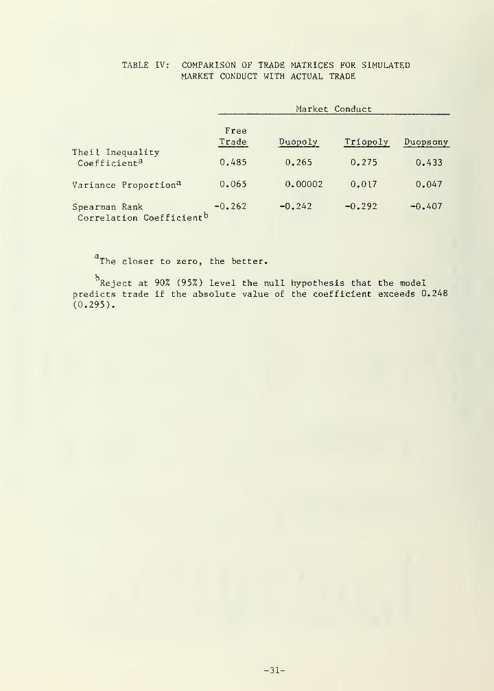
TABLE IV: COMPARISON OF TRADE MATRICES FOR SIMULATEDMARKET CONDUCT WITH ACTUAL TRADE

Market Conduct

FreeTrade Duopoly Triopoly Duopsony

0.485 0.265 0.275 0.433

0.065 0.00002 0.017 0.047

-0.262 -0.242 -0.292 -0.407

Theil InequalityCoefficient3

Variance Proportion3

Spearman RankCorrelation Coefficient^

The closer to zero, the better.

Reject at 90% (95%) level the null hypothesis that the modelpredicts trade if the absolute value of the coefficient exceeds 0.248

(0.295).

-31-

HECKMAN IXIBINDERY INC. |§|

JUN95