Optimal Pricing and Replenishment in a

Single-Product Inventory System

Hong ChenCheung Kong Graduate School of Business, China

Owen Q. Wu∗

Sauder School of Business, University of British Columbia, Canada

David D. Yao†

IEOR Dept., Columbia University, New York, USA

March 1, 2004

Abstract

We study an inventory system that supplies price-sensitive demand modeled by Brownianmotion, focusing on the optimal pricing and inventory replenishment decisions, under bothlong-run average and discounted objectives. Analytical solutions are obtained in all cases,and related to or contrasted against previously known results. In addition, we bring out theinterplay between the pricing and the replenishment decisions, and the way they react todemand uncertainty. We show that the joint optimization of both decisions may result insignificant profit improvement over the traditional way of making the decisions separatelyor sequentially. We also show that multiple price changes will only result in a limited profitimprovement over a single price.

Keywords: Joint pricing-replenishment decision, price sensitive demand, Brownian model.

∗Supported in part by University Graduate Fellowship from the University of British Columbia.†Supported in part by NSF grant DMI-0085124. Part of this author’s research was undertaken while at the

Dept of Systems Engineering and Engineering Management, Chinese University of Hong Kong, and supportedby HK/RGC Grant CUHK4173/03E.

1

1 Introduction

We study a single-product continuous-review inventory model with price-sensitive demand.

The cumulative demand process is modeled by a Brownian motion with a drift rate that is a

function of the price. Replenishment is instantaneous, and demands are satisfied immediately

upon arrival. Consequently, the replenishment follows a simple order-up-to policy, with the

order-up-to level denoted by S.

We allow the pricing decisions to be dynamically adjusted over time. Specifically, we divide

S into N equal segments, with N a given integer. For each segment, there is a price; and all N

prices are optimally determined, jointly with the replenishment level S, so as to maximize the

expected long-run average or discounted profit.

There has been a substantial and growing literature on the joint pricing and inventory con-

trol. We refer the reader to two recent survey papers, Yano and Gilbert (2002), and Elmaghraby

and Keskinocak (2003). Our review below will focus on those works that relate closely to our

study.

Whitin (1955), Porteus (1985a), Rajan et al. (1992), among others, study demands that

are deterministic functions of prices. Whitin (1955) connects pricing and inventory control

in the EOQ (economic order quantity) framework, and Porteus (1985a) provides an explicit

solution for the linear demand instance. Rajan et al. (1992) investigates continuous pricing for

perishable products for which demands may diminish as products age.

Other works study stochastic demand models. Li (1988) considers a make-to-order produc-

tion system with price-sensitive demand. Both production and demand are modeled by Poisson

processes with controllable intensities. The control of demand intensity is through pricing. A

barrier policy is shown to be optimal: when the inventory level reaches an upper barrier, the

production stops; when the inventory level drops to zero, the demand stops (or the demand is

lost). It is also shown that the optimal price is a non-increasing function of the inventory level.

Federgruen and Heching (1999) examines a model in which the firm periodically reviews

inventory and decides both the replenishment quantity and the price to charge over the period.

The replenishment cost is linear, without a fixed setup cost. The prices are changed only at

the beginning of each period (as opposed to the continuous pricing scheme in Rajan et al.

1992). It is shown that a base-stock list-price policy is optimal for both average and discounted

objectives. Earlier related works include Zabel (1972) and Thowsen (1975).

Thomas (1974), Polatoglu and Sahin (2000), Chen and Simchi-Levi (2003a,b), Feng and

2

Chen (2003), and Chen et al. (2003) extend the above model to include a replenishment setup

cost. In the full-backlog setting, it is first conjectured in Thomas (1974), and then proved

in Chen and Simchi-Levi (2003a), that the (s, S, p) policy is optimal for additive demand (a

deterministic demand function plus a random noise) in a finite horizon. Chen and Simchi-

Levi (2003b) further proves the optimalify of the stationary (s, S, p) policy for general demand

in an infinite horizon. Feng and Chen (2003) proves the optimality of (s, S, p) policy under

more general demand functions, but restricting the prices to a finite set. Assuming lost sales,

Polatoglu and Sahin (2000) obtains rather involved optimal policies under a general demand

model and provides restrictive conditions under which the (s, S, p) policy is optimal. Chen et

al. (2003) proves that (s, S, p) policy is optimal under additive demand and lost sales.

Continuous-review models are studied in Feng and Chen (2002), and Chen and Simchi-Levi

(2003c). Feng and Chen (2002) models the demand as a price-sensitive Poisson process. Pricing

and replenishment decisions are made upon finishing serving each demand, but the prices are

restricted to a given finite set. An (s, S, p) policy is proved optimal, with the optimal prices

depending on the inventory level in a rather structured manner. Chen and Simchi-Levi (2003c)

generalizes this model by considering compound renewal demand process with both the inter-

arrival times and the size of the demand depending on the price. It is shown that the (s, S, p)

policy is still optimal.

Our work differs from the above papers in two aspects. First, we model the demand process

by Brownian motion, with a drift term being a function of the price. The Brownian model, with

its continuous path, is appropriate for modeling fast-moving items. It is a natural model when

demand forecast involves Gaussian noises. Furthermore, it allows us to bring out explicitly

the impact of demand variability in the optimal pricing and replenishment decisions, whereas

results along this line are quite limited in the existing literature. (For other works that model

production-inventory systems using Brownian motion, we refer to Puterman (1975) and Har-

rison (1985).) Second, we examine the number of price changes allowed as inventory depletes,

and demonstrate that using a small number of prices, optimally determined, is usually good

enough.

Some of the key findings and new insights from our study include:

• Demand variability incurs an additional inventory holding cost.

• As demand variability increases, the optimal price decreases and the optimal replenish-

ment level increases.

3

• The traditional way of separating the pricing and replenishment decisions could result in

significant profit loss, as compared with the joint decision.

• Multiple price changes will only result in a limited profit improvement over a single price

(when both are optimally determined). The relative improvement, however, becomes

more significant in applications where the profit margin is low.

The rest of the paper is organized as follows. In Section 2, we present a formal description of

our model, in terms of the demand and inventory processes, the cost functions, and the pricing

and replenishment decisions. In Section 3, we study the optimal pricing and replenishment

decisions under the long-run average objective. We start from making these decisions separately,

so as to highlight the comparisons against prior studies and known results, and then present

the joint optimization model and demonstrate the profit improvement. In Section 4, we present

analogous results under the discounted objective, emphasizing the contrasts against the average

objective case. We conclude the paper pointing out possible extensions in Section 5.

2 Model Description and Preliminary Results

We consider a continuous-review inventory model with a price-sensitive demand. The objective

is to determine the inventory replenishment and pricing decisions that strike a balance between

the sales revenue and the cost for holding and replenishing inventory over time, so as to maximize

the expected long-run average or discounted profit. The specifics of the demand model, the

cost parameters and the control policy are elaborated in the following three subsections.

2.1 The Demand Model

The subject of our study is a single-product inventory system supplying a price-sensitive demand

stream. The cumulative demand up to time t is denoted as D(t), and modeled by a diffusion

process:

D(t) =∫ t

0λ(pu)du+ σB(t), t ≥ 0, (1)

where pt is the price charged at time t; λ(pt) is the demand rate at time t, which is a decreas-

ing function of pt; B(t) denotes the standard Brownian motion; and σ is a positive constant

measuring the variability of the demand (or the error of demand forecast).

This Brownian demand model can be related to other discrete (i.e., integer-valued) demand

processes through strong approximation (Csorgo and Horvath 1993). Consider, for instance, a

4

Poisson demand process with an instantaneous rate λ(pt), and write the cumulative demand

as A( ∫ t

0λ(pu)du

), where A(·) denotes the Poisson process with a unit rate. Then the strong

approximation implies that a version of A on a suitable probability space satisfies

sup0≤t≤T

∣∣∣A( ∫ t

0λ(pu)du

)−∫ t

0λ(pu)du−B

( ∫ t

0λ(pu)du

)∣∣∣ = O(log(T )),

where B is a standard Brownian motion defined on the same probability space. If the process

A follows a more general probability law (i.e., not necessarily Poisson), then the order of ap-

proximation will be O(T 1/r) for a constant r ∈ (2, 4). Using Brownian model to approximate

discrete (point) process has been a standard approach in many other applications, stochastic

networks in particular; refer to, e.g., Harrison (1988, 2003), and Chen and Yao (2001).

Let P and L denote, respectively, the domain and the range of the demand rate function

λ(·). Both are assumed to be intervals of <+ (the set of nonnegative real numbers); in addition,

0 6∈ L.

Assumption 1 (on demand rate) The demand rate λ(p) and its inverse p(λ) are both positive-

valued, strictly decreasing, and twice continuously differentiable in the interior of P and L,respectively. The revenue rate r(λ) = p(λ)λ is strictly concave in λ.

Many commonly-used demand functions satisfy the above assumption, including the follow-

ing examples, where the parameters α, β and δ are all positive:

• The linear demand function λ = α−βp, p ∈ [0, α/β]: r(λ) = αβλ−

1βλ

2 is strictly concave;

• The exponential demand function λ = αe−βp, p ≥ 0: r(λ) = − 1βλ log(λ/α) is strictly

concave;

• The power demand function λ = βp−δ, p ≥ 0: r(λ) = λ−1δ+1β

1δ is strictly concave if

δ ≥ 1.

2.2 Cost Parameters

Let h be the cost for holding one unit of inventory for one unit of time. Let c(S) be the cost to

replenish S units of inventory.

Assumption 2 (on replenishment cost) The replenishment cost function c(S) is twice con-

tinuously differentiable and increasing in S for S ∈ (0,∞). The average cost a(S) = c(S)/S is

strictly convex in S, and a(S)→∞, as S → 0.

5

Consider a special case: c(S) = K + cSδ, S > 0, where K, c, δ > 0. When δ = 1, this

is the most commonly used linear function with a setup cost K. The average cost function,

a(S) = KS + cSδ−1 is convex if δ ∈ (0, 1] ∪ [2,∞]. Furthermore, as we shall demonstrate below,

when S satisfies a′(S) ≤ 0, which is the primary case of interest, a(S) is convex for all δ > 0.

To see this, consider δ ∈ (1, 2), and note that

a′(S) =1S2

(−K + c(δ − 1)Sδ);

and when a′(S) ≤ 0, we have

a′′(S) = −2− δS3

(− 2

2− δK + c(δ − 1)Sδ

)≥ −a

′(S)(2− δ)S

≥ 0.

2.3 Pricing and Replenishment Policies

Assume replenishment is instantaneous, i.e., with zero leadtime. We further assume that all

orders (demand) will be supplied immediately upon arrival; i.e., no back-order is allowed, or

there is an infinite back-order cost penalty. (Our results extend readily to the back-order case;

refer to Section 5.)

The replenishment follows a continuous-review, order-up-to policy. Specifically, whenever

the inventory level drops to zero, it is brought up to S instantaneously via a replenishment,

where S is a decision variable. We shall refer to the time between two consecutive replenishments

as a cycle.

We adopt the following dynamic pricing strategy. Let N ≥ 1 be a given integer, and let

S = S0 > S1 > · · · > SN−1 > SN = 0. Immediately after a replenishment at the beginning

of a cycle, price p1 is charged until the inventory drops to S1; price p2 is then charged until

the inventory drops to S2; ...; and finally when the inventory level drops to SN−1, price pN is

charged until the inventory drops to SN = 0, when another cycle begins. The same pricing

strategy applies to all cycles. For simplicity, we set Sn = S(N − n)/N . That is, we divide the

full inventory of S units into N equal segments, and price each segment with a different price

as the inventory is depleted by demand.

In summary, the decision variables are: (S,p), where S ∈ <+, and p = (p1, . . . , pN ) ∈ PN .

Within a cycle, we shall refer to the time when the price pn is applied as period n.

2.4 The Inventory Process

Without loss of generality, suppose at time zero the inventory is filled up to S. We focus on

the first cycle which ends at the time when inventory reaches zero. Let T0 = 0, and let Tn be

6

the first time when inventory drops to Sn:

Tn := inf{t ≥ 0 : D(t) = nS/N}, n = 1, 2, . . . , N.

The length of period n is therefore τn := Tn − Tn−1. Since Tn’s are stopping times, by the

strong Markov property of Brownian motion, τn is just the time during which S/N units of

demand has occurred under the price pn. That is,

τndist.= inf{t ≥ 0 : λ(pn)t+ σB(t) = S/N}. (2)

Let X(t) denote the inventory-level at t. We have,

X(t) = S −D(t), t ∈ [0, TN ).

Since our replenishment-pricing policy is stationary, X(t) is a regenerative process with the

replenishment epochs being its regenerative points.

We conclude this section with a lemma, which gives the first two moments and the generating

function of the stopping time τn. (The proof is in the appendix.)

Lemma 2.1 For the stopping time τn in (2), we have

E(τn) =S

Nλn, (3)

E(τ2n) =

σ2

λ2n

E(τn) + E2(τn) =σ2S

Nλ3n

+S2

N2λ2n

, (4)

E(e−γτn) = exp[−√

λ2n+2σ2γ−λn

σ2SN ], (5)

where λn = λ(pn) > 0, and γ > 0 is a parameter.

3 Long-Run Average Objective

To optimize the long-run average profit, thanks to the regenerative structure of the inventory

process, it suffices for us to focus on the first cycle. Recall that period n refers to the period in

which the price pn applies, and the inventory drops from Sn−1 = (N−n+1)SN to Sn = (N−n)S

N . We

first derive the total inventory over this period. Applying integration by parts, and recognizing

dX(t) = −dD(t), X(Tn−1) = Sn−1, X(Tn) = Sn,

7

we have∫ Tn

Tn−1

X(t)dt = TnSn − Tn−1Sn−1 −∫ Tn

Tn−1

tdX(t)

= TnSn − Tn−1Sn−1 −∫ Tn

Tn−1

Tn−1dX(t) +∫ Tn

Tn−1

(t− Tn−1)dD(t)

= τnSn +∫ Tn

Tn−1

(t− Tn−1)[λ(pn)dt+ σdB(t)

].

A simple change of variable yields∫ Tn

Tn−1

(t− Tn−1)λ(pn)dt =∫ τn

0uλ(pn)du =

12λ(pn)τ2

n;

whereas

E

[ ∫ Tn

Tn−1

(t− Tn−1)dB(t)]

= E

[ ∫ Tn

Tn−1

tdB(t)]− E

[Tn−1

]E[B(Tn)−B(Tn−1)

]= 0,

follows from the martingale property of B(t) and the optional stopping theorem.

Let vn(S, pn) denote the expected profit (sales revenue minus inventory holding cost) during

period n. Then, making use of the above derivation, along with Lemma 2.1, we have

vn(S, pn) =pnS

N− E

[ ∫ Tn

Tn−1

hX(t)dt]

=pnS

N− hE[τn]Sn −

12hλ(pn)E[τ2

n]

=pnS

N−hS2(N − n+ 1

2)N2λ(pn)

− hσ2S

2Nλ(pn)2, (6)

Note in the above expression, the first term is the sales revenue from period n, the second term

is the inventory holding cost attributed to the deterministic part of the demand (i.e., the drift

part of the Brownian motion), and the last term is the additional holding cost incurred by

demand uncertainty.

For ease of analysis, below we shall often use {µn = λ(pn)−1, n = 1, . . . , N} as decision

variables and denote µ = (µ1, . . . , µN ) ∈ MN and M = {λ(p)−1 : p ∈ P}. Then, the long-run

average objective can be written as follows:

V (S,µ) =∑N

n=1 vn(S, pn)− c(S)SN

∑Nn=1 µn

=

∑Nn=1

[p( 1

µn)− hS

N (N − n+ 12)µn − hσ2

2 µ2n − a(S)

]∑N

n=1 µn

. (7)

The additional holding cost due to demand uncertainty is represented by hσ2∑N

n=1 µ2n

2∑N

n=1 µn.

8

For the special case when N = 1, the price and the demand rate are both constants in a

cycle (and hence constant throughout the horizon). The objective function (7) takes a simpler

form. For comparison with some classical work, we use λ as the decision variable and denote

the long-run average profit under single-price policy as V (S, λ). Then,

V (S, λ) =v1(S, p(λ))− c(S)

S/λ= r(λ)− hS

2− λa(S)− hσ2

2λ. (8)

The classical EOQ model only consists of the second and third terms in (8), which are the total

cost if the demand is deterministic with a constant rate. Whitin (1955) and Porteus (1985a)

considered the price-sensitive EOQ model, which involves the first three terms in (8). Our

model gives rise to an additional holding cost due to demand variability.

3.1 Optimal Replenishment with Fixed Prices

In this case, the set of prices p, or equivalently, µ is given, and the firm’s problem is

maxS>0

V (S,µ).

Under Assumption 1, V (S,µ) is strictly concave in S. Note that V (S,µ)→ −∞ as S →∞ or

S → 0 (the latter is due to Assumption 2 that a(S)→∞ as S → 0). Thus, the unique optimal

replenishment level is determined by the first-order condition:

S∗ = a′−1(− h

N2

N∑n=1

(N − n+12)µn

), (9)

where a′−1 is well-defined since a(·) is strictly convex and a′(·) is strictly increasing under As-

sumption 2. In practice, the average cost as a function of quantity is usually first decreasing

(due to economy of scale) and then increasing (due to capacity or other technological restric-

tions). However, at the optimal replenishment level, we have a′(S∗) < 0 for any fixed prices.

This observation helps to reduce the search space when the replenishment level is optimized

jointly with pricing decisions (see Section 3.3).

The way that the demand variability and the holding cost impact the optimal replenishment

level can be readily derived from (9).

Proposition 3.1 With prices fixed,

(i) the optimal replenishment level S∗ is independent of σ, and decreasing in h and in pn (for

any n);

(ii) the optimal profit is decreasing in σ and h.

9

Proof. Part (i) is obvious from (9). (Note, in particular, that the additional holding cost due

to demand variability is independent of the replenishment level.) For (ii), consider σ1 ≤ σ2,

and denote the corresponding maximizers as S∗1 and S∗2 and the objective values as V (S∗1 ,µ, σ1)

and V (S∗2 ,µ, σ1), respectively. We have V (S∗1 ,µ, σ1) ≥ V (S∗2 ,µ, σ1) ≥ V (S∗2 ,µ, σ2), where the

first inequality is due to the maximality of S∗1 and the second one follows immediately from the

objective function in (7). The case of decreasing in h is completely analogous.

Example 3.1 Consider the linear replenishment cost: c(S) = K + cS, where K, c > 0. The

first order condition in (9) leads to the familiar EOQ formula:

S∗ =

√2Kλa

h, where λa =

( N∑n=1

2N − 2n+ 1N2

µn

)−1. (10)

In the standard EOQ model, the demand rate is taken as the average demand per time unit,

which in our setting becomes

λ =( 1N

N∑n=1

µn

)−1. (11)

Suppose that the fixed prices satisfy p1 ≤ p2 ≤ · · · ≤ pN (or µ1 ≤ µ2 ≤ · · · ≤ µN ), i.e.,

a lower price is charged when the inventory level is higher (we will see this price pattern in

Proposition 3.3). Higher weights are given to smaller µn’s in (10), while µn’s are equally

weighted in (11). Hence, λ ≤ λa. This implies that the standard EOQ with a time-average

demand rate may lead to a replenishment level lower than the optimally desirable.

Example 3.2 Let c(S) = 100 + 5S, λ(p) = 50 − p, h = 1 and N = 1. In Figure 1(a), the

EOQ quantity is shown as a function of the single fixed price, S∗ = 10√

100− 2p. Figure 1(b)

illustrates the optimal profit corresponding to various levels of demand variability. The peak of

each V ∗ curve is reached when both the price and the replenishment level are jointly optimized.

When the price deviates far away from the optimum, the profit falls dramatically.

Figure 1: Optimal replenishment with a fixed price

10

3.2 Optimal Pricing with a Fixed Replenishment Level

3.2.1 The Single-Price Problem

Here N = 1. We want to optimize the single price, or equivalently, the demand rate, as follows:

maxλ∈L

V (S, λ) = r(λ)− hS

2− λa(S)− hσ2

2λ.

Under Assumptions 1 and 2, V (S, λ) is strictly concave in λ. Assuming an interior solution

(which is rather innocuous, since the last two terms in the objective forbid λ to be extreme),

the unique optimal λ follows from the first-order condition:

r′(λ) +hσ2

2λ2= a(S). (12)

We have the following proposition.

Proposition 3.2 Suppose a single price is optimized while the replenishment level is held fixed.

(i) If the optimal price p∗ is in the interior, then the marginal revenue at p∗ is no larger than

the average replenishment cost, i.e., r′(λ(p∗)) ≤ a(S).

(ii) The optimal price p∗ is decreasing in σ and h.

(iii) The optimal price p∗ is increasing in a(·); if a(S) is decreasing in S, then p∗ is decreasing

in S.

(iv) The optimal profit is decreasing in σ and h.

Proof. The statement in (i) follows immediately from (12). For (ii) and (iii), note that∂2V∂λ∂σ = hσ

λ2 > 0, ∂2V∂λ∂h = σ2

2λ2 > 0, and ∂2V∂λ∂(a(S)) = −1 < 0. That is, the objective function

V is supermodular in (λ, σ), supermodular in (λ, h) and submodular in (λ, a(S)). Hence, (ii)

and (iii) follow from standard results for super/submodular functions (Topkis 1978). For (iv),

follow a similar argument to the one that proves Proposition 3.1 (ii).

Example 3.3 If λ(p) = βp−1, c(S) = K + cS, where β,K, c > 0, then r(λ) = β, and the

first-order condition (12) becomeshσ2

2λ2=K

S+ c,

leading to the optimal price

p∗ =β

λ∗=β

σ

√2(K

S + c)h

,

which is clearly decreasing in σ, h and S.

11

Example 3.4 If λ(p) = α − βp, where α, β > 0, then r(λ) = (α − λ)λ/β, and the first-order

condition in (12) becomes

α− 2λβ

+hσ2

2λ2= a(S),

which can be simplified to

f(λ) ≡ 4λ3 + 2[βa(S)− α]λ2 − hβσ2 = 0.

Note that f(0) < 0, f(+∞) = +∞, f ′(λ) = 4λ[3λ + βa(S) − α]; hence, f(λ) is either strictly

increasing or first decreasing and then increasing. In either case, the above equation has a

unique solution λ∗ in (0,∞). If λ∗ ≤ α, it is the optimal demand rate, and the optimal price

is p∗ = (α − λ∗)/β. If λ∗ > α, it can be shown that V is increasing in λ for λ ∈ [0, λ∗], and

therefore the optimal demand rate is α and the optimal price is zero.

If σ or h increases or a(·) decreases, then f(λ) decreases for any λ; and consequently, λ∗

increases. This illustrates the monotonicity in (ii) and (iii) of Proposition 3.2.

Example 3.5 Under the same setting as Example 3.2, Figure 2 plots the optimal price and

the corresponding profit against various levels of replenishment and demand variability. The

results depict the qualitative trends in Proposition 3.2. The peak of each V ∗ curve is reached

when the price and inventory are jointly optimized. In contrast to Figure 1(b), the profit here

appears less sensitive to the replenishment level, as long as the pricing decision is optimized.

Figure 2: Optimal price with a fixed replenishment level

3.2.2 The N-Price Problem

In this case, the decision variables are the set of prices p, or equivalently, µ. Specifically, the

problem is

maxµ∈MN

V (S,µ) =

∑Nn=1

[p( 1

µn)− hS

N (N − n+ 12)µn − hσ2

2 µ2n − a(S)

]∑N

n=1 µn

. (13)

The strict concavity of the revenue function r(λ) (Assumption 1) implies that the function

p( 1µ) is strictly concave in µ. This is because r′′(λ) = 2p′(λ) + λp′′(λ) and d2p( 1

µ)/dµ2 =1µ3 (2p′( 1

µ)+ 1µp

′′( 1µ)) have the same sign. Thus, the numerator of the objective is strictly concave

in µ. The ratio of a positive concave function over a positive linear function is known to be

12

pseudo-concave (Mangasarian 1970). Hence, V (S,µ) is pseudo-concave in µ. Furthermore, it

is strictly pseudo-concave in the sense that

∇µV (S,µ1)(µ2 − µ1) ≤ 0 ⇒ V (S,µ2) < V (S,µ1). (14)

Hence, the optimal µ must be unique. (This follows from a straightforward extension of Man-

gasarian (1970) from pseudo-concavity to strict pseudo-concavity.) Suppose the optimality is

achieved at an interior point. Then the optimal µ is uniquely determined by the first-order

condition:

∂vn(S, µn)∂µn

=∑N

k=1 vk(S, µk)− c(S)∑Nk=1 µk

, n = 1, . . . , N, (15)

where vn(S, µn) = vn(S, p( 1µn

)). Note that the right side of the above does not depend on n.

This implies that the optimal pricing must be such that the marginal profit is the same across

all periods (assuming an interior optimum).

The following proposition describes the basic optimal pricing pattern.

Proposition 3.3 For any replenishment quantity S, the optimal prices are increasing over the

periods, i.e., p∗1 ≤ p∗2 ≤ · · · ≤ p∗N .

Proof. Since pn = p( 1µn

) is increasing in µn, it suffices to show that the optimal µ∗n is increasing

in n. But this follows immediately from (13), since given any (µ1, . . . , µN ), rearranging these

variables (but not changing their values) in increasing order will maximize the term∑N

n=1 nµn

in the numerator, while all other terms remain unchanged.

Hence, within each cycle, the optimal prices are increasing over the periods. The following

lemma gives an inequality to bound the price increments. The inequality can be derived from

the equal marginal profit property, but it still holds without the interior optimum assumption,

and its proof is in the appendix.

Lemma 3.1 For fixed S, let µ∗ be the optimal N prices. Then for 1 ≤ m < n ≤ N ,

µ∗n − µ∗m ≤ S(n−m)N(σ2 + B

h

) ≤ S(n−m)Nσ2

,

where B = inf{−

d2p( 1µ

)

dµ2 : µ ∈ [µ∗1, µ∗N ]}.

Next we explore the impact of the parameters, σ, h and S on the optimal prices. We shall

write µ∗(σ), µ∗(h) and µ∗(S) to emphasize the dependence of the maximizer of (13) on these

parameters. The proof of the next lemma is also in the appendix.

13

Lemma 3.2 Assuming interior optimum,

(i) µ∗(σ) is differentiable and dµ∗n(σ)dσ < 0 if and only if

N∑k=1

µ∗k(σ)2 − 2µ∗n(σ)N∑

k=1

µ∗k(σ) < 0; (16)

(ii) µ∗(h) is differentiable and dµ∗n(h)dh < 0 if and only if

S

N

N∑k=1

(n− k)µ∗k + σ2N∑

k=1

(µ∗k2

2− µ∗nµ∗k

)< 0. (17)

(iii) µ∗(S) is differentiable and dµ∗n(S)dS < 0 if and only if

h

N2

N∑k=1

(n− k)µ∗k(S) < −a′(S); (18)

The results provided in the above lemma are local, in the sense that they only hold for

parameter values that satisfy the specific conditions in question. Nevertheless, for µ1 and µN

some of these results can be strengthened; see (i)-(iii) of the following proposition.

Proposition 3.4 Assuming interior optimum,

(i) The highest price p∗N (σ) is decreasing in σ.

(ii) The lowest price p∗1(h) is decreasing in h.

(iii) If a′(S) < 0, then p∗1(S) is decreasing in S;

(iv) The optimal profit is decreasing in σ and h.

Proof. (i) By Lemma 3.2, the inequality in (16) always holds for n = N , as µ∗N is the largest

component of µ following Proposition 3.3. Hence µ∗N is decreasing in σ.

(ii) Denote the left side of (17) by Ln. We will show that L1 + LN < 0 and L1 < LN , which

then implies L1 < 0.

L1 + LN =S

N

N∑k=1

(N + 1− 2k)µ∗k + σ2N∑

k=1

[µ∗k

2 − (µ∗1 + µ∗N )µ∗k]

=S

N

[(N − 1)(µ∗1 − µ∗N ) + (N − 3)(µ∗2 − µ∗N−1) + · · ·+ (µ∗bN

2c − µ

∗bN+3

2c)]

+ σ2N∑

k=1

[µ∗k(µ

∗k − µ∗N )− µ∗1µ∗k

]< 0,

14

where the last inequality follows from µ∗n increasing in n. Next, note that

L1 − LN =[S(1−N)

N+ σ2(µ∗N − µ∗1)

] N∑k=1

µ∗k ≤ 0,

where the last inequality follows from Lemma 3.1. Hence L1 < 0, and p∗1(h) is decreasing in h.

(iii) By Lemma 3.2, if a′(S) < 0 and n = 1, the inequality in (18) always holds. Hence µ∗1 is

decreasing in S.

(iv) The proof is completely analogous to the proof for Proposition 3.1 (ii).

The proof of part (i)-(iii) of the above proposition relies on the interior optimum assumption

in Lemma 3.2, but we find through numerical tests that these monotonicity results hold even

without the interior optimum assumption. The next example illustrates Proposition 3.3 and

3.4 and provides comparison plots for Propositions 3.4 and 3.2.

Example 3.6 (a) Let p(λ) = 50 − 10λ, c(S) = 500 + 5S, S = 100, h = 2, and let σ vary

from 0 to 20. For N = 4, the optimal prices are plotted in Figure 3 (a). The highest price is

decreasing in σ while the others are not. There also exist other instances in which all the prices

are decreasing in σ. The demand variability incurs additional holding cost hσ2∑

µ2n∑µ . When σ

increases, in order to balance out the increase of this cost, intuitively we need to decrease µ

and at the same time decrease the spread of µ (i.e., µN − µ1). The composite effect is mixed

except for µ∗N .

(b) Let p(λ) = 50 − 10λ, c(S) = 500 + 5S, S = 100, σ = 1, and let h vary from 0 to 3. The

optimal prices are shown in Figure 3 (b). The lowest price is decreasing in h while the others

are not. The spread of the prices increases significantly with the increase in h.

(c) Let p(λ) = 50 − λ, c(S) = 100 + S, h = 0.5, σ = 3, and let S vary from 0 to 400. The

optimal prices are shown in Figure 3 (c). Note that a′(S) < 0 for all S. The lowest price is

decreasing in S while the others are not. The spread of the prices increases in S.

Figure 3: Optimal N prices and optimal single price

All the above examples show p∗1 < · · · < p∗N . For comparison, the optimal price for the

single-price problem are also plotted as p∗ in Figure 3.

Dynamic pricing obviously produces more profit than using a single fixed price, since the

latter is a special case of the dynamic pricing strategy. To quantify the potential benefit of

dynamic pricing is the purpose of the following proposition.

15

Proposition 3.5 For fixed S, let µ∗ be the optimal N prices, and let V ∗N be the optimal average

profit defined in (13). Then,

V ∗N − V ∗1 ≤hS2

(1−N−2

)12µ

(σ2 + B

h

) ,where µ = 1

N

∑Nn=1 µ

∗n and B = inf

{−

d2p( 1µ

)

dµ2 : µ ∈ [µ∗1, µ∗N ]}.

Proof. We consider a feasible single-price policy that charges a price p(µ−1), and compare

this with the optimal N -price policy. We show the latter has a lower average revenue, a higher

additional holding cost due to demand variability, and the same average ordering cost. Hence,

for the optimal N -price policy to yield a higher profit, it must have a lower average holding

cost attributed to the deterministic part of the demand. By the same reasoning, the difference

between these two average holding-cost terms corresponding to the two policies constitute an

upperbound on the improvement from the single-price policy to the N -price policy.

Specifically, the average profit of charging a single price p(µ−1) is

V1 =p( 1

µ)− hS2 µ−

hσ2

2 µ2 − a(S)

µ.

We have

V ∗N − V ∗1≤ V ∗N − V1

=

∑Nn=1

[p( 1

µ∗n)− p( 1

µ)]− hS

N

∑Nn=1

[(N − n+ 1

2)µ∗n − N2 µ)

]− hσ2N

2

[1N

∑Nn=1 µ

∗2n − µ2

]∑N

n=1 µ∗n

The first term in the numerator,∑N

n=1

[p( 1

µ∗n)− p( 1

µ)]≤ 0, since p( 1

µ) is concave in µ; and

the last term in the numerator 1N

∑Nn=1 µ

∗2n − µ2 ≥ 0, which is essentially the Cauchy-Schwartz

inequality. Thus,

V ∗N − V ∗1 ≤−hS

N

∑Nn=1

[(N − n+ 1

2)µ∗n − N2 µ)

]∑Nn=1 µ

∗n

=hS

N

(∑Nn=1 nµ

∗n∑N

n=1 µ∗n

− N + 12

)

=hS

N

(2µ∗1 + 4µ∗2 + · · ·+ 2Nµ∗N − (N + 1)(µ∗1 + · · ·+ µ∗N )

2∑N

n=1 µ∗n

)

=hS

N

((N − 1)(µ∗N − µ∗1) + (N − 3)(µ∗N−1 − µ∗2) + . . .

2Nµ

)16

where in the last line, the series ends with µ∗N/2+1−µ∗N/2 ifN is even, and ends with 2

(µ∗(N+3)/2−

µ∗(N−1)/2

)if N is odd.

Applying Lemma 3.1 and the identity:

(N − 1)2 + (N − 3)2 + · · ·+ (N + 1− 2⌊N

2

⌋)2 =

(N − 1)N(N + 1)6

,

we have

V ∗N − V ∗1 ≤ hS2

µ(σ2 + B

h

) ((N − 1)2 + (N − 3)2 + · · ·+ (N + 1− 2bN2 c)2

2N3

)

=hS2

µ(σ2 + B

h

) (N − 1)N(N + 1)12N3

=hS2

(1−N−2

)12µ

(σ2 + B

h

) .The bound in the above proposition indicates that the N -price policy cannot improve much

over the single-price policy when the replenishment quantity and the holding cost are low and

the demand variability is high.

Also note that this bound does not rely on the interior optimum assumption. It will be used

in the next section to derive a bound on improvement for the joint pricing and replenishment

strategy.

3.3 Joint Pricing-Replenishment Optimization

3.3.1 One Price

In this case, the firm’s problem is

maxS>0, λ∈L

V (S, λ) = r(λ)− hS

2− λa(S)− hσ2

2λ. (19)

The first-order conditions are given by (9) and (12). The difficulty is, V (S, λ) may not be

concave in (S, λ), and it may even have multiple local maxima (see Example 3.7 below). How-

ever, under linear demand and linear replenishment cost, a solution satisfying the first order

conditions and yielding positive profit must be the global optimum, as demonstrated below.

Proposition 3.6 Suppose λ(p) = α− βp, c(S) = K + cS, where α, β,K, c > 0. If S∗ > 0 and

λ∗ ∈ (0, α] satisfy the first-order conditions in (9) and (12), and V (S∗, λ∗) > 0, then (S∗, λ∗)

solves problem (19).

17

Proof. From Example 3.1, the optimal replenishment level for each λ is S∗(λ) =√

2Kλ/h.

We replace S in the objective by S∗(λ), and then find the optimal λ. Let

W (λ) := V (S∗(λ), λ) = (α− λ)λ/β − cλ−√

2Khλ− hσ2

2λ.

We prove that λ∗ satisfying W ′(λ∗) = 0 and W (λ∗) > 0 is the global maximizer.

Let f(λ) := (α − λ)λ/β − cλ −√

2Khλ. It is easy to see that f(0) = 0, f ′(0) = −∞ and

f ′′(λ) = − 2β +

√hK8λ3 . Let λ be the inflection point, i.e., f ′′(λ) = 0. Then, f(λ) starts decreasing

from zero, is convex in [0, λ] and concave in [λ,∞).

Suppose f ′(λ) ≤ 0, then by convexity/concavity, f ′(λ) ≤ f ′(λ) ≤ 0 for all λ ≥ 0. Therefore,

W (λ) < f(λ) ≤ f(0) = 0 for all λ ≥ 0, so there exists no maximizer with positive profit in this

case. Hence, we must have f ′(λ) > 0.

Next, let λ1 be the local minimizer for f(λ) in the convex part of the function. Obviously,

λ1 < λ. First, λ∗ 6∈ [0, λ1] because in this region W (λ) < f(λ) ≤ 0. Second, λ∗ 6∈ [λ1, λ] because

in this region W ′(λ) = f ′(λ) + hσ2

2λ2 > 0. Hence, λ∗ ∈ [λ, α]. (λ < α in order for λ∗ to exist.)

Since W (λ) = f(λ) − hσ2

2λ is strictly concave in [λ, α], λ∗ is the unique maximizer for W (λ) in

[λ, α]. It is the global maximizer since all other local maximizers (if any) must be within [0, λ1],

the region where W (λ) < 0.

The following example illustrates multiple local maxima and the above proposition.

Example 3.7 Consider linear demand λ(p) = 50−p, linear replenishment cost c(S) = 500+2S,

σ = 0.2 and h = 1. The optimal S for any fixed λ is given by S(λ) = 10√

10λ. Substituting

this EOQ into the first-order condition (12) gives

50− 2λ+1

50λ2=

5√

10√λ

+ 2.

However, simply solving the above equation yields three stationary points: λ1 = 0.01619,

λ2 = 0.1010, and λ3 = 22.327. Using the second-order condition, it can be verified that λ1 and

λ3 are local maxima, while λ2 is a local minimum. Furthermore, V (S(λ1), λ1) = −4.482 and

V (S(λ3), λ3) = 423.8. Hence λ∗ = λ3 = 22.327 and S∗ = 149.42.

The monotonicity of the joint optimum is explored in the following proposition (compared

with Proposition 3.1 and 3.2 where a single decision is optimized).

Proposition 3.7 If there is a unique optimal price and replenishment level, then

(i) the optimal price is decreasing in σ;

18

(ii) the optimal replenishment level is increasing in σ and decreasing in h;

(iii) the optimal profit is decreasing in σ and h.

Proof. (i) The joint optimization problem can be solved sequentially. We first optimize S for

each fixed λ > 0 (same as Section 3.1). From Proposition 3.1, the optimal S is invariant to σ,

and we denote it by S∗(λ). Then, the optimal λ can be found by

maxλ∈L

V (λ, σ) := r(λ)− hS∗(λ)2

− λa(S∗(λ))− hσ2

2λ.

Now, V (λ, σ) is supermodular in (λ, σ) since

∂2V

∂λ∂σ=hσ

λ2≥ 0,

and therefore λ∗(σ) is increasing in σ, or equivalently, the optimal price is decreasing in σ.

(ii) That S∗ is increasing in σ follows immediately from (i) and Proposition 3.1 (i). To examine

the effect of h on S∗, we first optimize λ for each fixed S > 0 (same as Section 3.2), and denote

the maximizer by λ∗(S, h). Then, the optimal S is determined by

maxS>0

V (S, h) := r(λ∗(S, h))− hS

2− λ∗(S, h)a(S)− hσ2

2λ∗(S, h).

Let λ∗S , λ∗h and λ∗Sh denote the partial derivatives. We have

∂2V

∂S∂h= r′′λ∗Sλ

∗h + r′λ∗Sh −

12− aλ∗Sh − a′λ∗h +

σ2

2λ∗2λ∗S −

hσ2

λ∗3λ∗Sλ

∗h +

hσ2

2λ∗2λ∗Sh

= λ∗S

(r′′λ∗h +

σ2

2λ∗2− hσ2

λ∗3λ∗h

)− 1

2− a′λ∗h +

(r′ − a+

hσ2

2λ∗2)λ∗Sh

Since λ∗(S, h) is uniquely determined by (12), the last term in the above is zero, and

λ∗S =a′

r′′ − hσ2

λ∗3

, λ∗h =− σ2

2λ∗2

r′′ − hσ2

λ∗3

,

Then, the first term in the above is also zero, and we have

∂2V

∂S∂h= −1

2− a′λ∗h = −1

2+

a′ σ2

2λ∗2

r′′ − hσ2

λ∗3

Now we show that the above is less than zero if evaluated at S∗. This is because S∗ satisfies

(9), which implies a′(S∗) = − h2λ∗ , and

∂2V

∂S∂h= −1

2+

hσ2

4λ∗3

−r′′ + hσ2

λ∗3

< −12

+hσ2

4λ∗3

hσ2

λ∗3

< −14.

19

Hence, V (S, h) is submodular in (S, h) in the neighborhood of the optima, and therefore, S∗(h)

is decreasing in h.

(iii). Let σ1 ≤ σ2, and the corresponding maximizers be (S∗1 , λ∗1) and (S∗2 , λ

∗2). We have

V (S∗1 , λ∗1, σ1) ≥ V (S∗2 , λ

∗2, σ1) ≥ V (S∗2 , λ

∗2, σ2), where the first inequality is due to the maximality

of (S∗1 , λ∗1) and the second follows immediately from the objective function. The proof of

decreasing in h is completely analogous.

Remark: When the optimal solutions are not unique, the results in the above proposition

continue to hold (except the monotonicity of the optimal replenishment level in h). In lieu of

increasing and decreasing, the relevant properties are ascending and descending, respectively.

Refer to Topkis (1978).

Intuitively, the higher the unit holding cost h, the less inventory should be held; and the

less order quantity means the higher average cost and thus the higher price. But this intuition

is only partially correct — when the demand is deterministic (σ = 0). To see this, note that

when σ = 0, the optimal λ is given by maxλ

r(λ)−λa(S∗(h)), i.e., λ∗ depends on h only through

S∗. But we know S∗ is increasing in h, while r(λ)− λa(S∗) is supermodular in (S∗, λ). Hence,

the price is increasing in h. However, when σ > 0, a lower price may offset the additional

holding cost due to demand variability; the composite effect is mixed, as shown in the following

example.

Example 3.8 Let λ(p) = αe−p with α > 0. Let c(S) = S(K − logS) for 0 ≤ S ≤ eK−1, where

K > 0 is given. Note that r(λ) = λ log(α/λ) is strictly concave for λ ∈ (0, α], c(S) is strictly

increasing for S ∈ [0, eK−1] and a(S) = K − logS is strictly convex and approaches to infinity

as S → 0, so Assumptions 1 and 2 are satisfied.

In this case, the first-order conditions (9) and (12) become

logα− log λ− 1 = K − logS − hσ2

2λ2and − 1

S= − h

2λ,

which determine the optimal solution:

λ∗ =σ

2

√2h

K + 1 + log(h/2α)and S∗ =

2λ∗

h.

(The above is indeed a global optimal solution when λ∗ < α, and S∗ ≤ eK−1; the latter is

satisfied if we choose K large enough.) Now, the partial derivative,

∂(λ∗2)∂h

=σ2(K + log(h/2α))

2(K + 1 + log(h/2α))2

20

varies from negative to positive, as h increases from zero. Thus, λ∗ first decreases and then

increases in h, or equivalently, p∗ first increases and then decreases in h.

Finally, we compare the joint optimization here with the sequential optimization scheme

that is usually followed in practice: the marketing/sales department first makes the pricing

decision, and then the purchase department decides the replenishment quantity based on de-

mand projection as a consequence of the pricing decision. For instance, the marketing/sales

department solves the problem:

λ∗ = arg maxλ{r(λ)},

and sets p∗ = p(λ∗). Then, the purchase department takes λ∗ as given and solves the problem:

S∗ = arg minS

{λ∗a(S) + hS/2

}.

Clearly, the sequential decision procedure does not take demand variability into account. The

optimal price and inventory level found by the sequential scheme certainly satisfy the first-order

condition in (9). But the first-order condition in (12) holds only when the demand variability

happens to be σ = λ∗√

2a(S∗)/h.

Corollary 3.8 Comparing to the joint optimization,

(i) if σ < σ, then the sequential decision underprices and overstocks;

(ii) if σ > σ, then the sequential decision overprices and understocks.

The proof is a straightforward application of the monotonicity result in Proposition 3.7, and will

be omitted. In general, the sequential optimization is sub-optimal. If the demand variability is

far away from σ, the sequential decision can lead to significant profit loss, as illustrated in the

following examples.

Example 3.9 Let λ(p) = 20 − p, c(S) = 100 + 5S and h = 1. Suppose the marketing/sales

department sets price at p∗ = 10 in order to maximize the revenue rate. Then, the purchase

department minimizes the operating cost using the EOQ model: S∗ = 20√

5 ≈ 44.7. The

threshold σ = λ∗√

2a(S∗)/h ≈ 38.

Figure 4: Sequential decision vs. joint decision

In Figure 4 we compare the sequential decision with the joint decision. The parameter range

is chosen such that the best decision will be able to achieve a positive profit. Substantial profit

21

loss is observed: when σ = 0, the sequential decision both underprices and overstocks by 28%,

resulting 73% profit loss compared to the joint decision; when σ = 10, the sequential decision

underprices by 25% and overstocks by 22%, making almost no profit.

3.3.2 N Prices

The problem is

maxS>0, µ∈MN

V (S,µ) =

∑Nn=1

[p( 1

µn)− hS

N (N − n+ 12)µn − hσ2

2 µ2n − a(S)

]∑N

n=1 µn

. (20)

As in the one-price case, the objective function V (S,µ) may not be jointly concave. Under the

interior optimum assumption, the optimal solution must satisfy the first-order conditions in (9)

and (15).

The result in Proposition 3.3 (which holds for any replenishment level) continues to hold

here, i.e., p∗1 ≤ p∗2 ≤ · · · ≤ p∗N . However, the monotonicity in Proposition 3.4 and Proposition 3.7

need not hold here, as evident from the following example.

Example 3.10 Let p(λ) = 10 − 10−3λ + λ−1, c(S) = 50 + S2 and h = 0.2. (Note the term

λ−1 in p(λ) only adds a constant to the objective function to ensure that the average profit is

positive.) Consider N = 2. The optimization problem is:

maxµ1,µ2,S

p( 1µ1

) + p( 1µ2

)− hS4 (3µ1 + µ2)− hσ2

2 (µ21 + µ2

2)− 2a(S)

µ1 + µ2.

The optimal solutions are plotted in Figure 5. Two observations emerge from the figure. First,

Figure 5: Impact of demand variability on optimal solutions

there exist jumps in the optimal objective function, due to multiple local maxima. For example,

for σ = 0.243, there are at least two local maximizers: (S = 4.917, µ1 = 0.401, µ2 = 41.51) and

(S = 4.464, µ1 = 5.637, µ2 = 43.44). The first yields an objective value V = 0.2639, which is

slightly higher than the second one (V = 0.2638). For σ = 0.244, the two local maximizers are

slightly different: (S = 4.918, µ1 = 0.448, µ2 = 41.33) and (S = 4.425, µ1 = 6.248, µ2 = 43.41).

However, the objective value corresponds to the second one (V = 0.261908) is slightly better

than the first (V = 0.261903). Hence, the optimal objective value exhibits discontinuity when

σ varies from 0.243 to 0.244. (These numerical results are accurate to all the decimal places

used. Furthermore, these phenomena can also be verified analytically.) Our second observation

22

is that when the optimal solutions are continuous in σ, there exists a range in which both µ1

and µ2 are increasing in σ, while S is decreasing in σ. This is in sharp contrast with the results

in the single-price case.

Next, we develop a bound on the profit improvement as the number of prices (N) increases.

Proposition 3.9 Let (S∗N ,µ∗) be the optimal joint pricing-replenishment decision, and V ∗N be

the corresponding optimal profit in (20). Then,

V ∗N − V ∗1 ≤hS∗N

2(1−N−2

)12µ

(σ2 + BN

h

) ,where µ = 1

N

∑Nn=1 µ

∗n and BN = inf

{−

d2p( 1µ

)

dµ2 : µ ∈ [µ∗1, µ∗N ]}.

Proof. Let V ∗N (S) denote the optimal profit when S is given (i.e., pricing decision only). If S

happens to be fixed at S∗N , then the profit is V ∗N , i.e., V ∗N = V ∗N (S∗N ). Applying Proposition 3.5,

we have the desired bound immediately:

V ∗N − V ∗1 = V ∗N (S∗N )− V ∗1 (S∗1) ≤ V ∗N (S∗N )− V ∗1 (S∗N ) ≤hS∗N

2(1−N−2

)12µ

(σ2 + BN

h

) .

The shortfall of the above bound is that it involves the solution to the N -price problem.

Heuristically, we can use the solution to the joint single-price and replenishment problem,

denoted by (S∗1 , µ∗), in the upperbound. Specifically, replace S∗N by S∗1 , and let B1 = − d2p

dµ2 ( 1µ∗ ).

That is,

V ∗N − V ∗1heur≤ hS∗1

2

16µ∗(σ2 + B1

h

) , (21)

whereheur≤ means “heuristically less than”.

Example 3.11 Let c(S) = K + cS and p(λ) = a− bλ, where a, b, c,K are all positive param-

eters. The optimization problem in (20) becomes

maxS>0, µ∈[b/a,∞)N

V (S,µ) =

∑Nn=1

[a− b

µn− hS

N (N − n+ 12)µn − hσ2

2 µ2n − K

S − c]

∑Nn=1 µn

.

23

Applying a change of variables, µ = bµ and S = KS, we can rewrite the above problem as

follows:

maxS>0, µ∈[1/a,∞)N

V (S, µ) =

∑Nn=1

[a− c− 1

µn− KhbS

N (N − n+ 12)µn − hb2σ2

2 µ2n − 1

S

]b∑N

n=1 µn

.(22)

Clearly, the above expression indicates that there are four degrees of freedom in terms of

independent parameters: (N, a− c, Khb, hb2σ2). Specifically, the four degrees of freedom are

determined by N , either a or c, and two from (K,h, b, σ). In the numerical studies reported

here and below, we choose to vary (N, c, h, σ) while fixing (K, a, b).

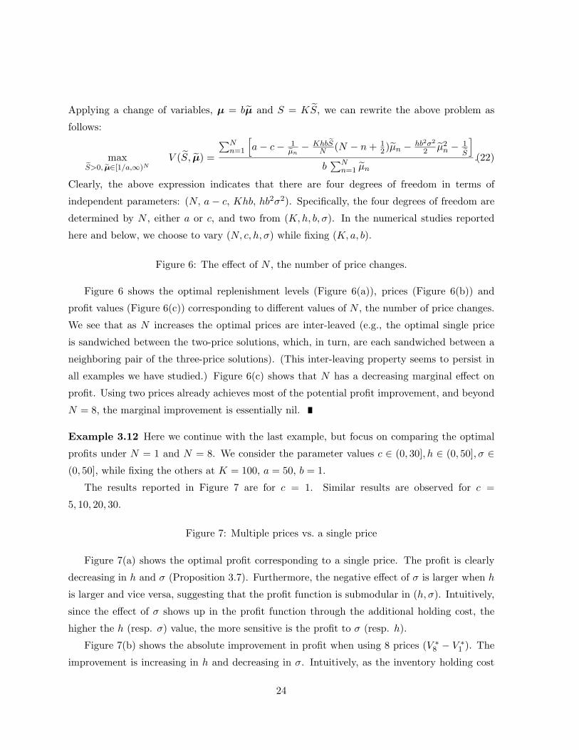
Figure 6: The effect of N , the number of price changes.

Figure 6 shows the optimal replenishment levels (Figure 6(a)), prices (Figure 6(b)) and

profit values (Figure 6(c)) corresponding to different values of N , the number of price changes.

We see that as N increases the optimal prices are inter-leaved (e.g., the optimal single price

is sandwiched between the two-price solutions, which, in turn, are each sandwiched between a

neighboring pair of the three-price solutions). (This inter-leaving property seems to persist in

all examples we have studied.) Figure 6(c) shows that N has a decreasing marginal effect on

profit. Using two prices already achieves most of the potential profit improvement, and beyond

N = 8, the marginal improvement is essentially nil.

Example 3.12 Here we continue with the last example, but focus on comparing the optimal

profits under N = 1 and N = 8. We consider the parameter values c ∈ (0, 30], h ∈ (0, 50], σ ∈(0, 50], while fixing the others at K = 100, a = 50, b = 1.

The results reported in Figure 7 are for c = 1. Similar results are observed for c =

5, 10, 20, 30.

Figure 7: Multiple prices vs. a single price

Figure 7(a) shows the optimal profit corresponding to a single price. The profit is clearly

decreasing in h and σ (Proposition 3.7). Furthermore, the negative effect of σ is larger when h

is larger and vice versa, suggesting that the profit function is submodular in (h, σ). Intuitively,

since the effect of σ shows up in the profit function through the additional holding cost, the

higher the h (resp. σ) value, the more sensitive is the profit to σ (resp. h).

Figure 7(b) shows the absolute improvement in profit when using 8 prices (V ∗8 − V ∗1 ). The

improvement is increasing in h and decreasing in σ. Intuitively, as the inventory holding cost

24

increases, the right trade-off among revenue, holding cost and replenishment cost becomes more

important, thus more pricing options over time is more beneficial. However, pricing becomes

less effective as demand variability (σ) increases.

Note that when the profit under a single price V ∗1 approaches zero, the absolute improvement

(V ∗8 −V ∗1 ) does not diminish. In particular, while V ∗1 decreases in h, the improvement increases

in h. Indeed, the relative improvement (= V ∗8 −V ∗

1V ∗1

) is increasing in h, and approaching infinity

when V ∗1 is close to zero, as demonstrated in Figure 7(c) and (d).

Figure 8: The bound on profit improvement

To conclude this example, we show in Figure 8 the profit improvement in comparison with

the heuristic bound in (21). The latter can be seen in this example as giving a good estimate

of the maximum potential improvement.

3.3.3 The Algorithm: Fractional Programming

To solve the fractional optimization problem in (20), we can instead solve the following:

maxS>0, µ∈MN

Vη :=N∑

n=1

[p( 1µn

)−hS(N − n+ 1

2)N

µn −hσ2

2µ2

n − a(S)

]− η

N∑n=1

µn, (23)

where η is a parameter such that when the optimal objective value of the problem in (23) is

zero, the corresponding solution is the optimal solution to the original problem in (20), and the

corresponding η is the optimal objective value of the original problem. To see the equivalence,

write the optimal value in (20) as V ∗ = A∗/B∗. Then, when η = V ∗, the optimal value of (23)

is zero. On the other hand, suppose there exists an η which yields a zero objective value in

(23), specifically, A∗ − ηB∗ = 0, then for any feasible A,B, we have A− ηB ≤ 0, which implies

A/B ≤ η = A∗/B∗.

The algorithm described below takes advantage of the separability of the objective function

with respect to µ when S and η are given. Specifically, the sub-problems are:

maxµn∈M

gn(µn) := p( 1µn

)−hS(N − n+ 1

2)N

µn −hσ2

2µ2

n − a(S)− ηµn, n = 1, . . . , N. (24)

Under Assumption 1, the objective in (24) is concave in µn.

Algorithm for solving (20)

1. Initialize η = η0, S = S0, and µn = µ for n = 1, . . . , N.(For instance, η0 = 0; S0 = S∗ and µn = µ∗ for all n,with (S∗, µ∗) being the optimal solution to the single-price problem.)Set ε and δ at small positive values (according to required precision).

25

2. Solve the N single-dimensional concave function maximization problems in (24).

3. Update S following a specified stepsize or use equation (9).If the difference between the new and the old S values is smaller than ε,go to step 4; otherwise, return to step 2.

4. If |Vη| ≤ ε, stop. Otherwise,if Vη > ε, increase η to η + δ;if Vη < −ε, decrease η to η − δ.Go to step 2.

In step 2, there are ways to accelerate the search procedure. Firstly, in searching the optimal

µ∗n for n = 1, . . . , N , we can take the advantage of the monotonicity of µ∗n in n following

Proposition 3.3. Secondly, we have gn(µ∗n) ≤ gn+1(µ∗n) ≤ gn+1(µ∗n+1), for n = 1, . . . , N − 1.

Hence, once we find µ∗1, if g1(µ∗1) > ε/N , then we can be sure that Vη > ε, and to bypass the

rest of the algorithm to increase η directly and proceed to the next loop. Thirdly, we can make

use of the monotonicity of µ∗n(S) in S according to Proposition 3.4 (iii). This is particularly

useful when the stepsize for updating S in step 3 is small.

In step 3, if we are in the early stage of the algorithm, i.e., when Vη is still substantially

away from zero, then the updating of S needs to cover a wide range so as not to miss the true

optimum. This can be done by using large stepsize first and then reduce them gradually. When

we are at the late stage of fine-tuning Vη, we can even bypass step 3 and simply use the same

S value (when it was last updated).

In step 3, we can use (9) as an updating scheme. This is in fact the coordinate assent method:

we alternate between optimizing µ for fixed S and optimizing S for fixed µ. This procedure

is guaranteed to converge to a local maximum, but not necessary the global maximum (see

Luenberger (1984)). So it is useful once the algorithm enters the region containing the true

optimum without other local maxima.

It can be verified that the optimal objective value in (23) is strictly decreasing in η, so there

is a unique zero-crossing point at which Vη is zero. Thus, in step 4, we can update η following

a standard line search algorithm, such as bi-section or the golden ratio.

4 Discounted Objective

We now turn to examining the problems in the last section under a discounted objective. We

will focus on the contrasts rather than the similarities between these two classes of models. So

as to present the results with minimal distraction, all proofs are relegated to the appendix.

26

Recall that period n refers to the period in which the price pn applies and the inventory

drops from Sn−1 = (N−n+1)SN to Sn = (N−n)S

N . Let γ > 0 be the discount rate. Let vn,γ(λn)

denote the expected profit over period n discounted to the beginning of the period. We have

vn,γ(λn) = E

[∫ τn

0e−γt

[p(λn)dD(t+ Tn−1)− hX(t+ Tn−1)dt

]]= E

[∫ τn

0e−γt

(p(λn) +

h

γ

)dD(t+ Tn−1) +

he−γτnSn

γ− hSn−1

γ

]=

(p(λn) +

h

γ

)λn

γ

(1− E[e−γτn ]

)+hE[e−γτn ]Sn

γ− hSn−1

γ

= f(λn) +hS(1−Θ(λn))

Nγn, (25)

where,

f(λ) =(p(λ) +

h

γ

)λγ

(1−Θ(λ)

)+hΘ(λ)S

γ− hS(N + 1)

Nγ,

Θ(λ) = E[e−γτn(λ)] = e−b(λ)S/N ,

b(λ) =

√λ2 + 2σ2γ − λ

σ2=

2γ√λ2 + 2σ2γ + λ

.

Here Lemma 2.1 is applied to derive the expression for Θ(λ). Assuming that the optimal λn is

finite, then Θ(λn) < 1. Let Vγ(S,λ) denote the discounted profit starting from zero inventory

under the policy (S,λ). Then,

Vγ(S,λ) =vγ(S,λ)

1−Θγ(S,λ), (26)

where,

vγ(S,λ) = v1,γ(λ1) + Θ(λ1)v2,γ(λ2) + · · ·+ Θ(λ1) . . .Θ(λN−1)vN,γ(λN )− c(S),

Θγ(S,λ) = Θ(λ1) . . .Θ(λN ) < 1.

For a single price, (26) becomes

Vγ(S, λ) =r(λ)γ− S(h/γ + a(S))

1− e−b(λ)S+hλ

γ2. (27)

Note in the above expressions vn,γ and Θ depend on S as well, but we have suppressed S to

simplify notation. For the same reason, we shall omit S in vγ(S,λ) and Θγ(S,λ) when S is not

a decision variable.

27

Optimal Replenishment

The problem is

maxS>0

Vγ(S, λ).

The first-order condition is

[h/γ + a(S) + Sa′(S)](ebS − 1) = bS[h/γ + a(S)]. (28)

Proposition 4.1 Vγ(S, λ) is concave in S if a′(S) < 0 and c′′(S) ≥ 0.

The condition a′(S) < 0 holds if S satisfies (28). Hence, the first-order condition in (28) is

sufficient for optimality if c′′(S) ≥ 0. We have also identified examples of multiple stationary

points when c′′(S) < 0.

Proposition 4.2 With price fixed,

(i) the optimal replenishment level S∗γ is increasing in σ, decreasing in h and p;

(ii) the optimal profit is decreasing in σ and h.

Recall, under the average objective and fixed price, the demand variability has no effect on

the optimal replenishment level. In contrast, the demand variability will raise the replenishment

level under the discounted objective. The following example further illustrates this point. Other

monotonicity properties in Proposition 3.1 continue to hold here.

Example 4.1 (EOQ under small discount rate) Suppose c(S) = K + cS. When γ is

small, b is also small, and the first order condition (28) can be approximately written as

(h/γ + c)(bS + 12b

2S2) = bS(h/γ +K/S + c).

Then,

S∗γ =

√2Kγ

b(h+ cγ).

Approximating b by Taylor series: b ≈ γλ −

σ2γ2

2λ3 , we have

S∗γ ≈

√2K(λ+ σ2γ

2λ )h+ cγ

.

Porteus (1985b) pointed out that the EOQ solution under a discounted objective can be ap-

proximated by√

2Kλh+cγ . Our result generalizes this result by incorporating the effect of demand

variability.

28

The Single-Price Problem

The problem is

maxλ∈L

Vγ(S, λ)

It is immediate to show that Vγ(S, λ) is concave in λ, and hence the optimal single price is

given by the first-order condition,

r′(λ) +hS + γc(S)

(1− e−b(λ)S)2Se−b(λ)Sb′(λ) +

h

γ= 0. (29)

Proposition 4.3 With the replenishment level fixed at S, let the optimal price be p∗. Then

(i) r′(λ(p∗)) ≤ a(S);

(ii) p∗ is decreasing in h;

(iii) p∗ is decreasing in S for S satisfying a′(S) ≤ 0;

(iv) the optimal profit is decreasing in σ and h.

Most results in Proposition 3.2 continue to hold here. The only difference is that the optimal

price is decreasing in demand variability under the average objective, while here the effect of

demand variability is rather unclear. Numerically, we have observed that in most cases the

optimal price is still decreasing in σ under the discounted objective, but exceptions do exist.

The pricing-replenishment joint optimization lacks the monotonicity properties of the opti-

mal decisions in general.

The N-Price Problem

The problem is

maxλ∈LN

Vγ(S,λ) (30)

This problem has an equivalent dynamic programming formulation. Let Vn,γ denote the optimal

discounted profit-to-go starting from the beginning of period n. Following the principle of

optimality, we have the following recursions:

V1,γ = maxλ∈L

{−c(S) + v1,γ(λ) + Θ(λ)V2,γ} ,Vn,γ = max

λ∈L{vn,γ(λ) + Θ(λ)Vn+1,γ} , n = 2, . . . , N − 1,

VN,γ = maxλ∈L

{vN,γ(λ) + Θ(λ)V1,γ} .(31)

The following parallels Proposition 3.3.

29

Proposition 4.4 For any fixed replenishment level S, the optimal prices under the discounted

objective are increasing over the periods, i.e., p∗1 ≤ p∗2 ≤ ... ≤ p∗N .

A Fixed-Point Algorithm

Instead of searching in LN for the optimal λ, we provide an iterative algorithm with each step

solving a one-dimensional problem in L.

A Fixed-Point Algorithm for the dynamic program (31)

1. Set an arbitrary initial value V o1,γ, and set ε > 0 small.

2. Use V o1,γ in the last equation of (31), and solve for VN,γ , VN−1,γ , . . . , V1,γ recursively

following (31).

3. If |V o1,γ − V1,γ | < ε, stop. Otherwise, let V o

1,γ ← V1,γ, and go to Step 2.

To explore the convergence of the algorithm, we substitute the equations for V2,γ , . . . , VN,γ

in (31) recursively into the first equation and obtain the following:

V1,γ = maxλ∈LN

{vγ(λ) + Θγ(λ)V1,γ

}≡ max

λ∈LNψ(λ, V1,γ) ≡ Ψ(V1,γ). (32)

Proposition 4.5 Let ψ and Ψ be defined as above, then

(i) the mapping Ψ(V ) is increasing and Lipschitz continuous with modulus 1;

(ii) there exists a unique fixed point satisfying V ∗ = Ψ(V ∗) = ψ(λ∗, V ∗). Furthermore, λ∗

solves (30) with the maximum discounted profit being V ∗; and

(iii) The above algorithm for solving (31) converges to the optimal solution from any initial

value V o1,γ.

Joint Pricing-Replenishment

In general, when N prices are optimized jointly with the replenishment level S, we can use

the iterative algorithm developed above for each fixed S, and then do a line search to find the

optimal S.

Convergence to the Average Objective

The discounted profit converges to the average profit in the following sense.

Proposition 4.6 Let vn,γ and Vγ be defined as (25) and (26), and let vn and V follow (6) and

(7) under the average objective. Then,

limγ→0

vn,γ = vn and limγ→0

γVγ = V.

30

As shown in the appendix, the first-order conditions in (28) and (29) converge to their

counterparts in (9) and (12), respectively. This implies that the optimal pricing-replenishment

decisions under the discounted objective converge to those under the average objective, notwith-

standing the contrasts highlighted above.

Proposition 4.7 Let (S∗γ , p∗γ) and (S∗, p∗) denote, respectively, the optimal solution under the

discounted and the average objectives. Then, we have

limγ→0

S∗γ = S∗ and limγ→0

p∗γ = p∗.

5 Concluding Remarks

We have demonstrated the effectiveness of the Brownian motion model for price-sensitive de-

mand, in particular in making optimal pricing and replenishment decisions, quantifying the

profit improvement, and bringing out the impact of demand variability. The Brownian mo-

tion model also enables us to work out explicit analytical solutions, which facilitate making

connections to and comparisons against, wherever applicable, previously known results in both

deterministic and stochastic settings.

Our models can be extended to allow backlogging, in which case the replenishment takes

the form of a (−s, S) policy: a replenishment order is issued whenever the backlog has reached

s, to bring the inventory level back to S. (Hence, the replenishment quantity is S + s. Assume

zero leadtime as before.) The pricing policy is modified accordingly: equally divide S and s

into N and M (positive integers) segments, respectively, such that

S = S0 > S1 > · · · > SN = 0 > SN+1 > · · · > SN+M = −s,

and apply price pn until the the net inventory (inventory on hand net the backlogs) falls to Sn,

n = 1, . . . , N +M .

Most of the results we have derived for the no-backlog case will continue to hold, with

suitable modifications. For instance, the optimal pricing will satisfy the monotonicity:

p∗1 ≤ p∗2 ≤ · · · ≤ p∗N , p∗N+1 ≥ p∗N+2 ≥ · · · ≥ p∗N+M .

That is, the optimal prices increase as the on-hand inventory is depleted, and decrease as the

backlog increases. The bound on the profit improvement is (assuming M = N):

V ∗N − V ∗1 ≤(1−N−2

)12

[hS2

µh

(σ2 + B

h

) +bs2

µb

(σ2 + B

b

)] ,31

where µh = 1N

∑Nn=1 µ

∗n, µb = 1

N

∑2Nn=N+1 µ

∗n, and B denotes, as before, the lower bound for

−d2p( 1

µ)

dµ2 over the spread of µ∗.

6 Appendix

Proof of Lemma 2.1. (This lemma follows from well-known results regarding optional

stopping applied to Brownian motion; refer to, e.g., Karlin and Taylor (1975), and Ross (1996).

The proof here is included for completeness.) Omit the subscript n, and write T := τn, x :=

T/N . We have

λT + σB(T ) = x. (33)

This, combined with EB(T ) = 0, which follows from applying optional stopping to B(t), leads

to (3).

To derive the second moment of T , we have

σ2[B2(T )− T ] = (x− λT )2 − σ2T.

Applying optional stopping again, to the martingale B2(t)− t, we have

E[(x− λT )2] = σ2E(T ),

which can be expressed as

λ2Var(T ) = σ2E(T ).

This establishes (4).

More generally, consider E(e−γT ), where γ > 0 is a constant (discount rate). Write

−γT = aB(T )− 12a2T − bx, (34)

where a and b are parameters to be determined. Then, applying optional stopping to the

exponential martingale, exp[aB(t)− 12a

2t], we have

E(e−γT ) = e−bx · E[eaB(T )− 12a2T ] = e−bx.

The power b can be derived as follows. Substituting (33) into the right hand side of (34), we

have

−γT = aB(T )− 12a2T − bσB(T )− bλT.

32

Equating the coefficients of T and B(T ) on both sides yields:

a = bσ,12a2 + bλ = r,

leading to

σa2 + 2λa− 2γσ = 0.

Hence,

a =

√λ2 + 2σ2γ − λ

σ;

and

E(e−γT ) = e−bx = exp[−√λ2 + 2σ2γ − λ

σ2x].

Proof of Lemma 3.1. First, assuming interior optimum. The first-order conditions in (15)

hold, which imply that

dvm(µm)dµm

=dvn(µn)dµn

,

or equivalently,

dpdµ( 1

µ∗m)− dp

dµ( 1µ∗n

) + hSN (m− n) + hσ2(µ∗n − µ∗m) = 0. (35)

By Proposition 3.3, µ∗n ≥ µ∗m for n > m. Next, applying the mean-value theorem and using the

definition of B, we have

dpdµ( 1

µ∗m)− dp

dµ( 1µ∗n

) = − d2pdµ2 (1

ζ )(µ∗n − µ∗m) ≥ B(µ∗n − µ∗m), (36)

where ζ ∈ [µ∗m, µ∗n]. Combining (35) and (36), we have

hSN (m− n) + (hσ2 +B)(µ∗n − µ∗m) ≤ 0,

or

µ∗n − µ∗m ≤ S(n−m)N(σ2 + B

h

) .Next, we show the above result holds even when the optimum is on the boundary. If

µ∗m = µ∗n, then the desired inequality obviously holds. If µ∗m < µ∗n, consider the following

33

alternative pricing policy: (µ∗1, . . . , µ∗m + δ, . . . , µ∗n − δ, . . . , µ∗N ), where 0 < δ < µ∗n−µ∗m

2 . Since

this alternative cannot be better than the optimum, we have

p( 1µ∗m+δ ) + p( 1

µ∗n−δ )− hSN

[(N −m+ 1

2)(µ∗m + δ) + (N − n+ 12)(µ∗n − δ)

]−hσ2

2

[(µ∗m + δ)2 + (µ∗n − δ)2

]≤ p( 1

µ∗m) + p( 1

µ∗n)− hS

N

[(N −m+ 1

2)µ∗m + (N − n+ 12)µ∗n

]− hσ2

2

[µ∗2m + µ∗2n

].

Taylor’s expansion with straightforward algebra simplifies the inequality to

dpdµ( 1

µ∗m+ζ1δ )δ − dpdµ( 1

µ∗n−ζ2δ )δ + hSN δ(m− n) + hσ2δ(µ∗n − µ∗m − δ) ≤ 0,

where ζ1, ζ2 ∈ [0, 1]. Dividing both sides by δ, and then letting δ → 0, we have

dpdµ( 1

µ∗m)− dp

dµ( 1µ∗n

) + hSN (m− n) + hσ2(µ∗n − µ∗m) ≤ 0. (37)

Combining (36) and (37) yields the desired inequality.

Proof of Lemma 3.2. We only prove part (i); the proof of part (ii) and (iii) is completely

analogous. Consider an equivalent problem to the fractional problem (13):

maxµ

N∑n=1

[p( 1µn

)−hS(N − n+ 1

2)N

µn −hσ2

2µ2

n − a(S)

]− η(σ)

N∑n=1

µn,

where η(σ) is the optimal value of (13) when the demand variability is σ and all the other

parameters are fixed. To solve the above problem, we can maximize each µn separately:

maxµn

gn(µn, σ) = p( 1µn

)−hS(N − n+ 1

2)N

µn −hσ2

2µ2

n − η(σ)µn.

Since µ∗(σ) is in the interior, applying the envelope theorem, we have

dη

dσ= −

hσ∑N

k=1 µ∗k2∑N

k=1 µ∗k

.

To establish the desired monotonicity, it suffices to establish the submodularity of gn(µn, σ)

(refer to Topkis 1978):

∂2gn(µ∗n, σ)∂µn∂σ

= −2hσµ∗n −∂η

∂σ

= −2hσµ∗n +hσ∑N

k=1 µ∗k2∑N

k=1 µ∗k

.

=hσ∑Nk=1 µ

∗k

(N∑

k=1

µ∗k2 − 2µ∗n

N∑k=1

µ∗k

),

34

If∑µ∗k

2−2µ∗n∑µ∗k < 0, then the objective gn(µn, σ) is submodular in (µn, σ) in a neighborhood

of (µ∗n, σ). Thus, µ∗n is (locally) decreasing in σ. If the converse is true, µ∗n is (locally) increasing

in σ.

Proof of Proposition 4.1. Recall

Vγ(S, λ) =r(λ)γ− S(h/γ + a(S))

1− e−b(λ)S+hλ

γ2.

We first show that Vγ(S, λ) is concave in S if a′(S) ≤ 0 and c′′(S) ≥ 0. To this end, we derive

∂2Vγ

∂S2= −

(bSe−bS + 2e−bS + bS − 2)e−bSb(hγ + a(S))

(1− e−bS)3+

2bSe−bSa′(S)(1− e−bS)2

− c′′(S)1− e−bS

.

The first term on the right side is negative due to the fact that

h(x) := xe−x + 2e−x + x− 2 ≥ 0 for all x ≥ 0, (38)

since h(0) = h′(0) = 0 and h′′(x) = xe−x ≥ 0 for all x ≥ 0; the second term is negative since

a′(S) ≤ 0; the third term is also negative if c(S) is convex in S. Hence Vγ(S, λ) is concave in S

if a′(S) ≤ 0 and c′′(S) ≥ 0.

To show Vγ is concave in λ, it suffices to show that g(λ) := 11−e−b(λ)S is convex in λ. We

have,

g′′(λ) = g2e−bSS(b′

2S(2ge−bS + 1)− b′′

)=

g2e−bSS

λ2 + 2γσ2

(b2S(2ge−bS + 1)− 2γ√

λ2 + 2γσ2

),

where the last equality follows from b′ = − b√λ2+2γσ2

and b′′ = 2γ(λ2+2γσ2)3/2 . Since

b2S(2ge−bS + 1)− 2γ√λ2 + 2γσ2

> b2S(2ge−bS + 1)− 2b

= bg(bSe−bS + bS + 2e−bS − 2)

≥ 0,

where the last inequality is again due to (38), g(λ) is convex in λ, and hence, Vγ(S, λ) is concave

in λ.

Proof of Proposition 4.2.

35

(i). To show that S∗ is decreasing in p, it suffices to verify that Vγ(S, λ) is supermodular in

(S, λ); i.e., ∂2V∂S∂λ ≥ 0. Since the optimal replenishment level must satisfy a′(S) < 0 by (i), it

suffices to verify the supermodularity in the sub-lattice where a′(S) < 0.

We have

∂2Vγ(S, λ)∂S∂λ

= g2e−bSb′S[hγ

+ c′(S)−(hγ

+ a(S))(bS

1 + e−bS

1− e−bS− 1)].

Since b′(λ) < 0, and since a′(S) < 0 is equivalent to c′(S) < a(S), the desired ∂2Vγ

∂S∂λ ≥ 0 is

implied by

bS1 + e−bS

1− e−bS− 1 ≥ 1.

But this last inequality follows immediately from (38).

The proof of S∗ increasing in σ is completely analogous: we can follow the above to establish∂2Vγ

∂S∂σ ≥ 0 in the sub-lattice where a′(S) < 0; the only change is to replace b′(λ) by b′(σ). Note

in particular that b′(σ) < 0 too.

To show that S∗ is decreasing in h, note that Vγ is submodular in (S, h):

∂2Vγ

∂S∂h= −1− e−bS − bSe−bS

γ(1− e−bS)2≤ 0,

since 1− e−bS ≥ bSe−bS .

(ii). The proof is analogous to the proof of Proposition 3.1 (ii).

Proof of Proposition 4.3.

(i). From (29),

r′(λ) =hS + a(S)Sγ(1− e−bS)2

Se−bS(−b′)− h

γ

= a(S)e−bSS2γ

(1− e−bS)2b√

λ2 + 2σ2γ+

h√λ2 + 2σ2γ

bS2e−bS

(1− e−bS)2− h

γ

= a(S)e−bSS2b2

(1− e−bS)21

2− λγ b

+h

b√λ2 + 2σ2γ

(b2S2e−bS

(1− e−bS)2− b√λ2 + 2σ2γ

γ

)

≤ a(S)2− λ

γ b+

h

b√λ2 + 2σ2γ

(1− b

√λ2 + 2σ2γ

γ

)≤ a(S),

36

where the first inequality results from the following:

x2e−x

(1− e−x)2=

x2

ex + e−x − 2=

x2∑∞n=1 2x2n/(2n)!

≤ 1, (39)

and in the last inequality we used the fact that

γ√λ2 + 2σ2γ

≤ b =2γ√

λ2 + 2σ2γ + λ≤ γ

λ. (40)

(ii) To prove the monotonicity in h, we show that Vγ is supermodular in (λ, h):

∂2V

∂λ∂h=

S2e−bSb′

γ(1− e−bS)2+

1γ2

=1bγ2

[− e−bSS2b2

(1− e−bS)2γ√

λ2 + 2σ2γ+ b

]

≥ 1bγ2

[− γ√

λ2 + 2σ2γ+ b

]≥ 0,

where the first inequality follows from (39) and the last inequality follows from (40).

(iii) The monotonicity in S relies on the supermodularity of Vγ in (S, λ), which has been

established in the proof of Proposition 4.2 (ii).

(iv). The proof is analogous to the proof of Proposition 3.1 (iii).

Proof of Proposition 4.4. Let the optimal profit-to-go be V ∗n,γ , for n = 1, . . . , N , which

satisfy (32). For simplicity, denote V ∗N+1,γ := V1,γ . In view of (32) and (25), we can write

λ∗n ∈ arg maxλ∈L

{F (n, λ)}, for n = 1, . . . , N,

where

F (n, λ) = f(λ) +hS(1−Θ(λ))

Nγn+ Θ(λ)V ∗n+1,γ .

Thus, λ∗n is decreasing in n if we can show that F (n, λ) is submodular in (n, λ). To this end,

notice that

F (n, λ)− F (n− 1, λ) =hS(1−Θ(λ))

Nγ+ Θ(λ)(V ∗n+1,γ − V ∗n,γ)

=hS

Nγ+ Θ(λ)

(V ∗n+1,γ − V ∗n,γ −

hS

Nγ

), for n = 2, . . . , N.

37

Since Θ(λ) is decreasing in λ, the above difference is decreasing in λ if V ∗n+1,γ−V ∗n,γ ≥ hSNγ . This

last inequality can be verified as follows. For n = 2, . . . , N , if we start from the inventory levelS(N−n+1)

N , then the optimal profit-to-go is V ∗n,γ . Now consider the following strategy: always

keep SN units in stock while following the optimal policy as if the inventory starts at S(N−n)

N .

The profit associated with this strategy is V ∗n+1,γ − hSNγ , where hS

Nγ is the discounted cost of

holding the extra SN units. Since this strategy is sub-optimal, we have

V ∗n+1,γ − V ∗n,γ ≥ V ∗n+1,γ −(V ∗n+1,γ −

hS

Nγ

)=

hS

Nγ.

The submodularity of F (n, p) hence follows and λ∗n is decreasing in n; or equivalently, p∗n is

increasing in n.

Proof of Proposition 4.5.

(i). For V > V , let λ and λ be the maximizers (not necessarily in the interior) of ψ(·, V ) and

ψ(λ, V ), respectively (refer to (32)). Then,

Ψ(V )−Ψ(V ) = ψ(λ, V )− ψ(λ, V ) ≥ ψ(λ, V )− ψ(λ, V ) = Θγ(λ)(V − V ) ≥ 0,

which implies that Ψ(V ) is increasing in V . Furthermore,

Ψ(V )−Ψ(V ) = ψ(λ, V )− ψ(λ, V ) ≤ ψ(λ, V )− ψ(λ, V ) = Θγ(λ)(V − V ). (41)

Since Θγ(λ) ≤ 1, the above inequality implies that Ψ is Lipschitz continuous, with modulus no

larger than 1. That is, Ψ(V ) is non-expansive.

(ii). Let λ∗ be the optimal solution to (30) with optimal value V ∗. We eliminate the un-

interesting case where λ∗ = ∞. Thus, Θγ(λ∗) < 1 and V ∗ = vγ(λ∗)1−Θγ(λ∗) , or equivalently,

V ∗ = ψ(λ∗, V ∗). On the other hand, V ∗ ≥ vγ(λ)1−Θγ(λ) , or equivalently, V ∗ ≥ ψ(λ, V ∗) for all

λ ∈ LN . Thus, V ∗ = maxλ∈LN ψ(λ, V ∗) = Ψ(V ∗); and hence, V ∗ is a fixed point of Ψ. This

proves the existence.

Conversely, suppose V ∗ is a fixed point of Ψ(V ) with the corresponding maximizer λ∗. Note

that λ∗ =∞ implies that all inventory can be sold out instantaneously after the replenishment

(with the revenue covering exactly the replenishment cost). If we eliminate this uninteresting

case, then Θγ(λ∗) < 1, and V ∗ = ψ(λ∗, V ∗) or V ∗ = vγ(λ∗)1−Θγ(λ∗) . At the same time, V ∗ ≥ ψ(λ, V ∗)

or V ∗ ≥ vγ(λ)1−Θγ(λ) for all λ ∈ LN . Hence, λ∗ solves the problem in (30), achieving the optimal

value V ∗.

38

Now, suppose there exist two fixed points V ∗ > V ∗ corresponding to the maximizers λ∗ and

λ∗, respectively. Then, both V ∗ and V ∗ are optimal values for the problem in (30), an obvious

contradiction (against optimality). This establishes the uniqueness.

(iii). Let V ∗ be the unique fixed point. From (i), we have Ψ(V ) > V for V < V ∗ and Ψ(V ) < V

for V > V ∗. Hence, if we start from an initial value V0 < V ∗, the sequence of values generated

by the iteration Vn = Ψ(Vn−1) is increasing and bounded from above by V ∗. So the sequence

converges to a fixed point of the mapping Ψ, which must be V ∗. A similar argument holds for

an initial value V0 > V ∗.

Proof of Proposition 4.6. When γ → 0, via Taylor expansion, we can derive the following:

b(λ) =γ

λ− σ2γ2

2λ3+O(γ3), (42)

Θ(λ) = e−b(λ)S/N = 1− Sγ

Nλ+σ2Sγ2

2Nλ3+

S2γ2

2N2λ2+O(γ3). (43)

Applying (42) and (43), we have

vn,γ(λ) =(p(λ) +

h

γ

)( SN− σ2Sγ

2Nλ2− S2γ

2N2λ

)+hS

γ− hS2

Nλ− hS(N + 1)

Nγ+hS2n

N2λ+ o(1)

=p(λ)SN

−hS2(N − n+ 1

2)N2λ

− hσ2S

2Nλ2+ o(1)

= vn(λ) + o(1), as γ → 0.

Then,

γVγ(S,λ) =vγ(λ)

γ−1(1−Θγ(λ))=

∑n vn(λn)− c(S) + o(1)

γ−1(1−∏N

n=1(1−Sγ

Nλn))

=∑

n vn(λn)− c(S) + o(1)SN

∑n λ

−1n + o(1)

= V (S,µ) + o(1), as γ → 0.

Proof of Proposition 4.7. The first-order optimality equation for S∗γ in (28) can be written

as follows:

(h+ γc′(S))(Sγ

λ− σ2Sγ2

2λ3− S2γ2

2λ2) = (1− Sγ

λ)(γ

λ− σ2γ2

2λ3)[hS + γc(S)]

Ignoring higher-order terms, we can simplify the above to the equation in (9), which is the

first-order optimality condition for S∗.

39

Using (42) and (43), when γ → 0, the first-order condition in (29) can be approximated as

0 = r′(λ) +(h+ γa(S))S

S2γ2

λ2 (1− σ2γ2λ2 − Sγ

2λ )2S(1− Sγ

λ

)(− γ

λ2+

3σ2γ2

2λ4

)+h

γ

= r′(λ)−(hγ

+ a(S))(

1 +σ2γ

λ2+Sγ

λ

)(1− Sγ

λ

)(1− 3σ2γ

2λ2

)+h

γ

= r′(λ)− h

γ− a(S)− h

γ

(σ2γ

λ2+Sγ

λ− Sγ

λ− 3σ2γ

2λ2

)+h

γ

= r′(λ)− a(S) +hσ2

2λ2,

which is exactly the same as the first-order condition in (12) for the average objective.

References

[1] Chen, F.Y., S. Ray, and Y. Song. 2003. Optimal pricing and inventory control policy in

periodic-review systems with fixed ordering cost and lost sales. Working paper, Chinese

University of Hong Kong.

[2] Chen, H. and D.D. Yao. 2001. Fundamentals of Queueing Networks: Performance, Asymp-

totics and Optimization, Springer-Verlag, New York.

[3] Chen, X. and D. Simchi-Levi. 2003a. Coordinating inventory control and pricing strategies

with random demand and fixed ordering cost: the finite horizon case. Operations Research,

forthcoming.

[4] Chen, X. and D. Simchi-Levi. 2003b. Coordinating inventory control and pricing strategies

with random demand and fixed ordering cost: the infinite horizon case. Working paper,

M.I.T.

[5] Chen, X. and D. Simchi-Levi. 2003c. Coordinating inventory control and pricing strategies

with random demand and fixed ordering cost: the continuous review model. Working paper,

M.I.T.

[6] Csorgo, M. and L. Horvath. 1993. Weighted Approximations in Probability and Statistics,

Wiley, New York.

[7] Elmaghraby W. and P. Keskinocak. 2003. Dynamic pricing in the presence of inventory

considerations: research overview, current practices and future directions. Management

Science, 49 (10), 1287-1309.

40

[8] Federgruen, A. and A. Heching. 1999. Combined pricing and inventory control under un-

certainty. Operations Research, 47 (3), 454-475.

[9] Feng, Y. and F.Y. Chen. 2002. Joint pricing and inventory control with setup costs and

demand uncertainty. Working paper, Chinese University of Hong Kong.

[10] Feng, Y. and F.Y. Chen. 2003. Pricing and inventory control for a periodic-review system:

optimality and optimization of (s, S, p) policy. Working paper, Chinese University of Hong

Kong.

[11] Harrison, J.M. 1985. Brownian Motion and Stochastic Flow Systems, Wiley, New York.

[12] Harrison, J.M. 1988. Brownian models of queueing networks with heterogeneous customer

populations. In: Stochastic Differential Systems, Stochastic Control Theory and Applica-

tions, IMA Volumes in Mathematics and its Applications, volume 10, W. Flemming and

P.L. Lions (eds.), 147-186, Springer-Verlag, New York.

[13] Harrison, J.M. 2003. A broader view of Brownian networks. Annals of Applied Probability,

13 (3), 1119-1150.

[14] Karlin, S. and H. Taylor 1975. A First Course in Stochastic Processes (2nd ed.), Academic

Press, New York.

[15] Li, L. 1988. A stochastic theory of the firm. Mathematics of Operations Research, 13 (3),

447-466.

[16] Luenberger, D.G. 1984. Linear and Nonlinear Programming (2nd ed.), Addison-Wesley.

[17] Mangasarian O.L. 1970. Convexity, pseudo-convexity and quasi-convexity of composite

functions. Cahiers du Centre d’Etudes de Recherche Operationnelle, 12, 114-122.

[18] Polatoglu, H. and I. Sahin. 2000. Optimal procurement policies under price-dependent

demand. International Journal of Production Economics, 65, 141-171.

[19] Porteus, E.L. 1985a. Investing in reduced setups in the EOQ model. Management Science,

31 (8), 998-1010.

[20] Porteus, E.L. 1985b. Undiscounted approximations of discounted regenerative models. Op-

erations Research Letters, 3, 293-300.

41

[21] Puterman, M.L. 1975. A diffusion process model for a storage system. In Logistics, M.A.

Geisler (ed.), North-Holland Publishing Company, 143-159.

[22] Rajan, A., Rakesh Steinberg and Richard Steinberg. 1992. Dynamic pricing and ordering

decisions by a monopolist. Management Science, 38 (2), 240-262.

[23] Ross, S.M. 1996. Stochastic Processes (2nd ed.) Wiley, New York.

[24] Thomas, L.J. 1974. Price and production decisions with random demand. Operations Re-

search, 22 (3), 513-518.

[25] Thowsen, G.T. 1975. A dynamic, nonstationary invneotry problem for a price/quantity

setting firm. Navel Research Logistics Quaterly, 22, 461-476.

[26] Topkis, D.M. 1978. Minimizing a submodular function on a lattice. Operations Research,

26 (2), 305-321.

[27] Whitin, T.M. 1955. Inventory control and price theory. Management Science, 2 (1), 61-68.

[28] Yano, C.A. and S.M. Gilbert. 2003. Coordinated pricing and production/procurement deci-

sions: a review. In: Managing Business Interfaces: Marketing, Engineering and Manufac-

turing Perspectives, A. Chakravarty and J. Eliashberg (eds.), Kluwer Academic Publishers

(forthcoming).

[29] Zabel E. 1972. Multiperiod monopoly under uncertainty. Journal of Economic Theory, 5,

524-536.

42

1

10 20 30 40p0

20

40

60

80

S

(a)

10 20 30 40p

200

100

0

100

200

300

400

V

σσσσ 1111

σσσσ 30303030

σσσσ 60606060

(b)

Figure 1. Optimal replenishment with a fixed price

2

20 40 60 80 100S25

30

35

p

σσσσ 1111σσσσ 30303030σσσσ 60606060

(a)

20 40 60 80 100S0

100

200

300

400

500V

σσσσ 1111σσσσ 30303030σσσσ 60606060

(b)

Figure 2. Optimal price with a fixed replenishment level

3

5 10 15 200

10

20

30

40

50

p

p1

p2

p3

p4

(a) The highest price is decreasing in σ

0.5 1 1.5 2 2.5 30

10

20

30

40

50

p

p1

p2

p3

p4

(b) The lowest price is decreasing in h

100 200 300 400

24

26

28

30

p

p1

p2

p3

p4

(c) The lowest price is decreasing in S

Figure 3. Optimal N prices and optimal single price

σ

h

S

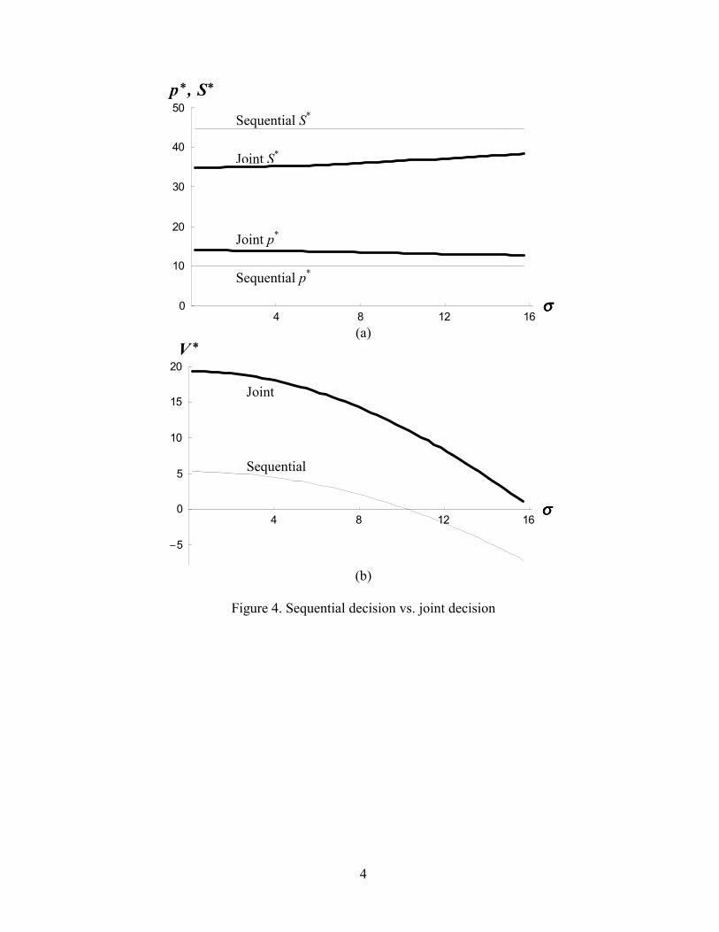
0

10

20

30

40

50p, S

5

0

5

10

15

20V

Sequential S*

Joint p*

4 8 12 16σσσσ

(a)

F

Sequential p*

Joint

Joint S*

4

4 8 12 16σσσσ

(b)

igure 4. Sequential decision vs. joint decision

Sequential

5

0.24 0.242 0.244 0.246 0.248 0.250

2

4

6

8

0.24 0.242 0.244 0.246 0.248 0.2541

41.5

42

42.5

43

0.24 0.242 0.244 0.246 0.248 0.254.2

4.4

4.6

4.8

5

Figure 5. Impact of demand variability on optimal solutions

µ1*

S*

µ2*

σ

σ

σ

6

1 2 3 4 5 6 7 8 1066

66.1

66.2

66.3

66.4

S

(a)

1 2 3 4 5 6 7 8 10

27.5

28

28.5

29p

(b)

1 2 3 4 5 6 7 8 10437.4

437.5

437.6

V

(c)

Figure 6. The effect of N, the number of price changes

50

50

50

N

N

N

7

010

2030

4050

h0

10

20

30

40

50

0

200

400

010

2030

4050

h

(a)

010

2030

4050

h0

10

20

30

40

50

0

2.5

5

7.5

10

010

2030

4050

h

(b)

h

σσσσ

h

σσσσ

8

010

2030

4050

h0

10

20

30

40

50

0

2.5

5

7.5

10

010

2030

4050

h

(c)

0 10 20 30 40 50

h

0

10

20

30

40

50

00.000250.00050.000750.001

(d)

Figure 7. Multiple prices vs. a single price

h

σσσσ

σσσσ

h

1% 2% 3% 4% 5% 8%

20%

(%)

9

1020

3040h

0

5

10

15

1020

3040h

Figure 8. The bound on profi

h

Bound

50

10

20

30

40

50

50

t improvement

σσσσ