Optimal Prediction for Radiative Transfer: A New … Prediction for Radiative Transfer: A New Perspective on Moment Closure Benjamin Seibold MIT Applied Mathematics Mar 02nd, 2009

Optimal Prediction for Radiative Transfer:A New Perspective on Moment Closure

Benjamin SeiboldMIT Applied Mathematics

Mar 02nd, 2009

Collaborator

Martin Frank (TU Kaiserslautern)

Partial Support

NSF DMS-0813648

Benjamin Seibold (MIT) A New Perspective on Moment Closure 03/02/2009, College Park 1 / 26

Overview

1 Moment Models for Radiative Transfer

2 Optimal Prediction

3 A New Perspective on Moment Closure in Radiative Transfer


Moment Models for Radiative Transfer

Overview





Moment Models for Radiative Transfer Equations and approaches

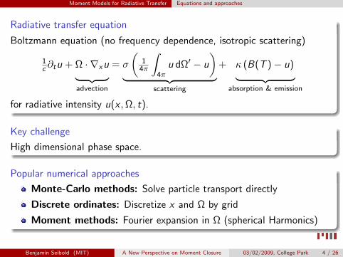
Radiative transfer equation

Boltzmann equation (no frequency dependence, isotropic scattering)

1c ∂tu + Ω · ∇xu︸︷︷︸

advection

= σ

(1

4π

∫4π

u dΩ′ − u

)︸︷︷︸

scattering

+ κ (B(T )− u)︸︷︷︸absorption & emission

for radiative intensity u(x ,Ω, t).

Key challenge

High dimensional phase space.

Popular numerical approaches

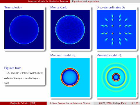
Monte-Carlo methods: Solve particle transport directly

Discrete ordinates: Discretize x and Ω by grid

Moment methods: Fourier expansion in Ω (spherical Harmonics)


Moment Models for Radiative Transfer Equations and approaches

True solution Monte Carlo Discrete ordinates S6

Figures from

T. A. Brunner, Forms of approximate

radiation transport, Sandia Report,

2002

Moment model P1 Moment model P5


Moment Models for Radiative Transfer Moment models

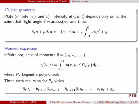
1D slab geometry

Plate (infinite in y and z). Intensity u(x , µ, t) depends only on x , theazimuthal flight angle θ = arccos(µ), and time.

∂tu + µ∂xu = −(κ+σ)u + σ2

∫ 1

−1u dµ′ + q

Moment expansion

Infinite sequence of moments ~u = (u0, u1, . . . )

uk (x , t) =

∫ 1

−1u(x , µ, t)Pk (µ) dµ ,

where Pk Legendre polynomials.

Three term recursion for Pk yields

∂tuk + bk,k−1∂xuk−1 + bk,k+1∂xuk+1 = −ckuk + qk .



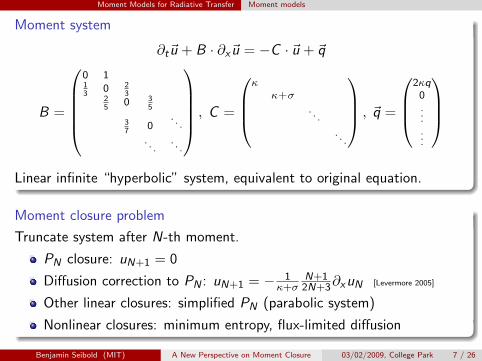
Moment system

∂t~u + B · ∂x~u = −C · ~u + ~q

B =

0 113

0 23

25

0 35

37

0. . .

. . .. . .

, C =

κ

κ+σ

. . .

. . .

, ~q =

2κq

0......

Linear infinite “hyperbolic” system, equivalent to original equation.

Moment closure problem

Truncate system after N-th moment.

PN closure: uN+1 = 0

Diffusion correction to PN : uN+1 = − 1κ+σ

N+12N+3∂xuN [Levermore 2005]

Other linear closures: simplified PN (parabolic system)

Nonlinear closures: minimum entropy, flux-limited diffusion



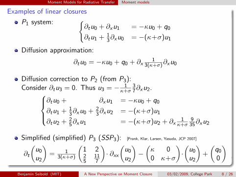
Examples of linear closures

P1 system: ∂tu0 + ∂xu1 = −κu0 + q0

∂tu1 + 13∂xu0 = −(κ+σ)u1

Diffusion approximation:

∂tu0 = −κu0 + q0 + ∂x1

3(κ+σ)∂xu0

Diffusion correction to P2 (from P3):Consider ∂tu3 = 0. Thus u3 = − 1

κ+σ37∂xu2.

∂tu0 + ∂xu1 = −κu0 + q0

∂tu1 + 13∂xu0 + 2

3∂xu2 = −(κ+σ)u1

∂tu2 + 25∂xu1 = −(κ+σ)u2 + ∂x

1κ+σ

935∂xu2

Simplified (simplified) P3 (SSP3): [Frank, Klar, Larsen, Yasuda, JCP 2007]

∂t

(u0

u2

)= 1

3(κ+σ)

(1 225

117

)· ∂xx

(u0

u2

)−(κ 00 κ+σ

)·(

u0

u2

)+

(q0

0

)Benjamin Seibold (MIT) A New Perspective on Moment Closure 03/02/2009, College Park 8 / 26


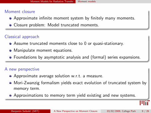
Moment closure

Approximate infinite moment system by finitely many moments.

Closure problem: Model truncated moments.

Classical approach

Assume truncated moments close to 0 or quasi-stationary.

Manipulate moment equations.

Foundations by asymptotic analysis and (formal) series expansions.

A new perspective

Approximate average solution w.r.t. a measure.

Mori-Zwanzig formalism yields exact evolution of truncated system bymemory term.

Approximations to memory term yield existing and new systems.


Optimal Prediction

Overview





Optimal Prediction

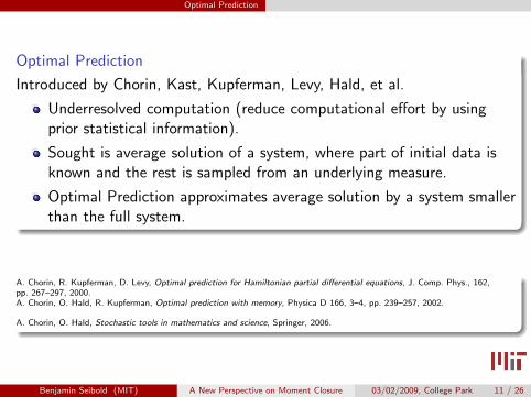
Optimal Prediction

Introduced by Chorin, Kast, Kupferman, Levy, Hald, et al.

Underresolved computation (reduce computational effort by usingprior statistical information).

Sought is average solution of a system, where part of initial data isknown and the rest is sampled from an underlying measure.

Optimal Prediction approximates average solution by a system smallerthan the full system.

A. Chorin, R. Kupferman, D. Levy, Optimal prediction for Hamiltonian partial differential equations, J. Comp. Phys., 162,pp. 267–297, 2000.A. Chorin, O. Hald, R. Kupferman, Optimal prediction with memory, Physica D 166, 3–4, pp. 239–257, 2002.

A. Chorin, O. Hald, Stochastic tools in mathematics and science, Springer, 2006.


Optimal Prediction

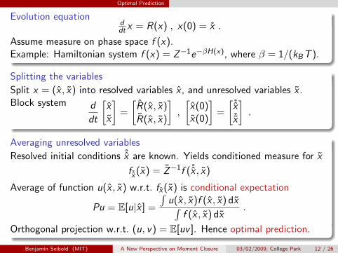
Evolution equationddt x = R(x) , x(0) = x .

Assume measure on phase space f (x).Example: Hamiltonian system f (x) = Z−1e−βH(x), where β = 1/(kBT ).

Splitting the variables

Split x = (x , x) into resolved variables x , and unresolved variables x .Block system d

dt

[xx

]=

[R(x , x)

R(x , x)

],

[x(0)x(0)

]=

[˚x˚x

].

Averaging unresolved variables

Resolved initial conditions ˚x are known. Yields conditioned measure for x

fx (x) = Z−1f (˚x , x)

Average of function u(x , x) w.r.t. fx (x) is conditional expectation

Pu = E[u|x ] =

∫u(x , x)f (x , x) dx∫

f (x , x) dx.

Orthogonal projection w.r.t. (u, v) = E[uv ]. Hence optimal prediction.


Optimal Prediction Ensemble average solution in weather forecast

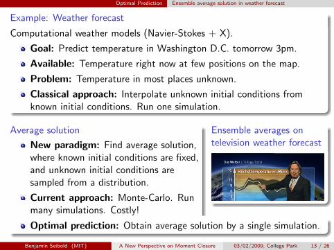
Example: Weather forecast

Computational weather models (Navier-Stokes + X).

Goal: Predict temperature in Washington D.C. tomorrow 3pm.

Available: Temperature right now at few positions on the map.

Problem: Temperature in most places unknown.

Classical approach: Interpolate unknown initial conditions fromknown initial conditions. Run one simulation.

Average solution

New paradigm: Find average solution,where known initial conditions are fixed,and unknown initial conditions aresampled from a distribution.

Current approach: Monte-Carlo. Runmany simulations. Costly!

Ensemble averages ontelevision weather forecast

Optimal prediction: Obtain average solution by a single simulation.


Optimal Prediction Ensemble average solution in weather forecast

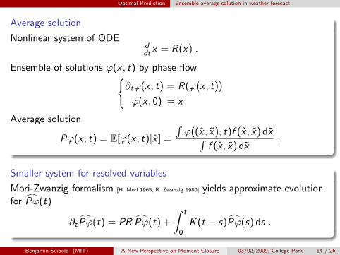
Average solution

Nonlinear system of ODEddt x = R(x) .

Ensemble of solutions ϕ(x , t) by phase flow∂tϕ(x , t) = R(ϕ(x , t))

ϕ(x , 0) = x

Average solution

Pϕ(x , t) = E[ϕ(x , t)|x ] =

∫ϕ((x , x), t)f (x , x) dx∫

f (x , x) dx.

Smaller system for resolved variables

Mori-Zwanzig formalism [H. Mori 1965, R. Zwanzig 1980] yields approximate evolutionfor Pϕ(t)

∂t Pϕ(t) = PR Pϕ(t) +

∫ t

0K (t − s)Pϕ(s) ds .


Optimal Prediction Types and Examples

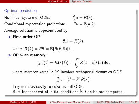
Optimal prediction

Nonlinear system of ODE: ddt x = R(x).

Conditional expectation projection: Pu = E[u|x ].

Average solution is approximated by

First order OP:ddt x = R(x) ,

where R(x) = PR = E[R(x , x)|x ].

OP with memory:

ddt x(t) = R(x(t)) +

∫ t

0K (t − s)x(s) ds ,

where memory kernel K (t) involves orthogonal dynamics ODE

ddt x = (I − P)R(x) .

In general as costly to solve as full ODE.But: Independent of initial conditions ˚x . Can be pre-computed.


A New Perspective on Moment Closure in Radiative Transfer

Overview





A New Perspective on Moment Closure in Radiative Transfer

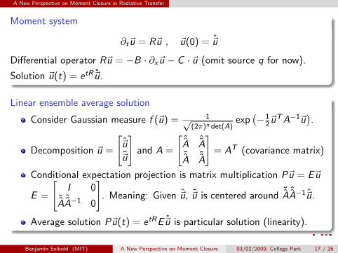
Moment system

∂t~u = R~u , ~u(0) = ~u

Differential operator R~u = −B · ∂x~u − C · ~u (omit source q for now).

Solution ~u(t) = etR~u.

Linear ensemble average solution

Consider Gaussian measure f (~u) = 1√(2π)n det(A)

exp(−1

2~uT A−1~u

).

Decomposition ~u =

[~u

~u

]and A =

[Â ÂÃ Ã

]= AT (covariance matrix)

Conditional expectation projection is matrix multiplication P~u = E~u

E =

[I 0

Ã Â−1 0

]. Meaning: Given ~u, ~u is centered around Ã Â−1~u.

Average solution P~u(t) = etRE~u is particular solution (linearity).


A New Perspective on Moment Closure in Radiative Transfer Linear optimal prediction

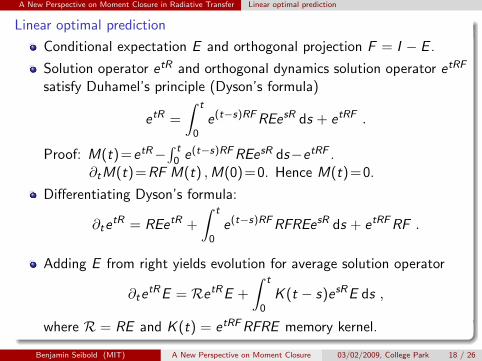
Linear optimal prediction

Conditional expectation E and orthogonal projection F = I − E .

Solution operator etR and orthogonal dynamics solution operator etRF

satisfy Duhamel’s principle (Dyson’s formula)

etR =

∫ t

0e(t−s)RF REesR ds + etRF .

Proof: M(t)=etR−∫ t

0 e(t−s)RF REesR ds−etRF .∂tM(t)=RF M(t) ,M(0)=0. Hence M(t)=0.

Differentiating Dyson’s formula:

∂tetR = REetR +

∫ t

0e(t−s)RF RFREesR ds + etRF RF .

Adding E from right yields evolution for average solution operator

∂tetRE = RetRE +

∫ t

0K (t − s)esRE ds ,

where R = RE and K (t) = etRF RFRE memory kernel.



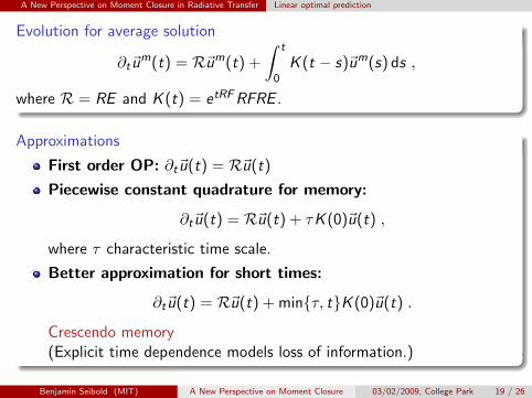
Evolution for average solution

∂t~um(t) = R~um(t) +

∫ t

0K (t − s)~um(s) ds ,

where R = RE and K (t) = etRF RFRE .

Approximations

First order OP: ∂t~u(t) = R~u(t)

Piecewise constant quadrature for memory:

∂t~u(t) = R~u(t) + τK (0)~u(t) ,

where τ characteristic time scale.

Better approximation for short times:

∂t~u(t) = R~u(t) + minτ, tK (0)~u(t) .

Crescendo memory(Explicit time dependence models loss of information.)



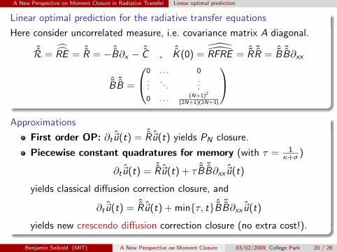
Linear optimal prediction for the radiative transfer equations

Here consider uncorrelated measure, i.e. covariance matrix A diagonal.

ˆR =RE = ˆR = − ˆB∂x − ˆC , ˆK (0) =

RFRE = ˆR ˜R = ˆB ˜B∂xx

ˆB ˜B =

0 . . . 0...

. . ....

0 . . .(N+1)2

(2N+1)(2N+3)

Approximations

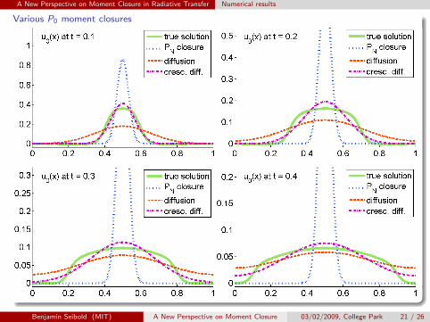
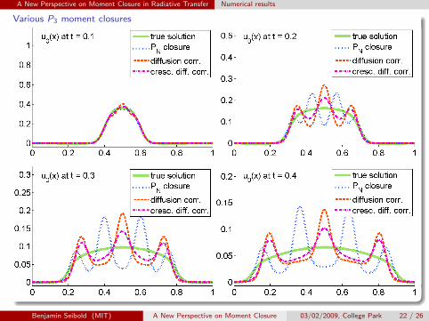
First order OP: ∂t~u(t) = ˆR~u(t) yields PN closure.

Piecewise constant quadratures for memory (with τ = 1κ+σ )

∂t~u(t) = ˆR~u(t) + τ ˆB ˜B∂xx~u(t)

yields classical diffusion correction closure, and

∂t~u(t) = ˆR~u(t) + minτ, t ˆB ˜B∂xx~u(t)

yields new crescendo diffusion correction closure (no extra cost!).


A New Perspective on Moment Closure in Radiative Transfer Numerical results

Various P0 moment closures



Various P3 moment closures



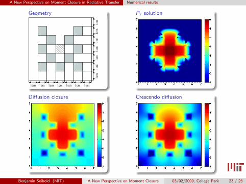
Geometry

1cm 1cm1cm1cm1cm1cm 1cm

1cm

1cm

1cm

1cm

1cm

1cm

1cm

P7 solution

Diffusion closure Crescendo diffusion


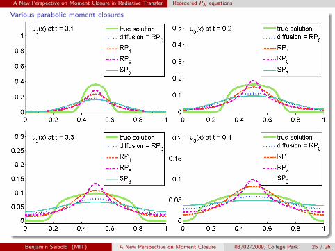
A New Perspective on Moment Closure in Radiative Transfer Reordered PN equations

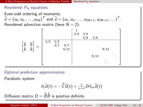
Reordered PN equations

Even-odd ordering of moments:~u = (u0, u2, . . . , u2N)T and ~u = (u1, u3, . . . , u2N+1, u2N+2, . . . )

T .Reordered advection matrix (here N = 2):

[ˆB ˆB˜B ˜B

]=

12/5 3/5

4/9 5/91/3 2/3

3/7 4/75/11 6/11

6/13. . .

. . .

Optimal prediction approximation

Parabolic system

∂t~u(t) = − ˆC~u(t) + 1κ+σD∂xx~u(t)

Diffusion matrix D = ˆB ˜B is positive definite.



Various parabolic moment closures



Conclusions

Optimal Prediction yields a new perspective on moment closure.

A wide variety of new closures can be derived by differentapproximations of the memory convolution.

Crescendo diffusion is a very simple modification to diffusion, thatincreases accuracy.

Future research directions

Solution and storage of the orthogonal dynamics.

Nonlinear measures ⇒ nonlinear closures?

More complex applications, application to kinetic gas dynamics.

M. Frank, B. S., Optimal prediction for radiative transfer: A new perspective on moment closure, arXiv:0806.4707 [math-ph]B. S., M. Frank, Optimal prediction for moment models: Crescendo diffusion and reordered equations, arXiv:0902.0076

http://www-math.mit.edu/~seibold/research/truncation

Thank you.


Documents

Optimal Prediction for Radiative Transfer: A New … Prediction for Radiative Transfer: A New Perspective on Moment Closure Benjamin Seibold MIT Applied Mathematics Mar 02nd, 2009