Embed Size (px)
Citation preview
Optimal Policy for Macro-Financial Stability∗
Gianluca BenignoLondon School of Economics
Huigang ChenJD Power
Christopher Otrok
University of Virginia
Alessandro Rebucci
Inter-American Development Bank
Eric R. YoungUniversity of Virginia
First Draft: November 2007;This Draft: April 28, 2011.
∗Earlier versions of this paper circulated under the titles ”Optimal Policy with Occasionally BindingCredit Constraints” and ”Optimal Stabilization Policy in a Model with Endogenous Sudden Stops”. Weare grateful to Javier Bianchi, Emine Boz, John Driffil, Robert Kollmann, Anton Korinek, Enrique Men-doza, Martin Uribe, and Michael Wickens for helpful comments and suggestions. We also thank seminarparticipants at the Bank of Brazil, Bank of Italy, BIS, Boston College, Cardiff University, CERGE-EI,Columbia University, the ECB, Federal Reserve Bank of Dallas, Federal Reserve Board, the Hong KongMonetary Authority, IGIER-Bocconi University, the IMF, Princeton University, UC-Berkeley, Universityof Iowa, University of Wisconsin, and participants at the Conference on Methods in Macroeconomics atUT-Dallas, Macroeconomics of Emerging Markets Conference at Colegio de Mexico, ESSIM 2009, NBERIFM Summer Institute 2009, and the Testing Open Economy Models Conference at the Bank of Greece forhelpful comments. Otrok thanks the Bankard Fund for Political Economy for Financial Support. Youngthanks the hospitality of the Richmond Fed. The views expressed in this paper are exclusively those of theauthors and not those of the Inter-American Development Bank or JD Power.
1
Abstract We study optimal policy in an small open economy in which a foreign bor-rowing constraint binds only occasionally and a financial crisis is an endogenous event. Inthis environment, the scope for policy arises because of a pecuniary externality stemmingfrom the presence of a key relative price in the borrowing constraint. We study how op-timal policy should be set. We first examine the merit of alternative policy tools. In theendowment case, we compare exchange rate policy and controls on capital flows and findthat exchange rate policy dominates capital controls since it replicates the unconstrainedfirst best allocation while capital controls achieve only the constrained efficient one. Inthis special endowment case, optimal policy (in the Ramsey sense) is time consistent andreplicates the social planner allocation. We then examine the case of a production econ-omy and compute the time-consistent optimal policy for alternative instruments confirmingthat, even in this more realistic case, exchange rate policy dominates capital controls butwith the important difference that, when used individually, neither of these policies canreplicate the constrained efficient outcome. For this reason, we examine the optimal useof the two policy instrument. A methodological contribution of the paper is the develop-ment of computational algorithms to solve optimal policy problems in environments withconstraints that bind only occasionally.
JEL Classification: E52, F37, F41Keywords: Capital Controls, Capital Flows, Exchange Rate Policy, Financial Frictions,
Financial Crises, Macro-Finacial Stability, Prudential Policies.
2
1 Introduction
The global financial crisis and ensuing great recession of 2007-2009 have ignited a debate on
the role of policy for the stability of the finacial system and hence the economy as a whole
(i.e., macro-financial stability). In advanced economies, this debate is revolving around the
role of monetary and regulatory policies in causing the global crisis and how the conduct of
monetary policy and supervision of financial intermediaries should be altered in the future.
In emerging markets, financial imperfections have long been recognized as an important
source of business cycle fluctuations and crises informing the debate on the relative merit
of alternative macroeconomic policy regimes. But the resurgence of very strong inflows of
foreign capital from advanced economies after the global crisis has refocused the ongoing
discussion on policies that are desirable from a macro-financial stability perspective.
The key question in this broad debate in advanced and emerging economies alike is
whether or how policy should act before a financial crisis strikes.1 In this paper we address
this general question in a Ramsey optimal policy framework and find that it is desirable
to intervene in a precautionary manner before a crisis strikes; how to intervene, however,
depends on the characteristics of the economy and the instruments that the policy maker
has available.
We address the general question above from the perspective of the economy as a whole
(i.e., the financial stability of the whole economy as opposed to specific sectors, or indi-
vidual intermediaries). A growing, related literature addresses the same issue with specific
reference to the financial sector or the regulation of individual financial intermediaries with
a system-wide stability objective in mind. That is we ask how much of a precautionary
component should there be in the optimal stabilization policy of the economy as a whole
in normal times? At what point before a possible financial crisis should the government
intervene with its instruments (e.g., monetary, fiscal, quasi fiscal, regulatory, etc.)? Should
the government wait until the crisis strikes, or should it intervene as the probability of the
crisis rises? In addressing these questions, we solve for optimal policy both in and away
from the crisis period.
These questions are meaningful only in a model in which there are both crisis and non-
crisis states and in which a crisis event is an endogenous outcome. We model financial crises
as a situation in which a financial friction (e.g., an international borrowing constraint in
our model) becomes binding. The constraint in our model binds endogenously, depending
1This is different than asking what is the optimal policy responses in models in which the economyis in a financial crisis (or a sudden stop of financial flows). On the latter, see for instance Braggion,Christiano, Roldos (2007), Caballero and Panageas (2007), Christiano, Gust, and Roldos (2004), Curdia(2007), Caballero and Krishnamurthy (2005), or Hevia (2008).
3
on agents’ choices as well as the state of the economy. When the constraint does not
bind the model economy exhibits normal business cycle fluctuations. The presence of the
borrowing constraint, though, leaves the economy vulnerable to the possibility that a small
negative shock pushes it into the binding region, for certain levels of indebtedness. When
this happens, the economy enters a crisis state and suffers the economic dislocation typically
associated with a financial crisis episode.
Our endogenous borrowing credit constraint is embedded in a standard two-sector (trad-
able and non-tradable good) small open economy (e.g., Obstfeld and Rogoff, 1996, Chapter
4) in which financial markets are not only incomplete but also imperfect, as in Mendoza
(2002, 2010). The asset menu is restricted to a one period risk-free bond paying off the ex-
ogenously given foreign interest rate. In addition, we assume that access to foreign financing
is constrained to a fraction of households’ total income. Foreign borrowing is denominated
in units of the tradable good but it is leveraged on income generated at different rela-
tive prices (i.e. the relative price of non-tradeable good), a specification of the borrowing
constraint that captures “liability dollarization” a key feature of emerging market capital
structure (e.g., Krugman 2002).2
Within this framework, a scope for policy arises because of a price externality (or a
pecuniary or credit externality) stemming from the presence of a key market price in the
occasionally binding financial friction (see also Benigno et al. (2010, 2011), Bianchi (2011),
Binachi and Mendoza (2010), Caballero and Lorenzoni (2008), Chang, Cespedes, and Ve-
lasco (2011), Jeanne and Korinek (2010), Korinek (2008), or Lorenzoni (2008)) who analyze
the same kind of externality). Individual agents take prices as given and do not internalize
the effect of their individual decisions on a key market price that enters the specification of
the financial friction—see Arnott, Greenwald, and Stiglitz (1994) for a discussion. Because
of this externality, it has been shown that in models like the one we analyze the competitive
equilibrium is constrained inefficient. This inefficiency is typically measured and quantified
by comparing the competitive equilibrium (CE) of the economy with the amount that a
social planner would choose in an economy subject to the same occasionally binding credit
constraint (SP).
The policy analysis is than conducted by choosing a policy instrument and determin-
ing the policy rule that implements the constrained efficient allocation under commitment
(e.g., Bianchi 2011). The social planner approach provides a useful normative benchmark
but is not necessarily useful to design actual policies to move the economy toward it. One
important limitation of this approach is that the social planner is assumed to be able to
commit in advance to a full set of state contingent policies. In this set up, however, there
2The latest wave of crises in emerging Europe is striking evidence of the importance of such feature.
4
is no interaction between the policy maker and the private sector, thus omitting to con-
sider time-consistency considerations, a fundamental aspect of the typical macroeconomic
stabilization problems—e.g., Kydland and Prescott (1977). In contrasts with the existing
literature, an important contribution of our paper is to allow for this interaction in the
analysis of the key policy question in the ongoing policy debate. Specifically, in this pa-
per we develop optimal policies to address the same pecuniary externality analyzed in the
literature under discretion. These policies are the optimal responses of a government that
is unable to commit to policies in advance and must decide period by period how to set
policy. Our optimal policy approach is more closely related to the problem faced by actual
governments that are unable to commit in advance to a set of policies. 3
To our knowledge, there are no contributions in the literature on the analysis of opti-
mal policy in an environment in which a borrowing constraint both binds occasionally and
is endogenous to the decisions in the model. The most closely related work to ours are
Adams and Billi (2006a,2006b), who study optimal monetary policy in a closed economy,
new Keynesian model in which there is zero lower bound on interest rates. Their zero-
bound constraint is fixed and does not evolve endogenously. Bordo and Jeanne (2002) and
Devereaux and Poon (2004), Jeanne and Korinek (2011) investigate precautionary compo-
nents of optimal monetary policy responses to asset prices and sudden stops, respectively,
but not in the context of fully-specified DSGE models. We thus address key economic
and computational issues related to the design of optimal policy with occasionally binding
financial frictions.
To solve for optimal policy in this model we develop a global solution method. That is,
we solve for a policy rule across both states of the world, when the constraint binds and when
it does not. Such an approach enforces that the rule away from the crisis periods is designed
with full knowledge of what the rule will be when the economy enters the sudden stop. This
statement holds for both the policymaker and the agents in the economy. This solution
method, while computationally costly, is critical for understanding the interaction between
precautionary behavior on the part of the private sector with precautionary behavior on
the part of the policy maker. The technical challenge in solving such a model is that the
constraint binds only occasionally and changes location in the state space of the model
depending on the state of the economy.
We employ two tax instruments in our optimal policy exercise. The first is a distor-
tionary tax on non-traded consumption, which can be interpreted as exchange rate policy.
3As Chari and Kehoe (2010) note, discretion is a more realistic assumption. While a social plannerwill be able to reach an equilibrium with higher welfare than the optimal policy, gains from the optimalpolicies we solve for are more in line with the actual constraints faced by governments, particularly thosein emerging markets.
5
The second is a tax on debt and can be interpreted as a control on capital flows (or a cap-
ital control for brevity). In both cases, tax policy is financed through lump-sum transfers
so that the government budget constraint is balanced in each period. Ideally one would
like to analyze optimal policy for macro-financial stability alongside a more traditional sta-
bilization objective (i.e., monetary, fiscal, external). However, computational limitations
restrict the analysis to the sole macro-financial stability objective (see below on this). This
means that, if we were to remove the friction that is the source of financial instability in
the economy, optimal policy would be ”no action” in all periods and states of the world.
The main results of the analysis are as follows. In an endowment version of our economy
(i.e., Bianchi, 2011), if the policy maker has only one instrument, we find analytically that
(i) a tax or subsidy on consumption (i.e., exchange rate policy) can achieve the first best
allocation, while a tax or subsidy on foreign borrowing (i.e., a capital control) can only
achieve a second best allocation; (ii) Ramsey optimal policy under discretion is the same as
under commitment and achieves the same allocation selected by a social planner that is not
constrained by the behavior of the private sector. In a production version of our economy
(i.e., Benigno et al. 2011), we find numerically that, (iii) if the Ramsey planner has only
one instrument with discretion, the optimal intervention is a prudential tax regardless of
the instrument used. However (iv), if the Ramsey planner has both a consumption tax and
a tax on debt as instruments (e.g., Jeanne and Korinek, 2011), the optimal intervention is
a tax on debt and a subsidy on consumption during financial crises and no intervention in
normal times. Finally, we also find numerically that (v) exchange rate policy dominates
capital controls if the Ramsey planner has only one instrument with discretion, and neither
achieves the second best constrained efficient allocation selected by a social planner in our
production economy. The results reported have a number of general policy implications for
macro-financial stability.
The rest of the paper is organized as follows. Section 2 presents analytic results from an
endowment economy. Section 3 describes the fully specified DSGE model we use. Section
4 discusses the notion of equilibria that we compute and describe the solution methods.
Section 5 calibrates the model and evaluate its performance against the data. Section 5
reports the numerical analysis of the production economy we consider, characterizing the
optimal policy and discussing its working. Section 7 concludes.
6
2 Optimal Policies in a Two-Goods Endowment Econ-
omy
Before turning to our general model, we first discuss the optimal policy problem for its
simpler version, an endowment economy, which can be solved analytically with one alter-
native policy instrument at the time. There are two reasons to do so. First, we want to
understand the relationship between the social planner problem and optimal policies with
and without commitment. Second, we use this analysis to gain some intuition for the work-
ing of the instruments we choose in the more general optimal policy problem that we solve
numerically.
2.1 Tax on Non-Tradable Consumption (Exchange Rate Policy)
Consider the two-goods endowment economy studied by Korinek (2009) and Bianchi (2010).
In the first case, we study the taxation on non-tradable consumption (this policy tool can
be interpreted in terms of managing the exchange rate).
2.1.1 Competitive Equilibrium
The competitive equilibrium of this economy is characterized as follows. There is a contin-
uum of households j ∈ [0, 1] that maximize the utility function
U j ≡ E0
∞∑t=0
{βt 1
1− ρ(Cj,t)
1−ρ
}, (1)
with Cj denoting the individual consumption basket. The consumption basket, Ct, is a
composite of tradable and non-tradable goods:
Ct ≡[ω
1κ
(CT
t
)κ−1κ + (1− ω)
1κ(CN
t
)κ−1κ
] κκ−1
. (2)
The parameter κ is the elasticity of intratemporal substitution between consumption of
tradable and nontradable goods, while ω is the relative weight of the two goods in the
utility function.
We normalize the price of traded goods to 1. The relative price of the nontraded good
is denoted PN . The aggregate price index is then given by
Pt =[ω + (1− ω)
(PNt
)1−κ] 1
1−κ
,
7
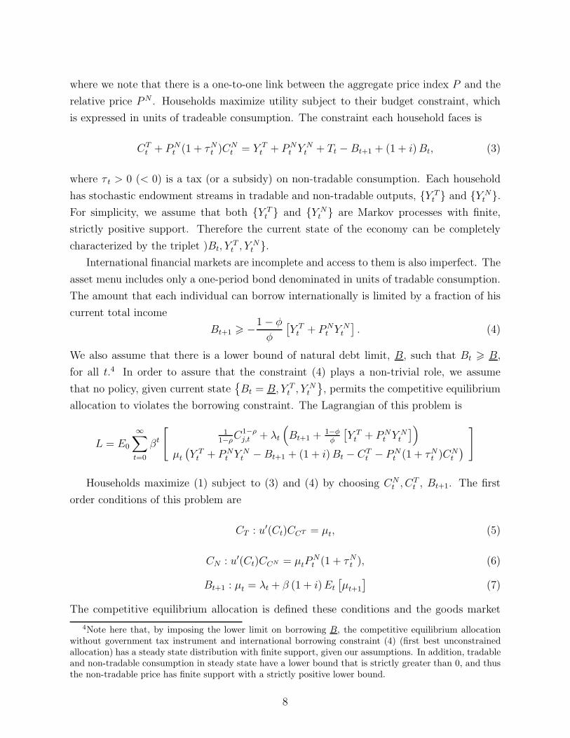
where we note that there is a one-to-one link between the aggregate price index P and the
relative price PN . Households maximize utility subject to their budget constraint, which
is expressed in units of tradeable consumption. The constraint each household faces is
CTt + PN
t (1 + τNt )CNt = Y T
t + PNt Y N
t + Tt − Bt+1 + (1 + i)Bt, (3)
where τ t > 0 (< 0) is a tax (or a subsidy) on non-tradable consumption. Each household
has stochastic endowment streams in tradable and non-tradable outputs, {Y Tt } and {Y N
t }.For simplicity, we assume that both {Y T
t } and {Y Nt } are Markov processes with finite,
strictly positive support. Therefore the current state of the economy can be completely
characterized by the triplet )Bt, YTt , Y N
t }.International financial markets are incomplete and access to them is also imperfect. The
asset menu includes only a one-period bond denominated in units of tradable consumption.
The amount that each individual can borrow internationally is limited by a fraction of his
current total income
Bt+1 � −1 − φ
φ
[Y Tt + PN
t Y Nt
]. (4)
We also assume that there is a lower bound of natural debt limit, B, such that Bt � B,
for all t.4 In order to assure that the constraint (4) plays a non-trivial role, we assume
that no policy, given current state{Bt = B, Y T
t , Y Nt
}, permits the competitive equilibrium
allocation to violates the borrowing constraint. The Lagrangian of this problem is
L = E0
∞∑t=0
βt
[1
1−ρC1−ρ
j,t + λt
(Bt+1 +
1−φφ
[Y Tt + PN
t Y Nt
])μt
(Y Tt + PN
t Y Nt −Bt+1 + (1 + i)Bt − CT
t − PNt (1 + τNt )C
Nt
)]
Households maximize (1) subject to (3) and (4) by choosing CNt , CT
t , Bt+1. The first
order conditions of this problem are
CT : u′(Ct)CCT = μt, (5)
CN : u′(Ct)CCN = μtPNt (1 + τN
t ), (6)
Bt+1 : μt = λt + β (1 + i)Et
[μt+1
](7)
The competitive equilibrium allocation is defined these conditions and the goods market
4Note here that, by imposing the lower limit on borrowing B, the competitive equilibrium allocationwithout government tax instrument and international borrowing constraint (4) (first best unconstrainedallocation) has a steady state distribution with finite support, given our assumptions. In addition, tradableand non-tradable consumption in steady state have a lower bound that is strictly greater than 0, and thusthe non-tradable price has finite support with a strictly positive lower bound.
8
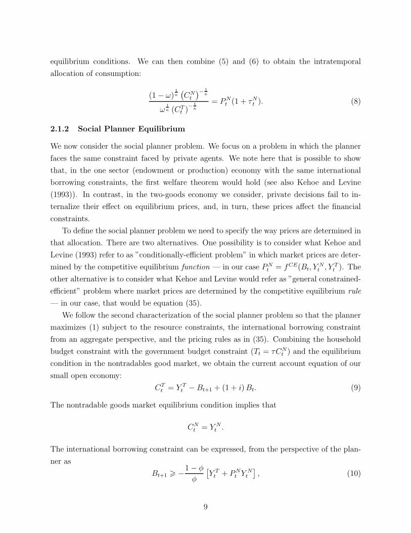
equilibrium conditions. We can then combine (5) and (6) to obtain the intratemporal
allocation of consumption:
(1− ω)1κ(CN
t
)− 1κ
ω1κ (CT
t )− 1
κ
= PNt (1 + τNt ). (8)
2.1.2 Social Planner Equilibrium
We now consider the social planner problem. We focus on a problem in which the planner
faces the same constraint faced by private agents. We note here that is possible to show
that, in the one sector (endowment or production) economy with the same international
borrowing constraints, the first welfare theorem would hold (see also Kehoe and Levine
(1993)). In contrast, in the two-goods economy we consider, private decisions fail to in-
ternalize their effect on equilibrium prices, and, in turn, these prices affect the financial
constraints.
To define the social planner problem we need to specify the way prices are determined in
that allocation. There are two alternatives. One possibility is to consider what Kehoe and
Levine (1993) refer to as ”conditionally-efficient problem” in which market prices are deter-
mined by the competitive equilibrium function — in our case PNt = fCE(Bt, Y
Nt , Y T
t ). The
other alternative is to consider what Kehoe and Levine would refer as ”general constrained-
efficient” problem where market prices are determined by the competitive equilibrium rule
— in our case, that would be equation (35).
We follow the second characterization of the social planner problem so that the planner
maximizes (1) subject to the resource constraints, the international borrowing constraint
from an aggregate perspective, and the pricing rules as in (35). Combining the household
budget constraint with the government budget constraint (Tt = τCNt ) and the equilibrium
condition in the nontradables good market, we obtain the current account equation of our
small open economy:
CTt = Y T
t −Bt+1 + (1 + i)Bt. (9)
The nontradable goods market equilibrium condition implies that
CNt = Y N
t .
The international borrowing constraint can be expressed, from the perspective of the plan-
ner as
Bt+1 � −1 − φ
φ
[Y Tt + PN
t Y Nt
], (10)
9

where the relative price is determined by the competitive rule (35). This condition allows
us to rewrite (4) as
Bt+1 � −1− φ
φ
⎡⎣Y T
t +
((1− ω)
(CT
t
)ωY N
t
) 1κ
(1 + τNt )Y
Nt
⎤⎦ .
The Lagrangian of the planner problem becomes
L = E0
∞∑t=0
βt
⎡⎢⎣
11−ρ
(Cj,t)1−ρ + μ1,t
(Y Tt − Bt+1 + (1 + i)Bt − CT
t
)+
+μ2,t
(Y Nt − CN
t
)+ λt
(Bt+1 +
1−φφ
[Y Tt +
((1−ω)(CT
t )ωY N
t
) 1κ
(1 + τNt )YN
]) ⎤⎥⎦ ,
in which the planner chooses the optimal path of CTt , C
Nt , Bt+1. The first order conditions
for the planner problem are given by
CT : u′(Ct)CCT = μ1,t − λtΣt, (11)
CN : u′(Ct)CCN = μ2,t, (12)
Bt+1 : μ1,t = λt + β (1 + i)Et
[μ1,t+1
]. (13)
where
Σt ≡ 1− φ
φ
∂PNt
∂CTt
Y Nt =
1− φ
φ
1
κ
(1− ω)
ω
((1− ω)
(CT
t
)ω
) 1κ−1
(1 + τNt )(Y Nt
)κ−1κ .
Note here that Σt contains the instrument (1 + τNt ).
We now discuss the extent to which it is possible to use (1+τNt ) in the competitive equi-
librium allocation to replicate the social planner equilibrium. The planner Euler equation
can be rewritten as
u′(Ct)CCT + λtΣt =
λt + β (1 + i)Et [u′(Ct+1)CCT + λΣt+1]
with
λt
⎡⎣Bt+1 +
1− φ
φ
⎡⎣Y T +
((1− ω)
(CT
t
)ωY N
) 1κ
(1 + τNt )YN
⎤⎦⎤⎦ = 0.
10
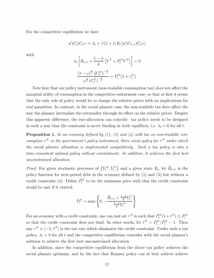
For the competitive equilibrium we have
u′(Ct)CCT = λt + β (1 + i)Et [u′(Ct+1)CCT ]
with
λt
[Bt+1 +
1− φ
φ
[Y T + PN
t Y N]]
= 0
(1− ω)1κ(CN
t
)− 1κ
ω1κ (CT
t )− 1
κ
= PNt (1 + τNt ).
Note here that our policy instrument (non-tradable consumption tax) does not affect the
marginal utility of consumption in the competitive endowment case, so that at first it seems
that the only role of policy would be to change the relative prices with no implications for
real quantities. In contrast, in the social planner case, the non-tradable tax does affect the
way the planner internalize the externality through its effect on the relative prices. Despite
this apparent difference, the two-allocation can coincide: tax policy needs to be designed
in such a way that the constraint is never binding in both equilibria, i.e. λt = 0 for all t.
Proposition 1. In an economy defined by (1), (3) and (4) with tax on non-tradable con-
sumption τN as the government’s policy instrument, there exists policy for τN under which
the social planner allocation is implemented competitively. Such a tax policy is also a
time-consistent optimal policy without commitment. In addition, it achieves the first best
unconstrained allocation.
Proof. For given stochastic processes of{Y Nt , Y T
t
}and a given state Bt, let Bt+1 is the
policy function for next-period debt in the economy defined by (1) and (3) but without a
credit constraint (4). Define PNt to be the minimum price such that the credit constraint
would be met if it existed,
PNt = max
{0,−Bt+1 +
1−φφY Tt
1−φφY Nt
}.
For an economy with a credit constraint, one can just set τN is such that PNt (1+τN ) ≤ PN
t
so that the credit constraint does not bind. In other words, let τN = PNt /PN
t − 1. Then
any τN ∈ (−1, τN ] is the tax rate which eliminates the credit constraint. Under such a tax
policy, λt = 0 for all t and the competitive equilibrium coincides with the social planner’s
solution to achieve the first best unconstrained allocation.
In addition, since the competitive equilibrium from the above tax policy achieves the
social planner optimum, and by the fact that Ramsey policy can at best achieve achieve
11
the social planner optimum, we reach the conclusion that the tax policy is also a Ramsey
solution. Such policy is completely determined by the current state {Bt, YTt , Y N
t } and
therefore it is time-consistent.
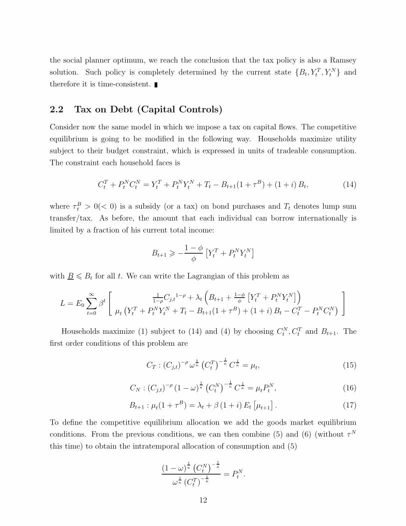
2.2 Tax on Debt (Capital Controls)
Consider now the same model in which we impose a tax on capital flows. The competitive
equilibrium is going to be modified in the following way. Households maximize utility
subject to their budget constraint, which is expressed in units of tradeable consumption.
The constraint each household faces is
CTt + PN
t CNt = Y T
t + PNt Y N
t + Tt − Bt+1(1 + τB) + (1 + i)Bt, (14)
where τBt > 0(< 0) is a subsidy (or a tax) on bond purchases and Tt denotes lump sum
transfer/tax. As before, the amount that each individual can borrow internationally is
limited by a fraction of his current total income:
Bt+1 � −1 − φ
φ
[Y Tt + PN
t Y Nt
]with B � Bt for all t. We can write the Lagrangian of this problem as
L = E0
∞∑t=0
βt
[1
1−ρCj,t
1−ρ + λt
(Bt+1 +
1−φφ
[Y Tt + PN
t Y Nt
])μt
(Y Tt + PN
t Y Nt + Tt −Bt+1(1 + τB) + (1 + i)Bt − CT
t − PNt CN
t
)]
Households maximize (1) subject to (14) and (4) by choosing CNt , CT
t and Bt+1. The
first order conditions of this problem are
CT : (Cj,t)−ρ ω
1κ
(CT
t
)− 1κ C
1κ = μt, (15)
CN : (Cj,t)−ρ (1− ω)
1κ(CN
t
)− 1κ C
1κ = μtP
Nt , (16)
Bt+1 : μt(1 + τB) = λt + β (1 + i)Et
[μt+1
]. (17)
To define the competitive equilibrium allocation we add the goods market equilibrium
conditions. From the previous conditions, we can then combine (5) and (6) (without τN
this time) to obtain the intratemporal allocation of consumption and (5)
(1− ω)1κ(CN
t
)− 1κ
ω1κ (CT
t )− 1
κ
= PNt .
12
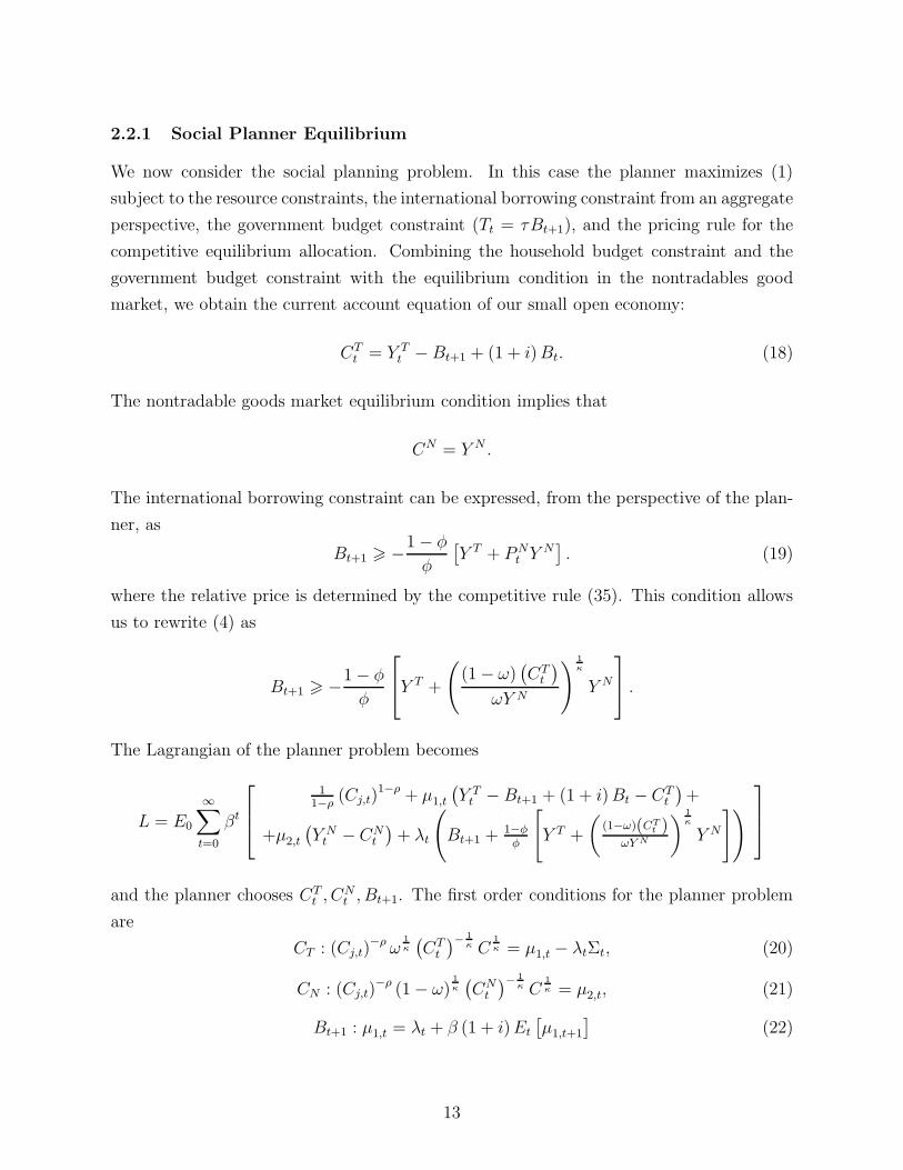
2.2.1 Social Planner Equilibrium
We now consider the social planning problem. In this case the planner maximizes (1)
subject to the resource constraints, the international borrowing constraint from an aggregate
perspective, the government budget constraint (Tt = τBt+1), and the pricing rule for the
competitive equilibrium allocation. Combining the household budget constraint and the
government budget constraint with the equilibrium condition in the nontradables good
market, we obtain the current account equation of our small open economy:
CTt = Y T
t −Bt+1 + (1 + i)Bt. (18)
The nontradable goods market equilibrium condition implies that
CN = Y N .
The international borrowing constraint can be expressed, from the perspective of the plan-
ner, as
Bt+1 � −1 − φ
φ
[Y T + PN
t Y N]. (19)
where the relative price is determined by the competitive rule (35). This condition allows
us to rewrite (4) as
Bt+1 � −1− φ
φ
⎡⎣Y T +
((1− ω)
(CT
t
)ωY N
) 1κ
Y N
⎤⎦ .
The Lagrangian of the planner problem becomes
L = E0
∞∑t=0
βt
⎡⎢⎣
11−ρ
(Cj,t)1−ρ + μ1,t
(Y Tt − Bt+1 + (1 + i)Bt − CT
t
)+
+μ2,t
(Y Nt − CN
t
)+ λt
(Bt+1 +
1−φφ
[Y T +
((1−ω)(CT
t )ωY N
) 1κ
Y N
]) ⎤⎥⎦
and the planner chooses CTt , C
Nt , Bt+1. The first order conditions for the planner problem
are
CT : (Cj,t)−ρ ω
1κ
(CT
t
)− 1κ C
1κ = μ1,t − λtΣt, (20)
CN : (Cj,t)−ρ (1− ω)
1κ(CN
t
)− 1κ C
1κ = μ2,t, (21)
Bt+1 : μ1,t = λt + β (1 + i)Et
[μ1,t+1
](22)
13
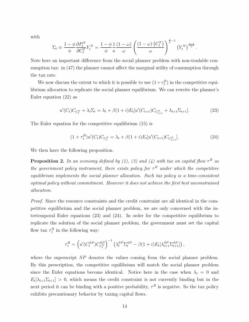
with
Σt ≡ 1− φ
φ
∂PNt
∂CTt
Y Nt =
1− φ
φ
1
κ
(1− ω)
ω
((1− ω)
(CT
t
)ω
) 1κ−1 (
Y Nt
)κ−1κ .
Note here an important difference from the social planner problem with non-tradable con-
sumption tax: in (47) the planner cannot affect the marginal utility of consumption through
the tax rate.
We now discuss the extent to which it is possible to use (1+τBt ) in the competitive equi-
librium allocation to replicate the social planner equilibrium. We can rewrite the planner’s
Euler equation (22) as
u′(Ct)CCTt+ λtΣt = λt + β(1 + i)Et[u
′(Ct+1)CCTt+1
+ λt+1Σt+1]. (23)
The Euler equation for the competitive equilibrium (15) is
(1 + τBt )u′(Ct)CCT
t= λt + β(1 + i)Et[u
′(Ct+1)CCTt+1
]. (24)
We then have the following proposition.
Proposition 2. In an economy defined by (1), (3) and (4) with tax on capital flow τB as
the government policy instrument, there exists policy for τB under which the competitive
equilibrium implements the social planner allocation. Such tax policy is a time-consistent
optimal policy without commitment. However it does not achieve the first best unconstrained
allocation.
Proof. Since the resource constraints and the credit constraint are all identical in the com-
petitive equilibrium and the social planner problem, we are only concerned with the in-
tertemporal Euler equations (23) and (24). In order for the competitive equilibrium to
replicate the solution of the social planner problem, the government must set the capital
flow tax τBt in the following way:
τBt =
(u′(CSP
t )CSPCT
t
)−1 (λSPt ΣSP
t − β(1 + i)Et[λSPt+1Σ
SPt+1]),
where the superscript SP denotes the values coming from the social planner problem.
By this prescription, the competitive equilibrium will match the social planner problem
since the Euler equations become identical. Notice here in the case when λt = 0 and
Et[λt+1Σt+1] > 0, which means the credit constraint is not currently binding but in the
next period it can be binding with a positive probability, τB is negative. So the tax policy
exhibits precautionary behavior by taxing capital flows.
14
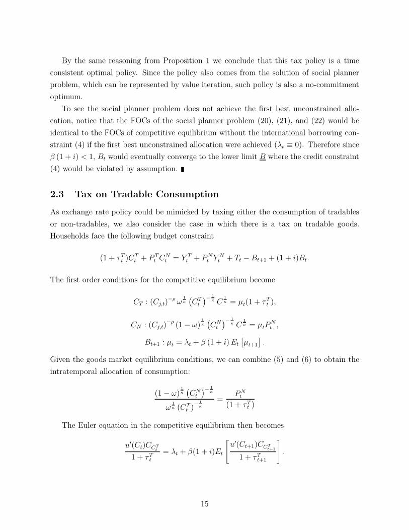
By the same reasoning from Proposition 1 we conclude that this tax policy is a time
consistent optimal policy. Since the policy also comes from the solution of social planner
problem, which can be represented by value iteration, such policy is also a no-commitment
optimum.
To see the social planner problem does not achieve the first best unconstrained allo-
cation, notice that the FOCs of the social planner problem (20), (21), and (22) would be
identical to the FOCs of competitive equilibrium without the international borrowing con-
straint (4) if the first best unconstrained allocation were achieved (λt ≡ 0). Therefore since
β (1 + i) < 1, Bt would eventually converge to the lower limit B where the credit constraint
(4) would be violated by assumption.
2.3 Tax on Tradable Consumption
As exchange rate policy could be mimicked by taxing either the consumption of tradables
or non-tradables, we also consider the case in which there is a tax on tradable goods.
Households face the following budget constraint
(1 + τTt )C
Tt + P T
t CNt = Y T
t + PNt Y N
t + Tt −Bt+1 + (1 + i)Bt.
The first order conditions for the competitive equilibrium become
CT : (Cj,t)−ρ ω
1κ
(CT
t
)− 1κ C
1κ = μt(1 + τT
t ),
CN : (Cj,t)−ρ (1− ω)
1κ(CN
t
)− 1κ C
1κ = μtP
Nt ,
Bt+1 : μt = λt + β (1 + i)Et
[μt+1
].
Given the goods market equilibrium conditions, we can combine (5) and (6) to obtain the
intratemporal allocation of consumption:
(1− ω)1κ(CN
t
)− 1κ
ω1κ (CT
t )− 1
κ
=PNt
(1 + τTt )
The Euler equation in the competitive equilibrium then becomes
u′(Ct)CCTt
1 + τTt= λt + β(1 + i)Et
[u′(Ct+1)CCT
t+1
1 + τTt+1
].
15
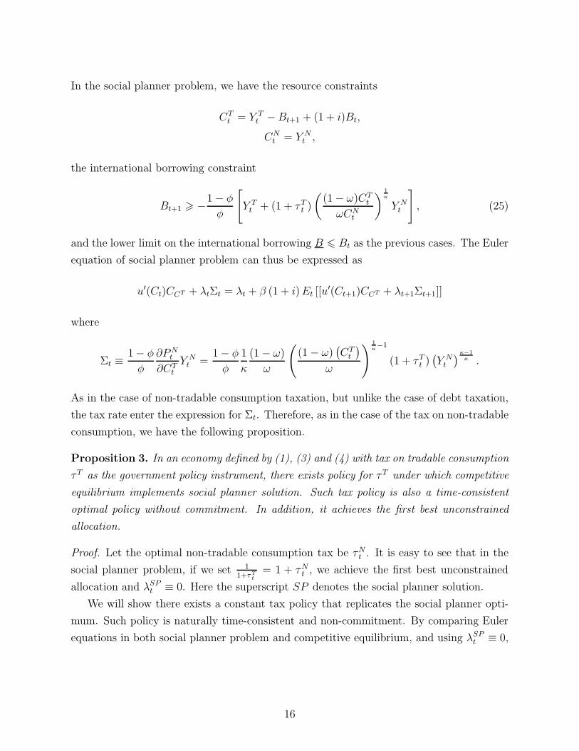
In the social planner problem, we have the resource constraints
CTt = Y T
t −Bt+1 + (1 + i)Bt,
CNt = Y N
t ,
the international borrowing constraint
Bt+1 � −1− φ
φ
[Y Tt + (1 + τT
t )
((1− ω)CT
t
ωCNt
) 1κ
Y Nt
], (25)
and the lower limit on the international borrowing B � Bt as the previous cases. The Euler
equation of social planner problem can thus be expressed as
u′(Ct)CCT + λtΣt = λt + β (1 + i)Et [[u′(Ct+1)CCT + λt+1Σt+1]]
where
Σt ≡ 1− φ
φ
∂PNt
∂CTt
Y Nt =
1− φ
φ
1
κ
(1− ω)
ω
((1− ω)
(CT
t
)ω
) 1κ−1
(1 + τTt )(Y Nt
)κ−1κ .
As in the case of non-tradable consumption taxation, but unlike the case of debt taxation,
the tax rate enter the expression for Σt. Therefore, as in the case of the tax on non-tradable
consumption, we have the following proposition.
Proposition 3. In an economy defined by (1), (3) and (4) with tax on tradable consumption
τT as the government policy instrument, there exists policy for τT under which competitive
equilibrium implements social planner solution. Such tax policy is also a time-consistent
optimal policy without commitment. In addition, it achieves the first best unconstrained
allocation.
Proof. Let the optimal non-tradable consumption tax be τNt . It is easy to see that in the
social planner problem, if we set 11+τT
t= 1 + τN
t , we achieve the first best unconstrained
allocation and λSPt ≡ 0. Here the superscript SP denotes the social planner solution.
We will show there exists a constant tax policy that replicates the social planner opti-
mum. Such policy is naturally time-consistent and non-commitment. By comparing Euler
equations in both social planner problem and competitive equilibrium, and using λSPt ≡ 0,
16
it is sufficient to find τTt so that
1
1 + τTt
=
Et
[u′(CSP
t+1)CSP
CTt+1
1+τTt+1
]
Et[u′(CSPt+1)C
SPCT
t+1], (26)
and the international borrowing constraint (25) is satisfied, in order for the competitive
equilibrium to achieve social planner optimum.
First we note that a constant tax policy will satisfy (26). Secondly, by our observation of
the first best unconstrained allocation, non-tradable price has strictly positive lower limit.
Therefore there exists τT such that the borrowing constraint (25) is always satisfied for any
τT � τT ). So any constant tax policy of the form τTt ≡ τT � τT ) is an optimal policy such
that the competitive equilibrium replicates the social planner optimal.
Whether exchange rate policy is enacted by taxing the tradable or the non-tradable
sector does not affect the main results of this part of the analysis. In the rest of the paper
we shall focus only on tax on debt and tax on non-tradable consumption.
3 A Two-Good, Two-Sector Production Economy
In this section we present the two-good, two-sector production economy in which we will
study optimal policy numerically. This is the same simple two-good (tradable and non-
tradable) small open economy discussed above, in which financial markets are not only
incomplete but also imperfect like in Mendoza (2010), and in which production occurs in
both sectors as in the model used by Benigno et al. (2011).
3.1 Households
There is a continuum of households j ∈ [0, 1] that maximize the utility function
U j ≡ E0
∞∑t=0
⎧⎨⎩βt 1
1− ρ
(Cj,t −
Hδj,t
δ
)1−ρ⎫⎬⎭ , (27)
with Cj denoting the individual consumption basket and Hj the individual supply of labor
for the tradeable and non-tradeable sectors (Hj = HTj +HN
j ). The assumption of perfect
substitutability between labor services in the two sectors insures that there is a unique
labor market. For simplicity we omit the j subscript for the remainder of this section,
17
but it is understood that all choices are made at the individual level. The elasticity of
labor supply is δ, while ρ is the coefficient of relative risk aversion. In (27), the preference
specification follows from Greenwood, Hercowitz and Huffman (1988) (hereafter, GHH).
In the context of a one-good economy this specification eliminates the wealth effect from
the labor supply choice. Here it is important to emphasize that in a multi-good economy,
the sectoral allocation of consumption will affect the labor supply decision through relative
prices.
As before, the consumption basket, Ct, is a composite of tradable and non-tradable
goods:
Ct ≡[ω
1κ
(CT
t
)κ−1κ + (1− ω)
1κ(CN
t
)κ−1κ
] κκ−1
. (28)
The parameter κ is the elasticity of intratemporal substitution between consumption of
tradable and nontradable goods, while ω is the relative weight of tradable goods in the
consumption basket. We normalize the price of traded goods to 1. The relative price of the
nontradable good is denoted PN . The aggregate price index is then given by
Pt =[ω + (1− ω)
(PNt
)1−κ] 1
1−κ,
where we note that there is a one to one link between the aggregate price index P and the
relative price PN .
Households maximize utility subject to their budget constraint, which is expressed in
units of tradeable consumption. The constraint each household faces is:5
CTt + PN
t CNt = πt +WtHt − Bt+1 + (1 + i)Bt, (29)
where Wt is the wage in units of tradable goods, Bt+1 denotes the net foreign asset position
at the end of period t with gross real return 1 + i. Households receive profits, πt, from
owning the representative firm. Their labor income is given by WtHt.
International financial markets are incomplete and access to them is also imperfect. The
asset menu includes only a one-period bond denominated in units of tradable consumption.
In addition, we assume that the amount that each individual can borrow internationally is
limited by a fraction of his current total income:
Bt+1 ≥ −1− φ
φ[πt +WtHt] . (30)
5Note here that, as we want to compute optimal policy for alternative instruments, and also theircombined use, the government is not explicitly introduced in the agent’s budget constraint to keep thenotation manageable.
18
This constraint captures a balance sheet effect (e.g., Krugman (1999) and Aghion, Bacchetta
and Banerjee (2004)) since foreign borrowing is denominated in units of tradables while the
income that can be pledged as collateral is generated also in the non-tradable sector. The
value of the collateral is endogenous in this model as it depends on the current realization
of profits and wage income. We don’t derive explicitly the credit constraint as the outcome
of an optimal contract between lenders and borrowers. However, we can interpret this
constraint as the outcome of an interaction between lenders and borrowers in which the
lenders is not willing to permit borrowing beyond a certain limit.6 This limit depends on
the parameter φ that measures the tightness of the borrowing constraint and it depends on
current income that could be used as a proxy of future income.7
Households maximize (27) subject to (29) and (30) by choosing CNt , CT
t , Bt+1, and Ht.
The first order conditions of this problem are
CT :
(Cj,t −
Hδj,t
δ
)−ρ
ω1κ
(CT
t
)− 1κ C
1κ = μt, (31)
CN :
(Cj,t −
Hδj,t
δ
)−ρ
(1− ω)1κ(CN
t
)− 1κ C
1κ = μtP
Nt , (32)
Bt+1 : μt = λt + β (1 + i)Et
[μt+1
], (33)
and
Ht :
(Cj,t −
Hδj,t
δ
)−ρ (Hδ−1
j,t
)= μtWt +
1− φ
φWtλt. (34)
μt is the multiplier on the period budget constraint and λt is the multiplier on the inter-
national borrowing constraint. When the credit constraint is binding (λt > 0), the Euler
equation (33) incorporates an effect that can be interpreted as arising from a country-
specific risk premium on external financing. In this framework, even if the constraint is
not binding at time t, there is an intertemporal effect coming from the possibility that the
constraint might be binding in the future. This effect is embedded in the term Et
[μt+1
],
6As emphasized by Arellano and Mendoza (2003), this form of liquidity constraint shares some features,namely the endogeneity of the risk premium, that would be the outcome of the interaction between a risk-averse borrower and a risk-neutral lender in a contracting framework as in Eaton and Gersovitz (1981). Itis also consistent with anecdotal evidence on lending criteria and guidelines used in mortgage and consumerfinancing.
7As we discuss in Benigno et al. (2009), a constraint expressed in terms of future income which could bethe outcome of the interaction between lenders and borrowers in a limited commitment environment wouldintroduce further computational difficulties that we need to avoid for tractability. If future consumptionchoices affect current borrowing decisions the planning problem would not be time-consistent in the usualset of state variables.
19
which implies that current consumption of tradeable goods would be lower compared to an
economy in which access to foreign borrowing is unconstrained.
From the previous conditions, we can combine (31) and (32) to obtain the intratem-
poral allocation of consumption and (31) with (34) to obtain the labor supply schedule,
respectively:
PNt =
(1− ω)1κ(CN
t
)− 1κ
ω1κ (CT
t )− 1
κ
(35)
(Hδ−1
j,t
)=
(ωC
CT
) 1κ
Wt
(1 +
1− φ
φ
λt
μt
). (36)
Note here that (ωC
CT
) 1κ
= (ω)1
κ−1
(1 +
(1− ω
ω
)(PNt
)1−κ) 1
κ−1
.
If we were in a one good economy model, there would be no effect coming from the marginal
utility of consumption on the labor supply choice because of the GHH preference specifi-
cation. In a two-sector model, however, a decrease in PN increases(ωCCT
) 1κ , and the labor
supply curve becomes steeper as PN falls.8 Note also that, when the constraint is binding
(λt > 0), the marginal utility of supplying one more unit of labor is higher, and this helps to
relax the constraint: when λt > 0, the labor supply becomes steeper and agents substitute
leisure with labor to increase the value of their collateral for given wages and prices. Given
that PN falls when the constraint is binding, these two effects imply an increase in labor
supply for given wages in the constrained region.
Importantly, the labor supply is also affected by the possibility that the constraint may
be binding in the future. If in period t the constraint is not binding but it may bind in
period t+ 1, we have (Cj,t −
Hδj,t
δ
)−ρ (Hδ−1
j,t
)= μtWt
and
μt = β (1 + i)Et
[λt+1 + β (1 + i)Et
[μt+2
]],
so that the marginal benefit of supplying one more unit of labor today is higher, the higher
is the probability that the constraint will be binding in the future. This effect will induce
agents to supply more labor for any given wage, and again the labor supply curve will
be steeper relative to the case in which there is no credit constraint. For given wages
then, this effect tend to increase the level of non-tradable production and consumption and
8In what follows, we refer to the labor supply curve in a diagram in which labor is on the vertical axisand the wage rate on the horizontal one.
20

affects tradable consumption depending on the substitutability between tradable and non-
tradable goods. When goods are complements, an increase in nontradable consumption is
associated with an increase in tradable consumption that reduces the amount agents save
in the competitive equilibrium. The opposite would occur if goods were substitute.
3.2 Firms
Firms produce tradable and nontradable goods with a variable labor input and decreasing
return to scale technologies
Y Nt = AN
t H1−αN
t ,
Y Tt = AT
t H1−αT
t ,
where AN and AT are the productivity levels that are assumed to be random variables
in the non-tradable and tradable sectors, respectively. The firm’s problem is static and
current-period profits (πt) are
πt = ATt
(HT
t
)1−αT
+ PNt AN
t
(HN
t
)1−αN −WtHt.
The first order conditions for labor demand in the two sectors are
Wt =(1− αN
)PNt AN
t
(HN
t
)−αN
, (37)
Wt =(1− αT
)AT
t
(HT
t
)−αT
, (38)
so that the value of the marginal product of labor equals the wage in units of tradable
goods (Wt). By taking the ratio of (37) over (38) we obtain
PNt =
(1− αT
)AT
t
(HT
t
)−αT
(1− αN)ANt (HN
t )−αN , (39)
from which we note that the relative price of non-tradable goods determines the allocation
of labor between the two sectors. For given productivity levels, a fall in PNt drives down the
marginal product of non-tradable and induces a shift of labor toward the tradable sector.
21
3.3 Aggregation and equilibrium
3.3.1 Labor Market Equilibrium in a Two-Sector Production Economy
The distinguishing and novel feature of our two-sector production economy is the implica-
tion of sector labor allocation for precautionary saving behavior. To analyze our mechanism,
we characterize the labor market equilibrium and the sector labor allocation in terms of
three equilibrium conditions. We can express the labor supply schedule as
(Hδ−1
t
)=
(1 +
(1− ω
ω
)(PNt
)1−κ) 1
κ−1
Wt
(1 +
1− φ
φ
λt
μt
),
where Wt is determined by (38), and note that the wage rate falls when tradable labor
input increases:
(Hδ−1
t
)=
(1 +
(1− ω
ω
)(PNt
)1−κ) 1
κ−1 (1− αT
)AT
t
(HT
t
)−αT(1 +
1− φ
φ
λt
μt
). (40)
We then combine (39) with (35) to obtain the sector allocation of labor:
PNt =
(1− αT
)AT
t
(HT
t
)−αT
(1− αN)ANt (HN
t )−αN (41)
PNt =
(1− ω)1κ
(AN
t
(HN
t
)1−αN)− 1
κ
ω1κ (CT
t )− 1
κ
(42)
with H = HT +HN . The system of equations (40)-(42) determines Ht, PNt , HN
t for given
consumption of tradables CTt , productivity levels in the two sector (i.e. AN
t and ATt ),
and the possibility that the constraint is binding, λt.9 When the constraint is not binding
(i.e., λt = 0 ), (40), (41) and (42) determine the labor market equilibrium along with the
relative prices, while changes in equilibrium CTt capture the effect of the possibility that
the constraint might be binding in the future.10
The general equilibrium interaction of labor market equilibrium, relative price of non-
tradable goods, and precautionary saving is complex in our two-sector production economy.
This interaction can generate, in equilibrium, stronger precautionary saving than a one
sector production or endowment economy.
9In the appendix we determine the sign of the response to total labor supply, the demand of non-tradableand tradable labor and the relative price of non-tradable for a given change in CT .
10As we explained above, when λt = 0 agents will save more compared to the unconstrained economy asthey take into account the possibility that the constraint might bind in the future.
22
As in the two-sector endowment economy, lower tradable consumption for precautionary
saving reason leads to a decline in the relative price of non-tradable. For given wages,
the decline in the relative price of non-tradable will induce changes in labor supply and
production decisions that eventually have implications for the saving behavior. While total
labor supply always increases, because of the income effect generated by the relative price
change, the associated sector reallocation of labor implies a decline in non-tradable labor
that, in equilibrium, tends to increase the relative price of non-tradable goods. If goods are
complements, as we assume in the model calibration, the ensuing decline in non-tradable
consumption might induce agents to save even more compared to the endowment economy,
and hence amplify the precautionary saving effect coming from the possibility of a binding
borrowing constraint in the future.
The magnification of the precautionary saving effect of a possibly binding borrowing
constraint is a property of a two-sector production economy and does not depend on the way
the borrowing constraint is specified. In a one-sector production economy with elastic labor
supply and standard preferences, the first order condition for labor supply would be equal
to(Hδ−1
t
)= UC(Ct)Wt and the labor supply schedule would be affected by consumption
choices. 11
The mechanism induced by the two-sector production structure is also robust to the
way the collateral constraint is specified. If we add land to the model and express the
collateral constraint in terms of the land price (as in Jeanne and Korinek (2009) or Bianchi
and Mendoza (2010)) the labor supply and intrasectoral reallocation effects would still
operate. This mechanism would also survive in the context in which there is a working
capital constraint like in Bianchi and Mendoza (2010): as long as the constraint is not
binding, the labor market equilibrium conditions would be identical to the one proposed
here ((40), (41) and (42) (with λt = 0 )).
3.3.2 Goods Market Equilibrium Conditions
To determine the good market equilibrium, combine the household budget constraint and
the firm’s profits with the equilibrium condition in the nontradable good market to obtain
the current account equation of our small open economy:
CTt = AT
t H1−αT
t − Bt+1 + (1 + i)Bt. (43)
11With GHH preferences, the same condition would become(Hδ−1
t
)= Wt and labor supply would be
independent of the consumption choices.
23
The nontradable good market equilibrium condition implies that
CNt = Y N
t = ANt
(HN
t
)1−αN
. (44)
Finally, using the definitions of firm profits and wages, the credit constraint implies that
the amount that the country, as a whole, can borrow is constrained by a fraction of the
value of its GDP:
Bt+1 ≥ −1 − φ
φ
[Y Tt + PN
t Y Nt
], (45)
so that (43) and (45) determines the evolution of the foreign borrowing.
3.4 Social Planner Problem
To understand the working of the pecuniary externality we focus on, we now focus on the
social planner problem. The planner maximizes (27) subject to the resource constraints
(43) and (44), the international borrowing constraint from an aggregate perspective (45),
and the pricing rule of the competitive equilibrium allocation. By constraining the social
planner problem to the pricing rule of the competitive equilibrium allocation we follow
Kehoe and Levine (2003) in the characterization of the constrained efficient outcome. An-
other possibility would be to use the concept of conditional efficiency in which the plan-
ner problem is constrained by the competitive equilibrium pricing function in which PNt
would be a function of state variables as in the competitive equilibrium allocation (i.e.
PNt = f
(Bt, A
Nt , A
Tt
)). Here in the constrained efficient case we note that the relative price
is determined by the competitive rule (35, so that we can rewrite (45) as
Bt+1 � −1 − φ
φ
[AT
t
(HT
t
)1−αT
+(1− ω)
1κ
ω1κ (CT
t )− 1
κ
(AN
t
(HN
t
)1−αN)1− 1
κ
]. (46)
In particular, the planner chooses the optimal path of CTt , C
Nt , Bt+1,H
Tt and HN
t , and the
first order conditions for its problem are
CT :
(Cj,t −
Hδj,t
δ
)−ρ(ωC
CT
) 1κ
= μ1,t+ (47)
−λt
κ
1− φ
φ
(1− ω)
ω
((1− ω)
(CT
t
)ω
) 1−κκ (
ANt
(HN
t
)1−αN)κ−1
κ
,
24
CN :
(Cj,t −
Hδj,t
δ
)−ρ
(1− ω)1κ(CN
t
)− 1κ C
1κ = μ2,t, (48)
Bt+1 : μ1,t = λt + β (1 + i)Et
[μ1,t+1
], (49)
and
HTt :
(Ct − Hδ
t
δ
)−ρ (Hδ−1
t
)=(1− αT
)μ1,tA
Tt H
−αT
t +1− φ
φλt
(1− αT
)μ1,tA
Tt H
−αT
t . (50)
HNt :
(Ct − Hδ
t
δ
)−ρ (Hδ−1
t
)=(1− αN
)μ2,tAt
(HN
t
)−αN
(51)
+1− φ
φλt
(1− ω)1κ
ω1κ (CT
t )− 1
κ
κ− 1
κ
(1− αN
) (AN
t
)κ−1κ(HN
t
)(1−αN)κ−1κ
−1.
where μ1,t is the Lagrange multiplier on (43), μ2,t is the Lagrange multiplier on (44) and λt
is the multiplier on (46).
There are two main differences between the competitive equilibrium first order condi-
tions and those of the planner’s problem introduced by the presence of the occasionally
binding borrowing constraint. First, equation (47) shows that, in choosing tradable con-
sumption, the planner takes into account the effects that a change in tradable consumption
has on the value of the collateral (see also Korinek, 2010 and Bianchi, 2009). This effect is
what is usually referred as a ”pecuniary externality” in the related literature and it occurs
when the constraint is binding (i.e. λt > 0). As we noted above, however, even if the
constraint is not binding today, the possibility that it might bind in the future can affect
the marginal value of tradable consumption today (i.e. the marginal value of saving). The
Euler equation from the planner perspective becomes
μ1,t = β (1 + i)Et
[λt+1 + β (1 + i)Et
[μ1,t+2
]],
where Et
[μ1,t+2
]is given by (47) and takes into account the future effect of the pecuniary
externality. This crucially implies that, at the same allocation, the marginal social value
of saving (the marginal value in the SP allocation), through this effect, will be higher than
the private value (in the CE allocation). Thus, the decentralized equilibrium might display
overborrowing. This effect of the price externality is common in economies in which the
collateral constraint is expressed in terms of a relative price (see Benigno et al. (2010)).
A different effect would arise in an economy in which the price externality is modeled
25
through the presence of an asset price in the credit constraint (e.g., when the value of an
asset serves as a collateral rather than income). Because of the forward-looking nature of
asset prices, the planner takes also into account the effect of its consumption choices on
asset prices through their effects on the stochastic discount factor. This effect might induce
a higher increase in tradable consumption in the social planner allocation and go in the
opposite direction of the price externality one.
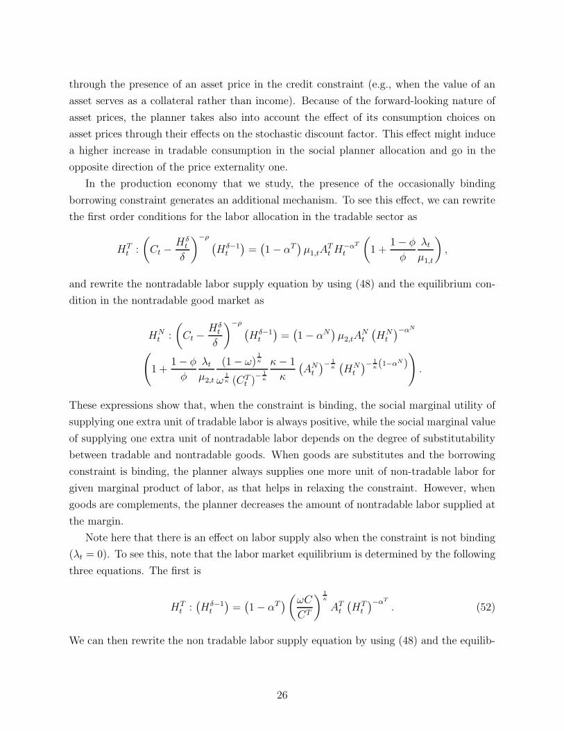
In the production economy that we study, the presence of the occasionally binding
borrowing constraint generates an additional mechanism. To see this effect, we can rewrite
the first order conditions for the labor allocation in the tradable sector as
HTt :
(Ct − Hδ
t
δ
)−ρ (Hδ−1
t
)=(1− αT
)μ1,tA
Tt H
−αT
t
(1 +
1− φ
φ
λt
μ1,t
),
and rewrite the nontradable labor supply equation by using (48) and the equilibrium con-
dition in the nontradable good market as
HNt :
(Ct − Hδ
t
δ
)−ρ (Hδ−1
t
)=(1− αN
)μ2,tA
Nt
(HN
t
)−αN
(1 +
1− φ
φ
λt
μ2,t
(1− ω)1κ
ω1κ (CT
t )− 1
κ
κ− 1
κ
(AN
t
)− 1κ(HN
t
)− 1κ(1−αN)
).
These expressions show that, when the constraint is binding, the social marginal utility of
supplying one extra unit of tradable labor is always positive, while the social marginal value
of supplying one extra unit of nontradable labor depends on the degree of substitutability
between tradable and nontradable goods. When goods are substitutes and the borrowing
constraint is binding, the planner always supplies one more unit of non-tradable labor for
given marginal product of labor, as that helps in relaxing the constraint. However, when
goods are complements, the planner decreases the amount of nontradable labor supplied at
the margin.
Note here that there is an effect on labor supply also when the constraint is not binding
(λt = 0). To see this, note that the labor market equilibrium is determined by the following
three equations. The first is
HTt :(Hδ−1
t
)=(1− αT
)(ωCCT
) 1κ
ATt
(HT
t
)−αT
. (52)
We can then rewrite the non tradable labor supply equation by using (48) and the equilib-
26

rium condition in the non-tradable good market to obtain:
HNt :(Hδ−1
t
)=(1− αN
)((1− ω)C
CN
) 1κ
ANt
(HN
t
)−αN
. (53)
where total labor supply is defined as
H = HT +HN . (54)
The system of equations given by (52), (53) and (54) determines total labor supply and the
sectoral allocation of labor for given CT , ATt and AN
t .
There are two effects in our production economy coming from the possibility that the
constraint might bind in the future. The first one is on total labor supply, while the second
is on the substitution between tradable and nontradable labor (intratemporal labor reallo-
cation effect). Both effects are induced by the fact that, in the social planner allocation,
current marginal utility of tradable consumption is higher compared to the competitive
equilibrium allocation. Higher current marginal utility of tradable consumption increases
the marginal utility of supplying one unit of labor today. As a result, in the social planner
allocation, labor supply is higher compared to the CE even when the constraint is not
binding. This effect alone can cause underborrowing in equilibrium.
The second effect depends on the intrasectoral labor allocation. Higher current marginal
utility of tradable consumption (i.e. μ1,t) in the SP implies that, for given total labor
supply, the planner will shift resources towards the tradable sector. This shift will reduce
the production and the consumption of non-tradable goods. When goods are complement
this reduction in the consumption of non-tradable consumption will also imply a reduction
in tradable consumption, and hence increasing the amount agents save in the SP allocation
relative to the CE allocation. The shift of labor towards tradable production then will tend
to strengthen overborrowing in the competitive allocation compared to the social planner
one.12 When goods are substitutes, the decline in nontradable consumption leads to an
12It is possible to see the effect on total labor supply by combining (51) and (50) when the constraint isnot binding to get
2
(Ct − Hδ
t
δ
)−ρ (Hδ−1
t
)=(1− αT
)μ1,tA
Tt H
−αT
t
⎛⎝1 +
(1− αN
)AN
t
(HN
t
)−αN
(1− αT )ATt H
−αT
t
μ2,t
μ1,t
⎞⎠
and note that when the constraint is not binding
μ2,t
μ1,t
=
⎛⎝(1− αN
)AN
t
(HN
t
)−αN
(1− αT )ATt H
−αT
t
⎞⎠
−1
27
increase in tradable consumption and as such to a decrease in the amount agents save in
the SP allocation compared to the CE allocation. Under substitutability sectoral allocation
of labor might induce underborrowing in the competitive equilibrium allocation. Note
finally that, in equilibrium, sectoral reallocation will have a feedback effect on total labor
supply by affecting wages in units of tradable goods.
In contrast to what we discussed for the competitive equilibrium, the specification of
the borrowing constraint has implications for the characterization of the social planner
allocation. While the production/labor supply choice are independent from the way the
constraint is specified (equations (52), (53) and (54) will remain the same), the intertem-
poral consumption pattern is affected by the way the planner manipulates the stochastic
discount factor when the borrowing constraint is specified in terms of asset prices.13 Con-
sider the following experiment in which the planner decreases future consumption while
increasing current consumption: by doing so, the planner increases the pricing kernel and
inflate asset prices. When the incentive of the planner to manipulate the intertemporal
consumption pattern dominates, marginal utility of tradable consumption today is lower
than in the competitive equilibrium the possibility of underborrowing arises.
In the papers by Bianchi and Mendoza (2010) and Korinek and Jeanne (2010) this
effect is not present despite the fact that they consider economies in which the borrowing
constraint depend on a key asset price. Bianchi and Mendoza (2010) do not have this effect
because to solve for the social planner problem they use the concept of conditional efficiency
(i.e. they assume that the asset price is determined by the asset price function that links
current asset price to the exogenous and endogenous state variables). By construction then
the planner cannot influence the intertemporal path of consumption. 14
4 Solution Methods
In this section we define the equilibria we consider and describe the global solution methods
that we use to compute them. We will present results for three different equilibria in
so that (Ct − Hδ
t
δ
)−ρ (Hδ−1
t
)=(1− αT
)μ1,tA
Tt H
−αT
t .
13The following reasoning is based on characterizing the constrained efficient social planner problem as inKehoe and Levine (1993) so that the equilibrium condition that determines asset prices in the competitiveallocation is taken as a constraint of the social planner problem.
14Using the concept of conditional efficiency has implications also for the behavior of the economy inthe binding region. When the amount of borrowing is constrained, conditional efficiency eliminates thepossibility that the planner can manipulate asset prices, forcing the social planner allocation to be closerto the competitive one.
28
Section 4. The first is the solution to the competitive equilibrium of the model. This is
the benchmark where there is no intervention on the part of a government. The second
is the social planners equilibrium. The third is the solution to the model with Ramsey
optimal policy. We will present optimal policies for different types of taxes. The solution
algorithm is the same in each case so here we explain only the solution for the case in
which the Ramsey planner has two instruments as an example. The solution of the cases in
which either of the alternative tax instruments are used individually are based on the same
algorithm.15 The competitive and social planner solution algorithms are those developed
by Benigno et al. (2010, 2011) so here we simply summarize them. The algorithm for the
solution of the optimal policy problem is a novel contribution of this paper, so we provide
extensive detail.
4.1 Competitive Equilibrium and Social Planner Solutions
The competitive equilibrium problem is defined by the first order conditions for the model
in Section 2. Following Benigno et al. (2010, 2011) the algorithm for the solution of the
competitive equilibrium is derived from Baxter (1990) and Coleman (1989), and involves
iterating on the functional equations that characterize a recursive competitive equilibrium
in the states(B,AT
). The key step is to transform the complementary slackness conditions
on the borrowing constraint into a set of nonlinear equations that can be solved using stan-
dard solvers (in particular, a modified Powell’s method). The key steps are to replace the
Lagrange multiplier, λt, with the expression max {λ∗t , 0}2 and to replace the complementary
slackness conditions
λt ≥ 0
Bt+1 +1− ϕ
ϕ
(AT
t
(HT
t
)1−αT+ PN
t A(HN
t
)1−αN)≥ 0
λt
(Bt+1 +
1− ϕ
ϕ
(AT
t
(HT
t
)1−αT + PNt A(HN
t
)1−αN))
= 0
with the single nonlinear equation
max {−λ∗t , 0}2 = Bt+1 +
1− ϕ
ϕ
(AT
t
(HT
t
)1−αT+ PN
t AN(HN
t
)1−αN).
15The code to solve the model is written in Fortran95 and available upon request. The optimal policyproblem is particularly sensitive to parameters and initial conditions, and there is no guarantee made thatthe programs work for parameter settings not considered explicitly here.
29
We then guess a function ηt+1 = Gη
(Bt+1, A
Tt+1
)and solve for
{λ∗t , ηt, Bt+1, C
Tt , C
Nt , HT
t , HNt , PN
t
}at each value for
(Bt, A
Tt
). This solution is used to update the Gη function to convergence.
Note that if the constraint binds, λ∗t > 0 so that max {−λ∗
t , 0}2 = 0.16
Given the solution for the equilibrium decision rules, we can compute the equilibrium
value of lifetime utility by solving the functional equation
V(Bt, A
Tt
)=
1
1− ρ
((ω
1κ
(CT
t
)κ−1κ + (1− ω)
1κ(CN
t
)κ−1κ
) κκ−1 − 1
δ
(HT
t +HNt
)δ)1−ρ
+
βE[V(Bt+1,
(AT
t+1
)) |ATt
];
this equation defines a contraction mapping and thus has a unique solution.
As in Benigno et al. (2010, 2011) to solve for the social planning equilibrium we set up
a standard dynamic programming problem
V SP(Bt, A
Tt
)= max
CT ,CN ,HT ,HN ,B′
1
1− ρ
((ω
1κ
(CT
t
)κ−1κ + (1− ω)
1κ(CN
t
)κ−1κ
) κκ−1 − 1
δ
(HT
t +HNt
)δ)1−ρ
+
βE[V SP
(Bt+1, A
Tt+1
) |ATt
]subject to the resource constraints, the borrowing constraint, and the marginal condition
that determines PN :
CTt = (1 + r)Bt + AT
t
(HT
t
)1−αT −Bt+1
CNt = AN
(HN
t
)1−αN
Bt+1 ≥ −1− ϕ
ϕ
(AT
t
(HT
t
)1−αT + PNt AN
(HN
t
)1−αN)
PNt =
(1− ω
ω
) 1κ(CN
t
CTt
)− 1κ
.
We approximate the function V SP using cubic splines, and solve the maximization using fea-
sible sequential quadratic programming. This functional equation also defines a contraction
mapping, so the planning solution is unique.
4.2 Optimal Policy Solution
The optimal policy solution assumes no commitment on the part of the policymaker. As an
example we describe the solution for optimal debt and non-tradable consumption taxation.
16Note also that λt = max {λ∗t , 0}2 ≥ 0, max {−λ∗
t , 0}2 ≥ 0, and max {λ∗t , 0}2 max {−λ∗
t , 0}2 = 0 so thecomplementary slackness conditions are satisfied. See Garcia and Zangwill (1981) for details.
30
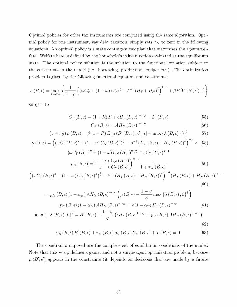
Optimal policies for other tax instruments are computed using the same algorithm. Opti-
mal policy for one instrument, say debt taxation, simply sets τN to zero in the following
equations. An optimal policy is a state contingent tax plan that maximizes the agents wel-
fare. Welfare here is defined by the household’s value function evaluated at the equilibrium
state. The optimal policy solution is the solution to the functional equation subject to
the constraints in the model (i.e. borrowing, production, budget etc.). The optimization
problem is given by the following functional equation and constraints:
V (B, ε) = maxτB ,τN
{1
1− ρ
((ωCκ
T + (1− ω)CκN)
1κ − δ−1 (HT +HN)
δ)1−ρ
+ βE [V (B′, ε′) |ε]}
subject to
CT (B, ε) = (1 +R)B + εHT (B, ε)1−αT − B′ (B, ε) (55)
CN (B, ε) = AHN (B, ε)1−αN (56)
(1 + τB)μ (B, ε) = β (1 +R)E [μ (B′ (B, ε) , ε′) |ε] + max {λ (B, ε) , 0}2 (57)
μ (B, ε) =((ωCT (B, ε)κ + (1− ω)CN (B, ε)κ)
1κ − δ−1 (HT (B, ε) +HN (B, ε))δ
)−ρ
× (58)
(ωCT (B, ε)κ + (1− ω)CN (B, ε)κ)1κ−1
ωCT (B, ε)κ−1
pN (B, ε) =1− ω
ω
(CN (B, ε)
CT (B, ε)
)κ−11
1 + τN (B, ε)(59)(
(ωCT (B, ε)κ + (1− ω)CN (B, ε)κ)1κ − δ−1 (HT (B, ε) +HN (B, ε))δ
)−ρ
(HT (B, ε) +HN (B, ε))δ−1
(60)
= pN (B, ε) (1− αN)AHN (B, ε)−αN
(μ (B, ε) +
1− ϕ
ϕmax {λ (B, ε) , 0}2
)pN (B, ε) (1− αN)AHN (B, ε)−αN = ε (1− αT )HT (B, ε)−αT (61)
max {−λ (B, ε) , 0}2 = B′ (B, ε) +1− ϕ
ϕ
(εHT (B, ε)1−αT + pN (B, ε)AHN (B, ε)1−αN
)(62)
τB (B, ε)B′ (B, ε) + τN (B, ε) pN (B, ε)CN (B, ε) + T (B, ε) = 0. (63)
The constraints imposed are the complete set of equilibrium conditions of the model.
Note that this setup defines a game, and not a single-agent optimization problem, because
μ (B′, ε′) appears in the constraints (it depends on decisions that are made by a future
31
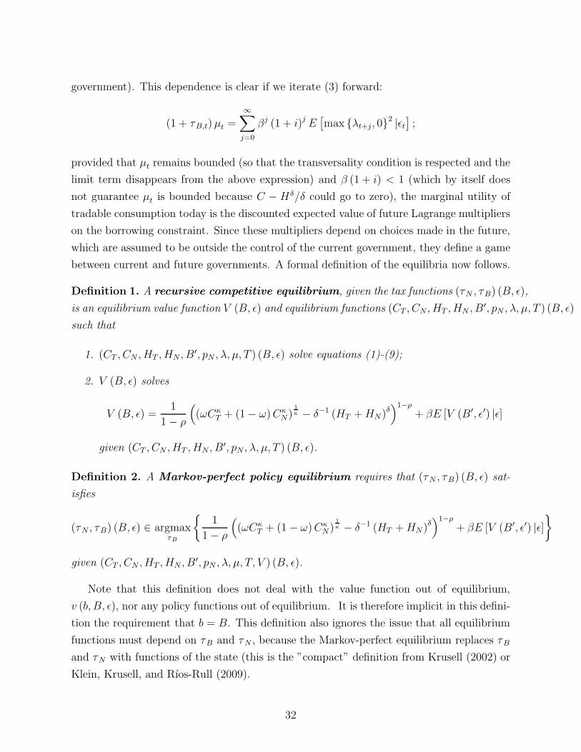
government). This dependence is clear if we iterate (3) forward:
(1 + τB,t)μt =
∞∑j=0
βj (1 + i)j E[max {λt+j, 0}2 |εt
];
provided that μt remains bounded (so that the transversality condition is respected and the
limit term disappears from the above expression) and β (1 + i) < 1 (which by itself does
not guarantee μt is bounded because C − Hδ/δ could go to zero), the marginal utility of
tradable consumption today is the discounted expected value of future Lagrange multipliers
on the borrowing constraint. Since these multipliers depend on choices made in the future,
which are assumed to be outside the control of the current government, they define a game
between current and future governments. A formal definition of the equilibria now follows.
Definition 1. A recursive competitive equilibrium, given the tax functions (τN , τB) (B, ε),
is an equilibrium value function V (B, ε) and equilibrium functions (CT , CN , HT , HN , B′, pN , λ, μ, T ) (B, ε)
such that
1. (CT , CN , HT , HN , B′, pN , λ, μ, T ) (B, ε) solve equations (1)-(9);
2. V (B, ε) solves
V (B, ε) =1
1− ρ
((ωCκ
T + (1− ω)CκN)
1κ − δ−1 (HT +HN)
δ)1−ρ
+ βE [V (B′, ε′) |ε]
given (CT , CN , HT , HN , B′, pN , λ, μ, T ) (B, ε).
Definition 2. A Markov-perfect policy equilibrium requires that (τN , τB) (B, ε) sat-
isfies
(τN , τB) (B, ε) ∈ argmaxτB
{1
1− ρ
((ωCκ
T + (1− ω)CκN)
1κ − δ−1 (HT +HN)
δ)1−ρ
+ βE [V (B′, ε′) |ε]}
given (CT , CN , HT , HN , B′, pN , λ, μ, T, V ) (B, ε).
Note that this definition does not deal with the value function out of equilibrium,
v (b, B, ε), nor any policy functions out of equilibrium. It is therefore implicit in this defini-
tion the requirement that b = B. This definition also ignores the issue that all equilibrium
functions must depend on τB and τN , because the Markov-perfect equilibrium replaces τB
and τN with functions of the state (this is the ”compact” definition from Krusell (2002) or
Klein, Krusell, and Rıos-Rull (2009).
32
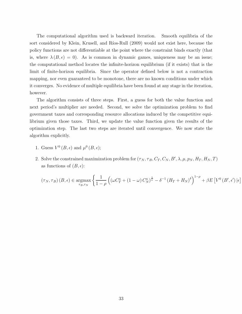
The computational algorithm used is backward iteration. Smooth equilibria of the
sort considered by Klein, Krusell, and Rıos-Rull (2009) would not exist here, because the
policy functions are not differentiable at the point where the constraint binds exactly (that
is, where λ (B, ε) = 0). As is common in dynamic games, uniqueness may be an issue;
the computational method locates the infinite-horizon equilibrium (if it exists) that is the
limit of finite-horizon equilibria. Since the operator defined below is not a contraction
mapping, nor even guaranteed to be monotone, there are no known conditions under which
it converges. No evidence of multiple equilibria have been found at any stage in the iteration,
however.
The algorithm consists of three steps. First, a guess for both the value function and
next period’s multiplier are needed. Second, we solve the optimization problem to find
government taxes and corresponding resource allocations induced by the competitive equi-
librium given those taxes. Third, we update the value function given the results of the
optimization step. The last two steps are iterated until convergence. We now state the
algorithm explicitly.
1. Guess V 0 (B, ε) and μ0 (B, ε);
2. Solve the constrained maximization problem for (τN , τB, CT , CN , B′, λ, μ, pN , HT , HN , T )
as functions of (B, ε):
(τN , τB) (B, ε) ∈ argmaxτB ,τN
{1
1− ρ
((ωCκ
T + (1− ω)CκN)
1κ − δ−1 (HT +HN)
δ)1−ρ
+ βE[V 0 (B′, ε′) |ε]}
33

subject to
CT (B, ε) = (1 +R)B + εHT (B, ε)1−αT −B′ (B, ε) (64)
CN (B, ε) = AHN (B, ε)1−αN (65)
(1 + τB)μ1 (B, ε) = β (1 +R)E
[μ0 (B′ (B, ε) , ε′) |ε]+max {λ (B, ε) , 0}2 (66)
μ1 (B, ε) =((ωCT (B, ε)κ + (1− ω)CN (B, ε)κ)
1κ − δ−1 (HT (B, ε) +HN (B, ε))δ
)−ρ
×(67)
(ωCT (B, ε)κ + (1− ω)CN (B, ε)κ)1κ−1
ωCT (B, ε)κ−1
pN (B, ε) =1− ω
ω
(CN (B, ε)
CT (B, ε)
)κ−11
1 + τN (B, ε)(68)(
(ωCT (B, ε)κ + (1− ω)CN (B, ε)κ)1κ − δ−1 (HT (B, ε) +HN (B, ε))δ
)−ρ
(HT (B, ε) +HN (B, ε))δ−1
(69)
= pN (B, ε) (1− αN )AHN (B, ε)−αN
(μ1 (B, ε) +
1− ϕ
ϕmax {λ (B, ε) , 0}2
)pN (B, ε) (1− αN )AHN (B, ε)−αN = ε (1− αT )HT (B, ε)−αT (70)
max {−λ (B, ε) , 0}2 = B′ (B, ε) +1− ϕ
ϕ
(εHT (B, ε)1−αT + pN (B, ε)AHN (B, ε)1−αN
)(71)
τB (B, ε)B′ (B, ε) + τN (B, ε) pN (B, ε)CN (B, ε) + T (B, ε) = 0. (72)
Note here that, the program also imposes nonnegativity constraints on those variables
that require them (consumption, labor supply, prices). The constraint that the
argument of the utility function is positive is imposed explicitly to avoid convergence
issues:
(ωCκT + (1− ω)Cκ
N)1κ − δ−1 (HT +HN)
δ > 0.
There is a potential complication: since the constraint set is not generally convex, the
value function may not be concave (or even continuous). As a result, the program is
solved using a number of methods (a Nelder-Mead search method, a feasible sequential
quadratic programming approach FQSP, and a global search method called GLOBAL)
designed to ensure we achieve a global maximum; depending on the instruments used,
one or more of these approaches may fail. The failure of concavity also implies that
there may exist multiple solutions and/or the decisions rules may not be continuous.
The feasible sequential quadratic programming approach has proven to be the fastest
and converges in all cases considered to date.
34
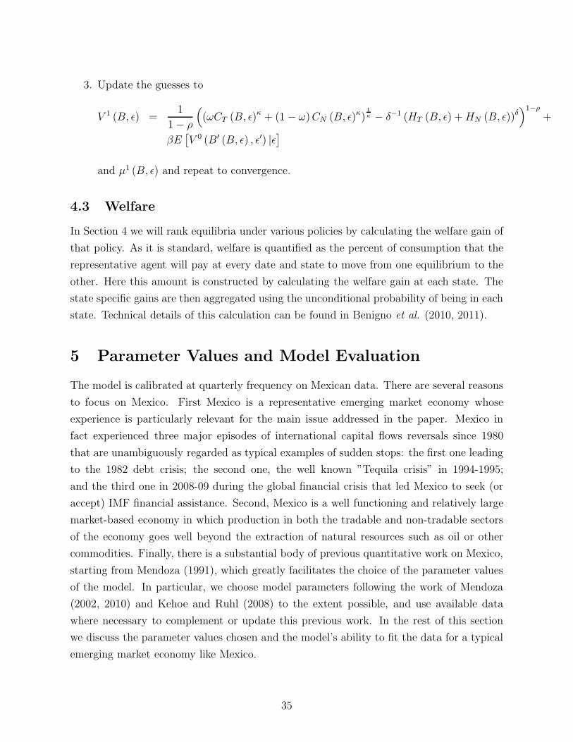
3. Update the guesses to
V 1 (B, ε) =1
1− ρ
((ωCT (B, ε)κ + (1− ω)CN (B, ε)κ)
1κ − δ−1 (HT (B, ε) +HN (B, ε))δ
)1−ρ
+
βE[V 0 (B′ (B, ε) , ε′) |ε]
and μ1 (B, ε) and repeat to convergence.
4.3 Welfare
In Section 4 we will rank equilibria under various policies by calculating the welfare gain of
that policy. As it is standard, welfare is quantified as the percent of consumption that the
representative agent will pay at every date and state to move from one equilibrium to the
other. Here this amount is constructed by calculating the welfare gain at each state. The
state specific gains are then aggregated using the unconditional probability of being in each
state. Technical details of this calculation can be found in Benigno et al. (2010, 2011).
5 Parameter Values and Model Evaluation
The model is calibrated at quarterly frequency on Mexican data. There are several reasons
to focus on Mexico. First Mexico is a representative emerging market economy whose
experience is particularly relevant for the main issue addressed in the paper. Mexico in
fact experienced three major episodes of international capital flows reversals since 1980
that are unambiguously regarded as typical examples of sudden stops: the first one leading
to the 1982 debt crisis; the second one, the well known ”Tequila crisis” in 1994-1995;
and the third one in 2008-09 during the global financial crisis that led Mexico to seek (or
accept) IMF financial assistance. Second, Mexico is a well functioning and relatively large
market-based economy in which production in both the tradable and non-tradable sectors
of the economy goes well beyond the extraction of natural resources such as oil or other
commodities. Finally, there is a substantial body of previous quantitative work on Mexico,
starting from Mendoza (1991), which greatly facilitates the choice of the parameter values
of the model. In particular, we choose model parameters following the work of Mendoza
(2002, 2010) and Kehoe and Ruhl (2008) to the extent possible, and use available data
where necessary to complement or update this previous work. In the rest of this section
we discuss the parameter values chosen and the model’s ability to fit the data for a typical
emerging market economy like Mexico.
35
5.1 Parameter Values
The specific set of parameter values that we use in our baseline calibration are reported in
Table 1. The inverse of the elasticity of intertemporal substitution is set to a standard value
of ρ = 2, like in Mendoza (2002, 2010). We set then the world interest rate to i = 0.01587,
which yields an annual real rate of interest of about 6.5 percent like in Mendoza (2002):
a value that is between the 5 percent of Kehoe and Ruhl (2008) and the 8.6 percent of
Mendoza (2010).
The elasticity of intratemporal substitution in consumption between tradables and non-
tradables is an important parameter in the analysis as we discussed in the previous section.
There is significant consensus in the literature on its value. We follow Ostry and Reinhart
(1992), who estimates a value of κ = 0.760 for developing countries. This is a conservative
assumption compared to the value of 0.5 used by Kehoe and Ruhl (2008) and closer to the
one assumed for an advanced, more closed economy like the United States.
Estimates of the wage elasticity of labor supply in Mexico are uncertain at best (Men-
doza, 2002 and 2010). We set the value of δ = 1.75, close to the value of 1.84 adopted by
Mendoza (2010).17
The labor share of income, (1 − αT ) and (1 − αN) is set to 0.66 in both tradable and
nontradable sectors: a standard value, close to that used by Mendoza (2002), and consistent
with empirical evidence on the aggregate share of labor income in GDP in the household
survey of Garcia-Verdu (2005).
The shock to tradable total factor productivity specified as
log(AT
t
)= ρA log
(AT
t−1
)+ εt,
where εt is an iid N(0, σ2A) innovation. The parameters of this process are set to ρA = 0.537
and σA = 0.0134 which are the first autocorrelation and the standard deviation of aggregate
total factor productivity reported by Mendoza (2010). Both the average value of AT and
the constant AN are set to one.
The remaining three model parameters — the share of tradable consumption in the
consumption basket (ω), the credit constraint parameter (φ), and the discount factor (β)
— are set by iterating on a routine that minimizes the sum of squared differences between
the moments in the ergodic distribution of the competitive equilibrium of the model and
three data targets. The data targets are a CN/CT ratio of 1.643, a 35 percent debt-to-GDP
17The value of this parameter is 2 in Benigno et al. (2011). The higher elasticity used here allows usto replicate the higher volatility of consumption growth relative to income growth common in emergingmarket economies.
36
ratio, and an unconditional probability of a sudden stop equal to 2 percent per quarter.
This CN/CT ratio is the value implied by the following ratios estimated by Mendoza (2002):
Y T/Y N =0.648, CT/Y T =0.665, and CN/Y N =0.708 as in Mendoza (2002).18 The debt-
to-GDP target is Mexico’s average net foreign asset to annual GDP ratio, from 1970 to
2008, in the updated version of the Lane and Milesi-Ferretti (2006) data set.
The target for the unconditional probability of a sudden stop is more difficult to pin
down. Despite a significant body of empirical work on identifying sudden stops in emerging
markets to describe the macroeconomic dynamics around these events, there is no consensus
in the literature on how to define sudden stops empirically, and hence no accepted measure of
the unconditional probability of these events. By focusing on Mexico, we can pin down this
target simply and unambiguously, measuring it as the relative frequency, on a quarterly
basis, of Mexico’s sudden stops years over the period 1975-2010. We assume that, as
generally accepted, 1982, 1995, and 2009 were sudden stop years for Mexico. The resulting
2 percent is very close to the 1.9 percent implied by the empirical analysis of Jeanne and
Ranciere (2010) over the period 1975-2003, who use an “absolute” definition of sudden stops
as current account reversals larger than 5 percent of GDP. Our number is also similar to the
2.2 percent value implied by Calvo, Izquierdo, and Mejia (2008) for the period 1990-2004,
based on a “relative” definition of sudden stops as current account reversals larger than
two standard deviations. The 2 percent value, however, is at the low end of the range of
values estimated in these studies by pooling data for the whole sample of emerging markets
considered.
In order to contrast Mexico data with model outcomes during sudden stop episodes,
consistent with both the model and the empirical literature above, we define a sudden stop
in the model as an event in which: (a) λt > 0 (i.e. the international borrowing constraint
is binding) and (b) (Bt+1−Bt) > 2σ(Bt+1−Bt) (i.e. the current account or changes in the
net foreign asset position in a given period exceed two times its standard deviation). The
first criterion is a purely model based definition sudden stop. The second criterion allows
us to consider only model events in which there are large current account reversals, in line
with the aforementioned empirical literature.19 20
18Ratios computed with updated data are essentially the same. As we evaluate the model’s ability toreplicate the 1995 Tequila crisis we use the exact values reported by Mendoza (2002).
19The definition of sudden stop typically used in the empirical literature focuses on large capital flowsreversals because some smaller ones may be due to terms of trade changes or other factors Jeanne andRanciere (forthcoming), for instance, excludes commodity importers and oil producers, while Calvo et al.(DATE) add other criteria to the second one we use above.
20Note that national accounts data typically have a trend, and hence the empirical literature focuseschanges in the current account, or the first difference of the capital flows. As our model has no trendgrowth and the data are in percent deviation from HP filter, we focus on the current account rather thanits change. We obtain similar results when we define the sudden stop with respect to changes in the current
37

With the targets above we obtain ω = 0.3526, β = 0.9717, and φ = 0.415. The implied
value of ω is slightly higher than in Mendoza (2002) and slightly lower than targeted by
Kehoe and Ruhl (2008). The implied annual value of β is yield an annual discount factor of
0.8915, only slightly lower than in Kehoe and Ruhl (2008).21 The implied value of φ is lower
than in Mendoza (2002), who however calibrates it to the deterministic steady state of the
model, and there are no standard benchmarks for this model parameter in the literature.
5.2 Model Evaluation
The class of models we study is potentially capable of describing well both the cycle and
the crisis periods of an emerging market economy like Mexico (Mendoza 2010). However,
in our implementation of the model, we shut down a number of shocks used in other work
and focus on the mechanisms driving our policy results. With our one shock we clearly
cannot match all the moments of the data that this class of models is capable of replicating.
Nonetheless, it is useful to see how well our one shock model does do in describing both the
business cycle and the dynamics around a typical sudden stop event, as the first exercise is
standard and helps to understand the findings in the second one.
To conduct this comparison we use the variable as defined in Table 2. All data variables
are reported in percent deviations from the HP-filter trend (over the 1993Q1-2007Q4 period)
except the current account, which is reported as a share of GDP. All model variables are
reported in percent deviation from ergodic mean except the current account that is reported,
as in the data, as a share of GDP. To calculate model moments we simulate the model for
1,000,000 time periods, and retain the final 10,000 simulation periods to calculate moments
and identify sudden stop events.
Table 3 reports data and simulated second moments. Despite its simplicity, the model
describes the data reasonably well except for the behavior of the tradable GDP that is
counterfactual because of the behavior of labor supply when the constraint is binding in
our model economy. As we can see, once we normalize all standard deviations relative
to GDP in units of tradable goods (as in Bianchi, 2010), the model roughly matches the
ranking of the data volatilities consistent with the results in Mendoza (2002), despite the
fact that the model has only one shock. In particular, the model generates consumption
volatility that is almost as high as GDP volatility and a current account that is less volatile
that aggregate GDP or its components. The model however produces higher relative price
account.21This value is not comparable to the one assumed by Mendoza (2002) as he uses an endogenous discount
factor specification. In our model, the presence of the borrowing constraint removes the necessity tointroduce any device to induce a stationary ergodic distribution of foreign borrowing.
38
volatility and too low tradable GDP volatility relative to the data (i.e. relative to GDP
volatility).22 Like in the data, all model variables are similarly persistent, but less than
in the data (especially for the relative price on nontradable goods and tradable GDP). All
correlations with GDP except the relative price one are also all roughly consistent with
the data. The correlation between CA and GDP is positive contrary to what we observe
in the data. This is because, as calibrated to Mexican data, the constraint does not alter
consumption smoothing enough in the ergodic distribution of our model to generate such
negative correlation.23 Note in addition that, the correlation between CA and net income
(defined as GDP minus investment and government expenditure, and hence closer to our
model definition) may be either slightly positive or zero in the average emerging market
economy (Luo, Nie, and Young 2010). Indeed, as it is well known (Backus, Kehoe, and
Kydland 1994), a model with investment would generate a negative correlation.
Similar strengths and weaknesses emerge by comparing the macroeconomic dynamics
around a typical sudden stop event. For this comparison, we focus on the 1995 Tequila crisis,
the same episode studied by Kehoe and Ruhl (2008) and Mendoza (2010). Specifically,
Figure 1 compares the model and the Mexican data for key variables four quarters before
and after 1995Q1, where the model variables are average across the identified sudden stop
episodes, four periods before and four periods after our sudden stop definition is initially
met.24
As we can see from Figure 1, the model qualitatively reproduces the large declines in
expenditure on consumption and output (both expressed in units of tradable goods), and
the relative price of tradable during the 1995 Tequila crisis in Mexico. However in the
model this relative price decline is less persistent than in the data. Similarly, qualitatively,
non tradable output and expenditure on non-tradable consumption measured in units of
tradables are described relatively well by the model. The same lack of persistence charac-
terizes all model variables that generally recover much faster than in the data. We note
also that consumption expenditure falls much more than output in our model economy
since, in the model, tradable output increases in sudden stop. Consistent with the data,
tradable GDP also starts to fall sharply before the sudden stops, but it increases during
the sudden stop period, counterfactually. As a result, tradable consumption falls much less
22Note that, using data up to 2007, as we do, the absolute value of consumption volatility in the data ismuch lower than reported by Mendoza (2002), and hence much closer to GDP volatility.
23For instance, Bianchi (2010) calibrates to Argentine data and obtains a negative correlation by usingthe combination of a high shock variance and a low discount factor.
24As it is evident in the capital flow data (not reported), while capital flows into Mexico started to revertin the fourth quarter of 1994, they were initially accommodated by a very large decrease in official reservesthat eventually lead to collapse of the fixed exchange rate regime in December 1994. As a result, the currentaccount started to revert only in 1995Q1.
39
than nontradable consumption, while in the data the opposite occurs.
Quantitatively, however, the model produces a sudden stop dynamics of amplitude
roughly one-order of magnitude smaller than in the data. This occurs for two reasons. First,
as we noted above, the model is too simple to provide an accurate quantitative account of
the data: in particular we limit ourselves to only one shock in tradable productivity while
other shocks (for example foreign interest rate shocks) might have contributed in amplifying
the dynamic of the economy during sudden stop. Second, and more importantly, the model
counterfactually predicts an increase in total employment at the sudden stop, driven by a
sharp increase in labor supply and fall in the real wage (not reported).
As Kehoe and Ruhl (2008) discuss there are three ways to generate a falling employ-
ment in the model: a friction in the labor mobility across sectors, variable capital utilization,
and a working capital constraint, but none produces satisfactory account of labor market
dynamics during the Tequila crisis in their model. In addition, in our model they pose
additional complications. Imperfect labor mobility and variable capital utilization intro-
duce an additional state variable. But, as we noted earlier, the comparison between the
competitive and the social planner allocation that is the focus of the paper constrains the
number of endogenous state variable that can feature in our model. A working capital
constraint could produce falling output, but would complicates the specification of the bor-
rowing constraint. In addition a working capital constraint would generate output falling
at the sudden stop, but would not alter the underlying mechanism at work in the region in
which we examine inefficient borrowing (i.e. during tranquil times) so that our discussion
on the role of macro-prudential policies would be robust to this change. For these reasons,
at first pass, we prefer to keep the model simple.
6 Optimal Policies in A Two-Goods, Two-Sectors Pro-
duction Economy
In this section we study optimal policies numerically. We first consider two optimal policy
problems in which the Ramsey planner has one instrument only, either exchange rate policy
(i.e., a tax on non-tradable consumption, τNt ) ) or direct controls on capital flows (a tax on
debt, τBt ) as in Section 2.25 As neither of these two instruments alone achieves constrained
efficiency, we also consider the case in which the planner uses both instruments at the same
time.
25Results for optimal policy with a tax on tradable consumption are not reported to conserve space butare available from the authors on request. They are consistent with the analysis in Section 2, and confirmthat, in our set up, exchange rate policy could be analyzed considering either of these two tax instruments.
40
6.1 Optimal Policies with One Instrument
Figure 2 reports the decision rules for each of the policy instrument considered, τNt or τBt
(where a positive value is a tax and a negative value is a subsidy). Figure 3 reports the
decision rules for key endogenous variables under these two alternative optimal policies
(OPs), as well as in the competitive equilibrium (CE) and the social planner allocation of
the economy (SP) for comparison. Figure 4 reports the ergodic distribution of debt in these
four different cases. Tables 4, 5 and 6 report the following: the mean and the standard
deviation of debt, the real exchange rate (the relative price of non-tradable goods in the
model), consumption, and the tax rates; the unconditional probability of a financial crisis;
and the welfare gain compared to the CE equilibrium for all the alternative policy regimes,
respectively.
If the Ramsey planner has only one instrument, the optimal intervention is a tax before
the constraint binds and a subsidy while the constraint binds strictly, regardless of the
instrument used. Thus, the optimal Ramsey policy (OP) is non linear and has a precau-
tionary component regardless of the instrument used. Both type of interventions can be
interpreted as ”leaning against the wind” kind of policies in normal times, either against
the real exchange rate or capital flows, and ”bail outs” in crisis times, either in the do-
mestic good market or the international capital market.26 But, unlike the endowment case
analyzed in Section 2, in the case of a production economy, neither exchange rate policy
nor controls on capital flows can achieve constrained efficiency (i.e., the SP allocation in
Figure 3).
Notwithstanding these similarities, there are important differences in the effects and
the working of the two optimal policies. Relative to the CE, exchange rate policy allows
for a more appreciated but less volatile exchange rate than the control on capital flows
(Figure 3 and Table 4), more and more volatile borrowing (Figure 4 and Table 5), and
much higher welfare (both overall and during periods of financial crisis as illustrated by
Table 6). Welfare is higher because the average level of consumption is higher with exchange
rate policy. This increase occurs despite the fact that, in the OP regime with exchange rate
policy as an instrument, the probability of financial crises is much higher than in the OP
regime with controls on capital flows (albeit smaller than in the CE). Note also that the
welfare gains from OP with capital controls are not only one order of magnitude smaller
than those with exchange rate policy, but also arise primarily in normal times, while with
exchange rate policy they arise mostly in crisis times.
26Note that, both type of interventions in crisis times can potentially be financed by the governmentintervention (in opposite direction) in normal times.
41
From a quantitative perspective, the exchange rate intervention rule computed requires
a tax on non-tradable consumption of about 5 percent per quarter on average, inducing
only a small exchange rate appreciation relative to the CE equilibrium and similar volatility
(Table 4). In contrast, the capital control rule computed requires a much smaller tax on
debt of about 0.2 percent per quarter on average, but produces a more volatile exchange
rate at the same average level of the CE. Given that the average size of the interventions
in crisis states are smaller or equal to the size of the intervention in normal times (not
reported), and that the economy spends only a very small fraction of the time in crises
states, the cost of intervening in crisis states can be easily financed by the tax proceeds in
normal times under both policy regimes.
6.2 Optimal Policy with Two Instruments
As neither of the two policies considered can replicate the constrained efficient outcome, we
also examine the optimal mix of the two policy instruments. Figure 5 reports the decision
rules for each of the policy instrument considered, τNt and τBt , when used one at a time or
together. Figure 3 reports the decision rules for key endogenous variables in all previous
cases as well as in the new case in which OP is implemented using both exchange rate
policy and controls on capital flows. Table 4, 5 and 6 report the relevant statistics also for
this additional case.
If the Ramsey planner has both a consumption tax and a tax on debt as instruments,
the optimal intervention is no intervention in normal times and a tax on debt combined
with a subsidy on non-tradable consumption during financial crises (Figure 5). Thus, in
states of the world in which the constraint is not binding the optimal policy is “no action”.
This result means that there is no precautionary motive in the optimal policy related to
the presence of the borrowing constraint if there is enough instruments to intervene more
effectively when a crisis strikes. Note that, as we illustrated in Section 3, the pecuniary
externality that justifies policy intervention, is active when the constraint binds or it is
expected to bind in the future. Therefore, if OP is more effective in intervening during a
crisis, there is no need to intervene before it strikes because the cost of the tax distortions
is larger than the benefit from using them in normal times.Note also that the average size
of the intervention, for both instruments, is much larger in the OP with two instruments
than the case in which there is only one instrument. One intuition for this result is that as
each of this instrument push the economy in a different direction, when both are used, both
can be used more aggressively without facing a trade off in their effectiveness on different
margins. With two instruments, it is conceivable that the proceeds from taxing debt might
42
finance part of the subsidy to finance the subsidy.
With two instruments, welfare is much higher than with exchange rate policy or capital
controls alone, but yet it does not achieve the level associated with constrained efficiency by
the SP allocation (Table 6).27 Debt is also higher (but less volatile) than the case in which
there is only exchange rate policy (Table 5). The real exchange rate is more appreciated
and even less volatile than the exchange rate policy case.
7 Conclusions
In this paper we study optimal policy for macro-financial stability in an small open economy
in which a foreign borrowing constraint binds only occasionally and a financial crisis is an
endogenous event. In this environment, scope for policy before and during financial crises
arises because of a pecuniary externality stemming from the presence of a key relative price
in the borrowing constraint. In an endowment version of our economy (i.e., Bianchi 2011),
if the policy maker has only one instrument, we find analytically that (i) a tax or subsidy
on consumption (i.e., exchange rate policy) can achieve the first best allocation, while a
tax or subsidy on foreign borrowing (i.e., a capital control) can only achieve a second best
allocation; (ii) Ramsey optimal policy under discretion is the same as under commitment
and achieves the same allocation selected by a social planner that is not constrained by the
behavior of the private sector. In a production version of our economy (i.e., Benigno et al.
2011), we find numerically that, (iii) if the Ramsey planner has only one instrument, the
optimal intervention is a prudential tax regardless of the instrument used. However (iv),
if the Ramsey planner has both a consumption tax and a tax on debt as instruments, the
optimal intervention is a tax on debt and a subsidy on consumption during financial crises
and no intervention in normal times. Finally, we also find numerically that (v) exchange rate
policy dominates controls on capital flows if the Ramsey planner has only one instrument,
but neither achieves the second best constrained efficient allocation selected by a social
planner.
Overall, these results suggest that, if the there is only one instrument available to deal
with multiple distortions, intervening on the exchange rate may be a superior way to enact
optimal policy taking macro-financial stability considerations into account. Note that both
policy rules entails a ”leaning against the wind” component in normal times and a ”bailout”
component in crisis times (an exchange rate defense in the case of exchange rate policy and
27There are three distorted margins in this economy and only two instruments. Adding a tax on laborincome, which enters the third margin, has little effect and still does not achieve constrained efficiency; thecommitment issue thus appears to be critical.
43

a subsidy element to foreign borrowing with capital controls). The leaning against the wind
components in normal times may potentially finance the bailout components in crisis times.
An important methodological contribution of the paper is the development of compu-
tational algorithms to solve optimal policy problems in environments with constraints that
bind on occasion.
44
References
[1] Adam, K. and R.M. Billi, (2006), ”Optimal Monetary Policy under Commitment witha Zero Bound on Nominal Interest Rates,” Journal of Money, Credit and Banking38(7), pp. 1877-1905.
[2] Adam, K. and R.M. Billi (2007), ”Discretionary Monetary Policy and the Zero LowerBound on Nominal Interest Rates,” Journal of Monetary Economics 54(3), pp. 728-752.
[3] Aghion, P. and P. Bacchetta and A. Banerjee (2004), “Financial Development and theInstability of Open Economies,” Journal of Monetary Economics 51(6), pp. 1077-1106.
[4] Arellano, C. and E. Mendoza (2003), “Credit Frictions and ’Sudden Stops’ in SmallOpen Economies: An Equilibrium Business Cycle Framework for Emerging MarketsCrises,” in S. Altug, J. Chadha, and C. Nolan (eds.), Dynamic Macroeconomic Anal-ysis: Theory and Policy in General Equilibrium, Cambridge U. Press, 2003.
[5] Arnott, R. and B. Greenwald and J. E. Stiglitz (1994), “Information and EconomicEfficiency,” Information Economics and Policy 6(1), pp. 77-82.
[6] Baxter, M. (1991), “Approximating Suboptimal Dynamic Equilibria: An Euler Equa-tion Approach,” Journal of Monetary Economics 28(2), pp. 173-200.
[7] Backus, D. and P.J. Kehoe and F.E. Kydland (1993), “International Business Cycles:Theory and Evidence,” NBER Working Papers 4493, National Bureau of EconomicResearch.
[8] Benigno, G. and H. Chen and C. Otrok and A. Rebucci and E. Young (2010), “Revis-iting Overborrowing and its Policy Implications,” CEPR DP. No. 7872.
[9] Benigno, G. and H. Chen and C. Otrok and A. Rebucci and E. Young (2011), “FinancialCrises and Macro-Prudential Policies,” CEPR DP. 8175
[10] Bianchi, J. (2009), “Overborrowing and Systemic Externalities in the Business Cycle,”American Economic Review, forthcoming.
[11] Bianchi J. and E. G. Mendoza (2010), “Overborrowing, Financial Crises and ’Macro-prudential’ Taxes,” NBER Working Papers 16091, National Bureau of Economic Re-search.
[12] Braggion, F., L.J. Christiano and J. Roldos (2007),“Optimal Monetary Policy in a‘Sudden Stop’,” NBER Working Paper 13254.
[13] Bordo, M.D and O. Jeanne (2002), “Monetary Policy and Asset Prices: Does ’BenignNeglect’ Make Sense?” International Finance, Blackwell Publishing, vol. 5(2), pp. 139-64.
[14] Caballero, R. J. (2010), “Sudden Financial Arrest,” IMF Economic Review, forthcom-ing.
[15] Caballero, R.J. and A. Krishnamurthy (2005), “Inflation Targeting and Sudden Stops,”in Bernanke, B.S. and M. Woodford (eds.), The Inflation-Targeting Debate, Universityof Chicago Press.
[16] Calvo, G.A. and A. Izquierdo and L.F. Mejıa (2008), “Systemic Sudden Stops: TheRelevance Of Balance-Sheet Effects And Financial Integration,” NBER Working Pa-pers 14026, National Bureau of Economic Research, Inc.
[17] Chari, V.V. and P. J. Kehoe (2009), “Bailouts, Time Inconsistency and Optimal Reg-ulation,” Working Paper, Federal Reserve Bank of Minneapolis.
[18] Caballero, R.J. and S. Panageas (2007), “A Global Equilibrium Model of Sudden Stopsand External Liquidity Management,” unpublished manuscript, MIT.
[19] Calvo, G.A. (1998), “Capital Flows and Capital-Markets Crises: The Simple Eco-nomics of sudden stops,” Journal of Applied Economics 1(1), pp. 35-54.
[20] Chari, V. V. and P.J. Kehoe (1999), “Optimal Fiscal and Monetary Policy,” NBERWorking Papers 6891.
[21] Christiano, L.J., C. Gust, and J. Roldos (2004), “Monetary Policy in a FinancialCrisis,” Journal of Economic Theory.
[22] Coleman, W.J., II (1991), “Equilibrium in a Production Economy with an IncomeTax,” Econometrica 59(4), pp. 1091-1104.
[23] Coleman, W.J., II (1997), “Equilibria in Distorted Infinite-Horizon Economies withCapital and Labor,” Journal of Economic Theory 72(2), pp. 446-61.
[24] Curdia, V. (2007), “Optimal Monetary Policy under sudden stops,” Federal ReserveBank of New York Staff Report No. 278.
[25] Devereux, M.B. and D. Poon (2004), “A Smple Model of Optimal Monetary Policywith Financial Constraints,” unpublished manuscript, UBC.
[26] Eaton, J. and M. Gersovitz (1981), “Debt with Potential Repudiation: Theoreticaland Empirical Analysis,” Review of Economic Studies 48(2), pp.289-309.
[27] Fernandez-Arias, E. and D. Lombardo (1998), “Private External Overborrowing inUndistorted Economies: Market Failure and Optimal Policy,” Working Paper No. 369,Inter-American Development Bank.
[28] Garcıa-Verdu, R. (2005), “Factor Shares from Household Survey Data,” Banco deMexico, Working Paper 2005-05.
[29] Greenwood, J. and Z. Hercowitz and G.W. Huffman (1988), “Investment, CapacityUtilization, and the Real Business Cycle,” American Economic Review 78(3), pp. 402-417.
[30] Greenwood, J. and G.W. Huffman (1995), “On the Existence of Nonoptimal Equilibriain Dynamic Stochastic Economies,” Journal of Economic Theory 65(2), pp. 611-623.
[31] Hevia, C. (2008), “Optimal Policy with Sudden Stops,” World Bank working paper.
[32] Jeanne, O. and A. Korinek (2010), “Excessive Volatility in Capital Flows: A PigouvianTaxation Approach,” American Economic Review 100(2), pp. 403-407.
[33] Jeanne, O. and R. Ranciere (2008), “The Optimal Level of International ReservesFor Emerging Market Countries: A New Formula and Some Applications,” CEPRDiscussion Papers 6723.
46
[34] Kim, J. and S. Kim and R. Kollmann (2008), “Solving the Incomplete Markets Modelwith Aggregate Uncertainty Using a Perturbation Method,” Journal of Economic Dy-namics and Control, forthcoming.
[35] Kehoe, T. and D. Levine (1993), “Debt-constrained Asset Markets,” Review of Eco-nomic Studies 60(4), pp. 865-888.
[36] Kehoe, T. and K.J. Ruhl (2008), “Are Shocks to the Terms of Trade Shocks to Pro-ductivity?” Review of Economic Dynamics 11(4), pp. 804-819.
[37] Korinek, A. (2010), “Regulating Capital Flows to Emerging Markets: An ExternalityView,” unpublished manuscript.
[38] Krugman, P. (1999), “Balance Sheets, the Transfer Problem, and Financial Crises,”International Tax and Public Finance 6(4), pp. 459-472.
[39] Lane, P.R. and G.M. Milesi-Ferretti (2007), “The External Wealth of Nations Mark II:Revised and Extended Estimates of Foreign Assets and Liabilities, 1970-2004,” Journalof International Economics, 73(2), pp. 223-250.
[40] Lorenzoni, G. (2008), “Inefficient Credit Booms,” Review of Economic Studies 75(3),pp. 809-833.
[41] Luo, Y., and J. Nie and E.R. Young (2010), “Robustness, Information-ProcessingConstraints, and the Current Account in Small Open Economies,” Research WorkingPaper 10-17, Federal Reserve Bank of Kansas City.
[42] Mendoza, E.G. (1991), “Real Business Cycles in a Small Open Economy,” AmericanEconomic Review 81(4), pp. 797-818.
[43] Mendoza, E. G. (2002), “Credit, Prices, and Crashes: Business Cycles with a SuddenStop,” in Preventing Currency Crises in Emerging Markets, NBER.
[44] Mendoza, E. G. (2010), “Sudden Stops, Financial Crises, and Leverage: A FisherianDeflation of Tobin’s q,” American Economic Review, forthcoming.
[45] Nikolov, K. (2009), “Is Private Leverage Efficient?” unpublished manuscript.
[46] Ostry, J. D. and A. R. Ghosh and K. Habermeier and M. Chamon and M. S. Qureshiand D. B. Reinhardt (2010), “Capital Inflows: The Role of Controls,” IMF Staff Po-sition Note.
[47] Ostry, J. and C. Reinhart (1992), “Private Saving and Terms of Trade Shocks: Evi-dence from Developing Countries,” IMF Staff Papers, 39(3), pp. 495-517.
[48] Uribe, M. (2007), “Individual versus Aggregate Collateral Constraints and the Over-borrowing Syndrome,” NBER Working Papers 12260.
[49] Uribe M. (2006), “On Overborrowing,” American Economic Review 96(2), pp. 417-421.
47
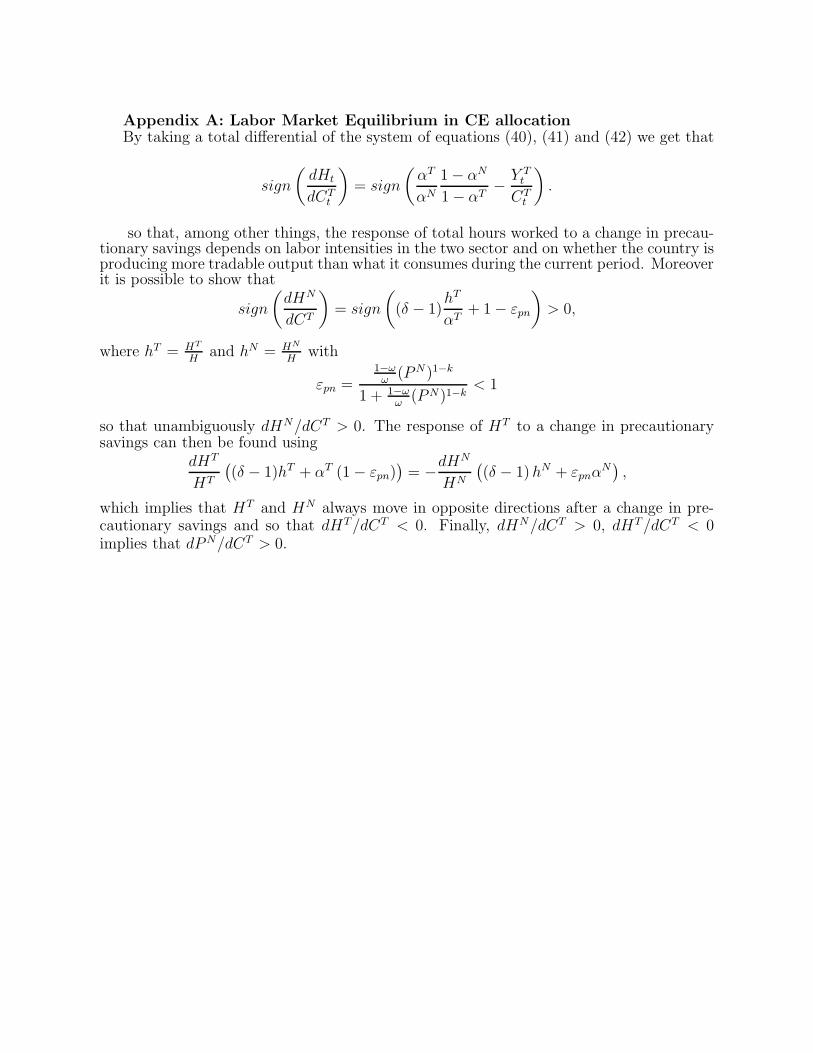
Appendix A: Labor Market Equilibrium in CE allocationBy taking a total differential of the system of equations (40), (41) and (42) we get that
sign
(dHt
dCTt
)= sign
(αT
αN
1− αN
1− αT− Y T
t
CTt
).
so that, among other things, the response of total hours worked to a change in precau-tionary savings depends on labor intensities in the two sector and on whether the country isproducing more tradable output than what it consumes during the current period. Moreoverit is possible to show that
sign
(dHN
dCT
)= sign
((δ − 1)
hT
αT+ 1− εpn
)> 0,
where hT = HT
Hand hN = HN
Hwith
εpn =1−ωω
(PN)1−k
1 + 1−ωω
(PN)1−k< 1
so that unambiguously dHN/dCT > 0. The response of HT to a change in precautionarysavings can then be found using
dHT
HT
((δ − 1)hT + αT (1− εpn)
)= −dHN
HN
((δ − 1)hN + εpnα
N),
which implies that HT and HN always move in opposite directions after a change in pre-cautionary savings and so that dHT/dCT < 0. Finally, dHN/dCT > 0, dHT/dCT < 0implies that dPN/dCT > 0.
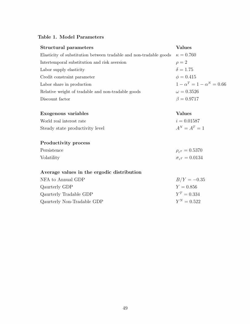
Table 1. Model Parameters
Structural parameters Values
Elasticity of substitution between tradable and non-tradable goods κ = 0.760
Intertemporal substitution and risk aversion ρ = 2
Labor supply elasticity δ = 1.75
Credit constraint parameter φ = 0.415
Labor share in production 1− αT = 1− αN = 0.66
Relative weight of tradable and non-tradable goods ω = 0.3526
Discount factor β = 0.9717
Exogenous variables Values
World real interest rate i = 0.01587
Steady state productivity level AN = AT = 1
Productivity process
Persistence ρεT = 0.5370
Volatility σεT = 0.0134
Average values in the ergodic distribution
NFA to Annual GDP B/Y = −0.35
Qaurterly GDP Y = 0.856
Qaurterly Tradable GDP Y T = 0.334
Qaurterly Non-Tradable GDP Y N = 0.522
49
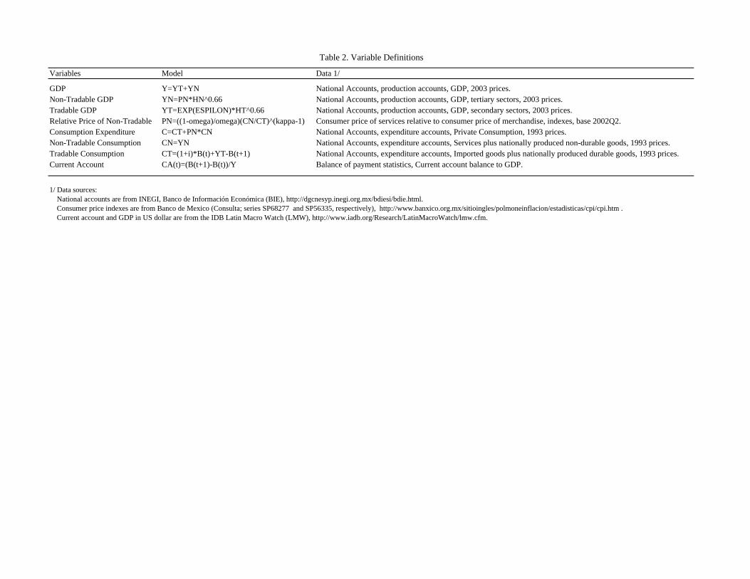
Table 2. Variable Definitions
Variables Model Data 1/
GDP Y=YT+YN National Accounts, production accounts, GDP, 2003 prices.Non-Tradable GDP YN=PN*HN^0.66 National Accounts, production accounts, GDP, tertiary sectors, 2003 prices.Tradable GDP YT=EXP(ESPILON)*HT^0.66 National Accounts, production accounts, GDP, secondary sectors, 2003 prices.Relative Price of Non-Tradable PN=((1-omega)/omega)(CN/CT)^(kappa-1) Consumer price of services relative to consumer price of merchandise, indexes, base 2002Q2. Consumption Expenditure C=CT+PN*CN National Accounts, expenditure accounts, Private Consumption, 1993 prices.Non-Tradable Consumption CN=YN National Accounts, expenditure accounts, Services plus nationally produced non-durable goods, 1993 prices.Tradable Consumption CT=(1+i)*B(t)+YT-B(t+1) National Accounts, expenditure accounts, Imported goods plus nationally produced durable goods, 1993 prices.Current Account CA(t)=(B(t+1)-B(t))/Y Balance of payment statistics, Current account balance to GDP.
1/ Data sources: National accounts are from INEGI, Banco de Información Económica (BIE), http://dgcnesyp.inegi.org.mx/bdiesi/bdie.html. Consumer price indexes are from Banco de Mexico (Consulta; series SP68277 and SP56335, respectively), http://www.banxico.org.mx/sitioingles/polmoneinflacion/estadisticas/cpi/cpi.htm . Current account and GDP in US dollar are from the IDB Latin Macro Watch (LMW), http://www.iadb.org/Research/LatinMacroWatch/lmw.cfm.
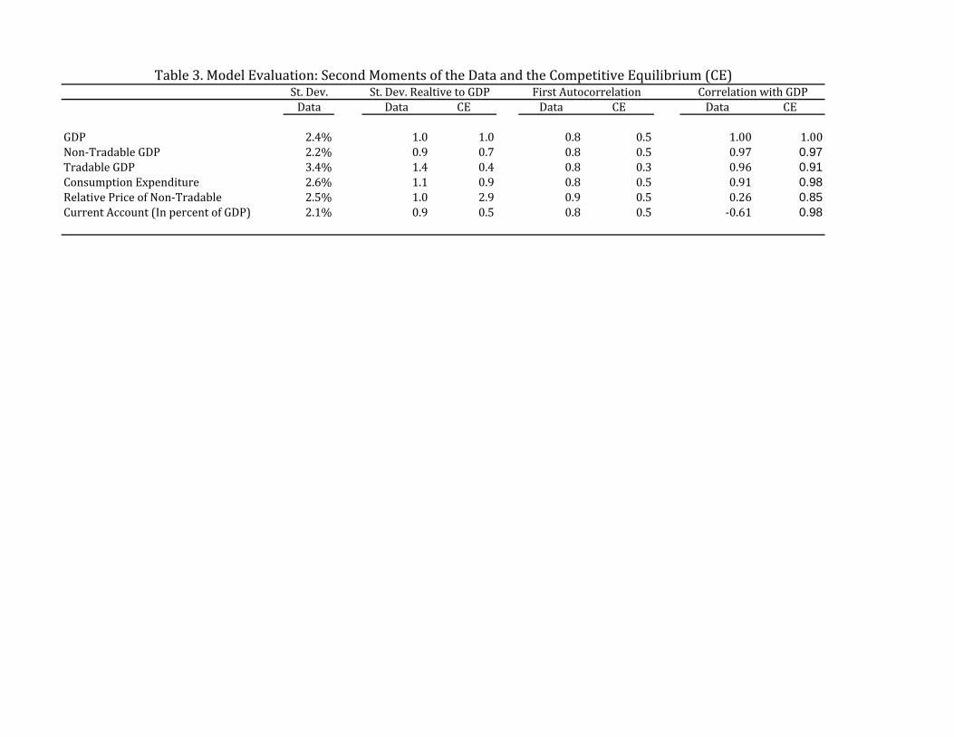
Table 3. Model Evaluation: Second Moments of the Data and the Competitive Equilibrium (CE)St. Dev. St. Dev. Realtive to GDP First Autocorrelation Correlation with GDPData Data CE Data CE Data CE
GDP 2.4% 1.0 1.0 0.8 0.5 1.00 1.00Non‐Tradable GDP 2.2% 0.9 0.7 0.8 0.5 0.97 0.97Tradable GDP 3.4% 1.4 0.4 0.8 0.3 0.96 0.91Consumption Expenditure 2.6% 1.1 0.9 0.8 0.5 0.91 0.98Relative Price of Non‐Tradable 2.5% 1.0 2.9 0.9 0.5 0.26 0.85Current Account (In percent of GDP) 2.1% 0.9 0.5 0.8 0.5 ‐0.61 0.98
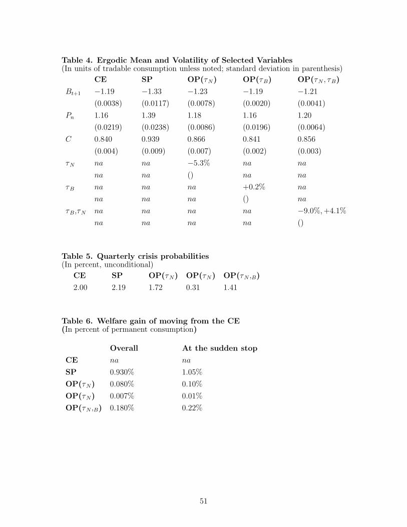
Table 4. Ergodic Mean and Volatility of Selected Variables(In units of tradable consumption unless noted; standard deviation in parenthesis)
CE SP OP(τN) OP(τB) OP(τN , τB)
Bt+1 −1.19 −1.33 −1.23 −1.19 −1.21
(0.0038) (0.0117) (0.0078) (0.0020) (0.0041)
Pn 1.16 1.39 1.18 1.16 1.20
(0.0219) (0.0238) (0.0086) (0.0196) (0.0064)
C 0.840 0.939 0.866 0.841 0.856
(0.004) (0.009) (0.007) (0.002) (0.003)
τN na na −5.3% na na
na na () na na
τB na na na +0.2% na
na na na () na
τB,τN na na na na −9.0%,+4.1%
na na na na ()
Table 5. Quarterly crisis probabilities(In percent, unconditional)
CE SP OP(τN) OP(τN) OP(τN ,B)
2.00 2.19 1.72 0.31 1.41
Table 6. Welfare gain of moving from the CE(In percent of permanent consumption)
Overall At the sudden stop
CE na na
SP 0.930% 1.05%
OP(τN) 0.080% 0.10%
OP(τN) 0.007% 0.01%
OP(τN ,B) 0.180% 0.22%
51
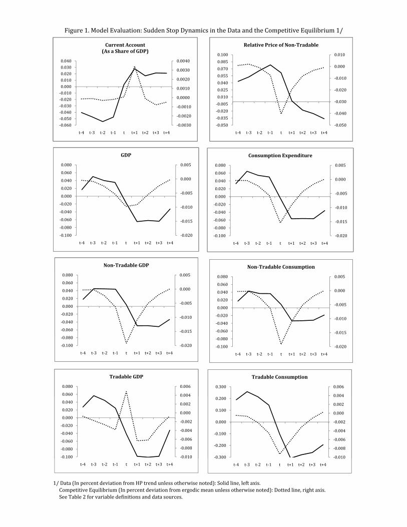
Figure 1. Model Evaluation: Sudden Stop Dynamics in the Data and the Competitive Equilibrium 1/
‐0.020
‐0.010
0.000
0.010
0.0250.0400.0550.0700.0850.100
Relative Price of NonTradable
0.0010
0.0020
0.0030
0.0040
0 0100.0000.0100.0200.0300.040
Current Account (As a Share of GDP)
‐0.050
‐0.040
‐0.030
‐0.020
‐0.010
0.000
0.010
‐0.050‐0.035‐0.020‐0.0050.0100.0250.0400.0550.0700.0850.100
t‐4 t‐3 t‐2 t‐1 t t+1 t+2 t+3 t+4
Relative Price of NonTradable
‐0.0030
‐0.0020
‐0.0010
0.0000
0.0010
0.0020
0.0030
0.0040
‐0.060‐0.050‐0.040‐0.030‐0.020‐0.0100.0000.0100.0200.0300.040
t‐4 t‐3 t‐2 t‐1 t t+1 t+2 t+3 t+4
Current Account (As a Share of GDP)
‐0.010
‐0.005
0.000
0.005
‐0.020
0.000
0.020
0.040
0.060
0.080
GDP
‐0.010
‐0.005
0.000
0.005
‐0.020
0.000
0.020
0.040
0.060
0.080
Consumption Expenditure
‐0.050
‐0.040
‐0.030
‐0.020
‐0.010
0.000
0.010
‐0.050‐0.035‐0.020‐0.0050.0100.0250.0400.0550.0700.0850.100
t‐4 t‐3 t‐2 t‐1 t t+1 t+2 t+3 t+4
Relative Price of NonTradable
‐0.0030
‐0.0020
‐0.0010
0.0000
0.0010
0.0020
0.0030
0.0040
‐0.060‐0.050‐0.040‐0.030‐0.020‐0.0100.0000.0100.0200.0300.040
t‐4 t‐3 t‐2 t‐1 t t+1 t+2 t+3 t+4
Current Account (As a Share of GDP)
‐0.020
‐0.015
‐0.010
‐0.005
0.000
0.005
‐0.100
‐0.080
‐0.060
‐0.040
‐0.020
0.000
0.020
0.040
0.060
0.080
t‐4 t‐3 t‐2 t‐1 t t+1 t+2 t+3 t+4
GDP
‐0.020
‐0.015
‐0.010
‐0.005
0.000
0.005
‐0.100
‐0.080
‐0.060
‐0.040
‐0.020
0.000
0.020
0.040
0.060
0.080
t‐4 t‐3 t‐2 t‐1 t t+1 t+2 t+3 t+4
Consumption Expenditure
NonTradable GDP NonTradable Consumption
‐0.050
‐0.040
‐0.030
‐0.020
‐0.010
0.000
0.010
‐0.050‐0.035‐0.020‐0.0050.0100.0250.0400.0550.0700.0850.100
t‐4 t‐3 t‐2 t‐1 t t+1 t+2 t+3 t+4
Relative Price of NonTradable
‐0.0030
‐0.0020
‐0.0010
0.0000
0.0010
0.0020
0.0030
0.0040
‐0.060‐0.050‐0.040‐0.030‐0.020‐0.0100.0000.0100.0200.0300.040
t‐4 t‐3 t‐2 t‐1 t t+1 t+2 t+3 t+4
Current Account (As a Share of GDP)
‐0.020
‐0.015
‐0.010
‐0.005
0.000
0.005
‐0.100
‐0.080
‐0.060
‐0.040
‐0.020
0.000
0.020
0.040
0.060
0.080
t‐4 t‐3 t‐2 t‐1 t t+1 t+2 t+3 t+4
GDP
‐0.020
‐0.015
‐0.010
‐0.005
0.000
0.005
‐0.100
‐0.080
‐0.060
‐0.040
‐0.020
0.000
0.020
0.040
0.060
0.080
t‐4 t‐3 t‐2 t‐1 t t+1 t+2 t+3 t+4
Consumption Expenditure
‐0.015
‐0.010
‐0.005
0.000
0.005
‐0.060
‐0.040
‐0.020
0.000
0.020
0.040
0.060
0.080
NonTradable GDP
‐0.015
‐0.010
‐0.005
0.000
0.005
‐0.060
‐0.040
‐0.020
0.000
0.020
0.040
0.060
0.080
NonTradable Consumption
‐0.050
‐0.040
‐0.030
‐0.020
‐0.010
0.000
0.010
‐0.050‐0.035‐0.020‐0.0050.0100.0250.0400.0550.0700.0850.100
t‐4 t‐3 t‐2 t‐1 t t+1 t+2 t+3 t+4
Relative Price of NonTradable
‐0.0030
‐0.0020
‐0.0010
0.0000
0.0010
0.0020
0.0030
0.0040
‐0.060‐0.050‐0.040‐0.030‐0.020‐0.0100.0000.0100.0200.0300.040
t‐4 t‐3 t‐2 t‐1 t t+1 t+2 t+3 t+4
Current Account (As a Share of GDP)
‐0.020
‐0.015
‐0.010
‐0.005
0.000
0.005
‐0.100
‐0.080
‐0.060
‐0.040
‐0.020
0.000
0.020
0.040
0.060
0.080
t‐4 t‐3 t‐2 t‐1 t t+1 t+2 t+3 t+4
GDP
‐0.020
‐0.015
‐0.010
‐0.005
0.000
0.005
‐0.100
‐0.080
‐0.060
‐0.040
‐0.020
0.000
0.020
0.040
0.060
0.080
t‐4 t‐3 t‐2 t‐1 t t+1 t+2 t+3 t+4
Consumption Expenditure
‐0.020
‐0.015
‐0.010
‐0.005
0.000
0.005
‐0.100
‐0.080
‐0.060
‐0.040
‐0.020
0.000
0.020
0.040
0.060
0.080
t‐4 t‐3 t‐2 t‐1 t t+1 t+2 t+3 t+4
NonTradable GDP
0.004
0.006
0.060
0.080
Tradable GDP
‐0.020
‐0.015
‐0.010
‐0.005
0.000
0.005
‐0.100
‐0.080
‐0.060
‐0.040
‐0.020
0.000
0.020
0.040
0.060
0.080
t‐4 t‐3 t‐2 t‐1 t t+1 t+2 t+3 t+4
NonTradable Consumption
0 004
0.0060.300
Tradable Consumption
‐0.050
‐0.040
‐0.030
‐0.020
‐0.010
0.000
0.010
‐0.050‐0.035‐0.020‐0.0050.0100.0250.0400.0550.0700.0850.100
t‐4 t‐3 t‐2 t‐1 t t+1 t+2 t+3 t+4
Relative Price of NonTradable
‐0.0030
‐0.0020
‐0.0010
0.0000
0.0010
0.0020
0.0030
0.0040
‐0.060‐0.050‐0.040‐0.030‐0.020‐0.0100.0000.0100.0200.0300.040
t‐4 t‐3 t‐2 t‐1 t t+1 t+2 t+3 t+4
Current Account (As a Share of GDP)
‐0.020
‐0.015
‐0.010
‐0.005
0.000
0.005
‐0.100
‐0.080
‐0.060
‐0.040
‐0.020
0.000
0.020
0.040
0.060
0.080
t‐4 t‐3 t‐2 t‐1 t t+1 t+2 t+3 t+4
GDP
‐0.020
‐0.015
‐0.010
‐0.005
0.000
0.005
‐0.100
‐0.080
‐0.060
‐0.040
‐0.020
0.000
0.020
0.040
0.060
0.080
t‐4 t‐3 t‐2 t‐1 t t+1 t+2 t+3 t+4
Consumption Expenditure
‐0.020
‐0.015
‐0.010
‐0.005
0.000
0.005
‐0.100
‐0.080
‐0.060
‐0.040
‐0.020
0.000
0.020
0.040
0.060
0.080
t‐4 t‐3 t‐2 t‐1 t t+1 t+2 t+3 t+4
NonTradable GDP
‐0.010
‐0.008
‐0.006
‐0.004
‐0.002
0.000
0.002
0.004
0.006
‐0.100
‐0.080
‐0.060
‐0.040
‐0.020
0.000
0.020
0.040
0.060
0.080
Tradable GDP
‐0.020
‐0.015
‐0.010
‐0.005
0.000
0.005
‐0.100
‐0.080
‐0.060
‐0.040
‐0.020
0.000
0.020
0.040
0.060
0.080
t‐4 t‐3 t‐2 t‐1 t t+1 t+2 t+3 t+4
NonTradable Consumption
‐0.010
‐0.008
‐0.006
‐0.004
‐0.002
0.000
0.002
0.004
0.006
‐0.300
‐0.200
‐0.100
0.000
0.100
0.200
0.300
Tradable Consumption
1/ Data (In percent deviation from HP trend unless otherwise noted): Solid line, left axis. Competitive Equilibrium (In percent deviation from ergodic mean unless otherwise noted): Dotted line, right axis. See Table 2 for variable definitions and data sources.
‐0.050
‐0.040
‐0.030
‐0.020
‐0.010
0.000
0.010
‐0.050‐0.035‐0.020‐0.0050.0100.0250.0400.0550.0700.0850.100
t‐4 t‐3 t‐2 t‐1 t t+1 t+2 t+3 t+4
Relative Price of NonTradable
‐0.0030
‐0.0020
‐0.0010
0.0000
0.0010
0.0020
0.0030
0.0040
‐0.060‐0.050‐0.040‐0.030‐0.020‐0.0100.0000.0100.0200.0300.040
t‐4 t‐3 t‐2 t‐1 t t+1 t+2 t+3 t+4
Current Account (As a Share of GDP)
‐0.020
‐0.015
‐0.010
‐0.005
0.000
0.005
‐0.100
‐0.080
‐0.060
‐0.040
‐0.020
0.000
0.020
0.040
0.060
0.080
t‐4 t‐3 t‐2 t‐1 t t+1 t+2 t+3 t+4
GDP
‐0.020
‐0.015
‐0.010
‐0.005
0.000
0.005
‐0.100
‐0.080
‐0.060
‐0.040
‐0.020
0.000
0.020
0.040
0.060
0.080
t‐4 t‐3 t‐2 t‐1 t t+1 t+2 t+3 t+4
Consumption Expenditure
‐0.020
‐0.015
‐0.010
‐0.005
0.000
0.005
‐0.100
‐0.080
‐0.060
‐0.040
‐0.020
0.000
0.020
0.040
0.060
0.080
t‐4 t‐3 t‐2 t‐1 t t+1 t+2 t+3 t+4
NonTradable GDP
‐0.010
‐0.008
‐0.006
‐0.004
‐0.002
0.000
0.002
0.004
0.006
‐0.100
‐0.080
‐0.060
‐0.040
‐0.020
0.000
0.020
0.040
0.060
0.080
t‐4 t‐3 t‐2 t‐1 t t+1 t+2 t+3 t+4
Tradable GDP
‐0.020
‐0.015
‐0.010
‐0.005
0.000
0.005
‐0.100
‐0.080
‐0.060
‐0.040
‐0.020
0.000
0.020
0.040
0.060
0.080
t‐4 t‐3 t‐2 t‐1 t t+1 t+2 t+3 t+4
NonTradable Consumption
‐0.010
‐0.008
‐0.006
‐0.004
‐0.002
0.000
0.002
0.004
0.006
‐0.300
‐0.200
‐0.100
0.000
0.100
0.200
0.300
t‐4 t‐3 t‐2 t‐1 t t+1 t+2 t+3 t+4
Tradable Consumption
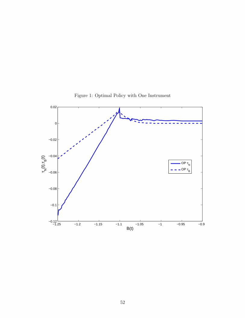
Figure 1: Optimal Policy with One Instrument
−1.25 −1.2 −1.15 −1.1 −1.05 −1 −0.95 −0.9−0.12
−0.1
−0.08
−0.06
−0.04
−0.02
0
0.02
B(t)
τ N(t
),τ B
(t)
OP τN
OP τB
52
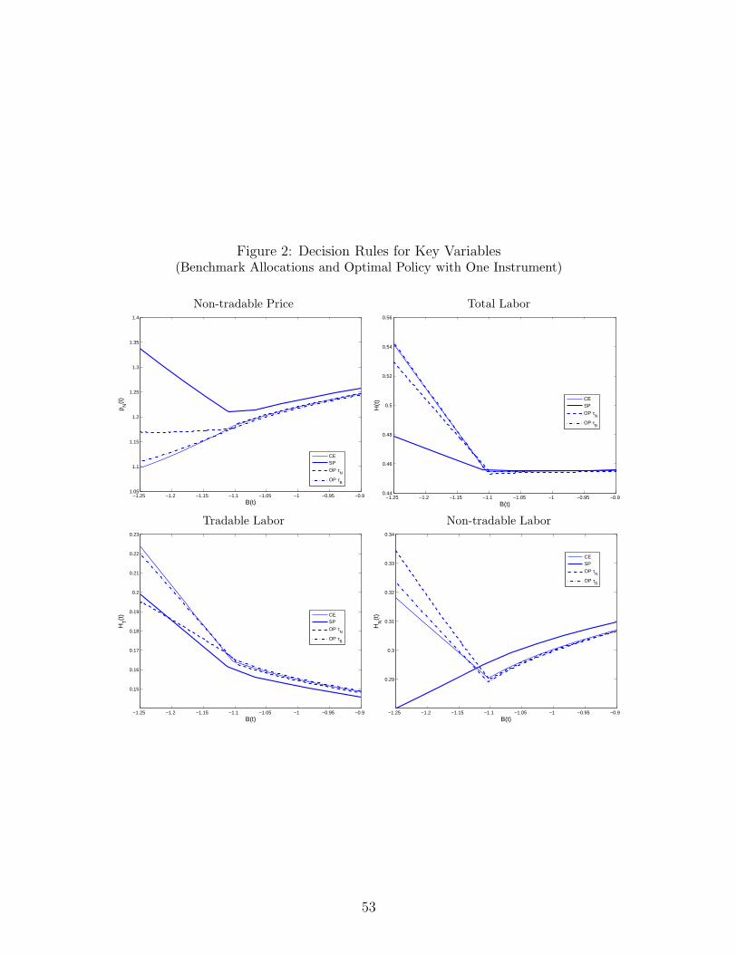
Figure 2: Decision Rules for Key Variables(Benchmark Allocations and Optimal Policy with One Instrument)
Non-tradable Price
−1.25 −1.2 −1.15 −1.1 −1.05 −1 −0.95 −0.91.05
1.1
1.15
1.2
1.25
1.3
1.35
1.4
B(t)
p N(t
)
CESP
OP τN
OP τB
Total Labor
−1.25 −1.2 −1.15 −1.1 −1.05 −1 −0.95 −0.90.44
0.46
0.48
0.5
0.52
0.54
0.56
B(t)
H(t
)
CESP
OP τN
OP τB
Tradable Labor
−1.25 −1.2 −1.15 −1.1 −1.05 −1 −0.95 −0.9
0.15
0.16
0.17
0.18
0.19
0.2
0.21
0.22
0.23
B(t)
HT(t
)
CESP
OP τN
OP τB
Non-tradable Labor
−1.25 −1.2 −1.15 −1.1 −1.05 −1 −0.95 −0.9
0.29
0.3
0.31
0.32
0.33
0.34
B(t)
HN(t
)
CESP
OP τN
OP τB
53
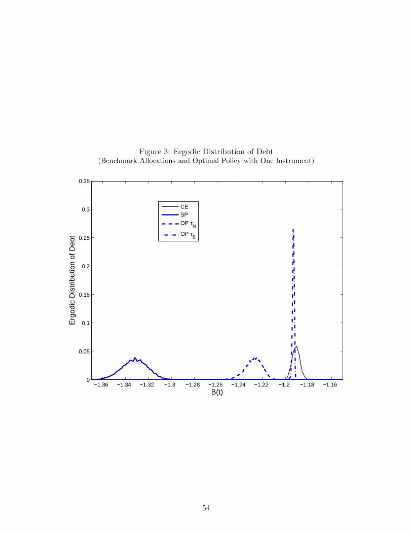
Figure 3: Ergodic Distribution of Debt(Benchmark Allocations and Optimal Policy with One Instrument)
−1.36 −1.34 −1.32 −1.3 −1.28 −1.26 −1.24 −1.22 −1.2 −1.18 −1.160
0.05
0.1
0.15
0.2
0.25
0.3
0.35
B(t)
Erg
odic
Dis
trib
utio
n of
Deb
t
CESP
OP τN
OP τB
54
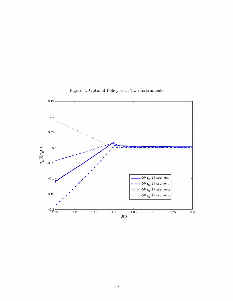
Figure 4: Optimal Policy with Two Instruments
−1.25 −1.2 −1.15 −1.1 −1.05 −1 −0.95 −0.9−0.2
−0.15
−0.1
−0.05
0
0.05
0.1
0.15
B(t)
τ N(t
),τ B
(t)
OP τN
, 1 instrument
OP τB, 1 instrument
OP τN
, 2 instruments
OP τB, 2 instruments
55
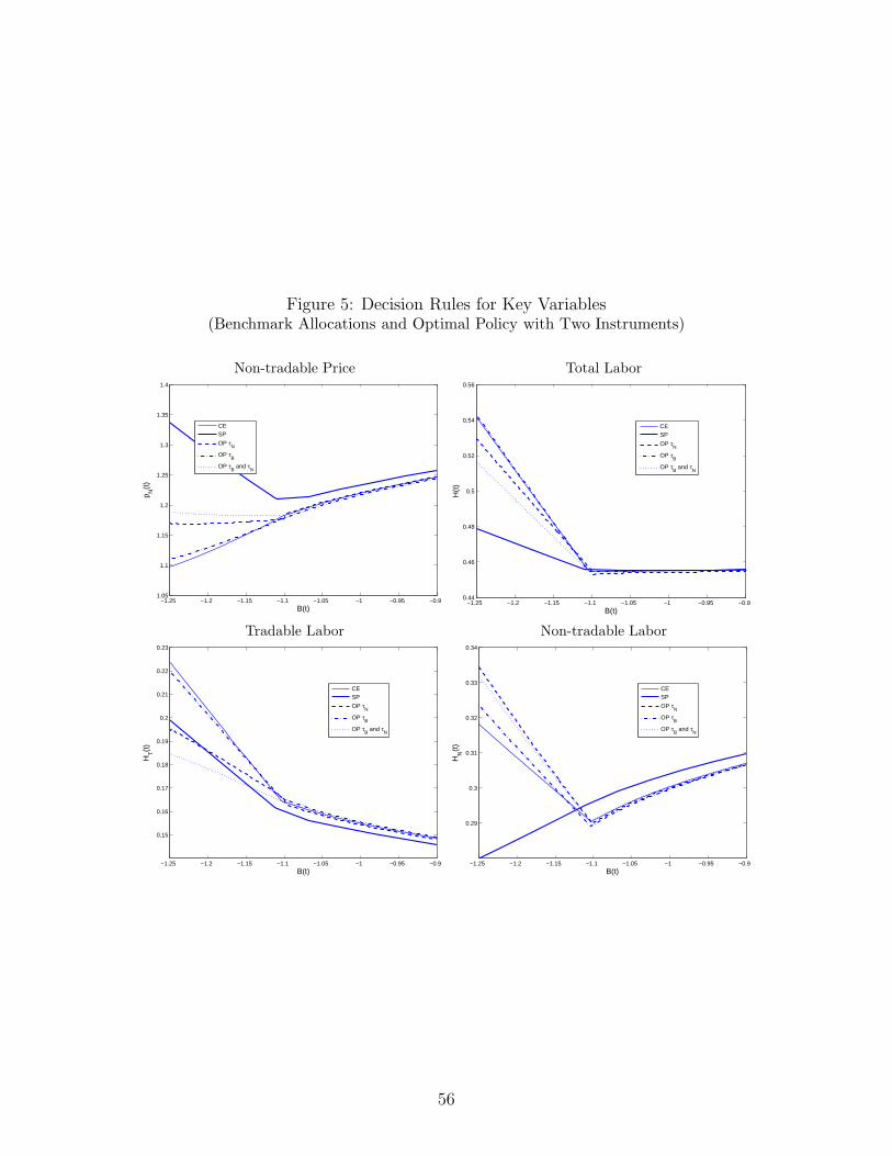
Figure 5: Decision Rules for Key Variables(Benchmark Allocations and Optimal Policy with Two Instruments)
Non-tradable Price
−1.25 −1.2 −1.15 −1.1 −1.05 −1 −0.95 −0.91.05
1.1
1.15
1.2
1.25
1.3
1.35
1.4
B(t)
p N(t
)
CESP
OP τN
OP τB
OP τB and τ
N
Total Labor
−1.25 −1.2 −1.15 −1.1 −1.05 −1 −0.95 −0.90.44
0.46
0.48
0.5
0.52
0.54
0.56
B(t)
H(t
)
CESP
OP τN
OP τB
OP τB and τ
N
Tradable Labor
−1.25 −1.2 −1.15 −1.1 −1.05 −1 −0.95 −0.9
0.15
0.16
0.17
0.18
0.19
0.2
0.21
0.22
0.23
B(t)
HT(t
)
CESP
OP τN
OP τB
OP τB and τ
N
Non-tradable Labor
−1.25 −1.2 −1.15 −1.1 −1.05 −1 −0.95 −0.9
0.29
0.3
0.31
0.32
0.33
0.34
B(t)
HN(t
)
CESP
OP τN
OP τB
OP τB and τ
N
56
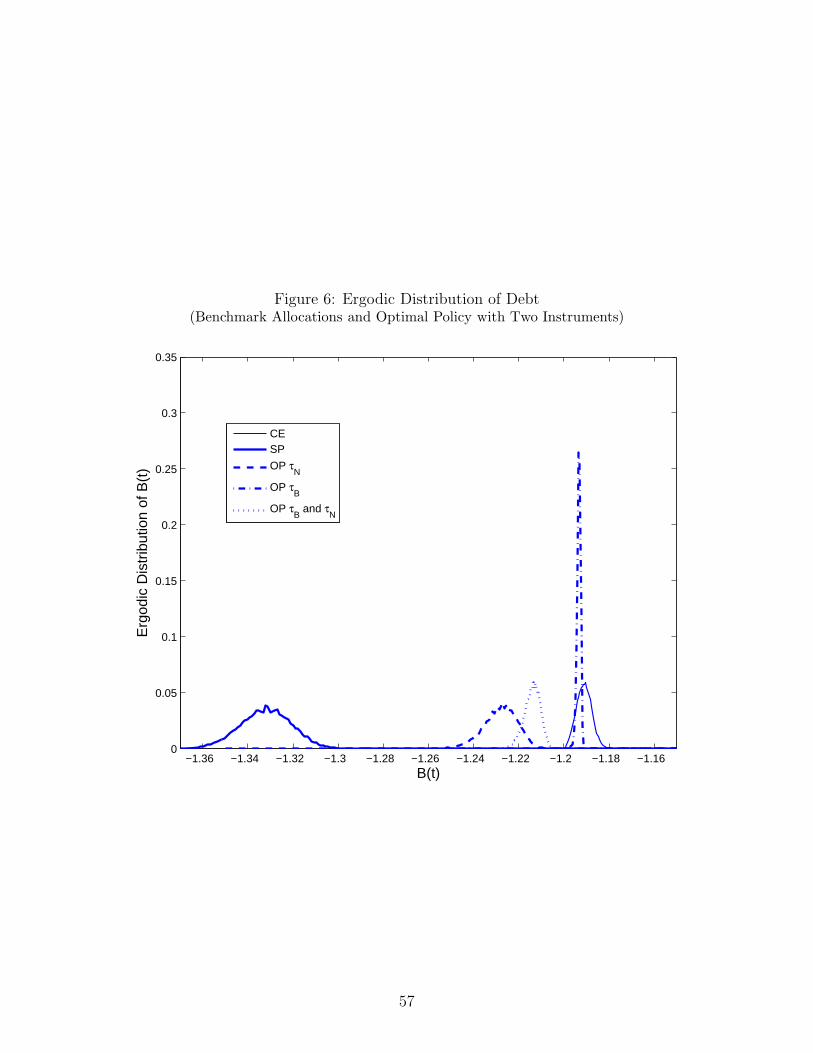
Figure 6: Ergodic Distribution of Debt(Benchmark Allocations and Optimal Policy with Two Instruments)
−1.36 −1.34 −1.32 −1.3 −1.28 −1.26 −1.24 −1.22 −1.2 −1.18 −1.160
0.05
0.1
0.15
0.2
0.25
0.3
0.35
B(t)
Erg
odic
Dis
trib
utio
n of
B(t
)
CESP
OP τN
OP τB
OP τB and τ
N
57