Optimal Maintenance of a Production System with L

Hindawi Publishing CorporationMathematical Problems in EngineeringVolume 2012, Article ID 673864, 14 pagesdoi:10.1155/2012/673864

Research ArticleOptimal Maintenance of a Production System withL Intermediate Buffers

Constantinos C. Karamatsoukis1

and Epaminondas G. Kyriakidis2

1 Department of Financial and Management Engineering, University of the Aegean,Kountouriotou 41, 82100 Chios, Greece

2 Department of Statistics, Athens University of Business and Economics, 76 Patission Street,10434 Athens, Greece

Correspondence should be addressed to Epaminondas G. Kyriakidis, [email protected]

Received 29 May 2012; Accepted 23 July 2012

Academic Editor: Carlo Cattani

Copyright q 2012 C. C. Karamatsoukis and E. G. Kyriakidis. This is an open access articledistributed under the Creative Commons Attribution License, which permits unrestricted use,distribution, and reproduction in any medium, provided the original work is properly cited.

We consider a production-inventory system that consists of an input-generating installation, aproduction unit and L intermediate buffers. It is assumed that the installation transfers the rawmaterial j ∈ {1, . . . , L} to buffer Bj, and the production unit pulls the rawmaterial j ∈ {1, ..., L} frombuffer Bj. We consider the problem of the optimal preventive maintenance of the installation if theinstallation deteriorates stochastically with usage and the production unit is always in operativecondition. We also consider the problem of the optimal preventive maintenance of the productionunit if the production unit deteriorates stochastically with usage and the installation is alwaysin operative condition. Under a suitable cost structure and for given contents of the buffers, it isproved that the average-cost optimal policy for the first (second) problem initiates a preventivemaintenance of the installation (production unit) if and only if the degree of deterioration of theinstallation (production unit) exceeds some critical level. Numerical results are presented for bothproblems.

1. Introduction

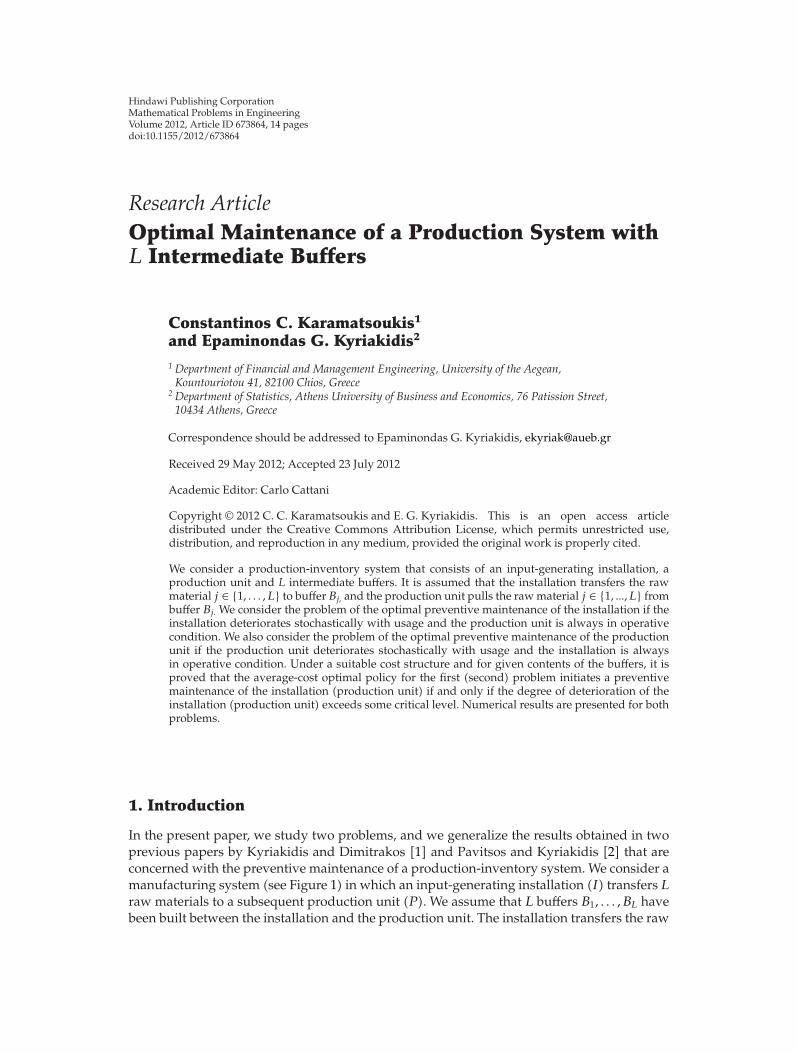
In the present paper, we study two problems, and we generalize the results obtained in twoprevious papers by Kyriakidis and Dimitrakos [1] and Pavitsos and Kyriakidis [2] that areconcerned with the preventive maintenance of a production-inventory system. We consider amanufacturing system (see Figure 1) in which an input-generating installation (I) transfers Lraw materials to a subsequent production unit (P). We assume that L buffers B1, . . . , BL havebeen built between the installation and the production unit. The installation transfers the raw

2 Mathematical Problems in Engineering

B1

B2

BL

IP

p1

p2

pL dL

d2

d1

...

Figure 1: The production-inventory system.

material j ∈ {1, . . . , L} to the buffer Bj , and the production unit pulls this raw material fromthe buffer Bj . The buffers have finite capacities.

In the first problem it is assumed that the installation deteriorates stochastically overtime, and the production unit is always in operative condition. The deteriorating processfor the installation is described by some known transition probabilities between differentdegrees of deterioration. A discrete-time Markov decision model is considered for theoptimal preventive maintenance of the installation. The maintenance times are assumed to begeometrically distributed, and the cost structure includes operating costs of the installation,costs for storing the raw materials in the buffers, maintenance costs and costs due toproduction delay when the installation does not operate or operate partially and the contentsof some or all buffers are below some specific levels. It is proved that for fixed contents ofthe buffers the policy that minimizes the long-run expected average cost per unit time isof control-limit type, that is, it initiates a preventive maintenance of the installation if andonly if its degree of deterioration exceeds some critical level. This result generalizes thestructural result that was obtained by Kyriakidis and Dimitrakos [1] for the case in whichL = 1. In the second problem it is assumed that the production unit deteriorates stochasticallyover time and the installation is always in operative condition. The deteriorating process forthe production unit is described by some known transition probabilities between differentdegrees of deterioration. A discrete-time Markov decision model is formulated for theoptimal preventive maintenance of the production unit. The maintenance times are assumedto be geometrically distributed, and the cost structure includes operating costs of theproduction unit, costs for the maintenance of the production unit, storage costs, penalty costs,and costs due to the lost production. It is proved that for fixed contents of the buffers theaverage-cost optimal policy is again of control-limit type, that is, it initiates a preventivemaintenance of the production unit if and only if its degree of deterioration exceeds somecritical level. This result generalizes the structural result that was obtained by Pavitsos andKyriakidis [2] for the case in which L = 1.

An example of this system could be a production machine that pulls L different partsfrom L buffers and assembles them in order to produce the final product. These parts aretransferred by a feeder to the buffers. Note that in the last twenty years a great numberof maintenance models for production-inventory systems have been studied (see Van DerDuyn Schouten and Vanneste [3], Meller and Kim [4], Iravani and Duenyas [5], Sloan [6],Yao et al. [7], Rezg et al. [8], Dimitrakos and Kyriakidis [9], Karamatsoukis and Kyriakidis[10], and Hadidi et al. [11]). In these models, the preventive maintenance depends on theworking condition of a machine and the level of a subsequent buffer. The first problem

Mathematical Problems in Engineering 3

that we study in the present paper has its origin in a model introduced by Van Der DuynSchouten and Vanneste [3]. The states of that model consist of the age of a machine and thecontent of a subsequent buffer that is fed by the machine. The cost structure included costsdue to lost production that were incurred when a repair was performed on the machine andthe buffer was empty. The repair times of the machine were assumed to be geometricallydistributed. It was proved that, for fixed buffer content, the average-cost optimal policyinitiates a preventive maintenance of the machine if and only if its age is greater than orequal to a critical value.

The rest of the paper is organized as follows. In the next section, we describe theproblem in which only the installation deteriorates with usage, and we derive the structure ofthe average-cost optimal policy. In Section 3, we study the case in which only the productionunit deteriorates over time, and the structure of the average-cost optimal policy is derived.Numerical results are presented for both problems. In the final section, the main conclusionsof the paper are summarized, and we propose topics for future research.

2. The Problem when the Installation Deteriorates Stochastically

We consider a production-inventory system (see Figure 1) which consists of an installation(I) that supplies the buffer Bj with the raw material j ∈ {1, . . . , L} and a production unit(P) which pulls dj units of the raw material j ∈ {1, . . . , L} from buffer Bj during one unitof time. It is assumed that the production unit is always in operative condition, and that theinstallation may fail as time evolves. The buffer Bj, j = 1, 2, . . . , L has finite capacity which isequal to Kj units of raw material j. As long as the buffer Bj, j = 1, . . . , L is not full and theinstallation is in operative condition, the installation may transfer pj(> dj) units of the rawmaterial j ∈ {1, . . . , L} to buffer Bj during one unit of time and the difference pj − dj is storedin buffer Bj . As soon as buffer Bj, j = 1, . . . , L is filled up the installation reduces its speedfrom pj to dj . The numbers pj , dj ,Kj , j = 1, . . . , L are assumed to be integers.

We suppose that the installation is inspected at discrete, equidistant time epochsτ = 0, 1, . . . (say every day), and is classified into one of m + 2 working conditions0, 1, . . . , m + 1 which describe increasing levels of deterioration. Working condition 0 denotesa new installation (or functioning as good as new), while working conditionm+1 means thatthe installation is in failed (inoperative) condition and it cannot transfer the raw materialsto the buffers. The intermediate working conditions 1, . . . , m are operative and are orderedascendingly to reflect their relative degree of deterioration. The transition probability ofmoving from working condition i at time epoch τ to working condition r at time epochτ + 1 is equal to pir . We assume that the probability of eventually reaching the workingcondition m + 1 from any initial working condition i is nonzero. If at a time epoch τ theinstallation is found to be at failure state m + 1, a corrective maintenance is mandatory. If ata time epoch τ the installation is found to be at any working condition i ≤ m, a preventivemaintenance may be initiated. When a preventive maintenance is performed, the installationdoes not operate and it does not transfer any raw material to its buffer. It is assumed that thepreventive and corrective repair times (expressed in time units) are geometrically distributedwith probability of success aI and bI , that is, the probability that they will last t ≥ 1 time unitsare equal to (1 − aI)

t−1aI and (1 − bI)t−1bI , respectively. When a preventive or a corrective

maintenance is performed and the buffer Bj, j ∈ {1, . . . , L} contains xj units of raw materialj, the production unit pulls from buffer Bj during one unit of time min(xj , dj) units of rawmaterial j. Both maintenances bring the installation to its perfect condition 0.


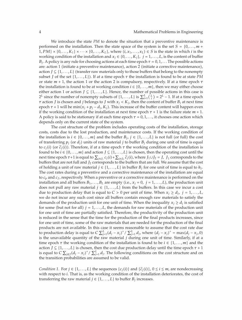
We introduce the state PM to denote the situation that a preventive maintenance isperformed on the installation. Then the state space of the system is the set S = {0, . . . , m +1, PM} × {0, . . . , K1} × · · · × {0, . . . , KL}, where (i, x1, . . . , xL) ∈ S is the state in which i is theworking condition of the installation and xj ∈ {0, . . . , Kj}, j = 1, . . . , L, is the content of bufferBj . A policy is any rule for choosing actions at each time epoch τ = 0, 1, . . . The possible actionsare: action 1 (initiate a preventive maintenance), action 2 (initiate a corrective maintenance),action J ⊆ {1, . . . , L} (transfer rawmaterials only to those buffers that belong to the nonemptysubset J of the set {1, . . . , L}). If at a time epoch τ the installation is found to be at state PMor state m + 1, the action 1 or the action 2 is compulsory, respectively. If at a time epoch τthe installation is found to be at working condition i ∈ {0, . . . , m}, then we may either chooseeither action 1 or action J ⊆ {1, . . . , L}. Hence, the number of possible actions in this case is2L since the number of nonempty subsets of {1, . . . , L} is ∑L

i=1(Li

)= 2L − 1. If at a time epoch

τ action J is chosen and j belongs to J with xj < Kj , then the content of buffer Bj at next timeepoch τ + 1 will be min(xj + pj − dj,Kj). This increase of the buffer content will happen evenif the working condition of the installation at next time epoch τ + 1 is the failure state m + 1.A policy is said to be stationary if at each time epoch τ = 0, 1, . . ., it chooses one action whichdepends only on the current state of the system.

The cost structure of the problem includes operating costs of the installation, storagecosts, costs due to the lost production, and maintenance costs. If the working condition ofthe installation is i ∈ {0, . . . , m} and the buffer Bj, j ∈ {1, . . . , L} is not full (or full) the costof transferring pj (or dj) units of raw material j to buffer Bj during one unit of time is equalto cj(i) (or c̃j(i)). Therefore, if at a time epoch τ the working condition of the installation isfound to be i ∈ {0, . . . , m} and action J ⊆ {1, . . . , L} is chosen, then the operating cost until thenext time epoch τ+1 is equal to

∑j∈J1 cj(i)+

∑j∈J2 c̃j(i),where J1∪J2 = J, J1 corresponds to the

buffers that are not full and J2 corresponds to the buffers that are full. We assume that the costof holding a unit of raw material j ∈ {1, . . . , L} in buffer Bj for one unit of time is equal to hj .The cost rates during a preventive and a corrective maintenance of the installation are equalto cp and cf , respectively. When a preventive or a corrective maintenance is performed on theinstallation and all buffers B1, . . . , BL are empty (i.e., xj = 0, j = 1, . . . , L), the production unitdoes not pull any raw material j ∈ {1, . . . , L} from the buffers. In this case we incur a costdue to production delay that is equal to C > 0 per unit of time. When xj ≥ dj , j = 1, . . . , L,we do not incur any such cost since all buffers contain enough raw materials to satisfy thedemands of the production unit for one unit of time. When the inequality xj ≥ dj is satisfiedfor some (but not for all) j = 1, . . . , L, the demands for raw materials of the production unitfor one unit of time are partially satisfied. Therefore, the productivity of the production unitis reduced in the sense that the time for the production of the final products increases, sincefor one unit of time, some of the raw materials that are needed for the production of the finalproducts are not available. In this case it seems reasonable to assume that the cost rate dueto production delay is equal to C

∑Lj=1(dj − xj)

+/∑L

j=1 dj, where (dj − xj)+ = max(dj − xj , 0)

is the unavailable quantity of the raw material j during one unit of time. Similarly, if at atime epoch τ the working condition of the installation is found to be i ∈ {1, . . . , m} and theaction J ⊆ {1, . . . , L} is chosen, then the cost due production delay until the time epoch τ + 1is equal to C

∑j/∈J(dj − xj)

+/∑L

j=1 dj. The following conditions on the cost structure and onthe transition probabilities are assumed to be valid.

Condition 1. For j ∈ {1, . . . , L} the sequences {cj(i)} and {c̃j(i)}, 0 ≤ i ≤ m, are nondecreasingwith respect to i. That is, as the working condition of the installation deteriorates, the cost oftransferring the raw material j ∈ {1, . . . , L} to buffer Bj increases.


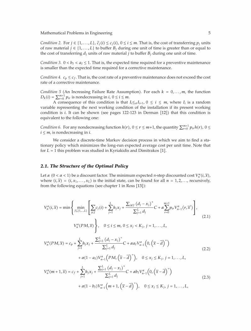
Condition 2. For j ∈ {1, . . . , L}, c̃j(i) ≤ cj(i), 0 ≤ i ≤ m. That is, the cost of transferring pj unitsof raw material j ∈ {1, . . . , L} to buffer Bj during one unit of time is greater than or equal tothe cost of transferring dj units of raw material j to buffer Bj during one unit of time.

Condition 3. 0 < bI < aI ≤ 1. That is, the expected time required for a preventive maintenanceis smaller than the expected time required for a corrective maintenance.

Condition 4. cp ≤ cf . That is, the cost rate of a preventive maintenance does not exceed the costrate of a corrective maintenance.

Condition 5 (An Increasing Failure Rate Assumption). For each k = 0, . . . , m, the functionDk(i) =

∑m+1r=k pir is nondecreasing in i, 0 ≤ i ≤ m.

A consequence of this condition is that Ii≤stIi+1, 0 ≤ i ≤ m, where Ii is a randomvariable representing the next working condition of the installation if its present workingcondition is i. It can be shown (see pages 122-123 in Derman [12]) that this condition isequivalent to the following one:

Condition 6. For any nondecreasing function h(r), 0 ≤ r ≤ m+1, the quantity∑m+1

r=0 pirh(r), 0 ≤i ≤ m, is nondecreasing in i.

We consider a discrete-time Markov decision process in which we aim to find a sta-tionary policy which minimizes the long-run expected average cost per unit time. Note thatfor L = 1 this problem was studied in Kyriakidis and Dimitrakos [1].

2.1. The Structure of the Optimal Policy

Let α (0 < α < 1) be a discount factor. The minimum expected n-step discounted cost V αn (i, x),

where (i, x) = (i, x1, . . . , xL) is the initial state, can be found for all n = 1, 2, . . ., recursively,from the following equations (see chapter 1 in Ross [13]):

V αn (i, x) = min

⎧⎨

⎩min

J⊆{1,...,L}

⎡

⎣∑

j∈Jcj(i) +

L∑

j=1

hjxj +

∑j/∈J

(dj − xj

)+

∑Lj=1 dj

C + αm+1∑

r=0

pirVαn−1

(r, x′)

⎤

⎦,

V αn (PM,x)

⎫⎬

⎭, 0 ≤ i ≤ m, 0 ≤ xj < Kj, j = 1, . . . , L,

(2.1)

V αn (PM,x) = cp +

L∑

j=1

hjxj +

∑Lj=1

(dj − xj

)+

∑Lj=1 dj

C + αaIVαn−1

(0,(x − d

)+)

+ α(1 − aI)V αn−1

(PM,

(x − d

)+), 0 ≤ xj ≤ Kj, j = 1, . . . , L,

(2.2)

V αn (m + 1, x) = cf +

L∑

j=1

hjxj +

∑Lj=1

(dj − xj

)+

∑Lj=1 dj

C + αbIVαn−1

(0,(x − d

)+)

+ α(1 − bI)V αn−1

(m + 1,

(x − d

)+), 0 ≤ xj ≤ Kj, j = 1, . . . , L,

(2.3)


where x′ in (2.1) is a vector with L components in which the jth component equals to min(xj+pj −dj,Kj), if j ∈ J , while, if j /∈ J , it is equal to (xj −dj)

+ = max(xj −dj, 0) and (x−d)+ in (2.2),and (2.3) is the vector ((x1−d1)

+, . . . , (xL−dL)+). The initial condition is V α

0 (s) = 0, s ∈ S. Notethat, if xj = Kj for some values of j ∈ {1, . . . , L}, (2.1) is valid if cj(i) is changed to c̃j(i) forthese values of j. Note that the first term in the curly brackets in (2.1) corresponds to the bestaction among all actions J ⊆ {1, . . . , L}, while the second term corresponds to action 1 (i.e.,initiate a preventive maintenance of the installation). The first part of the following lemma isneeded to prove that the average-cost optimal policy is of control-limit type for fixed levelsof the buffers.

Lemma 2.1. For each n = 0, 1, . . ., we have that

(i) V αn (i, x) ≤ V α

n (i + 1, x), 0 ≤ i ≤ m, 0 ≤ xj ≤ Kj, j = 1, . . . , L,

(ii) V αn (PM,x) ≤ V α

n (m + 1, x), 0 ≤ xj ≤ Kj, j = 1, . . . , L.

Proof. Wewill prove the lemma by induction on n. The lemma is valid for n = 0, since V α0 (s) =

0, s ∈ S. We assume that it is valid for n − 1(≥ 0). We will show that it is also valid for n. First,we prove part (ii) and then part (i).

Part (ii): Let D = V αn−1(m + 1, (x − d)+ − V α

n−1(0, (x − d)+).For 0 ≤ xj ≤ Kj, j = 1, . . . , L, we have that

V αn (PM,x) = cp +

L∑

j=1

hjxj +

∑Lj=1

(dj − xj

)+

∑Lj=1 dj

C + αaIVαn−1

(0,(x − d

)+)

+ α(1 − aI)V αn−1

(PM,

(d − x

)+)

≤ cf +L∑

j=1

hjxj +

∑Lj=1

(dj − xj

)+

∑Lj=1 dj

C

+ αaIVαn−1

(0,(x − d

)+)+ α(1 − aI)V α

n−1(m + 1,

(x − d

)+)

= cf +L∑

j=1

hjxj +

∑Lj=1

(dj − xj

)+

∑Lj=1 dj

C + αV αn−1

(m + 1,

(x − d

)+) − αaID

≤ cf +L∑

j=1

hjxj +

∑Lj=1

(dj − xj

)+

∑Lj=1 dj

C + αV αn−1

(m + 1,

(x − d

)+) − αbID

= V αn (m + 1, x).

(2.4)

The first inequality follows from Condition 4 and from part (ii) of the induction hypothesis.The second inequality follows from Condition 3 and the inequality D ≥ 0 which is aconsequence of part (i) of the induction hypothesis.


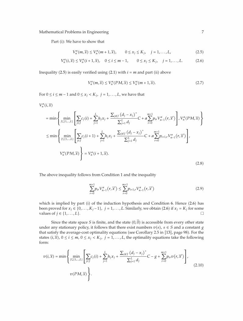
Part (i): We have to show that

V αn (m,x) ≤ V α

n (m + 1, x), 0 ≤ xj ≤ Kj, j = 1, . . . , L, (2.5)

V αn (i, x) ≤ V α

n (i + 1, x), 0 ≤ i ≤ m − 1, 0 ≤ xj ≤ Kj, j = 1, . . . , L. (2.6)

Inequality (2.5) is easily verified using (2.1) with i = m and part (ii) above

V αn (m,x) ≤ V α

n (PM,x) ≤ V αn (m + 1, x). (2.7)

For 0 ≤ i ≤ m − 1 and 0 ≤ xj < Kj, j = 1, . . . , L, we have that

V αn (i, x)

= min

⎧⎨

⎩min

J⊆{1,...,L}

⎡

⎣∑

j∈Jcj(i) +

L∑

j=1

hjxj +

∑j/∈J

(dj − xj

)+

∑Lj=1 dj

C + αm+1∑

r=0

pirVαn−1

(r, x′)

⎤

⎦, V αn (PM,x)

⎫⎬

⎭

≤ min

⎧⎨

⎩min

J⊆{1,...,L}

⎡

⎣∑

j∈Jcj(i + 1) +

L∑

j=1

hjxj +

∑j/∈J

(dj − xj

)+

∑Lj=1 dj

C + αm+1∑

r=0

pi+1,rVαn−1

(r, x′)

⎤

⎦,

V αn (PM,x)

⎫⎬

⎭= V α

n (i + 1, x).

(2.8)

The above inequality follows from Condition 1 and the inequality

m+1∑

r=0

pirVαn−1

(r, x′) ≤

m+1∑

r=0

pi+1,rVαn−1

(r, x′) (2.9)

which is implied by part (i) of the induction hypothesis and Condition 6. Hence (2.6) hasbeen proved for xj ∈ {0, . . . , Kj −1}, j = 1, . . . , L. Similarly, we obtain (2.6) if xj = Kj for somevalues of j ∈ {1, . . . , L}.

Since the state space S is finite, and the state (0, 0) is accessible from every other stateunder any stationary policy, it follows that there exist numbers v(s), s ∈ S and a constant gthat satisfy the average-cost optimality equations (see Corollary 2.5 in [13], page 98). For thestates (i, x), 0 ≤ i ≤ m, 0 ≤ xj < Kj, j = 1, . . . , L, the optimality equations take the followingform:

v(i, x) = min

⎧⎨

⎩min

J⊆{1,...,L}

⎡

⎣∑

j∈Jcj(i) +

L∑

j=1

hjxj +

∑j/∈J

(dj − xj

)+

∑Lj=1 dj

C − g +m+1∑

r=0

pirv(r, x′)

⎤

⎦,

v(PM,x)

⎫⎬

⎭.

(2.10)


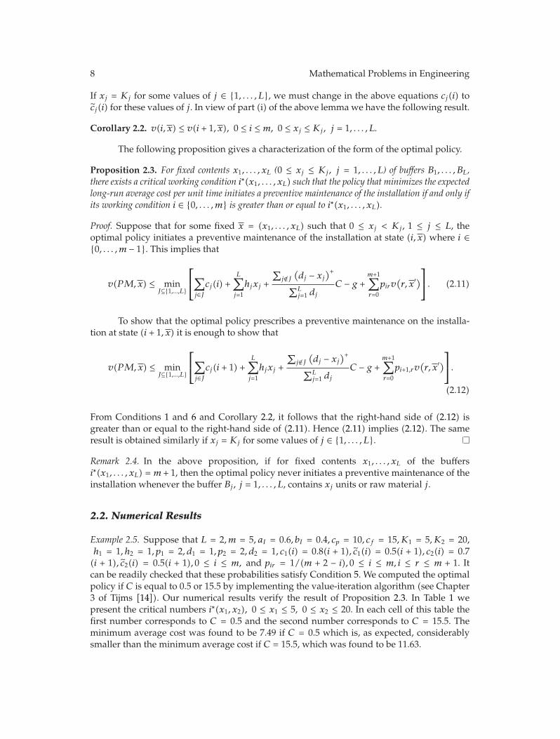
If xj = Kj for some values of j ∈ {1, . . . , L}, we must change in the above equations cj(i) toc̃j(i) for these values of j. In view of part (i) of the above lemma we have the following result.

Corollary 2.2. v(i, x) ≤ v(i + 1, x), 0 ≤ i ≤ m, 0 ≤ xj ≤ Kj, j = 1, . . . , L.

The following proposition gives a characterization of the form of the optimal policy.

Proposition 2.3. For fixed contents x1, . . . , xL (0 ≤ xj ≤ Kj, j = 1, . . . , L) of buffers B1, . . . , BL,there exists a critical working condition i∗(x1, . . . , xL) such that the policy that minimizes the expectedlong-run average cost per unit time initiates a preventive maintenance of the installation if and only ifits working condition i ∈ {0, . . . , m} is greater than or equal to i∗(x1, . . . , xL).

Proof. Suppose that for some fixed x = (x1, . . . , xL) such that 0 ≤ xj < Kj, 1 ≤ j ≤ L, theoptimal policy initiates a preventive maintenance of the installation at state (i, x) where i ∈{0, . . . , m − 1}. This implies that

v(PM,x) ≤ minJ⊆{1,...,L}

⎡

⎣∑

j∈Jcj(i) +

L∑

j=1

hjxj +

∑j/∈J

(dj − xj

)+

∑Lj=1 dj

C − g +m+1∑

r=0

pirv(r, x′)

⎤

⎦. (2.11)

To show that the optimal policy prescribes a preventive maintenance on the installa-tion at state (i + 1, x) it is enough to show that

v(PM,x) ≤ minJ⊆{1,...,L}

⎡

⎣∑

j∈Jcj(i + 1) +

L∑

j=1

hjxj +

∑j/∈J

(dj − xj

)+

∑Lj=1 dj

C − g +m+1∑

r=0

pi+1,rv(r, x′)

⎤

⎦.

(2.12)

From Conditions 1 and 6 and Corollary 2.2, it follows that the right-hand side of (2.12) isgreater than or equal to the right-hand side of (2.11). Hence (2.11) implies (2.12). The sameresult is obtained similarly if xj = Kj for some values of j ∈ {1, . . . , L}.

Remark 2.4. In the above proposition, if for fixed contents x1, . . . , xL of the buffersi∗(x1, . . . , xL) = m + 1, then the optimal policy never initiates a preventive maintenance of theinstallation whenever the buffer Bj, j = 1, . . . , L, contains xj units or raw material j.

2.2. Numerical Results

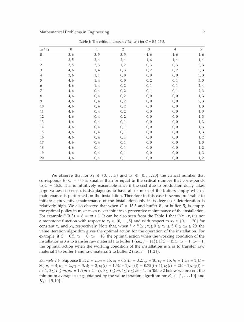
Example 2.5. Suppose that L = 2, m = 5, aI = 0.6, bI = 0.4, cp = 10, cf = 15, K1 = 5, K2 = 20,h1 = 1, h2 = 1, p1 = 2, d1 = 1, p2 = 2, d2 = 1, c1(i) = 0.8(i + 1), c̃1(i) = 0.5(i + 1), c2(i) = 0.7(i + 1), c̃2(i) = 0.5(i + 1), 0 ≤ i ≤ m, and pir = 1/(m + 2 − i), 0 ≤ i ≤ m, i ≤ r ≤ m + 1. Itcan be readily checked that these probabilities satisfy Condition 5. We computed the optimalpolicy if C is equal to 0.5 or 15.5 by implementing the value-iteration algorithm (see Chapter3 of Tijms [14]). Our numerical results verify the result of Proposition 2.3. In Table 1 wepresent the critical numbers i∗(x1, x2), 0 ≤ x1 ≤ 5, 0 ≤ x2 ≤ 20. In each cell of this table thefirst number corresponds to C = 0.5 and the second number corresponds to C = 15.5. Theminimum average cost was found to be 7.49 if C = 0.5 which is, as expected, considerablysmaller than the minimum average cost if C = 15.5, which was found to be 11.63.


Table 1: The critical numbers i∗(x1, x2) for C = 0.5, 15.5.

x2\x1 0 1 2 3 4 50 3, 6 3, 5 3, 5 4, 6 4, 6 4, 61 3, 5 2, 4 2, 4 1, 6 1, 4 1, 42 3, 5 2, 3 1, 2 0, 3 0, 3 2, 33 4, 6 1, 4 0, 3 0, 2 0, 2 3, 34 3, 6 1, 1 0, 0 0, 0 0, 0 3, 35 4, 6 1, 4 0, 0 0, 2 0, 1 3, 36 4, 6 1, 4 0, 2 0, 1 0, 1 2, 47 4, 6 0, 4 0, 2 0, 1 0, 1 2, 38 4, 6 0, 4 0, 2 0, 0 0, 0 1, 39 4, 6 0, 4 0, 2 0, 0 0, 0 2, 310 4, 6 0, 4 0, 2 0, 0 0, 0 1, 311 4, 6 0, 4 0, 2 0, 0 0, 0 1, 312 4, 6 0, 4 0, 2 0, 0 0, 0 1, 313 4, 6 0, 4 0, 1 0, 0 0, 0 1, 314 4, 6 0, 4 0, 1 0, 0 0, 0 1, 315 4, 6 0, 4 0, 1 0, 0 0, 0 1, 316 4, 6 0, 4 0, 1 0, 0 0, 0 1, 217 4, 6 0, 4 0, 1 0, 0 0, 0 1, 318 4, 6 0, 4 0, 1 0, 0 0, 0 1, 219 4, 6 0, 4 0, 1 0, 0 0, 0 1, 320 4, 6 0, 4 0, 1 0, 0 0, 0 1, 2

We observe that for x1 ∈ {0, . . . , 5} and x2 ∈ {0, . . . , 20} the critical number thatcorresponds to C = 0.5 is smaller than or equal to the critical number that correspondsto C = 15.5. This is intuitively reasonable since if the cost due to production delay takeslarge values it seems disadvantageous to have all or most of the buffers empty when amaintenance is performed on the installation. Therefore in this case it seems preferable toinitiate a preventive maintenance of the installation only if its degree of deterioration isrelatively high. We also observe that when C = 15.5 and buffer B1 or buffer B2 is empty,the optimal policy in most cases never initiates a preventive maintenance of the installation.For example i∗(0, 3) = 6 = m + 1. It can be also seen from the Table 1 that i∗(x1, x2) is nota monotone function with respect to x1 ∈ {0, . . . , 5} and with respect to x2 ∈ {0, . . . , 20} forconstant x2 and x1, respectively. Note that, when i < i∗(x1, x2), 0 ≤ x1 ≤ 5, 0 ≤ x2 ≤ 20, thevalue iteration algorithm gives the optimal action for the operation of the installation. Forexample, if C = 0.5, x1 = 0, x2 = 18, the optimal action when the working condition of theinstallation is 3 is to transfer rawmaterial 1 to buffer 1 (i.e., J = {1}). IfC = 15.5, x1 = 1, x2 = 1,the optimal action when the working condition of the installation is 2 is to transfer rawmaterial 1 to buffer 1 and raw material 2 to buffer 2 (i.e., J = {1, 2}).

Example 2.6. Suppose that L = 2, m = 15, aI = 0.3, bI = 0.2, cp = 10, cf = 15, h1 = 1, h2 = 1, C =80, p1 = 4, d1 = 2, p2 = 3, d2 = 2, c1(i) = 1.5(i + 1), c̃1(i) = 0.75(i + 1), c2(i) = 2(i + 1), c̃2(i) =i + 1, 0 ≤ i ≤ m, pir = 1/(m + 2 − i), 0 ≤ i ≤ m, i ≤ r ≤ m + 1. In Table 2 below we present theminimum average cost g obtained by the value-iteration algorithm for K1 ∈ {1, . . . , 10} andK2 ∈ {5, 10}.


Table 2: The minimum average cost as K1 or K2 varies.

K1 K2 = 5 K2 = 101 51.20 51.172 48.55 48.493 47.55 47.504 45.94 45.885 45.60 45.566 44.87 44.837 44.78 44.758 44.49 44.459 44.46 44.4310 44.39 44.37

From the above table we see that as K1 or K2 increases, the minimum average costdecreases. This is intuitively reasonable because in this example it seems favourable to havebuffers with large, capacities since the cost rate C due to production delay is relatively largewhile the probabilities aI , bI of successful maintenances and the storage cost rates h1, h2 arerelatively small.

3. The Problem when the Production Unit Deteriorates Stochastically

We consider the same production-inventory system (see Figure 1) as the one introduced in theprevious section with the following modifications: (i) the installation is always in operativecondition while the production unit may experience a failure as time evolves and (ii) as longas the buffer Bj, j = 1, . . . , L, is not empty and the production unit is in operative condition,the production unit may pull the raw material j from buffer Bj at a constant rate of dj(> pj)units of raw material j per unit of time. When the buffer Bj is empty and the production unitis in operative condition, the production unit reduces its pull rate from dj to pj .

We assume that the production unit is monitored at discrete equidistant time epochsτ = 0, 1, . . . (say every day), and is classified into one of n+2working conditions 0, . . . , n+1.Wesuppose that working condition i is better than working condition i + 1. Working condition0 means that the production unit is new (or functioning as good as new), while workingcondition n + 1 means that the production unit does not function, and it cannot pull thematerials from the buffers. The intermediate working conditions 1, . . . , n are operative. If theworking condition at time epoch τ is i then the working condition at time epoch τ + 1 willbe r with probability qir . The probability that the deterioration process of the production unitreaches eventually the failure state n + 1 from any initial working condition i is assumedto be nonzero. If at a time epoch τ the production unit is found to be at the failure staten + 1, a corrective maintenance is compulsory. If it is found to be at any working conditioni ≤ n, a preventive maintenance is optional. The production unit does not operate when it isunder preventive maintenance, and it does not pull any raw material from its buffer. When apreventive or a corrective maintenance is performed and the buffer Bj, j = 1, . . . , L, containsxj units of raw material j, the installation transfers min(pj ,Kj − xj) units of raw materialj to buffer Bj during one unit of time. The preventive and corrective maintenance times(expressed in time units) are geometrically distributed with probability of success aP and bP ,respectively. Both maintenances bring the production unit to its perfect condition 0. The statespace of the system is the set S̃ = {0, . . . , n+ 1, PM}×{0, . . . , K1}× · · · × {0, . . . , KL}, where PMrepresents the situation that the production unit is under a preventive repair. The possible


actions are the same as the ones considered in the problem studied in Section 2 with thefollowing modification: action J ⊆ {1, . . . , L} is the action of pulling raw materials only frombuffers Bj, j ∈ J . If at a time epoch τ the production unit is found to be at working conditioni ∈ {0, . . . , n}, then we may choose either the action of initiating a preventive maintenance oraction J ⊆ {1, . . . , L}.

The cost structure includes operating costs of the production unit, storage costs,maintenance costs, costs due to production delay, and penalty costs. The storage costshj , j ∈ {1, . . . , L}, and the maintenance costs cp, cf are defined exactly in the same way as inthe problem studied in the previous section. If the working condition of the production unitis i ∈ {0, . . . , n} and the buffer Bj, j ∈ {1, . . . , L}, is nonempty (or empty), the cost of pullingdj (or pj) units of raw material j from buffer Bj during one unit of time is equal to cj(i) (orc̃j(i)). We assume that the cost rate due to production delay as long as a maintenance of theproduction unit lasts is equal to C > 0. Therefore, if at a time epoch τ the action J ⊆ {1, . . . , L}is selected and the content of buffer Bj, j = 1, . . . , L, is xj ∈ {0, . . . , Kj}, then the cost due toproduction delay until time epoch τ + 1 is equal to C(

∑j/∈J dj +

∑j∈J(dj − pj − xj)

+)/∑L

j=1 dj,

where (dj − pj − xj)+ = max(dj − pj − xj , 0) is the unavailable quantity of raw material j ∈ J

during one unit of time. A penalty cost per unit time which is equal to Pj > 0, j = 1, . . . , L, isalso imposed for each unit or raw material j that is not stored in buffer Bj during a correctiveor a preventive maintenance of the production unit when the buffer Bj is full. This cost isdue to the necessary labor for transferring and storing the raw material in another place untilthe completion of the maintenance. We assume that Conditions 1–5 on the cost structure thatwe introduced for the problem studied in the previous section are valid if we replace bI withbP , aI with aP , and m with n. We consider a discrete-time Markov decision process in whichwe aim to find a stationary policy which minimizes the expected long-run average cost perunit of time. Note that for L = 1, the problem was studied in Pavitsos and Kyriakidis [2].

Since the state space S̃ is finite and the state (0, K1, . . . , KL) is accessible from everyother state under any stationary policy, it follows that there exist numbers w(s), s ∈ S anda constant g that satisfy the average-cost optimality equations. For the states (i, x), 0 ≤ i ≤n, 0 < xj ≤ Kj , j = 1, . . . , L, the optimality equations have the following form:

w(i, x) = min{

minJ⊆{1,...,L}

A(J), w(PM,x)}

, (3.1)

where

A(J) =∑

j∈Jcj(i) +

L∑

j=1

hjxj +

∑j/∈J dj +

∑j∈J

(dj − pj − xj

)+

∑Lj=1 dj

C

+∑

j/∈JPj

(pj + xj −Kj

)+ − g +m+1∑

r=0

qirw(r, x′),

(3.2)

w(PM,x) =L∑

j=1

hjxj + C +L∑

j=1

Pj

(pj + xj −Kj

)+

− g + aPw(0,min

(x1 + p1, K1

), . . . ,min

(xL + pL,KL

))

+ (1 − aP )w(PM,min

(x1 + p1, K1

), . . . ,min

(xL + pL,KL

)).

(3.3)


If xj = 0 for some values of j ∈ {1, . . . , L}, we must change in (3.2) cj(i) to c̃j(i) for thesevalues. Note that x′ in (3.2) is a vector with L components in which the jth component isequal to (xj + pj − dj)

+ if j ∈ J , while, if j /∈ J , it is equal to (xj − dj)+. It is possible to

prove that w(i, x) ≤ w(i + 1, x), 0 ≤ i ≤ n, 0 ≤ xj ≤ Kj, j = 1, . . . , L, using the dynamicprogramming equation for the corresponding finite-horizon problem. The method is exactlythe same as that used for the proof of Corollary 2.2 in the previous section and, therefore,we omit the details. An immediate consequence of the above monotonicity result is that theresult of Proposition 2.3 is valid for the problem of the optimal preventive maintenance of theproduction unit.

3.1. Numerical Examples

Example 3.1. Suppose that L = 2, K1 = 7, K2 = 10, n = 10, aP = 0.6, bP = 0.4, cp = 0.4, cf =0.8, h1 = 1, h2 = 2, C = 0.5, P1 = 1, P 2 = 1, p1 = 1, d1 = 2, p2 = 1, d2 = 2, c1(i) = 2(i +1), c̃1(i) = 1.5(i + 1), c2(i) = 3(i + 1), c̃2(i) = 2.5(i + 1), 0 ≤ i ≤ n, and pir = 1/(n + 2 − i), 0 ≤i ≤ n, i ≤ r ≤ n + 1. We computed the optimal policy by implementing the value-iterationalgorithm. Theminimum average cost was found to be 15.67. In Table 3, we present the criticalnumbers i∗(x1, x2), 0 ≤ x1 ≤ 7, 0 ≤ x2 ≤ 10.

We can see from Table 3 that i∗(x1, x2) is not a monotone function with respect to x1 ∈{0, . . . , 7} or with respect to x2 ∈ {0, . . . , 10}, respectively. Note that, when i < i∗(x1, x2), 0 ≤x1 ≤ 7, 0 ≤ x2 ≤ 10, the value-iteration algorithm gives the optimal action for the operationof the production unit. For example, if x1 = 0, x2 = 9, the optimal action when the workingcondition of the installation is i ∈ {0, 1, 2, 3, 4} is to pull rawmaterial 1 from buffer B1 and rawmaterial 2 from buffer B2 (i.e., J = {1, 2}), while, when the working condition is i ∈ {5, 6, 7}the optimal condition is to pull only raw material 2 from buffer B2 (i.e., J = {2}).

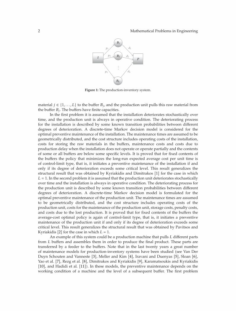
Example 3.2. Suppose that L = 2, K1 = 5, K2 = 15, n = 10, a = 0.6, b = 0.4, cp = 0.5, cf =0.8, C = 0.5, P 1 = 1, P2 = 1, p1 = 1, d1 = 2, p2 = 1, d2 = 2, c1(i) = 2(i + 1), c̃1(i) = 1.5(i +1), c2(i) = 3(i + 1), c̃2(i) = 2.5(i + 1), 0 ≤ i ≤ n, and pir = 1/(n + 2 − i), 0 ≤ i ≤ n, i ≤ r ≤n + 1. In Figure 2 we present the graph of the minimum average cost g(h1) as a function ofh1 ∈ {1, . . . , 10}, if h2 = 1, and the graph of the minimum average cost g(h2) as a function ofh2 ∈ {1, . . . , 10}, if h1 = 1. We observe that g(hi), i = 1, 2, increases as hi increases. The increaseof the minimum average cost is more intense when h2 increases. This can be explained by thefact that the capacity of buffer B2 is considerably greater than the capacity of buffer B1.

4. Conclusions and Future Research

We presented two discrete-time Markov decision models for the optimal condition-basedpreventive maintenance of a production system which consists of two machines and Lintermediate buffers. The first machine transfers L different raw materials to the buffers,and the second machine draws the raw materials from the buffers. The second machine isconsidered to be a production unit that assembles the raw materials in order to producethe final product. In the first model, it is assumed that only the first machine deterioratesstochastically over time while the production unit is always in operative condition. It ispossible to monitor the first machine at discrete equidistant time epochs and to classify itinto one working condition that describes its level of deterioration. If the first machine is


Table 3: The critical numbers i∗(x1, x2), 0 ≤ x1 ≤ 7, 0 ≤ x2 ≤ 10.

x2\x1 0 1 2 3 4 5 6 70 2 6 7 7 7 6 4 21 8 9 9 9 9 9 8 82 9 10 10 10 10 10 9 93 10 10 10 10 10 10 10 14 10 10 10 10 10 10 10 105 10 10 10 10 10 10 10 106 10 10 10 10 10 10 10 107 10 10 10 10 10 10 10 108 10 10 10 10 10 10 10 109 8 8 9 9 9 9 9 910 3 4 4 5 5 5 4 3

35

30

25

20

15

10

Min

imum

ave

rage

cos

tg

1 2 3 4 5 6 7 8 9 10

Holding costs h1 and h2

g(h1)g(h2)

Figure 2: The minimum average cost g(h1) and g(h2).

in failed condition a corrective maintenance must be commenced; otherwise a preventivemaintenance may be performed or the action of transferring raw materials to any subset ofthe set of L buffers may be selected. The maintenances bring the first machine to its perfectcondition. In the second model it is assumed, that only the production unit deteriorates overtime, and the first machine is always in operative machine. It is possible to determine the levelof deterioration of the production unit after inspecting it at discrete equidistant time epochs. Ifthe production unit is in failed condition a corrective maintenance must be started; otherwisea preventive maintenance may be initiated or the action of pulling the raw materials fromany subset of the set of L buffers may be selected. Both maintenances bring the productionunit to its perfect condition.

In both models we considered the problem of determining the policy that minimizesthe expected long-run average cost per unit time. If the maintenance times are geometricallydistributed we proved that, in both models, the optimal policy is of control-limit type, that is,


for fixed contents of the buffers it prescribes a preventive maintenance of the first machine orthe production unit if and only if its degree of deterioration exceeds some critical level. Theproof was achieved through the corresponding finite-horizon problem.

A topic for future research could be a more complicated problem in which the firstmachine transfers the raw materials to the buffers and the production unit draws them fromthe buffers in a random manner. Another topic for future research could be the study of themaintenance problems that we would have if the maintenance times are not geometricallydistributed but follow some general distributions with suitable conditions.

Acknowledgment

The authors would like to thank an anonymous referee for helpful comments.

References

[1] E. G. Kyriakidis and T. D. Dimitrakos, “Optimal preventive maintenance of a production systemwithan intermediate buffer,” European Journal of Operational Research, vol. 168, no. 1, pp. 86–99, 2006.

[2] A. Pavitsos and E. G. Kyriakidis, “Markov decision models for the optimal maintenance of a pro-duction unit with an upstream buffer,”Computers and Operations Research, vol. 36, no. 6, pp. 1993–2006,2009.

[3] F. A. van der Duyn Schouten and S. G. Vanneste, “Maintenance optimization of a production systemwith buffer capacity,” European Journal of Operational Research, vol. 82, no. 2, pp. 323–338, 1995.

[4] R. D. Meller and D. S. Kim, “The impact of preventive maintenance on system cost and buffer size,”European Journal of Operational Research, vol. 95, no. 3, pp. 577–591, 1996.

[5] S. M. R. Iravani and I. Duenyas, “Integrated maintenance and production control of a deterioratingproduction system,” IIE Transactions, vol. 34, no. 5, pp. 423–435, 2002.

[6] T. W. Sloan, “A periodic review production and maintenance model with random demand, deteri-orating equipment, and binomial yield,” Journal of the Operational Research Society, vol. 55, no. 6, pp.647–656, 2004.

[7] X. Yao, X. Xie, M. C. Fu, and S. I. Marcus, “Optimal joint preventive maintenance and productionpolicies,” Naval Research Logistics, vol. 52, no. 7, pp. 668–681, 2005.

[8] N. Rezg, A. Chelbi, and X. Xie, “Modeling and optimizing a joint inventory control and preventivemaintenance strategy for a randomly failing production unit: analytical and simulation approaches,”International Journal of Computer Integrated Manufacturing, vol. 18, no. 2-3, pp. 225–235, 2005.

[9] T. D. Dimitrakos and E. G. Kyriakidis, “A semi-Markov decision algorithm for the maintenanceof a production system with buffer capacity and continuous repair times,” International Journal ofProduction Economics, vol. 111, no. 2, pp. 752–762, 2008.

[10] C. C. Karamatsoukis and E. G. Kyriakidis, “Optimal maintenance of a production-inventory systemwith idle periods,” European Journal of Operational Research, vol. 196, no. 2, pp. 744–751, 2009.

[11] L. A. Hadidi, U. M. Al-Turki, and A. Rahim, “Integrated models in production planning and sched-uling, maintenance and quality: a review,” International Journal of Industrial and Systems Engineering,vol. 10, no. 1, pp. 21–50, 2012.

[12] C. Derman, Finite State Markovian Decision Processes, Mathematics in Science and Engineering, Aca-demic Press, New York, NY, USA, 1970.

[13] S. Ross, Introduction to Stochastic Dynamic Programming, Probability and Mathematical Statistics, Aca-demic Press, New York, NY, USA, 1983.

[14] H. C. Tijms, Stochastic Models: An Algorithmic Approach, Wiley Series in Probability and MathematicalStatistics: Applied Probability and Statistics, John Wiley & Sons, Chichester, UK, 1994.

Submit your manuscripts athttp://www.hindawi.com

Hindawi Publishing Corporationhttp://www.hindawi.com Volume 2014

MathematicsJournal of


Mathematical Problems in Engineering

Hindawi Publishing Corporationhttp://www.hindawi.com

Differential EquationsInternational Journal of

Volume 2014

Applied MathematicsJournal of


Probability and StatisticsHindawi Publishing Corporationhttp://www.hindawi.com Volume 2014

Journal of


Mathematical PhysicsAdvances in

Complex AnalysisJournal of


OptimizationJournal of


CombinatoricsHindawi Publishing Corporationhttp://www.hindawi.com Volume 2014

International Journal of


Operations ResearchAdvances in

Journal of


Function Spaces

Abstract and Applied AnalysisHindawi Publishing Corporationhttp://www.hindawi.com Volume 2014

International Journal of Mathematics and Mathematical Sciences


The Scientific World JournalHindawi Publishing Corporation http://www.hindawi.com Volume 2014


Algebra

Discrete Dynamics in Nature and Society



Decision SciencesAdvances in

Discrete MathematicsJournal of

Hindawi Publishing Corporationhttp://www.hindawi.com

Volume 2014 Hindawi Publishing Corporationhttp://www.hindawi.com Volume 2014

Stochastic AnalysisInternational Journal of

Documents

Optimal Maintenance of a Production System with L