Embed Size (px)
Citation preview

PHYSICAL REVIEW D 70, 022003 ~2004!
brought to you by COREView metadata, citation and similar papers at core.ac.uk
provided by Caltech Authors - Main
Optimal filtering of the LISA data
Andrzej Krolak,* Massimo Tinto,† and Michele Vallisneri‡
Jet Propulsion Laboratory, California Institute of Technology, Pasadena, California 91109, USA~Received 19 January 2004; published 26 July 2004!
The LISA time-delay-interferometry responses to a gravitational wave signal are rewritten in a form thataccounts for the motion of the LISA constellation around the Sun; the responses are given in closed analyticforms valid for any frequency in the band accessible to LISA. We then present a complete procedure, based onthe principle of maximum likelihood, to search for stellar-mass binary systems in the LISA data. We define therequired optimal filters, the amplitude-maximized detection statistic~analogous to theF statistic used in pulsarsearches with ground-based interferometers!, and discuss the false-alarm and detection probabilities. We thentest the procedure in numerical simulations of gravitational-wave detection.
DOI: 10.1103/PhysRevD.70.022003 PACS number~s!: 95.55.Ym, 04.80.Nn, 95.75.Pq, 97.60.Gb
vitb
tifion
erco
e-eeesn
it-rarae
one
l
icveoa
yD
tors
e-ivee-, atl ofangaserro-
Ay
as
rens,theyusebyla-foronce
ob-ingof
onheth
po-first
rro-thes
tted
es
tes
I. INTRODUCTION
The Laser Interferometer Space Antenna~LISA! is adeep-space mission aimed at detecting and studying grational radiation in the millihertz frequency band. A joinAmerican and European project, it is expected tolaunched in the year 2011, and to start collecting sciendata approximately a year later, after reaching its orbital cfiguration of operation@1#. LISA consists of three widelyseparated spacecraft, flying in a triangular, almost equilatconfiguration, and exchanging coherent laser beams. Intrast to ground-based, equal-arm gravitational-wave~GW!interferometers, LISA will have multiple readouts, corrsponding to the six laser Doppler shifts measured betwspacecraft. Modeling each spacecraft as carrying lasbeam splitters, photodetectors, and drag-free proof masseeach of two optical benches, Armstrong, Estabrook, aTinto @2–4# showed that it is possible to combine, with suable time delays, the six time series of the inter-spacecDoppler shifts and the six time series of the intra-spacecDoppler shifts~measured between adjacent optical bench!to cancel the otherwise overwhelming frequency fluctuatiof the lasers (Dn/n.10213/AHz), and the noise due to thmechanical vibrations of the optical benches~which could beas large asDn/n.10216/AHz). The strain sensitivity levethat then becomes achievable,h.10221/AHz, is set by thebuffeting of the drag-free proof masses inside each optbench, and by the shot noise at the photodetectors. Sesuch laser-noise-free interferometric combinations are psible, and they show different couplings to gravitationwaves and to the remaining system noises@2–5#. The tech-nique used to synthesize these combinations is knowntime-delay interferometry~TDI!; in the case of a stationararray, it was shown that the space of all the possible T
*Also at Institute of Mathematics, Polish Academy of SciencWarsaw, Poland. Electronic address: [email protected]
†Also at Space Radiation Laboratory, California Instituof Technology, Pasadena, CA 91125. Electronic [email protected]
‡Electronic address: [email protected]
0556-2821/2004/70~2!/022003~24!/$22.50 70 0220
ta-
ec-
aln-
nrs,ond
ftftss
alrals-l
as
I
observables can be constructed by combining four genera@2,6#.
Recently, it was pointed out@7–10# that the rotationalmotion of the LISA array around the Sun and the time dpendence of light travel times introduced by the relat~shearing! motion of the spacecraft have the effect of prventing the suppression of laser frequency fluctuationsleast under the current stability requirements, to the levethe secondary noisesin the TDI observables as derived forstationary array. This problem was addressed by devisinew combinations that are capable of suppressing the lfrequency fluctuations below the secondary noises for atating LISA array@7,8#, and for a rotating and shearing LISarray @9,10#. In this context, the original stationary-arracombinations are sometimes known as ‘‘TDI 1.0’’~or first-generation TDI!, the rotating-LISA combinations as ‘‘TDI1.5,’’ and the rotating and shearing-LISA combinations‘‘TDI 2.0;’’ following Ref. @10#, we refer to the last assecond-generationTDI. Second-generation combinations aessentially finite differences of first-generation combinatioand as such they appear more complicated. However,retain the same sensitivity to incoming GWs: this is becathe corrections introduced in the original combinationsthe changing array geometry are obviously important forser frequency fluctuations, but they are negligibly smallthe GW responses and for the secondary noises; thus,laser frequency noise is removed, the second-generationservables become finite differences of the correspondfirst-generation observables. At a fixed frequency, the ratioGW response to secondary noises~and hence the sensitivity!is then unchanged.
The GW responses of the TDI combinations dependthe relative orientation of the LISA array with respect to tdirection of propagation of the GW signal, on the strengand polarization of the signal, and on its frequency comnents. Analytic expressions for the TDI responses werederived by Armstrong, Estabrook and Tinto@2#, for a station-ary LISA array. A realistic model of LISA must howeveinclude the motion of the array around the Sun, which intduces slow modulations in the phase and amplitude ofGW responses~in addition, of course, to the modificationintroduced by adopting second-generation TDI!. For in-stance, the LISA responses to the sinusoidal signal emi
,
s:
©2004 The American Physical Society03-1

sTctudaays
ndbys
ootesv
-en
wnpmeo
ve
reioidleininnafreste
a
atoio
erkr
-
onen
. Iigtoruist
ithlse-
toah-ndo-s. In
raftx of2
iveraft,
redce-
ion
be-hese
m-
bytics,
y.n
ace-
la-hes,dft.
ri-
KROLAK, TINTO, AND VALLISNERI PHYSICAL REVIEW D 70, 022003 ~2004!
by a binary system are not simple sinusoids, but ratherperpositions of many sinusoids of smaller amplitude.maximize the likelihood of source detection, these effemust be modeled in GW search algorithms, either by incling the modulations in the theoretical models of the sign~i.e., thetemplates!, or by demodulating the LISA data forgiven set of sky positions as the first step of data anal@11,12#.
In this paper we derive the response of the secogeneration TDI observables to the GW signals generatedbinary system, and we describe how signal templates baon these responses can be used in a maximum-likelihmatched-filtering framework to search for binaries andestimate their parameters once they are found. Other mods to analyze the LISA data for signals from binarieimplemented in the long-wavelength approximation, habeen proposed in Refs.@13,14#. We work in the solar-systembaricentric frame, and we follow closely the derivation givby Jaranowski, Kro´lak, and Schutz@15# for continuoussources and ground-based detectors. A similar formalismused by Giampieri@16# to obtain the antenna pattern of aarbitrary orbiting interferometer, in the long-wavelength aproximation. The response of an orbiting equal-arMichelson interferometer to a sinusoidal signal was workout by Cutler@17#, again in the long-wavelength limit. Set@18# extended Cutler’s formalism to high frequencies~and tonoise-canceling observables!, in the context of studyingoptimal-filtering parameter estimation for supermassiblack-hole binaries. Cornish, Rubbo, and Poujade@19,20#obtained general expressions valid in the entire LISA fquency band, and for arbitrary GW signals; these expressare given as integrals over the LISA arms, and they provthe basic building blocks to assemble the TDI observabBy contrast, in this paper we work out explicit time-domaexpressions for the LISA response to moderately chirpbinary systems, for all the second-generation TDI combitions. These expressions are valid over the entire LISAquency band, and they are written as linear combinationfour time-dependent functions; this linear structure facilitathe computation of matched filters and the design of optimfiltering algorithms.
This paper is organized as follows. In Sec. II we givebrief overview of the derivation of the TDI responsesGWs for a stationary array, and we argue that the correctintroduced by the motion of the LISA array and by the timdependence of light travel times are negligibly small. Woing in the solar-system-baricentric frame, we obtain geneexpressions for the GW responses of the Michelson (X1 , X2 ,X3), Sagnac (a1 , a2 , a3), and optimal (A, E, T; see@21#!second-generation TDI observables~expressions for the firstgeneration observables are given in Appendix C!; finally, wederive the corresponding closed-form analytic expressifor moderately chirping binary systems, valid at any frquency in the LISA band. In Sec. III we provide expressiofor the spectral densities of noise in the TDI combinationsSec. IV we combine the results of Secs. II and III to desoptimal filters that can be applied to the LISA TDI datasearch for binary stars; we take advantage of the linear stture of the responses to define an optimal detection statthat does not depend on the effective polarization and on
02200
u-os-
ls
is
-a
edd,
oth-,e
as
--d
-
-nses.
g--
ofsl
ns
-al
s-snn
c-tiche
initial phase of the binary, in analogy to theF statistic@15,22# used in searches for continuous GW sources wground-based interferometers. In Sec. V we derive the faalarm and false-dismissal probabilities for our LISAF sta-tistic. Last, in Sec. 6 we describe an efficient algorithmcomputeF, and we implement it numerically; we performsimulation of GW detections in both the low and higfrequency part of the LISA band, and for both Michelson aoptimal @21# TDI observables, and we show that our algrithm yields very accurate estimates of source parameterthe rest of this paper we shall use units wherec51.
II. TIME-DELAY INTERFEROMETRY
Figure 1 shows the overall LISA geometry. The spacecare labeled 1, 2, and 3; the arms are labeled with the indethe opposite spacecraft~e.g., arm 1 lies between spacecraftand 3!. The light travel time~or, loosely, thearmlength!along armi is denoted byLi @7–10#. The basic constituentsof the TDI observables are the time series of the relatlaser-frequency fluctuations measured between spacecwhich are denoted byyi j (t), with iÞ j : for instance,y31(t) isthe time series of relative frequency fluctuations measufor reception at spacecraft 1 with transmission from spacraft 3 ~along arm 2!; similarly, y21(t) is the time seriesmeasured for reception at spacecraft 1 with transmissfrom spacecraft 2~along arm 3!, and so on. Six more timeseries result from comparing the laser beams exchangedtween adjacent optical benches within each spacecraft; ttime series are denoted byzi j , with i , j 51,2,3, iÞ j ~see@3,4,10# for details!. Delayed time series are denoted by comas: for instance,y31,25y31@ t2L2(t)#, and so on.
The frequency fluctuations introduced by the lasers,the optical benches, by the proof masses, by the fiber opand by the measurement itself at the photo-detector~i.e., theshot-noise fluctuations! enter the Doppler observablesyi jandzi j with specific time signatures; see Refs.@3,4,10# for adetailed discussion. The contributionyi j
GW due to GW signalswas derived in Ref.@2# in the case of a stationary arra~Note that in Ref.@2#, and indeed in all the literature ofirst-generation TDI, the notationyi j indicates the one-wayDoppler measurement for the laser beam received at sp
FIG. 1. Schematic LISA configuration. The spacecraft arebeled 1, 2, and 3; each spacecraft contains two optical bencdenoted by 1,1* , . . . , asindicated. The optical paths are denoteby Li , where the indexi corresponds to the opposite spacecra
The unit vectorsni point between pairs of spacecraft, with the oentation indicated.
3-2
ro
acste
thdetha
tinnle
ise
ee
mawtilauns
thI C
ereeral-
eric
set
teSB
-onaft
r-rie
OPTIMAL FILTERING OF THE LISA DATA PHYSICAL REVIEW D 70, 022003 ~2004!
craft j andtraveling along arm i. In this paper we conform tothe notation used in Refs.@7–10#.!
Since the motion of the LISA array around the Sun intduces a difference between~and a time dependence in! thecorotating and counterrotating light travel times, the exexpressions for the GW contributions to the various firgeneration TDI combinations will in principle differ from thexpressions valid for a stationary array@2#. However, themagnitude of the corrections introduced by the motion ofarray are proportional to the product between the timerivative of the GW amplitude and the difference betweenactual light travel times and those valid for a stationary arrAt 1 Hz, for instance, the larger correction to the signal~dueto the difference between the corotating and counterrotalight travel times! is two orders of magnitude smaller thathe main signal. Since the amplitude of this correction scalinearly with the Fourier frequency, we can completely dregard this effect~and the weaker effect due to the timdependence of the light travel times! over the entire LISAband@10#. Furthermore, since along the LISA orbit the thrarmlengths will differ at most by;1% –2%, the degradationin signal-to-noise ratio introduced by adopting signal teplates that neglect the inequality of the armlengths will bemost a few percent. For these reasons, in what followsshall derive the GW responses of various second-generaTDI observables by disregarding the differences in the detimes experienced by light propagating clockwise and coterclockwise, and by assuming the three LISA armlengthbe constant and equal toL553106 km.16.67 s @23#.These approximations, together with the treatment ofmoving-LISA GW response discussed at the end of Sec. Iare essentially equivalent to therigid adiabatic approxima-tion of Ref. @20#, and to the formalism of Ref.@18#.
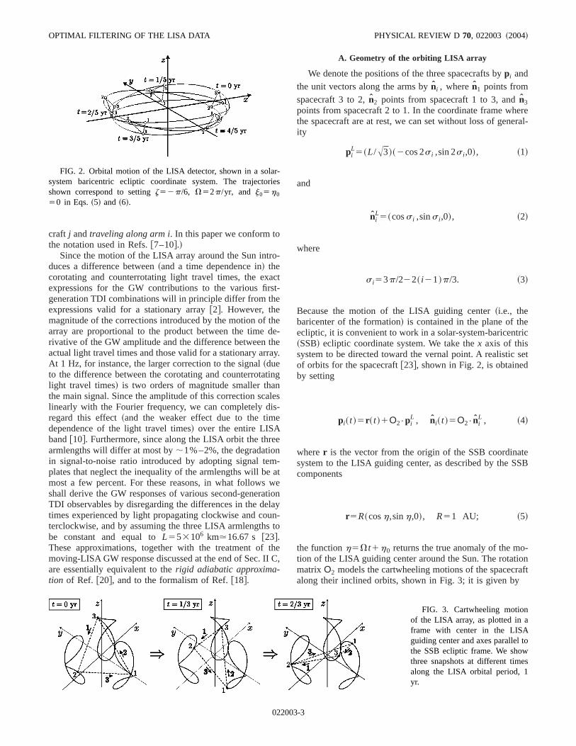
FIG. 2. Orbital motion of the LISA detector, shown in a solasystem baricentric ecliptic coordinate system. The trajectoshown correspond to settingz52p/6, V52p/yr, and j05h0
50 in Eqs.~5! and ~6!.
02200
-
t-
e-
ey.
g
s-
-teony-
to
e,
A. Geometry of the orbiting LISA array
We denote the positions of the three spacecrafts bypi andthe unit vectors along the arms byni , wheren1 points fromspacecraft 3 to 2,n2 points from spacecraft 1 to 3, andn3points from spacecraft 2 to 1. In the coordinate frame whthe spacecraft are at rest, we can set without loss of genity
piL5~L/A3!~2cos 2s i ,sin 2s i ,0!, ~1!
and
niL5~coss i ,sins i ,0!, ~2!
where
s i53p/222~ i 21!p/3. ~3!
Because the motion of the LISA guiding center~i.e., thebaricenter of the formation! is contained in the plane of thecliptic, it is convenient to work in a solar-system-baricent~SSB! ecliptic coordinate system. We take thex axis of thissystem to be directed toward the vernal point. A realisticof orbits for the spacecraft@23#, shown in Fig. 2, is obtainedby setting
pi~ t !5r ~ t !1O2•piL , ni~ t !5O2•ni
L , ~4!
wherer is the vector from the origin of the SSB coordinasystem to the LISA guiding center, as described by the Scomponents
r5R~cosh,sinh,0!, R51 AU; ~5!
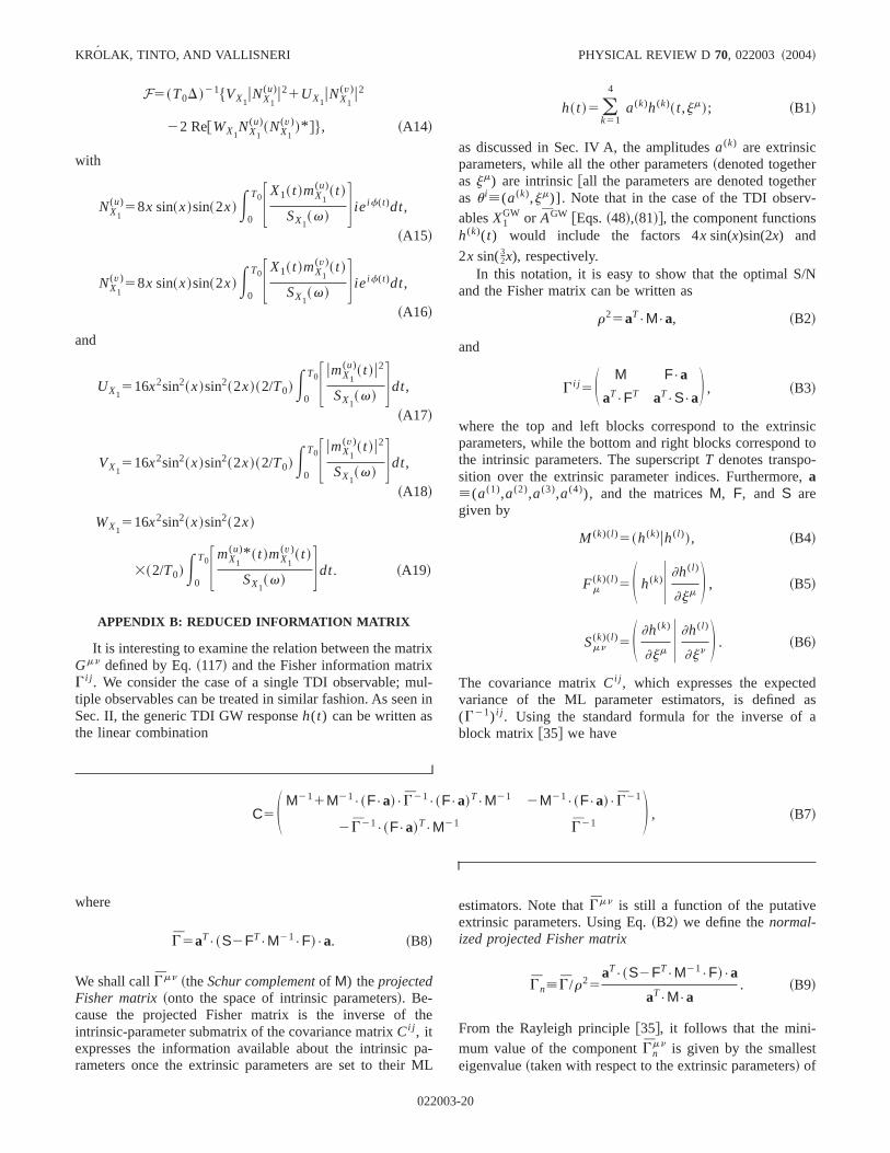
the functionh5Vt1h0 returns the true anomaly of the motion of the LISA guiding center around the Sun. The rotatimatrix O2 models the cartwheeling motions of the spacecralong their inclined orbits, shown in Fig. 3; it is given by
s
o
s
FIG. 3. Cartwheeling motionof the LISA array, as plotted in aframe with center in the LISAguiding center and axes parallel tthe SSB ecliptic frame. We showthree snapshots at different timealong the LISA orbital period, 1yr.
3-3

,by
de
KROLAK, TINTO, AND VALLISNERI PHYSICAL REVIEW D 70, 022003 ~2004!
O25S sinh cosj2cosh sinz sinj 2sinh sinj2cosh sinz cosj 2cosh cosz
2cosh cosj2sinh sinz sinj cosh sinj2sinh sinz cosj 2sinh cosz
cosz sinj cosz cosj 2sinzD ; ~6!
the functionj52Vt1j0 returns the phase of the motion of each spacecraft around the guiding center, whilez sets theinclination of the orbital plane with respect to the ecliptic. For the LISA trajectory,V52p/yr and z52p/6 @23#. Forsimplicity, we can seth05j050, so that at timet50 the LISA guiding center lies on the positivex axis of the SSB systemwhile p1 lies on the negativey axis. The spacecraft orbits described by Eq.~4! can be approximately mapped to those usedCornish and Rubbo@19# by identifying our spacecraft 1, 2, and 3 with their spacecraft 0, 2, and 1, and by settingh05k,j053p/22k1l, wherek andl are the parameters defined below Eqs.~56! and ~57! of Ref. @19#.
B. Generic plane waveform
At the origin of the SSB frame, the transverse-traceless metric perturbation due to a source located at ecliptic latitub andlongitudel can be written as
H~ t !5O1•HS~ t !•O121 , ~7!
where the metric perturbation in the source frame is taken to be
HS~ t !5S h1~ t ! h3~ t ! 0
h3~ t ! 2h1~ t ! 0
0 0 0D , ~8!
with h1(t) andh3(t) the two GW polarizations, and where
O15S sinl cosc2cosl sinb sinc 2sinl sinc2cosl sinb cosc 2cosl cosb
2cosl cosc2sinl sinb sinc cosl sinc2sinl sinb cosc 2sinl cosb
cosb sinc cosb cosc 2sinbD ; ~9!
p
c-o
ee
mheieinbyaa
e
rom
the dependence of the rotation matrixO1 on b and l en-forces the transversality of the plane waves, which are progating from a source located in the direction
k5~cosl cosb,sinl cosb,sinb!; ~10!
the polarization anglec encodes a rotation around the diretion of wave propagation,2 k, setting the convention used tdefine the two polarizations,1 and 3. The polarizationscorresponding toc50 are shown in Fig. 4 for various sourcpositions in the sky. In the center of the LISA proper fram~the frame where the spacecraft are at rest!, the transverse-traceless metric perturbation is given by
HL~ t !5O221~ t !O1HS~ t !O1
21O2~ t !. ~11!
The time variablet that appears inh1(t) and h3(t) @andtherefore inH(t) andHL(t)] is the time at the origin of theSSB frame. It is related to the time in the GW source fraby a relativistic time dilation, due to the proper motion of tsource and to cosmological effects. It is however expedto identify the two times, and to describe GW emission usSSB time; the time dilation is then taken into accountmapping the apparent~measured! physical parameters ofsource into its real parameters. The source positional par
02200
a-
e
ntg
m-
etersb, l, and c can be mapped to the parametersu, f,and c used in Ref.@19# by settingb5p/22u, l5f, andc52c.
C. GW response of the LISA array
As derived in Ref.@2# for a stationary, equilateral-trianglLISA array, the one-way Doppler responsesy21 andy31 ex-cited by a plane transverse-traceless GW propagating fthe source directionk, are given by
FIG. 4. Conventional definition of the GW polarizations1~dashed! and 3 ~solid! for various ecliptic latitudesb and longi-tudesl.
3-4

f
e
naoum
ng
h
f
e-1/ucbS
ry
am
n
ns
eofew-
p-nifi-nal;eds
,neder
t atillies50
le.toin
fi-
ndult-
OPTIMAL FILTERING OF THE LISA DATA PHYSICAL REVIEW D 70, 022003 ~2004!
y21GW~ t !5@12 k•n3#@C3~ t1 k•p22L !2C3~ t1 k•p1!#,
~12!
y31GW~ t !5@11 k•n2#@C2~ t1 k•p32L !2C2~ t1 k•p1!#
~13!
@in the notation of Ref.@2#, oury21, y31, andk correspond toy31, y21, and2 k, respectively# where
C j~ t !5F j~ t !
12~ k•nj !2
, F j~ t !51
2nj8•H~ t !•nj ~14!
@the prime denotes vector transposition#. The twoC i termsin each of Eqs.~12! and ~13! correspond to the events oemission~at spacecraft 2 and 3, respectively! and reception~at spacecraft 1! of a laser photon packet; the time of themission event is therefore retarded by an armlengthL. Thek•pi terms represent the retardation of the gravitatiowavefronts to the positions of the spacecraft. The other fone-way Doppler responses are obtained by cyclical pertation of the indices (1→2, 2→3, 3→1).
Our approximation to the GW response of the moviLISA array is obtained simply by interpreting Eqs.~13! and~14! as written in the SSB ecliptic frame, and by adopting ttime-dependent equations~4! for pi and ni . Note thatF j (t)can then be written either asF j (t)5 1
2 nj8(t)•H(t)•nj (t), or
F j (t)5 12 (nj
L)8•HL(t)•njL . The time-dependent rotation o
the ni(t) introduces an amplitude modulation of the rsponses, generating sidebands at frequency multiples ofthe time dependence of the wavefront-retardation prodk•pi(t) introduces a time-dependent Doppler shift causedthe relative motion of the spacecraft with respect to the Sframe.
D. Chirping-binary waveforms
In the Newtonian limit, the GW signal emitted by a binasystem located in the directionk can be written in the formof Eq. ~7!, with
h1~ t !5h01cos@fs~ t !1f0#, h3~ t !5h0
3sin@fs~ t !1f0#.~15!
Heref0 is an arbitrary constant phase, and the constantplitudesh0
1 andh03 are given by
h015h0~11cos2i !/2, h0
35h0cosi, ~16!
wherei is the angle between the normal to the orbital plaof the binary and the direction of propagation2 k, andwhere
h0.4~GMc!
5/3
c4DFv2 G2/3
, ~17!
with Mc5m13/5m2
3/5/(m11m2)1/5 the chirp mass,v the an-gular frequency of the GW att50, andD the luminosity
02200
lr
u-
e
yr;tsyB
-
e
distance to the source. Last, the phasefs(t) is given, to thefirst post-Newtonian order, by@24#
fs~ t !.fs~ t !2fs~0!,
fs~ t !522M
mQ5/8~ t !F11S 3715
80641
55
96
m
M DQ21/4~ t !G ,~18!
where
Q~ t !5mc3
5GM2~ tc2t !, ~19!
tc5GM2
mc3
5
256
1
x04 F11S 743
2521
924
252
m
M D x0G ,x05FGMv
2c3 G 2/3
, ~20!
with M5m11m2 the total mass of the binary, andm5m1m2 /M the reduced mass. The timetc is the time tocoalescence of the binary from the initial instantt50.
In Table I, for binaries consisting of various combinatioof white dwarfs ~WDs, with m50.35M (), neutron stars~NSs, with m51.4M (), and black holes~BHs, with m56M (), and for various fiducial GW frequencies within thLISA band, we show the contributions to the evolutionGW frequency over one year caused by terms at the Ntonian ~N! and first post-Newtonian~1PN! order. The tableshows that at frequencies smaller or equal to 1023 Hz, theevolution of frequency is negligible. At frequencies aproaching 10 mHz, the change in frequency becomes sigcant, and needs to be included in the model of the sighowever, only the first derivative of the frequency is needup to about 50 mHz. In binaries with WDs of mas;0.35M ( , above;20 mHz the WDs fill their Roche lobeand the dynamical evolution of the system is then determiby tidal interaction between the stars. In binaries with eitha NS or a BH, post-Newtonian effects become importanabout ;50 mHz. At 1 Hz and above, these binaries wcoalesce in less than 1 yr; furthermore, population stud@25# suggest that the expected number of binaries abovemHz containing neutron stars and black holes is negligib~The effects of frequency evolution in the LISA responseGW signals from inspiraling binaries are also discussedRef. @26#.!
Therefore, for sufficiently small binary masses, for sufciently small GW frequencies~and definitely for all non-tidally-interacting binaries that contain WDs!, we can ap-proximate the phase of the signal by Taylor-expanding it, athen neglecting terms of cubic and higher order. The resing expression for the signal phasefs(t) is
fs~ t !.vt11
2vt2, where v5
48
5 S GM c
2c3 D 5/3
v11/3.
~21!
3-5

tinge
err
fn be drawn
d
KROLAK, TINTO, AND VALLISNERI PHYSICAL REVIEW D 70, 022003 ~2004!
E. TDI responses
The response of the second-generation TDI observables to a transverse-traceless, plane GW is obtained by setyi j (t)5yi j
GW(t) @according to Eqs.~12! and ~13!# in the TDI expressions of Ref.@9,10#. For instance, the GW response of thsecond-generation TDI observableX1 is given by
~22!
TABLE I. Contributions to the evolution of GW frequency for various types of compact, stellar-mass binaries~white dwarfs withm50.35M ( , neutron stars withm51.4M ( , and black holes withm56M (), for selected~initial! GW frequencies within the LISA band. Thcontributions are expressed as GW cycles over one year of evolution, and the effects of Newtonian-order~N! and first post-Newtonian-orde~1PN! terms are shown separately. The column labeled ‘‘Doppler’’ reports the integrated phase shift~in cycles! due to the increased Doppleshifting of the source as the frequency increases@see Eq.~45!#, where significant. Atf 51023 Hz there is no significant evolution of GWfrequency over one year. The symbol † indicates that the Taylor expansion of the phase given by Eq.~21! is accurate to within a quarter oa cycle. Numbers are not shown where a binary of a given class cannot exist at a given frequency. Some of the conclusions that cafrom this table are apparent also in Figs. 10 and 12 of Ref.@20#: up to about 1 mHz, LISA cannot differentiate~using 1 yr of data! betweena monochromatic binary and a chirping binary~see Fig. 10 of Ref.@20#!; above that frequency, chirping becomes appreciable~one additionalGW cycle over a year in this table corresponds to a frequency shift of one bin in Fig. 12 of Ref.@20#!, but we see that it can still be modelefaithfully by the linear-chirp model of Eq.~21!.
f 51023 Hz f 5231022 Hz f 5531022 Hz f 51021 HzBinary N 1PN N 1PN N 1PN Doppler N 1PN Doppler
WD-WD 0 0 24† 0 — —WD-NS 0 0 69† 0 — —WD–BH 0 0 190† 0 — —NS-NS 0 0 240† 0 6.93103 3.4 0 9.33104 78 2.7NS-BH 0 0 740 0.33 2.23104 19.0 0.66 3.53105 640 8.5
ecnn
er
bl
ns
en
As anticipated above, here we are disregarding the effintroduced by the time dependence of light travel times, aby the rotation-induced difference between clockwise acounterclockwise light travel times@27#. Each of the twoterms delimited by square brackets in Eq.~22! correspondsto the GW response of the first-generation Michelson obsableX @2#. The TDI observablesX2 andX3 are obtained bycyclical permutation of indices in Eq.~22!. Likewise, thesecond-generation Sagnac observablesa1 , a2, and a3 canbe written in terms of the first-generation Sagnac observaa, b, andg @9,10#:
a1GW~ t !5aGW~ t !2aGW~ t2L12L22L3!
.aGW~ t !2aGW~ t23L !. ~23!
We shall now assemble the Doppler measurementsyi jGW from
the various ingredients that enter Eqs.~12! and ~13!. Webegin with the functionsF j of Eq. ~14!, which can be rewrit-ten as a linear combination of the two GW polarizatioh1(t) andh3(t):
02200
tsdd
v-
es
F j~ t !5F j1~ t !h1~ t !1F j
3~ t !h3~ t !, ~24!
where
F j1~ t !5uj~ t !cos 2c1v j~ t !sin 2c, ~25!
F j3~ t !5v j~ t !cos 2c2uj~ t !sin 2c. ~26!
The modulation functions ui(t) and v i(t) depend rather in-tricately on the LISA-to-SSB (O2) and source-to-SSB (O1)rotations; thus,ui(t) andv i(t) depend on time throughh(t)andj(t), and on the position of the source in the sky, givby the ecliptic coordinatesb andl. Explicitly, we have
ui~ t !5U0cos~22g i !1U1cos~d22g i !1U2cos~2d22g i !
1U3cos~3d22g i !1U4cos~4d22g i !
1S 1
42
3
8cos2z D cos2b2
1
8sin 2z sin 2b cosd
11
4cos2zS 12
1
2cos2b D cos 2d, ~27!
3-6

--
gerg
OPTIMAL FILTERING OF THE LISA DATA PHYSICAL REVIEW D 70, 022003 ~2004!
v i~ t !5V0sin~22g i !1V1sin~d22g i !1V3sin~3d22g i !
1V4sin~4d22g i !21
4sin 2z cosb sind
11
4cos2z sinb sin 2d, ~28!
where
d~ t !5l2h~ t !5l2h02Vt, ~29!
g i5l2h02j02s i ~30!
@see Eq.~3! for the definition ofs i , and remember thath5Vt1h0 , j52Vt1j0], and where the coefficientsUIandVI are given by
U051
16~11sin2b!~12sinz!2, ~31!
U1521
8sin 2b cosz~12sinz!, ~32!
U253
8cos2b cos2z, ~33!
U351
8sin 2b cosz~11sinz!, ~34!
U451
16~11sin2b!~11sinz!2, ~35!
V0521
8sinb~12sinz!2, ~36!
he
02200
V151
4cosb cosz~12sinz!, ~37!
V351
4cosb cosz~11sinz!, ~38!
V451
8sinb~11sinz!2, ~39!
with z52p/6. Expanding the antenna patternsF j1(t) and
F j3(t) of Eq. ~24!, and using trigonometric identities to ab
sorb the initial phasef0 into constant coefficients, the functions F j (t) can be finally written as
F j~ t !5a(1)uj~ t !cosfs~ t !1a(2)v j~ t !cosfs~ t !
1a(3)uj~ t !sinfs~ t !1a(4)v j~ t !sinfs~ t !, ~40!
where the constant amplitudesa(k) are given by
a(1)5h01cosf0cos 2c2h0
3sinf0sin 2c, ~41!
a(2)5h01cosf0sin 2c1h0
3sinf0cos 2c, ~42!
a(3)52h01sinf0cos 2c2h0
3cosf0sin 2c, ~43!
a(4)52h01sinf0sin 2c1h0
3cosf0cos 2c. ~44!
Because the time scale of detector motion is much lonthan the typical GW period~and because we are neglectinthe evolution of the GW amplitudeh0), it is sufficient toapply the retardationsk•pi(t) of Eqs. ~12! and ~13! to theGW phase:
~45!
wheref(t) is the GW phase retarded to the position of tLISA guiding center, and where we have defined
di~ t 
-
KROLAK, TINTO, AND VALLISNERI PHYSICAL REVIEW D 70, 022003 ~2004!
The functions ci(t) and di(t) are related byd15(c22c3)/6, d25(c32c1)/6, andd35(c12c2)/6. Substitutingthe expressions~13! @and similar ones# for the yi j
GW into Eq.~22! for X1
GW, we get after some algebra
X1GW~ t !54vL sin~vL !sin~2vL !(
k51
4
a(k)X1(k)~ t !; ~48!
the functionsX1(k)(t) are given by
FX1(1)
X1(2)G52Fu2~ t !
v2~ t !G$sinc@~11c2!x/2#sin@f~ t !2xd227x/2#
1sinc@~12c2!x/2#sin@f~ t !2xd229x/2#%
1Fu3~ t !
v3~ t !G$sinc@~11c3!x/2#sin@f~ t !2xd329x/2#
1sinc@~12c3!x/2#sin@f~ t !2xd327x/2#%, ~49!
02200
FX1(3)
X1(4)G5Fu2~ t !
v2~ t !G$sinc@~11c2!x/2#cos@f~ t !2xd227x/2#
1sinc@~12c2!x/2#cos@f~ t !2xd229x/2#%
2Fu3~ t !
v3~ t !G$sinc@~11c3!x/2#cos@f~ t !2xd329x/2#
1sinc@~12c3!x/2#cos@f~ t !2xd327x/2#%, ~50!
wherex5vL and sinc . . .5(sin . . . )/( . . . ). The GW re-sponses forX2 andX3 can be obtained by cyclical permutation of the spacecraft indices.
The GW response fora1 can be written in similar form:
a1GW~ t !52vL sinS 3
2vL D (
k51
k54
a(k)a1(k)~ t !, ~51!
where
ke
Fa1(1)
a1(2)G5Fu1~ t !
v1~ t !G$sinc@~11c1!x/2#cos@f~ t !2xd123x#2sinc@~12c1!x/2#cos@f~ t !2xd123x#%
1Fu2~ t !
v2~ t !G$sinc@~11c2!x/2#cos@f~ t !2xd222x#2sinc@~12c2!x/2#cos@f~ t !2xd224x#%
1Fu3~ t !
v3~ t !G$sinc@~11c3!x/2#cos@f~ t !2xd324x#2sinc@~12c3!x/2#cos@f~ t !2xd322x#%, ~52!
Fa1(3)
a1(4)G5Fu1~ t !
v1~ t !G$sinc@~11c1!x/2#sin@f~ t !2xd123x#2sinc@~12c1!x/2#sin@f~ t !2xd123x#%
1Fu2~ t !
v2~ t !G$sinc@~11c2!x/2#sin@f~ t !2xd222x#2sinc@~12c2!x/2#sin@f~ t !2xd224x#%
1Fu3~ t !
v3~ t !G$sinc@~11c3!x/2#sin@f~ t !2xd324x#2sinc@~12c3!x/2#sin@f~ t !2xd322x#%. ~53!
The a2 anda3 combinations are again obtained by cyclical permutation of the spacecraft indices.For the second-generation TDI observablez1 ~see Ref.@10#; z1 is uniquely determined in the equal-armlength limit, unli
in the general case! we find
z1GW~ t !52vL sinS 1
2vL D (
k51
4
a(k)z1(k)~ t !, ~54!
with
F z1(1)
z1(2)G5Fu1~ t !
v1~ t !G$sinc@~11c1!x/2#cos@f~ t !2xd123x#2sinc@~12c1!x/2#cos@f~ t !2xd123x#%
1Fu2~ t !
v2~ t !G$sinc@~11c2!x/2#cos@f~ t !2xd223x#2sinc@~12c2!x/2#cos@f~ t !2xd223x#%
1Fu3~ t !
v3~ t !G$sinc@~11c3!x/2#cos@f~ t !2xd323x#2sinc@~12c3!x/2#cos@f~ t !2xd323x#%, ~55!
3-8

OPTIMAL FILTERING OF THE LISA DATA PHYSICAL REVIEW D 70, 022003 ~2004!
F z1(3)
z1(4)G5Fu1~ t !
v1~ t !G$sinc@~11c1!x/2#sin@f~ t !2xd123x#2sinc@~12c1!x/2#sin@f~ t !2xd123x#%
1Fu2~ t !
v2~ t !G$sinc@~11c2!x/2#sin@f~ t !2xd223x#2sinc@~12c2!x/2#sin@f~ t !2xd223x#%
1Fu3~ t !
v3~ t !G$sinc@~11c3!x/2#sin@f~ t !2xd323x#2sinc@~12c3!x/2#sin@f~ t !2xd323x#%. ~56!
l
easa
,
nd
roo
ow
-th
on
DI
hatathsrst-
in-
Finally, the optimal TDI observables@21#, which here wedenote asA, E, andT to distinguish them from the optimacombinationsA, E, and T derived within first-generationTDI, are defined as linear combinations ofa1 , a2, anda3:
A51
A2~a32a1!,
E51
A6~a122a21a3!, ~57!
T51
A3~a11a21a3!.
It is clear thatA, E, and T are also optimal, in the sensdiscussed in Ref.@21#: this is because they can be writtentime-delayed combinations of the first-generation optimTDI observables, such asA5A(t)2A(t23L), E5E(t)2E(t23L), andT5T(t)2T(t23L); since by constructionthe noises that enterA, E, andT are uncorrelated, it followsthat the noises that enterA, E, andT are also uncorrelatedmaking these observables optimal.
We recall that in the high-frequency part of the LISA ba~i.e., for frequencies equal to or larger than 5 mHz!, thereexist three independent TDI GW observables~such asA, E,andT, or X1 , X2, andX3). However, for frequencies smallethan 5 mHz, there are essentially only two independentservables: this is especially obvious if we reason in termsthe optimal combinations, where we observe that for lfrequencies the GW signal response ofT declines muchfaster than the responses ofA and E @5,21#.
F. TDI responses in the long-wavelength limit
The long-wavelength~LW! approximation to the GW responses is obtained by taking the leading-order terms ofgeneric expressions in the limit ofvL→0. For instance, forX1 @Eqs.~48!–~50!#, we get
X1,LWGW .16~vL !3$@u3~ t !2u2~ t !#
3@a(1)sinf~ t !2a(3)cosf~ t !#1@v3~ t !2v2~ t !#
3@a(2)sinf~ t !2a(4)cosf~ t !#%, ~58!
02200
l
b-f
e
with a(k) given by Eqs.~41!–~44!, and ui(t),v i(t) by Eqs.~27!, ~28!. The LW responses forX2 andX3 can be obtainedby cyclical permutation of the indices. Adopting the notatiof Ref. @2#, we find also that
X1,LWGW ~ t !.8L3@~ n3
L!8•HL~ t !•n3L2~ n2
L!8•HL~ t !•n2L#,
~59!
where the triple overdot denotes the third time derivative,niL
is given by Eq.~2!, andHL(t) is given by Eq.~11!.The GW responses of the Sagnac observablesa i ,LW
GW areequal simply to3
8 Xi ,LWGW . From Eqs.~57! we then get the LW
GW responsesALWGW, ELW
GW, andTLWGW:
ALWGW.3A2~vL !3$@2u2~ t !2u1~ t !2u3~ t !#
3@a(1)sinf~ t !2a(3)cosf~ t !#1@2v2~ t !2v1~ t !
2v3~ t !#@a(2)sinf~ t !2a(4)cosf~ t !#%, ~60!
ELWGW.3A6~vL !3$@u3~ t !2u1~ t !#
3@a(1)sinf~ t !2a(3)cosf~ t !#
1@v3~ t !2v1~ t !#@a(2)sinf~ t !2a(4)cosf~ t !#%,
~61!
TLWGW.O@~vL !4#. ~62!
III. NOISE SPECTRAL DENSITY
The spectral density of noise for the first-generation TobservablesX, Y, Z, a, b, g, A, E, andT is given in Refs.@3,21# in the case of an equilateral LISA array, assuming tthe noises appearing in all the proof masses and optical pare uncorrelated. The finite-difference relations between fiand second-generation TDI observables@such as X1(t)5X(t)2X(t24L), a1(t)5a(t)2a(t23L)] imply simplemodifications to the first-generation noise densities: forstance,
SX1~v!54 sin2~2vL !SX~v!, ~63!
Sa1~v!54 sin2~3vL/2!Sa~v!; ~64!
inserting the expression ofSX5SY5SZ from Ref. @3# intoEq. ~63! yields
3-9

e
KROLAK, TINTO, AND VALLISNERI PHYSICAL REVIEW D 70, 022003 ~2004!
FIG. 5. Spectral densities of noise for thsecond-generation TDI observablesX1
~continuous!, a1 ~dashed!, A ~dotted!, and T~dash-dotted!.
nisle
2dy
gt
ngtheon
-tby a
t aost
tral
mize
,
tain-
f
SX15SX2
5SX3564 sin2~vL !sin2~2vL !@2~11cos2vL !Spm
1Sop#, ~65!
where Spm52.54310248f 22 Hz21 and Sop51.76310237f 2 Hz21 are the fractional-frequency-fluctuatiospectral densities of proof-mass noise and optical-path norespectively@3#. These values correspond to a rms singproof-mass acceleration noise of 3310215 m s22 Hz21/2,and to a rms aggregate optical-path noise310212 m Hz21/2, as quoted in the LISA Pre-Phase A Stu@23#. For the other TDI observables we find
Sa15Sa2
5Sa358 sin2~3vL/2!$@4 sin2~3vL/2!
18 sin2~vL/2!#Spm13Sop%, ~66!
SA5SE532 sin2~vL/2!sin2~3vL/2!$@614 cos~vL !
12 cos~2vL !#Spm1@21cos~vL !#Sop%, ~67!
ST58@112 cos~vL !#2sin2~3vL/2!
3@4 sin2~vL/2!Spm1Sop#. ~68!
All the noise spectra are shown in Fig. 5. In the lonwavelength approximation, the noise expressions simplify
SX1
LW5SX2
LW5SX3
LW.256~vL !2@4~vL !2Spm1~vL !2Sop#, ~69!
Sa1
LW5Sa2
LW5Sa3
LW.18~vL !2@11~vL !2Spm13Sop#, ~70!
SALW
5SELW.54~vL !2@4~vL !2Spm1~vL !2Sop#, ~71!
STLW.162~vL !2@~vL !2Spm1Sop#. ~72!
02200
e,-
0
-o
IV. OPTIMAL FILTERING OF THE LISA DATA
In this section we develop amaximum-likelihood~ML !formalism to detect GW signals from moderately chirpibinaries and to estimate their parameters, by analyzingtime series of the TDI observables. ML detection is basedmaximizing thelikelihood ratio L(u i) over the source parametersu i ; this ratio is proportional to the probability thathe observed detector output could have been producedGW source with parametersu i , plus instrument noise. Themagnitude of the maximum indicates the probability thasignal is indeed present, while its location indicates the mlikely parameters~the ML parameter estimators!. Under theassumption of Gaussian, stationary, additive noise, logL(ui)is computed by correlating the detector output,x(t), with theexpected GW detector responsehu i(t), while weighting thecorrelation in the frequency domain by the inverse specdensity of instrument noise,Sn
21( f ). The family of GW re-sponses$hu i(t)%, divided ~in the frequency domain! bySn( f ) to incorporate the noise weighting, are known asopti-mal filters.
In Sec. IV A we describe the computation ofL and of theML parameter estimators for the optimal filters derived frothe GW responses of Sec. II, and we show how to maximL algebraically over the four source amplitudesa(k). Theamplitude-maximized logL ~known asF) is then used as adetection statisticto search for the most likely GW sourceby maximizing it over the remaining source parameters@heredenoted byjm; thus,u i[(a(k),jm)]. In Sec. IV B we studythe statistical distribution ofF(jm) in the absence~or pres-ence! of a GW signal of parametersjm; this distributiondetermines the statistical significance of observing a cervalue ofF, for a fixedjm. In Sec. IV C we study the statistical significance of measuring a certain value of thecom-pletely maximizedstatistic maxjmF(jm), which leads to thetotal false-alarm probabilityfor a GW search over a range o
3-10

reicaobtohentted
,ha
ug
is
he-
teth
gn
pix,
fe
endix
--
wob-
ser
ve
OPTIMAL FILTERING OF THE LISA DATA PHYSICAL REVIEW D 70, 022003 ~2004!
intrinsic parameters. See Helstro¨m @28# for an extended dis-cussion of ML detection and parameter estimation.
A. Maximum-likelihood search method
As discussed in Secs. I and II, the LISA Doppler measuments can be recombined into the laser-noise and optbench-noise free TDI observables, all of which can betained as time-delayed combinations of three genera@2,6#. Thus, in the following we denote the TDI data as tthree-vectorx(t) ~we shall very shortly specify a convenievector basis!. In the case of additive noise, we can wrix(t)5n(t)1h(t), wheren(t) represents detector noise anh(t) the GW response. Idealizingn(t) as a zero-meanGaussian, stationary, continuous random process, we@28#
logL5~xuh!21
2~huh!, ~73!
where the scalar product ( . . .u . . . ) is defined by
~xuy!54 ReE0
`
x†•Sn
21• yd f ; ~74!
here the dagger denotes transposition and complex conjtion, the tilde denotes the Fourier transform, andS denotesthe one-sided cross spectral density matrix of detector nodefined by the expectation value
E@ n~ f !n†~ f 8!#51
2d~ f 2 f 8!Sn~ f !. ~75!
The larger the signal with respect to the noise, the higthe probability that a ML search~performed with the appropriate optimal filter! will yield a statistically significant de-tection, and the better the accuracy of the ML parameestimators. The accuracy of estimation is also better forparameters on which the signal is strongly dependent. Sistrength is characterized by theoptimal signal-to-noise ratio~optimal S/N!,
r25~huh!; ~76!
while the dependence of the instrument response on therameters is characterized by the Fisher information matr
G i j 5S ]h
]u i U ]h
]u j D . ~77!
By the Crame`r-Rao inequality@28#, the diagonal elements oG i j
21 provide lower bounds on the variance of any unbiasestimators of theu i . In fact, the matrixG i j
21 is often calledthe covariance matrix, because in the limit of high S/N thML estimators become unbiased, and their distribution teto a jointly Gaussian distribution with covariance matrequal toG i j
21 .The optimal TDI observables@21# are obtained by diago
nalizing the cross spectrumSn ; it turns out that the eigen
02200
-l--rs
ve
a-
e,
r
real
a-
d
s
vectorsA, E, andT are independent of frequency. The neobservables are the linear combinations of the Sagnacservablesa1 ,a2 ,a3 given by Eq. ~57!, and by definitiontheir noises are uncorrelated. With reference to Eq.~65!, wedefine SAA( f )5SEE( f )[SA(v[2p f ) and STT( f )[ST(v[2p f ). It is convenient to use the optimal observablesA,E, andT as a basis for the LISA TDI observables, setting
x~ t !5F A~ t !
E~ t !
T~ t !G , h~ t !5F AGW~ t !
EGW~ t !
TGW~ t !G ; ~78!
the GW responsesAGW, EGW, andTGW are given in Sec. II Efor the case of moderately chirping binaries. For thesources,SA(v) and ST(v) are approximately constant ovethe signal bandwidth, so we can expand Eq.~73! as
logL>T0F ~AuuAGW!21
2~AGWuuAGW!
1~EuuEGW!21
2~EGWuuEGW!G Y SA~v!
1T0F ~ TuuTGW!21
2~ TGWuuTGW!G Y ST~v!,
~79!
where T0 is the time of observation, and where we haintroduced the time-domain scalar product
~BuuC
rns
,
ar
y
od
rch-
g
KROLAK, TINTO, AND VALLISNERI PHYSICAL REVIEW D 70, 022003 ~2004!
where once againx5vL, the amplitudesa(k) are given byEqs.~41!–~44!, and the functionsa i
(k) are given by Eqs.~52!and ~53!, and by similar equations obtained by cyclical pemutation of the indices. Note that the component functioA(k)(t), E(k)(t), andT(k)(t) do not depend on the amplitudea(k) ~or equivalently, onh0
1 , h03 , f0, andc); they do how-
ever depend on the remaining~intrinsic! source parametersv, v, b, andl.
The ML parameter estimatorsu i are found by maximizinglogL with respect to the source parametersu i : that is, bysolving
] logL
]u i50. ~82!
For thea(k) this is accomplished easily by solving the linesystem
(k51
4
M ( l )(k)a(k)5N( l ), l 51, . . . ,4, ~83!
where
N( l )52x sinS 3
2xDT0@~AuuA( l )!/SA~v!1~EuuE( l )!/SA~v!
1~ TuuT( l )!/ST~v!#, ~84!
and whereM ( l )(k) is the 434 matrix with components
M ( l )(k)54x2sin2S 3
2xDT0@~A( l )uuA(k)!/SA~v!
1~E( l )uuE(k)!/SA~v!1~ T( l )uuT(k)!/ST~v!#.
~85!
The solution of Eq.~83! is simplified by noticing that thecomponent functionsA(k)(t), E(k)(t), andT(k)(t) consist ofsimple sines and cosines with period;2p/v, modulated bythe slowly changing functionsui(t) andv i(t) ~with periodsthat are multiples of 1 yr!. By the approximate orthogonalitof sine and cosine terms, forT0.1 yr the scalar products(A(k)uuA( l )) can be approximated as
~A(1)uuA(3)!.~A(2)uuA(4)!.0, ~86!
and
~A(1)uuA(1)!.~A(3)uuA(3)
e
f
a
oe.
le
Mo
ult-ea
the
d
b-
ofhe
OPTIMAL FILTERING OF THE LISA DATA PHYSICAL REVIEW D 70, 022003 ~2004!
maximizing F. In practice, this is done by correlating thdetector output with abank of optimal filters precomputedfor many values of the intrinsic parameters.
Introducing the complex quantities
a(u)5a(1)1 ia (3), ~98!
a(v)5a(2)1 ia (4), ~99!
W5Q1 iP, ~100!
N(u)5N(1)1 iN (3), ~101!
N(v)5N(2)1 iN (4), ~102!
we can write the ML amplitude estimators and theF statisticin the compact form
a(u)52~T0D!21@VN(u)2W* N(v)#, ~103!
a(v)52~T0D!21@UN(v)2WN(u)#, ~104!
~whereD5UV2uWu2) and
F5~T0D!21$VuN(u)u21UuN(v)u222 Re@WN(u)~N(v)!* #%.~105!
In Sec. V we shall see that this expression is very suitablenumerical implementation. Equations~103!–~105! summa-rize the proposed ML data-analysis scheme, which usesthe available LISA data. Similar expressions hold if we anlyze a single interferometric combination, such asX1. InAppendix A we describe a useful complex representationthe GW TDI responses that simplifies the integrals involvin the computation ofF and of the ML amplitude estimators
In the LW approximation, Eqs.~103!–~105! simplifysomewhat: using theALW
GW(t) and ELWGW(t) of Eqs. ~60! and
~61! @and remembering thatTLWGW(t).0], we go through with
our formalism in parallel with Eqs.~84!–~91!, and find thatPLW.0, so WLW is real. The complex variablesN(u) andN(v) are given by the integrals
NLW(u)522i
~vL !3
SALW
~v!E
0
T0$3A2@2u2~ t !2u1~ t !2u3~ t !#A~ t !
13A6@u3~ t !2u1~ t !#E~ t !%eif(t)dt, ~106!
NLW(v)522i
~vL !3
SALW
~v!E
0
T0$3A2@2v2~ t !2v1~ t !2v3~ t !#A~ t !
13A6@v3~ t !2v1~ t !#E~ t !%eif(t)dt. ~107!
Analogous LW expressions hold for a single TDI observabsuch asX1.
B. Distribution of the F statistic
Crucial to a search scheme based on comparing thestatisticF with a predefined threshold is the determinationthe false-alarm probabilityPF ~which determines how often
02200
or
all-
fd
,
Lf
F will exceed the threshold in presence of noise alone! andof the detection probabilityPD ~which determines how oftenF will exceed the threshold when a signal is present, resing in correct detection!. In this section we compute thprobabilitiesPF and PD for the correlation of detector datagainst a single optimal filter~i.e., for fixed values of theintrinsic parameters!.
Under the assumption of zero-mean Gaussian noise,weighted correlationsN(k) @Eq. ~84!# are Gaussian randomvariables; sinceF is a quadratic form in theN(k) @see Eq.~97!#, it must follow thex2 distribution. Following Sec. III Bof Ref. @22#, we can diagonalize the quadratic form to finthat, in the absence of the signal, 2F follows the x2 distri-bution with n543nc degrees of freedom, wherenc is thenumber of independent observables included inF @29#. Forinstance, if we useA, E, T thenn512, while if we use onlyX1, thenn54. In presence of the signal, 2F follows a non-central x2 distribution with n543nc degrees of freedomand with noncentrality parameterk equal to the optimal(S/N)25r2 @see Eq.~76!#. For instance, if we useA, E, T,
k5r25~AGWuAGW!1~EGWuEGW!1~ TGWuTGW!~108!
~which agrees with the result derived in Ref.@21#!, while ifwe use onlyX1,
k5r25~X1GWuX1
GW!. ~109!
The x2 probability density function is
p0~F!5F n/221
~n/221!!exp~2F! ~110!
for k50, or
p1~r;F!5~2F!(n/221)/2
rn/221I n/221~rA2F!expS 2F2
1
2r2D~111!
for k5r2, where I n/221 is the (n/221)th-order modifiedBessel function of the first kind. Thus, the false-alarm proability for a thresholdF0 is
PF~F0!5EF 0
`
p0~F!dF5exp~2F0! (k50
n/221
F 0k/k!
~112!
~for evenn; for odd n the result involves the error function!while the detection probability, in the presence of a S/N5rsignal ~using the correct optimal filter!, is
PD~r;F0!5EF0
`
p1~r,F!dF; ~113!
this integral cannot be evaluated in closed form in termsknown special functions, but it is clear that the higher toptimal S/N, the higher the detection probability.
3-13

ren
-
lse.
-
byth
rs
omheere
at
thuis
g
ca
in
icin
-
ty
the
bil-aterstheters
c-on
t
e
sedthate
: this-
KROLAK, TINTO, AND VALLISNERI PHYSICAL REVIEW D 70, 022003 ~2004!
C. False-alarm and detection probabilities for GW searches
In actual GW searches, the detector output will be corlated to a bank of optimal filters corresponding to differevalues of the intrinsic parametersjm. For a given set ofdetector data, the statisticF(jm) is a generalized multiparameter random process known asrandom field~see Adler’smonograph@30# for a comprehensive discussion!: we can usethe theory of random fields to get a handle on the total faalarm and detection probabilities for the entire filter bank
We define theautocovarianceC of the random fieldF(jm) as
C~jm,j8m!5E0@F~jm!F~j8m!#2E0@F~jm!#E0@F~j8m!#,~114!
where the expectation valueE0 is computed over an ensemble of realizations of noise~in absence of the signal!. InRef. @15# the total false-alarm probability was estimatednoticing that the autocovariance function tends to zero asdisplacementDjm5j8m2jm increases~and in fact, it ismaximum for Djm50). The space of intrinsic parametemay then be partitioned into a set ofelementary cells,whereby the autocovariance is appreciably different frzero for within each cell, but negligible between cells. Tnumber of elementary cells needed to cover the paramspace gives an estimate of the number of independentizations of the random field~i.e., the number of staticallyindependent ways that pure noise can be strongly correlwith one or more of the optimal filters!.
There is of course some arbitrariness in choosingboundary of the elementary cells; we define them by reqing that the autocovariance between the center and theface be one half of the autocovarianceat the center:
C~jm,j8m!51
2C~jm,jm!, ~115!
for jm at cell center,j8m on cell boundary. Taylor-expandinthe autocovariance to second order inDjm, we obtain theapproximate condition
C~jm,j8m!.C~jm,jm!11
2
]2C~jm,j8m!
]j8r]j8s Uj8m5jm
DjrDjs
51
2C~jm,jm!, ~116!
with implicit summation overr ands. Within the approxi-mation ~necessary to obtain results in simple analytiform!, the cell boundary is the~hyper-!ellipse defined byGrsDjrDjs51/2, where@31#
Grs521
2
1
C~jm,jm!
]2C~jm,j8m!
]j8r]j8s Uj8m5jm
~117!
~in Appendix B we shall derive a relation between thisGrs
and the Fisher information matrix!. The volumeVcell of theelementary cell is then
02200
-t
-
e
teral-
ed
er-ur-
l
Vcell5~p/2!K/2
G~K/211!AdetGrs
, ~118!
whereK is the number of intrinsic parameters, andG is thegamma function. The total number of elementary cells withthe parameter volumeV is given by
Ncell5G~K/211!
~p/2!K/2 EVAdetGrsdV. ~119!
As discussed above, we consider the values of the statistFwithin each cell as independent random variables, whichthe absence of signal are distributed according to Eq.~110!.By our definition of false alarms, the probability thatF willnot exceed the thresholdF in a given cell is just 12PF(F0); the probability thatF will not exceed the threshold F0 in any of the cellsis
12PF,tot~F0!.@12PF~F0!#Ncell; ~120!
this PF,tot(F0) is therefore the total false-alarm probabilifor our detection scheme.
When the signal is present, a precise calculation ofprobability distribution function ofF is nontrivial, since thepresence of the signal makes the random processx(t) non-stationary. However, we can still use the detection probaity given by Eq.~113! for known intrinsic parameters assubstitute for the detection probability when the parameare unknown. This is correct if we assume that, whensignal is present, the true values of the intrinsic paramefall within the cell whereF is maximum. This approximationis accurate for sufficiently large S/N.
V. FAST COMPUTATION OF THE F STATISTIC
The detection statisticF @Eq. ~105!# involves integrals ofthe general form
E0
T0x~ t !m~ t;v,b,l!exp@ ifmod~ t;v,v,b,l!#exp@ ivt#dt
~121!
wherem is a combination of the complex modulation funtions defined in Appendix A, while the phase modulatifmod is given by
fmod~ t !51
2vt21vR cosb cos~Vt1h02l! ~122!
@Eq. ~45!#. We see that the integral~121! can be interpretedas a Fourier transform@and computed efficiently with a fasFourier transform~FFT!#, if fmod and m do not depend onthe frequencyv. In fact, even in that case we can still usFFTs by means of the procedure that we now present.
From the original data we generate several band-pasdata sets, choosing the bandwidth of each set som exp@ifmod# is approximately constant over the band. Wthen search for GW signals in each band-passed data setis done by computing theF statistic over a grid in the pa
3-14

tr
itpait
oedtey,
ion
sisigundhuars
x
ee
eo
reea
o
w
tepimi-idhenr
ec-o
Fig-re-ys
tionthep-
o theignal
r-
-
ithwas
we
el of
ise:udethe
nce
alsn isoth
ions
tis-at-a-
rorscy,
rch.’s
OPTIMAL FILTERING OF THE LISA DATA PHYSICAL REVIEW D 70, 022003 ~2004!
rameter space (v,b,l), set finely enough that we do nomiss any signal. We follow the grid-construction procedupresented in Sec. III A of Ref.@32#. The phase modulationcan be usefully reparametrized as
fmod5p1t21A cos~Vt !1B sin~Vt !, ~123!
where
p151
2v,
A5vR cosb cos~l2h0!,
B5vR cosb sin~l2h0!. ~124!
Sincem is a slowly changing function of time, we considerconstant for the purpose of constructing a grid over therameter space. The result is a uniform grid of prisms whexagonal bases, where the parameter subspaceA-B is tiledby regular hexagons. The grid in the parametersv, b, andlis then derived by applying the inverse transformation,
v52p1 ,
b56arccos~AA21B2/vR!,
l5h01arctan~B/A!, ~125!
where for each band-passed data set we set the unknfrequencyv to the maximum frequency of the band. Thcomputation of theF statistic includes both phase- anamplitude-modulation effects, even if these were neglecin the construction of the grid@in fact, the sign degeneracfor b in Eq. ~125! is resolved by amplitude modulationwhich distinguishes between sources in opposite directwith respect to the plane of the ecliptic#.
Once we have a detection, the accurate estimation ofnal parameters requires a second step. Since the coarsesearch described above is performed by evaluating the ftion m exp@ifmod# at the maximum frequency of each banour filters are not perfectly matched to the signal, and tare not optimal; as a consequence, the location of the mmum ofF does not correspond to the correct ML estimatoWe therefore refine the coarse search by maximizingF nearthe coarse-search maximum, this time without any appromation.
We have performed a few numerical simulations to assthe performance of our optimal-filtering algorithm. Here wreport on three of them. In the first simulation we analyzthe X1 TDI data corresponding to two simultaneous monchromatic signals, of frequencyf 53 mHz and S/Ns of 24and 10, emitted from sources at opposite positions withspect to the plane of the ecliptic. We generated a one-ylong time series forX1 by implementing Eq.~58! numeri-cally, and we included noise by adding a Gaussian randprocess~as realized by a random number generator! withspectral density given by Eq.~65!. We narrowbanded theX1data to a bandwidth of 0.125 mHz around 3 mHz, and
02200
e
-h
wn
d
s
g-nalc-
,s
xi-.
i-
ss
d-
-r-
m
e
analyzed the resulting data by implementing the two-sprocedure described above, using the Nelder-Mead maxzation algorithm@33# for the second step. The angular grfor the all-sky search consisted of about 900 points. We tperformed the following operations:~i! detecting the strongesignal and estimating its parameters;~ii ! reconstructing thestronger signal and subtracting it from the data;~iii ! detect-ing the weaker signal and estimating its parameters;~iv! sub-tracting it from the data. Figure 6 shows the amplitude sptrum of X1 before and after the subtraction of the twsignals, as compared with the spectrum of noise alone.ure 7 shows a comparison of the input signals with theconstructed signals~built with the parameters specified bthe ML estimators!. We see that the amplitude modulationin the GW response enable us to determine the sky locaof two sources of the same frequency, and also to resolvetwo GW polarizations. Signal resolution will degenerate raidly as more sources of the same frequency are added, ssteps described above cannot be used as a general ssubtraction procedure@34#.
In the second simulation we analyzed theX1 TDI datacorresponding to a single signal of frequencyf 525 mHz,S/N59.5, andf 56.5310213 Hz s21 ~corresponding to a bi-nary of chirp massMc50.9M (). We generated a one-yealong time series forX1 by implementing numerically theexact GW response, Eq.~48!, and we added noise as described above. We narrowbanded theX1 data to a bandwidthof 0.5 mHz, and again we analyzed the resulting data wthe two-step procedure described above. The sky searchperformed on a small grid (;300 gridpoints! around the truevalues of the signal parameters. In the third simulationanalyzed theA, E, and T TDI data corresponding to thesame signal, for a total S/N519. The ML search procedurwas performed as in the second simulation. The top paneFig. 8 shows the TDI observableA(t) for the signal alone,superimposed on the TDI observable for signal plus nowe see that the signal is more than one order of magnitweaker than the noise. The bottom panel of Fig. 8 showsF statistic ~already maximized overf , b, and l) near theinput signal frequency. We see that the statistical significais higher for the multiple-observable search than for theX1search. Figure 9 shows a comparison of the input signwith the reconstructed signals. We see that reconstructiomore accurate for the multiple-observable search, but in bsearches our procedure resolves the two GW polarizatsuccessfully.
We conclude that our proposed algorithm performs safactorily, detecting the simulated signals, accurately estiming their parameters, and resolving the two GW polariztions, both in the low-frequency regime~first simulation! andhigh-frequency regime~second and third simulation!. In afuture paper, we plan to discuss in detail the expected erin parameter estimation for a source with given frequensky position, and S/N.
ACKNOWLEDGMENTS
A.K. acknowledges support from the National ReseaCouncil at the Jet Propulsion Laboratory, Caltech. M.V
3-15

-
--
ed-
KROLAK, TINTO, AND VALLISNERI PHYSICAL REVIEW D 70, 022003 ~2004!
FIG. 6. Quality of signal re-construction, as seen in the Fourier domain, in the first simula-tion. The originalX1 time seriescontains noise, plus two monochromatic signals of equal frequency~3 mHz! and ecliptic lon-gitude, but opposite eclipticlatitudes. We show theX1 ampli-tude spectrum before and after thsubtraction of the reconstructesignals, compared with the amplitude spectrum of noise alone.
ficwsto
ac
research was supported by the LISA Mission Science Ofat the Jet Propulsion Laboratory, Caltech. This researchperformed at the Jet Propulsion Laboratory, California Intute of Technology, under contract with the National Aernautics and Space Administration.
APPENDIX A: COMPLEX REPRESENTATIONOF THE RESPONSE
From Eqs.~52! and ~53! it is easy to see that the SagnTDI observablesa i can be rewritten in the complex form
a iGW52x sinS 3
2xDRe@a(u)* ma i
(u)~ t !eif(t)
1a(v)* ma i
(v)~ t !eif(t)#, ~A1!
02200
easi--
wherex5vL, the complex amplitudesa(u) anda(v) are de-fined in Eqs.~98! and ~99!, the phasef(t) by Eq. ~45!, andthe complexmodulation functions ma i
(u) andma i
(v) are given by
Fma i
(u)~ t !
ma i
(v)~ t !G5(j 51
3 Fuj~ t !
v j~ t !Ge2 ixdj$sinc@~11cj !x/2#na i
1 j
1sinc@~12cj !x/2#na i
2 j%, ~A2!
with uj (t), v j (t) given by Eqs.~27! and~28!, cj (t) anddj (t)by Eqs.~47! and ~46!, and with the constantsna i
6 j given in
the left part of Table II.The optimal combinationsAGW, EGW, TGW are given by
formulas similar to Eq.~A1!, with modulation functions
3-16

e
ls
e
OPTIMAL FILTERING OF THE LISA DATA PHYSICAL REVIEW D 70, 022003 ~2004!
FIG. 7. Quality of signal re-construction, as seen in the timdomain, in the first simulation.The panels show the input signa~the stronger on the left, theweaker on the right!, comparedwith the reconstructed signals; thtwo GW polarizations are plottedtogether~top row!, and separately~middle and bottom rows!.
a
mA(u)
51
A2~ma3
(u)2ma1
(u)!, ~A3!
mE(u)
51
A6~ma1
(u)22ma2
(u)1ma3
(u)!, ~A4!
mT(u)
51
A3~ma1
(u)1ma2
(u)1ma3
(u)!, ~A5!
and similar expressions formA(u) , mE
(u) , andmT(u) . The quan-
tities N(u), N(v), U, V, andW @Eqs.~101!, ~102!, ~92!, ~93!,~100!# that are needed to compute the ML amplitude estim
02200
-
tors a( i ) and theF statistic @Eq. ~105!# can be written interms of the complex modulation functions as
N(u)54x sinS 3
2xD E
0
T0F A~ t !mA(u)
~ t !1E~ t !mE(u)
~ t !
SA~v!
1T~ t !mT
(u)~ t !
ST~v!Geif(t)dt, ~A6!
N(v)54x sinS 3
2xD E
0
T0F A~ t !mA(v)
~ t !1E~ t !mE(v)
~ t !
SA~v!
1T~ t !mT
(v)~ t !
ST~v!Geif(t)dt, ~A7!
3-17

d
e.
e
g
dl
KROLAK, TINTO, AND VALLISNERI PHYSICAL REVIEW D 70, 022003 ~2004!
FIG. 8. Maximum-likelihooddetection in the second and thirsimulations. In the top panel we
plot A(t) for the input signalalone, superimposed on the samobservable for signal plus noiseIn the bottom panel we plot theFstatistic ~already maximized over
f , b, andl) near the input signalfrequency, for a single-observablsearch using X1, and for amultiple-observable search usin
A, E, T. The frequency of the in-put signals is correctly estimatein both cases, but the statisticasignificance of the multiple-observable detection is higher.
m
and
U54x2sin2S 3
2xD ~2/T0!E
0
T0F umA(u)
~ t !u21umE(u)
~ t !u2
SA~v!
1umT
(u)~ t !u2
ST~v!Gdt, ~A8!
V54x2sin2S 3
2xD ~2/T0!E
0
T0F umA(v)
~ t !u21umE(v)
~ t !u2
SA~v!
1umT
(v)~ t !u2
ST~v!Gdt, ~A9!
02200
W54x2sin2S 3
2xD
3~2/T0!E0
T0FmA(u)* ~ t !mA
(v)~ t !1mE
(u)* ~ t !mE(v)
~ t !
SA~v!
1mT
(u)* ~ t !mT(v)
~ t !
ST~v!Gdt. ~A10!
The Xi TDI observables can be written in the complex foras
XiGW54x sin~x!sin~2x!Re@ ia (u)* mXi
(u)~ t !eif(t)
1 ia (v)* mXi
(v)~ t !eif(t)#; ~A11!
3-18

ede
r
rh
OPTIMAL FILTERING OF THE LISA DATA PHYSICAL REVIEW D 70, 022003 ~2004!
FIG. 9. Quality of signal re-construction, as seen in the timdomain, in the second and thirsimulations. The panels show th
input signals (X1 on the left,A onthe right!, compared with the re-constructed signals; the two GWpolarizations are plotted togethe~top row!, and separately~middleand bottom rows!. Signal recon-struction is more successful fothe multiple-observable searc~right! than for the single-observable search~left!.
the modulation functionsmXi
(u)(t) and mXi
(v)(t) have exactly
the same functional form as the functionsma i
(u)(t), ma i
(v)(t)
defined in Eq.~A2!, except that the coefficientsnXi
6 j are those
given in the right part of Table II.For the single X1 observ-able, the ML estimators for the amplitudes and forF areagain given by
02200
a(u)52~T0DX1!21@VX1
NX1
(u)2WX1* NX1
(v)#, ~A12!
a(v)52~T0DX1!21@UX1
NX1
(v)2WX1NX1
(u)#
~A13!
~whereDX15UX1
VX12uWX1
u2) and
TABLE II. Constants that appear in the complex representation of the GW responses of the TDI observables. The constantsna2
6 j andna3
6 j
are obtained fromna1
6 j by cyclical permutation of the indexj, as arenX2
6 j andnX3
6 j from nX1
6 j .
j na1
1 j na1
2 j na2
1 j na2
2 j na3
1 j na3
2 j nX1
1 j nX1
2 j nX2
1 j nX2
2 j nX3
1 j nX3
2 j
1 e2 i3x 2e2 i3x e2 i2x 2e2 i4x e2 i4x 2e2 i2x 0 0 e2 i7x/2 2e2 i9x/2 2e2 i9x/2 2e2 i7x/2
2 e2 i2x 2e2 i4x e2 i4x 2e2 i2x e2 i3x 2e2 i3x e2 i7x/2 e2 i9x/2 2e2 i9x/2 2e2 i7x/2 0 03 e2 i4x 2e2 i2x e2 i3x 2e2 i3x e2 i4x 2e2 i2x 2e2 i9x/2 2e2 i7x/2 0 0 e2 i7x/2 e2 i9x/2
3-19
trixun
er-
/N
sicd to-,
dasa
KROLAK, TINTO, AND VALLISNERI PHYSICAL REVIEW D 70, 022003 ~2004!
F5~T0D!21$VX1uNX1
(u)u21UX1uNX1
(v)u2
22 Re@WX1NX1
(u)~NX1
(v)!* #%, ~A14!
with
NX1
(u)58x sin~x!sin~2x!E0
T0FX1~ t !mX1
(u)~ t !
SX1~v! G ieif(t)dt,
~A15!
NX1
(v)58x sin~x!sin~2x!E0
T0FX1~ t !mX1
(v)~ t !
SX1~v! G ieif(t)dt,
~A16!
and
UX1516x2sin2~x!sin2~2x!~2/T0!E
0
T0F umX1
(u)~ t !u2
SX1~v! Gdt,
~A17!
VX1516x2sin2~x!sin2~2x!~2/T0!E
0
T0F umX1
(v)~ t !u2
SX1~v! Gdt,
~A18!
WX1516x2sin2~x!sin2~2x!
3~2/T0!E0
T0FmX1
(u)* ~ t !mX1
(v)~ t !
SX1~v! Gdt. ~A19!
APPENDIX B: REDUCED INFORMATION MATRIX
It is interesting to examine the relation between the maGmn defined by Eq.~117! and the Fisher information matriG i j . We consider the case of a single TDI observable; mtiple observables can be treated in similar fashion. As seeSec. II, the generic TDI GW responseh(t) can be written asthe linear combination
th
paM
02200
x
l-in
h~ t !5 (k51
4
a(k)h(k)~ t,jm!; ~B1!
as discussed in Sec. IV A, the amplitudesa(k) are extrinsicparameters, while all the other parameters~denoted togetherasjm) are intrinsic@all the parameters are denoted togethas u i[(a(k),jm)]. Note that in the case of the TDI observablesX1
GW or AGW @Eqs.~48!,~81!#, the component functionsh(k)(t) would include the factors 4x sin(x)sin(2x) and
2x sin(32x), respectively.
In this notation, it is easy to show that the optimal Sand the Fisher matrix can be written as
r25aT•M•a, ~B2!
and
G i j 5S M F•a
aT•FT aT
•S•aD , ~B3!
where the top and left blocks correspond to the extrinparameters, while the bottom and right blocks corresponthe intrinsic parameters. The superscriptT denotes transposition over the extrinsic parameter indices. Furthermorea[(a(1),a(2),a(3),a(4)), and the matricesM, F, and S aregiven by
M (k)( l )5~h(k)uh( l )!, ~B4!
Fm(k)( l )5S h(k)U ]h( l )
]jm D , ~B5!
Smn(k)( l )5S ]h(k)
]jm U ]h( l )
]jn D . ~B6!
The covariance matrixCi j , which expresses the expectevariance of the ML parameter estimators, is defined(G21) i j . Using the standard formula for the inverse ofblock matrix @35# we have
C5S M211M21•~F•a!•G21
•~F•a!T•M21 2M21
•~F•a!•G21
2G21•~F•a!T
•M21 G21 D , ~B7!
t
where
G5aT•~S2FT
•M21•F!•a. ~B8!
We shall callGmn ~theSchur complementof M) theprojectedFisher matrix ~onto the space of intrinsic parameters!. Be-cause the projected Fisher matrix is the inverse ofintrinsic-parameter submatrix of the covariance matrixCi j , itexpresses the information available about the intrinsicrameters once the extrinsic parameters are set to their
e
-L
estimators. Note thatGmn is still a function of the putativeextrinsic parameters. Using Eq.~B2! we define thenormal-ized projected Fisher matrix
Gn[G/r25aT•~S2FT
•M21•F!•a
aT•M•a
. ~B9!
From the Rayleigh principle@35#, it follows that the mini-mum value of the componentGn
mn is given by the smalleseigenvalue~taken with respect to the extrinsic parameters! of
3-20

t
cepainf
-
d
te
nfor-val-ers
for
ble
OPTIMAL FILTERING OF THE LISA DATA PHYSICAL REVIEW D 70, 022003 ~2004!
the matrix @(S2FT•M21
•F)•M21#mn. Similarly, the maxi-mum value of the componentGn
mn is given by the largeseigenvalue of that matrix. Because the trace of a matrixequal to the sum of its eigenvalues, the matrix
G51
4Tr@~S2FT
•M21•F!•M21#, ~B10!
where the trace is taken over the extrinsic-parameter indiexpresses the information available about the intrinsicrameters, averaged over the possible values of the extrparameters. Note that the factor1
4 is specific to the case ofour extrinsic parameters. We shall callGmn the reducedFisher matrix. This matrix is a function of the intrinsic parameters alone.
Let us now compute the components ofGmn, defined byEq. ~117!. We start from logL, which in our notation is givenby
logL5aT•N2
1
2aT•M•a, ~B11!
where N(k)5(xuh(k)), with x(t)5n(t)1h(t), and n(t) azero-mean Gaussian random process. The ML estimatorsa(k)
are given bya5M21•N, so for theF statistic we haveF
5 12 NT
•M21•N. Using the relations@22#
E$~nus1!~nus2!%5~s1us2!, ~B12!
E$~nus1!~nus2!~nus3!~nus4!%
5~s1us2!~s3us4!1~s1us3!~s2us4!1~s1us4!~s2us3!,
~B13!
wheres1 , s2 , s3, ands4 are deterministic functions, we finthat the autocovariance functionC(jm,j8m) of Eq. ~114! isgiven by
C~jm,j8m!51
2Tr@QT
•M21•Q•M821#, ~B14!
where
Qkl5~h(k)uh8( l )!, ~B15!
and the primes denote functions of the primed paramej8m. Inserting Eq.~B14! into Eq. ~117!, after some lengthyalgebra~omitted here! we come to the final result
Gmn51
4 (k,l ,m,n
@Smn(k)( l )2Fm
(m)(k)~M 21!(m)(n)Fn(n)( l )#
3~M 21!( l )(k)5Gmn . ~B16!
02200
is
s,-
sic
rs
Thus, theF-statistic metricGmn @31# is found to be exactly
equal to the reduced Fisher matrixGmn; that this should bethe case is understandable, since both matrices contain imation about the relatedness of waveforms with nearbyues of their intrinsic parameters~while both assume that thextrinsic parameters are being set to their ML estimato!.For a related argument about the placement of templatesa partially maximized detection statistic, see Ref.@36#.
APPENDIX C: FIRST-GENERATION TDI RESPONSES
The GW response of the first-generation TDI observaX is given by@2#
XGW5~y31GW1y13,2
GW!1~y21GW1y12,3
GW! ,22
2~y21GW1y12,3
GW!2~y31GW1y13,2
GW! ,33; ~C1!
after some algebra we get to
XGW~ t !52vL sin~vL !(k51
4
a(k)X(k)~ t !, ~C2!
where the functionsX(k)(t) are given by
FX(1)
X(2)G5Fu2~ t !
v2~ t !G$sinc@~11c2!x/2#cos@f~ t !2xd223x/2#
1sinc@~12c2!x/2#cos@f~ t !2xd225x/2#%
2Fu3~ t !
v3~ t !G$sinc@~11c3!x/2#cos@f~ t !2xd325x/2#
1sinc@~12c3!x/2#cos@f~ t !2xd323x/2#%, ~C3!
FX(3)
X(4)G5Fu2~ t !
v2~ t !G$sinc@~11c2!x/2#sin@f~ t !2xd223x/2#
1sinc@~12c2!x/2#sin@f~ t !2xd225x/2#%
2Fu3~ t !
v3~ t !G$sinc@~11c3!x/2#sin@f~ t !2xd325x/2#
1sinc@~12c3!x/2#sin@f~ t !2xd323x/2#%, ~C4!
3-21

n
KROLAK, TINTO, AND VALLISNERI PHYSICAL REVIEW D 70, 022003 ~2004!
wherex5vL and sinc . . .5(sin . . . )/( . . . ). The GW re-sponses forY andZ can be obtained by cyclical permutatioof the spacecraft indices.
The GW response fora can be written in similar form:
02200
aGW~ t !5vL (k51
k54
a(k)a (k)~ t !, ~C5!
where
Fa (1)
a (2)G5Fu1~ t !
v1~ t !G$sinc@~11c1!x/2#sin@f~ t !2xd123x/2#2sinc@~12c1!x/2#sin@f~ t !2xd123x/2#%
1Fu2~ t !
v2~ t !G$sinc@~11c2!x/2#sin@f~ t !2xd22x/2#2sinc@~12c2!x/2#sin@f~ t !2xd225x/2#%
1Fu3~ t !
v3~ t !G$sinc@~11c3!x/2#sin@f~ t !2xd325x/2#2sinc@~12c3!x/2#sin@f~ t !2xd32x/2#%, ~C6!
Fa (3)
a (4)G52Fu1~ t !
v1~ t !G$sinc@~11c1!x/2#cos@f~ t !2xd123x/2#2sinc@~12c1!x/2#cos@f~ t !2xd123x/2#%
2Fu2~ t !
v2~ t !G$sinc@~11c2!x/2#cos@f~ t !2xd22x/2#2sinc@~12c2!x/2#cos@f~ t !2xd225x/2#%
2Fu3~ t !
v3~ t !G$sinc@~11c3!x/2#cos@f~ t !2xd325x/2#2sinc@~12c3!x/2#cos@f~ t !2xd32x/2#%. ~C7!
The b andg combinations are again obtained by cyclical permutation of the spacecraft indices.For the TDI observablez we find
zGW~ t !5vL (k51
4
a(k)z (k)~ t !, ~C8!
with
F z (1)
z (2)G5Fu1~ t !
v1~ t !G$sinc@~11c1!x/2#sin@f~ t !2xd123x/2#2sinc@~12c1!x/2#sin@f~ t !2xd123x/2#%
1Fu2~ t !
v2~ t !G$sinc@~11c2!x/2#sin@f~ t !2xd223x/2#2sinc@~12c2!x/2#sin@f~ t !2xd223x/2#%
1Fu3~ t !
v3~ t !G$sinc@~11c3!x/2#sin@f~ t !2xd323x/2#2sinc@~12c3!x/2#sin@f~ t !2xd323x/2#%, ~C9!
F z (3)
z (4)G52Fu1~ t !
v1~ t !G$sinc@~11c1!x/2#cos@f~ t !2xd123x/2#2sinc@~12c1!x/2#cos@f~ t !2xd123x/2#%
2Fu2~ t !
v2~ t !G$sinc@~11c2!x/2#cos@f~ t !2xd223x/2#2sinc@~12c2!x/2#cos@f~ t !2xd223x/2#%
2Fu3~ t !
v3~ t !G$sinc@~11c3!x/2#cos@f~ t !2xd323x/2#2sinc@~12c3!x/2#cos@f~ t !2xd323x/2#%. ~C10!
3-22

seer
o
,
OPTIMAL FILTERING OF THE LISA DATA PHYSICAL REVIEW D 70, 022003 ~2004!
Finally, the optimal TDI observablesA, E, and T @21# aredefined as linear combinations ofa, b, andg:
A51
A2~g2a!,
E51
A6~a22b1g!, ~C11!
T51
A3~a1b1g!.
The long-wavelength approximation to the GW responis obtained by taking the leading-order terms of the genexpressions in the limit ofvL→0. For instance, forX @Eqs.~C2!–~C4!#, we get
XLWGW.4~vL !2$@u2~ t !2u3~ t !#@a(1)cosf~ t !1a(3)sinf~ t !#
1@v2~ t !2v3~ t !#@a(2)cosf~ t !1a(4)sinf~ t !#%,
~C12!
with a(k) given by Eqs.~41!–~44!, andui(t), v i(t) by Eqs.~27!, ~28!. The LW responses forY andZ can be obtained bycyclical permutation of the indices. Adopting the notationRef. @2#, we find also that
d
J
D
D
D
D
g
D
02200
sic
f
XLWGW~ t !.2L2@~ n3
L!8•HL~ t !•n3L2~ n2
L!8•HL~ t !•n2L#,
~C13!
where the double dot denotes the second time derivativeniL
is given by Eq.~2!, andHL(t) is given by Eq.~11!.The GW response of the Sagnac observableaLW
GW is equalsimply to 1
2 XLWGW. From Eqs.~C11! we then get the LW GW
responsesALWGW, ELW
GW, andTLWGW:
ALWGW.A2~vL !2$@22u2~ t !1u1~ t !1u3~ t !#
3@a(1)cosf~ t !1a(3)sinf~ t !#
1@22v2~ t !1v1~ t !1v3~ t !#
3@a(2)cosf~ t !1a(4)sinf~ t !#%, ~C14!
ELWGW.A6~vL !2$@u1~ t !2u3~ t !#
3@a(1)cosf~ t !1a(3)sinf~ t !#
1@v1~ t !2v3~ t !#@a(2)cosf~ t !
1a(4)sinf~ t !#%, ~C15!
TLWGW.O@~vL !3#. ~C16!
/
s.
erita-x-
As-
wee
as
glem
ari-
@1# W.M. Folkner, F. Hechler, T.H. Sweetser, M.A. Vincent, anP.L. Bender, Class. Quantum Grav.14, 1543~1997!.
@2# J.W. Armstrong, F.B. Estabrook, and M. Tinto, Astrophys.527, 814 ~1999!.
@3# F.B. Estabrook, M. Tinto, and J.W. Armstrong, Phys. Rev.62, 042002~2000!.
@4# M. Tinto, F.B. Estabrook, and J.W. Armstrong, Phys. Rev.65, 082003~2002!.
@5# M. Tinto, J.W. Armstrong, and F.B. Estabrook, Phys. Rev.63, 021101~2001!.
@6# S.V. Dhurandhar, K.R. Nayak, and J.-Y. Vinet, Phys. Rev.65, 102002~2002!.
@7# D.A. Shaddock, Phys. Rev. D69, 022001~2004!.@8# N.J. Cornish and R.W. Hellings, Class. Quantum Grav.20,
4851 ~2003!.@9# D.A. Shaddock, M. Tinto, F.B. Estabrook, and J.W. Armstron
Phys. Rev. D68, 061303~2003!.@10# M. Tinto, F.B. Estabrook, and J.W. Armstrong, Phys. Rev.
69, 082001~2004!.@11# N.J. Cornish and S.L. Larson, Class. Quantum Grav.20, S163
~2003!.@12# R.W. Hellings, Class. Quantum Grav.20, 1019~2003!.@13# N.J. Cornish and S.L. Larson, Phys. Rev. D67, 103001~2003!.@14# N.J. Cornish, gr-qc/0312042.@15# P. Jaranowski, A. Kro´lak, and B.F. Schutz, Phys. Rev. D58,
063001~1998!.@16# G. Giampieri, Mon. Not. R. Astron. Soc.289, 185 ~1997!.@17# C. Cutler, Phys. Rev. D57, 7089~1998!.
.
,
@18# N. Seto, Phys. Rev. D66, 122001~2002!; 69, 022002~2004!.@19# N.J. Cornish and L.J. Rubbo, Phys. Rev. D67, 022001~2003!;
67, 029905 ~2003!. See also the LISA Simulator, http:/www.physics.montana.edu/lisa.
@20# L.J. Rubbo, N.J. Cornish, and O. Poujade, Phys. Rev. D69,082003~2004!.
@21# T.A. Prince, M. Tinto, S.L. Larson, and J.W. Armstrong, PhyRev. D66, 122002~2002!.
@22# P. Jaranowski and A. Kro´lak, Phys. Rev. D61, 062001~2000!.@23# P. L. Bender, K. Danzmann, and the LISA Study Team, ‘‘Las
Interferometer Space Antenna for the Detection of Gravtional Waves, Pre-Phase A Report,’’ doc. MPQ 233, MaPlanck-Institu¨t fur Quantenoptik, Garching, 1998.
@24# L. Blanchet, Living Rev. Relativ.5, 3 ~2002!.@25# G. Nelemans, L.R. Yungelson, and S.F. Portegies-Zwart,
tron. Astrophys.375, 890 ~2001!.@26# R. Takahashi and N. Seto, Astrophys. J.575, 1030~2002!.@27# Hence, in contrast to Refs.@9,10#, we can ignore the difference
between co-rotating and counter-rotating armlengths, andcan replace the ordered time delays ‘‘;’’ by the commuting timdelays ‘‘,’’; finally, because we approximate the LISA arraya rotating equilateral triangle, we setL15L25L35L.
@28# C. W. Helstrom, Statistical Theory of Signal Detection, 2nd ed.~Pergamon Press, London, 1968!.
@29# Heuristically, this can be seen by considering that, for a sinTDI observable, theN( i ) are four correlated Gaussian randovariables with correlation matrix proportional toM ( i )( j ); thesecan be obtained from four uncorrelated Gaussian random v
3-23

fin
te
, a
ht,
thes ofase,kewthatthe
ntnext
D
KROLAK, TINTO, AND VALLISNERI PHYSICAL REVIEW D 70, 022003 ~2004!
ablesZ( i ) asN( i )5AM ( i )( j )Z( j ) ~implicit summation intended!;thus, the expressionF}M ( i )( j )N( i )N( j ) collapses toZ( i )Z( i ) .For nc ~uncorrelated! TDI observables, eachN( i ) is the sum ofnc uncorrelated Gaussian random variables, leading to thecount of 43nc degrees of freedom for thex2 distribution.
@30# R. Adler, The Geometry of Random Fields~Wiley, New York,1981!.
@31# One way to see this procedure is to interpret the matrixGmn asthe metric on the space of intrinsic parameters. In the conof GW data analysis~of signals from coalescing binaries!, thisidea appeared in R. Balasubramanian, B.S. SathyaprakashS.V. Dhurandhar, Phys. Rev. D53, 3033 ~1996!; B.J. Owen,ibid. 53, 6749~1996!; B.J. Owen and B.S. Sathyaprakash,ibid.60, 022002~1999!.
@32# P. Astone, K.M. Borkowski, P. Jaranowski, and A. Kro´lak,Phys. Rev. D65, 042003~2002!.
02200
al
xt
nd
@33# J.C. Lagarias, J.A. Reeds, M.H. Wright, and P.E. WrigSIAM J. Optim.9, 112 ~1998!.
@34# The straightforward subtraction procedure used to removefirst source would be inadequate if more than a few sourcecomparable strength were present in the signal: in that cthe interference caused by the additional sources would sthe accuracy of parameter estimation in a such a waysource-by-source subtraction would fail to converge. InGCLEAN procedure proposed in Ref.@13#, subtraction proceedsiteratively by removing only a small fraction of the currebrightest source before evaluating the parameters of thebrightest source.
@35# C. Meyer, Matrix Analysis and Applied Linear Algebra~SIAM, Philadelphia, 2000!, pp. 123 ~block-matrix inverse!and 550~Rayleigh principle!.
@36# Y. Pan, A. Buonanno, Y. Chen, and M. Vallisneri, Phys. Rev.69, 104017~2004!.
3-24


![Explaining brightness illusions using spatial filtering · PDF fileExplaining brightness illusions using spatial filtering ... 1979, 413]. Our models extend Blakeslee and McCourt](https://img.pdfslide.us/doc/110x75/5aa3e2e07f8b9a07758ed3b1/explaining-brightness-illusions-using-spatial-ltering-brightness-illusions.jpg)