Embed Size (px)
Citation preview
TESINA D’ESPECIALITAT
Títol
OPTIMAL LOCATION OF DISTRIBUTED GENERATORS
IN ELECTRICAL GRIDS
Autor/a
Alejandro García Domínguez
Tutor/a
Pedro Diez Mejia, Nuria Pares Marine
Departament
MA III - Departament de Matemàtica Aplicada III
Intensificació
Enginyeria computacional
Data
Gener 2014

I
ACKNOWLEDGEMENTS
First of all, I would like to express my gratitude to my thesis tutors Pedro Diez Mejia and Nuria
Pares Marine for offering me the chance to do this study with them and guiding me along the
work; without them I would be still trying to decide how to start the thesis.
Although not being thesis supervisor I would also like to thank Raquel Garcia Blanco, as her
collaboration in the programming aspects and help has been vital for the accomplishment of
the report results.
I must also thank Marc Torner Solé; in the first period of the thesis we worked together to
understand the functioning of the electrical systems, considering that both were doing
electrical grids thesis and we were far away from being experts in this area.
Last but not least, I want to thank my parents for the support I have received from them during
this thesis and the whole degree. They have always had confidence in me.
II
OPTIMAL LOCATION OF DISTRIBUTED GENERATORS IN
ELECTRICAL GRIDS
Author: Alejandro García Domínguez
Tutors: Pedro Diez Mejia, Nuria Pares Marine
ABSTRACT
Key words: Optimization, Smart Grids, genetic algorithms, Broyden Fletcher Goldfarb Shanno,
electrical networks, distributed generation.
This report is based in the implementation of numerical methods to calculate power losses in
electrical networks and the introduction of Distributed Generation technology, supported by
Smart Grids; in order to obtain a reduction in the system losses.
Grid losses tend to be calculated with opensource software: OpenDSS. In this thesis, we are
designing a system to avoid using this program. We explain all the equations and operations
involved in the losses calculations, so that we can perform them with any mathematical
program; in this case MATLAB.
Secondly we are studying the optimal location of the generators in the Distributed Generation
in order to minimize power losses. To do so we are dealing with two different optimization
methods: a gradient method (BFGS) and a heuristic method (Genetic Algorithms). Both will be
analyzed to evaluate their benefits and disadvantages of each other, in this kind of problem.
In last place, we are implementing all the gathered concepts into a 100-node network
example. In this example we will perform the proper calculations to obtain losses of the
system and the optimal conditions of the distributed generator to minimize these losses in
static and dynamic conditions. With the obtained results we will discuss the utility of both
methods.
III
LOCALIZACIÓN ÓPTIMA DE GENERADORES DISTRIBUIDOS EN
REDES ELÉCTRICAS
Autor: Alejandro García Domínguez
Tutores: Pedro Diez Mejia, Nuria Pares Marine
RESUMEN
Palabras clave: Optimización, Smart Grids, algoritmos genéticos, Broyden Fletcher Goldfarb
Shanno, redes eléctricas, generación distribuida.
Esta tesina esta basada en la implementación de métodos numéricos en el cálculo de pérdidas
de potencia en redes eléctricas y la introducción de la tecnología de Generación Distribuida,
apoyada por las Smart Grids (redes inteligentes); de cara a obtener una reducción de las
pérdidas del sistema.
Las pérdidas de las redes, suelen ser calculadas con un software opensource: OpenDSS. En esta
tesina, diseñamos un sistema para evitar el uso de este programa. Explicamos las ecuaciones y
operaciones envueltas en los cálculos de pérdidas, de forma que podamos llevarlas a cabo con
cualquier programa matemático; en este caso MATLAB.
Como siguiente paso, estudiamos la localización óptima de los generadores en la Generación
Distribuida para minimizar las pérdidas. De cara a este cometido, tratamos con dos métodos
de optimización distintos: un método de gradientes (BFGS) y uno heurístico (Algoritmos
Genéticos). Ambos serán analizados para evaluar las ventajas y desventajas de cada uno en
este tipo de problema.
En último lugar, estamos implementando todos los conocimientos adquiridos en el ejemplo de
una red de 100 nodos. En este ejemplo llevaremos a cabo los cálculos adecuados para obtener
las pérdidas del sistema y las condiciones óptimas del generador distribuido para minimizar
dichas pérdidas en condiciones estáticas y dinámicas. Con los resultados obtenidos,
analizaremos la utilidad de ambos métodos.
Optimal location of distributed generators in electrical grids
i
TABLE OF CONTENTS CHAPTER 1: INTRODUCTION ......................................................................................................... 1
1.1. Motivation ..................................................................................................................... 1
1.2. Objectives ...................................................................................................................... 1
1.3. Methodology ................................................................................................................. 2
CHAPTER 2: ELECTRICITY NETWORKS ........................................................................................... 3
2.1. Electric power distribution grid .......................................................................................... 3
Main generation station ........................................................................................................ 3
Transmission lines ................................................................................................................. 3
Subtransmission system ........................................................................................................ 3
Primary distribution system .................................................................................................. 4
Secondary distribution system .............................................................................................. 4
2.2. Smart Grids ......................................................................................................................... 4
2.3. Distributed generation ....................................................................................................... 4
CHAPTER 3: MODEL PROBLEM ...................................................................................................... 5
3.1. Formulation ........................................................................................................................ 5
3.1.1. Mathematical model ................................................................................................... 5
3.1.2. Approach ..................................................................................................................... 7
3.1.3. Equations and resolution ............................................................................................ 9
3.1.4. Power flow ................................................................................................................ 13
3.2. OpenDSS ........................................................................................................................... 15
CHAPTER 4: OPTIMIZATION ........................................................................................................ 16
4.1. Introduction ..................................................................................................................... 16
4.2. Objective .......................................................................................................................... 17
4.3. Genetic Algorithms ........................................................................................................... 17
4.2.1. Process ...................................................................................................................... 18
4.2.2. Genetic algorithms in MATLAB ................................................................................. 21
4.3. Broyden Fletcher Goldfarb Shanno .................................................................................. 23
4.3.1. Introduction............................................................................................................... 23
4.3.2. Process ...................................................................................................................... 24
4.3.3. BFGS in MATLAB ........................................................................................................ 27
4.3.4. Adaptation of results ................................................................................................. 28
CHAPTER 5: EXAMPLES................................................................................................................ 33
5.1. Problem ............................................................................................................................ 33
Optimal location of distributed generators in electrical grids
ii
5.2. Formulation of losses ....................................................................................................... 33
5.2.1. Snapshot mode ......................................................................................................... 35
5.2.2. Time mode ................................................................................................................ 37
5.3. Absence of distributed generation................................................................................... 38
5.4. Optimization ..................................................................................................................... 39
5.4.1. Genetic algorithms .................................................................................................... 39
5.4.2. BFGS .......................................................................................................................... 42
5.5. Summary of the results .................................................................................................... 45
CHAPTER 6: CONCLUSIONS ......................................................................................................... 46
6.1. Overviews ......................................................................................................................... 46
6.2. Analysis of the results ...................................................................................................... 46
6.3. Aspects to improve........................................................................................................... 48
CHAPTER 7: REFERENCES ............................................................................................................ 49
Optimal location of distributed generators in electrical grids
iii
TABLE OF FIGURES
Figure 1. Sketch of electricity distribution. Source: en.wikipedia.org. ......................................... 3
Figure 2. Basic network example. Source: “Simulating and optimizing electrical grids: problem statement and potential applications of ROM and PGD to Smart Grids, LaCàN UPC”. ............................................................................................................................................. 7
Figure 3. Model of the problem. Source: “Simulating and optimizing electrical grids: problem statement and potential applications of ROM and PGD to Smart Grids, LaCàN UPC”. ............................................................................................................................................. 7
Figure 4. Improved model. Source: Simulating and optimizing electrical grids: problem statement and potential applications of ROM and PGD to Smart Grids, LaCàN UPC”. ................ 8
Figure 5. Diag(Û) representation ................................................................................................... 9
Figure 6. Global admittance matrix representation .................................................................... 10
Figure 7. Representation of the definitive system of equations ................................................. 10
Figure 8. Newton-Raphson basic scheme ................................................................................... 11
Figure 9. Decomposed Diag(U) matrix ........................................................................................ 11
Figure 10. Decomposed modified global admittance matrix ...................................................... 12
Figure 11. Decomposed voltage and power vectors ................................................................... 12
Figure 12. Example of a load curve along a year. ........................................................................ 14
Figure 13. Functioning of COM Server. Source: "Localización Óptima de Generación Distribuida en Sistemas de Distribución Trifásicos con Carga Variable en el Tiempo Utilizando el Método de Monte Carlo, G. Guerra”. .................................................................... 15
Figure 14. Encoding concepts ..................................................................................................... 18
Figure 15. Encoding example ...................................................................................................... 18
Figure 16. Example of Fitness Proportionate Selection. Source: http://www.edc.ncl.ac.uk/ .... 19
Figure 17. Crossover example ..................................................................................................... 20
Figure 18. Mutation example ...................................................................................................... 20
Figure 19. Genetic algorithms procedure ................................................................................... 21
Figure 20. Example of convergences ........................................................................................... 23
Figure 21. Representation of the previous example convergences ............................................ 24
Optimal location of distributed generators in electrical grids
iv
Figure 22. BFGS algorithm. .......................................................................................................... 26
Figure 23. Modifications in MATLAB code .................................................................................. 28
Figure 24. Rounding contraexample. .......................................................................................... 28
Figure 25. Secant and Newton-Raphson methods ...................................................................... 29
Figure 26. Global representation of the sinus function and our designed parabola .................. 29
Figure 27. Local representation of the sinus function and our designed parabola .................... 30
Figure 28. Adaptation of Newton method algorithm ................................................................. 30
Figure 29. Lagrange interpolation method algorithm ................................................................. 32
Figure 30. Basic network example. Source: “Optimum Placement of Distributed Generation in Three-Phase Distribution Systems with Time Varying Load Using a Monte Carlo Approach, J.A. Martinez and G. Guerra”. ..................................................................................................... 33
Figure 31. 100-Node grid system of equations ........................................................................... 33
Figure 32. Necessary MALTAB commands .................................................................................. 34
Figure 33. Snapshot mode. 10 random combinations relative errors ........................................ 35
Figure 34. Snapshot mode. 2D Losses-Power-DG position representation ................................ 35
Figure 35.Snapshot mode. 3D Losses-Power-DG position representation ................................. 36
Figure 36.Time mode. 10 random combinations relative errors ................................................ 37
Figure 37. Snapshot mode. 2D Losses-Power-DG position representation ................................ 37
Figure 38. Snapshot mode. 3D Losses-Power-DG position representation ................................ 38
Figure 39. Unconstrained genetic algorithms convergence ....................................................... 40
Figure 40. Not smart start point for the optimization ................................................................ 42
Figure 41. Not smart start point BFGS convergene .................................................................... 42
Figure 42. Smart start point for the optimization ....................................................................... 43
Figure 43. Smart start point BFGS convergence ......................................................................... 43
Figure 44. Combinations Power-DG position in Monte Carlo approach (1000 cases). Source: "Localización Óptima de Generación Distribuida en Sistemas de Distribución Trifásicos con Carga Variable en el Tiempo Utilizando el Método de Monte Carlo, G.Guerra”. ....................... 47
Optimal location of distributed generators in electrical grids
v
Figure 45.Combinations Power-DG position in genetic algorithms (10 generations, 400 individuals). ................................................................................................................................. 48
TABLE OF TABLES
Table 1. Convergences example .................................................................................................. 23
Table 2. Snapshot mode first approximation .............................................................................. 36
Table 3. Time mode first approximation ..................................................................................... 38
Table 4. Snapshot mode losses without DG ................................................................................ 39
Table 5. Time mode losses without DG ....................................................................................... 39
Table 6. Genetic algorithm unconstrained boundaries............................................................... 39
Table 7. Unconstrained genetic algorithms results..................................................................... 40
Table 8. Genetic algorithm constrained boundaries ................................................................... 40
Table 9. Constrained genetic algorithmsresults .......................................................................... 41
Table 10. Possible constraints for time mode ............................................................................. 42
Table 11. Not smart start point BFGS results .............................................................................. 43
Table 12.Smart start point BFGS results ..................................................................................... 43
Table 13. Snapshot mode analysis of possible optimal nodes .................................................... 44
Table 14. Snapshot mode definitive result ................................................................................. 44
Table 15. Time mode analysis of possible optimal nodes ........................................................... 44
Table 16. Time mode definitive result ........................................................................................ 44
Table 17. Summary snapshot mode results ................................................................................ 45
Table 18. Summary time mode results ....................................................................................... 45
Optimal location of distributed generators in electrical grids
1
CHAPTER 1: INTRODUCTION
1.1. MOTIVATION
Taking into account today’s economy situation, the continuous rise in price of electricity that
has situated the electricity companies in the eye of the storm and the importance of saving
energy to prevent consuming extra natural resources; it is time to make some changes to
optimize the present model.
This leads us to deliberate about which actions could reduce costs, we could focus on
economies of scale, which means generating huge volumes of energy to make cheaper each
unit of electricity; the disadvantage of this system is the waste of resources and consequent
losses of energy. On the other hand, it is not possible to start from scratch and design a new
model of electricity generation and distribution for two reasons: none can afford it and the
fact that the current system is not as inefficient as it seems. Therefore, the smartest decision
to take is maintaining the system, but improving it.
The implementation of electricity distributed generation supported by Smart Grids is the
answer. Modern technologies have the advantage of processing massive data; in this case the
demand. Knowing the daily demand allows performing a simulation of the system and,
consequently, the needs of the network. Once we have obtained this information, it is time to
find the optimal location of the distributed generators to minimize losses.
1.2. OBJECTIVES
The main objective of this report is minimizing losses of the electricity network. To do so, we
have considered the implementation of Smart Grids in the current electricity networks to
adapt them in function of the needs of each. With the support of the Smart Grids, it is feasible
to introduce in the system distributed generators to improve the efficiency of the networks.
Nowadays all these calculations can be executed by an existing open source program called
OpenDSS, but another objective of this report is understanding the process it does to achieve
the results and performing them with the need of specific software. Of course, the calculations
have been done with the help of MATLAB, but they could have been computed by any similar
computing program.
Hence the consequent goal of this report is designing a method to find the optimal position of
these generators to minimize losses at any given network, without the need of using specific
software.
Finally, we are basing this thesis as an improvement of the methodology described in the
article: “Optimum Placement of Distributed Generation in Three-Phase Distribution Systems
with Time Varying Load Using a Monte Carlo Approach” by J.A. Martinez and G. Guerra.
CHAPTER 1: INTRODUCTION
2
1.3. METHODOLOGY
First of all, this report describes the basic ideas of the electricity generation and distribution to
put in context, as an introduction of the concepts and elements that will be involved in the
network we are trying to improve.
The next chapter faces the modeling of the problem. In this section the objective is defining
the data we are given or trying to find and the justification of the hypothesis we are taking to
make possible the model. After explaining the theory of the variables we are working with, the
formulation of them is given, as well as the process to follow to obtain reliable results. Finally
in this part OpenDSS’ way of working is explained, as later we are contrasting the results of our
MATLAB’s methods with OpenDSS ones.
As the previous chapter had as target to return the losses given a situation, chapter four is
focused in obtaining the optimal situation of the problem; in other words: giving the situation
with the lowest losses. To do so, we explain what optimization is and two optimization
methods which are convenient for this problem: genetic algorithms and the method of
Broyden Fletcher Goldfarb Shanno, from now on BFGS.
Finally, to verify the problem we have presented and its solutions are correct, we compare the
results of our two optimization methods with the OpenDSS outputs. We will use a 100 node
grid as problem to check whether the output is acceptable. The corresponding conclusions are
offered in the last of the chapters, discussing the quality and reliability of the methods, in
addition to possible upgrades to make the methods smarter.
Optimal location of distributed generators in electrical grids
3
CHAPTER 2: ELECTRICITY NETWORKS
2.1. ELECTRIC POWER DISTRIBUTION GRID
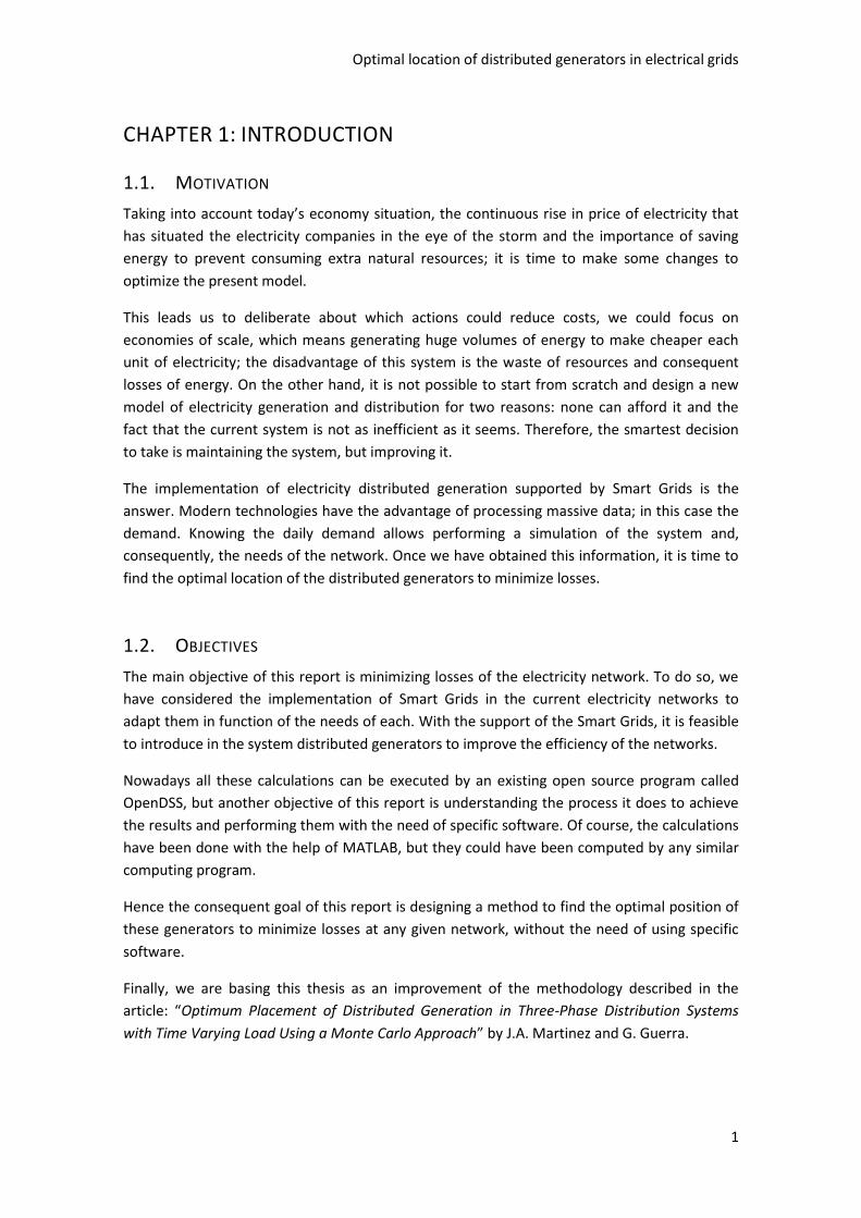
Electric power requires a structure to be able to be transferred from the generation point to
consumers. This structure is the electric distribution grid, each element of this system has a
different function and has different properties. The objective of this chapter is explaining the
basis of the components involved in the electricity distribution.
Figure 1. Sketch of electricity distribution. Source: en.wikipedia.org.
MAIN GENERATION STATION
It is the industrial place where electric power is generated by transforming mechanical power
into electrical power. Most electric power is generated in these important power plants as
they tend to generate high quantities of energy. There is a wide range of energy sources
harnessed to operate the stations; they can use fossil fuels such as natural gas or coal, nuclear
power, hydroelectric power, and so on.
These stations are usually far away from consumer, so we need to transport it. Transformers
are the key piece at this point. They step-up voltage from generators to high-voltage
transmission lines, which are the next element to describe.
TRANSMISSION LINES
They are responsible of the electric power transportation from the generation point to the
customers, either personal or industrial. Due to the need of covering hundreds of kilometers
they are compelled to use high voltage (220 kV or above) three-phase alternating current (AC),
as it is the best way to reduce losses throughout the line.
SUBTRANSMISSION SYSTEM
As soon as we have covered a reasonable distance to reach the consumers, we need to adapt
the electric power to the different demands. It is the task of the substation step down
transformers, which will reduce the power voltage to values between 45 and 132 kV. At this
point power can take two paths: subtransmission customers or primary distribution system. In
CHAPTER 6: CONCLUSIONS
4
the first case, we do not need any other power transformation, as these customers are
adapted to this voltage. We can find factories and some big industries that require this kind of
service.
PRIMARY DISTRIBUTION SYSTEM
In case power continues to the primary distribution system it requires passing through another
transformer to reduce the voltage again, to 11-25 kV. The distance covered is also shorter than
the previous system and like in that case, a share of the market requires this kind of voltages;
for instance small factories.
SECONDARY DISTRIBUTION SYSTEM
The one with the lowest voltage 230-400 V is the obtained after lowering once again the
voltage of the grid. This kind of power will be the demanded mostly for domestic use. This
distribution system is the last step of the distribution system.
2.2. SMART GRIDS
Modernization is fundamental in any service or business because the needs of the consumers
will also evolve, turning our package obsolete; this is why most companies invest in R&D.
Electric power distributors, as a company, should also consider adapting to the current
technologies. Telecommunications have evolved exponentially, which means the capabilities
of information and controlling systems have leeway to grow.
This situation heads us to the implementation of Smart Grids. They are able to use information
and communications technology to gather and act on information, such as information about
the behaviors of consumers and suppliers, in an automated fashion to improve the efficiency,
reliability, economics, and sustainability of the production and distribution of electric power.
2.3. DISTRIBUTED GENERATION
Considering the smart grid has been implemented. We can gather the information of the
entire distribution system and process it. These results will permit the application of
distributed generation with satisfactory outcomes.
Distributed generation is the introduction of small generation centers along the distribution
network near the consumer locations. These generators are directly connected with the
distribution companies and the main objective is to allow collection of energy from many
sources offering several advantages.
Due to the fact that it is based in small generators, this energy can be supplied by small wind
turbines or solar panels, reducing environmental impacts. If we have multiple sources of
energy, the system is not as weak as depending on an only power source, which gives flexibility
in cases of maximum demand. Finally the generation centers are located near the consumer
location, which means that power losses will be reduced.
Optimal location of distributed generators in electrical grids
5
CHAPTER 3: MODEL PROBLEM
3.1. FORMULATION
The objective of this report is finding the optimum placement of distributed generation in
three-phase distribution systems, with losses minimization as target. To do so, it has been
separated in two parts: in first place we will create a method to get losses from any system
and given situation. The second part will be determining methods to choose which of those
situations is the best. In this chapter we are working on the first one, designing a strategy to
calculate losses of any circuit.
3.1.1. MATHEMATICAL MODEL
Before attempting to design a model, we need to consider what kind of model we want to
perform; its limitations, simplifications, hypothesis, etc.
VARIABLES
We have obtained this section’s theory from the book: “Problemas resueltos de sistema de
energía eléctrica, I. J. Ramirez, J. A. Martinez, J. A. Fuentes, E. García, L. A. Fernández, P. J.
Zorzano”.
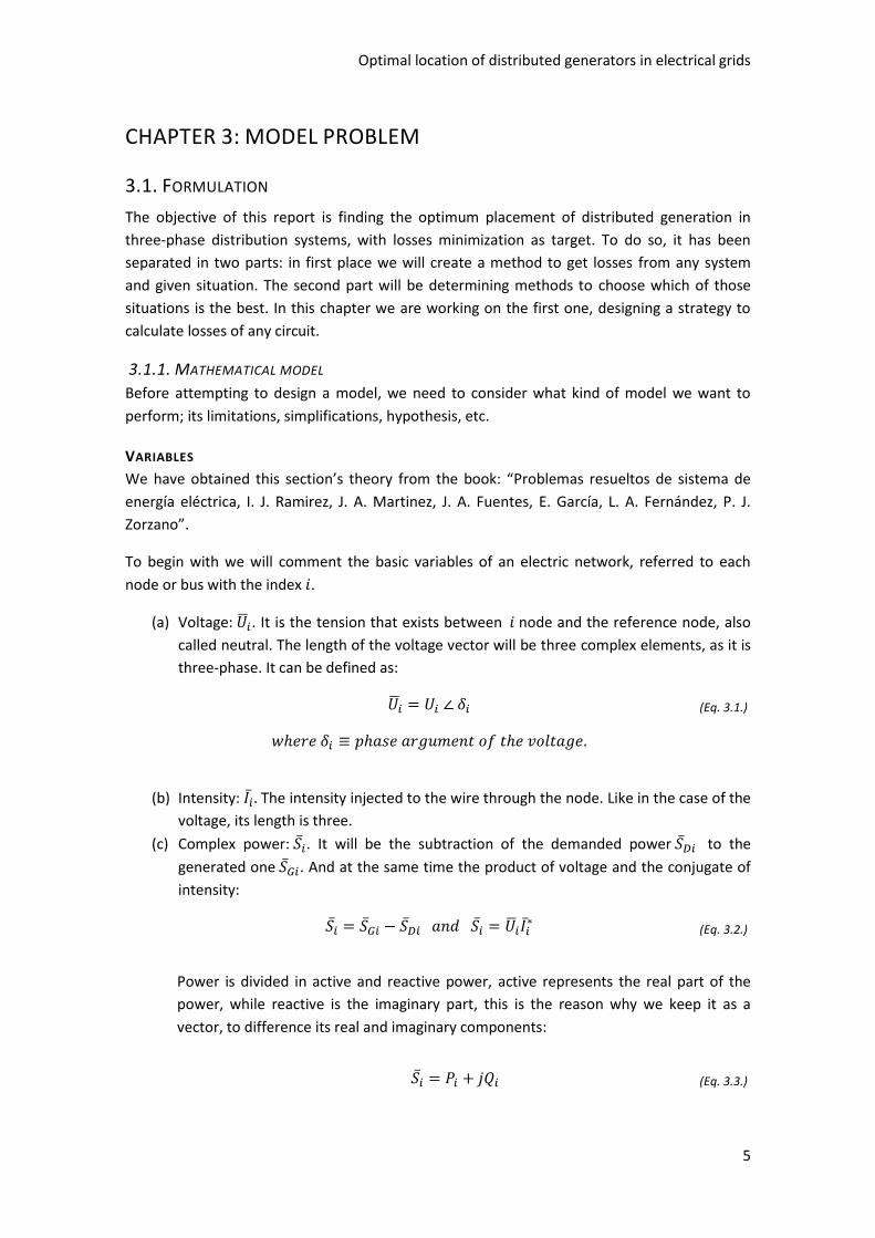
To begin with we will comment the basic variables of an electric network, referred to each
node or bus with the index .
(a) Voltage: . It is the tension that exists between node and the reference node, also
called neutral. The length of the voltage vector will be three complex elements, as it is
three-phase. It can be defined as:
∠ (Eq. 3.1.)
(b) Intensity: The intensity injected to the wire through the node. Like in the case of the
voltage, its length is three.
(c) Complex power: . It will be the subtraction of the demanded power to the
generated one . And at the same time the product of voltage and the conjugate of
intensity:
(Eq. 3.2.)
Power is divided in active and reactive power, active represents the real part of the
power, while reactive is the imaginary part, this is the reason why we keep it as a
vector, to difference its real and imaginary components:
(Eq. 3.3.)
CHAPTER 6: CONCLUSIONS
6
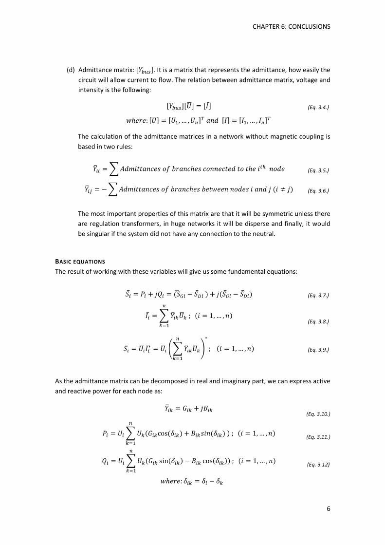
(d) Admittance matrix: [ ]. It is a matrix that represents the admittance, how easily the
circuit will allow current to flow. The relation between admittance matrix, voltage and
intensity is the following:
[ ][ ] [ ] (Eq. 3.4.)
[ ] [ ] [ ] [ ]
The calculation of the admittance matrices in a network without magnetic coupling is
based in two rules:
∑ (Eq. 3.5.)
∑ (Eq. 3.6.)
The most important properties of this matrix are that it will be symmetric unless there
are regulation transformers, in huge networks it will be disperse and finally, it would
be singular if the system did not have any connection to the neutral.
BASIC EQUATIONS
The result of working with these variables will give us some fundamental equations:
(Eq. 3.7.)
∑
(Eq. 3.8.)
(∑
)
(Eq. 3.9.)
As the admittance matrix can be decomposed in real and imaginary part, we can express active
and reactive power for each node as:
(Eq. 3.10.)
∑
(Eq. 3.11.)
∑
(Eq. 3.12)
CHAPTER 6: CONCLUSIONS
7
HYPOTHESIS
1. THREE-PHASE ALTERNATE SYSTEM
As it is commented in previous chapters, electrical grids are based in a three-phase system,
because it is the most economical, compared with single or two-phase systems at the
same voltage; so each node will have three complex voltages.
2. PQ GENERATION NODES
Each of the generation nodes will be called PQ nodes. This means that in case there is no
generation a particular node, we can know the active and reactive power of it. Leaving as
variables the voltage and .
3. TIME VARYING APPLIED LOADS
The objective is performing a losses year simulation. We will work with two different
modes; the first one will be the analysis of constant demand snapshots (snapshot mode).
The second one will consider load curves in each node along the year (time mode) and
another load curve in the implemented distributed generator.
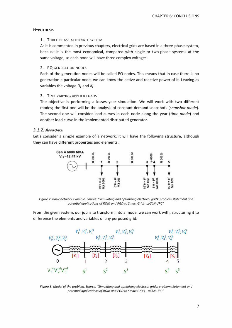
3.1.2. APPROACH
Let’s consider a simple example of a network; it will have the following structure, although
they can have different properties and elements:
Figure 2. Basic network example. Source: “Simulating and optimizing electrical grids: problem statement and potential applications of ROM and PGD to Smart Grids, LaCàN UPC”.
From the given system, our job is to transform into a model we can work with, structuring it to
difference the elements and variables of any purposed grid:
Figure 3. Model of the problem. Source: “Simulating and optimizing electrical grids: problem statement and potential applications of ROM and PGD to Smart Grids, LaCàN UPC”.
CHAPTER 6: CONCLUSIONS
8
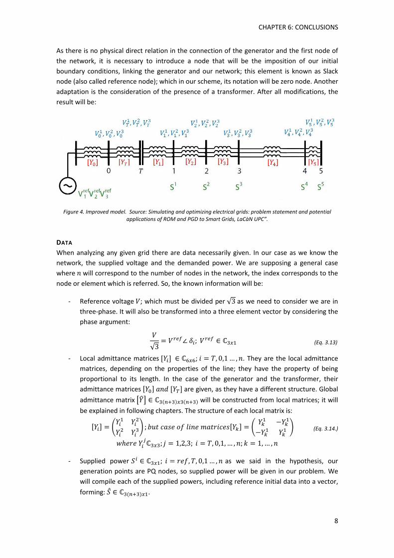
As there is no physical direct relation in the connection of the generator and the first node of
the network, it is necessary to introduce a node that will be the imposition of our initial
boundary conditions, linking the generator and our network; this element is known as Slack
node (also called reference node); which in our scheme, its notation will be zero node. Another
adaptation is the consideration of the presence of a transformer. After all modifications, the
result will be:
Figure 4. Improved model. Source: Simulating and optimizing electrical grids: problem statement and potential applications of ROM and PGD to Smart Grids, LaCàN UPC”.
DATA
When analyzing any given grid there are data necessarily given. In our case as we know the
network, the supplied voltage and the demanded power. We are supposing a general case
where will correspond to the number of nodes in the network, the index corresponds to the
node or element which is referred. So, the known information will be:
- Reference voltage ; which must be divided per √ as we need to consider we are in
three-phase. It will also be transformed into a three element vector by considering the
phase argument:
√ ∠
(Eq. 3.13)
- Local admittance matrices [ ] ; . They are the local admittance
matrices, depending on the properties of the line; they have the property of being
proportional to its length. In the case of the generator and the transformer, their
admittance matrices [ ] [ ] are given, as they have a different structure. Global
admittance matrix [ ] will be constructed from local matrices; it will
be explained in following chapters. The structure of each local matrix is:
[ ] (
) [ ] (
) (Eq. 3.14.)
- Supplied power as we said in the hypothesis, our
generation points are PQ nodes, so supplied power will be given in our problem. We
will compile each of the supplied powers, including reference initial data into a vector,
forming: .
CHAPTER 6: CONCLUSIONS
9
It is important to take into account that these data are complex, so we would have the double
quantity of data in the calculations if we transformed it into real numbers.
UNKNOWNS
If we had not unknowns there would not be problem to solve, so the initial unknowns to
calculate are the voltages of each node:
- Bus voltages . Which will form the unknown vector:
[
] .
3.1.3. EQUATIONS AND RESOLUTION
The governing equation which rules the problem is:
(∑
)
(∑
) (Eq. 3.15.)
[
]
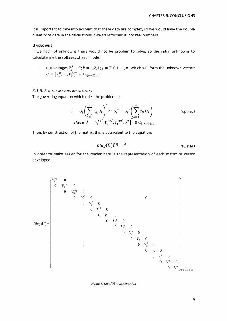
Then, by construction of the matrix, this is equivalent to the equation:
( ) (Eq. 3.16.)
In order to make easier for the reader here is the representation of each matrix or vector
developed:
)3(3)3(33
2
1
1
3
1
2
1
1
3
2
1
0
3
0
2
0
1
3
2
1
0
00
00
00
000
00
00
00
00
00
00
00
000
00
00
0
)ˆ(
nxn
n
n
n
T
T
T
ref
ref
ref
V
V
V
V
V
V
V
V
V
V
V
V
V
V
V
UDiag
Figure 5. Diag(Û) representation
CHAPTER 6: CONCLUSIONS
10
)3(3)3(3
12
111
1
1
2
1
1
1
1
1
1
1
1
32
211
0
1
0
1
0
1
0
ˆ
nxnnn
nnn
TT
TT
YY
YYY
YYY
YYYY
YYYY
YY
Y
Figure 6. Global admittance matrix representation
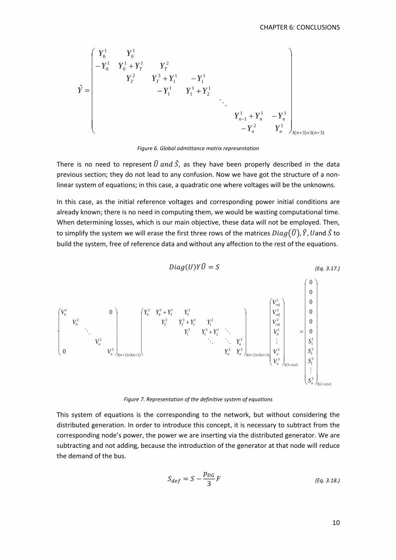
There is no need to represent , as they have been properly described in the data
previous section; they do not lead to any confusion. Now we have got the structure of a non-
linear system of equations; in this case, a quadratic one where voltages will be the unknowns.
In this case, as the initial reference voltages and corresponding power initial conditions are
already known; there is no need in computing them, we would be wasting computational time.
When determining losses, which is our main objective, these data will not be employed. Then,
to simplify the system we will erase the first three rows of the matrices ( ) and to
build the system, free of reference data and without any affection to the rest of the equations.
(Eq. 3.17.)
1)2(3
3
3
1
2
1
1
1
1)3(3
3
2
1
0
3
2
1
)3(3)2(3
32
2
1
2
3
1
2
1
2
1
1
1
32
213
0
2
0
)2(3)2(3
3
2
2
0
1
0
0
0
0
0
0
0
0
0
·
xnn
xnn
n
ref
ref
ref
nxnnn
n
TT
TT
nxnn
n
S
S
S
S
V
V
V
V
V
V
YY
Y
YYY
YYYY
YYYY
V
V
V
V
Figure 7. Representation of the definitive system of equations
This system of equations is the corresponding to the network, but without considering the
distributed generation. In order to introduce this concept, it is necessary to subtract from the
corresponding node’s power, the power we are inserting via the distributed generator. We are
subtracting and not adding, because the introduction of the generator at that node will reduce
the demand of the bus.
(Eq. 3.18.)
CHAPTER 6: CONCLUSIONS
11
{
(Eq. 3.19.)
As it is a non-linear system of equations, the best idea is to solve the system using the Newton
Raphson method. Its basic structure to solve systems of equations is the following:
Newton-Raphson structure:
( )
{
}
(
)
(Eq. 3.20.)
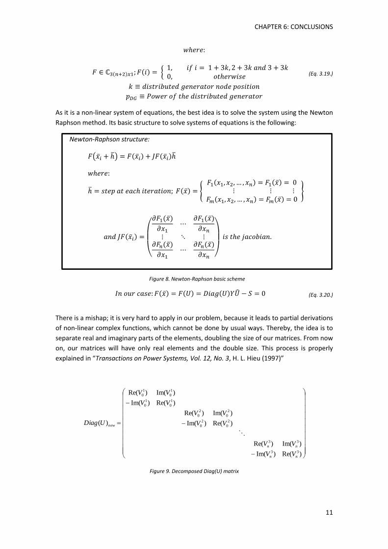
There is a mishap; it is very hard to apply in our problem, because it leads to partial derivations
of non-linear complex functions, which cannot be done by usual ways. Thereby, the idea is to
separate real and imaginary parts of the elements, doubling the size of our matrices. From now
on, our matrices will have only real elements and the double size. This process is properly
explained in “Transactions on Power Systems, Vol. 12, No. 3, H. L. Hieu (1997)”
)Re()Im(
)Im()Re(
)Re()Im(
)Im()Re(
)Re()Im(
)Im()Re(
)(
33
33
2
0
2
0
2
0
2
0
1
0
1
0
1
0
1
0
nn
nn
new
VV
VV
VV
VV
VV
VV
UDiag
Figure 9. Decomposed Diag(U) matrix
Figure 8. Newton-Raphson basic scheme
CHAPTER 6: CONCLUSIONS
12
)Re()Im(
)Im()Re(
)Re()Im()Re()Im(
)Im()Re()Im()Re(
)Re()Im()Re()Im()Re()Im(
)Im()Re()Im()Re()Im()Re(
11
11
1
1
31
1
322
1
1
31
1
322
2211
0
11
0
1
0
1
0
2211
0
11
0
1
0
1
0
nn
nn
TTTT
TTTT
TTTT
TTTT
new
YY
YY
YYYYYY
YYYYYY
YYYYYYYY
YYYYYYYY
Y
Figure 10. Decomposed modified global admittance matrix
)Im(
)Re(
)Im(
)Re(
)Im(
)Re(
0
0
;
)Im(
)Re(
)Im(
)Re(
)Im(
)Re(
3
3
2
2
1
1
1
1
1
3
3
2
2
0
1
0
1
0
n
n
n
new
n
n
n
new
S
S
S
S
S
S
S
V
V
V
V
V
V
U
Figure 11. Decomposed voltage and power vectors
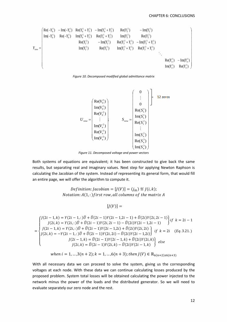
Both systems of equations are equivalent; it has been constructed to give back the same
results, but separating real and imaginary values. Next step for applying Newton Raphson is
calculating the Jacobian of the system. Instead of representing its general form, that would fill
an entire page, we will offer the algorithm to compute it.
[ ]
[ ]
{
}
}
}
With all necessary data we can proceed to solve the system, giving us the corresponding
voltages at each node. With these data we can continue calculating losses produced by the
proposed problem. System total losses will be obtained calculating the power injected to the
network minus the power of the loads and the distributed generator. So we will need to
evaluate separately our zero node and the rest.
CHAPTER 6: CONCLUSIONS
13
First step is calculating the intensity of our slack bus. To calculate it, we must take into account
the influence of the transformer. So it is necessary to look at the admittance matrix and
choose the proper elements:
(
) (
) (Eq. 3.22.)
(
) (Eq. 3.23.)
As we have calculated all the unknowns of the system in the previous step; we can apply the
Equation 3.16 to obtain the loads at each of the nodes. From the new computed vector we
will take all the elements from the seventh position, as we are only interested in the real nodes
loads. These elements are individual data, but we are looking forward the total situation; we
will sum all the elements to find the global result:
∑
∑
(Eq. 3.24.)
Last step is adding one to another and taking only the real part of the sum:
(Eq. 3.25.)
We are adding and not subtracting like we said previously, because the demanded power is
already negative by concept. This is why in the explanation we mentioned it was needed to do
a subtraction and in the formulation we are doing a sum.
3.1.4. POWER FLOW
Demanded power is our independent element in the equations we have explained, but we
have not talked about how we choose this parameter. There are two ways of considering the
power flow. On one hand we have got the snapshot mode, whilst on the other hand there is
the time mode.
SNAPSHOT MODE
This is the simplest case we can consider, we are supposing a constant power demand during
an instantaneous lapse of time; the idea is taking a photo of the system demand and stored as
our , this is why it is called snapshot.
In order to compute losses with this mode, it will be necessary to solve the previous system of
equations only once; this leads to an advantage of this mode: its speed. On the other hand, the
CHAPTER 6: CONCLUSIONS
14
con of this mode is that we are not evaluating a varying load; we are only obtaining an instant
evaluation of the system. It could be used, for instance, to calculate a punctual maximum
demand situation.
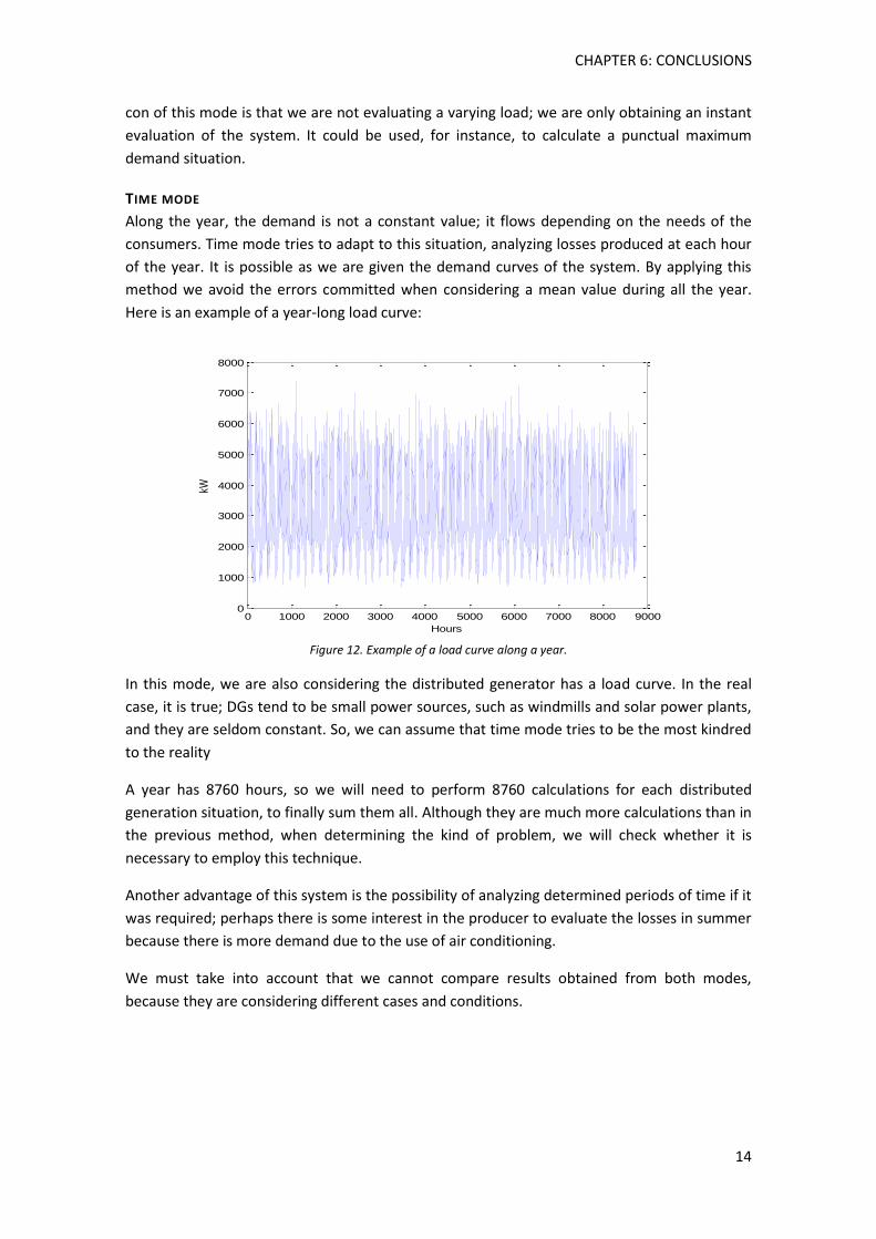
TIME MODE
Along the year, the demand is not a constant value; it flows depending on the needs of the
consumers. Time mode tries to adapt to this situation, analyzing losses produced at each hour
of the year. It is possible as we are given the demand curves of the system. By applying this
method we avoid the errors committed when considering a mean value during all the year.
Here is an example of a year-long load curve:
Figure 12. Example of a load curve along a year.
In this mode, we are also considering the distributed generator has a load curve. In the real
case, it is true; DGs tend to be small power sources, such as windmills and solar power plants,
and they are seldom constant. So, we can assume that time mode tries to be the most kindred
to the reality
A year has 8760 hours, so we will need to perform 8760 calculations for each distributed
generation situation, to finally sum them all. Although they are much more calculations than in
the previous method, when determining the kind of problem, we will check whether it is
necessary to employ this technique.
Another advantage of this system is the possibility of analyzing determined periods of time if it
was required; perhaps there is some interest in the producer to evaluate the losses in summer
because there is more demand due to the use of air conditioning.
We must take into account that we cannot compare results obtained from both modes,
because they are considering different cases and conditions.
0 1000 2000 3000 4000 5000 6000 7000 8000 90000
1000
2000
3000
4000
5000
6000
7000
8000
Hours
kW
CHAPTER 6: CONCLUSIONS
15
3.2. OPENDSS
The Open Distribution System Simulator, OpenDSS, is a comprehensive electrical system
simulation software for electric utility distribution systems. It has been under development by
EPRI (Electric Power Research Institute) for more than 15 years. It can support nearly all
frequency domain (sinusoidal steady‐state) analyses commonly performed on electric utility
power distribution systems. Moreover, the idea of being open source and continuously
updating, supports several new types of analyses, which are designed to meet future needs
related to smart grid, grid modernization and renewable energy research.
It is implemented as both a standalone executable program (.EXE) and as a dynamic link library
(.DLL) designed as an in-process server to be driven form a wide range of existing calculation
software platforms.
On one hand, the EXE version provides a multiple-window user interface to assist users in
constructing and executing scripts. It basically supports all RMS steady state analyses
commonly performed on electric power distribution systems, such as power flow, fault current
calculations and harmonic analysis. In addition, it supports many new types of analyses that
are designed to meet future needs, many of which are being dictated by the deregulation of
US utilities and the formation of distribution companies worldwide.
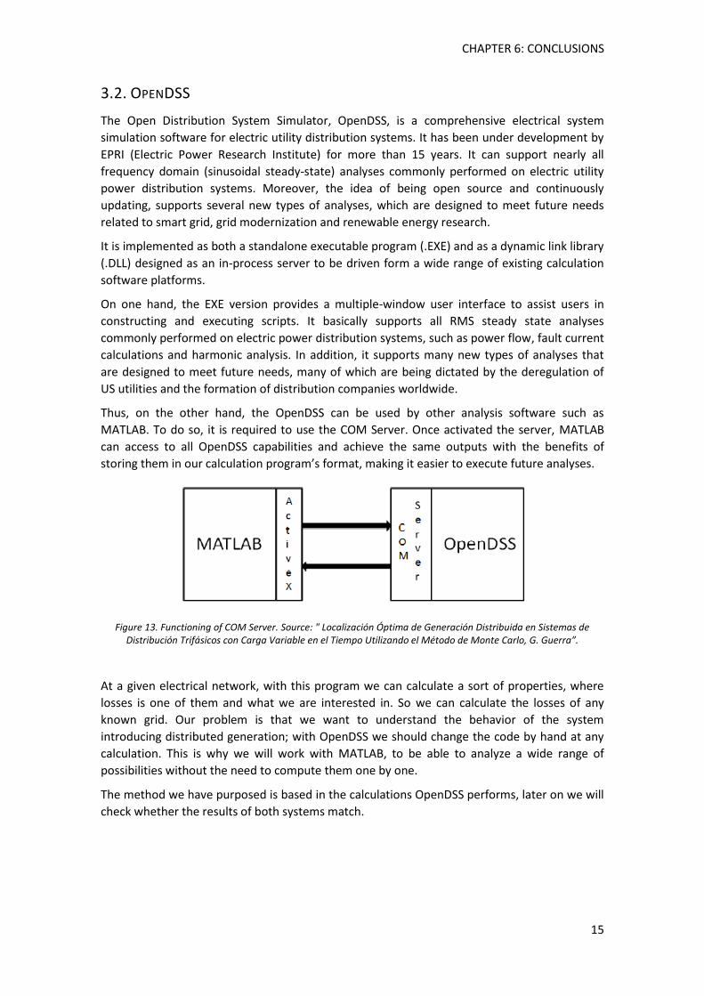
Thus, on the other hand, the OpenDSS can be used by other analysis software such as
MATLAB. To do so, it is required to use the COM Server. Once activated the server, MATLAB
can access to all OpenDSS capabilities and achieve the same outputs with the benefits of
storing them in our calculation program’s format, making it easier to execute future analyses.
Figure 13. Functioning of COM Server. Source: " Localización Óptima de Generación Distribuida en Sistemas de Distribución Trifásicos con Carga Variable en el Tiempo Utilizando el Método de Monte Carlo, G. Guerra”.
At a given electrical network, with this program we can calculate a sort of properties, where
losses is one of them and what we are interested in. So we can calculate the losses of any
known grid. Our problem is that we want to understand the behavior of the system
introducing distributed generation; with OpenDSS we should change the code by hand at any
calculation. This is why we will work with MATLAB, to be able to analyze a wide range of
possibilities without the need to compute them one by one.
The method we have purposed is based in the calculations OpenDSS performs, later on we will
check whether the results of both systems match.
Optimal location of distributed generators in electrical grids
16
CHAPTER 4: OPTIMIZATION
4.1. INTRODUCTION
An optimization problem consists of maximizing or minimizing a real function by systematically
choosing input values from within an allowed set and computing the value of the function,
until we reach the desired result. More generally, optimization includes finding best available
values of some objective function given a defined domain. The general problem will be:
(Eq. 4.1.)
Where is the objective function to be minimized over the variable ; are the
inequality constraints and are the equality constraints. As we see the general case is
defined, by convention, as a minimization problem. In case we wanted to turn it into a
maximization one, negating the objective function is enough to obtain the maximum.
There are several methods to choose when optimizing, they will depend on the objective
functions or the kind of variables and constraints. We can separate three main groups of
optimization methods, although they could be combined to improve the efficiency of the
calculations:
DIRECT METHODS
They attempt to solve the problem by a finite sequence of operations. This sequence of
equations is a determined algorithm that will be restricted to a number. They are solid for
linear programming, but apart from that they are not used. Simplex algorithm or its variants is
the most employed technique in this group.
ITERATIVE METHOD
This technique is based in the generation of a sequence of improving approximate solutions for
a certain type of problem. Each iteration is intended to be closer to the objective than the
previous one. Put differently, each step tries to converge to the minimum or maximum value
of the function in our domain. They are usually employed in non-linear problems and the
method used depends on the information and requirements of the problem; using only
evaluations of the function like Pattern Search methods, gradients of the function such as
Quasi-Newton or Gradient Descend methods or lastly Newton methods, which evaluate the
Hessian of the function. The criterion to finish the iterations depends on the users and the
accuracy they want to achieve. Higher accuracies imply higher computational costs.
In most cases functions are not quadratic, so these methods might fall in a local minimum and
get stuck in this point. To avoid this situation and ensure global convergence the use of a line
search or a trust region combined with the method is highly recommendable.
CHAPTER 6: CONCLUSIONS
17
HEURISTIC METHODS
Heuristic methods are based in trial and error for solving problems. These methods are not
guaranteed to be optimal, but they work well and offer us global convergence when being
executed properly. They also perform iterations to solve the problem, but they do not need to
converge at each of them. In the report we will employ Genetic Algorithms, which belong to
this kind of solvers.
STOCHASTIC METHODS
They are optimization methods that are based in the generation of random variables;
therefore it becomes a probability method. The higher evaluations of the objective function,
the higher probability to obtain the minima or maxima. An example of this method is Monte
Carlo approach.
4.2. OBJECTIVE
Whichever optimization method we are using, the objective in essence is the same: looking for
the minimum. In our problem, the objective to minimize is the grid power losses.
The objective and structure of this project is based in the article “Optimum Placement of
Distributed Generation in Three-Phase Distribution Systems with Time Varying Load Using a
Monte Carlo Approach” written by Juan A. Martinez and Gerardo Guerra, where they try to
solve this problem applying Monte Carlo approach.
It is a good idea to do this calculations with this method, as it is comfortable to perform, but
the problem is that we are randomly sampling inside all the domain, which means that we are
analyzing points that do not contribute to the problem solving; this method is supported on big
samples of possible results. The bigger samples we have, the higher probability to find the
minimum in our sample. To ensure its effectiveness it is necessary to perform hundreds or
thousands of computations.
Considering each calculation requires a considerable time, we should contemplate using other
techniques, which do not depend only in luck. This is the reason why in the next sections we
are analyzing Genetic Algorithms and Broyden Fletcher Goldfarb Shanno; two different
optimization methods.
4.3. GENETIC ALGORITHMS
Genetic algorithms (GA from now on) is an optimization heuristic method that evolves the
answer until it reaches an acceptable result. It uses a routine similar to the natural selection
process to achieve the global solution of the problem.
In nature, animals of a habitat compete with each other to get to the resources of the area and
survive. Inside their own species, they also need to confront each other in order to find a
member of the other gender to reproduce and continue the lineage. Those specimens, who
have higher rate of survival, also have higher chances of having offspring; at the same time,
the ones with lower rate of survival will have a lower amount of descendants. This means that
CHAPTER 6: CONCLUSIONS
18
better adapted specimens will propagate their pedigree in future generations. As Darwin
defends, only the best ones will survive, having in the future the best combination of genes
from that specie. In nature there can also be mutations, some members of the specie can be
born with a mutated characteristic that might help him surviving or making him weaker, only
in the first case this mutation will be maintained in future specimen.
This little entry is necessary to understand why the name of this method is genetic algorithms.
First of all we have got the initial population; each of the members is a feasible solution of the
problem. Analyzing them, it is possible to evaluate their quality comparing them to the
solution desired. Discarding the worst ones, we will generate a new part of the population
crossing data from the surviving elements, introducing some mutations. Now the process is the
same: evaluating them, discarding and generating until we reach the global minimum: the
perfect specie. So now this report will explain in detail each of the steps of this process.
4.2.1. PROCESS
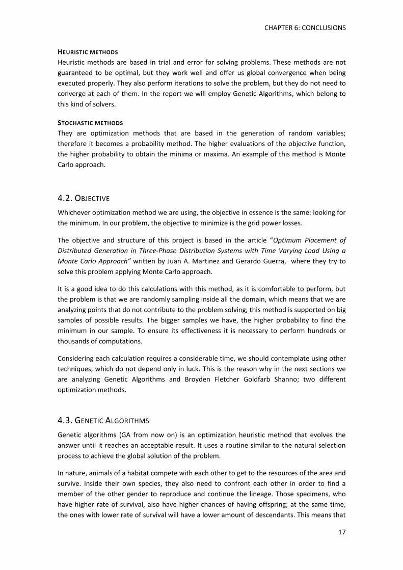
ENCODING
Before a genetic algorithm can be put to work on any problem, it is needed to encode
potential solutions. They are stored in strings that will content the information of the
solutions. Each solution will be represented by one of these strings and it will be called
chromosome.
Chromosome: 0 1 0 1 0 0 1
Gene: 0
Each chromosome will be formed by genes, which are the parameters of the solution. Genes
will be stored in binary code. Although it looks more complicated than decimal coding, for
further steps of the algorithm it becomes an advantage. With an example it becomes easier to
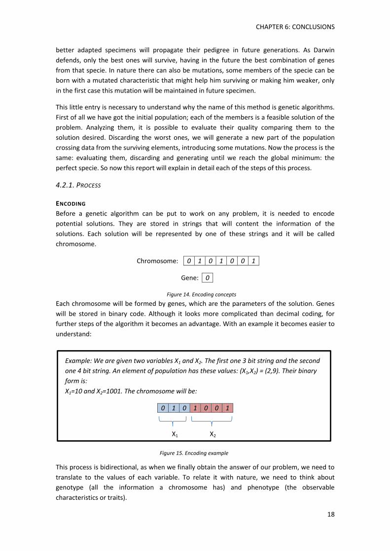
understand:
Example: We are given two variables X1 and X2. The first one 3 bit string and the second
one 4 bit string. An element of population has these values: (X1,X2) = (2,9). Their binary
form is:
X1=10 and X2=1001. The chromosome will be:
0 1 0 1 0 0 1
X1 X2
This process is bidirectional, as when we finally obtain the answer of our problem, we need to
translate to the values of each variable. To relate it with nature, we need to think about
genotype (all the information a chromosome has) and phenotype (the observable
characteristics or traits).
Figure 14. Encoding concepts
Figure 15. Encoding example
CHAPTER 6: CONCLUSIONS
19
INITIAL POPULATION
The original population must be created randomly, attending to the conditions and constraints
of the problem. In this point we can either define which kind of variables we are accepting; for
instance one of the variables could be forced to be integer and negative; it will depend on the
problem.
Size of population is another consideration that should be taken into account, because the size
of our sample will condition the study. In case we had too few elements, there sample would
not be representing the reality; whereas if it had too many, the computational cost would be
too high including redundant information.
SELECTION
Once we’ve got the initial population, it is time to work with it; otherwise it would be a Monte
Carlo method. Next stage is evaluating the population, that according to Darwin’s evolution
theory, only the fittest survive. The way of quantifying the optimality of a solution is through
the fitness function. This function depicts the closeness of an existing solution to the desired
result. Depending on the affinity to the desired solution, each of the chromosomes is given a
score. Higher scores imply higher fitness and lower the opposite. Now it is possible to proceed
with the selection.
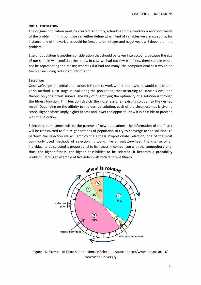
Selected chromosomes will be the parents of new populations; the information of the fittest
will be transmitted to future generations of population to try to converge to the solution. To
perform the selection we will employ the Fitness Proportionate Selection, one of the most
commonly used methods of selection. It works like a roulette-wheel: the chance of an
individual to be selected is proportional to its fitness in comparison with the competitors’ one;
thus, the higher fitness, the higher possibilities to be selected. It becomes a probability
problem. Here is an example of five individuals with different fitness.
Figure 16. Example of Fitness Proportionate Selection. Source: http://www.edc.ncl.ac.uk/,
Newcastle University
CHAPTER 6: CONCLUSIONS
20
There are some probabilistic methods that instead of considering a proportional relation
between fitness and probability of survival, they work with exponentials. Some methods
automatically discard the lowest fit, maintain the medium ones and duplicate the fittest ones.
We have employed the Roulette because it is easier to understand.
OFFSPRING
Surviving individuals after the selection have become the parents of future populations as they
have the best information at the moment. The offspring will be the result of combining the
chromosomes of two different parents to create new ones. This process is called crossover.
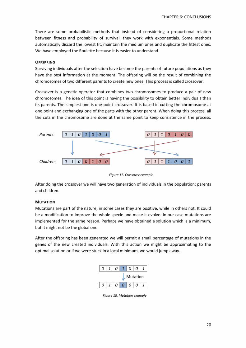
Crossover is a genetic operator that combines two chromosomes to produce a pair of new
chromosomes. The idea of this point is having the possibility to obtain better individuals than
its parents. The simplest one is one-point crossover. It is based in cutting the chromosome at
one point and exchanging one of the parts with the other parent. When doing this process, all
the cuts in the chromosome are done at the same point to keep consistence in the process.
Parents: 0 1 0 1 0 0 1 0 1 1 0 1 0 0
Children: 0 1 0 0 1 0 0 0 1 1 1 0 0 1
After doing the crossover we will have two generation of individuals in the population: parents
and children.
MUTATION
Mutations are part of the nature, in some cases they are positive, while in others not. It could
be a modification to improve the whole specie and make it evolve. In our case mutations are
implemented for the same reason. Perhaps we have obtained a solution which is a minimum,
but it might not be the global one.
After the offspring has been generated we will permit a small percentage of mutations in the
genes of the new created individuals. With this action we might be approximating to the
optimal solution or if we were stuck in a local minimum, we would jump away.
0 1 0 1 0 0 1
0 1 0 0 0 0 1
Mutation
Figure 17. Crossover example
Figure 18. Mutation example
CHAPTER 6: CONCLUSIONS
21
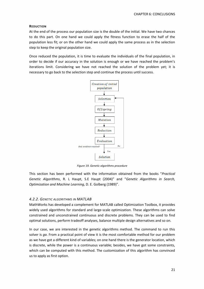
REDUCTION
At the end of the process our population size is the double of the initial. We have two chances
to do this part. On one hand we could apply the fitness function to erase the half of the
population less fit; or on the other hand we could apply the same process as in the selection
step to keep the original population size.
Once reduced the population, it is time to evaluate the individuals of the final population, in
order to decide if our accuracy in the solution is enough or we have reached the problem’s
iterations limit. Considering we have not reached the solution of the problem yet; it is
necessary to go back to the selection step and continue the process until success.
Figure 19. Genetic algorithms procedure
This section has been performed with the information obtained from the books “Practical
Genetic Algorithms, R. L Haupt, S.E Haupt (2004)” and “Genetic Algorithms in Search,
Optimization and Machine Learning, D. E. Golberg (1989)".
4.2.2. GENETIC ALGORITHMS IN MATLAB
MathWorks has developed a complement for MATLAB called Optimization Toolbox, it provides
widely used algorithms for standard and large-scale optimization. These algorithms can solve
constrained and unconstrained continuous and discrete problems. They can be used to find
optimal solutions, perform tradeoff analyses, balance multiple design alternatives and so on.
In our case, we are interested in the genetic algorithms method. The command to run this
solver is ga. From a practical point of view it is the most comfortable method for our problem
as we have got a different kind of variables; on one hand there is the generator location, which
is discrete, while the power is a continuous variable; besides, we have got some constraints,
which can be computed with this method. The customization of this algorithm has convinced
us to apply as first option.

CHAPTER 6: CONCLUSIONS
22
Firstly it is necessary to determine our objective function. It is the script we created to evaluate
the losses given the generator position and the power supplied, turned into a function and
leaving them as variables. Then, next step is confirming that our function depends on two
variables.
Now is time to impose constraints; they are introduced as lower and upper bound. As we have
two variables, it will be understood as a rectangle where population must be inside it. The
lower bound will be the minimum value permitted of each variable: first node and absence of
power supply; the upper bound will be the maximum values: last node and the maximum
power accepted by the system, to ensure our script does not accumulate errors in calculations.
The remaining constraint will be the limitation of the position variable, imposing it to be an
integer number.
To make the solver efficient, it is important to choose some parameters of the program. Let’s
introduce the basic introduced functions, first of all population. Population can be of different
types depending on the problem, if we had a binary problem optimization we would use Bit
string, but as we are working with a mixed integer programming, we will choose the double
vector option. It is also possible to introduce an initial population, but in our case we start from
scratch, so we let Maltab to create it randomly. When choosing its size we will apply the
default option which employs the following formula:
(Eq. 4.2.)
When choosing fitness, we can decide between different methods, but our decision is to take
the Roulette-wheel method; as it is the one we commented in the previous chapter and the
results are expected to be fine.
To configure offspring, firstly we need to specify the minimum number of individuals that are
guaranteed to survive to the next generation; in case of integer problems, the default option
will be:
(Eq. 4.3.)
We will consider it good enough, next step is determining the crossover fraction. A crossover
fraction of 1 means that all children other than elite individuals are crossover children; while a
crossover fraction of 0 means that all children are mutated children. About these mutations,
Maltab suggests not using in integer programming, but as one of the variables is not integer,
we accept them; therefore the value of crossover fraction will be lower than one. Finally the
kind of crossover will be a single point one, as we have got only 2 variables. There is no need of
changing the default options.
Genetic algorithm performs iterations to reach the solution, so it is necessary to determine a
stopping criterion. Most popular criterion is accuracy; once we reach a reasonable fitness
value, we stop the iterations and take the result as definitive. In order to avoid divergence of
the functions it is also recommended to introduce a maximum number of generations,
avoiding an infinite buckle of iterations.
CHAPTER 6: CONCLUSIONS
23
4.3. BROYDEN FLETCHER GOLDFARB SHANNO
4.3.1. INTRODUCTION
For this section, we have obtained the formulation from “”The solution of non linear finite
element equations, H. Matthies; G. Strang (1979)” and “Updating Quasi-Newton Matrices with
Limited Storage, J. Nocedal (1980)”
BFGS is a Quasi-Newton method for solving unconstrained non-linear optimization problems.
In Newton’s method, it is used a second order Taylor approximation to find the minimum of a
function:
(Eq. 4.4.)
Where it is needed the gradient and the Hessian of the function we are optimizing. This
Hessian is sometimes difficult to find. This is why Quasi-Newton Methods exist; they perform
an approximation of the Hessian. The Hessian is computed by analyzing successive gradient
vectors.
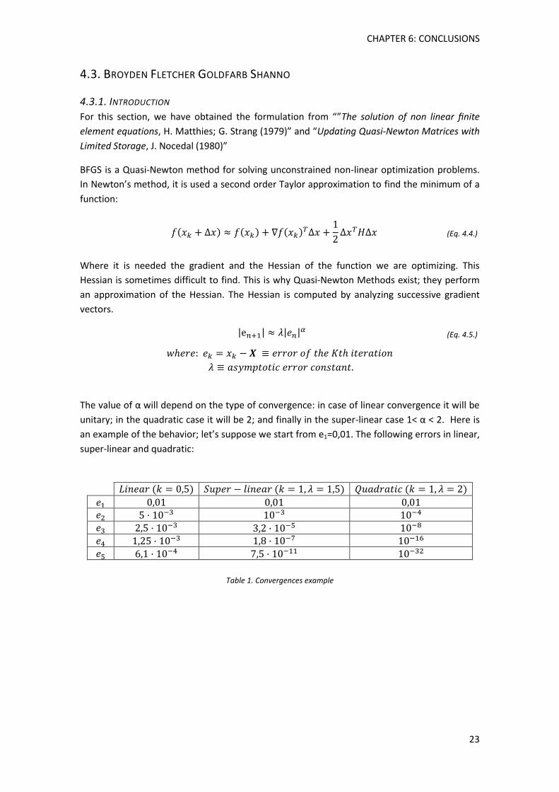
| | | | (Eq. 4.5.)
The value of α will depend on the type of convergence: in case of linear convergence it will be
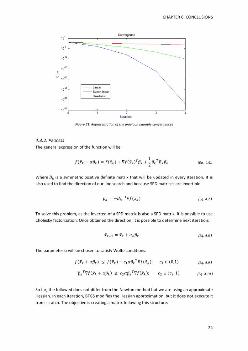
unitary; in the quadratic case it will be 2; and finally in the super-linear case 1< α < 2. Here is
an example of the behavior; let’s suppose we start from e1=0,01. The following errors in linear,
super-linear and quadratic:
Table 1. Convergences example
CHAPTER 6: CONCLUSIONS
24
Figure 21. Representation of the previous example convergences
4.3.2. PROCESS
The general expression of the function will be:
(Eq. 4.6.)
Where is a symmetric positive definite matrix that will be updated in every iteration. It is
also used to find the direction of our line search and because SPD matrices are invertible:
(Eq. 4.7.)
To solve this problem, as the inverted of a SPD matrix is also a SPD matrix, it is possible to use
Cholesky factorization. Once obtained the direction, it is possible to determine next iteration:
(Eq. 4.8.)
The parameter α will be chosen to satisfy Wolfe conditions:
(Eq. 4.9.)
(Eq. 4.10.)
So far, the followed does not differ from the Newton method but we are using an approximate
Hessian. In each iteration, BFGS modifies the Hessian approximation, but it does not execute it
from scratch. The objective is creating a matrix following this structure:
CHAPTER 6: CONCLUSIONS
25
(Eq. 4.11.)
At the same time it is necessary to satisfy the next condition:
(Eq. 4.12.)
(Eq. 4.13.)
To make it more comfortable we change the notation, remaining:
(Eq. 4.14.)
(Eq. 4.15.)
(Eq. 4.16.)
To verify the curvature condition we need to multiply both sides of the equality per
(Eq. 4.17.)
Imposing again Wolfe conditions on the line search procedure, the curvature condition will
always hold:
(Eq. 4.18.)
(Eq. 4.19.)
We can affirm this statement as attending to Wolfe conditions and is a descending
direction. Therefore, always that curvature condition is satisfied, the secant equation will have
at least one feasible . The idea of BFGS is imposing conditions to the inverse of and the
secant equation will be equivalent to:
(Eq. 4.20.)
As there is the possibility of having several matrixes which verify the secant equation; we
will have to perform a matrix minimization problem and choose only one of the solutions. The
chosen matrix will be the closest to
‖ ‖ (Eq. 4.21.)
The definition of this norm will condition the kind of Quasi-Newton method we are facing. In
case of BFGS we will employ weighted Frobenius norm.
CHAPTER 6: CONCLUSIONS
26
‖ ‖ √∑∑| |
√ ∑
(Eq. 4.22.)
The result of solving this minimization gives us the definitive for our problem.
( ) (
)
(Eq. 4.23.)
To get the expression back in function of and , we will use the Sherman Morrison
theorem; which is a particular case of the Woodbury matrix identity.
(Eq. 4.24.)
Applied to the previous expression of will give us:
(Eq. 4.25.)
Obtaining the value from the Equation 4.9 and, consequently, a system to obtain the
Hessian approximation which evolves using most recent data, combined with existing
knowledge in the previous steps.
Finally it is necessary to define how the first approximation of the Hessian will be defined. The
best way will be performing a finite difference approximation at the initial point, as it will
behave locally like the real one.
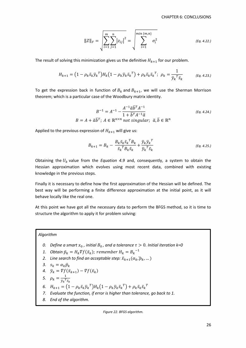
At this point we have got all the necessary data to perform the BFGS method, so it is time to
structure the algorithm to apply it for problem solving:
Algorithm
0. Define a smart , initial , and a tolerance . Initial iteration k=0
1. Obtain
2. Line search to find an acceptable step:
3.
4.
5.
6. ( ) (
)
7. Evaluate the function, if error is higher than tolerance, go back to 1.
8. End of the algorithm.
Figure 22. BFGS algorithm.
CHAPTER 6: CONCLUSIONS
27
To sum up, BFGS update is a good rank-two update, which satisfies the secant equation and
preserves symmetry and positive definiteness of the matrix. Its convergence is super-linear
and it is not required to know or compute the Hessian of our objective function; which gives
out an appropriate relation between computational cost and performance.
4.3.3. BFGS IN MATLAB
In MATLAB’s optimization toolbox we have the possibility of applying BFGS method. The
command to run this solver is fminunc. It finds the minimum of an unconstrained problem. Like
in genetic algorithm’s case, our variables will be the position of the distributed generator and
the power applied to it.
It is true that our problem is a constrained one, but the fact is that when having only one
distributed generator, losses tend to descend towards a central point. It could be also thought
as logical, the furthest from most points the generator is, the higher losses we will have; and
the same happens with power, in case of too low power the presence of this generator will be
negligible, and consequently there is no improvement of the system; while on the other hand
if power is too high we will be introducing more power than necessary. It will be observed in
the first approximation of the problems
Inside the optimization tool, we choose fminunc – Unconstrained nonlinear minimization. As
this program offers different solving methods, we need to choose the algorithm solver: Quasi
Newton; BFGS method is the default one, if we wanted to use others such as DFP or deepest
descent method we should indicate in the program options.
At this point we realize that if we try to obtain losses from a decimal value of the node
position, our function will not work; there is no sense at locating a generator outside a node.
So we have decided to modify the code by introducing a rounding function to the position
parameter.
Now that the objective function is upgrades, it is possible to continue with the process. It is
necessary to indicate an initial value . In case of power, we should take a sensible value, it
should be a medium value between the absence of power and the maximum permitted in the
system. At choosing the initial node, we will consider the rule of 2/3; it is an empirical
approximation of the location of the generator. It says the minimum losses will be achieved by
positioning the generation at two thirds of the total length of the system. This rule is based in
several simplifications and is only feasible for radial generators with uniform distributed loads.
So we will choose the node corresponding to two thirds of the wire length or the nearest node
to it, in case it resulted into a non-integer point.
The benefit of MATLAB is that it lets us choose between introducing ourselves the gradient of
the function or, in case we did not have it, the program would approximate it using finite
elements, so there is no problem at the lack of an analytical expression.
If we tried to compute the function there would be a problem: the default perturbations for
the problem are not collected in the node position as our script will round decimal positions to
the original integer and get stuck only modifying power. We will need to impose at least a unit
CHAPTER 6: CONCLUSIONS
28
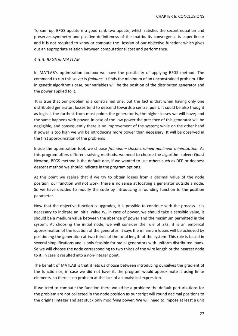
perturbation to avoid this problem in the derivatives estimation. At the same time, to make it
converge faster, we will modify escalate the power variable to change at a higher rate by
modifying the function’s code and remembering reconvert the result later on. In fact what we
are doing is limiting the range of powers and equilibrating the variable’s sort of data.
Figure 23. Modifications in MATLAB code
As we have forced high perturbations, we need to consider the possibility to get stuck around
the solution and getting inside an infinite buckle repeating the same iterations, so it is
necessary to limit the maximum number of iterations and tolerance.
We do not need to worry about the result obtained at this point, it is a good approximation. In
the next chapter we will improve these results, obtaining the real global minimum of the
problem.
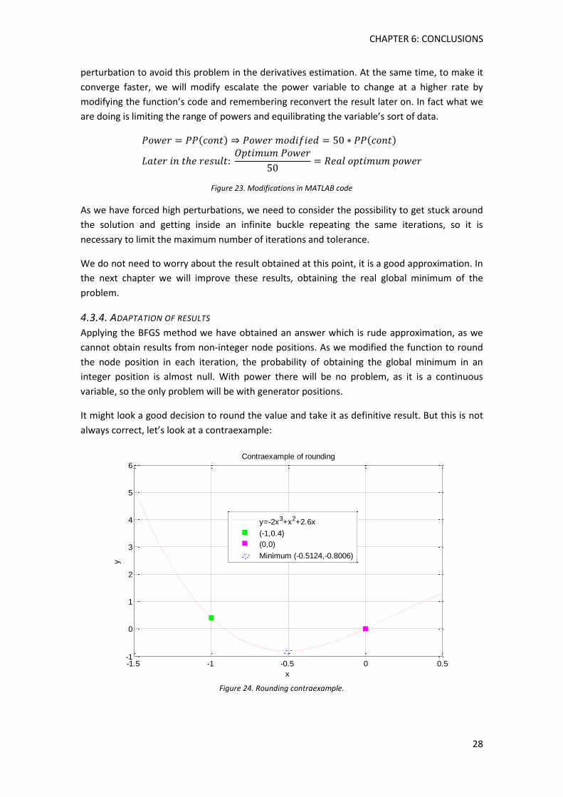
4.3.4. ADAPTATION OF RESULTS
Applying the BFGS method we have obtained an answer which is rude approximation, as we
cannot obtain results from non-integer node positions. As we modified the function to round
the node position in each iteration, the probability of obtaining the global minimum in an
integer position is almost null. With power there will be no problem, as it is a continuous
variable, so the only problem will be with generator positions.
It might look a good decision to round the value and take it as definitive result. But this is not
always correct, let’s look at a contraexample:
Figure 24. Rounding contraexample.
-1.5 -1 -0.5 0 0.5-1
0
1
2
3
4
5
6Contraexample of rounding
x
y
y=-2x3+x2+2.6x
(-1,0.4)
(0,0)
Minimum (-0.5124,-0.8006)
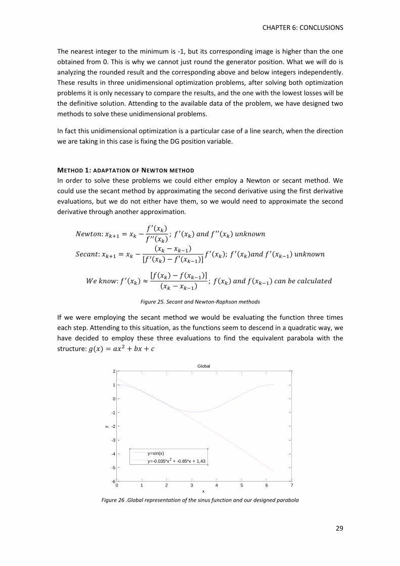
CHAPTER 6: CONCLUSIONS
29
The nearest integer to the minimum is -1, but its corresponding image is higher than the one
obtained from 0. This is why we cannot just round the generator position. What we will do is
analyzing the rounded result and the corresponding above and below integers independently.
These results in three unidimensional optimization problems, after solving both optimization
problems it is only necessary to compare the results, and the one with the lowest losses will be
the definitive solution. Attending to the available data of the problem, we have designed two
methods to solve these unidimensional problems.
In fact this unidimensional optimization is a particular case of a line search, when the direction
we are taking in this case is fixing the DG position variable.
METHOD 1: ADAPTATION OF NEWTON METHOD
In order to solve these problems we could either employ a Newton or secant method. We
could use the secant method by approximating the second derivative using the first derivative
evaluations, but we do not either have them, so we would need to approximate the second
derivative through another approximation.
[ ]
[ ]
Figure 25. Secant and Newton-Raphson methods
If we were employing the secant method we would be evaluating the function three times
each step. Attending to this situation, as the functions seem to descend in a quadratic way, we
have decided to employ these three evaluations to find the equivalent parabola with the
structure:
Figure 26 .Global representation of the sinus function and our designed parabola
0 1 2 3 4 5 6 7-6
-5
-4
-3
-2
-1
0
1
2
x
y
Global
y=sin(x)
y=-0.035*x2 + -0.85*x + 1,43
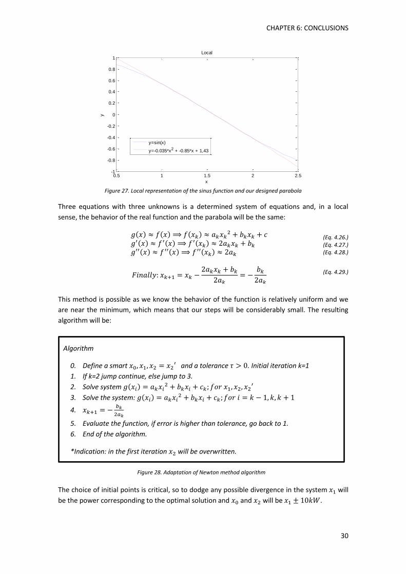
CHAPTER 6: CONCLUSIONS
30
Figure 27. Local representation of the sinus function and our designed parabola
Three equations with three unknowns is a determined system of equations and, in a local
sense, the behavior of the real function and the parabola will be the same:
(Eq. 4.26.) (Eq. 4.27.) (Eq. 4.28.)
(Eq. 4.29.)
This method is possible as we know the behavior of the function is relatively uniform and we
are near the minimum, which means that our steps will be considerably small. The resulting
algorithm will be:
Algorithm
0. Define a smart and a tolerance . Initial iteration k=1
1. If k=2 jump continue, else jump to 3.
2. Solve system
3. Solve the system:
4.
5. Evaluate the function, if error is higher than tolerance, go back to 1.
6. End of the algorithm.
*Indication: in the first iteration will be overwritten.
The choice of initial points is critical, so to dodge any possible divergence in the system will
be the power corresponding to the optimal solution and and will be .
0.5 1 1.5 2 2.5-1
-0.8
-0.6
-0.4
-0.2
0
0.2
0.4
0.6
0.8
1
x
y
Local
y=sin(x)
y=-0.035*x2 + -0.85*x + 1,43
Figure 28. Adaptation of Newton method algorithm
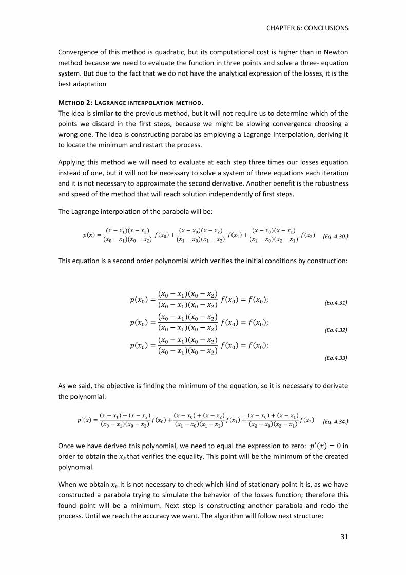
CHAPTER 6: CONCLUSIONS
31
Convergence of this method is quadratic, but its computational cost is higher than in Newton
method because we need to evaluate the function in three points and solve a three- equation
system. But due to the fact that we do not have the analytical expression of the losses, it is the
best adaptation
METHOD 2: LAGRANGE INTERPOLATION METHOD.
The idea is similar to the previous method, but it will not require us to determine which of the
points we discard in the first steps, because we might be slowing convergence choosing a
wrong one. The idea is constructing parabolas employing a Lagrange interpolation, deriving it
to locate the minimum and restart the process.
Applying this method we will need to evaluate at each step three times our losses equation
instead of one, but it will not be necessary to solve a system of three equations each iteration
and it is not necessary to approximate the second derivative. Another benefit is the robustness
and speed of the method that will reach solution independently of first steps.
The Lagrange interpolation of the parabola will be:
(Eq. 4.30.)
This equation is a second order polynomial which verifies the initial conditions by construction:
(Eq.4.31)
(Eq.4.32)
(Eq.4.33)
As we said, the objective is finding the minimum of the equation, so it is necessary to derivate
the polynomial:
(Eq. 4.34.)
Once we have derived this polynomial, we need to equal the expression to zero: in
order to obtain the that verifies the equality. This point will be the minimum of the created
polynomial.
When we obtain it is not necessary to check which kind of stationary point it is, as we have
constructed a parabola trying to simulate the behavior of the losses function; therefore this
found point will be a minimum. Next step is constructing another parabola and redo the
process. Until we reach the accuracy we want. The algorithm will follow next structure:
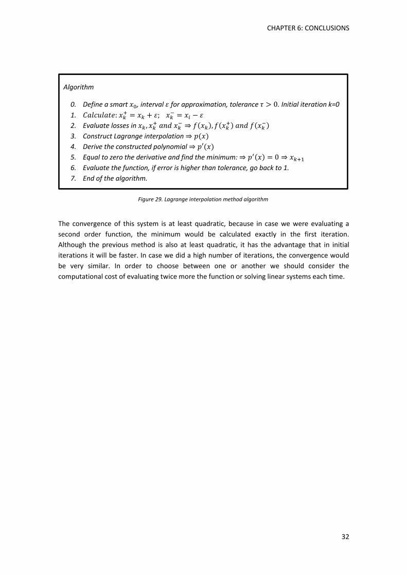
CHAPTER 6: CONCLUSIONS
32
Algorithm
0. Define a smart , interval for approximation, tolerance . Initial iteration k=0
1.
2. Evaluate losses in
3. Construct Lagrange interpolation
4. Derive the constructed polynomial
5. Equal to zero the derivative and find the minimum:
6. Evaluate the function, if error is higher than tolerance, go back to 1.
7. End of the algorithm.
The convergence of this system is at least quadratic, because in case we were evaluating a
second order function, the minimum would be calculated exactly in the first iteration.
Although the previous method is also at least quadratic, it has the advantage that in initial
iterations it will be faster. In case we did a high number of iterations, the convergence would
be very similar. In order to choose between one or another we should consider the
computational cost of evaluating twice more the function or solving linear systems each time.
Figure 29. Lagrange interpolation method algorithm
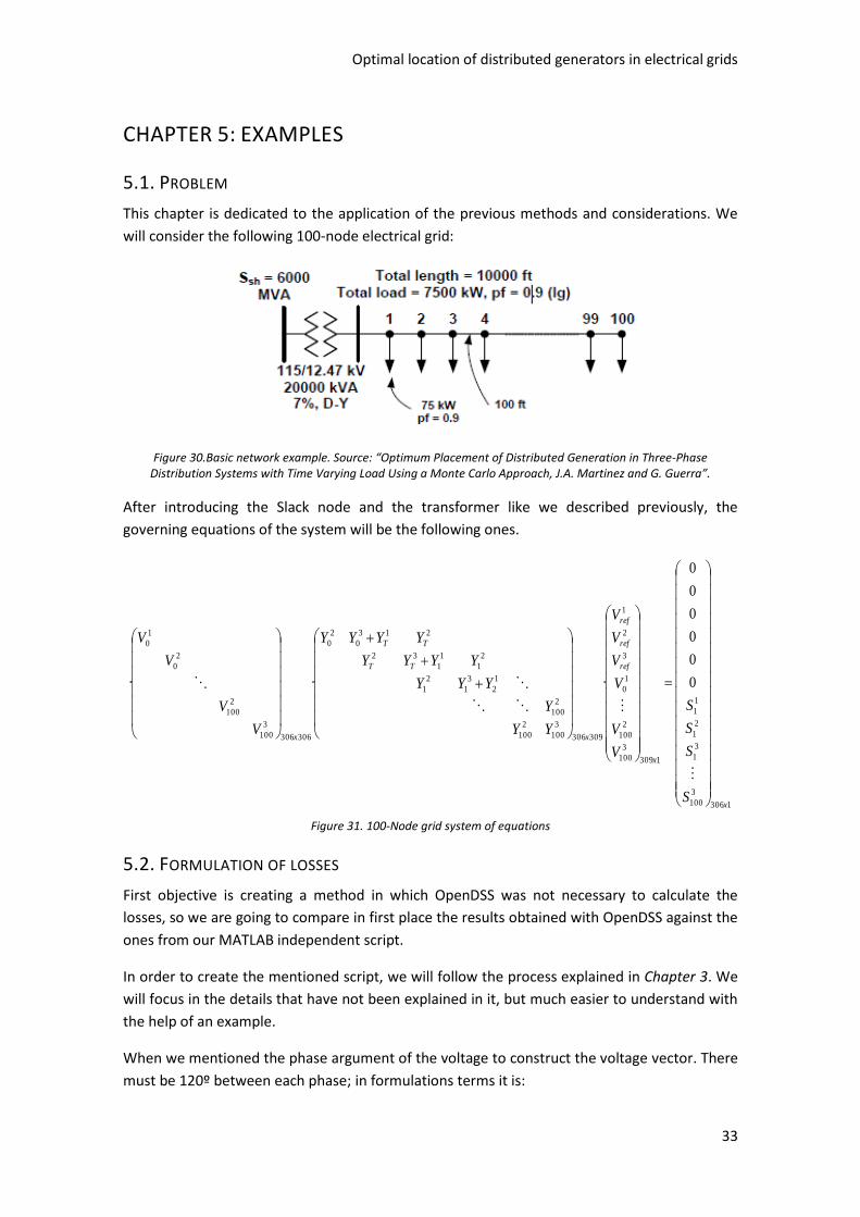
Optimal location of distributed generators in electrical grids
33
CHAPTER 5: EXAMPLES
5.1. PROBLEM
This chapter is dedicated to the application of the previous methods and considerations. We
will consider the following 100-node electrical grid:
Figure 30.Basic network example. Source: “Optimum Placement of Distributed Generation in Three-Phase Distribution Systems with Time Varying Load Using a Monte Carlo Approach, J.A. Martinez and G. Guerra”.
After introducing the Slack node and the transformer like we described previously, the
governing equations of the system will be the following ones.
1306
3
100
3
1
2
1
1
1
1309
3
100
2
100
1
0
3
2
1
309306
3
100
2
100
2
100
1
2
3
1
2
1
2
1
1
1
32
213
0
2
0
306306
3
100
2
100
2
0
1
0
0
0
0
0
0
0
···
x
x
ref
ref
ref
x
TT
TT
x
S
S
S
S
V
V
V
V
V
V
YY
Y
YYY
YYYY
YYYY
V
V
V
V
Figure 31. 100-Node grid system of equations
5.2. FORMULATION OF LOSSES
First objective is creating a method in which OpenDSS was not necessary to calculate the
losses, so we are going to compare in first place the results obtained with OpenDSS against the
ones from our MATLAB independent script.
In order to create the mentioned script, we will follow the process explained in Chapter 3. We
will focus in the details that have not been explained in it, but much easier to understand with
the help of an example.
When we mentioned the phase argument of the voltage to construct the voltage vector. There
must be 120º between each phase; in formulations terms it is:
CHAPTER 6: CONCLUSIONS
34
∠ (Eq. 5.1.)
We told we were given admittance matrices from the generator and the transformer, but the
line admittances could be calculated by ourselves. Attending to the article “An Open Source
Platform for Collaborating on Smart Grid Research, R.C. Dugan; T. E. McDermott”, the
structure of the matrices are the mentioned in the Equation 3.14. It is also revealed that they
are directly proportional to its length. As the 100 nodes are separated the same distance, all
the line matrices will be the same. And we will only need to compute the first one:
[ ] [ ] (Eq. 5.2.)
A final observation to understand the generated codes, which has not been commented
previously is the origin of the load curves, in the case of the generator and the nodes. In first
place, it is directly given and we load it in the script. In the case of the node demands it is
slightly different, as we are given 4 load curves instead of 100. It is a simplification as we are
classifying 4 kinds of demand. Each of the nodes will have assigned one of these load curves,
depending on the needs.
The rest of the elements in the codes are the steps explained in Chapter 3 but with different
notation. Looking at the comments in the scripts and in case of doubt to the size of the
elements, there is no problem at understanding the scripts.
To make the comparison easier we are launching OpenDSS from MATLAB, it is done by
activating the COM Server. We will do it by locating ourselves in the directory of OpenDSS with
the command console of Windows (cmd.exe) and executing the following command:
“Regsvr32 OpenDSSEngine.dll”. It is necessary each time we close or reset the computer. From
now on, we can perform calculations in MATLAB like if we were in OpenDSS, but being
introduced by the following function:
Figure 32. Necessary MALTAB commands
The proceeding of the method we are applying in this case is a very simplified Monte Carlo
approach. We generate 10 random pairs of distributed generator position and power, to
evaluate their behavior.
To analyze the quality of our method, in comparison with OpenDSS, we obtain the relative
errors between MATLAB and OpenDSS results in each of the ten cases, to verify if they are
acceptable. The files corresponding to the execution of these calculations will be
losses_snap.m and losses_time.m for the snapshot and time modes respectively.
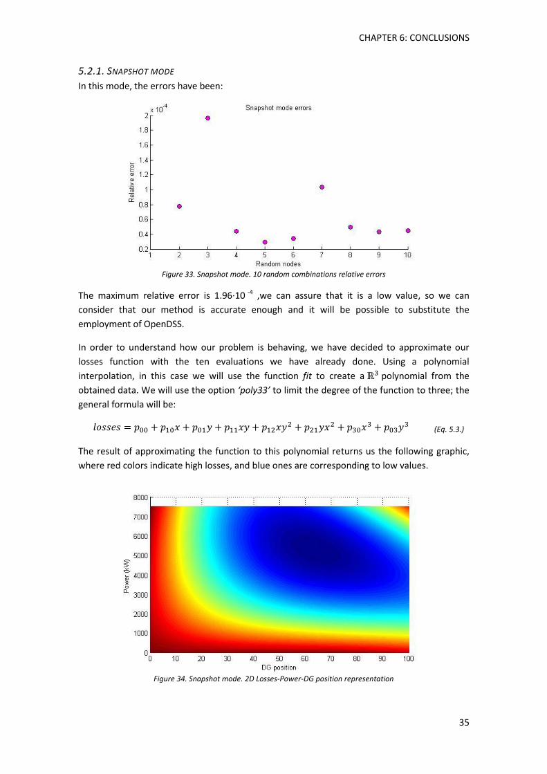
CHAPTER 6: CONCLUSIONS
35
5.2.1. SNAPSHOT MODE
In this mode, the errors have been:
Figure 33. Snapshot mode. 10 random combinations relative errors
The maximum relative error is 1.96·10 -4 ,we can assure that it is a low value, so we can
consider that our method is accurate enough and it will be possible to substitute the
employment of OpenDSS.
In order to understand how our problem is behaving, we have decided to approximate our
losses function with the ten evaluations we have already done. Using a polynomial
interpolation, in this case we will use the function fit to create a polynomial from the
obtained data. We will use the option ‘poly33’ to limit the degree of the function to three; the
general formula will be:
(Eq. 5.3.)
The result of approximating the function to this polynomial returns us the following graphic,
where red colors indicate high losses, and blue ones are corresponding to low values.
Figure 34. Snapshot mode. 2D Losses-Power-DG position representation
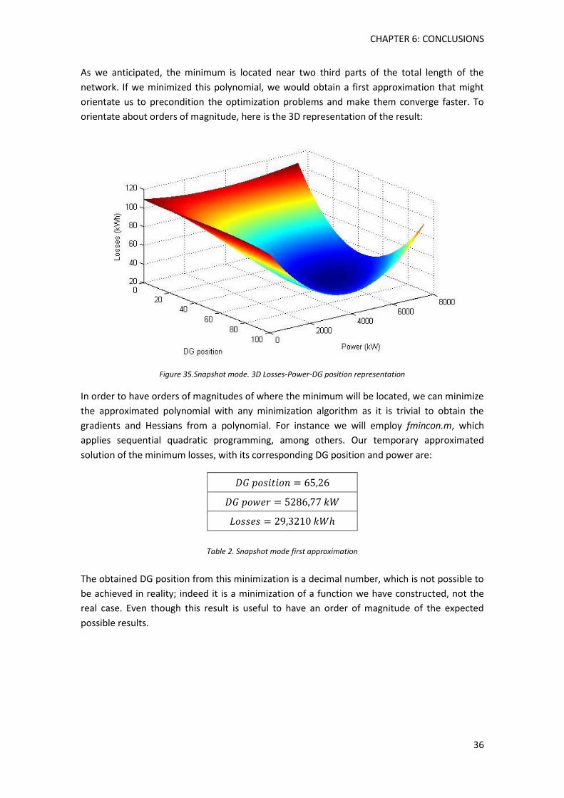
CHAPTER 6: CONCLUSIONS
36
As we anticipated, the minimum is located near two third parts of the total length of the
network. If we minimized this polynomial, we would obtain a first approximation that might
orientate us to precondition the optimization problems and make them converge faster. To
orientate about orders of magnitude, here is the 3D representation of the result:
Figure 35.Snapshot mode. 3D Losses-Power-DG position representation
In order to have orders of magnitudes of where the minimum will be located, we can minimize
the approximated polynomial with any minimization algorithm as it is trivial to obtain the
gradients and Hessians from a polynomial. For instance we will employ fmincon.m, which
applies sequential quadratic programming, among others. Our temporary approximated
solution of the minimum losses, with its corresponding DG position and power are:
Table 2. Snapshot mode first approximation
The obtained DG position from this minimization is a decimal number, which is not possible to
be achieved in reality; indeed it is a minimization of a function we have constructed, not the
real case. Even though this result is useful to have an order of magnitude of the expected
possible results.
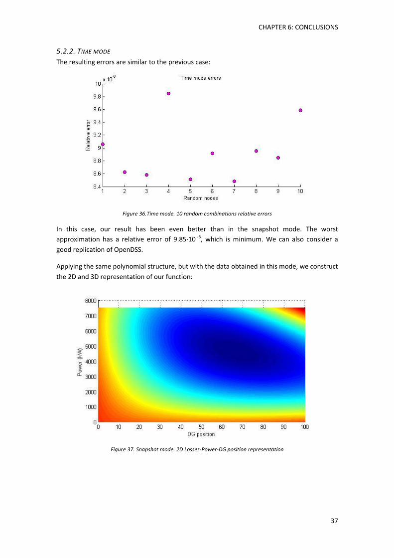
CHAPTER 6: CONCLUSIONS
37
5.2.2. TIME MODE
The resulting errors are similar to the previous case:
Figure 36.Time mode. 10 random combinations relative errors
In this case, our result has been even better than in the snapshot mode. The worst
approximation has a relative error of 9.85·10 -6, which is minimum. We can also consider a
good replication of OpenDSS.
Applying the same polynomial structure, but with the data obtained in this mode, we construct
the 2D and 3D representation of our function:
Figure 37. Snapshot mode. 2D Losses-Power-DG position representation
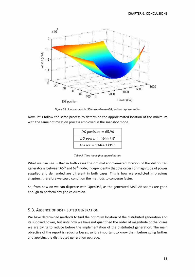
CHAPTER 6: CONCLUSIONS
38
Figure 38. Snapshot mode. 3D Losses-Power-DG position representation
Now, let’s follow the same process to determine the approximated location of the minimum
with the same optimization process employed in the snapshot mode.
Table 3. Time mode first approximation
What we can see is that in both cases the optimal approximated location of the distributed
generator is between 65th and 67th node; independently that the orders of magnitude of power
supplied and demanded are different in both cases. This is how we predicted in previous
chapters; therefore we could condition the methods to converge faster.
So, from now on we can dispense with OpenDSS, as the generated MATLAB scripts are good
enough to perform any grid calculation.
5.3. ABSENCE OF DISTRIBUTED GENERATION
We have determined methods to find the optimum location of the distributed generation and
its supplied power, but until now we have not quantified the order of magnitude of the losses
we are trying to reduce before the implementation of the distributed generation. The main
objective of the report is reducing losses, so it is important to know them before going further
and applying the distributed generation upgrade.
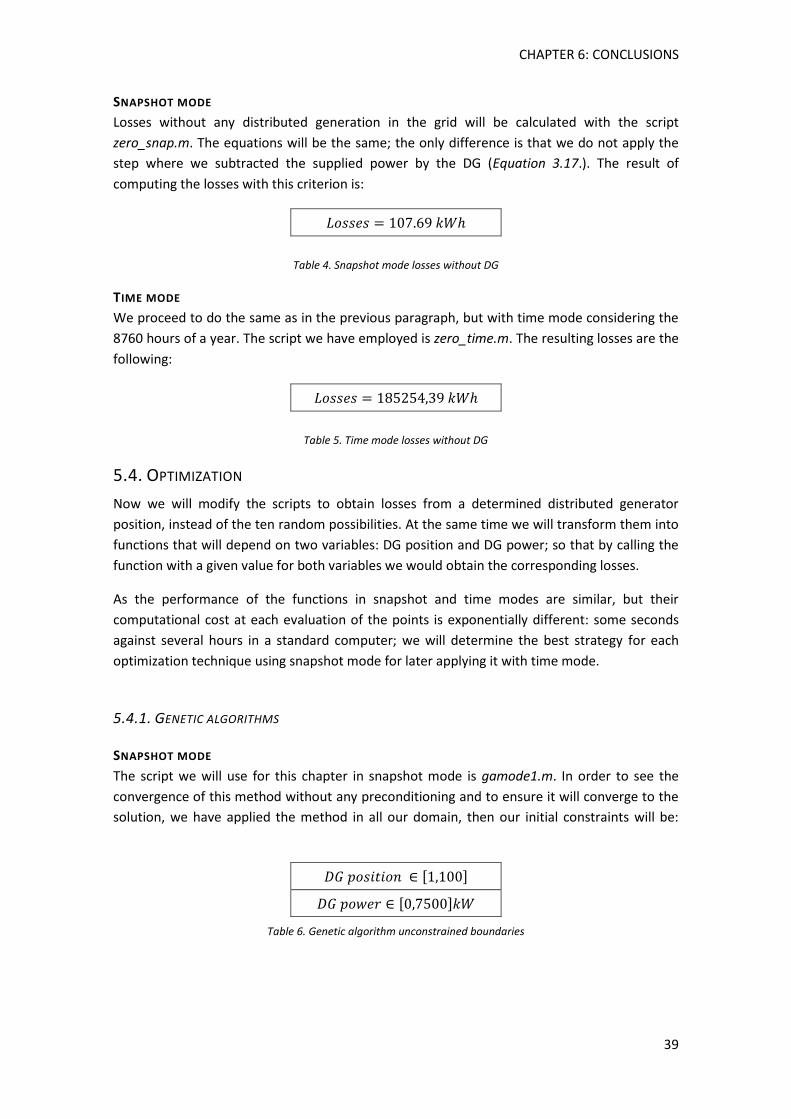
CHAPTER 6: CONCLUSIONS
39
SNAPSHOT MODE
Losses without any distributed generation in the grid will be calculated with the script
zero_snap.m. The equations will be the same; the only difference is that we do not apply the
step where we subtracted the supplied power by the DG (Equation 3.17.). The result of
computing the losses with this criterion is:
Table 4. Snapshot mode losses without DG
TIME MODE
We proceed to do the same as in the previous paragraph, but with time mode considering the
8760 hours of a year. The script we have employed is zero_time.m. The resulting losses are the
following:
Table 5. Time mode losses without DG
5.4. OPTIMIZATION
Now we will modify the scripts to obtain losses from a determined distributed generator
position, instead of the ten random possibilities. At the same time we will transform them into
functions that will depend on two variables: DG position and DG power; so that by calling the
function with a given value for both variables we would obtain the corresponding losses.
As the performance of the functions in snapshot and time modes are similar, but their
computational cost at each evaluation of the points is exponentially different: some seconds
against several hours in a standard computer; we will determine the best strategy for each
optimization technique using snapshot mode for later applying it with time mode.
5.4.1. GENETIC ALGORITHMS
SNAPSHOT MODE
The script we will use for this chapter in snapshot mode is gamode1.m. In order to see the
convergence of this method without any preconditioning and to ensure it will converge to the
solution, we have applied the method in all our domain, then our initial constraints will be:
[ ]
[ ]
Table 6. Genetic algorithm unconstrained boundaries
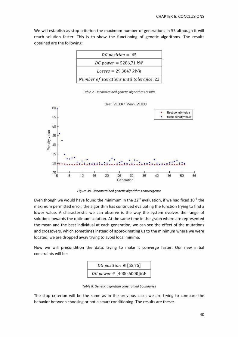
CHAPTER 6: CONCLUSIONS
40
We will establish as stop criterion the maximum number of generations in 55 although it will
reach solution faster. This is to show the functioning of genetic algorithms. The results
obtained are the following:
Table 7. Unconstrained genetic algorithms results
Figure 39. Unconstrained genetic algorithms convergence
Even though we would have found the minimum in the 22th evaluation, if we had fixed 10 -5 the
maximum permitted error; the algorithm has continued evaluating the function trying to find a
lower value. A characteristic we can observe is the way the system evolves the range of
solutions towards the optimum solution. At the same time in the graph where are represented
the mean and the best individual at each generation, we can see the effect of the mutations
and crossovers, which sometimes instead of approximating us to the minimum where we were
located, we are dropped away trying to avoid local minima.
Now we will precondition the data, trying to make it converge faster. Our new initial
constraints will be:
[ ]
[ ]
Table 8. Genetic algorithm constrained boundaries
The stop criterion will be the same as in the previous case; we are trying to compare the
behavior between choosing or not a smart conditioning. The results are these:
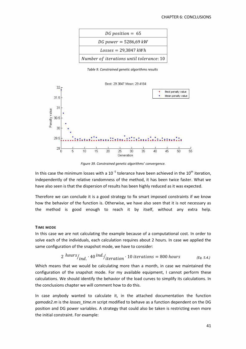
CHAPTER 6: CONCLUSIONS
41
Table 9. Constrained genetic algorithms results
Figure 39. Constrained genetic algorithms’ convergence.
In this case the minimum losses with a 10 -5 tolerance have been achieved in the 10th iteration,
independently of the relative randomness of the method, it has been twice faster. What we
have also seen is that the dispersion of results has been highly reduced as it was expected.
Therefore we can conclude it is a good strategy to fix smart imposed constraints if we know
how the behavior of the function is. Otherwise, we have also seen that it is not necessary as
the method is good enough to reach it by itself, without any extra help.
TIME MODE
In this case we are not calculating the example because of a computational cost. In order to
solve each of the individuals, each calculation requires about 2 hours. In case we applied the
same configuration of the snapshot mode, we have to consider:
⁄ ⁄ (Eq. 5.4.)
Which means that we would be calculating more than a month, in case we maintained the
configuration of the snapshot mode. For my available equipment, I cannot perform these
calculations. We should identify the behavior of the load curves to simplify its calculations. In
the conclusions chapter we will comment how to do this.
In case anybody wanted to calculate it, in the attached documentation the function
gamode2.m is the losses_time.m script modified to behave as a function dependent on the DG
position and DG power variables. A strategy that could also be taken is restricting even more
the initial constraint. For example:
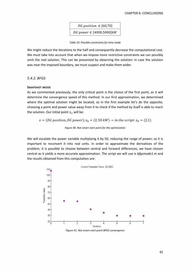
CHAPTER 6: CONCLUSIONS
42
[ ]
[ ]
Table 10. Possible constraints for time mode
We might reduce the iterations to the half and consequently decrease the computational cost.
We must take into account that when we impose more restrictive constraints we can possibly
omit the real solution. This can be prevented by observing the solution: in case the solution
was near the imposed boundary, we must suspect and make them wider.
5.4.2. BFGS
SNAPSHOT MODE
As we commented previously, the only critical point is the choice of the first point, as it will
determine the convergence speed of this method. In our first approximation, we determined
where the optimal solution might be located, so in the first example let’s do the opposite,
choosing a point and power value away from it to check if the method by itself is able to reach
the solution. Our initial point will be:
Figure 40. Not smart start point for the optimization
We will escalate the power variable multiplying it by 50, reducing the range of power; so it is
important to reconvert it into real units. In order to approximate the derivatives of the
problem, it is possible to choose between central and forward differences, we have chosen
central as it yields a more accurate approximation. The script we will use is bfgsmode1.m and
the results obtained from this computation are:
Figure 41. Not smart start point BFGS convergence
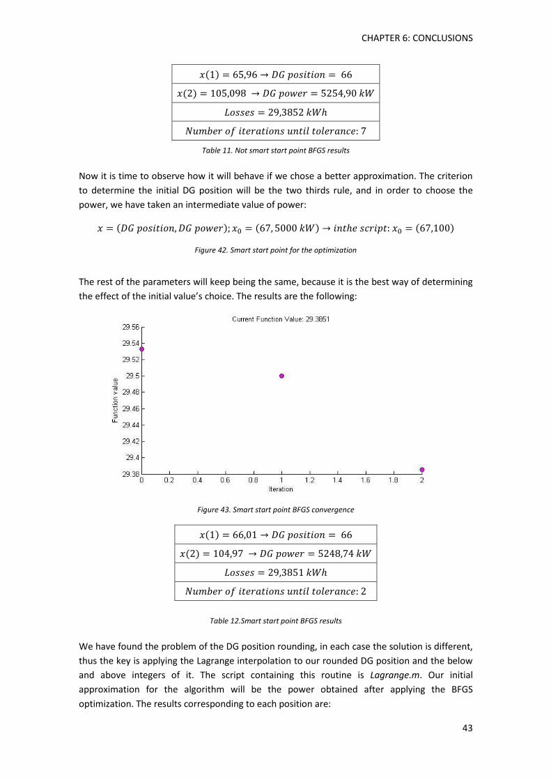
CHAPTER 6: CONCLUSIONS
43
Table 11. Not smart start point BFGS results
Now it is time to observe how it will behave if we chose a better approximation. The criterion
to determine the initial DG position will be the two thirds rule, and in order to choose the
power, we have taken an intermediate value of power:
Figure 42. Smart start point for the optimization
The rest of the parameters will keep being the same, because it is the best way of determining
the effect of the initial value’s choice. The results are the following:
Figure 43. Smart start point BFGS convergence
Table 12.Smart start point BFGS results
We have found the problem of the DG position rounding, in each case the solution is different,
thus the key is applying the Lagrange interpolation to our rounded DG position and the below
and above integers of it. The script containing this routine is Lagrange.m. Our initial
approximation for the algorithm will be the power obtained after applying the BFGS
optimization. The results corresponding to each position are:
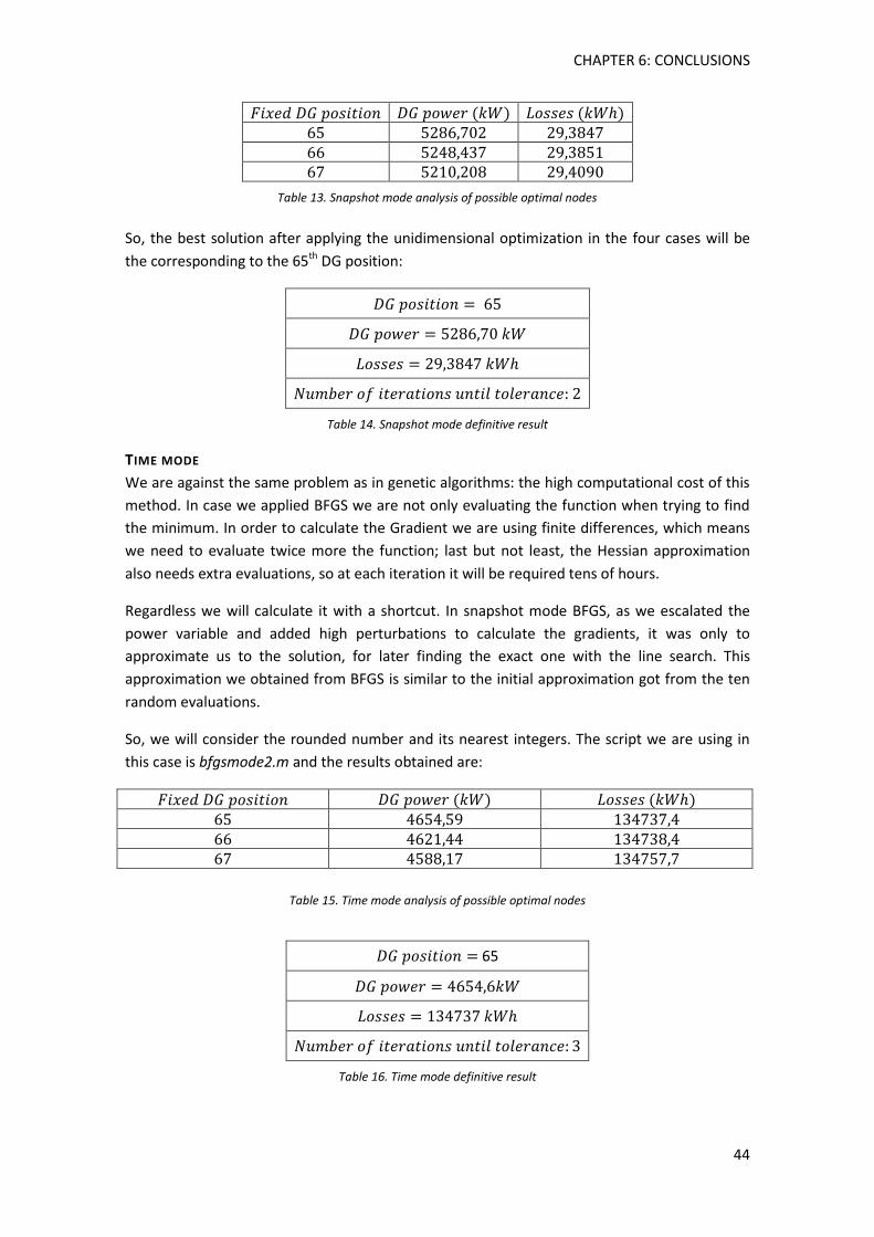
CHAPTER 6: CONCLUSIONS
44
Table 13. Snapshot mode analysis of possible optimal nodes
So, the best solution after applying the unidimensional optimization in the four cases will be
the corresponding to the 65th DG position:
Table 14. Snapshot mode definitive result
TIME MODE
We are against the same problem as in genetic algorithms: the high computational cost of this
method. In case we applied BFGS we are not only evaluating the function when trying to find
the minimum. In order to calculate the Gradient we are using finite differences, which means
we need to evaluate twice more the function; last but not least, the Hessian approximation
also needs extra evaluations, so at each iteration it will be required tens of hours.
Regardless we will calculate it with a shortcut. In snapshot mode BFGS, as we escalated the
power variable and added high perturbations to calculate the gradients, it was only to
approximate us to the solution, for later finding the exact one with the line search. This
approximation we obtained from BFGS is similar to the initial approximation got from the ten
random evaluations.
So, we will consider the rounded number and its nearest integers. The script we are using in
this case is bfgsmode2.m and the results obtained are:
Table 15. Time mode analysis of possible optimal nodes
65
Table 16. Time mode definitive result
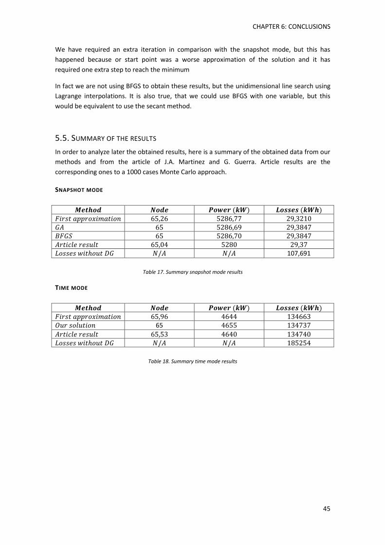
CHAPTER 6: CONCLUSIONS
45
We have required an extra iteration in comparison with the snapshot mode, but this has
happened because or start point was a worse approximation of the solution and it has
required one extra step to reach the minimum
In fact we are not using BFGS to obtain these results, but the unidimensional line search using
Lagrange interpolations. It is also true, that we could use BFGS with one variable, but this
would be equivalent to use the secant method.
5.5. SUMMARY OF THE RESULTS
In order to analyze later the obtained results, here is a summary of the obtained data from our
methods and from the article of J.A. Martinez and G. Guerra. Article results are the
corresponding ones to a 1000 cases Monte Carlo approach.
SNAPSHOT MODE
107,691
Table 17. Summary snapshot mode results
TIME MODE
65
Table 18. Summary time mode results
Optimal location of distributed generators in electrical grids
46
CHAPTER 6: CONCLUSIONS
6.1. OVERVIEWS
First of all, we have reached our main objective: reducing losses through the implementation
of Distributed Generation with Smart Grids support. Analyzing the results, we observe that
losses have been reduced up to the third of the original value. This fall, added to the other
benefits of Distributed Generation, such as favoring green energies and reducing dependence
of the system on an only source of energy, shows us that the implementation of Smart Grids
technology is a field with great potential.
We have also evaded the need of OpenDSS with the generated MATLAB codes. The advantage
of creating these independent codes is that we know exactly which calculations we are
performing, to modify it when our requirements change; instead of introducing data and
obtaining directly the results. As engineers, we are must be compelled to understand what we
are doing when solving problems
Both optimization systems have worked properly in a computational way, as they have leaded
us to the same result of the problem; so in this aspect the output has been successful. Later on
we will comment advantages and disadvantages from each, attending to the results we have
obtained in the examples.
6.2. ANALYSIS OF THE RESULTS
As we have been working with radial generators, the results have respected the rule of the two
thirds, locating the optimal DG position near two thirds parts of the total grid distance. In both
snapshot and time mode, it has been accomplished, so it does not depend on the power
supplied mode. This supposition is very helpful to solve problems faster.
It must be said that both methods have lead us to the same answer; it means that both of
them could be used to solve the problem. But let’s be stricter; the choice of two different
methods to solve a complex problem like this has been ideal to evaluate the weaknesses and
strengths of each.
GENETIC ALGORITHMS
+ Ideal for limiting the DG position to be an integer without affecting to the convergence
with rounding.
+ It is a robust method, independently of the initial conditions; we will reach the
optimum solution sooner or later.
+ In case we had a non-linear grid, we would jump away local minima.
- The DG power variable is a real value, so the possibilities are infinite; in our
calculations, this method loses effectiveness when determining the optimum power.
- Although we always converge to the solution because the algorithm evolves the
solutions, its initial speed is sometimes conditioned by a random factor.
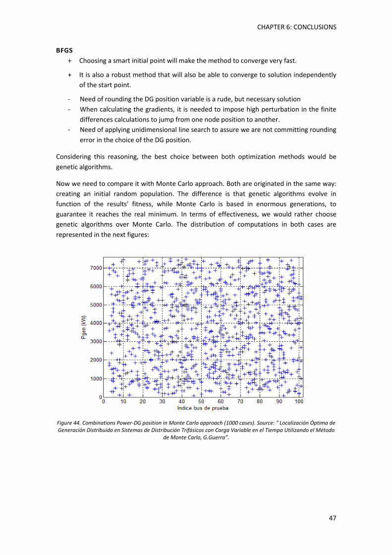
CHAPTER 6: CONCLUSIONS
47
BFGS
+ Choosing a smart initial point will make the method to converge very fast.
+ It is also a robust method that will also be able to converge to solution independently
of the start point.
- Need of rounding the DG position variable is a rude, but necessary solution
- When calculating the gradients, it is needed to impose high perturbation in the finite
differences calculations to jump from one node position to another.
- Need of applying unidimensional line search to assure we are not committing rounding
error in the choice of the DG position.
Considering this reasoning, the best choice between both optimization methods would be
genetic algorithms.
Now we need to compare it with Monte Carlo approach. Both are originated in the same way:
creating an initial random population. The difference is that genetic algorithms evolve in
function of the results’ fitness, while Monte Carlo is based in enormous generations, to
guarantee it reaches the real minimum. In terms of effectiveness, we would rather choose
genetic algorithms over Monte Carlo. The distribution of computations in both cases are
represented in the next figures:
Figure 44. Combinations Power-DG position in Monte Carlo approach (1000 cases). Source: " Localización Óptima de Generación Distribuida en Sistemas de Distribución Trifásicos con Carga Variable en el Tiempo Utilizando el Método
de Monte Carlo, G.Guerra”.
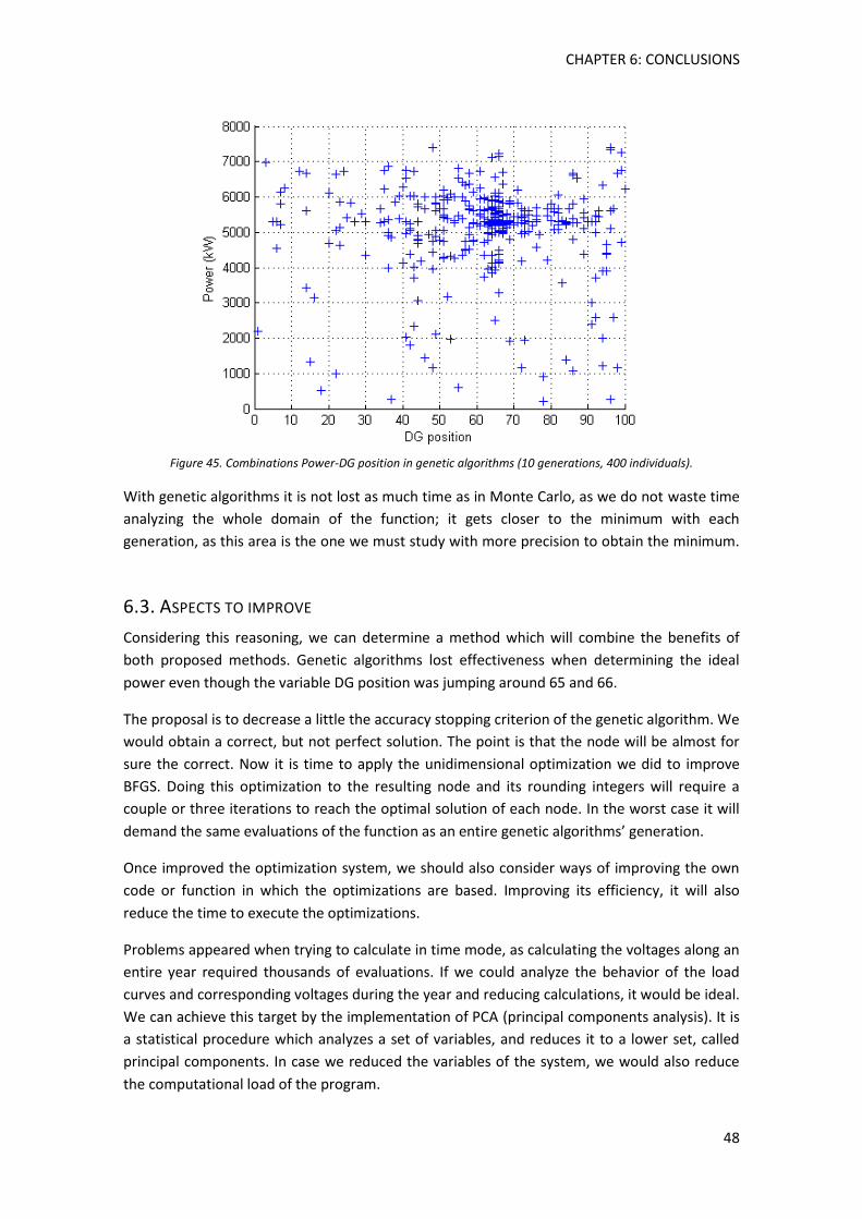
CHAPTER 6: CONCLUSIONS
48
Figure 45. Combinations Power-DG position in genetic algorithms (10 generations, 400 individuals).
With genetic algorithms it is not lost as much time as in Monte Carlo, as we do not waste time
analyzing the whole domain of the function; it gets closer to the minimum with each
generation, as this area is the one we must study with more precision to obtain the minimum.
6.3. ASPECTS TO IMPROVE
Considering this reasoning, we can determine a method which will combine the benefits of
both proposed methods. Genetic algorithms lost effectiveness when determining the ideal
power even though the variable DG position was jumping around 65 and 66.
The proposal is to decrease a little the accuracy stopping criterion of the genetic algorithm. We
would obtain a correct, but not perfect solution. The point is that the node will be almost for
sure the correct. Now it is time to apply the unidimensional optimization we did to improve
BFGS. Doing this optimization to the resulting node and its rounding integers will require a
couple or three iterations to reach the optimal solution of each node. In the worst case it will
demand the same evaluations of the function as an entire genetic algorithms’ generation.
Once improved the optimization system, we should also consider ways of improving the own
code or function in which the optimizations are based. Improving its efficiency, it will also
reduce the time to execute the optimizations.
Problems appeared when trying to calculate in time mode, as calculating the voltages along an
entire year required thousands of evaluations. If we could analyze the behavior of the load
curves and corresponding voltages during the year and reducing calculations, it would be ideal.
We can achieve this target by the implementation of PCA (principal components analysis). It is
a statistical procedure which analyzes a set of variables, and reduces it to a lower set, called
principal components. In case we reduced the variables of the system, we would also reduce
the computational load of the program.
CHAPTER 6: CONCLUSIONS
49
CHAPTER 7: REFERENCES
Dugan, R., EPRI, K. T., & McDermott, T. (2011). An open source platform for collaborating on
smart grid research. San Diego, CA: Power and Energy Society General Meeting, 2011
IEEE.
Goldberg, D. E. (1989). Genetic Algorithms in Search, Optimization and Machine Learning.
Boston, MA: Addison-Wesley Longman Publishing Co., Inc.
Guerra Sánchez, L. G. (2012). Localización Óptima de Generación Distribuida en Sistemas de
Distribución Trifásicos con Carga Variable en el Tiempo Utilizando el Método de Monte
Carlo. Barcelona.
Haup, R. L. (2004). Practical Genetic Algorithms. Hoboken, New Jersey: John Wiley & Sons, Inc.
Martinez, J. A., & Guerra, G. (2012). Optimum Placement of Distributed Generation in Three-
Phase Distribution Systems with Time Varying Load Using a Monte Carlo Approach.
Power and Energy Society General Meeting, 2012 IEEE, 1-7.
Matthies, H., & Strang, G. (1979). The solution of nonlinear finite element equations. John
Wiley & Sons, Ltd.
Nguyen, H. L. (2002). Newton-Raphson method in complex form. IEEE Transactions on Power
Systems (Volume: 12 , Issue: 3 ) , 1355 - 1359.
Nocedal, J. (1980). Updating Quasi-Newton Matrices with Limited Storage. Mathematicals of
computation, Vol 35, No. 151, 773-782.
Numèric, L. d. (2012). Simulating and optimizing electrical grids: problem statement and
potential applications of ROM and PGD to Smart Grids. Universitat Politècnica de
Catalunya.
Ramírez, I. J., Martínez, J. A., Fuentes, J. A., García, E., Fernández, L. A., & Zorzano, P. J. (2007).
Problemas resueltos de sistema de energía eléctrica. Madrid, España: International
Thomson Editores Espain.
University of Newcastle. (n.d.). Retrieved from http://www.edc.ncl.ac.uk
Wasley, R., & Shlash, M. (2010). Newton-Raphson algorithm for 3-phase load flow. Proceedings
of the Institution of Electrical Engineers (Volume:121 , Issue: 7 ), 630-638.
Wikipedia. (n.d.). Retrieved from http://en.wikipedia.org/


![ANALYSIS OF THE BFGS METHOD WITH ERRORSAs was shown by Powell [15], an Armijo-Wolfe line search guarantees the stability of the BFGS updating procedure, and ultimately the global convergence](https://img.pdfslide.us/doc/110x75/5faedafa340ac25373429f76/analysis-of-the-bfgs-method-with-as-was-shown-by-powell-15-an-armijo-wolfe-line.jpg)