1

L-BFGS and Delayed Dynamical Systems Approach for Unconstrained Optimization

Xiaohui XIE

Supervisor: Dr. Hon Wah TAM

2

Outline

Problem background and introduction Analysis for dynamical systems with time delay

Introduction of dynamical systems Delayed dynamical systems approach Uniqueness property of dynamical systems

Numerical testing Main stages of this research APPENDIX

3

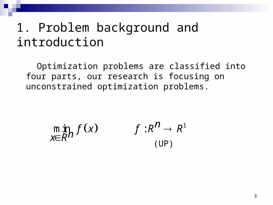
1. Problem background and introduction

Optimization problems are classified into four parts, our research is focusing on unconstrained optimization problems.

(UP)

1min : nf x f R Rnx R

4

Descent direction

A common theme behind all these methods is to find a direction so that there exists an such that

np x R 0

.,0 xfpxf

5

Steepest descent method

For (UP), is a descent direction at

or is a descent direction for .

p

0T

f x p

x

xfp 2

/ xfxfp f x

6

Method of Steepest Descent

Find that solves

Then

Unfortunately, the steepest descent method converges only linearly, and sometimes very slowly linearly.

k .min0

kk xfxf

1 .k k k kx x f x

7

Newton’s method

Newton’s direction— Newton’s method

Given , compute

Although Newton’s method converges very fast, the Hessian matrix is difficult to compute.

kk xfxf 12

0x 12

1 ,k k k kx x f x f x

1.k k

8

Quasi-Newton method—BFGS

Instead of using the Hessian matrix, the quasi-Newton methods approximate it.

In quasi-Newton methods, the inverse of the Hessian matrix is approximated in each iteration by a positive definite (p.d.) matrix, say .

being symmetric and p.d. implies the descent property.

kH

k k kp H f x

kH

9

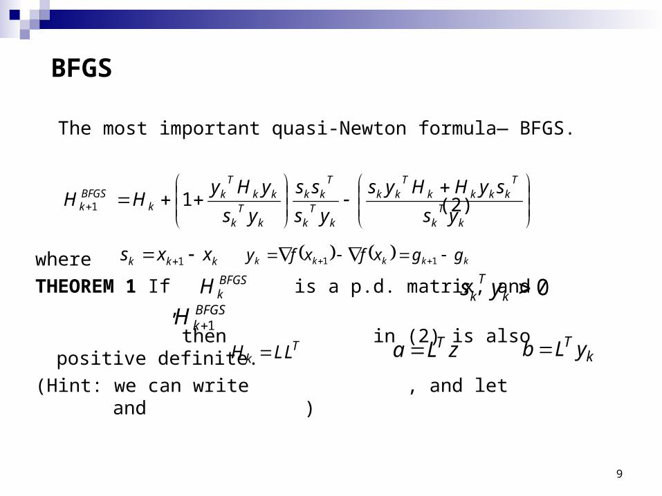
BFGS

The most important quasi-Newton formula— BFGS.

(2)

where

THEOREM 1 If is a p.d. matrix, and ,

then in (2) is also positive definite.

(Hint: we can write , and let and )

kT

k

Tkkkk

Tkk

kT

k

Tkk

kT

k

kkT

kk

BFGSk

ys

syHHys

ys

ss

ys

yHyHH 11

BFGSkH 0k

Tk ys

BFGSkH 1

TkH LL Ta L z T

kb L y

kkk xxs 1 kkkkk ggxfxfy 11

10

Limited-Memory Quasi-Newton Methods —L-BFGS

Limited-memory quasi-Newton methods are useful for solving large problems whose Hessian matrices cannot be computed at a reasonable cost or are not sparse.

Various limited-memory methods have been proposed; we focus mainly on an algorithm known as L-BFGS.

(3)

Tkkkkk

Tkk ssVHVH 1

Tkkkk

kT

k

k syIVsy

,1

kkk xxs 1 kkk ffy 1

11

The L-BFGS approximation satisfies the following formula:

for

(6)

for

(7)

mk 11 1 0 0 0 1

1 0 0 0 1

1 2 2 2 1

1 1 1

.

T T Tk k k k k

T T Tk k

T T Tk k k k k k k

T Tk k k k k

Tk k k

H V V V H V V V

V V s s V V

V V s s V V

V s s V

s s

mk 1 1 1 1 0 1 1

2 1 1 1 2

1 2 2 2 1

1 1 1

.

T T Tk k k k m k m k k

T T Tk k m k m k m k m k m k

T T Tk k k k k k k

T Tk k k k k

Tk k k

H V V V H V V V

V V s s V V

V V s s V V

V s s V

s s

1kH

12

2. Analysis for dynamical systems with time delay

The unconstrained problem (UP) is reproduced. (8)

It is very important that the optimization problem is posted in the continuous form, i.e. x can be changed continuously.

The conventional methods are addressed in the discrete form.

1min :n

n

x Rf x f R R

13

Dynamical system approach

The essence of this approach is to convert (UP) into a dynamical system or an ordinary differential equation (o.d.e.) so that the solution of this problem corresponds to a stable equilibrium point of this dynamical system.

Neural network approach

The mathematical representation of neural network is an ordinary differential equation which is asymptotically stable at any isolated solution point.

14

Consider the following simple dynamical system or ode

(9)

DEFINITION 1. (Equilibrium point). A point is called an equilibrium point of (9) if .

DEFINITION 3. (Convergence). Let be the solution of (9). An isolated equilibrium point is convergent if there exists a such that if , as .

xpdt

tdx

* nx R * 0p x

x t*x 0

*0x t x *x t x t

15

Some Dynamical system versions

Based on the steepest descent direction

Based on the Newton’s direction

Other dynamical systems

dxf x t

dt

12dx tf x t f x t

dt

dx ts t p x t

dt

2

2

d x t dx ta t b t B x t p x t

dt dt

16

Dynamical system approach can solve very large problems.

How to find a “good” ? The dynamical system approach normally consists of the

following three steps: to establish an ode system to study the convergence of the solution of the ode as

; and to solve the ode system numerically.

Even though the solutions of ode systems are continuous, the actual computation has to be done discretely.

p x

x t

t

17

Delayed dynamical systems approach

steepest

descent

direction

slow convergence

Newton’s

direction

difficult to compute

fast convergence and easy to calculate

18

The delayed dynamical systems approach solves the delayed o.d.e. (13)

For , we use

(13A)

Where

To compute at .

,( ( ), ( ( )), ..., ( ( ))) ( )1dx t

H x t x t t x t t f x tmdt

1mt t

1 0 1 1 0

1 2 1 1 2 0 1 0 0 1 1 2 2 1 1

1 2 1 1 2 0 1 0 1 0 1 1 2 2 1 1

1 2 1 2 1 2 1 1

1 1 1

, , , : , , , ,

:

.

m m m

T T T T

m m m m m m

T T T T

m m m m m m

T T

m m m m m m m m

T

m m m

H x t x t x t H x t x t x t x t

V t V t V t V t H V t V t V t V t

V t V t V t t s t s t V t V t V t

V t t s t s t V t

t s t s t

1 1 1 1

1 1 1 11

1 1

,

1, .

m m m m

T

m m m mT m

m m

s t x t x t y t f x t f x t

t V t I t y t s ty t s t

mx mt

19

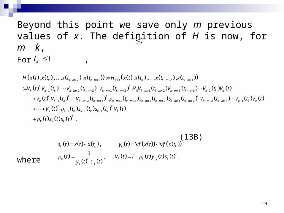
Beyond this point we save only m previous values of x. The definition of H is now, for m k,

For ,

(13B)

where

kt t

2 1 1 2 1

1 2 3 1 2 0 1 2 2 3 1

1 2 3 1 2 1 2 1 2 2

, , , , : , , , ,

:

k k m k m k k k m k m

T T T T

k k k k m k m k m k m k m k m k m k m k k k

T T T T

k k k k m k m k m k m k m k m k m k m k m

H x t x t x t x t H x t x t x t x t

V t V t V t V t H V t V t V t V t

V t V t V t t s t s t V

3 1

1 1 1

.

k m k k k

T T

k k k k k k k k

T

k k k

t V t V t

V t t s t s t V t

t s t s t

,

1, .

k k k k

T

k k k kT k

k k

s t x t x t y t f x t f x t

t V t I t y t s ty t s t

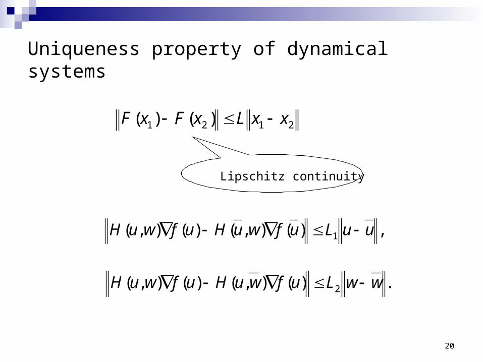
Uniqueness property of dynamical systems

20

2121 )()( xxLxFxF

Lipschitz continuity

,)(),()(),( 1 uuLufwuHufwuH

.)(),()(),( 2 wwLufwuHufwuH

Lemma 2.6

Let be continuously differentiable in the open convex set , and let be Lipschitz continuous at in the neighborhood using a vector norm and the induced matrix operator norm and the Lipschitz constant . Then, for any

: n mF R R,nD R x D F

Jx

x D

,x p D

2( ) ( ) ( )

2F x p F x J x p p

3. Numerical testing

Test problems

● Extended Rosenbrock function

● Penalty function Ⅰ● Variable dimensioned function

● Linear function-rank 1

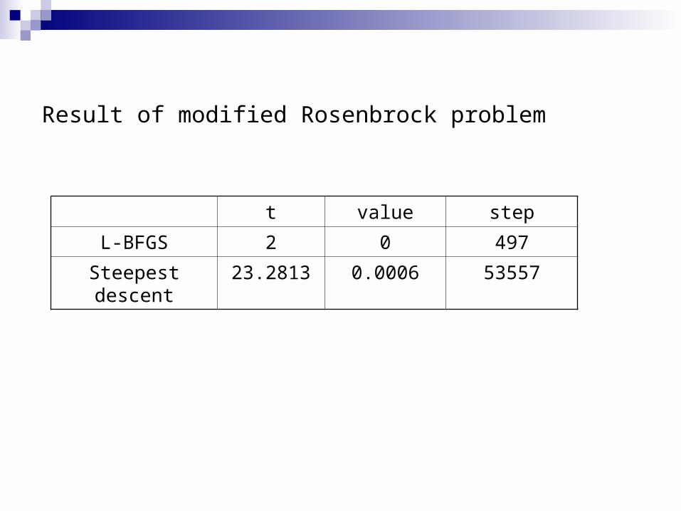
Result of modified Rosenbrock problem

t value step

L-BFGS 2 0 497

Steepest descent 23.2813 0.0006 53557

Comparison of function value

m = 2

m = 4

m = 6

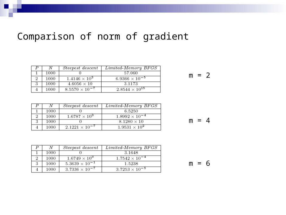
Comparison of norm of gradient

m = 2

m = 4

m = 6

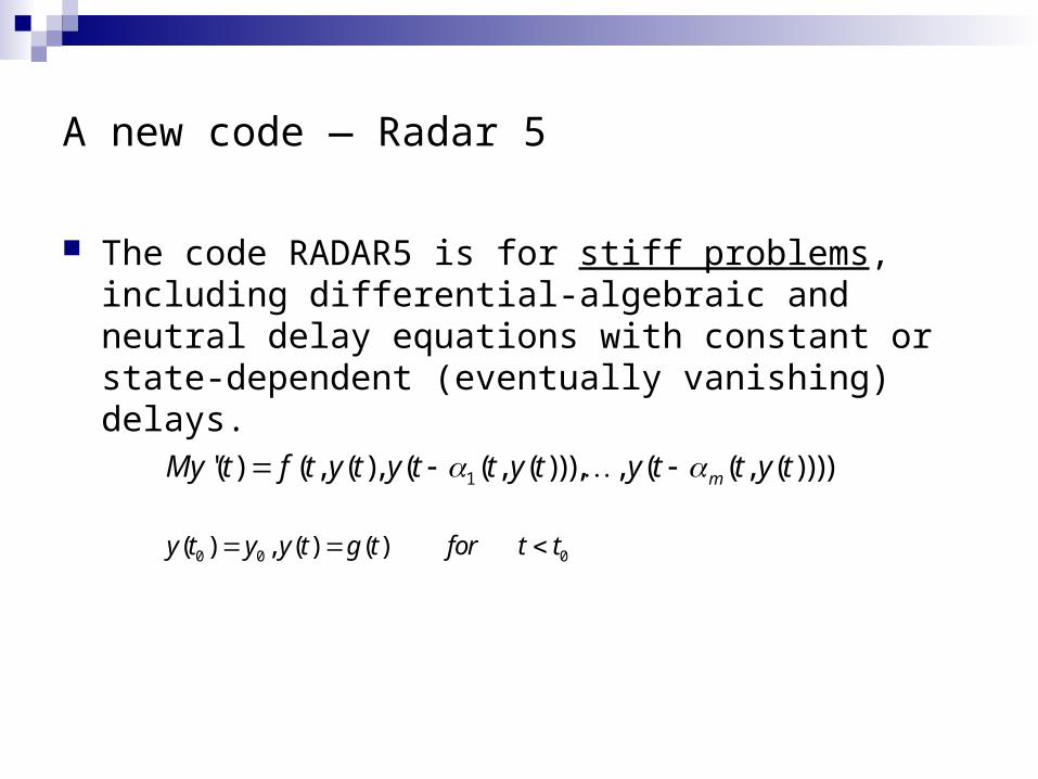
A new code — Radar 5

The code RADAR5 is for stiff problems, including differential-algebraic and neutral delay equations with constant or state-dependent (eventually vanishing) delays.

1'( ) ( , ( ), ( ( , ( ))), , ( ( , ( ))))mMy t f t y t y t t y t y t t y t

0 0 0( ) , ( ) ( )y t y y t g t for t t

27

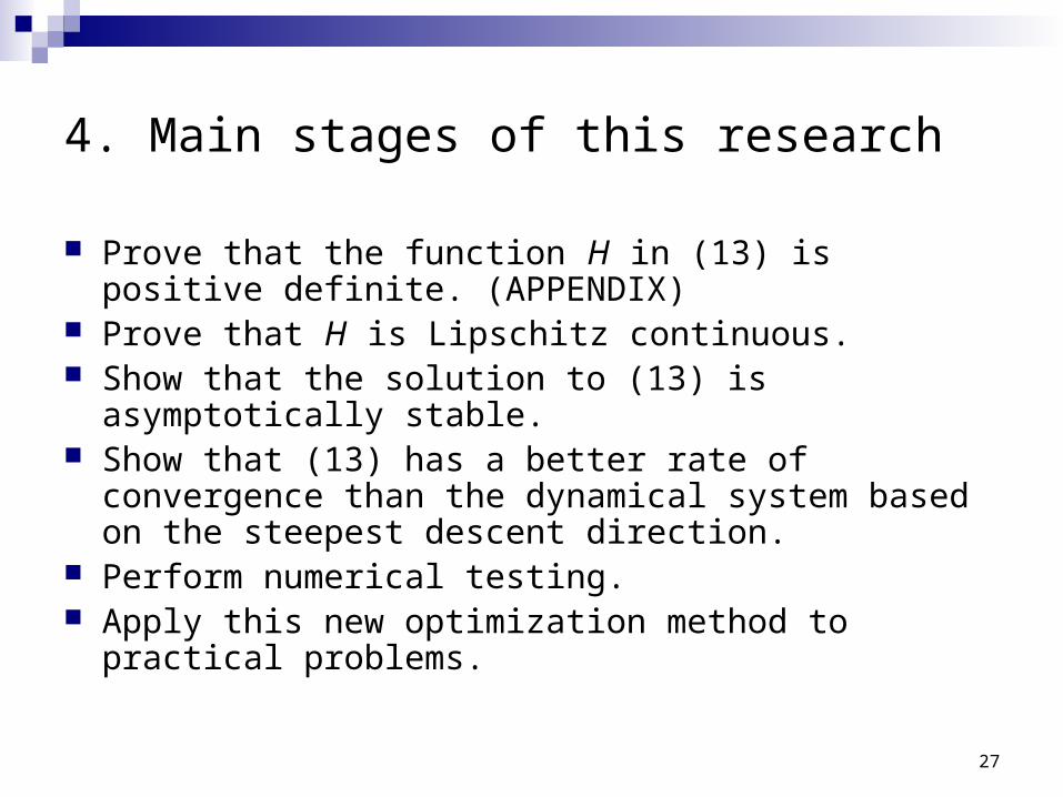
4. Main stages of this research

Prove that the function H in (13) is positive definite. (APPENDIX)

Prove that H is Lipschitz continuous. Show that the solution to (13) is asymptotically stable. Show that (13) has a better rate of convergence than the

dynamical system based on the steepest descent direction.

Perform numerical testing. Apply this new optimization method to practical

problems.

28

APPENDIX To show that H in (13) is positive definite

Property 1. If is positive definite, the matrix defined by (13) is positive definite (provided for all ).

I proved this result by induction. Since the continuous analog of the L-BFGS formula has two cases, the proof needs to cater for each of them.

0H

0iT

i sy iH

29

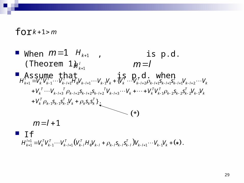
for

When , is p.d. (Theorem 1) Assume that is p.d. when

If

1k m

1m 1kH

1lkH

m l

1m l

1 1 1 0 1 1 2 1 1 1 2

3 2 2 2 3 1 2 2 2 1

1 1 1

{

}.

l T T T T T Tk k k k l k l k k k k l k l k l k l k l k

T T T T T Tk k l k l k l k l k l k k k k k k k k

T T Tk k k k k k k k

H V V V H V V V V V s s V V

V V s s V V V V s s V V

V s s V s s

*

11 1 1 0 1 1 .l T T T T T

k k k k l k l k l k l k l k l k l k kH V V V V H V s s V V V

30

for

In this case there is no exists.

By the assumption is p.d., it is obvious that

is also p.d..

1k m

m

1T T

k k k k k k kH V H V s s

kH1kH

31