Optimal local well-posedness theory for the kinetic wave equation

Pierre Germain ∗ Alexandru D. Ionescu† Minh-Binh Tran‡

November 15, 2017

Abstract

We prove local existence and uniqueness results for the (space-homogeneous) 4-wavekinetic equation in wave turbulence theory. We consider collision operators defined by radial,but general dispersion relations satisfying suitable bounds, and we prove two local well-posedness theorems in nearly critical weighted spaces.

Keyword: wave (weak) turbulence, quantum Boltzmann, nonlinear Schrodinger, wave kineticequations

MSC: 35BXX ; 37K05 ; 35Q55 ; 35C07; 45G05 ; 35Q20 ; 35B40 ; 35D30

Contents

1 Introduction 2

2 Main results 6

3 Proof of Proposition 2.3: L∞s (s > 2) boundedness of Tj 8

4 Proof of Proposition 2.4: L2s(s > 1/2) boundedness of Tj 14

5 Proof of Theorems 2.1 and 2.2 19

6 Further results 21

∗Courant Institute of Mathematical Sciences, 251 Mercer Street, New York, NY 10012, USA.Email: pgermain@cims.nyu.edu†Department of Mathematics, Fine Hall, Washington Road, Princeton, NJ 08544, USA.

Email: aionescu@math.princeton.edu‡Department of Mathematics, University of Wisconsin-Madison, Madison, WI 53706, USA.

Email: mtran23@wisc.edu

1

1 Introduction

1.1 Weak turbulence

Turbulence, as being understood today, describes the chaotic behavior of systems being in statesfar away from thermodynamic equilibrium and having a large number of degrees of freedom.It is not restrictive to hydrodynamics to be the only place where one can observe turbulence.Recent advances in plasma physics, acoustics, superconductivity, nonlinear optics, and ferroma-gentism have shown that turbulence is a universal phenomenon, which can be observed bothexperimentally and naturally. Such turbulence systems can be studied under the framework ofHamiltonian mechanics. In weak turbulence, the Hamiltonian can be expanded in an infinitepower series of normal variables, starting with quadratic terms. That means one usually be-gins with a linear system of non-interacting small amplitude waves and the nonlinear terms aretreated using a perturbation methods. The nonlinear effects then lead to the stochastization ofwaves phases and a slow modulation of the amplitudes. A kinetic equation of quantum Boltz-mann types for the mean square amplitudes can then be written. There are two common typesof such kinetic equations: the 3-wave and the 4-wave ones. The first derivation of a kinetic modelof weak turbulence, which is a 3-wave one, was obtained, to our knowledge, in [51, 52] in thestudy of phonon interactions in anharmonic crystal lattices. We refer to [65, 43, 63, 20, 44, 45]for detailed discussions on the topics.

4-wave kinetic equations play an important role in the theory of weak turbulence and appearin several contexts: gravity and capillary waves on the surface of a finite-depth fluid [64, 26,27, 28, 12], Alfven wave turbulence in astrophysical plasmas [46], optical waves of diffraction innonlinear media [13, 40, 41], quantum fluids [33], Langmuir waves [62] to name only a few.

1.2 The kinetic wave equation and its first properties

The present article investigates the local well-posedness theory for the space-homogeneous 4-wave kinetic equation

∂tf(t, p) = Q[f ](t, p), on R+ × R3,

f(0, p) =f0(p) on R3.(1.1)

The trilinear operator Q is given by

Q[f ](p) =

˚R3×3

δ(p+ p1− p2− p3)δ(ω+ω1−ω2−ω3)[f2f3(f1 + f)− ff1(f2 + f3)] dp1 dp2 dp3,

where we denoted

ω = ω(p), ωi = ω(pi), f = f(p), fi = f(pi).

In the above, p 7→ ω(p) is the dispersive relation of the underlying dispersive problem, to whichwe will come back shortly.

2

Notice that the nonlinear term can also be written

Q[f ](p) =

˚R3×3

δ(p+ p1 − p2 − p3)δ(ω + ω1 − ω2 − ω3)

× ff1f2f3

[ 1

f+

1

f1− 1

f2− 1

f3

]dp1 dp2 dp3.

Writing the nonlinear term in this way makes it clear that the mass, momentum, and energyare conserved; they are defined respectively as

ˆR3

f(p) dp,

ˆR3

pf(p) dp,

ˆR3

ω(p)f(p) dp.

Furthermore, the entropy, defined by

ˆR3

log f(p) dp,

is decreasing. Finally, the above form of the nonlinear term leads to the stationary solu-tions

1

µ+ ν · p+ ξω(p), (1.2)

where (µ, ν, ξ) ∈ R× R3 × R are such that µ+ ν · p+ ξω(p) ≥ 0 for any p.

The equation (1.1) does not admit invariant scalings for general dispersion relations ω(p). How-ever, for ω(p) = |p|2, a number of scalings arises, which leave the set of solutions invariant. Themost relevant one leaves the time variable untouched: it is given by the transformation

f(t, p) 7→ λ2f(t, λp). (1.3)

1.3 The dispersion relation

One of our aims is to allow more general dispersion relations which enjoy similar bounds toω(p) = |p|2. This is motivated by the following instances of physical interest:

• The basic example is the Schrodinger case

ω(p) = |p|2. (1.4)

• The Bogoliubov dispersion law [14, 45]

ϑ(p) =√θ1|p|2 + θ2|p|4, (1.5)

where θ1, θ2 are strictly positive constants.

3

• The modified Bogoliubov dispersion law [14] and the Bohm-Pines dispersion law [5]

ϑ(p) =√θ0 + θ1|p|2 + θ2|p|4, (1.6)

where θ0, θ1, θ2 are strictly positive constants. In the very low temperature regime [15, 29,5], ϑ can be replaced by the following approximated dispersion relation

ω(p) = λ0 + λ1|p|2 + λ2|p|4, (1.7)

with λ0, λ1, λ2 being strictly positive constants depending on θ0, θ1, θ2.

These examples are captured by the following general assumption.Assumption 1.1. The dispersion relation is of the form

ω(p) = Ω(|p|), (1.8)

and satisfies:

(i) Ω(0) = 0 (this is simply a convenient normalization).

(ii) Ω ∈ C1(R+) and Ω(x) ≥ 0 for all x in R+.

(iii) There exists a constant c1 > 0 such that Ω′(x) ≥ c1x, for all x in R+.

(iv) There exists a constant c2 > 0 such that Ω(x) ≤ 12Ω(c2x), for all x in R+.

(1.9)

We notice that Assumption 1.1 is satisfied by all the dispersion relations (1.4)–(1.7).

1.4 Rigorous results on the isotropic 4-wave kinetic equation and relatedmodels

The first question is that of the derivation of this kinetic equation from Hamiltonian dynamics:it should arise in the weakly nonlinear, big box limit under the random phase approximation.This is not the subject of this paper, but we refer to the classical textbooks [63, 43] for a heuristicdiscussion, as well as to [39] for the latest rigorous results.

The question of the local existence and uniqueness of solutions to (1.1) was first studied in[18], where the dispersive relation is of classical type ω(p) = |p|2, and the solution f is radial(velocity-isotropic). Abusing notations by denoting p for |p| and f(p) for f(|p|), the equation(1.1) reduces to a one-dimensional Boltzmann equation

∂tf =

ˆR2+

p2p3 minp, p1, p2, p3p

[f2f3(f + f1)− ff1(f2 + f3)] dp3 dp4, (1.10)

where p21 = p2

2 + p23 − p2.

It is proved in [18] that the above equation admits global, measure valued, weak solutions.This functional framework allows in particular for condensation, namely the development of a

4

point mass at the origin. It is furthermore showed that condensation can occur, and that, ast→∞, most of the energy is transfered to high frequencies. The articles [32, 31] are dedicatedto a quadratic equation arising from (1.1) in the regime where a Dirac mass has formed, andcontains most of the mass. Note that the existence and uniqueness of radial weak solutions toa slightly simplified version of the 4-wave kinetic equation for general power-law dispersion hasbeen proved in [42].

The reduction to the radial model (1.10) is restricted to the case ω(p) = |p|2. It is therefore thegoal of our paper to construct a local existence and uniqueness theory, which does not rely onthe various forms of the dispersion laws and is valid without the assumption that the solutionsare radial.

In the theory of the classical Boltzmann equation, the conservation laws

p+ p1 = p2 + p3, |p|2 + |p1|2 = |p2|2 + |p3|2 (1.11)

play a very important role. Since (1.11) implies that p, p1, p2, p3 are on the sphere centered

at p+p12 with radius |p−p1|2 , the Boltzmann collision operators can be considered as integrals on

spheres (see, for instance [61, 10]) and the Carleman representation [9] can be used. This is notthe case for more general dispersion relations, for which the resonant manifolds do not admitsuch simple parameterizations.

Let us mention that (1.1) is very similar to the Boltzmann-Norheim (Uehling-Ulenbeck) equation(cf. [49, 60]), which describes the evolution of the density function of a dilute Bose gas at hightemperature (above the Bose-Einstein condensate transition temperature)

∂tf(t, p) = Q[f ](t, p) +Q0[f ](t, p),

Q0[f ](t, p) =

˚R3×3

δ(p+ p1 − p2 − p3)δ(ω + ω1 − ω2 − ω3)[f2f3 − ff1]dp1dp2dp3,

f(0, p) =f0(p).

(1.12)

Notice that Q0 is the classical Boltzmann collision operator. The study of (1.12) is also a subjectof rapidly growing interest in the kinetic community (cf. [3, 18, 17, 57, 56, 47, 34, 36, 37, 38,6, 30, 54, 35, 53] and the references therein). Thanks to the stabilization effect of the classicalBoltzmann collision operator Q0, the classical method of moment production developed for theclassical Boltzmann equation can be applied (cf. [6, 35]) to studied the well-posedness of theequation (1.12). However, this method cannot be used for the 4-wave kinetic equation since Q0

is missing there.

Besides the 4-wave kinetic equation, the 3-wave kinetic equation also plays an important rolein the theory of weak turbulence, and has been studied in [16, 2, 23, 11, 15] for the phononinteractions in anharmonic crystal lattices, in [23] for stratified flows in the ocean, and in [48]for capillary waves.

Finally, let us mention the (CR) equation, which is derived in [19, 8] and studied in [24, 7, 25],which is a Hamiltonian equation whoses nonlinearity is given by the trilinear term T1 (definedbelow).

5

2 Main results

For the sake of simplicity, we impose the abbreviation f = f(t, p), f1 = f1(t, p), f2 = f2(t, p),f3 = f3(t, p) and ω = ω(p), ω1 = ω(p1), ω2 = ω(p2), ω3 = ω(p3).

We consider the initial-value problems in R3 × [0, T ] of the 4-wave kinetic equation

∂tf = Q[f ] := T1(f, f, f) + T2(f, f, f)− 2T3(f, f, f),

f(0) = f0,(2.1)

where

T1(f, g, h) :=

ˆR9

δ(p+ p1 − p2 − p3)δ(ω + ω1 − ω2 − ω3)×

× f(p1)g(p2)h(p3) dp1dp2dp3,

T2(f, g, h) :=

ˆR9

δ(p+ p1 − p2 − p3)δ(ω + ω1 − ω2 − ω3)×

× f(p)g(p2)h(p3) dp1dp2dp3,

T3(f, g, h) :=

ˆR9

δ(p+ p1 − p2 − p3)δ(ω + ω1 − ω2 − ω3)×

× f(p)g(p1)h(p2) dp1dp2dp3.

(2.2)

We define the function spaces Lrs, r ∈ [1,∞], s ≥ 0 by the norms

‖f‖Lrs := ‖〈x〉sf‖Lr , 〈x〉 := (1 + |x|2)1/2. (2.3)

In the case r =∞ we require also that f is continuous, so we define

L∞s := f ∈ C0(R3) : ‖f‖L∞s <∞.

Our first main theorem concerns local well-posedness of the initial-value problem (2.1) in L∞s ,s > 2. More precisely:Theorem 2.1. (i) Assume that ω satisfies Assumption 1.1 and s > 2. Then the initial-valueproblem (2.1) is locally well-posed in L∞s for s > 2, in the sense that for any R > 0 there isT &s R

−2 such that for any initial-data f0 ∈ L∞s with ‖f0‖L∞s ≤ R, there is a unique solutionf in C1([0, T ] : L∞s ) of the initial-value problem (2.1). Furthermore, ‖f(t)‖L∞s ≤ 2R for anyt ∈ [0, T ] and the map f0 7→ f is continuous from L∞s to C1([0, T ] : L∞s ).

(ii) If furthermore f0 ≥ 0, then f(t) is non-negative for any t ∈ [0, T ].

In the special Schrodinger case, we prove also a stronger local-wellposedness theorem in L2s,

s > 1/2. More precisely:Theorem 2.2. (i) Assume that ω(p) = |p|2 and s > 1/2. Then the initial-value problem (2.1)is locally well-posed in L2

s for s > 1/2: for any R > 0 there is T &s R−2 such that for any

initial-data f0 ∈ L2s with ‖f0‖L2

s≤ R, there is a unique solution f in C1([0, T ] : L2

s) of the

6

initial-value problem (2.1). Furthermore, ‖f(t)‖L2s≤ 2R for any t ∈ [0, T ] and the map f0 7→ f

is continuous from L2s to C1([0, T ] : L2

s).

(ii) If f0 ≥ 0 then f(t) is non-negative for any t ∈ [0, T ].

Theorems 2.1 and 2.2 follow by fixed point arguments from the following propositions:Proposition 2.3. Assume that ω satisfies Assumption 1.1, s > 2, and 0 ≤ γ < min(s − 2, 1).Then the operators Tj, j ∈ 1, 2, 3, defined in (2.2) are bounded from (L∞s )3 to L∞s+γ, i.e.

‖Tj(f, g, h)‖L∞s .s ‖f‖L∞s ‖g‖L∞s ‖h‖L∞s .

Proposition 2.4. Assume that ω(p) = |p|2 and s > 1/2. Then the operators Tj, j ∈ 1, 2, 3,defined in (2.2) are bounded from (L2

s)3 to L2

s, i.e.

‖Tj(f, g, h)‖L2s.s ‖f‖L2

s‖g‖L2

s‖h‖L2

s.

Propositions 2.3 and 2.4 and Theorems 2.1 and 2.2 are proved in the next three sections. Weconclude this section with several remarks:Remark 2.5. The above theorems are optimal in terms of the exponent s because it is notpossible to define the operators Tj if ω(p) = |p|2 and the input functions have general tailsdecaying like |p|−2. The two theorems are also nearly critical since the spaces L∞s , s > 2, andL2s, s > 1/2, are nearly critical with respect to the scaling (1.3) of the equation.

Remark 2.6. We are working in dimension d = 3 mostly for the sake of concreteness. Similartheorems hold in any dimension d ≥ 2, with the corresponding ranges of exponents s > d− 1 forthe L∞s local well-posedness theory, and s > (d− 2)/2 for the L2

s local well-posedness theory.Remark 2.7. As long as ω(p) ∼ |p|2 for |p| → ∞, the stationary solutions (1.2) are on theborderline of the local well-posedness theory, since they belong to the scale-invariant space L∞2 .This only occurs in dimension 3, thus making dimension 3 critical in some sense.Remark 2.8. It is probably possible to prove nearly critical L2

s local well-posedness theoremsfor more general radial dispersion relations ω. However, one would likely have to assume someadditional curvature assumptions on ω, expressed in terms of bounds on the second derivative Ω′′,in order to be able to run TT ∗ arguments for Radon transforms, as in section 4. For simplicity,we consider here only the Schrodinger case ω(p) = |p|2.Remark 2.9. It would be possible to prove identical local well-posedness results for the moregeneral equation ∂tf = a1T1(f, f, f) + a2T2(f, f, f) + a3T3(f, f, f), but the conservation law andthe positivity of the solution would be lost.Remark 2.10. The solution given by Theorem 2.1 has the property that

f(t, p)− f0(p) ∈ C1([0, T ), L∞s+γ)

for some γ > 0 (as a consequence of Proposition 2.3). This means that the decay at ∞ of f(t)is exactly the same as that of the data f0. This should of course be contrasted with the cases ofthe classical Boltzmann equation [1, 4, 21, 22] and the quantum Boltzmann equation for bosonsat very low temperature [2] (this is also the weak turbulence kinetic equation for anharmoniccrystal lattices), for which the decay of the solution is immediately improved.

7

Remark 2.11. For some data one can prove additional properties of the solution, such asconservation laws. See section 6.

3 Proof of Proposition 2.3: L∞s (s > 2) boundedness of Tj

Notice that, in the case ω(p) = |p|2, the desired bound follows easily from the formulation (1.10).The aim of this section is to explore the case of more general dispersion relations ω, for whichno such simple representation of the collision operator is available.

3.1 Boundedness of T1

Proposition 3.1. For s > 2 and 0 ≤ γ < min(s − 2, 1), and under Assumption 1.1, theoperator T1 is bounded from (L∞s )3 to L∞s+γ.

Proof. Step 1: first reduction. It suffices to prove that the following integral is bounded:

J := supp

˚R9

〈p〉s+γ

〈p1〉s〈p2〉s〈p3〉sδ(p+ p1 − p2 − p3)δ(ω + ω1 − ω2 − ω3) dp1 dp2 dp3. (3.1)

Since in the above integral ω(p) ≤ ω(p2) + ω(p3), then either ω(p) ≤ 2ω(p2) or ω(p) ≤ 2ω(p3).Suppose that ω(p) ≤ 2ω(p3), which implies, by Assumption 1.1, that 〈p〉 . 〈p3〉. We then inferthat

J . supp

˚R9

〈p〉γ

〈p1〉s〈p2〉sδ(p+ p1 − p2 − p3)δ(ω + ω1 − ω2 − ω3) dp1 dp2 dp3.

Integrating out the p3 variable results in

J . supp

¨R6

〈p〉γ

〈p1〉s〈p2〉sδ(ω + ω1 − ω2 − ω(p+ p1 − p2)) dp1 dp2. (3.2)

Let us now set z = p2 and define the resonant manifold Sp,p1 to be the zero set of

G(z) := ω(p+ p1 − z) + ω(z)− ω(p)− ω(p1) = 0, (3.3)

which leads to the following representation of the right hand side of (3.2), (see [50], section 1.5)

J . supp

ˆR3

(ˆSp,p1

〈p〉γ

〈p1〉s〈z〉s|∇zG(z)|dµ(z)

)dp1, (3.4)

where µ is the surface measure on Sp,p1 .

8

Step 2: parameterizing the resonant manifold. Setting p + p1 = ρ, we now parameterize theresonant manifold Sp,p1 . In order to do this, we compute the derivative of G

∇zG =z − ρ|z − ρ|

Ω′(|ρ− z|) +z

|z|Ω′(|z|).

In particular, let q be any vector orthogonal to ρ i.e. ρ · q = 0. The directional derivative of Gin the direction of q, with z = αρ+ q, α ∈ R, satisfies

q · ∇zG = |q|2[Ω′(|ρ− z|)|ρ− z|

+Ω′(|z|)|z|

]> 0,

which means that G(z) is strictly increasing in any direction that is orthogonal to ρ. This provesthat the intersection between the surface Sp,p1 and the plane

Pα =αρ+ q, ρ · q = 0

is either empty or the circle centered at αρ and of a finite radius rα, for α ∈ R.

As a consequence, we can parametrize Sp,p1 as follows. Let ρ⊥ be the vector orthogonal to bothρ and a fixed vector e of R3 and let eθ be the unit vector in P0 = ρ · q = 0 such that the anglebetween ρ⊥ and eθ is θ. We parameterize Sp,p1 by (cf. [47])

z = αρ+ rαeθ : θ ∈ [0, 2π], α ∈ Ap,p1, (3.5)

where Ap,p1 is the set of α for which a solution to G(z) = 0 exists.

We can think of G as a function of α and r: G = G(r, α). We just saw that ∂rG > 0 for r > 0.Therefore, by the implicit function theorem, the zero set of G can be parameterized as

(α, r = rα), α ∈ Ap,p1,

where α 7→ rα is a smooth function on Ap,p1 vanishing on its boundary.

Next, we have by definition that G(zα) = 0 for all α and therefore, keeping θ fixed,

0 = ∂αzα · ∇zG = ∂αzα ·(zα − ρ|zα − ρ|

Ω′(|zα − ρ|) +zα|zα|

Ω′(|zα|))

= ∂αzα ·(

zα|zα − ρ|

Ω′(|zα − ρ|) +zα|zα|

Ω′(|zα|))− ∂αzα ·

ρ

|zα − ρ|Ω′(|zα − ρ|)

=1

2∂α|zα|2

[Ω′(|ρ− zα|)|ρ− zα|

+Ω′(|zα|)|zα|

]− |ρ|2 Ω′(|ρ− zα|)

|ρ− zα|.

(3.6)

Therefore,

∂α|zα|2 = 2

Ω′(|ρ−zα|)|ρ−zα| |ρ|

2

Ω′(|ρ−zα|)|ρ−zα| + Ω′(|zα|)

|zα|

. (3.7)

9

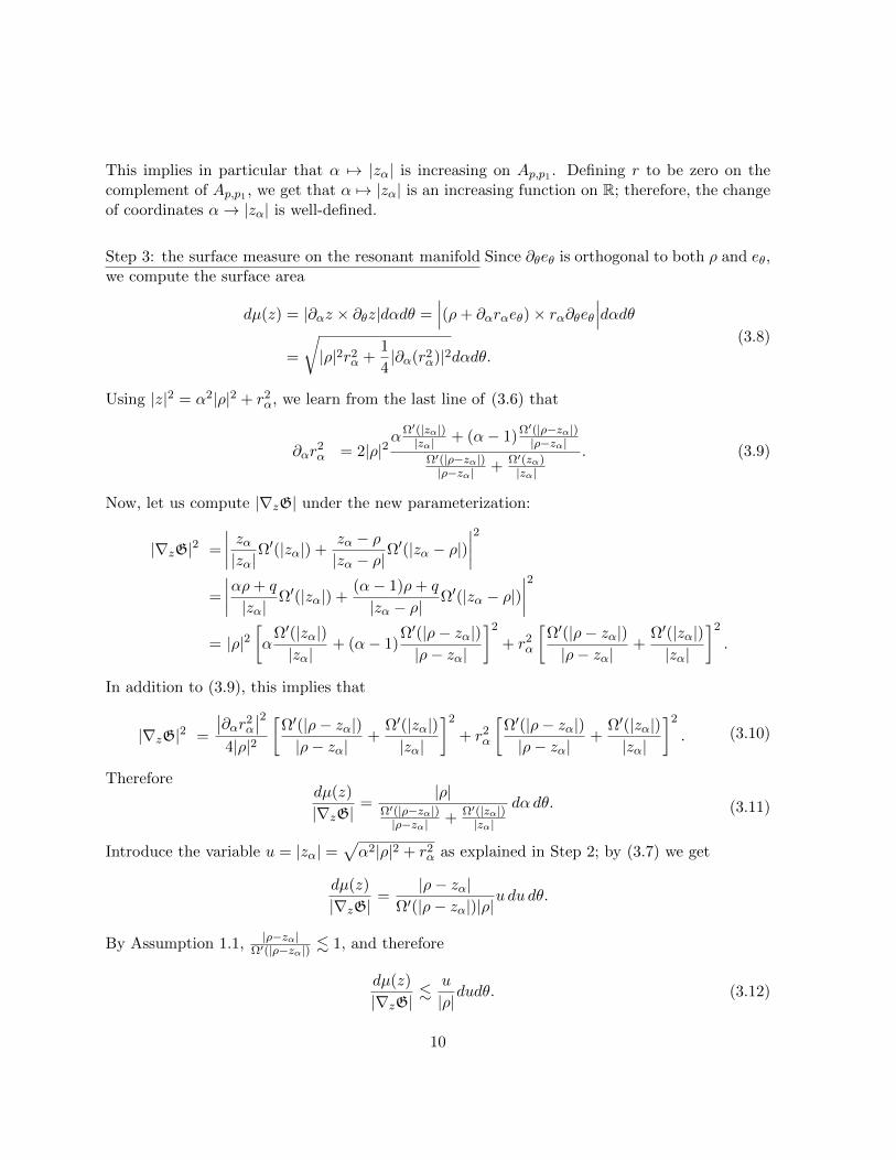
This implies in particular that α 7→ |zα| is increasing on Ap,p1 . Defining r to be zero on thecomplement of Ap,p1 , we get that α 7→ |zα| is an increasing function on R; therefore, the changeof coordinates α→ |zα| is well-defined.

Step 3: the surface measure on the resonant manifold Since ∂θeθ is orthogonal to both ρ and eθ,we compute the surface area

dµ(z) = |∂αz × ∂θz|dαdθ =∣∣∣(ρ+ ∂αrαeθ)× rα∂θeθ

∣∣∣dαdθ=

√|ρ|2r2

α +1

4|∂α(r2

α)|2dαdθ.(3.8)

Using |z|2 = α2|ρ|2 + r2α, we learn from the last line of (3.6) that

∂αr2α = 2|ρ|2

αΩ′(|zα|)|zα| + (α− 1)Ω′(|ρ−zα|)

|ρ−zα|Ω′(|ρ−zα|)|ρ−zα| + Ω′(zα)

|zα|

. (3.9)

Now, let us compute |∇zG| under the new parameterization:

|∇zG|2 =

∣∣∣∣ zα|zα|Ω′(|zα|) +zα − ρ|zα − ρ|

Ω′(|zα − ρ|)∣∣∣∣2

=

∣∣∣∣αρ+ q

|zα|Ω′(|zα|) +

(α− 1)ρ+ q

|zα − ρ|Ω′(|zα − ρ|)

∣∣∣∣2= |ρ|2

[α

Ω′(|zα|)|zα|

+ (α− 1)Ω′(|ρ− zα|)|ρ− zα|

]2

+ r2α

[Ω′(|ρ− zα|)|ρ− zα|

+Ω′(|zα|)|zα|

]2

.

In addition to (3.9), this implies that

|∇zG|2 =

∣∣∂αr2α

∣∣24|ρ|2

[Ω′(|ρ− zα|)|ρ− zα|

+Ω′(|zα|)|zα|

]2

+ r2α

[Ω′(|ρ− zα|)|ρ− zα|

+Ω′(|zα|)|zα|

]2

. (3.10)

Thereforedµ(z)

|∇zG|=

|ρ|Ω′(|ρ−zα|)|ρ−zα| + Ω′(|zα|)

|zα|

dα dθ. (3.11)

Introduce the variable u = |zα| =√α2|ρ|2 + r2

α as explained in Step 2; by (3.7) we get

dµ(z)

|∇zG|=

|ρ− zα|Ω′(|ρ− zα|)|ρ|

u du dθ.

By Assumption 1.1, |ρ−zα|Ω′(|ρ−zα|) . 1, and therefore

dµ(z)

|∇zG|.

u

|ρ|dudθ. (3.12)

10

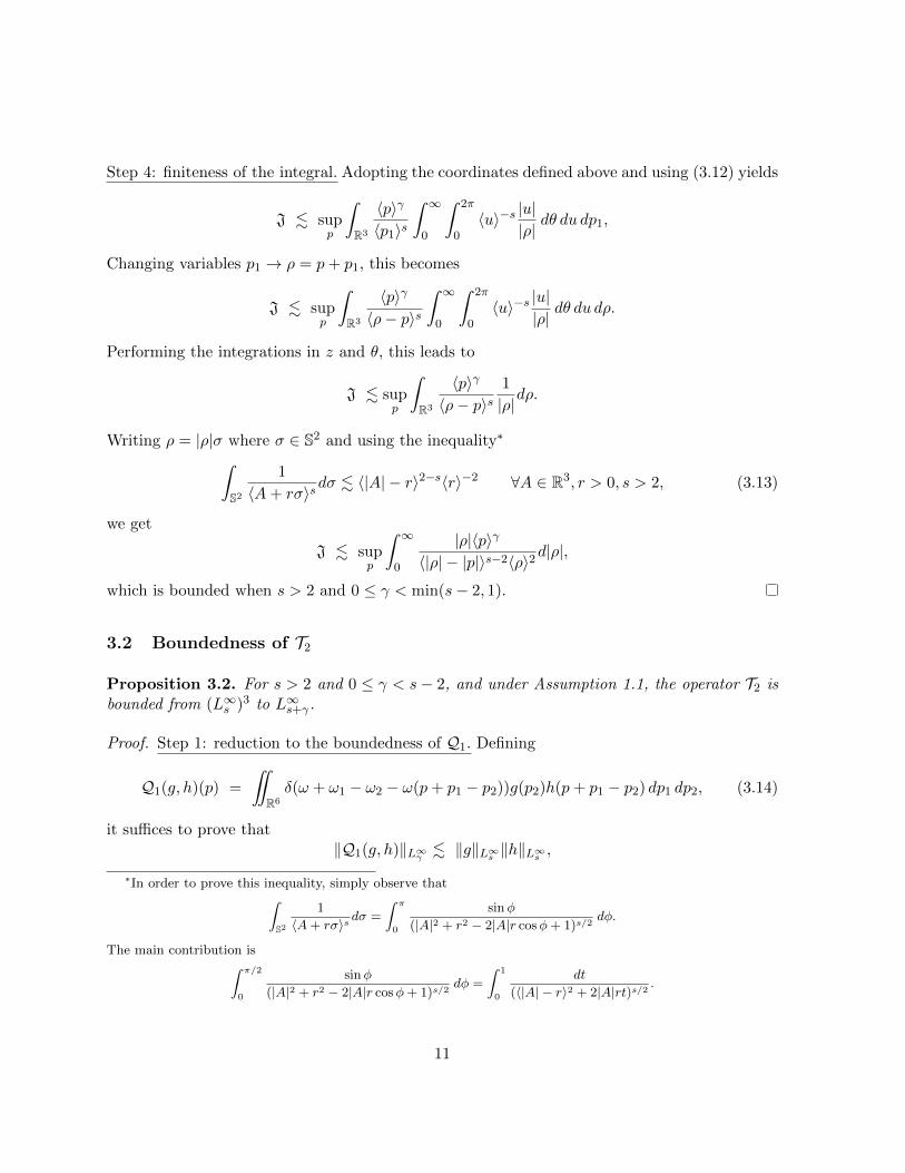
Step 4: finiteness of the integral. Adopting the coordinates defined above and using (3.12) yields

J . supp

ˆR3

〈p〉γ

〈p1〉s

ˆ ∞0

ˆ 2π

0〈u〉−s |u|

|ρ|dθ du dp1,

Changing variables p1 → ρ = p+ p1, this becomes

J . supp

ˆR3

〈p〉γ

〈ρ− p〉s

ˆ ∞0

ˆ 2π

0〈u〉−s |u|

|ρ|dθ du dρ.

Performing the integrations in z and θ, this leads to

J . supp

ˆR3

〈p〉γ

〈ρ− p〉s1

|ρ|dρ.

Writing ρ = |ρ|σ where σ ∈ S2 and using the inequality∗

ˆS2

1

〈A+ rσ〉sdσ . 〈|A| − r〉2−s〈r〉−2 ∀A ∈ R3, r > 0, s > 2, (3.13)

we get

J . supp

ˆ ∞0

|ρ|〈p〉γ

〈|ρ| − |p|〉s−2〈ρ〉2d|ρ|,

which is bounded when s > 2 and 0 ≤ γ < min(s− 2, 1).

3.2 Boundedness of T2

Proposition 3.2. For s > 2 and 0 ≤ γ < s− 2, and under Assumption 1.1, the operator T2 isbounded from (L∞s )3 to L∞s+γ.

Proof. Step 1: reduction to the boundedness of Q1. Defining

Q1(g, h)(p) =

¨R6

δ(ω + ω1 − ω2 − ω(p+ p1 − p2))g(p2)h(p+ p1 − p2) dp1 dp2, (3.14)

it suffices to prove that‖Q1(g, h)‖L∞γ . ‖g‖L∞s ‖h‖L∞s ,

∗In order to prove this inequality, simply observe thatˆS2

1

〈A+ rσ〉s dσ =

ˆ π

0

sinφ

(|A|2 + r2 − 2|A|r cosφ+ 1)s/2dφ.

The main contribution isˆ π/2

0

sinφ

(|A|2 + r2 − 2|A|r cosφ+ 1)s/2dφ =

ˆ 1

0

dt

(〈|A| − r〉2 + 2|A|rt)s/2.

11

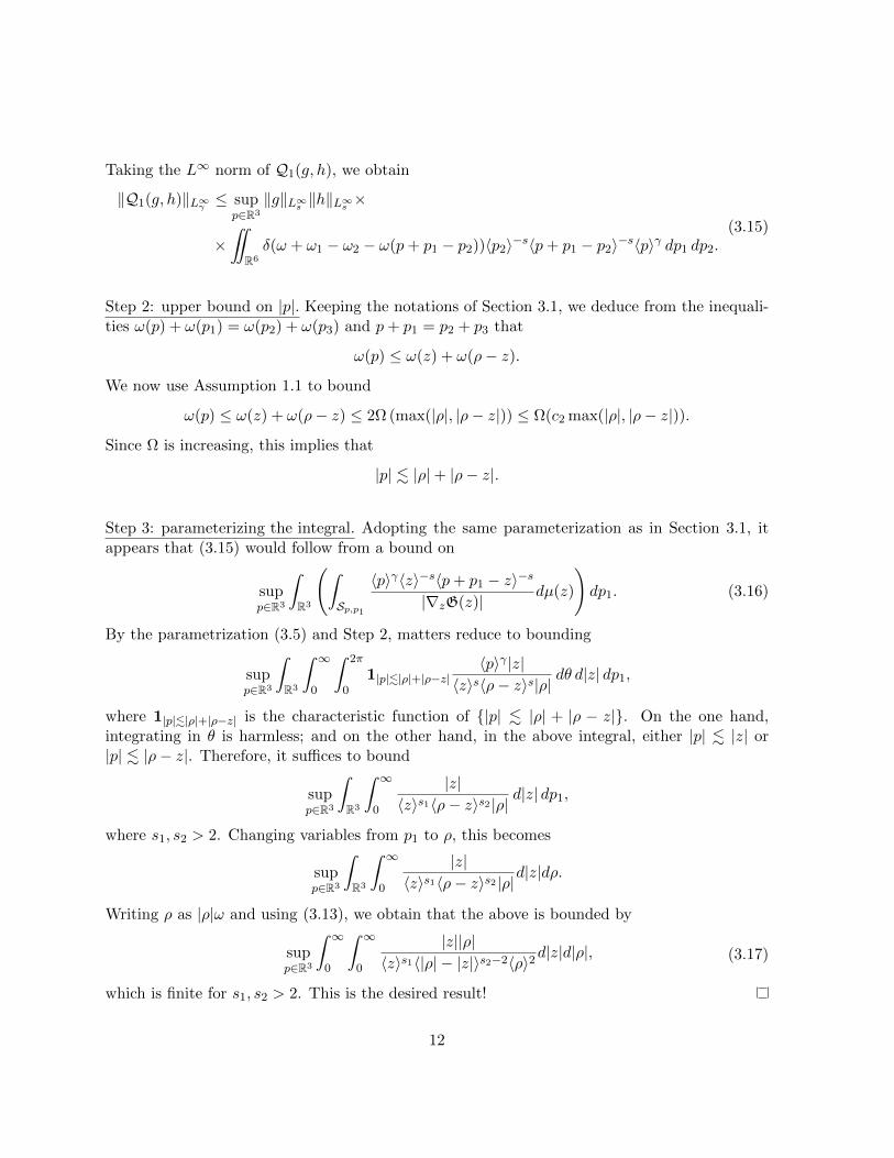
Taking the L∞ norm of Q1(g, h), we obtain

‖Q1(g, h)‖L∞γ ≤ supp∈R3

‖g‖L∞s ‖h‖L∞s ×

ר

R6

δ(ω + ω1 − ω2 − ω(p+ p1 − p2))〈p2〉−s〈p+ p1 − p2〉−s〈p〉γ dp1 dp2.(3.15)

Step 2: upper bound on |p|. Keeping the notations of Section 3.1, we deduce from the inequali-ties ω(p) + ω(p1) = ω(p2) + ω(p3) and p+ p1 = p2 + p3 that

ω(p) ≤ ω(z) + ω(ρ− z).

We now use Assumption 1.1 to bound

ω(p) ≤ ω(z) + ω(ρ− z) ≤ 2Ω (max(|ρ|, |ρ− z|)) ≤ Ω(c2 max(|ρ|, |ρ− z|)).

Since Ω is increasing, this implies that

|p| . |ρ|+ |ρ− z|.

Step 3: parameterizing the integral. Adopting the same parameterization as in Section 3.1, itappears that (3.15) would follow from a bound on

supp∈R3

ˆR3

(ˆSp,p1

〈p〉γ〈z〉−s〈p+ p1 − z〉−s

|∇zG(z)|dµ(z)

)dp1. (3.16)

By the parametrization (3.5) and Step 2, matters reduce to bounding

supp∈R3

ˆR3

ˆ ∞0

ˆ 2π

01|p|.|ρ|+|ρ−z|

〈p〉γ |z|〈z〉s〈ρ− z〉s|ρ|

dθ d|z| dp1,

where 1|p|.|ρ|+|ρ−z| is the characteristic function of |p| . |ρ| + |ρ − z|. On the one hand,integrating in θ is harmless; and on the other hand, in the above integral, either |p| . |z| or|p| . |ρ− z|. Therefore, it suffices to bound

supp∈R3

ˆR3

ˆ ∞0

|z|〈z〉s1〈ρ− z〉s2 |ρ|

d|z| dp1,

where s1, s2 > 2. Changing variables from p1 to ρ, this becomes

supp∈R3

ˆR3

ˆ ∞0

|z|〈z〉s1〈ρ− z〉s2 |ρ|

d|z|dρ.

Writing ρ as |ρ|ω and using (3.13), we obtain that the above is bounded by

supp∈R3

ˆ ∞0

ˆ ∞0

|z||ρ|〈z〉s1〈|ρ| − |z|〉s2−2〈ρ〉2

d|z|d|ρ|, (3.17)

which is finite for s1, s2 > 2. This is the desired result!

12

3.3 Boundedness of T3

Proposition 3.3. For s > 2 and 0 ≤ γ < min(s − 2, 1), and under Assumption 1.1, theoperator T3 is bounded from (L∞s )3 to L∞s+γ.

Proof. Defining

Q2(g, h) =

ˆR6

δ(ω(p) + ω(p1)− ω(p2)− ω(p+ p1 − p2))g(p1)h(p2) dp1 dp2, (3.18)

it suffices to show that‖Q2(g, h)‖L∞γ ≤ C‖g‖L∞s ‖h‖L∞s .

Similar as in section 3.2, we set ρ = p+ p1, and define G and Sp,p1 in exactly the same way with(3.3). As a result, Q2(g, h) can be recast under the following form.

Q2(g, h) =

ˆR3

g(p1)

(ˆSp,p1

h(z)

|∇G(z)|dz

)dp1. (3.19)

Proceeding as in the proof of Proposition 3.1, it suffices to prove the boundedness of

J = supp∈R3

(ˆR3

〈p1〉−s〈p〉γ(ˆ c2(|p|+|p1|)

0

ˆ 2π

0〈z〉−s |z|

|ρ|dθd|z|

)dp1

). (3.20)

The right hand side of (3.20) contains an integral with respect to p1, which can be switched intoan integral in ρ by the change of variable p1 → ρ, in the following way

J . supp∈R3

(ˆR3

〈ρ− p〉−s〈p〉γ(ˆ c2(|p|+|ρ−p|)

0

ˆ 2π

0〈z〉−s |z|

|ρ|dθd|z|

)dρ

)

. supp∈R3

(ˆR3

ˆ ∞0〈ρ− p〉−s〈p〉γ〈z〉−s |z|

|ρ|d|z|dρ

). sup

p∈R3

(ˆR3

〈ρ− p〉−s〈p〉γ 1

|ρ|dρ

),

(3.21)

where the last inequality is due to the fact that s > 2.

Writing ρ as |ρ|ω and using (3.13), we obtain

J . supp∈R3

(ˆR3

〈ρ− p〉−s〈p〉γ 1

|ρ|dρ

). sup

p∈R3

(ˆ ∞0

〈p〉γ |ρ|〈ρ〉2〈|ρ| − |p|〉s−2

d|ρ|).

(3.22)

which is bounded when s > 2 and 0 ≤ γ < min(2− s, 1).

13

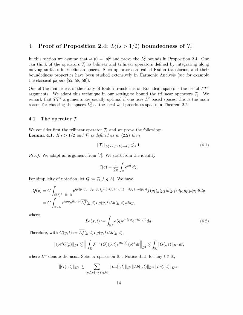
4 Proof of Proposition 2.4: L2s(s > 1/2) boundedness of Tj

In this section we assume that ω(p) = |p|2 and prove the L2s bounds in Proposition 2.4. One

can think of the operators Tj as bilinear and trilinear operators defined by integrating alongmoving surfaces in Euclidean spaces. Such operators are called Radon transforms, and theirboundedness properties have been studied extensively in Harmonic Analysis (see for examplethe classical papers [55, 58, 59]).

One of the main ideas in the study of Radon transforms on Euclidean spaces is the use of TT ∗

arguments. We adapt this technique in our setting to bound the trilinear operators Tj . Weremark that TT ∗ arguments are usually optimal if one uses L2 based spaces; this is the mainreason for choosing the spaces L2

s as the local well-posedness spaces in Theorem 2.2.

4.1 The operator T1

We consider first the trilinear operator T1 and we prove the following:Lemma 4.1. If s > 1/2 and T1 is defined as in (2.2) then

‖T1‖L2s×L2

s×L2s→L2

s.s 1. (4.1)

Proof. We adapt an argument from [7]. We start from the identity

δ(q) =1

2π

ˆReiqξ dξ.

For simplicity of notation, let Q := T1[f, g, h]. We have

Q(p) = C

ˆ(Rd)3×R×R

eiy·(p+p1−p2−p3)eit(ω(p)+ω(p1)−ω(p2)−ω(p3))f(p1)g(p2)h(p3) dp1dp2dp3dtdy

= C

ˆR×R

eiy·peitω(p)Lf(y, t)Lg(y, t)Lh(y, t) dtdy,

where

La(x, t) :=

ˆRda(q)e−iq·xe−iω(q)t dq. (4.2)

Therefore, with G(y, t) := Lf(y, t)Lg(y, t)Lh(y, t),

‖〈p〉sQ(p)‖L2 .∥∥∥ˆ

RF−1(G)(p, t)eitω(p)〈p〉s dt

∥∥∥L2

.ˆR‖G(., t)‖Hs dt,

where Hs denote the usual Sobolev spaces on R3. Notice that, for any t ∈ R,

‖G(., t)‖Hs .∑

a,b,c=f,g,h

‖La(., t)‖Hs‖Lb(., t)‖L∞‖Lc(., t)‖L∞ .

14

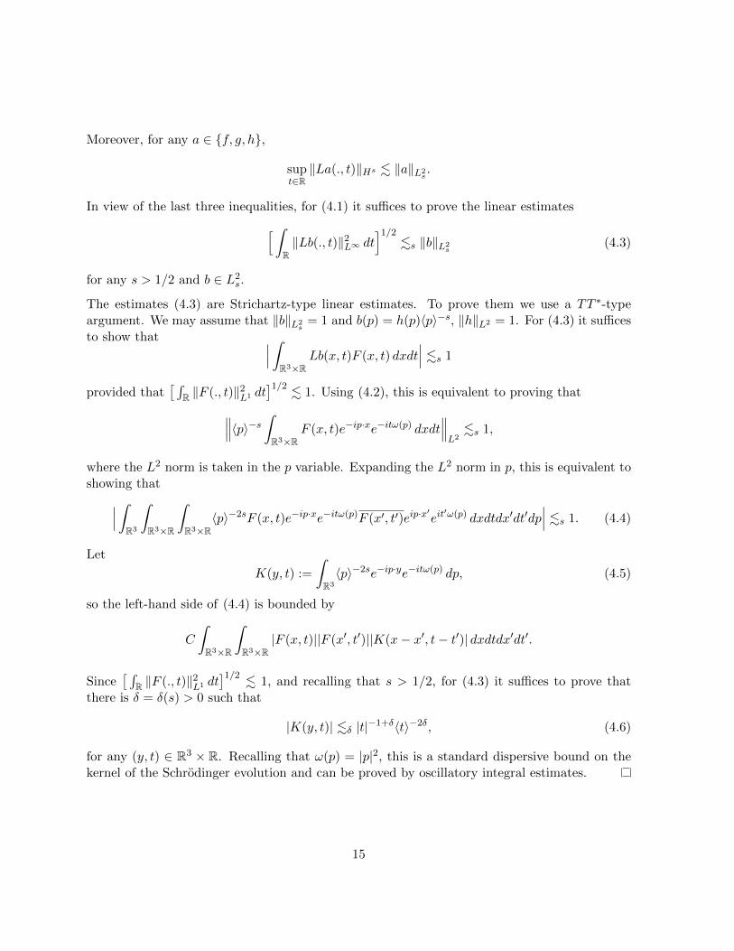
Moreover, for any a ∈ f, g, h,

supt∈R‖La(., t)‖Hs . ‖a‖L2

s.

In view of the last three inequalities, for (4.1) it suffices to prove the linear estimates[ ˆR‖Lb(., t)‖2L∞ dt

]1/2.s ‖b‖L2

s(4.3)

for any s > 1/2 and b ∈ L2s.

The estimates (4.3) are Strichartz-type linear estimates. To prove them we use a TT ∗-typeargument. We may assume that ‖b‖L2

s= 1 and b(p) = h(p)〈p〉−s, ‖h‖L2 = 1. For (4.3) it suffices

to show that ∣∣∣ ˆR3×R

Lb(x, t)F (x, t) dxdt∣∣∣ .s 1

provided that[ ´

R ‖F (., t)‖2L1 dt]1/2

. 1. Using (4.2), this is equivalent to proving that∥∥∥〈p〉−s ˆR3×R

F (x, t)e−ip·xe−itω(p) dxdt∥∥∥L2

.s 1,

where the L2 norm is taken in the p variable. Expanding the L2 norm in p, this is equivalent toshowing that∣∣∣ ˆ

R3

ˆR3×R

ˆR3×R

〈p〉−2sF (x, t)e−ip·xe−itω(p)F (x′, t′)eip·x′eit′ω(p) dxdtdx′dt′dp

∣∣∣ .s 1. (4.4)

Let

K(y, t) :=

ˆR3

〈p〉−2se−ip·ye−itω(p) dp, (4.5)

so the left-hand side of (4.4) is bounded by

C

ˆR3×R

ˆR3×R

|F (x, t)||F (x′, t′)||K(x− x′, t− t′)| dxdtdx′dt′.

Since[ ´

R ‖F (., t)‖2L1 dt]1/2

. 1, and recalling that s > 1/2, for (4.3) it suffices to prove thatthere is δ = δ(s) > 0 such that

|K(y, t)| .δ |t|−1+δ〈t〉−2δ, (4.6)

for any (y, t) ∈ R3 × R. Recalling that ω(p) = |p|2, this is a standard dispersive bound on thekernel of the Schrodinger evolution and can be proved by oscillatory integral estimates.

15

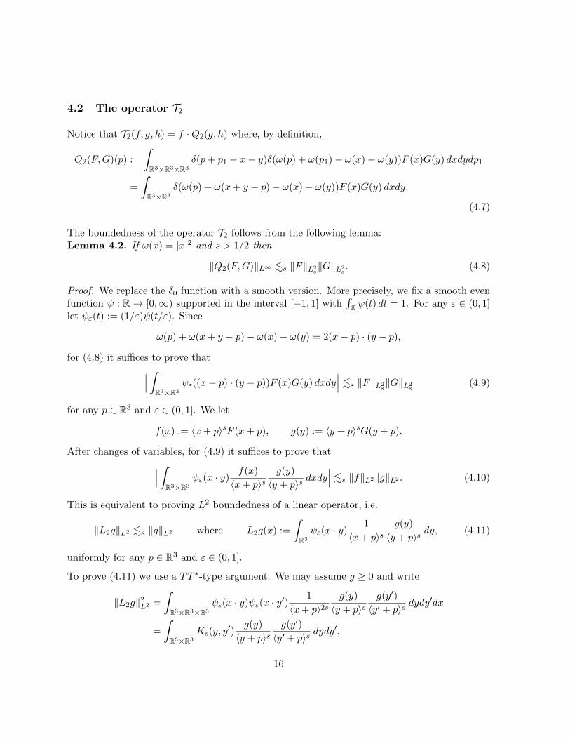
4.2 The operator T2

Notice that T2(f, g, h) = f ·Q2(g, h) where, by definition,

Q2(F,G)(p) :=

ˆR3×R3×R3

δ(p+ p1 − x− y)δ(ω(p) + ω(p1)− ω(x)− ω(y))F (x)G(y) dxdydp1

=

ˆR3×R3

δ(ω(p) + ω(x+ y − p)− ω(x)− ω(y))F (x)G(y) dxdy.

(4.7)

The boundedness of the operator T2 follows from the following lemma:Lemma 4.2. If ω(x) = |x|2 and s > 1/2 then

‖Q2(F,G)‖L∞ .s ‖F‖L2s‖G‖L2

s. (4.8)

Proof. We replace the δ0 function with a smooth version. More precisely, we fix a smooth evenfunction ψ : R→ [0,∞) supported in the interval [−1, 1] with

´R ψ(t) dt = 1. For any ε ∈ (0, 1]

let ψε(t) := (1/ε)ψ(t/ε). Since

ω(p) + ω(x+ y − p)− ω(x)− ω(y) = 2(x− p) · (y − p),

for (4.8) it suffices to prove that∣∣∣ˆR3×R3

ψε((x− p) · (y − p))F (x)G(y) dxdy∣∣∣ .s ‖F‖L2

s‖G‖L2

s(4.9)

for any p ∈ R3 and ε ∈ (0, 1]. We let

f(x) := 〈x+ p〉sF (x+ p), g(y) := 〈y + p〉sG(y + p).

After changes of variables, for (4.9) it suffices to prove that∣∣∣ˆR3×R3

ψε(x · y)f(x)

〈x+ p〉sg(y)

〈y + p〉sdxdy

∣∣∣ .s ‖f‖L2‖g‖L2 . (4.10)

This is equivalent to proving L2 boundedness of a linear operator, i.e.

‖L2g‖L2 .s ‖g‖L2 where L2g(x) :=

ˆR3

ψε(x · y)1

〈x+ p〉sg(y)

〈y + p〉sdy, (4.11)

uniformly for any p ∈ R3 and ε ∈ (0, 1].

To prove (4.11) we use a TT ∗-type argument. We may assume g ≥ 0 and write

‖L2g‖2L2 =

ˆR3×R3×R3

ψε(x · y)ψε(x · y′)1

〈x+ p〉2sg(y)

〈y + p〉sg(y′)

〈y′ + p〉sdydy′dx

=

ˆR3×R3

Ks(y, y′)

g(y)

〈y + p〉sg(y′)

〈y′ + p〉sdydy′,

16

where

Ks(y, y′) = Ks,ε,p(y, y

′) :=

ˆR3

ψε(x · y)ψε(x · y′)1

〈x+ p〉2sdx.

Using Lemma 4.3 (ii) below, we have

|Ks(y, y′)| .s

1

|y||y′|

( 1

|y − y′|+

1

|y + y′|

),

where x := x/|x| for any x ∈ R3. For (4.11) it suffices to prove that∣∣∣ ˆR3×R3

1

|y||y′|1

|y − y′|· g(y)

〈y + p〉sh(y′)

〈y′ + p′〉sdydy′

∣∣∣ .s ‖g‖L2‖h‖L2 , (4.12)

for any g, h ∈ L2(R3) and any p, p′ ∈ R3.

For θ, θ′ ∈ S2 let

g(θ) :=[ˆ ∞

0|g(rθ)|2r2 dr

]1/2, h(θ′) :=

[ˆ ∞0|h(rθ′)|2r2 dr

]1/2.

We make the changes of variables y = rθ and y′ = r′θ′ in the integral in the left-hand side of(4.12). Notice that

ˆ ∞0

g(rθ)

〈rθ + p〉sr dr .s g(θ),

ˆ ∞0

h(r′θ′)

〈r′θ′ + p′〉sr′ dr′ .s h(θ′),

using the Cauchy-Schwarz inequality and (4.13). Thus the integral in the left-hand side of (4.12)is bounded by

Cs

∣∣∣ ˆS2×S2

1

|θ − θ′|· g(θ)h(θ′) dθdθ′

∣∣∣.Using Schur’s lemma this is bounded by ‖g‖L2(S2)‖h‖L2(S2), and the desired estimates (4.12)follow. This completes the proof.

We summarize below two technical estimates we used in the proof of Lemma 4.2.Lemma 4.3. (i) If θ ∈ S2 and p ∈ R then

ˆR

1

〈rθ + p〉2sdr .s 1. (4.13)

(ii) Assume that ε1, ε2 ∈ [0, 1), a, b ∈ R, p ∈ R3, u, v ∈ S2, and s > 1/2. Then

ˆR3

1[0,ε1](x · v − a)1[0,ε2](x · w − b)1

〈x+ p〉2sdx .s

ε1ε2

|v − w|+

ε1ε2

|v + w|. (4.14)

17

Proof. (i) By rotation invariance, we may assume ω = (1, 0, 0). The bound (4.13) is then impliedby the easy estimate

supq1,q2,q3∈R

ˆR

1[(r + q1)2 + q2

2 + q23 + 1

]s dr .s 1. (4.15)

(ii) We may assume ε1 ≤ ε2. By rotation invariance, we may assume v = (1, 0, 0) and w =(w1, w2, 0). Clearly, |w2| ≈ min(|v − w|, |v + w|). Notice also that

x · w − b = x1w1 + x2w2 − b = x2w2 − (b− aw1) + (x1 − a)w1.

Since |w1| ≤ 1, the integral in the left-hand side of (4.14) is bounded byˆR3

1[0,ε1](x1 − a)1[−4ε2,4ε2](x2w2 − b′)1

〈x+ p〉2sdx.

The desired conclusion follows using (4.15) and integrating first the variable x3.

4.3 The operator T3

As in the previous subsection we notice that T3(f, g, h) = f ·Q3(g, h) where

Q3(F,G)(p) :=

ˆR3×R3×R3

δ(p− p3 + x− y)δ(ω(p)− ω(p3) + ω(x)− ω(y))F (x)G(y) dxdydp3

=

ˆR3×R3

δ(ω(p)− ω(x− y + p) + ω(x)− ω(y))F (x)G(y) dxdy.

(4.16)

In view of the definitions, boundedness of T3 follows from the following lemma:Lemma 4.4. If ω(x) = |x|2 as before and s > 1/2 then

‖Q3(F,G)‖L∞ .s ‖F‖L2s‖G‖L2

s. (4.17)

Proof. As before we replace δ with ψε and notice that

ω(p)− ω(x− y + p) + ω(x)− ω(y) = 2(x− y) · (y − p).

We let f(x) = 〈x+ p〉sF (x+ p) and g(y) = 〈y+ p〉sG(y+ p) as in the proof of Lemma 4.2. Afterchanges of variables, for (4.17) it suffices to prove that

‖L3g‖L2 .s ‖g‖L2 where L3g(x) :=

ˆR3

ψε((x− y) · y)1

〈x+ p〉sg(y)

〈y + p〉sdy, (4.18)

uniformly for p ∈ R3 and ε ∈ (0, 1]. This follows using the TT ∗ argument as in Proposition 4.2,the uniform bounds in Lemma 4.3 (ii), and (4.12).

18

5 Proof of Theorems 2.1 and 2.2

The two theorems follow by similar arguments from Propositions 2.3 and 2.4. For concreteness,we provide all the details only for the proof of Theorem 2.2.

Proof of Theorem 2.2. (i) Let T := A−1s R−2 for a sufficiently large constant As. We define the

approximating sequence

f0(t) := f0, fn+1(t) := f0 +

ˆ t

0Q(fn(τ)) dτ, (5.1)

on the interval [0, T ]. Using Proposition 2.4 it follows easily, by induction that fn ∈ C1([0, T ] :L2s) and supt∈[0,T ] ‖fn(t)‖L2

s≤ 2R. Using again Proposition 2.4 it follows that the sequence fn is

Cauchy in C([0, T ] : L2s), thus convergent to a function f ∈ C([0, T ] : L2

s) that has the properties

f(0) = f0, f(t) = f0 +

ˆ t

0Q[f(τ)] dτ, sup

t∈[0,T ]‖f(t)‖L2

s≤ 2R. (5.2)

In particular ∂tf = Q[f ], thus f ∈ C1([0, T ] : L2s). Uniqueness and continuity of the flow map

f0 → f follow again from the contraction principle.

(ii) Clearly, f is real-valued if f0 is real-valued. To prove non-negativity, we need to be slightlymore careful because the simple recursive scheme (5.1) does not preserve non-negativity.

Step 1: We construct a different approximating sequence, based on the temporal forward Euler

scheme: for any n ∈ N we set ∆n = T/n and define the sequence gn,mn−1i=0 by

gn,0 := f0, gn,m+1 := gn,m + ∆nQ[gn,m]. (5.3)

Then we define gn for t ∈ [m∆n, (m+ 1)∆n] by the formula

gn(t) := gn,m + (t−m∆n)Q[gn,m]

=1

∆n

((t−m∆n)gn,m+1 + ((m+ 1)∆n − t)gn,m

).

(5.4)

Using Proposition 2.4 inductively and the assumption T = A−1s R−2, it is easy to verify that

‖gn,m‖L2s≤ 2R for any n ≥ 1 and m ∈ 0, . . . , n− 1. (5.5)

In particular, using the definition (5.4),

gn ∈ C([0, T ] : L2s) for any n ≥ 1 and sup

t∈[0,T ]‖gn(t)‖L2

s≤ 2R. (5.6)

Step 2: We show now that

limn→∞

gn = f in C([0, T ] : L2s). (5.7)

19

Let δn := supt∈[0,T ] ‖gn(t) − f(t)‖L2s. Given t ∈ [0, T ] we fix m ∈ 0, 1, . . . , n − 1 such that

mT/n ≤ t ≤ (m+ 1)T/n. Then we write, using (5.2)–(5.4),

gn(t)− f(t)

= gn(t)− gn,m+gn,m − f0 −

ˆ mT/n

0Q[f(τ)] dτ

−ˆ t

mT/nQ[f(τ)] dτ

= I(t) + II(t) + III(t),

(5.8)

where

I(t) := (t−mT/n)Q[gn,m],

II(t) :=

m−1∑j=0

ˆ (j+1)T/n

jT/n

Q[gn,j ]−Q[f(τ)]

dτ,

III(t) := −ˆ t

mT/nQ[f(τ)] dτ.

Using Proposition 2.4 and the bounds (5.2) and (5.5) we estimate

‖I(t)‖L2s

+ ‖III(t)‖L2s. (T/n)R3 . R/n. (5.9)

We estimate also, for any τ ∈ [jT/n, (j + 1)T/n],∥∥Q[gn,j ]−Q[f(τ)]∥∥L2s.∥∥Q[gn,j ]−Q[gn(τ)]

∥∥L2s

+∥∥Q[gn(τ)]−Q[f(τ)]

∥∥L2s

. (T/n)R5 + δnR2,

using Proposition 2.4 and recalling the definition δn := supt∈[0,T ] ‖gn(t)− f(t)‖L2s. Thus

‖II(t)‖L2s. R/n+ δn(TR2). (5.10)

Since TR2 ≤ A−1s 1, it follows from (5.8)–(5.10) that δn . R/n. The desired conclusion (5.7)

follows.

Step 3: Finally, we show that all the functions gn are non-negative. In view of the defintion (5.4),it suffices to prove that the functions gn,m are non-negative for any n ≥ 1 and m ∈ 0, . . . , n−1.We prove this by induction over m. The case m = 0 follows from the hypothesis f0 ≥ 0.Moreover, recalling the definition (2.1),

gn,m+1 ≥ gn,m + ∆n

[T2(gn,m, gn,m, gn,m) + T3(gn,m, gn,m, gn,m)

].

Recall that Tk(gn,m, gn,m, gn,m) = gn,m · Qk(gn,m, gn,m), k ∈ 1, 2, see definitions (4.7) and(4.16). Using Lemmas 4.2 and 4.4, it follows that

gn,m+1 ≥ (1− CsR2T/n)gn,m ≥ (1− 1/(2n))gn,m.

The non-negativity of the functions gn,m follows. This implies the non-negativity of the solutionf , as a consequence of (5.7).

20

6 Further results

Define the function space Lrs by the norm

‖f‖Lrs = ‖(1 + ωp)sf‖Lr .

Notice that our theorems 2.1 and 2.2 are valid for the case where the initial condition does notbelong to L1

1. In this case, moment estimate techniques, such as those used in [6, 2] are notapplicable.

Now, if we consider the 4-wave turbulence kinetic equation (1.1) (or (2.1)), and suppose inaddition that f0 ∈ L1

1; similar to the case of the classical Boltzmann equation [61], we also havethe conservation of mass, momentum and energy of solutions to (1.1).

Taking any ϕ ∈ Cc(R3) as a test function in (1.1), the following weak formulation holdstrue ˆ

R3

Q[f ]ϕdp =

ˆR9

δ(p+ p1 − p2 − p3)δ(ω + ω1 − ω2 − ω3)×

× ff1(f2 + f3)[ϕ2 + ϕ3 − ϕ− ϕ1]dp1dp2dp3dp,

(6.1)

in which, again, we have used the abbreviation ϕ = ϕ(t, p), ϕ1 = ϕ(t, p1), ϕ2 = ϕ(t, p2),ϕ3 = ϕ(t, p3). By choosing ϕ to be 1, p or ω, the right hand side of (6.1) vanishes.

Since

∂t

ˆR3

fϕdp =

ˆR3

Q[f ]ϕdp,

the following conservation laws are then satisfied

∂t

ˆR3

fdp = ∂t

ˆR3

fpidp = ∂t

ˆR3

fωdp = 0, (6.2)

with p = (p1, p2, p3), i ∈ 1, 2, 3, or equivalently

ˆR3

f(t, p)dp =

ˆR3

f0(p)dp,

ˆR3

f(t, p)pidp =

ˆR3

f0(p)pidp,

ˆR3

f(t, p)ωpdp =

ˆR3

f0(p)ωpdp.

(6.3)

By the same argument used in (ii) of the proofs of Theorem 2.1 and Theorem 2.2, we obtain thefollowing theorem.

21

Theorem 6.1. Assume that ω and the positive initial condition f0 satisfy the assumptions ofTheorem 2.1 and Theorem 2.2. In addition, suppose f0 ∈ L1

1. Then the same conclusion ofTheorem 2.1 and Theorem 2.2 holds true. Furthermore, f ∈ C([0, T ] : L1

1) and f also satisfiesthe conservation laws (6.3).

Acknowledgment: PG was supported by the National Science Foundation grant DMS-1301380.ADI was supported in part by NSF grant DMS-1600028 and by NSF-FRG grant DMS-1463753.MBT was supported by NSF Grant DMS (Ki-Net) 1107291, ERC Advanced Grant DYCON.The authors would like to thank Sergey Nazarenko and Alan Newell for fruitful discussions onthe topic.

References

[1] R. Alonso, J. A. Canizo, I. M. Gamba, and Clement Mouhot. A new approach to thecreation and propagation of exponential moments in the Boltzmann equation. Comm.Partial Differential Equations, 38(1):155–169, 2013.

[2] R. Alonso, I. M. Gamba, and M.-B. Tran. Propagation of moments of the quantum Boltz-mann equation at very low temperature. Submitted.

[3] L. Arkeryd and A. Nouri. On the cauchy problem with large data for a space-dependentboltzmann-nordheim boson equation. arXiv preprint arXiv:1601.06927, 2016.

[4] A. V. Bobylev and I. M. Gamba. Boltzmann equations for mixtures of Maxwell gases: exactsolutions and power like tails. J. Stat. Phys., 124(2-4):497–516, 2006.

[5] D. Bohm and D. Pines. A collective description of electron interactions. i. magnetic inter-actions. Physical Review, 82(5):625, 1951.

[6] M. Briant and A. Einav. On the Cauchy problem for the homogeneous Boltzmann-Nordheimequation for bosons: local existence, uniqueness and creation of moments. J. Stat. Phys.,163(5):1108–1156, 2016.

[7] T. Buckmaster, P. Germain, Z. Hani, and J. Shatah. Analysis of the (CR) equation inhigher dimensions. International Mathematics Research Notices Accepted, 2017.

[8] T. Buckmaster, P. Germain, Z. Hani, and J. Shatah. Effective dynamics of the nonlinearschrodinger equation on large domains. Communications on Pure and Applied MathematicsAccepted, 2017.

[9] Torsten Carleman. Sur la theorie de l’equation integrodifferentielle de Boltzmann. ActaMath., 60(1):91–146, 1933.

[10] Carlo Cercignani. The Boltzmann equation and its applications, volume 67 of AppliedMathematical Sciences. Springer-Verlag, New York, 1988.

22

[11] G. Craciun and M.-B. Tran. A toric dynamical system approach to the convergence toequilibrium of quantum Boltzmann equations for bose gases. Submitted.

[12] A. I. Dyachenko and V. E. Zakharov. Is free-surface hydrodynamics an integrable system?Physics Letters A, 190(2):144–148, 1994.

[13] S. Dyachenko, A. C. Newell, A. Pushkarev, and V. E. Zakharov. Optical turbulence: weakturbulence, condensates and collapsing filaments in the nonlinear Schrodinger equation.Phys. D, 57(1-2):96–160, 1992.

[14] U. Eckern. Relaxation processes in a condensed bose gas. J. Low Temp. Phys., 54:333–359,1984.

[15] M. Escobedo, F. Pezzotti, and M. Valle. Analytical approach to relaxation dynamics ofcondensed Bose gases. Ann. Physics, 326(4):808–827, 2011.

[16] M. Escobedo and M.-B. Tran. Convergence to equilibrium of a linearized quantum Boltz-mann equation for bosons at very low temperature. Kinetic and Related Models, 8(3):493—531, 2015.

[17] M. Escobedo and J. J. L. Velazquez. Finite time blow-up and condensation for the bosonicNordheim equation. Invent. Math., 200(3):761–847, 2015.

[18] M. Escobedo and J. J. L. Velazquez. On the theory of weak turbulence for the nonlinearSchrodinger equation. Mem. Amer. Math. Soc., 238(1124):v+107, 2015.

[19] E. Faou, P. Germain, and Z. Hani. The weakly nonlinear large-box limit of the 2d cubicnonlinear schr’odinger equation. Journal of the American Mathematical Society, 29(4):915–982, 2016.

[20] N. Fitzmaurice. Nonlinear waves and weak turbulence with applications in oceanographyand condensed matter physics, volume 11. Birkhauser, 1993.

[21] I. M. Gamba, V. Panferov, and C. Villani. On the Boltzmann equation for diffusivelyexcited granular media. Comm. Math. Phys., 246(3):503–541, 2004.

[22] I. M. Gamba, V. Panferov, and C. Villani. Upper Maxwellian bounds for the spatiallyhomogeneous Boltzmann equation. Arch. Ration. Mech. Anal., 194(1):253–282, 2009.

[23] I. M. Gamba, L. M. Smith, and M.-B. Tran. On the wave turbulence theory for stratifiedflows in the ocean. arXiv preprint arXiv:1709.08266, 2017.

[24] P. Germain, Z. Hani, and L. Thomann. On the continuous resonant equation for NLS, II:Statistical study. Analysis & PDE, 8(7):1733–1756, 2015.

[25] P. Germain, Z. Hani, and L. Thomann. On the continuous resonant equation for NLS.I. Deterministic analysis. Journal de Mathematiques Pures et Appliquees, 105(1):131–163,2016.

23

[26] K. Hasselmann. On the non-linear energy transfer in a gravity-wave spectrum. I. Generaltheory. J. Fluid Mech., 12:481–500, 1962.

[27] K. Hasselmann. On the non-linear energy transfer in a gravity wave spectrum. II. Conser-vation theorems; wave-particle analogy; irreversibility. J. Fluid Mech., 15:273–281, 1963.

[28] K Hasselmann. Feynman diagrams and interaction rules of wave-wave scattering processes.Reviews of Geophysics, 4(1):1–32, 1966.

[29] M. Imamovic-Tomasovic and A. Griffin. Quasiparticle kinetic equation in a trapped bosegas at low temperatures. J. Low Temp. Phys., 122:617–655, 2001.

[30] S. Jin and M.-B. Tran. Quantum hydrodynamic approximations to the finite temperaturetrapped Bose gases. Submitted.

[31] A. H. M. Kierkels and J. J. L. Velazquez. On self-similar solutions to a kinetic equationarising in weak turbulence theory for the Nonlinear Schrodinger Equation. arXiv preprintarXiv:1511.01292, 2015.

[32] A. H. M. Kierkels and J. J. L. Velazquez. On the transfer of energy towards infinity in thetheory of weak turbulence for the Nonlinear Schrodinger Equation. Journal of StatisticalPhysics, 3(159):668–712, 2015.

[33] G. V. Kolmakov, P. V. E. McClintock, and S. V. Nazarenko. Wave turbulence in quantumfluids. Proceedings of the National Academy of Sciences, 111(Supplement 1):4727–4734,2014.

[34] R. Lacaze, P. Lallemand, Y. Pomeau, and S. Rica. Dynamical formation of a Bose-Einsteincondensate. Phys. D, 152/153:779–786, 2001. Advances in nonlinear mathematics andscience.

[35] W. Li and X. Lu. The global existence of solutions of the boltzmann equation for bose-einstein particles with anisotropic initial data. arXiv preprint arXiv:1706.06235, 2017.

[36] X. Lu. On isotropic distributional solutions to the Boltzmann equation for Bose-Einsteinparticles. J. Statist. Phys., 116(5-6):1597–1649, 2004.

[37] X. Lu. The Boltzmann equation for Bose-Einstein particles: velocity concentration andconvergence to equilibrium. J. Stat. Phys., 119(5-6):1027–1067, 2005.

[38] X. Lu. The Boltzmann equation for Bose-Einstein particles: condensation in finite time. J.Stat. Phys., 150(6):1138–1176, 2013.

[39] J. Lukkarinen and H. Spohn. Weakly nonlinear Schrodinger equation with random initialdata. Invent. Math., 183(1):79–188, 2011.

[40] Y. V. Lvov, R. Binder, and A. C. Newell. Quantum weak turbulence with applications tosemiconductor lasers. Physica D: Nonlinear Phenomena, 121(3):317–343, 1998.

24

[41] Y. V. Lvov and A. C. Newell. Finite flux solutions of the quantum boltzmann equation andsemiconductor lasers. Physical review letters, 84(9):1894, 2000.

[42] S. Merino-Aceituno. Isotropic wave turbulence with simplified kernels: Existence, unique-ness, and mean-field limit for a class of instantaneous coagulation-fragmentation processes.Journal of Mathematical Physics, 57(12):121501, 2016.

[43] Sergey Nazarenko. Wave turbulence, volume 825 of Lecture Notes in Physics. Springer,Heidelberg, 2011.

[44] A. C. Newell and B. Rumpf. Wave turbulence. Annual review of fluid mechanics, 43:59–78,2011.

[45] A. C. Newell and B. Rumpf. Wave turbulence: A story far from over. World ScientificSeries on Nonlinear Science Series A, 83, 2013.

[46] C. S. Ng and A. Bhattacharjee. Interaction of shear-alfven wave packets: implicationfor weak magnetohydrodynamic turbulence in astrophysical plasmas. The AstrophysicalJournal, 465:845, 1996.

[47] T. Nguyen and M.-B. Tran. Uniform in time lower bound for solutions to a quantumBoltzmann equation of bosons at low temperatures. submitted.

[48] T. Nguyen and M.-B. Tran. On a quantum boltzmann type equation in zakharov’s waveturbulence theory. arXiv preprint arXiv:1702.03892, 2017.

[49] L.W. Nordheim. On the kinetic methods in the new statistics and its applications in theelectron theory of conductivity. Proc. Roy. Soc. London Ser. A, 119:689–698, 1928.

[50] S. Osher and R. Fedkiw. Level set methods and dynamic implicit surfaces, volume 153 ofApplied Mathematical Sciences. Springer-Verlag, New York, 2003.

[51] R. Peierls. Zur kinetischen theorie der warmeleitung in kristallen. Annalen der Physik,395(8):1055–1101, 1929.

[52] R. E. Peierls. Quantum theory of solids. In Theoretical physics in the twentieth century(Pauli memorial volume), pages 140–160. Interscience, New York, 1960.

[53] L. E. Reichl and M.-B. Tran. A kinetic model for very low temperature dilute bose gases.arXiv preprint arXiv:1709.09982, 2017.

[54] L. Saint-Raymond. Kinetic models for superfluids: a review of mathematical results.Comptes Rendus Physique, 5(1):65–75, 2004.

[55] A. Seeger. Radon transforms and finite type conditions. J. Amer. Math. Soc., 11(4):869–897, 1998.

[56] A. Soffer and M.-B. Tran. On coupling kinetic and schrodinger equations. Submitted.

25

[57] A. Soffer and M.-B. Tran. On the dynamics of finite temperature trapped bose gases.Submitted.

[58] C. D. Sogge and E. M. Stein. Averages of functions over hypersurfaces in Rn. Inventionesmathematicae, 82(3):543–556, 1985.

[59] C. D. Sogge and E. M. Stein. Averages over hypersurfaces. Smoothness of generalizedRadon transforms. J. Analyse Math., 54:165–188, 1990.

[60] E.A. Uehling and G.E. Uhlenbeck. Transport phenomena in einstein-bose and fermi-diracgases. Phys. Rev., 43:552–561, 1933.

[61] Cedric Villani. A review of mathematical topics in collisional kinetic theory. In Handbookof mathematical fluid dynamics, Vol. I, pages 71–305. North-Holland, Amsterdam, 2002.

[62] V. E. Zakharov. Collapse of langmuir waves. Sov. Phys. JETP, 35(5):908–914, 1972.

[63] V. E. Zakharov. Nonlinear waves and weak turbulence, volume 182. American MathematicalSoc., 1998.

[64] V. E. Zakharov. Statistical theory of gravity and capillary waves on the surface of a finite-depth fluid. European Journal of Mechanics-B/Fluids, 18(3):327–344, 1999.

[65] V. E. Zakharov, V. S. L’vov, and G. Falkovich. Kolmogorov spectra of turbulence I: Waveturbulence. Springer Science & Business Media, 2012.

26