Embed Size (px)
Citation preview

Contributions to the Derivation andWell-posedness Theory of Kinetic
Equations
Megan Kate Griffin-Pickering
Department of Pure Mathematics and Mathematical StatisticsUniversity of Cambridge
This thesis is submitted for the degree ofDoctor of Philosophy
Jesus College August 2019


Declaration
This thesis is the result of my own work and includes nothing which is the outcome of workdone in collaboration except as declared in the Preface and specified in the text.
It is not substantially the same as any that I have submitted, or, is being concurrentlysubmitted for a degree or diploma or other qualification at the University of Cambridge or anyother University or similar institution except as declared in the Preface and specified in the text.I further state that no substantial part of my dissertation has already been submitted, or, is beingconcurrently submitted for any such degree, diploma or other qualification at the Universityof Cambridge or any other University or similar institution except as declared in the Prefaceand specified in the text. It does not exceed the prescribed word limit for the relevant DegreeCommittee.
Megan Kate Griffin-PickeringAugust 2019


Abstract
This thesis is concerned with certain partial differential equations, of kinetic type, that areinvolved in the modelling of many-particle systems.
The Vlasov-Poisson system is a model for a dilute plasma in an electrostatic regime. Theclassical version describes the electrons in the plasma. The first part of this thesis focuses on avariant known as the Vlasov-Poisson system with massless electrons (VPME), which insteaddescribes the ions. Compared to the classical system, VPME includes an additional exponentialnonlinearity, with the consequence that several results known for the classical system were notpreviously available for VPME.
In particular, global well-posedness had not been proved. In this thesis, we prove thatVPME has unique global-in-time solutions in two and three dimensions, for a general class ofinitial data matching results currently available for the classical system.
The quasi-neutral limit is an important approximation of Vlasov equations in plasmaphysics, in which the Debye screening length of the plasma tends to zero; the formal limitingsystem is a kinetic Euler equation. For a rigorous passage to the limit, a restriction on the initialdata is required. In this thesis, we prove the quasi-neutral limit from the VPME system to thekinetic isothermal Euler system, for a certain class of rough data.
We then investigate the rigorous connection between these Vlasov equations and theassociated particle systems. We derive VPME and the two kinetic Euler models associatedrespectively to the classical Vlasov-Poisson and VPME systems rigorously from systems ofextended charges.


For my parents


Preface
Statement on Collaboration. Chapter 1 is a literature review completed under the supervi-sion and guidance of Prof Mikaela Iacobelli and Prof Clément Mouhot.
The problems considered in Chapters 2, 3, 4, 5 and Appendix A were suggested by ProfMikaela Iacobelli. These chapters consist of my own work completed under the supervisionand guidance of Prof Mikaela Iacobelli.
List of Works. This thesis contains the following works:
• The contents of Chapter 2 are submitted for publication in the form of article [35].
• The contents of Chapters 3, 4 and the part of Chapter 5 dealing with the KIsE system areaccepted for publication in Journal de Mathématiques Pures et Appliquées, in the formof article [36].
• The contents of Chapter 5 on the KInE system are published in SIAM Journal onMathematical Analysis, in the form of article [37].


Acknowledgements
This thesis would not have been possible without the efforts and support of many people. I amvery grateful to them all.
I would like to thank first of all my supervisors, Mikaela Iacobelli and Clément Mouhot,for providing inspiration, guidance, support and encouragement over the course of my PhD andthe writing of this thesis. It has been a pleasure and a privilege.
I thank the many people in the Maths department who have helped me along the way.Thanks to the kinetic group for a lively and supportive working environment: Ludovic Cesbron,Helge Dietert, Amit Einav, Jo Evans, Jessica Guerand, Franca Hoffmann, Tom Holding, HarshaHutridurga, Andrei Ichim, Angeliki Menegaki, Iván Moyano, Ariane Trescases and RenatoVelozo. Thanks also to Tessa Blackman and Arti Sheth Thorne for administrative support. Ithank my CCA cohort: Kweku Abraham, Nicolai Baldin, Fritz Hiesmayr, Lisa Kreusser, EardiLila, Matthias Löffler, Erlend Riis, Andrew Swan, Maxime Van de Moortel and Mo Dick Wong.
I thank everyone at ETH Zürich who welcomed me on a research visit there during thecourse of this work.
I thank Maxime Hauray and Claude Warnick for examining this thesis, and for a veryinteresting discussion.
I would like to close by expressing my deep gratitude to my friends and family for theirinvaluable support over the years. A special mention must go to my wonderful housemates,Em Black, Nate Dunmore and Sophie Ip: thank you for everything; this thesis would not existwithout you. Finally, I thank my parents for their unconditional and tireless support over manyyears and hurdles.

Table of contents
1 Introduction 11.1 Kinetic Equations in Physics . . . . . . . . . . . . . . . . . . . . . . . . . . 21.2 Plasma Models . . . . . . . . . . . . . . . . . . . . . . . . . . . . . . . . . 61.3 Well-Posedness Theory for Vlasov Equations . . . . . . . . . . . . . . . . . 211.4 Well-Posedness Theory for the Vlasov-Poisson System . . . . . . . . . . . . 401.5 The Quasi-Neutral Limit . . . . . . . . . . . . . . . . . . . . . . . . . . . . 511.6 Mean Field Limits . . . . . . . . . . . . . . . . . . . . . . . . . . . . . . . . 611.7 Summary of Results . . . . . . . . . . . . . . . . . . . . . . . . . . . . . . . 67
2 VPME: Global Well-posedness in 2D and 3D 752.1 Statement of Results . . . . . . . . . . . . . . . . . . . . . . . . . . . . . . 772.2 Strategy . . . . . . . . . . . . . . . . . . . . . . . . . . . . . . . . . . . . . 782.3 Basic Estimates . . . . . . . . . . . . . . . . . . . . . . . . . . . . . . . . . 792.4 Regularity of the Electric Field . . . . . . . . . . . . . . . . . . . . . . . . . 812.5 Stability of the Electric Field . . . . . . . . . . . . . . . . . . . . . . . . . . 902.6 Wasserstein Stability and Uniqueness . . . . . . . . . . . . . . . . . . . . . 932.7 A Priori Estimates on the Mass Density . . . . . . . . . . . . . . . . . . . . 1012.8 A Regularised System . . . . . . . . . . . . . . . . . . . . . . . . . . . . . . 1102.9 Construction of Solutions . . . . . . . . . . . . . . . . . . . . . . . . . . . . 114
3 The Quasi-Neutral Limit for the VPME System With Rough Data 1353.1 Statement of Results . . . . . . . . . . . . . . . . . . . . . . . . . . . . . . 1363.2 Estimates on the Electric Field . . . . . . . . . . . . . . . . . . . . . . . . . 1393.3 Wasserstein Stability . . . . . . . . . . . . . . . . . . . . . . . . . . . . . . 1463.4 Growth Estimates . . . . . . . . . . . . . . . . . . . . . . . . . . . . . . . . 1523.5 Quasi-Neutral Limit . . . . . . . . . . . . . . . . . . . . . . . . . . . . . . . 160

xiv Table of contents
4 Derivation of the VPME System from a System of Extended Ions 1634.1 Introduction . . . . . . . . . . . . . . . . . . . . . . . . . . . . . . . . . . . 1634.2 Statement of Results . . . . . . . . . . . . . . . . . . . . . . . . . . . . . . 1654.3 Preliminary Estimates . . . . . . . . . . . . . . . . . . . . . . . . . . . . . . 1684.4 W2 stability for the regularised VPME system . . . . . . . . . . . . . . . . . 1744.5 Convergence from the Regularised System to VPME . . . . . . . . . . . . . 1804.6 Typicality . . . . . . . . . . . . . . . . . . . . . . . . . . . . . . . . . . . . 184
5 Particle Derivations for Kinetic Euler Systems 1875.1 Introduction . . . . . . . . . . . . . . . . . . . . . . . . . . . . . . . . . . . 1885.2 Statement of Results . . . . . . . . . . . . . . . . . . . . . . . . . . . . . . 1915.3 Strategy . . . . . . . . . . . . . . . . . . . . . . . . . . . . . . . . . . . . . 1955.4 Preliminaries . . . . . . . . . . . . . . . . . . . . . . . . . . . . . . . . . . 1975.5 Proof for General Configurations . . . . . . . . . . . . . . . . . . . . . . . . 2015.6 Typicality . . . . . . . . . . . . . . . . . . . . . . . . . . . . . . . . . . . . 219
References 223
Appendix A Differential Inequalities 229

Chapter 1
Introduction
Contents1.1 Kinetic Equations in Physics . . . . . . . . . . . . . . . . . . . . . . . . 2
1.2 Plasma Models . . . . . . . . . . . . . . . . . . . . . . . . . . . . . . . . 6
1.2.1 The Vlasov-Poisson System . . . . . . . . . . . . . . . . . . . . . 6
1.2.2 The Massless Electron Model . . . . . . . . . . . . . . . . . . . . 9
1.2.3 Quasi-Neutrality . . . . . . . . . . . . . . . . . . . . . . . . . . . 13
1.2.4 Derivation from a Particle System . . . . . . . . . . . . . . . . . . 18
1.3 Well-Posedness Theory for Vlasov Equations . . . . . . . . . . . . . . . 21
1.3.1 Vlasov Equations . . . . . . . . . . . . . . . . . . . . . . . . . . . 21
1.3.2 Regular Potentials . . . . . . . . . . . . . . . . . . . . . . . . . . 23
1.3.3 Coulomb Interaction . . . . . . . . . . . . . . . . . . . . . . . . . 36
1.4 Well-Posedness Theory for the Vlasov-Poisson System . . . . . . . . . . 40
1.4.1 Basic Estimates . . . . . . . . . . . . . . . . . . . . . . . . . . . . 41
1.4.2 Uniqueness for Solutions with Bounded Density . . . . . . . . . . 47
1.4.3 Global Existence of Solutions . . . . . . . . . . . . . . . . . . . . 48
1.4.4 The Vlasov-Poisson System with Massless Electrons . . . . . . . . 49
1.5 The Quasi-Neutral Limit . . . . . . . . . . . . . . . . . . . . . . . . . . 51
1.5.1 Challenges . . . . . . . . . . . . . . . . . . . . . . . . . . . . . . 51
1.5.2 Known Results . . . . . . . . . . . . . . . . . . . . . . . . . . . . 52
1.5.3 Existence Theory for Kinetic Euler Systems . . . . . . . . . . . . . 53
1.5.4 Rough Data Results . . . . . . . . . . . . . . . . . . . . . . . . . 54
2 Introduction
1.6 Mean Field Limits . . . . . . . . . . . . . . . . . . . . . . . . . . . . . . 61
1.6.1 Lipschitz Forces . . . . . . . . . . . . . . . . . . . . . . . . . . . 62
1.6.2 Singular Forces . . . . . . . . . . . . . . . . . . . . . . . . . . . . 63
1.6.3 Mean Field Limits for VPME . . . . . . . . . . . . . . . . . . . . 65
1.6.4 Derivation of Kinetic Euler Systems . . . . . . . . . . . . . . . . . 66
1.7 Summary of Results . . . . . . . . . . . . . . . . . . . . . . . . . . . . . 67
1.7.1 Well-Posedness for the VPME System . . . . . . . . . . . . . . . . 67
1.7.2 Quasi-Neutral Limit for VPME With Rough Data . . . . . . . . . . 68
1.7.3 Derivation of VPME from a System of Extended Ions . . . . . . . 70
1.7.4 Derivation of Kinetic Euler Systems from Systems of Extended Charges 70
1.1 Kinetic Equations in Physics
This thesis provides a contribution to the mathematical theory of kinetic equations. Kineticequations are a class of partial differential equations used in the modelling of large many-particlesystems.
A fundamental concrete example of such a system is a gas. The atomic theory of matterposits that a gas consists of a very large number of particles. However, it is not possiblefor humans to observe these particles directly. Instead, we experience a gas through itsmacroscopic properties, such as its temperature and pressure. It is a fundamental physicalproblem to understand how the observable behaviours of a gas emerge from the underlyingdynamics of its constituent particles. The ‘kinetic theory of gases’ is a physical theory thataims to explain these behaviours as the consequences of the motion of the gas particles. Themathematical field of kinetic theory deals with a class of PDEs that arise from this theory.
The different scales of description of a gas can be translated into different types of mathe-matical models. In a ‘microscopic’ model, one tracks the states of all particles in the systemindividually. Typically this results in a classical mechanical N-body problem. Of course, for thephysical applications we have in mind, N will be far too large for such a model to be practical.For example, for gases at room temperature, N is of order 1023. It is therefore desirable toreplace this model with a coarser description of the system.
A ‘macroscopic’ model describes the evolution of observable quantities associated to thesystem, such as the density, velocity and temperature. For gas modelling, equations from fluid

1.1 Kinetic Equations in Physics 3
mechanics are typically used. In this case, the gas is modelled as a continuum with a singlevelocity at each point in space.
Kinetic equations offer a ‘mesoscopic’ description of physical systems, at a scale in betweenthe particle and continuum models. A kinetic model uses a statistical description of the systemunder consideration. The state of the system is described using a density function f = f (t,x,v).The key structural feature is that f is allowed to depend not only on the time t and the spatialposition x of the particles, but also on their velocity v. The model retains the informationthat gas particles at a particular spatial position may have different velocities, in contrast toa continuum model. The function f (t,x,v) is then interpreted as the density of particles withposition x and velocity v at time t.
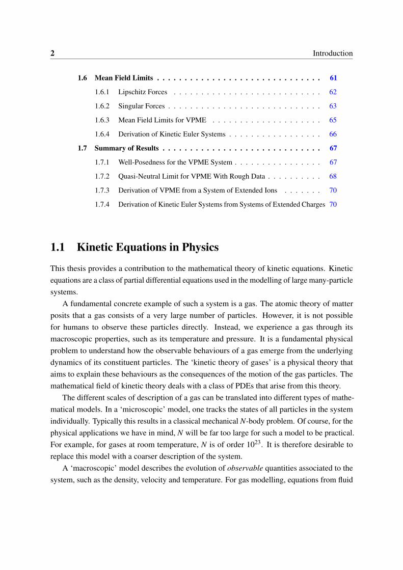
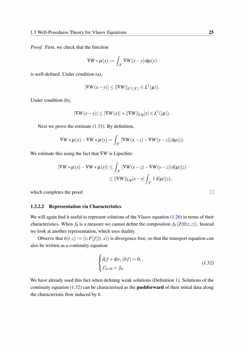
Large N Hydrodynamic Limit
Fluid MechanicsKinetic ModelParticle Model
Derivation of Fluid Equations
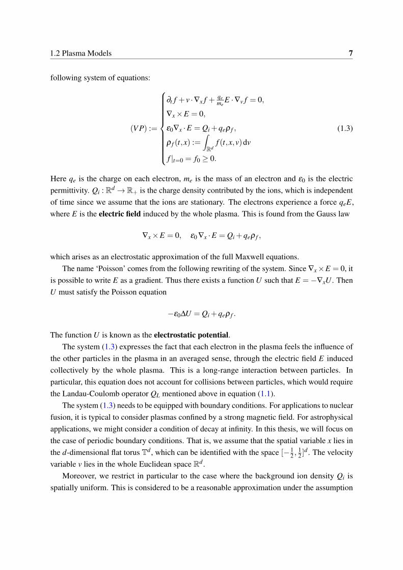
Fig. 1.1 Microscopic to macroscopic hierarchy for kinetic equations
It is a key problem in mathematical kinetic theory to justify the place of a kinetic equationin this hierarchy of models. On the one hand, we wish to derive kinetic equations from theunderlying models they describe; this validates the use of the equation from a mathematicalperspective. On the other hand, we wish to connect kinetic models to higher level macroscopicmodels, through hydrodynamic limits. This provides a possible strategy for deriving macro-scopic models, such as the equations of fluid dynamics, from particle models - by passing viaan intervening kinetic model.
The origins of modern kinetic theory are usually traced to the work of Maxwell [69] onthe modelling of gases. In this work, Maxwell derived a version of the Boltzmann equationfor dilute gases and identified its equilibrium distribution. Boltzmann [14] generalised thiswork and derived the ‘H-theorem’, which says that the (physical) entropy of solutions of theBoltzmann equation that are not in equilibrium must increase over time. The Boltzmannequation gives a mesoscopic description of a system of particles that interact with each otherthrough collisions and otherwise move freely. It takes the form
∂t f + v ·∇x f = Q( f ),
where Q is a nonlinear integral operator, acting in v only, that describes the change in f due tocollisions. Notice that the interaction between particles in this model is localised in x.
4 Introduction
Subsequently, Jeans [58] proposed a kinetic model to describe large systems of starsinteracting through gravity. This model is now referred to as the gravitational Vlasov-Poissonsystem. In contrast to the Boltzmann equation, this is a collisionless model. In this thesis,we will consider the electrostatic Vlasov-Poisson system, which is very closely related to theequation proposed by Jeans.
The principal focus of this thesis will be on kinetic equations that arise in the modellingof plasma. A plasma is an ionised gas, which means that it consists of charged particles. Theinteraction between these particles is thus electromagnetic in nature. An important differencebetween electromagnetic interactions and interaction through collisions is that electromagneticforces are long range. Charged particles influence each other even if the spatial separationbetween them is large. For this reason, the models typically used for ionised gases have adifferent structure from those typically used for electrically neutral gases.
Landau [60] proposed a kinetic model to describe the evolution of a plasma, now known asthe Landau-Coulomb equation. This model is based on adapting the Boltzmann equation tothe case of Coulomb interaction, and thus focuses on describing collisions within a plasma. Ittakes the form
∂t f + v ·∇x f = QL( f ), (1.1)
where QL( f ) denotes the nonlinear Landau collision operator.Vlasov [84, 85] proposed an alternative kinetic model for plasma. This equation takes the
form∂t f + v ·∇x f +(E + v×B) ·∇v f = 0, (1.2)
where E and B are, respectively, the electric and magnetic fields generated by the plasmaitself. The fields E and B are found using the Maxwell equations. This interaction is thereforenon-local in space, representing the fact that particles feel the influence of other particlesin the system even if their spatial separation is large. The system (1.2) is known as the(non-relativistic) Vlasov-Maxwell system.
In [84], Vlasov first considers a version of (1.2) that includes a term accounting for collisions.However, he then argues that on the physical scales relevant to plasma, the collision terms canbe neglected. This illustrates an important principle: the ‘correct’ model to use for a physicalsystem is not fixed solely based on the type of interactions in the system, but rather dependsalso on the physical regime in which the system is considered. For this reason, quantitativeresults are important in the study of hierarchies such as Figure 1.1. They allow us to identify,from a mathematical perspective, the timescales and regimes of physical parameters on whichthe models are valid.

1.1 Kinetic Equations in Physics 5
The central equation we consider in this thesis is a kinetic model for the ions in an unmag-netised plasma. It is known as the Vlasov-Poisson system with massless electrons, or VPME.This is a non-collisional model, similar in structure to (1.2). It is a variant of the better-knownVlasov-Poisson system, which models the electrons in an unmagnetised plasma. Our goal isto consider a hierarchy of models similar to the one shown in Figure 1.1, centred around theVPME system.
The macroscopic limit considered in this thesis is known as the quasi-neutral limit. This isnot a hydrodynamic limit, because the limiting equation is still a kinetic model. However, ourstudy is intended to be in a similar spirit to this framework: we will derive the macroscopicmodel from an underlying kinetic model, and use this to connect the macroscopic modelto a particle system. The macroscopic limit we consider is motivated by a widely usedapproximation in plasma physics, known as quasi-neutrality. In this approximation, a keycharacteristic parameter of the plasma, known as the Debye length, is set to zero. Under thisapproximation, equations of the form (1.2) are replaced by kinetic equations with a moresingular type of interaction. In this thesis we refer to these equations as ‘kinetic Euler’ systems.The mathematical study of the quasi-neutral limit is motivated by the need to identify thephysical regime in which this approximation is indeed valid.
Large N
‘Mean field’
Small Debye length
‘Quasi-neutral’
Ion Dynamics VPME Kinetic Euler
Fig. 1.2 Microscopic to macroscopic hierarchy for the VPME system
An important step in this investigation is to study the well-posedness of the VPME system.Before studying solutions of the VPME system, we wish to prove that such solutions exist andare unique for a given initial datum. Previously, global-in-time well-posedness results were notavailable for the VPME system in any dimension higher than one. In Chapter 2 of this thesis,we fill this gap by proving global well-posedness for the VPME system in dimension two andthree.
Moreover, we develop a key toolbox of estimates on the electric field for the VPME system,which allow many results for the Vlasov-Poisson system to be adapted to the VPME case. Wedemonstrate this in our study of the hierarchy shown in Figure 1.2, where these estimates arekey element. In Chapter 3, we prove a rigorous limit from the VPME system to a kinetic Eulermodel. In Chapter 4, we derive the VPME system from a microscopic system of extendedcharges. In Chapter 5, we combine these limits to identify a physical regime in which thekinetic Euler system can be derived from a system of extended charges.

6 Introduction
1.2 Plasma Models
1.2.1 The Vlasov-Poisson System
In this thesis, we will focus primarily on kinetic equations arising in the modelling of plasma.Plasma is a state of matter that forms when an electrically neutral gas is subjected to hightemperatures or a strong electromagnetic field. This causes some of the gas particles todissociate, splitting apart into charged particles. The resulting system is an ionised gas.
Plasma is abundant in the universe. The study of plasma is important in astrophysics - inspace, plasma is found for example in stars, the solar wind and the interstellar medium. Plasmais also studied as part of research into nuclear fusion reactors.
The degree of ionisation - that is, the fraction of gas particles that dissociate - varies inreal plasmas. In this thesis, we will concentrate on models that describe only the chargedspecies in the plasma, neglecting the neutral species that do not dissociate. The interactionswith the neutral species are very weak in comparison to the interactions of the charged species.There are two types of charged particle in a plasma: negatively charged electrons and positivelycharged ions.
The relevant physical situation to keep in mind is therefore a coupled system of ions andelectrons. Since these particles are charged, they will interact with each other principallythrough electromagnetic forces. In fact, it is usual to make an assumption which decouples thedynamics of the two species. This assumption is based on the fact that the mass of an electronis much smaller than the mass of an ion. Consequently, an electron typically moves much morequickly than an ion. This results in a separation between the timescales on which each speciesevolves.
Consider first the point of view of the electrons. The ions are, relatively speaking, muchmore massive and therefore slow moving. For this reason, it is common to assume that the ionsare stationary over the interval of time on which the plasma is observed. It remains to modelthe dynamics of the electrons.
The Vlasov-Poisson system is a well-known kinetic equation describing this situation.The electrons are described by a density function f = f (t,x,v), which is the unknown in the
1.2 Plasma Models 7
following system of equations:
(V P) :=
∂t f + v ·∇x f + qeme
E ·∇v f = 0,
∇x ×E = 0,
ε0∇x ·E = Qi +qeρ f ,
ρ f (t,x) :=∫Rd
f (t,x,v)dv
f |t=0 = f0 ≥ 0.
(1.3)
Here qe is the charge on each electron, me is the mass of an electron and ε0 is the electricpermittivity. Qi : Rd → R+ is the charge density contributed by the ions, which is independentof time since we assume that the ions are stationary. The electrons experience a force qeE,where E is the electric field induced by the whole plasma. This is found from the Gauss law
∇x ×E = 0, ε0 ∇x ·E = Qi +qeρ f ,
which arises as an electrostatic approximation of the full Maxwell equations.The name ‘Poisson’ comes from the following rewriting of the system. Since ∇x×E = 0, it
is possible to write E as a gradient. Thus there exists a function U such that E =−∇xU . ThenU must satisfy the Poisson equation
−ε0∆U = Qi +qeρ f .
The function U is known as the electrostatic potential.The system (1.3) expresses the fact that each electron in the plasma feels the influence of
the other particles in the plasma in an averaged sense, through the electric field E inducedcollectively by the whole plasma. This is a long-range interaction between particles. Inparticular, this equation does not account for collisions between particles, which would requirethe Landau-Coulomb operator QL mentioned above in equation (1.1).
The system (1.3) needs to be equipped with boundary conditions. For applications to nuclearfusion, it is typical to consider plasmas confined by a strong magnetic field. For astrophysicalapplications, we might consider a condition of decay at infinity. In this thesis, we will focus onthe case of periodic boundary conditions. That is, we assume that the spatial variable x lies inthe d-dimensional flat torus Td , which can be identified with the space [−1
2 ,12 ]
d . The velocityvariable v lies in the whole Euclidean space Rd .
Moreover, we restrict in particular to the case where the background ion density Qi isspatially uniform. This is considered to be a reasonable approximation under the assumption

8 Introduction
that the scale of fluctuations in the ion density is much larger than the scale of fluctuations inthe electron density. This results in the system
(V P) :=
∂t f + v ·∇x f + qeme
E ·∇v f = 0,
∇x ×E = 0,
ε0∇x ·E = qe(ρ f −∫Td×Rd
f dxdv),
f |t=0 = f0 ≥ 0.
(1.4)
The ion charge density is chosen to be
Qi ≡−qe
∫Td×Rd
f dxdv
so that the system is globally neutral. This is required by the conservation of charge, since theplasma forms from an electrically neutral gas. In mathematical treatments, it is common to see(1.4) written in the rescaled form
(V P) :=
∂t f + v ·∇x f +E ·∇v f = 0,
∇x ×E = 0,
−∇x ·E = ρ f −1,
f |t=0 = f0,∫Td×Rd
f0 dxdv = 1.
(1.5)
Another commonly considered form of the system is the case where the spatial variable xlies in the whole space Rd . In this case the boundary condition is that the electric field shoulddecay at infinity. The electric field can then be represented as the convolution of ρ f with theCoulomb kernel
K(x) =Cdx
|x|d.
The system then reads as follows:∂t f + v ·∇x f +E ·∇v f = 0,
E(x) =Cd
∫y∈Rd
x− y|x− y|d
ρ f (y)dy,
f |t=0 = f0 ≥ 0,∫Rd×Rd
f0 dxdv = 1.
(1.6)
1.2 Plasma Models 9
In this case, if we included a uniformly distributed background of ions this would result ina system with infinite mass. It is therefore usual to consider a system describing only thedynamics of electrons, resulting in a uniformly vanishing background.
By changing the sign in the equation for E in (1.6), we obtain a model for a system withgravitational interaction:
∂t f + v ·∇x f +E ·∇v f = 0,
E(x) =−Cd
∫y∈Rd
x− y|x− y|d
ρ f (y)dy,
f |t=0 = f0 ≥ 0,∫Rd×Rd
f0 dxdv = 1.
This model is used to describe, for example, the dynamics of large collections of stars. It wasdiscovered by Jeans [58]. We do not consider gravitational Vlasov-Poisson systems in thisthesis.
1.2.2 The Massless Electron Model
The classical version of the Vlasov-Poisson system, which was presented above, describesthe electrons in a dilute, unmagnetised plasma. We may instead wish to model the ions in theplasma. This leads to a variant of the Vlasov-Poisson system that will be the second mainequation considered in this thesis.
From the point of view of the ions, the electrons have a very small mass and so are very fastmoving. It is not possible to assume that they are stationary. Instead, we observe that, since theelectrons move quickly relative to the ions, the frequency of electron-electron collisions will behigh in comparison to other kinds of collisions, and electron-electron collisions are relevantand frequent on the typical timescale of evolution of the ions. It is therefore common in physicsliterature to assume that the electrons are close to thermal equilibrium.
The limit of massless electrons is the limit in which the ratio between the masses of theelectrons and ions, me/mi, tends to zero. Here me is the mass of an electron and mi is themass of an ion. This limit is physically relevant due to the large disparity in mass between theions and electrons. In this limit, it is assumed that the electrons instantaneously assume theequilibrium distribution.
The equilibrium distribution can be identified by studying the equation for the evolution ofelectrons. Let the ion density ρ[ fi] be fixed, and assume that all ions carry the same charge qi.We have discussed that the evolution of the electron density can be modelled by the Vlasov-Poisson system (1.3). As discussed above, in the long time regime we consider we expect theeffect of electron-electron collisions to be significant. We therefore augment the system (1.3)

10 Introduction
with a collision operator. Bellan [11, Chapter 13, Equation (13.46)] suggests the followingrescaling of the Landau-Coulomb operator for modelling collisions in a plasma:
Qelec( f ) =Ce
m2e
QL( f ),
where Ce is a constant depending on physical quantities such as the electron charge qe andnumber density ne, but not on the electron mass me. The Landau-Coulomb operator QL isdefined as follows: for a given function g = g(v) : Rd → R,
QL(g) := ∇v ·∫Rd
a(v− v∗) : [g(v∗)∇vg(v)−g(v)∇vg(v∗)]dv∗.
The tensor a is defined by
a(z) =|z|2 − z⊗ z
|z|3.
We thus consider the following model for the electron density fe, here posed on the torusx ∈ Td:
∂t fe + v ·∇x fe +qe
meE ·∇v fe =
Ce
m2e
QL( fe),
∇x ×E = 0, ε0∇x ·E = qiρ[ fi]+qeρ[ fe].(1.7)
Consider the rescaling in velocity
Fe(t,x,v) = m− d
2e fe
(t,x,
v√
me
).
Notice that ρ[Fe] = ρ[ fe]. Then Fe satisfies √me∂tFe + v ·∇xFe +qeE ·∇vFe =CeQL(Fe),
∇×E = 0, ε0∇ ·E = qiρ[ fi]+qeρ[Fe].(1.8)
We assume that Fe converges to a stationary distribution fe = fe(x,v) as me tends to zero, andfocus on formally identifying fe.
We expect that fe should satisfy the equation
v ·∇x fe +qeE ·∇v fe =CeQL( fe).
By considering the following entropy functional
H[ f ] =∫
f log f dxdv,
1.2 Plasma Models 11
which is non-increasing for solutions of (1.8), it is possible to show that fe should be a localMaxwellian of the form
fe(x,v) = ρe(x)(πβe(x))d/2 exp
[−βe(x)|v−ue(x)|2
], (1.9)
since these are precisely the distributions for which the time derivative of the entropy vanishes.The electron density ρe, mean velocity ue and inverse temperature βe can then be studied usingan argument similar to the one given in the proof of [7, Theorem 1.1].
Substituting the form (1.9) into equation (1.7), we obtain the following identity for all xsuch that ρe(x) = 0 and all v ∈ Rd:
−∇xβe · (v−ue)|v−ue|2 −ue ·∇xβe|v−ue|2 +βe(v−ue)⊤
∇xue(v−ue)
+(v−ue) ·[∇x log(ρeβ
d/2e )−qeβeE +ue ·∇xue
]+ue ·∇x log(ρeβ
d/2e ) = 0.
For each fixed x, the left hand side is a polynomial in v−ue(x), whose coefficients must allbe equal to zero. For example, by looking at the cubic term we see that ∇xβe = 0 and thus βe
must be a constant independent of x.The quadratic term then gives
v⊤∇xuev = 0 for all v ∈ Rd,
which implies that ∇xue is skew-symmetric. On a spatial domain for which a Korn inequalityholds, it is possible to restrict which ue can occur. For example, in the case of the torus x ∈ Td
considered, the fact that the symmetric part of ∇xue vanishes implies that ue is constant [25,Proposition 13].
Finally, from the linear term we obtain that
∇x log(ρeβd/2e )−qeβeE = 0.
Since ∇x ×E = 0, E is a gradient - that is, it can be written as E =−∇U for some function U .Then
∇x log(ρeβd/2e ) =−qeβe∇xU.
From this we deduce that ρe should be of the form
ρe(x) = Aexp(−qeβeU) ,
for some constant A > 0. This is known as a Maxwell-Boltzmann law.
12 Introduction
Since ∇x ×E = 0, we can write E =−∇xU , where U is the electrostatic potential withinthe plasma. Then
∇xρe =− qe
kBTeρe∇xU.
From this we deduce that ρe should be of the form
ρe(x) = Aexp(−qeU(x)
kBTe
),
which is known as a Maxwell–Boltzmann law.See Bardos et al. [7] for rigorous results on identifying the Maxwell-Boltzmann law as
the limiting distribution of the electrons in the massless limit, for Vlasov-Poisson models withcollision operators of Boltzmann or BGK type.
From equation (1.7), we see that the electrostatic potential U should satisfy the followingsemilinear elliptic PDE:
−ε0∆U = qiρ[ fi]+Aqe exp(− qeU
kBTe
). (1.10)
The normalising constant A is chosen so that the system is globally neutral, that is, the totalcharge is zero: ∫
Tdqiρ[ fi]+Aqe exp
(− qeU
kBTe
)dx = 0.
The equation (1.10) replaces the standard Poisson equation for the electrostatic potentialin the Vlasov-Poisson system (1.3). After a suitable normalisation of physical constants, thisleads to the following system for the ions:
(V PME) :=
∂t f + v ·∇x f +E ·∇v f = 0,
E =−∇xU,
∆U = eU −ρ f ,
f |t=0 = f0,∫Td×Rd
f0 dxdv = 1.
(1.11)
This is known as the Vlasov-Poisson system with massless electrons, or VPME.Note that solutions of the system (1.11) always satisfy global neutrality, since on the torus
the Poisson equation∆U = h
can only be solved if h has total integral zero.
1.2 Plasma Models 13
The VPME system has been used in the physics literature in, for instance, numerical studiesof the formation of ion-acoustic shocks [68, 77] and the development of phase-space vorticesbehind such shocks [15], as well as in studies of the expansion of plasma into vacuum [70]. Aphysically oriented introduction to the model (1.11) may be found in [40].
This system is one of the central equations considered in this thesis. We will investigateseveral mathematical questions related to this system. Chapter 2 focuses on the problem ofshowing global well-posedness for this equation in dimension two and three. We then lookat two limits relating the VPME system to other models for the ions in a plasma. One is thequasi-neutral limit, which connects the VPME system (1.11) to a macroscopic model for theplasma. The other is the mean field limit, in which the aim is to derive the VPME system froman underlying system of interacting particles.
1.2.3 Quasi-Neutrality
Quasi-neutrality is a concept from plasma physics, referring to a situation in which a certaincharacteristic scale of the plasma is small. This property occurs frequently in real plasmas. Wewill use this idea to motivate a mathematical problem known as the quasi-neutral limit. This isa limit in which one can derive other plasma models from the Vlasov-Poisson systems, under acertain rescaling.
1.2.3.1 The Debye Length
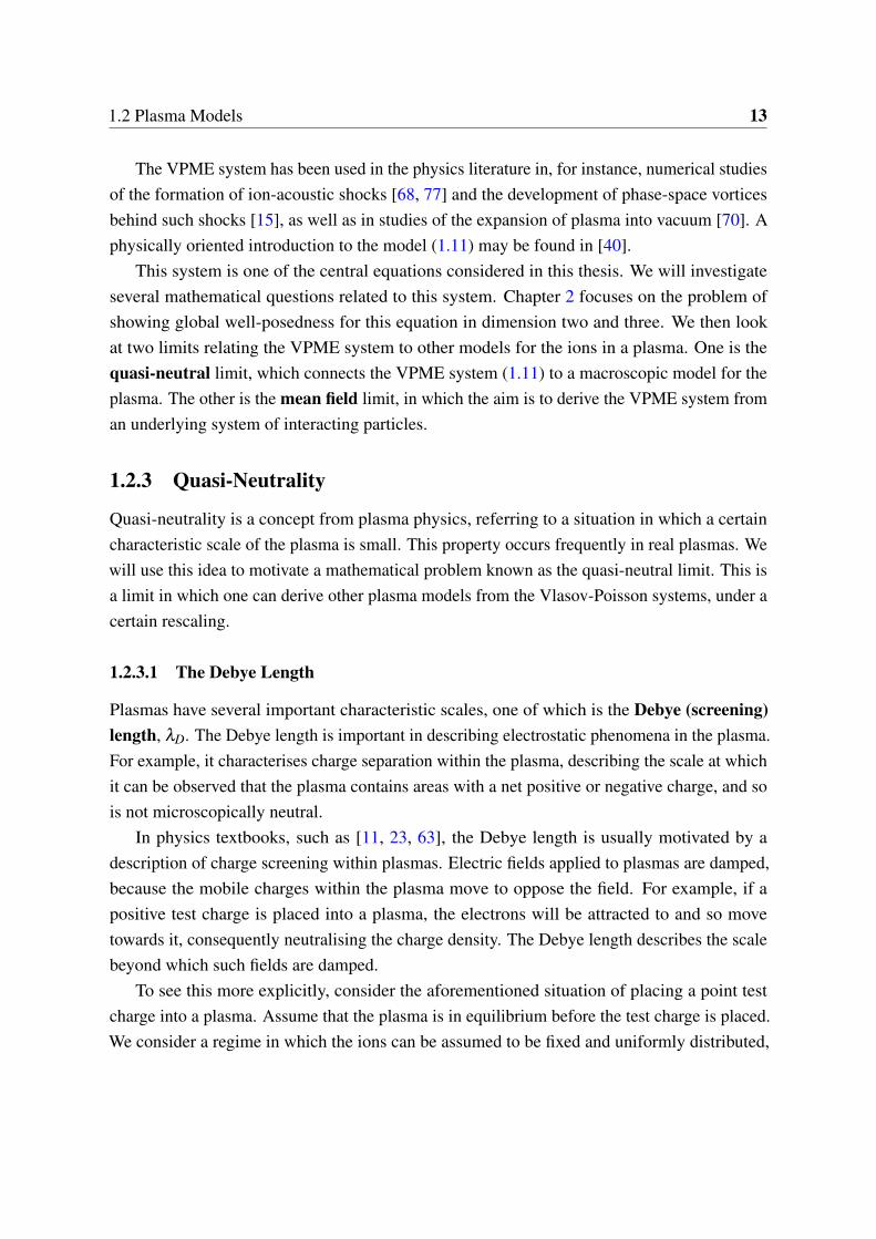
Plasmas have several important characteristic scales, one of which is the Debye (screening)length, λD. The Debye length is important in describing electrostatic phenomena in the plasma.For example, it characterises charge separation within the plasma, describing the scale at whichit can be observed that the plasma contains areas with a net positive or negative charge, and sois not microscopically neutral.
In physics textbooks, such as [11, 23, 63], the Debye length is usually motivated by adescription of charge screening within plasmas. Electric fields applied to plasmas are damped,because the mobile charges within the plasma move to oppose the field. For example, if apositive test charge is placed into a plasma, the electrons will be attracted to and so movetowards it, consequently neutralising the charge density. The Debye length describes the scalebeyond which such fields are damped.
To see this more explicitly, consider the aforementioned situation of placing a point testcharge into a plasma. Assume that the plasma is in equilibrium before the test charge is placed.We consider a regime in which the ions can be assumed to be fixed and uniformly distributed,
14 Introduction
and we only take the motion of the electrons into account. We assume that their motion is fastenough that the electrons are always thermalised.
We consider placing a point test charge of charge β at the origin. When the charge is added,it induces a potential Φ. In response, the electrons take on a Maxwell-Boltzmann distribution.Their spatial density is therefore
ρe = ne exp(
qeΦ
kBTe
),
where qe is the charge on an electron, kB is the Boltzmann constant and Te is the electrontemperature and ne is the spatial density of electrons prior to the introduction of the test charge.The normalisation ne is chosen because the potential Φ should decay in the far field. Thepotential Φ should solve the following equation:
ε0∆Φ = neqe
(exp(
qeΦ
kBTe
)−1)−β δ0,
where δ0 denotes the Dirac distribution.By rescaling this equation, we can identify key parameters. Let Φ := qeΦ
kBTe. Then
ε0kBTe
neq2e
∆Φ = eΦ −1− β
neqeδ0. (1.12)
This motivatives defining a scale λD by
λD :=(
ε0kBTe
neq2e
)1/2
. (1.13)
This scale is the Debye length associated to the electrons. Equation (1.12) then becomes
λ2D ∆Φ = eΦ −1− β
neqeδ0.
From the structure of this equation we can see that λD is important in determining the shape ofthe potential. More explicitly, Φ is then of the form Φ(x) = Ψ
(x
λD
), where Ψ is a solution of
the following equation:
∆Ψ = eΨ −1− β
neqeλ dD
δ0. (1.14)
1.2 Plasma Models 15
To see the screening effect, in standard physics presentations it is common to lineariseequation (1.14) to obtain
∆Ψ = Ψ− β
neqeλ dD
δ0.
Using the symmetry of the problem, it is possible to derive an explicit formula for Ψ (see forexample [11]). In dimension d = 3 this is
Ψ(x) =β
4π
1nqeλ 3
D
e−|x|
|x|.
Then Φ takes the form
Φ(x) =β
4π
kBTe
nq2e
λ−2D
e−|x|λD
|x|=
β
4πε0
e−|x|λD
|x|,
which is known as the Yukawa potential. The decay of Φ demonstrates the shielding effectdescribed earlier: the typical length of spatial decay of Φ is of order λD.
If we consider a timescale on which the ions are significantly mobile, it is possible toperform a similar analysis in which the motion of ions also plays a role in this screening effect.The ions will then have an associated Debye length, which may differ from the electron Debyelength. It is defined by the formula (1.13), replacing the the electron density, temperature andcharge with the corresponding values for the ions.
Since the Debye length is related to observable quantities such as the density and tempera-ture, it can be found for a real plasma. Typically, λD is much smaller than the typical lengthscale of observation L. The parameter
ε :=λD
L
is therefore expected to be small. In this case the plasma is called quasi-neutral - since thescale of charge separation is small, the plasma appears to be neutral at the scale of observation.
Quasi-neutrality is a very common property of real plasmas, to the point that some referencesinclude quasi-neutrality as part of the definition of a plasma. For example, Chen [23, Section1.2] includes quasi-neutrality as one of the key properties distinguishing plasmas from ionisedgases more generally. In plasma physics literature, the approximation that ε ≈ 0 is widely used.For this reason, it is important to understand what happens to the Vlasov-Poisson system in thelimit as ε tends to zero. This is known as the quasi-neutral limit.

16 Introduction
1.2.3.2 The Debye Length in the Vlasov-Poisson System
When written in appropriate dimensionless variables, the classical Vlasov-Poisson system (1.5)takes the form
(V P)ε :=
∂t f + v ·∇x f +E ·∇v f = 0,
E =−∇xU,
−ε2∆U = ρ f −1,
f |t=0 = f0,∫Td×Rd
f0(x,v)dxdv = 1.
(1.15)
In equation (1.15) we can see that the relative Debye length ε indeed appears as a parameterdescribing the scale of the electric field E. In physics literature, it is common to work under theassumption that ε ≈ 0. This leads to another model.
1.2.3.3 Kinetic Euler Systems
Formally setting ε = 0 in the system (1.15) results in the following system:
(KInE) :=
∂t f + v ·∇x f −∇xU ·∇v f = 0,
ρ f = 1,
f |t=0 = f0,∫Td×Rd
f0(x,v)dxdv = 1.
(1.16)
This is an example of a kinetic Euler system. In system (1.16) the force −∇xU is now definedimplicitly through the constraint ρ f = 1, rather than explicitly through the Poisson equation, asin (1.15). It is akin to a pressure term in a fluid equation.
The system (1.16) was discussed by Brenier [19] as a kinetic formulation of the incom-pressible Euler equations. The correspondence can be seen clearly by considering monokineticsolutions of (1.16), which are solutions of the form
f (t,x,v) = ρ(t,x)δ0(v−u(t,x)) (1.17)
for some density ρ and velocity field u. If f of the form (1.17) is a solution of (1.16), then u isin turn a solution of the incompressible Euler equations:
(InE) :=
∂tu+u ·∇xu−∇xU = 0,
∇x ·u = 0.(1.18)
1.2 Plasma Models 17
This observation illustrates the reason for calling (1.16) an ‘Euler’ equation. We will refer to(1.16) as the kinetic incompressible Euler system, to distinguish it from other kinetic Eulersystems we will introduce below.
It is also possible to consider the quasi-neutral limit for the VPME system. In this case, thescaled system is
(V PME)ε :=
∂t f + v ·∇x f +E ·∇v f = 0,
E =−∇xU,
ε2∆U = eU −ρ f ,
f |t=0 = f0,∫Td×Rd
f0(x,v)dxdv = 1.
(1.19)
The formal limit is another kinetic Euler system:
(KIsE) :=
∂t f + v ·∇x f −∇xU ·∇v f = 0,
U = logρ f ,
f |t=0 = f0,∫Td×Rd
f0(x,v)dxdv = 1.
(1.20)
This system was introduced and studied in a physics context in [38–40]. For monokineticsolutions of (1.20), the pair (ρ,u) satisfies the following isothermal Euler system:
(IsE) :=
∂tρ +∇x · (ρu) = 0,
∂t (ρu)+∇x : (ρu⊗u)−∇xρ = 0.
We therefore refer to (1.20) as the kinetic isothermal Euler system.It is worth observing that, although we have introduced both KInE and KIsE under the
umbrella of ‘kinetic Euler systems’, these systems are structurally different. In the KIsE system(1.20), the force −∇xU depends on ρ f in an explicit, albeit singular, way. In the KInE system,the force is defined implicitly through the incompressibility constraint. This distinction issimilar to the difference between compressible and incompressible Euler equations, which isnot surprising considering the connection between these systems through the monokinetic case.
To understand the KIsE system, it is often instructive to consider a related system, namedVlasov–Dirac–Benney by Bardos [4]. This system can also be thought of as a kinetic Euler
18 Introduction
equation. The VDB system reads as follows:
(V DB) :=
∂t f + v ·∇x f −∇xU ·∇v f = 0,
U = ρ f −1
f |t=0 = f0,∫Td×Rd
f0(x,v)dxdv = 1.
(1.21)
It can be obtained by linearising the coupling U = logρ f between U and ρ f . As well as beinginteresting in its own right, the VDB system provides useful intuition for the KIsE system,since they have similar structures but the coupling between ∇xU and ρ f is linear for VDB.
1.2.3.4 The Quasi-Neutral Limit
Formal identification of the limiting system does not guarantee that equations (1.16) and(1.20) are good approximations for (1.15) and (1.19) when ε is small but non-zero. To showthis, it is necessary to study the quasi-neutral limit from each Vlasov-Poisson system to thecorresponding kinetic Euler system. It is not guaranteed that this approximation will always bevalid. Note, for example, that Medvedev [70] describes a situation in which the quasi-neutralapproximation U = logρ is not valid everywhere. This provides a physical motivation fora study of the transition between (1.19) and (1.20). In particular we would like to identifyconditions on the data and quantitative ranges of the physical parameters for which the limitholds. Results of this type identify regimes in which the limiting systems (1.16) and (1.20) canbe validated mathematically.
The rigorous mathematical justification of the quasi-neutral limit turns out to be a challeng-ing problem, requiring quite stringent restrictions on the initial data. The reasons for this areat least in part of physical origin. This will be discussed further in Section 1.5. In Chapter 3,we consider the quasi-neutral limit from VPME to the kinetic isothermal Euler system. Weare able to prove a rigorous quasi-neutral limit for a class of rough data, in dimension two andthree.
1.2.4 Derivation from a Particle System
It is a fundamental problem in the theory of kinetic equations to derive the PDE models, in arigorous way, from the underlying physical system they are meant to describe. For instance,consider the classical Vlasov-Poisson system (1.5), which we motivated as a model for theelectrons in a plasma. A lower level description of this system would be to consider a systemof N electrons, each modelled as a point particle with mass me and charge qe. The dynamics ofthe electrons can be described using the laws of classical mechanics. In this case, the state of

1.2 Plasma Models 19
the ith electron can be characterised by its position Xi and velocity Vi. For ease of presentation,here we consider this system evolving in the whole space without a background of ions. Theevolution of (Xi,Vi)
Ni=1 should then be described by the following system of ODEs: Xi =Vi
Vi =1
meE(Xi;X j j =i
),
(1.22)
where E(Xi;X j j =i
)is the electrostatic force exerted on electron i by the other electrons in the
plasma. The force exerted on electron i by electron j is given by the Coulomb force betweenpoint charges; in three dimensions this is
q2e
4πε0
Xi −X j
|Xi −X j|3,
where ε0 denotes the vacuum permittivity. We use the notation K for the function
K(x) =x
4π|x|3.
Then the particle system (1.22) becomesXi =Vi
Vi =− q2e
me∑j =i
K(Xi −X j
).
After an appropriate non-dimensionalisation, we reach the systemXi =Vi
Vi =−α ∑j =i
K(Xi −X j
),
(1.23)
where the parameter α is a function of the physical constants of the plasma.We would like to show that the PDE model (1.6) gives a good description of the limiting
behaviour of the particle system (1.23) as N tends to infinity. To do this it is necessary to rescalethe system, which means choosing α to vary with N. The choice of scaling α = α(N) affectsthe kind of limit we can obtain.
In order to derive the Vlasov-Poisson system (1.6), the appropriate choice is the mean fieldscaling α(N) = 1/N. With this choice, formally speaking, the Vlasov-Poisson system appearsto describe the limiting behaviour of (1.23). This connection between the particle system (1.23)and the PDE (1.6) is called the mean field limit. However, whether this limit truly holds is
20 Introduction
an open problem, and it may be false in some regimes. In Section 1.6, we will discuss thetechnical obstacles to this limit in greater detail, and give an overview of recent approaches tothis problem.
Similar issues affect the derivation of the VPME model for ions. In this case, for themicroscopic model we consider a system of ions, modelled as point particles, in a backgroundof thermalised electrons. The assumption of thermalisation is justified by the difference betweenthe typical timescales of the ions and electrons. This is modelled by an ODE system of theform
Xi =Vi
Vi =− 1N ∑
j =iK(Xi −X j
)+K ∗ eU , (1.24)
where U is the electrostatic potential induced by the ions and the background of electrons. Thatis, U satisfies
∆U = eU − 1N
N
∑i=1
δXi. (1.25)
As in the classical case, the rigorous derivation of the VPME system from the particlesystem (1.24) remains an open problem. However, in Chapter 4 we will prove a rigorousderivation of the VPME system from a regularised version of (1.24).
If we consider a different choice of scaling α(N), then it may be possible to obtain differentPDE models in the limit. Recall for example the hierarchy of plasma models that we laid out inFigure 1.2. By using a different scaling of α than the mean field scaling, it is possible to passfrom the particle model to the kinetic Euler system KIsE (1.20), rather than the VPME system.We investigate this direction in Chapter 5, where we derive the kinetic Euler systems fromregularised particle systems, under an alternative scaling. For example, for the KInE system(1.16) we use a scaling of the form
α(N) =C(logN)κ
N,
for some exponent κ stated in Theorem 1.26 in Section 1.7. For the KIsE system (1.20) we usea scaling of the form
α(N) =Clog loglogN
N.

1.3 Well-Posedness Theory for Vlasov Equations 21
1.3 Well-Posedness Theory for Vlasov Equations
The Vlasov-Poisson system is an example of a nonlinear scalar transport equation. In particularit belongs to a class of PDEs known as Vlasov equations. The aim of this section is tointroduce this class of equations and to review some of the fundamental concepts involved intheir well-posedness theory. For further details, we refer to the notes of Golse [31].
1.3.1 Vlasov Equations
Vlasov equations are used to model large systems of interacting particles. Below is a generalexample:
∂t f + v ·∇x f +F [ f ] ·∇v f = 0,
F [ f ](t,x) =−∇xW ∗ρ f ,
ρ f (t,x) =∫Rd
f (t,x,v)dv,
f (0,x,v) = f0(x,v)≥ 0.
(1.26)
The unknown f = f (t,x,v) represents the density of particles at time t which have positionx and velocity v. In this thesis, we will only discuss the problem posed on domains withoutboundary, letting (x,v) ∈ X ×Rd , where either X = Rd (the whole space case) or X = Td
(the periodic case).Equation (1.26) describes a system in which particles influence each other through pairwise
interactions. The interaction between two particles is described by a pair potential W dependingonly on the separation between the particles in position space. The force exerted on a particleat position x by another particle at position y is therefore −∇xW (x− y). For example, theVlasov-Poisson case can be obtained by choosing W to be the Green’s function of the Laplacianon X . In the limit as the number of particles tends to infinity, this results in an effective forceF [ f ] as defined in (1.26). In Section 1.6 we will discuss the connection between the PDE(1.26) and the underlying particle system in more detail. In this section, we will focus on thewell-posedness theory of the PDE (1.26).
1.3.1.1 Transport Equations
The basic underlying structure of (1.26) is that of a scalar transport equation. Letting z = (x,v),equation (1.26) is of the form ∂t f +b ·∇z f = 0,
f (0,z) = f0(z).(1.27)
22 Introduction
whereb(t,z) := (v,F [ f ](t,x)) .
The fact that the force F , and therefore b, depends on f is what creates the nonlinearity in(1.26).
In this section, we will discuss some aspects of the theory of the linear equation (1.27),which will be useful for understanding the nonlinear Vlasov equation. The properties of thetransport equation (1.27) clearly depend on the choice of the vector field b. For proving well-posedness, what is important to understand is the regularity of b. One way to understand this isthrough the classical method of characteristics.
The transport equation (1.27) is associated with a family of characteristics. A path (Z(t))t∈Rin phase space is a characteristic trajectory for equation (1.27) if it satisfies the ODE
dZdt
= b(t,Z) . (1.28)
The characteristics are a useful tool for understanding the behaviour of equations like (1.27)- see for example [24] for a more detailed exposition of this theory. We will make use ofcharacteristics in many places in this thesis. We will use the notation Z(t;s,z) to denote asolution of (1.28) which has phase space position z at time s; that is, Z(s;s,z) = z = (x,v).
If b is sufficiently regular, then the system (1.28) has a unique global-in-time solution forany choice of data (s,x,v). For example, this will be the case if b is continuous in all variablesand Lipschitz with respect to z, with less than linear growth:
|b(t,z1)−b(t,z2)| ≤ L|z1 − z2|, |b(t,z)| ≤C(1+ |z|). (1.29)
In this case the characteristic trajectories can be used to construct solutions of the transportequation (1.27). Suppose for example that f0 is a C1 function with compact support. Then(1.27) has a unique solution ft which can be represented by the formula
f (t,z) = f0 (Z(0; t,z)) .
This shows that the equation (1.27) indeed models the transport of mass along this family ofcurves.
The representation of the solution f in terms of characteristics is useful for understandingits properties. For example, it immediately implies that the equation preserves sign: if f0 ≥ 0,then also ft ≥ 0 for all t. Similarly, the L∞(X ×Rd) norm of the solution cannot grow over

1.3 Well-Posedness Theory for Vlasov Equations 23
time: if f0 ∈ L∞(X ×Rd), then also ft ∈ L∞(X ×Rd) with
∥ f (t, ·)∥L∞(X ×Rd) ≤ ∥ f0∥L∞(X ×Rd).
If b is less regular than specified in condition (1.29), then for both the ODE (1.28) and thePDE (1.27) solutions may not exist globally and may not be unique without further assumptions.The well-posedness theory of the ODE (1.28) under weaker regularity conditions than (1.29)was considered by DiPerna and Lions [26], by making use of the connection between the ODEand the corresponding transport equation (1.27). This strategy was then extended in many otherworks; for more details on this subject see for example Ambrosio [1].
In the context of Vlasov equations, the lesson is that the well-posedness theory of thetransport equation (1.27) depends crucially on the regularity of the vector field b. Consequently,for the nonlinear Vlasov equation, it will be important to understand the regularity of the forceF [ f ] and how that regularity depends on properties of f . This depends on the regularity of theinteraction potential W .
1.3.2 Regular Potentials
When W is sufficiently regular, the Vlasov equation (1.26) has a well developed well-posednesstheory. In particular, when ∇xW is a Lipschitz function, it is possible to construct unique globalsolutions to the Vlasov equation (1.26), assuming very little regularity on the initial datumf0. In fact it will be enough to suppose only that f0 is a probability measure with moments ofsufficiently high order.
The case where ∇xW is Lipschitz is thought of as the ‘regular’ case for Vlasov equations ofthe form (1.26). We will discuss this case here in some detail, as this will allow us to introduceseveral useful ideas in Vlasov equation theory that we will return to in the Vlasov-Poisson case.In particular, the aim is to understand how the assumption that ∇xW is Lipschitz is used in thewell-posedness results.
The immediate consequence of the Lipschitz assumption is that ∇xW ∗ρ is then a Lipschitzfunction, for any finite measure ρ , without further regularity assumptions. This means thateven measure solutions of (1.26) will have an associated classical characteristic flow. We willsee subsequently that this assumption on W also allows the construction of unique solutions forthe nonlinear problem (1.26).
Notation: Spaces of Measures. We are going to look for measure solutions of equation(1.26). We begin by specifying some notation for the class of solutions we are interested in.
24 Introduction
At each fixed time t, the solution should be measure on the phase space X ×Rd , wherethe position space X is either Rd or the torus Td . We denote the space of finite signed Borelmeasures on X ×Rd by M , and the space of finite (non-negative) measures by M+. We equipthese spaces with the topology of weak convergence of measures, in which a sequence (µn)n
converges to µ as n tends to infinity if and only if
limn→∞
∫X ×Rd
φ dµn =∫X ×Rd
φ dµ, ∀φ ∈Cb(X ×Rd).
Furthermore, M1 denotes the subspace of M consisting of all finite signed measures with afinite first moment: ∫
X ×Rd(|x|+ |v|)d|µ|(x,v)<+∞.
Similarly M+,1 = M1 ∩M+.The space C ([0,∞);M ) consists of paths t 7→ µ(t) ∈ M taking values in the space of
signed measures, where the continuity of the path is defined in terms of the topology of weakconvergence of measures. The spaces C ([0,∞);M+), C ([0,∞);M1) and C ([0,∞);M+,1)
are defined similarly. In the next section we will look for solutions of the Vlasov equation(1.26) in the space C ([0,∞);M+,1). We refer to such solutions informally as ‘measure-valuedsolutions’.
1.3.2.1 Weak Formulation
To make sense of measure solutions for equation (1.26), it is necessary to understand theequation in a weak sense.
Definition 1 (Weak Solutions). f ∈C ([0,∞);M+) is a weak solution of the Vlasov equation(1.26) if, for all test functions φ ∈C1
c([0,∞)×X ×Rd),∫
∞
0
∫X ×Rd
[∂tφ +v·∇xφ −
(∇xW ∗x ρ f
)·∇vφ
]f (t,dx,dv)dt+
∫X ×Rd
φ(0,x,v) f0(dx,dv)= 0.
(1.30)
In order for (1.30) to make sense, ∇xW ∗x ρ f must be regular enough that(∇xW ∗x ρ f
)·∇vφ
is integrable with respect to f . This is ensured by the following lemma, which shows that∇xW ∗x ρ f will be Lipschitz provided that ∇xW is Lipschitz.
Lemma 1.1. Let µ ∈ M (X ), and let ∇W be a Lipschitz function. Assume that either (a)∇W ∈ L∞(X ) or that (b) µ ∈ M1(X ). Then ∇W ∗µ is a Lipschitz function. Moreover, wehave the quantitative estimate
|∇W ∗µ(x)−∇W ∗µ(y)| ≤ ∥∇W∥Lip |µ|(X ) |x− y|. (1.31)
1.3 Well-Posedness Theory for Vlasov Equations 25
Proof. First, we check that the function
∇W ∗µ(x) :=∫X
∇W (x− y)dµ(y)
is well-defined. Under condition (a),
|∇W (x− y)| ≤ ∥∇W∥L∞(X ) ∈ L1(µ|).
Under condition (b),
|∇W (x− y)| ≤ |∇W (x)|+∥∇W∥Lip|y| ∈ L1(|µ|).
Next we prove the estimate (1.31). By definition,
∇W ∗µ(x)−∇W ∗µ(y) =∫X
[∇W (x− z)−∇W (y− z)]dµ(z).
We estimate this using the fact that ∇W is Lipschitz:
|∇W ∗µ(x)−∇W ∗µ(y)| ≤∫X
|∇W (x− z)−∇W (y− z)|d|µ|(z)
≤ ∥∇W∥Lip|x− y|∫X
1 d|µ|(z),
which completes the proof.
1.3.2.2 Representation via Characteristics
We will again find it useful to represent solutions of the Vlasov equation (1.26) in terms of theircharacteristics. When f0 is a measure we cannot define the composition f0 (Z(0; t,z)). Insteadwe look at another representation, which uses duality.
Observe that b(t,z) := (v,F [ f ](t,x)) is divergence free, so that the transport equation canalso be written as a continuity equation:∂t f +divz (b f ) = 0,
f |t=0 = f0.(1.32)
We have already used this fact when defining weak solutions (Definition 1). Solutions of thecontinuity equation (1.32) can be characterised as the pushforward of their initial data alongthe characteristic flow induced by b.

26 Introduction
Definition 2 (Pushforward). For i = 1,2, let (Ωi,Fi) be a measurable space. Let µ be ameasure on (Ω1,F1). Let T : Ω1 → Ω2 be a measurable map. The pushforward of µ alongT , denoted by T#µ , is the measure on (Ω2,F2) defined by the relation
T#µ(A) = µ(T −1(A)
), ∀A ∈ F2.
In particular, for all measurable functions g on Ω2 for which the composition gT is integrablewith respect to µ , the following relation holds:∫
Ω2
g dT#µ =∫
Ω1
gT dµ.
To represent solutions of the linear continuity equation (1.32), we will take T to bethe flow map induced by the characteristic system (1.28). The flow is a family of maps(Φs,t : X ×Rd → X ×Rd)s,t , defined by the property
Φs,t(z) = Z(t;s,z).
Then, if b satisfies (1.29), the continuity equation (1.32) has a unique solution f for any initialdatum f0 ∈ M+. Moreover, f has the representation ft = Φ
0,t# f0. That is, for all φ ∈Cc,∫
X ×Rdφ(z) f (t,dz) =
∫X ×Rd
φ(Φ
0,t(z))
f0(dz) =∫X ×Rd
φ (Z(t;0,z)) f0(dz). (1.33)
For proofs and further details, see [1, Proposition 4].
Conservation of Mass From the representation (1.33) it is clear that the equation conservesmass: for a continuous path f ∈C([0,∞);M+), ft has finite mass for all times t, and therefore(1.33) can be extended to the function φ ≡ 1. This implies that ft has the same total massas f0. The assumptions f0 ≥ 0 and
∫X ×Rd f0 dz = 1 thus ensure that, for each fixed t, ft is a
probability measure on X ×Rd .We let P denote the space of probability measures on X ×Rd , and P1 the space of
probability measures with a finite first moment. The discussion above shows that it is enoughto consider measure-valued solutions in the space C ([0,∞);P).
1.3.2.3 Existence of Solutions
We now turn to the existence of solutions for the nonlinear Vlasov equation (1.26). We refer tothe works [18, 27, 72, 31] for the following result.
1.3 Well-Posedness Theory for Vlasov Equations 27
Theorem 1.2. Assume that ∇W : X → Rd is a Lipschitz function. Let f0 ∈ P1. Then thereexists a solution f ∈C ([0,∞);P) of the Vlasov equation (1.26), in the sense of Definition 1.
The proof of this result presented here follows the presentation of [31, Theorem 1.3.1].The proof can be formulated as a fixed point problem: first, we decouple the nonlinearity andconsider the equation ∂tg+ v ·∇xg+F [ f ] ·∇vg = 0,
g|t=0 = f0.(1.34)
In equation (1.34), g is the unknown and f should be thought of as a fixed ‘input’. We havediscussed above that, for any f0 ∈ P , the solution g of equation (1.34) has the representationg = Φ0,·[ f ]# f0. A solution of the nonlinear Vlasov equation (1.26) can therefore be constructedby proving the existence of a fixed point of the map f 7→ Φ0,·[ f ]# f0.
In fact, we will look at the corresponding map on the flow Φ0,·[ f ]. We can think of Φ0,·[ f ]as an element of the space C
(R×X ×Rd). This can be made into a Banach space with an
appropriate choice of norm. For flows we want to consider the map T defined by
T [φ ] = Φ0,·[φ# f0].
If φ = T [φ ], then φ# f0 is a solution of the Vlasov equation (1.26) with initlal datum f0.To find such a fixed point, we can use a standard iteration argument. Set φ0 to be the
identity map on X ×Rd for all t, and consider the sequence (φn)n where φn+1 = T [φn]. Toprove that this iteration converges to a limit, it is enough to show that T is a contraction onC([0,T ];X ×Rd) for some T . We can then conclude that a fixed point exists by the standard
arguments for a Picard iteration.We equip C
([0,T ];X ×Rd) with the norm
∥φ∥YT := supt∈[0,T ]
supz∈X ×Rd
|φ(t,z)|1+ |z|
.
This is chosen instead of the usual uniform norm, because the identity map is not bounded.However, it does have finite ∥ · ∥YT norm. Moreover, any flow induced by a vector fieldb satisfying the condition (1.29) can be shown to satisfy a bound of the form |Φ0,t(z)| ≤C(t)(1+ |z|) for a continuous function C(t). Hence it is reasonable to use the norm ∥ · ∥YT forsuch flows.
28 Introduction
Lemma 1.3 (T is a contraction). Let ∇W be a Lipschitz function and assume that f0 ∈ P1.Then there exists T such that T is a contraction on YT :
∥T [φ1]−T [φ2]∥YT ≤C(T,W, f0)∥φ1 −φ2∥YT ,
where C(T,W, f0) depends only on ∥∇W∥Lip and M1( f0), the first moment of f0.
Proof. We introduce the notation Zi = (Xi,Vi) to denote trajectories of T [φi]:
Zi(t;z) = Φ0,t [φi# f0](z).
By definition, for each z ∈ X ×Rd , Zi satisfies the ODE
Xi =Vi, Vi = F [φi# f0](Xi), Z(0;z) = z. (1.35)
Then∥T [φ1]−T [φ2]∥YT = sup
t∈[0,T ]
|Z1(t,z)−Z2(t,z)|1+ |z|
.
Our strategy will be to control the quantity |Z1(t;z)−Z2(t;z)|, using the fact that Zi solves theODE (1.35). For the x coordinate, clearly
|X1(t)−X2(t)| ≤∫ t
0|V1(s)−V2(s)|ds.
In the v coordinate, we have
|V1(t)−V2(t)| ≤∫ t
0|F [φ1# f0](X1(s))−F [φ2# f0](X2(s))|ds.
We split the integrand into two:∫ t
0|F [φ1# f0](s,X1(s))−F [φ2# f0](s,X2(s))|ds ≤ I1 + I2,
whereI1 :=
∫ t
0|F [φ1# f0](s,X1(s))−F [φ1# f0](s,X2(s))|ds
andI2 :=
∫ t
0|F [φ1# f0](s,X2(s))−F [φ2# f0](s,X2(s))|ds.
The control of the quantities I1 and I2 depends on two key estimates. For I1 we need tounderstand the regularity of F [ f ] for fixed f . For I2 we need to understand the stability of F [ f ]with respect to f .
1.3 Well-Posedness Theory for Vlasov Equations 29
The regularity estimate is provided by Lemma 1.1: since φ1# f0 ∈C ([0,T ];P),
∥F [φ1# f0](t, ·)∥Lip ≤ ∥∇W∥Lip.
ThenI1 ≤ ∥∇W∥Lip
∫ t
0|X1(s)−X2(s)|ds.
The stability estimate is proved below in Lemma 1.4. It implies that, for all x ∈ X ,
|F [φ1# f0](t,x)−F [φ2# f0](t,x)| ≤ M1( f0)∥∇W∥Lip∥φ1 −φ2∥Yt .
ThenI2 ≤ M1( f0)∥∇W∥Lip
∫ t
0∥φ1 −φ2∥Ys ds.
Then
|X1(t)−X2(t)|+ |V1(t)−V2(t)| ≤CW
∫ t
0|X1(s)−X2(s)|+ |V1(s)−V2(s)|ds
+M1( f0)∥∇W∥Lip
∫ t
0∥φ1 −φ2∥Ys ds,
whereCW := max∥∇W∥Lip,1.
This implies that
|Z1(t;z)−Z2(t;z)| ≤ M1( f0)(
eCW t −1)∥φ1 −φ2∥Yt ,
which proves the result.
The proof above relies on Lemma 1.1 and the following stability estimate.
Lemma 1.4 (Stability Estimate for F). Let ∇W be a Lipschitz function, and f0 ∈ M+,1. Then,for any φ1,φ2 ∈C(X ×Rd;X ×Rd),
supx∈X
|F [φ1# f0]−F [φ2# f0]| ≤ M1( f0)∥∇W∥Lip supz∈X ×Rd
|φ1(z)−φ2(z)|1+ |z|
.
Proof. By definition,
|F [φ1# f0](x)−F [φ2# f0](x)|=∣∣∣∣∫
X ×Rd∇W (x−PX φ1(z))−∇W (x−PX φ2(z))d f0(z)
∣∣∣∣ ,

30 Introduction
where PX denotes the projection onto the x coordinate. Since ∇W is Lipschitz,
|F [φ1# f0](x)−F [φ2# f0](x)| ≤ ∥∇W∥Lip
∫X ×Rd
|PX φ1(z)−PX φ2(z)|d f0(z)
≤ ∥∇W∥Lip
(sup
z∈X ×Rd
|φ1(z)−φ2(z)|1+ |z|
)∫X ×Rd
(1+ |z|) f0(dz).
1.3.2.4 Uniqueness
We present a uniqueness argument due to Dobrushin [27].
Theorem 1.5 (Uniqueness of Solutions for Equation (1.26)). Assume that ∇W : X → Rd is abounded, Lipschitz function. Let f0 ∈ P1. The solution f constructed in Theorem 1.2 is theunique solution of (1.26) in the class C ([0,∞);M ).
The idea is to prove a quantitative stability estimate between solutions with respect to theirinitial data. To do this, we will make use of a certain distance on probability measures whichmetrises the topology of weak convergence of measures. These are known as Wassersteindistances.
Wasserstein Distances. The Wasserstein distances, also known as Monge–Kantorovichdistances, are a family of distances on probability measures. They are defined in terms ofcouplings of measures.
Definition 3 (Coupling). Let (Ω,F ) be a measurable space. Let µ and ν be two probabilitymeasures on Ω. A coupling of µ and ν is a measure π on the product space such that, for allA ∈ F , the following two equalities hold:
π(A×Ω) = µ(A), π(Ω×A) = ν(A).
The set of couplings of µ and ν is denoted by Π(µ,ν).
Given this definition, it is possible to define the Wasserstein distances (Wp)p∈[1,∞].
Definition 4 (Wasserstein Distances). Let (Ω,d) be a Polish space, equipped with its Borelσ -algebra F .
Let p ∈ [1,∞). Let µ and ν be probability measures on (Ω,F ) such that, for some x0 ∈ Ω,∫Ω
d(x,x0)p dµ(x)< ∞,
∫Ω
d(x,x0)p dν(x)< ∞. (1.36)

1.3 Well-Posedness Theory for Vlasov Equations 31
Then the pth order Wasserstein distance between µ and ν , Wp(µ,ν), is defined by
Wp(µ,ν) =
(inf
π∈Π(µ,ν)
∫(x,y)∈Ω×Ω
d(x,y)p dπ(x,y))1/p
, p ∈ [1,+∞). (1.37)
The property (1.36) ensures that the quantity (1.37) is well defined.In the case p =+∞,
W∞(µ,ν) = infπ∈Π(µ,ν)
π − esssupx,y∈Ω×Ω
d(x,y).
Each distance Wp satisfies the triangle inequality, and provides a metric on the space ofprobability measures satisfying (1.36) (see for example [83, Theorem 7.3]).
Wp(µ1,µ3)≤Wp(µ1,µ2)+Wp(µ2,µ3).
For p ∈ [1,∞), convergence with respect to Wp is equivalent to weak convergence (of measures)along with convergence of the pth moment (see e.g. [83, Theorem 7.12]). Wp therefore metrisesthe topology of weak convergence of measures.
Wasserstein distances have a monotonicity property: if p ≤ q, then
Wp(µ,ν)≤Wq(µ,ν). (1.38)
This follows from the monotonicity of Lp norms on finite measure spaces.We also recall an important duality property - see for example [83, Theorem 1.3].
Lemma 1.6 (Kantorovich duality). Let µ,ν ∈ P(Ω) be probability measures satisfying (1.36)for p ∈ [1,∞). Then
W pp (µ,ν) = sup
(φ ,ψ)∈F
∫Ω
φ dµ −∫
Ω
ψ dν
,
whereF := (φ ,ψ) ∈ L1(µ)×L1(ν) : ∀x,y ∈ Ω,φ(x)−ψ(y)≤ d(x,y)p.
An important specific case of this property arises in the case p = 1, where the duality canbe phrased in terms of Lipschitz functions.
32 Introduction
Lemma 1.7 (Kantorovich duality for W1). Let µ,ν ∈P(Ω) be probability measures satisfying(1.36) for p = 1. Then
W1(µ,ν) = supφ ,∥φ∥Lip≤1
∫Ω
φ dµ −∫
Ω
φ dν
, where ∥φ∥Lip := sup
x =y
|φ(x)−φ(y)||x− y|
.
Stability Estimate. Theorem 1.5 is proved by controlling the Wasserstein distance betweentwo solutions of the Vlasov equation (1.26), in terms of the Wasserstein distance between theirinitial data. This will imply the uniqueness of measure solutions for (1.26) as an immediatecorollary. In the following, we will make use of the first order Wasserstein distance W1 on thespace X ×Rd equipped with the metric
d(z1,z2) = |x1 − x2|+ |v1 − v2|,
where zi = (xi,vi).
Lemma 1.8 (Stability Estimate for (1.26)). Assume that ∇W is a Lipschitz function. Fori = 1,2, let fi ∈C ([0,∞);P1) be a solution of the Vlasov equation (1.26) with initial datumf0,i ∈ P1. Then
W1 ( f1(t), f2(t))≤ exp(2∥∇W∥Lip t)W1 ( f0,1, f0,2) .
Corollary 1.9. For i = 1,2, let fi ∈C ([0,∞);P1) be a solution of the Vlasov equation (1.26),with the same initial datum f0 ∈ P1. Then f1 = f2.
Remark 1. The requirement for fi to have a first moment can be removed by considering thetruncated distance
d(z1,z2) = min|x1 − x2|+ |v1 − v2|,1.
In order to streamline the arguments, we present the proof without this truncation.
We now discuss the proof of Lemma 1.8. The overall strategy will be used many timesthroughout this thesis.
The proof is based on, firstly, the choice of a particular coupling of the solutions. Thiscoupling is constructed using the characteristic flows Φ0,·[ fi] induced by the solutions. Givenany π0 ∈ Π( f0,1, f0,2), let πt by defined by the relation, for any φ ∈Cb
[(X ×Rd)2],∫
(X ×Rd)2φ(z1,z2)dπt :=
∫(X ×Rd)2
φ(Φ
0,t [ f1](z1),Φ0,t [ f2](z2)
)dπ0(z1,z2).
That is,πt :=
(Φ
0,t [ f1]⊗Φ0,t [ f2]
)# π0.
1.3 Well-Posedness Theory for Vlasov Equations 33
Using this coupling πt , a functional can be constructed which controls the first orderWasserstein distance between the solutions:
D :=∫(X ×Rd)2
(|x1 − x2|+ |v1 − v2|
)dπt .
The control of this functional follows a strategy similar to the one used in the construction ofsolutions, in the proof of Lemma 1.3. The aim is to prove a Grönwall estimate on D. Thisagain relies on two key estimates, one expressing the regularity of the force F [ f ] and the otherits stability with respect to f . The regularity estimate is the same Lipschitz estimate fromLemma 1.1: for f ∈ P ,
∥F [ f ]∥Lip ≤ ∥∇W∥Lip.
The stability estimate in this case needs to be quantified in the Wasserstein distance W1. It is aconsequence of Kantorovich duality (Lemma 1.7).
Lemma 1.10. Let ∇W be a Lipschitz function on X . For i = 1,2, let ρi ∈ P(X ). Then, forall X ,
|∇W ∗ [ρ1 −ρ2] (x)| ≤ ∥∇W∥LipW1(ρ1,ρ2).
Using these estimates, we are able to prove Lemma 1.8.
Proof of Lemma 1.8. We introduce the notation Zi(t,z) := Φ0,t [ fi](z) for the characteristicscorresponding to the solution fi. Note that
D(t) =∫(X ×Rd)
2 |X1(t,z1)−X2(t,z2)|+ |V1(t,z1)−V2(t,z2)|dπ0(z1,z2).
The aim is to prove a Grönwall-type estimate on D. Using the ODE satisfied by the flowwe obtain
|X1(t,z1)−X2(t,z2)|=∣∣∣∣x1 − x2 +
∫ t
0V1(s,z1)−V2(s,z2)ds
∣∣∣∣≤ |x1 − x2|+
∫ t
0|V1(s,z1)−V2(s,z2)|ds.
Similarly,
|V1(t,z1)−V2(t,z2)| ≤ |v1 − v2|+∫ t
0
∣∣∇xW ∗ρ f1 (X1(s,z1))−∇xW ∗ρ f2 (X2(s,z2))∣∣ds.
34 Introduction
Altogether this implies the inequality
D(t)≤ D(0)+∫ t
0
∫(X ×Rd)2
|V1(s,z1)−V2(s,z2)|
+∣∣∇xW ∗ρ f1 (X1(s,z1))−∇xW ∗ρ f2 (X2(s,z2))
∣∣dπ0(z1,z2)ds.
We can rewrite this as
D(t)≤ D(0)+∫ t
0
∫(X ×Rd)2
|v1 − v2|+∣∣∇xW ∗ρ f1 (x1)−∇xW ∗ρ f2 (x2)
∣∣dπs(z1,z2)ds.
The important quantity to control is∫(X ×Rd)2
∣∣∇xW ∗ρ f1 (X1(s))−∇xW ∗ρ f2 (X2(s))∣∣dπs.
We split this into two parts:∫(X ×Rd)2
∣∣∇xW ∗ρ f1 (x1)−∇xW ∗ρ f2 (x2)∣∣dπs ≤ I1 + I2,
whereI1 =
∫(X ×Rd)2
∣∣∇xW ∗ρ f1 (x1)−∇xW ∗ρ f1 (x2)∣∣dπs
andI2 =
∫(X ×Rd)2
∣∣∇xW ∗ρ f1 (x2)−∇xW ∗ρ f2 (x2)∣∣dπs.
Controlling I1 depends on understanding the regularity of ∇xW ∗ρ f1 . In this case, since∇xW is Lipschitz, Lemma 1.1 implies that ∇xW ∗ρ f1 is also Lipschitz. We therefore have theestimate
I1 ≤ ∥∇xW∥Lip
∫(X ×Rd)2
|x1 − x2|dπs.
For I2, we use the stability estimate from Lemma 1.10:∥∥∇xW ∗ρ f1 −∇xW ∗ρ f2
∥∥L∞(X )
≤ ∥∇xW∥LipW1(ρ f1 ,ρ f2).
ThenI2 ≤ ∥∇xW∥LipW1(ρ f1 ,ρ f2)
∫(X ×Rd)2
dπs = ∥∇xW∥LipW1(ρ f1,ρ f2).
Then, since W1(ρ f1 ,ρ f2)≤W1( f1, f2), it follows that
I2 ≤ ∥∇xW∥Lip D.

1.3 Well-Posedness Theory for Vlasov Equations 35
We conclude thatD(t)≤ D(0)+2∥∇xW∥Lip
∫ t
0D(s)ds,
which implies the result.
1.3.2.5 Summary: Role of the Lipschitz Assumption
We collect together the main points where the assumption that ∇W is Lipschitz was used in thewell-posedness theory presented above.
Regularity of the Force. The fact that ∇xW is Lipschitz implies that F [ f ] = ∇xW ∗ ρ isLipschitz for any measure ρ , without requiring any additional regularity assumptions: for anyprobability measure f ,
∥F [ f ]∥Lip ≤ ∥∇xW∥Lip. (1.39)
This property is used to prove existence of the characteristic trajectories for measure solutions.It also plays an important role in the construction of solutions (Lemma 1.3) and the stabilityestimate in Lemma 1.8.
Existence of the Characteristic Flow. The fact that F [ f ] is Lipschitz was used to show thatthe characteristic system for the Vlasov equation (1.26) is well-posed. This ensures that thecharacteristic flow exists. This flow was used extensively in the estimates above.
Stability of the Force. Another key ingredient is that difference between the forces inducedby two different solutions f1 and f2 can be controlled in terms of a weak distance between ρ f1
and ρ f2 . We used this in the proof of the stability estimate in Lemma 1.8 in the form
∥F [ f1]−F [ f2]∥L∞(X ) ≤ ∥∇W∥LipW1(ρ f1,ρ f2). (1.40)
This estimate also implies Lemma 1.4, which was used in the construction of solutions. This isdue to the estimate
W1 (φ1# f0(t),φ2# f0(t))≤∫X ×Rd
∣∣∣φ 0,t1 (z)−φ
0,t2 (z)
∣∣∣ f0(dz)
≤ ∥φ1 −φ2∥Yt
∫X ×Rd
(1+ |z|) f0(dz).
In conclusion, the well-posedness theory for Vlasov equations with regular interactiondepends on the two key estimates (1.39) and (1.40). When we discuss the well-posedness
36 Introduction
theory of more general equations of Vlasov type, one of the recurring ideas will be to lookfor suitable versions of or replacements for these estimates. In the following sections of thisintroduction, we will discuss this idea in the case of the Vlasov-Poisson system (1.5). InChapter 2, where we prove the well-posedness of the VPME system (1.11), the key step of theproof will be to prove suitable regularity and stability estimates on the electric field.
1.3.3 Coulomb Interaction
The Vlasov-Poisson system is an example of a Vlasov equation (1.26), for which the interactionpotential W is singular. Consider for example the whole space case X = Rd , where theVlasov-Poisson system reads as follows:
∂t f + v ·∇x f +E ·∇v f = 0,
E =−∇xU,
−∆U = ρ f ,
f |t=0 = f0 ≥ 0,∫R2d
f0 = 1.
(1.41)
The electrostatic potential U is a solution of the Poisson equation on Rd . It can therefore berepresented using the Green’s function of the Laplacian. Let G denote the fundamental solutionof the Poisson equation on Rd:
−∆G = δ0.
Then U = G∗ρ and E =−∇(G∗ρ). Thus (1.41) formally has the form of a Vlasov equation(1.26), with the choice W = G. A similar representation is possible in the periodic caseX = Td .
In Section 1.3.2 we discussed the well-posedness theory of Vlasov equations when theinteraction potential W is sufficiently regular. The main difficulty in analysing the Vlasov-Poisson system comes from the fact that the Coulomb potential G has a singularity, whichmeans that the theory for regular potentials does not apply. In order to make progress, it isnecessary to understand the properties of G. This will depend on the dimension d of the system.In this section we will focus on the cases d = 2,3.
In the whole space case X = Rd , explicit formulae for G are available - see for exampleHörmander [50, Theorem 3.3.2]:
G(x) =
− 12π
log |x|, d = 2,1
4π|x| , d = 3.(1.42)

1.3 Well-Posedness Theory for Vlasov Equations 37
Similarly, the force K =−∇G is given by the formulae
K(x) =
x
2π|x|2 , d = 2,x
4π|x|3 , d = 3.(1.43)
On the torus X = Td , the fundamental solution has the form Gper = G + G0, whereG0 ∈ C∞(Td) is a smooth function - see for example [37, Lemma 2.1]. Similarly, we writeKper =−∇xGper in the form
Kper = K +K0. (1.44)
From the formulae (1.43) it is clear that K is not a Lipschitz kernel, due to the pointsingularity at x = 0. This means that K ∗ρ will not in general be a Lipschitz force if we onlyknow that ρ is a measure - consider for example the case where ρ is a Dirac mass. This causesproblems for the theory outlined in Subsection 1.3.2. The way to deal with this is to considersolutions for which ρ has higher regularity.
In fact ∇K is not integrable near zero, so we cannot even show that K ∗ ρ is Lipschitzfor general ρ ∈ L∞. This is a critical regularity estimate for solutions of Poisson’s equation.However, it is possible to prove a log-Lipschitz estimate, which is enough to guarantee theexistence of a unique characteristic flow.
This regularity estimate suggests that the class of f for which ρ f lies in L∞ is interesting forthe study of the Vlasov-Poisson system. We will see in Section 1.4 that solutions with ρ ∈ L∞
have a uniqueness property, and that such solutions exist globally in time provided that theinitial datum is compactly supported.
Lemma 1.11 (Log-Lipschitz regularity of the electric field). Let U be a solution of
−∆U = ρ
for ρ ∈ L∞(Td). Then
|∇U(x)−∇U(y)| ≤Cd∥ρ∥L∞(Td)|x− y|
(1+ log
( √d
|x− y|
)1|x−y|≤
√d
).
The proof of this well-known result can be found for instance in [66, Lemma 8.1] for thecase where the spatial domain is R2. It was used by Yudovich [86] in the proof of the existenceand uniqueness of global weak solutions the 2D incompressible Euler equations with boundedvorticity. For completeness we briefly recall the proof below on the torus Td for general d,since this case will be used several times in this thesis.
38 Introduction
Proof. We use the representation ∇U = Kper ∗ρ . Since Kper = K +K0, we have
|∇U(x)−∇U(y)|=∣∣∣∣∫Td
[Kper(x− z)−Kper(y− z)
]ρ(z)dz
∣∣∣∣≤Cd
∣∣∣∣∫Td
[x− z
|x− z|d− y− z
|y− z|d
]ρ(z)dz
∣∣∣∣+ ∣∣∣∣∫Td[K0(x− z)−K0(y− z)]ρ(z)dz
∣∣∣∣For the second term, we use the fact that K0 ∈C1(Td) to deduce that∣∣∣∣∫Td
[K0(x− z)−K0(y− z)]ρ(z)dz∣∣∣∣≤ ∥∇K0∥L∞(Td)|x− y|
∫Td
|ρ(z)|dz ≤Cd∥ρ∥L∞|x− y|.
For the first term we split the integral by defining the two regions:
A1 = z ∈ Td : |x− z| ≤ 2|x− y|, A2 = z ∈ Td : 2|x− y| ≤ |x− z| ≤ 2√
d.
Then let
Ii :=∫
z∈Ai
[x− z
|x− z|d− y− z
|y− z|d
]ρ(z)dz.
For z ∈ A1,
|x− z| ≤ 2|x− y|, |y− z| ≤ 3|x− y|.
Thus, letting u = x− z,
I1 ≤ ∥ρ∥L∞(Td)
(∫|u|≤2|x−y|
|u|−(d−1) du+∫|u|≤3|x−y|
|u|−(d−1) du)≤ 5∥ρ∥L∞(Td)|x− y|.
For I2, we first assume that |x − y| ≤√
d, since otherwise A2 is empty. For z ∈ A2, setK(z)(w) := w−z
|w−z|d . Since
|∇K(z)(w)| ≤ Cd
|w− z|d
for some dimension dependent constant Cd > 0, we deduce that∣∣∣∣ x− z|x− z|d
− y− z|y− z|d
∣∣∣∣= |K(z)(x)−K(z)(y)| ≤(
supθ∈[0,1]
|∇K(z)((1−θ)x+θy)|)|x− y|
≤Cd
(sup
θ∈[0,1]|(1−θ)x+θy− z|−d
)|x− y|
=Cd
(sup
θ∈[0,1]|x− z+θ(y− x)|−d
)|x− y|.
1.3 Well-Posedness Theory for Vlasov Equations 39
Since for z ∈ A2,
|x− y| ≤ 12|x− z|,
it follows that for all θ ∈ [0,1],
|x− z+θ(y− x)| ≥ |x− z|− θ
2|x− z| ≥ 1
2|x− z|.
Hence ∣∣∣∣ x− z|x− z|d
− y− z|y− z|d
∣∣∣∣≤Cd|x− z|−d|x− y|.
Then
I2 ≤Cd|x− y|∫
z∈A2
|x− z|−dρ(z)dz ≤Cd|x− y|∥ρ∥L∞(Td)
∫z∈A2
|x− z|−d dz
=Cd|x− y|∥ρ∥L∞(Td)
∫ 2√
d
2|x−y|
1r
dr ≤Cd|x− y|∥ρ∥L∞(Td) log
√d
|x− y|.
Altogether we obtain
|∇U(x)−∇U(y)| ≤Cd∥ρ∥L∞(Td)|x− y|
(1+ log
( √d
|x− y|
)1|x−y|≤
√d
).

40 Introduction
1.4 Well-Posedness Theory for the Vlasov-Poisson System
The theory of existence and uniqueness of solutions for the Vlasov-Poisson system for electronsis nowadays well understood. For instance, it is known that solutions exist globally in time,without a smallness or perturbative condition on the initial data f0. In this section, we reviewsome of the more recent well-posedness results for the Vlasov-Poisson system for electrons.We place a particular emphasis on those results upon which our study of the VPME system inChapter 2 will be based.
Iordanskii [56] proved that, in dimension d = 1, (1.5) has a unique smooth solution forinitial data f0 decaying sufficiently quickly at infinity. In the three-dimensional case d = 3,Arsen’ev [2] introduced a notion of weak solution for the Vlasov-Poisson system (1.5) andproved their existence, globally in time, for initial data f0 belonging to the space L1 ∩L∞(R6).Horst and Hunze [55] then showed that the boundedness condition f0 ∈ L∞(R6) could berelaxed to f0 ∈ Lp(R6) for p ≥ (12+3
√5)/11.
In Vlasov-Poisson theory, the terminology ‘strong’ or ‘classical’ solution usually refersto a solution for which there is an associated classical characteristic flow, according to thedefinitions in Section 1.3.1.1, rather than necessarily to a C1 solution. The techniques involvedin proving the existence of such solutions differ depending on the dimension d considered. Themathematical reason for this is that the estimates available for the electric field depend on thedimension d. We will discuss this in greater depth below.
Ukai and Okabe [81] proved the existence of global-in-time strong solutions in the two-dimensional case d = 2, for initial data f0 ∈C1(R4) decaying sufficiently fast at infinity.
In dimension d = 3, local-in-time existence was established by Kurth [59]. Global-in-timeexistence was proved under various symmetry or near-symmetry conditions in [9, 52, 78], andfor small data, with no symmetry condition, by Bardos–Degond [6].
For large data, global-in-time strong solutions in dimension d = 3 were constructed byPfaffelmoser [74], for any compactly supported initial datum f0 ∈ L∞(R6). The proof is basedon controlling the rate of growth of the support of the solution, and showing that the solutionremains compactly supported in R6 at all times. Schaeffer gave a streamlined proof of the sameresult in [79]. Horst [54] extended these results to include non-compactly supported initialdata with sufficiently fast decay at infinity. These results are valid for the whole space case(x,v) ∈ R6 and are based on an analysis of the characteristic trajectories of the solution. Toprove a version of this result on the torus (that is, for (x,v) ∈ T3 ×R3), it is necessary to dealwith the fact that characteristic trajectories wrap around the torus. The method was adapted tothe torus by Batt and Rein [10], who proved the existence of global-in-time strong solutions for(1.5) in the three-dimensional case d = 3, for initial data f0 ∈ L1 ∩L∞(T3 ×R3) with compactsupport.

1.4 Well-Posedness Theory for the Vlasov-Poisson System 41
An alternative approach to the construction of global-in-time solutions in 3D was providedby Lions and Perthame [64]. Their method is based on proving the propagation of moments.They showed global existence of solutions, provided that the initial datum f0 ∈ L1 ∩L∞(Td ×Rd) has moments in velocity of sufficiently high order. However, their strategy is for the wholespace case x ∈ Rd , and it is not currently known how to adapt it to the torus.
Pallard [73] combined the two approaches by proving the propagation of moments usinga method reminiscent of [74, 79, 10]. This result extends the range of moments beyond thatcovered by the result from Lions–Perthame [64], as well as including a result of propagation ofmoments for the equation posed on the torus.
Lions and Perthame [64] also proved a uniqueness criterion for their solutions under anadditional technical condition requiring Lipschitz continuity of the initial datum f0. Robert[76] then proved uniqueness for solutions that are compactly supported in phase space forall time. Loeper [65] proved a general uniqueness result which requires only boundednessof the mass density ρ f , and therefore includes the compactly supported case. Loeper’s resultis similar in style to the Dobrushin result quoted above as Theorem 1.5, in that it relies ona stability estimate on solutions in a Wasserstein distance, in Loeper’s case W2. In the onedimensional case, Hauray [47] proved a weak-strong uniqueness principle, showing that if abounded density solution exists, then this solution is unique among measure-valued solutions.This result is also based on a Wasserstein stability result.
In the remainder of this section, we introduce in greater detail two of the more recentresults in the well-posedness theory for the Vlasov-Poisson system for electrons. We begin bydiscussing Loeper’s [65] uniqueness result for solutions for which ρ f is bounded in L∞. Then,in Subsection 1.4.3, we discuss the approach of Pfaffelmoser [74], Schaeffer [79] and Batt andRein [10] based on controlling the support. In Chapter 2, we will prove analogues of theseresults for the VPME system, which are stated in Section 1.7 below as Theorems 1.21 and 1.22.
1.4.1 Basic Estimates
We begin by recalling some basic properties of solutions of the Vlasov-Poisson system (1.5).The aim is to understand the basic a priori estimates on solutions that are implied by theconservation laws of the system. In this case, the conserved quantities are the energy and themass.
1.4.1.1 Lp Estimates
In Subsections 1.3.1.1 and 1.3.2.2 above, we discussed the conservation of Lp norms forsolutions of transport and continuity equations.
42 Introduction
Here, we use the fact that the Vlasov-Poisson system is a transport equation to deriveLp(Td ×Rd) estimates on smooth solutions. Note first that the vector field
b(x,v) = (v,E(x))
is divergence free in Td ×Rd . Thus, if f is a solution of the Vlasov-Poisson system (1.5), thenf satisfies both a transport and a continuity equation.
We assume that f is a smooth solution of (1.5) and therefore induces a classical characteristicflow. We therefore have the following Lp(Td ×Rd) estimates.
Firstly, for the transport equation (1.27), if the initial data f0 is in the space L∞(Td ×Rd),the solution f satisfies, for t ≥ 0,
∥ f (t, ·, ·)∥L∞(Td×Rd) = ∥ f0∥L∞(Td×Rd).
This was a consequence of the representation via characteristics.Secondly, for the continuity equation (1.32) we showed that, if f0 is a finite measure, then
the total mass of the solution ft is non-increasing. In particular, if f0 ∈ L1(Td ×Rd), then
∥ f (t, ·, ·)∥L1(Td×Rd) = ∥ f0∥L1(Td×Rd).
This was a consequence of the pushforward representation (1.33).For strong solutions of the Vlasov-Poisson system (1.5) with initial data f0 ∈ L1 ∩L∞(Td ×
Rd), we therefore expect to have uniform in time Lp estimates, for any p ∈ [1,+∞]: for anyt ≥ 0 and any p ∈ [1,+∞],
∥ f (t, ·, ·)∥Lp(Td×Rd) ≤ ∥ f0∥1p
L1 ∥ f0∥1− 1
pL∞ . (1.45)
1.4.1.2 Moments
In the theory of kinetic equations, it is important to understand how to extract informationabout the spatial density ρ f from properties of the full phase-space density f . The followinglemma is a well-known useful result showing that control of the moments of f implies Lp(Td)
integrability for ρ f .
Lemma 1.12. Let f ∈ L∞(Td ×Rd) satisfy, for some q > 0,
Mq[ f ] =∫Td×Rd
|v|q f (x,v)dxdv < ∞.

1.4 Well-Posedness Theory for the Vlasov-Poisson System 43
Then, the mass density ρ[ f ], defined by
ρ[ f ](x) :=∫Rd
f (x,v)dv
belongs to the space Lq+d
d (Td). Moreover, we have the following estimate on the norm:
∥ρ[ f ]∥L
q+dd (Td)
≤Cd,q ∥ f∥q
q+d
L∞(Td×Rd)Mq[ f ]
dq+d .
Proof. The proof uses an interpolation argument. We split the integral defining ρ[ f ] into twoparts - one involving small velocities and another involving large velocities. For some R, to befixed later, we have ∫
Rdf (x,v)dv =
∫|v|≤R
f (x,v)dv+∫|v|>R
f (x,v)dv.
The small velocity term is bounded in terms of the volume of the ball of radius R in Rd , sincef ∈ L∞: ∫
|v|≤Rf (x,v)dv ≤Cd∥ f∥L∞(Td×Rd)R
d.
The large velocity term is bounded using the higher moment:∫|v|>R
f (x,v)dv ≤ R−q∫Rd
|v|q f (x,v)dv.
Thus ∫Rd
f (x,v)dv ≤Cd∥ f∥L∞(Td×Rd)Rd +R−q
∫Rd
|v|q f (x,v)dv.
We choose R so as to minimise this bound. The optimal value is
R = R(t,x) =Cd
∫Rd
|v|q f (x,v)dv
∥ f∥L∞(Td×Rd)
1
q+d
.
This implies that
∫Rd
f (x,v)dv ≤Cd,q ∥ f∥q
q+d
L∞(Td×Rd)
(∫Rd
|v|q f (x,v)dv) d
q+d
.

44 Introduction
Next, take the Lq+d
d (Td) norm of these quantities:
∥∥∥∥∫Rdf (x,v)dv
∥∥∥∥L
q+dd (Td)
≤Cd,q ∥ f∥q
q+d
L∞(Td)
(∫Td×Rd
|v|q f (x,v)dvdx) d
q+d
.
This completes the proof.
This estimate is used to deduce properties of the electric field E from estimates on themoments of the solution f . It is particularly useful in conjunction with the conservation ofenergy, as we will explain in the next section.
1.4.1.3 The Role of the Energy
The Vlasov-Poisson system has an associated energy functional, which is defined as follows:
E VP[ f ] :=12
∫Td×Rd
|v|2 f dxdv︸ ︷︷ ︸=:K
+12
∫Td
|∇U |2 dx︸ ︷︷ ︸=:P
. (1.46)
The first term K is the total kinetic energy of f , while the second term P is the electrostaticpotential energy. This functional is formally conserved by the equation.
Lemma 1.13 (Conservation of Energy). Let f be a smooth solution of the Vlasov-Poissonsystem (1.5). Then, for all t,
E VP[ f (t, ·, ·)] = E VP[ f0].
Proof. Consider the time derivative of the kinetic energy K . Using the equation (1.5) satisfiedby f , we find that
ddt
K (t) =∫Td×Rd
|v|2 f (t,x,v)dxdv
=∫Td×Rd
[−v ·∇x f −E ·∇v f ] |v|2 dxdv.
We apply integration by parts. The term involving ∇x f vanishes because the function v|v|2
does not depend on x. We are left with
ddt
K (t) = 2∫Td×Rd
[v ·E(t,x)] f (t,x,v)dxdv.
We define the current density J f : [0,∞)×Td → Rd by
J f (t,x) :=∫Rd
v f (t,x,v)dv.
1.4 Well-Posedness Theory for the Vlasov-Poisson System 45
Thenddt
K (t) = 2∫Td
E(t,x) · J f (t,x)dx.
Since E is defined by the relation E =−∇xU , we may write
ddt
K =−2∫Td
∇xU · J f dx.
We integrate by parts one more time to obtain
ddt
K = 2∫Td
U divx J f dx.
We next consider the time derivative of P . We calculate that
ddt
P =ddt
(∫Td
|∇xU |2 dx)= 2
∫Td
∂t∇xU ·∇xU dx
Integration by parts givesddt
P =−2∫Td
U∂t∆xU dx.
We use the Poisson equation to substitute for ∆U :
ddt
P = 2∫Td
U∂tρ f dx. (1.47)
To obtain an expression for ∂tρ f , we use the transport equation:
∂t f + v ·∇x f +E ·∇v f = 0.
Integrating with respect to v gives
∂tρ f +∫Rd
v ·∇x f dv+∫Rd
E ·∇v f dv = 0.
Since E is independent of v, E ·∇v f is a total derivative in v and the third term vanishes. Thesecond term may be expressed as∫
Rdv ·∇x f dv =
∫Rd
divx (v f )dv
= divx
(∫Rd
v f dv)
= divx J f .
46 Introduction
We conclude that ∂tρ f =−divx J. Substituting this into (1.47) gives
ddt
P =−2∫Td
U divx J f dx =− ddt
K .
Since both K and P are non-negative, control of E VP implies a bound on K , which isexactly M2[ f ], the second order velocity moment of f . By Lemma 1.12, this implies an Lp
estimate on ρ f .
Lemma 1.14. Let f ∈ L1 ∩L∞(Td ×Rd), such that E VP[ f ] is finite. Then
∥ρ f ∥L
d+2d (Td)
≤Cd ∥ f∥2
d+2L∞(Td×Rd)
E VP[ f ]d
d+2 .
It is therefore useful to be able to prove estimates for the Vlasov-Poisson system that involvethe quantity ∥ρ f ∥
Ld+2
d (Td). We will use a similar property in the study of the VPME system.
1.4.1.4 Electric Field
An important consequence of these estimates is that solutions of the Vlasov-Poisson systemwith bounded energy automatically satisfy certain uniform-in-time integrability bounds on theirelectric fields E. This follows from the fact that E =−∇U , where
−∆U = ρ f −1, x ∈ Td.
We then apply standard estimates for the Poisson equation. By Calderón-Zygmund estimates,if ρ f ∈ Lp(Td) for p ∈ [1,∞), then
∥E∥W 1,p(Td) ≤ ∥U∥W 2,p(Td) ≤Cp∥ρ f ∥Lp(Td).
For the choice p = d+2d , we therefore have a uniform-in-time estimate on E in W 1,p(Td).
Moreover, Sobolev embedding estimates can be used to deduce uniform-in-time Lq esti-mates on E for some q = q(p,d). This explains why the theory of the Vlasov-Poisson systemdiffers depending on the dimension. As d increases, there are two effects. One is that the gainof integrability on E with respect to ρ f due to Sobolev embedding is smaller. At the same time,the integrability on ρ f obtained from the conservation of energy is also of lower order. Overall,the a priori uniform estimate on E is weaker for higher d.

1.4 Well-Posedness Theory for the Vlasov-Poisson System 47
Explicitly, in dimension d = 2 we have the critical case of Sobolev embedding, where theLebesgue exponent is equal to the dimension of the space. We therefore expect a uniform-in-time Lp estimate on E for any p ∈ [1,∞): for all t ≥ 0,
∥E(t, ·)∥Lp(Td) ≤C(p, f0).
In dimension d = 3, we only have this estimate up to p = 154 : for all t ≥ 0,
∥E(t, ·)∥L
154 (Td)
≤C( f0).
This is a key difference between the cases d = 2 and d = 3.
1.4.2 Uniqueness for Solutions with Bounded Density
We discuss a uniqueness result due to Loeper [65], dealing with solutions of the Vlasov-Poissonsystem for electrons (1.5) with bounded density - that is, solutions for which the spatial densityρ f lies in L∞(Td). The following theorem comes from [65, Theorem 1.2].
Theorem 1.15. Let f0 ∈ L1 ∈ L∞(Td ×Rd) and let T > 0. There exists at most one solution fof (1.5), in the sense of Definition 1, for which ρ f ∈ L∞
([0,T ];L∞(Td ×Rd)
).
Remark 2. The definition of weak solutions given in Definition 1 makes sense for solutionsof the Vlasov-Poisson system with bounded density, since in this case E is a log-Lipschitzfunction by Lemma 1.11.
This result is a based on a version of the Wasserstein stability estimate in the smooth casethat we discussed in Lemma 1.8. In Section 1.3.3 we discussed the fact that Lemma 1.8 does nothold for Vlasov equations with singular interactions such as the Coulomb force. However, wecan recover a similar estimate by assuming additional regularity on the solutions we consider.In fact, a version of the stability estimate is possible for solutions with bounded density. Thefollowing theorem is a consequence of the proof of [65, Theorem 1.2].
Theorem 1.16. Let f1(0), f2(0) be probability measures on Td ×Rd . For each i, let fi be asolution of the Vlasov-Poisson system (1.5). Assume that, for some T > 0, for i = 1,2,
supt∈[0,T ]
∥ρ[ fi(t)]∥L∞(Rd) ≤C0.

48 Introduction
Then the second order Wasserstein distance between the two solutions satisfies the followingestimate: for all t ∈ [0,T ]
W2 ( f1(t), f2(t))≤
C exp[C(
1+ log W2( f1(0), f2(0))4√
d
)e−Ct
]if W2 ( f1(0), f2(0))≤ d
W2 ( f1(0), f2(0))eCt if W2 ( f1(0), f2(0))> d.
The constant C depends on C0.
This result is proved following a similar method to the proof of Lemma 1.8. It requiressuitable replacements for the regularity estimate (1.39) and stability estimate (1.40). For theregularity estimate we use the log-Lipschitz property from Lemma 1.11. The necessary stabilityestimate was proved by Loeper [65]. The following result comes from [65, Theorem 2.9]. Itcan also be adapted to the torus.
Theorem 1.17. For each i = 1,2, let ρi ∈ P ∩L∞(Rd) and let Ui satisfy
−∆Ui = ρi, lim|x|→∞
Ui(x) = 0.
Then∥∇U1 −∇U2∥L2(Rd) ≤ max
i∥ρi∥1/2
L∞(Td)W2(ρ1,ρ2).
In the one-dimensional case d = 1, it is possible to replace Theorem 1.16 with a weak-strongstability estimate due to Hauray [47, Theorem 1.9], in which only one of the solutions needs tohave bounded density. This results in a weak-strong uniqueness principle. This was extendedto the VPME case in [44].
In Chapter 2, we will prove an analogue of Theorem 1.16 for VPME. This result is statedbelow as Theorem 1.21.
1.4.3 Global Existence of Solutions
We have seen above that bounded density solutions of the Vlasov-Poisson system have auniqueness property. It is also possible to show that solutions in this class exist globally intime, for compactly supported initial data. This was proved by Pfaffelmoser [74] and Schaeffer[79] for the whole space case (1.6), and subsequently for the torus by Batt and Rein [10]. Forexample, the following result is a consequence of the estimates of Batt and Rein [10].
Theorem 1.18 (Existence of solutions on the torus). Let d = 3, and suppose that f0 ∈C1c (Td ×
Rd), with f0 ≥ 0 and ∥ f0∥L1(Td×Rd) = 1. Then there exists a global-in-time solution f ∈C1 ([0,∞)×Td ×Rd) of the Vlasov-Poisson system (1.5).

1.4 Well-Posedness Theory for the Vlasov-Poisson System 49
The approach of [74, 79, 10] is based on showing that ft is compactly supported for all t,with the size of the support controlled by a continuous function:
supp ft ⊂ Td ×BR(t)(0), R ∈C (R+;R+) .
This implies global-in-time existence because the solution can always be continued locallyfrom a compactly supported initial datum [51, 74].
Moreover, these solutions have bounded density. Indeed, ρ[ ft ] satisfies the estimate
∥ρ[ ft ]∥L∞(Td) ≤Cd∥ ft∥L∞(Td×Rd)Rdt ,
where Cd is the volume of the unit ball in Rd . Thus the uniform bound on the L∞ norm of ft(1.45) implies that
∥ρ[ ft ]∥L∞(Td) ≤Cd∥ f0∥L∞(Td×Rd)Rdt ≤C(d, f0)Rd
t .
The uniqueness result of Loeper (Theorem 1.15) thus applies to these solutions.In Chapter 2, we will prove an analogous result on the global-in-time existence of solutions
for the VPME system. Our method makes use of the estimates of Batt and Rein [10], whichcontrol the electric field for the classical Vlasov-Poisson system (1.5). We will revisit theirmethod in detail in Chapter 2, in Section 2.7, where we adapt these estimates to the VPMEcase.
1.4.4 The Vlasov-Poisson System with Massless Electrons
In Chapter 2 of this thesis, we investigate the well-posedness theory of the VPME system(1.11). The main difficulty in analysing the VPME model compared to the classical system isthat the coupling between the density f and the electric field E is nonlinear.
In the one-dimensional case, global existence of solutions was proved in Han-Kwan–Iacobelli [44, Theorem 1.1]. In dimension d = 3, weak solutions were constructed globally intime by Bouchut [17].
In this thesis, we extend the main well-posedness results outlined above for the system(1.5) to the VPME case. We prove a uniqueness result in the style of Loeper [65], which isstated in Section 1.7 as Theorem 1.21, and proved in Chapter 2, Section 2.6. We also prove theglobal existence of solutions following a method in the style of Batt and Rein [10]. This resultis stated in Section 1.7 as Theorem 1.22, and proved in Chapter 2, Sections 2.7–2.9.

50 Introduction
The key step in our analysis is to prove appropriate regularity and stability estimates on theelectric field in the VPME system. These estimates are proved in Chapter 2, Sections 2.4 and2.5.
1.5 The Quasi-Neutral Limit 51
1.5 The Quasi-Neutral Limit
1.5.1 Challenges
In this section we describe some of the challenges involved in proving a rigorous quasi-neutrallimit. These challenges can be related to known phenomena in plasma physics.
To understand the issues, it is useful to observe that the quasi-neutral limit can be related to along time limit for the Vlasov-Poisson system. If f is a solution of the unscaled Vlasov-Poissonsystem (1.5), then fε = f
( tε, x
ε,v)
is a solution of the system with quasi-neutral scaling (1.15).One source of difficulty therefore arises from dealing with instabilities in the Vlasov-Poisson
system, which are known to exist. An important example is the two-stream instability, whichwe describe below. In order to avoid this instability, it is necessary to restrict the class of dataconsidered.
Another source of difficulty is that solutions of the Vlasov-Poisson system exhibit anoscillatory behaviour in their electric field. This oscillation is related to the plasma oscillations,which are a well-known phenomenon in plasma physics. The oscillation does not become smallin the quasi-neutral limit, and must therefore be removed.
1.5.1.1 Two-Stream Instability
The two-stream instability is an instability mechanism for the Vlasov-Poisson system that iswell-known in plasma physics. The model problem is to consider firing two jets of electrons ateach other - these jets are the ‘two streams’. This physical situation is known to be unstable –see for example [11, Section 5.1].
In a kinetic model, configurations of this type can be represented by choosing an initialdatum f0 whose velocity distribution consists of two bumps. Solutions beginning from suchconfigurations develop an instability taking the form of vortex-like behaviour in phase space– see for example [12] for simulations and experimental results on this phenomenon. Suchbehaviour prevents the quasi-neutral limit from holding. It is therefore necessary to place somecondition on the initial data for the Vlasov-Poisson system that rules out this instability.
1.5.1.2 Plasma Oscillations
Another key issue in proving the quasi-neutral limit is the presence of a known oscillatorybehaviour that does not vanish in the limit. This is related to the ‘plasma oscillations’ which arewell-known in plasma physics. This behaviour was first described by Tonks and Langmuir [80].The origin of these oscillations can be understood by considering a plasma in an equilibriumstate, so that both ions and electrons are uniformly distributed. Consider perturbing the electrons

52 Introduction
by a small amount. The ions then exert a restoring force on the perturbed electrons whichpulls them back towards their starting position. The electrons will then overshoot their startingposition, and the continued influence of the restoring force will set up an oscillation.
This behaviour is seen mathematically in solutions of the Vlasov-Poisson system as anoscillation in the electric field. These oscillations were analysed by Grenier [33] using the factthat the electric field satisfies the following equation:
ε2∂
2tt divE +divE = div [(1−ρ)E]+∇
2x :∫Rd
v⊗ v fε dv. (1.48)
In physics presentations, one typically considers the situation described above of a systemslightly perturbed out of equilibrium. In this case the spatial density ρ is close to uniform. If weassume further that the electrons are cold, then the density fε is roughly of the form fε ≈ δu(t,x).Since the average velocity u should be small, it is possible to make the approximation
ε2∂
2tt E +E ≈ 0.
From this it can be derived that E oscillates with frequency 1ε.
Grenier [33] showed that similar oscillations occur for the full equation (1.48) coupledwith the Vlasov-Poisson system. These oscillations do not vanish in the quasi-neutral limit.However, they can be accounted for by introducing a ‘corrector’ function. This corrector canbe built from the solutions of known equations - see Section 1.5.4.1 below for details.
1.5.2 Known Results
The mathematical study of the quasi-neutral limit from Vlasov-Poisson to kinetic incompress-ible Euler received significant attention in the 90s. We refer for instance to the papers ofBrenier–Grenier [21] and Grenier [32], using an approach based on defect measures, and theresult of Grenier [34] for the one-dimensional case. Brenier [20] and Masmoudi [67] consideredthe ‘cold electrons’ regime, in which fε converges to a Dirac mass in velocity as ε → 0, andthe limit is the incompressible Euler system (1.18).
A general result of interest for our purposes is the work of Grenier [33], who proved thequasi-neutral limit rigorously under the condition that the initial data for (1.15) are uniformlyanalytic, in a sense based on a reformulation of the Vlasov-Poisson and kinetic incompressibleEuler systems as multi-fluid pressureless Euler systems. We will describe this precisely inSection 1.5.4.1.
In Sobolev regularity, the quasi-neutral limit does not hold in general. This is due to thepossible occurrence of the two-stream instability, which would prevent strong convergence

1.5 The Quasi-Neutral Limit 53
to the limit. Counterexamples to the quasi-neutral limit were constructed by Han-Kwan andHauray [42], in arbitrarily high Sobolev regularity.
An alternative way of relaxing the regularity constraint was investigated by Han-Kwan andIacobelli [43, 44]. These works extended the quasi-neutral limit to a class of rough data. Thedata must be a very small perturbation of the uniformly analytic case, but may be as roughas L∞ (or a measure in the case d = 1). The smallness of the perturbation is measured in aWasserstein distance. The papers [43, 44] cover the cases where the dimension d = 1,2,3.
For the massless electrons model, similar results are available. The cold ions case wasconsidered in [41]. In analytic regularity, it is possible to prove a version of Grenier’s result[33] - see the discussion in [44] after Proposition 4.1. Han-Kwan and Iacobelli [44] showed arigorous limit in dimension one, again for rough perturbations of analytic data. However, inhigher dimensions, a similar result was not previously available. This gap is filled in this thesis- in Chapter 3, we present a proof of a rigorous quasi-neutral limit for the VPME system for aclass of rough data in dimension d = 2,3.
A positive result is available in Sobolev regularity for the VDB system (1.21) by Han-Kwanand Rousset [46]. The VDB system can also be derived in a quasi-neutral limit, from thefollowing linearised version of the VPME system:
(V PME)ε :=
∂t f + v ·∇x f +E ·∇v f = 0,
E =−∇xU,
ε2∆xU = 1+U −ρ f ,
f |t=0 = f0,∫Td×Rd
f0(x,v)dxdv = 1
Han-Kwan and Rousset [46] proved this limit rigorously for data with sufficiently high Sobolevregularity, under an additional stability criterion.
1.5.3 Existence Theory for Kinetic Euler Systems
A proof of the quasi-neutral limit will either require or imply a result of existence of solutionsfor the relevant kinetic Euler equation. Local existence of solutions was shown in analyticregularity in one dimension by Bossy et al. [16] for the kinetic incompressible Euler system,as part of a study of more general kinetic equations with an incompressibility constraint. Thecorresponding result for the Vlasov–Dirac–Benney equation was proved by Jabin and Nouri[57]; see also Mouhot and Villani [71, Section 9]. Local-in-time existence in analytic regularityin higher dimensions is a corollary of the quasi-neutral limit results of Grenier [33].

54 Introduction
In Sobolev regularity the systems are in general ill-posed. Instability results were shownfor the VDB system by Bardos and Nouri [8] and by Bardos and Besse [5] – see also the reportof Bardos [4] on this work. These results were later extended by Han-Kwan–Nguyen [45] andBaradat [3], with results covering both the VDB and kinetic incompressible Euler systems.
In Sobolev regularity, local-in-time existence has been proved under a further stabilitycriterion in [5, 46] for the VDB system. No global-in-time existence results are available forany of the kinetic Euler systems we consider.
1.5.4 Rough Data Results
In Chapter 3, we will prove a result on the quasi-neutral limit from the VPME system (1.11)to the KIsE system (1.20). Our result holds for rough data that are small perturbations of theanalytic case, in dimension d = 2,3. It is analogous to the results of Han-Kwan–Iacobelli [43]for the classical Vlasov-Poisson system, and an extension of the one dimensional result ofHan-Kwan–Iacobelli [44].
In the following sections, we discuss the results of Grenier [33] for the analytic case andHan-Kwan–Iacobelli [44, 43] for small rough perturbations of the analytic case.
1.5.4.1 Analytic Case
In this section, we discuss a result by Grenier [33] dealing with the quasi-neutral limit for theclassical Vlasov-Poisson system (1.15), in the case of analytic initial data.
Multi-Fluid Formulation. Grenier’s approach to the quasi-neutral limit is phrased in termsof a representation of the Vlasov-Poisson system (1.15) as a multi-fluid pressureless Euler-Poisson system. The idea is to think of the electron density fε as a superposition of layers offluid, each described by an associated velocity field. To be more precise, assume that fε maybe represented in the form
fε(t,x,v) =∫
Θ
ρθε (t,x)δvθ
ε (t,x)(v)µ(dθ), (1.49)
for some probability space (Θ,E ,µ) and a family of functions (ρθε ,v
θε )θ∈Θ.
The representation (1.49) allows a general class of initial data fε(0). For example, anycontinuous initial datum fε(0) can be represented in this form. Choose Θ = Rd , and let
µ(dθ) =1
ck(1+ |θ |k)dθ ,
1.5 The Quasi-Neutral Limit 55
for suitable values of k and ck so that µ is a probability measure. Then let
ρθε (0,x) = ck(1+ |θ |k) fε(0,x,θ), vθ
ε (0,x) = θ .
The formula (1.49) is also able to represent distributions with much lower regularity in v, suchas sums of Dirac masses in velocity.
The idea of the multi-fluid representation of the Vlasov-Poisson system is to formulatea representation (1.49) of fε where the (ρθ
ε ,vθε )θ∈Θ satisfy fluid equations. The multi-fluid
system for (ρθε ,v
θε )θ∈Θ associated to (1.15) is the following:
(V P−MF)ε :=
∂tρ
θε +divx(ρ
θε vθ
ε ) = 0,∂tvθ
ε +(vθε ·∇x)vθ
ε = Eε ,
∇x ×Eε = 0,
ε2∇x ·Eε =
∫Θ
ρθε µ(dθ)−1.
(1.50)
If the collection (ρθε ,v
θε )θ∈Θ is a solution of system (1.50), then the formula (1.49) defines a
weak solution of the Vlasov-Poisson system (1.15).We can consider the quasi-neutral limit of the multi-fluid system by formally setting ε = 0
in the system (1.50). This results in the system
(KInE −MF) :=
∂tρ
θ +divx(ρθ vθ ) = 0,
∂tvθ +(vθ ·∇x)vθ = E,∇x ×E = 0,∫
Θ
ρθ
µ(dθ) = 1.
(1.51)
If (ρθ ,vθ )θ∈Θ satisfies the system (1.51), then the density g defined by
g(t,x,v) :=∫
Θ
ρθ (t,x)δvθ (t,x)(v)µ(dθ) (1.52)
is a weak solution of the kinetic incompressible Euler system (1.16). The connection betweensystems (1.50) and (1.51) is thus a multi-fluid version of the quasi-neutral limit.
Quantifying Analyticity. To measure analyticity the norms ∥·∥Bδare used. These are defined
for δ > 1 by∥g∥Bδ
:= ∑k∈Zd
|g(k)|δ |k|,

56 Introduction
where g(k) denotes the Fourier coefficient of g of index k. Here δ is a (large) parameterquantifying the exponential rate of decay of the Fourier coefficients of g - the larger δ is, thefaster g(k) must decay with respect to k in order for the series to converge, and therefore thesmoother g must be in order to have finite norm.
Correctors. To obtain convergence in the quasi-neutral limit, it is necessary to account forthe plasma oscillations described from a physical perspective in Section 1.5.1.2. This is doneby introducing correctors, which describe these oscillations.
The correctors are defined as follows. For a solution (ρθ ,vθ )θ∈Θ of (1.51), we also definethe corresponding current density
J(t,x) :=∫
Θ
vθ (t,x)ρθ (t,x)µ(dθ).
If g is defined by (1.52), then J satisfies
J(t,x) =∫Rd
vg(t,x,v)dv.
Similarly, for a solution fε(0,x,v) for the system (1.15), we define the current density Jε :
Jε(t,x) :=∫Rd
v fε(t,x,v)dv =∫
Θ
vθε (t,x)ρ
θε (t,x)µ(dθ).
Note also that the electric field Eε is defined in (1.50).The corrector Rε is defined by
Rε(t,x) :=1i
(d+(t,x)e
itε −d−(t,x)e−
itε
), (1.53)
where d± are solutions of the following equations:
∇x ×d± = 0, ∇x · (∂td±+ J ·∇xd±) = 0
∇x ·d±(0) = limε→0
∇x ·(
εEε(0)± iJε(0)2
).
Note that this system only depends on fe through its initial data fε(0,x,v).The corrector is used to ‘filter’ the velocity fields, after which convergence can be proved.
Instead of looking at vθε , one shows that vθ
ε −Rε converges to a limit.
1.5 The Quasi-Neutral Limit 57
Quasi-Neutral Limit. The main result of Grenier [33] is a quasi-neutral limit from system(1.50) to (1.51), under the assumption of uniform analyticity of the data with respect to x. Thefollowing result is one case of the main result of [33].
Theorem 1.19 (Quasi-neutral Limit for Analytic Data). For each ε ∈ (0,1), let gε(0) be achoice of initial datum for the Vlasov-Poisson system (1.15). Assume that the gε(0)ε∈(0,1)are uniformly analytic in x, in the sense that, for some δ0 > 1,
supε∈(0,1),v∈Rd
(1+ |v|d+1)∥gε(0, ·,v)∥Bδ0≤C.
Suppose further that
supε∈(0,1)
∥∥∥∥∫Rdgε(0,x,v)dv−1
∥∥∥∥Bδ0
≤ η ,
where η is sufficiently small.Let ρθ
ε (0,x),vθε (0,x)θ∈Rd ,ε∈(0,1) be defined by
ρθε (0,x) = cd(1+ |θ |d+1)gε(0,x,θ), vθ
ε (0,x) = θ . (1.54)
Assume that, for each θ ∈ Rm, ρθε (0,x) and vθ
ε (0,x) have limits ρθ (0,x) and vθ (0,x) as ε
tends to zero, in the sense of distributions. Assume also that divJε(0) and εEε(0) have limitsin the sense of distributions as ε tends to zero. Let δ1 satisfy δ0 > δ1 > 1. Then there existsT > 0 such that:
(i) For each ε ∈ (0,1), there exists a solution ρθε ,v
θε θ∈Rd of the multi-fluid system (1.50)
with initial data given by (1.54), with each ρθε and vθ
ε bounded in C([0,T ];Bδ1
).
(ii) There exists a solution (ρθ ,vθ ,E) to the limiting system (1.51) for t ∈ [0,T ], with initialdata
ρθ (0) = lim
ε→0ρ
θε (0)
vθ (0) = limε→0
[vθ
ε (0)−∇∆−1 divJε(0)
](iii) Define the corrector function Rε by (1.53), and let
vθε := Rε ,

58 Introduction
then as ε tends to zero, for all s ∈ N,
supt∈[0,T ]
[∥ρ
θε −ρθ∥Hs +∥(vθ
ε − vθε )− vθ∥Hs
]→ 0.
In fact, Grenier proves [33, Theorem 1.1.3] that the quasi-neutral limit for the multi-fluidsystems holds for any sufficiently smooth solutions of (1.50), satisfying for some s > d
2 +2 andsome T > 0,
supθ∈Θ, t∈[0,T ],ε∈(0,1)
[∥ρ
θε (t)∥Hs(Td)+∥vθ
ε (t)∥Hs(Td)+∥εEε(t)∥Hs(Td)
]<+∞. (1.55)
The analyticity is needed to prove that solutions satisfying (1.55) exist. It is used to get a timeinterval of existence that is uniform in ε . Grenier proves the existence of such solutions in [33,Theorem 1.1.2], using a strategy similar to the proof of the Cauchy-Kovalevskaya theorem byCaflisch [22].
VPME. A similar strategy can be used to prove the quasi-neutral limit for VPME in analyticregularity. The necessary modifications of the proof are discussed in [44].
The multi-fluid system for VPME is
(V PME −MF)ε :=
∂tρ
θε +divx(ρ
θε vθ
ε ) = 0,∂tvθ
ε +(vθε ·∇x)vθ
ε =−∇xUε ,
ε2∆xUε = eUε −∫
Θ
ρθε µ(dθ).
In the quasineutral limit, we formally obtain
(KIsE −MF) :=
∂tρ
θ +divx(ρθ vθ ) = 0,
∂tvθ +(vθ ·∇x)vθ =−∇xU,
U = log(∫
Θ
ρθ
µ(dθ)
).
In analytic regularity, we have the following equivalent of Theorem 1.19. The maindifference between the results is that correctors are not necessary in the VPME case, asexplained in [44, Section 4.1].
Theorem 1.20. For each ε ∈ (0,1), let gε(0) be a choice of initial datum for the VPME (1.19).Assume that the gε(0)ε∈(0,1) are uniformly analytic in x, in the sense that, for some δ0 > 1,
supε∈(0,1),v∈Rd
(1+ |v|d+1)∥gε(0, ·,v)∥Bδ0≤C.

1.5 The Quasi-Neutral Limit 59
Suppose further that
supε∈(0,1)
∥∥∥∥∫Rdgε(0,x,v)dv−1
∥∥∥∥Bδ0
≤ η ,
where η is sufficiently small.Let ρθ
ε (0,x),vθε (0,x)θ∈Rd ,ε∈(0,1) be defined by
ρθε (0,x) = cd(1+ |θ |d+1)gε(0,x,θ), vθ
ε (0,x) = θ .
Assume that, for each θ ∈ Rm, ρθε (0,x) has a limit ρθ (0,x) as ε tends to zero, in the sense
of distributions.Let δ1 satisfy δ0 > δ1 > 1. Then there exists T > 0 such that:
(i) For each ε ∈ (0,1), there exists a solution ((ρθε ,v
θε ,)θ∈Rd ,Eε) of the multi-fluid system
(1.50) with initial data given by (1.54), with each ρθε and vθ
ε bounded in C([0,T ];Bδ1
).
(ii) There exists a solution (ρθ ,vθ ,E) to the limiting system (1.51) for t ∈ [0,T ], with initialdata (ρθ (0),vθ (0)) such that, as ε tends to zero, for all s ∈ N,
supt∈[0,T ]
[∥ρ
θε −ρθ∥Hs(Td)+∥vθ
ε − vθ∥Hs(Td)
]→ 0.
1.5.4.2 Rough Perturbations
The works of Han-Kwan and Iacobelli [44, 43] deal with small, rough perturbations of theseanalytic results. The idea is to consider initial data fε(0) for the Vlasov-Poisson systemsatisfying
Wp ( fε(0),gε(0))≤ φ(ε).
where the functions gε(0) satisfy the conditions of Theorem 1.19 or Theorem 1.20 as appropri-ate. The function φ must converge to zero sufficiently quickly as ε tends to zero. If the rateis too slow, then the Sobolev counterexamples from [42] will not be excluded and the limit isfalse in general. Thus fε(0) is a small perturbation of the analytic regime, in the sense of aWasserstein distance.
In [44], the authors prove a quasi-neutral limit of this kind in the one-dimensional cased = 1, for both the classical Vlasov-Poisson and VPME cases. This one-dimensional resultis valid even for measure data. In [43], they prove a result in higher dimensions d = 2,3, forthe limit from the classical Vlasov-Poisson system (1.15) to the KInE system, for a class ofL∞ data. However, previously a result in dimensions d = 2,3 was not available for the VPMEsystem.

60 Introduction
In both works [44, 43], the method of proof is to consider the solutions fε and gε of therelevant Vlasov-Poisson system starting respectively from the initial data fε(0) and gε(0).Stability estimates are used to show that fε and gε are sufficiently close to each other in aWasserstein distance, so that the limit that holds for gε can also be extended to fε . The keyingredient is the stability estimate of Loeper [65], quoted above as Theorem 1.16, or, in onedimension, a weak-strong estimate in the style of Hauray [47]. The obstacle to proving a roughdata quasi-neutral limit for VPME in dimensions d = 2,3 was the previous absence of suitableLoeper-style stability estimates in this case.
In this thesis, we are able to fill this gap, proving a quasi-neutral limit for the VPMEsystem in dimensions d = 2,3 for data that are small perturbations of functions satisfying theassumptions of Theorem 1.20. This result is stated below in Section 1.7 as Theorem 1.23, andproved in Chapter 3. The key ingredient is the stability estimates that we develop for the VPMEsystem in Chapter 2, Sections 2.4-2.5.
1.6 Mean Field Limits 61
1.6 Mean Field Limits
The problem of deriving a Vlasov equation from its underlying particle system is known as themean field limit. In a typical formulation of this problem, one considers a system of N pointparticles evolving under the influence of binary interactions between the particles, describedby an interaction force −∇W derived from a potential −W , and possibly an external force−∇V arising from an external potential −V . The dynamics are modelled by a system of ODEsdescribing the phase space position (Xi,Vi)
Ni=1 of each of the N particles:
Xi =Vi
Vi =1N ∑
j =i∇xW (Xi −X j)+∇V (Xi).
(1.56)
The choice of scaling 1/N is designed to be the appropriate one to obtain a Vlasov equation inthe limit. The formal limiting system is
∂t f + v ·∇x f +(∇W ∗x ρ f +∇V ) ·∇v f = 0. (1.57)
The aim of this section is to discuss what is known rigorously about the limit from the ODEsystem (1.56) to the Vlasov equation (1.57).
In order to make sense of the limit, we need a way to compare solutions of the ODE system(1.56), which are trajectories in the space (X ×Rd)N , with solutions of the PDE (1.57), whichare functions or distributions. The connection is formulated by using empirical measures. Theempirical measure µN associated to a configuration (Xi,Vi)
Ni=1 is defined by the formula
µN :=
1N
N
∑i=1
δ(Xi,Vi). (1.58)
The normalisation 1/N ensures that µN is always a probability measure.Then, any solution of the ODE system (1.56) can be represented as a path t 7→ µN(t) in the
space of probability measures. µN can then be compared with solutions of the PDE (1.57). Asa mathematical statement, the mean field limit corresponds to showing that,
if limN→∞
µN0 = f0, then lim
N→∞µ
Nt = ft for t > 0.
This convergence should hold in the sense of weak convergence of measures. Whether itis possible to prove such a statement depends on the choice of the potentials W and V . Inparticular, what matters is their regularity.
62 Introduction
1.6.1 Lipschitz Forces
Early works on the mathematical justification of the mean field limit include, among others,Braun-Hepp [18], Neunzert-Wick [72] and Dobrushin [27]. These results deal with the case ofLipschitz force fields, that is, under the assumption that
∇W, ∇V ∈W 1,∞, ∇W (0) = 0.
We highlight in particular the method of proof used by Dobrushin [27], which provides aframework still used in more recent works on the subject. The approach has two key steps:
(i) First, observe that, if (Xi,Vi)Ni=1 is a solution of of (1.56), then the resulting empirical
measure µN is a weak solution of the Vlasov equation (1.57), in the sense of Definition 1.
Indeed, we have already discussed that Definition 1 makes sense for measure solutionswhen the force is Lipschitz. For empirical measures, the weak form requires that, for allφ ∈C∞
c ([0,T )×X ×Rd),
∫ T
0
1N
N
∑i=1
∂tφ(t,Zi)+Vi ·∇xφ(t,Zi)+
N
∑j=1
∇W (Xi −X j) ·∇vφ(t,Zi)
dt
+∫ T
0
1N
N
∑i=1
∇V (Xi) ·∇vφ(t,Zi)dt +1N
N
∑i=1
φ(0,Zi(0)) = 0. (1.59)
The ODE (1.56) implies that the left hand side of (1.59) is equal to
1N
N
∑i=1
φ(T,Zi(T )),
which is equal to zero since φ is compactly supported in time. Thus µN is a weak solutionof (1.57).
(ii) Then, the mean field limit is proved by showing a stability result for solutions of theVlasov equation (1.57). In the case of Lipschitz forces, the necessary result is providedby Lemma 1.8. Notice in particular that this is a quantitative stability estimate. This factwill be useful later when we discuss regularised limits.
In plasma models, we consider interactions between charged particles. Electrostatic in-teractions are described by the Coulomb force K, which we defined in equation (1.43). Thissituation is not covered by these results for Lipschitz forces, because K has a strong singularityat the origin. Next, we discuss what is known in the theory of mean field limits for interactionswith a singularity.
1.6 Mean Field Limits 63
1.6.2 Singular Forces
In many physical systems, the interaction force follows an inverse power law |∇W | ∼ |x|−α . Forexample, in dimension d = 3 the Coulomb force corresponds to the case α = d −1. Becauseof the singularity at the origin, these forces are not regular enough to apply Dobrushin’s results.From now on, we will discuss forces satisfying a growth condition of the following form: forall x ∈ Rd \0,
|∇W (x)||x|α
≤C,|∇2W (x)||x|α+1 ≤C α ∈ (0,d −1]. (1.60)
1.6.2.1 Typicality
For singular forces, it is not necessarily expected that a mean field limit result should hold forany choice of initial data for the ODE (1.56). Instead, we seek to prove results that hold for a‘large’ class of initial data.
In order to discuss the notion of the size of a set of configurations, it is necessary to specifya measure on the space of configurations. This can be done by considering choosing initialconfigurations randomly. Given a fixed probability measure f0 ∈ P(X ×Rd), the initialdata for (1.56) are chosen by drawing independent samples from f0. The (random) empiricalmeasures µN constructed by this procedure will converge weakly to f0 as N tends to infinity,for example in probability. This is a consequence of a generalised Glivenko–Cantelli theorem– see for example Van der Vaart and Wellner [82] for an in depth discussion of results of thistype. We look for mean field limit results that hold with a high probability with this method ofchoosing initial data.
1.6.2.2 Regularised Limits
One approach to the mean field limit problem for singular forces is to consider a regularisationof the limit. The idea is to replace the singular potential W with a regularised function Wr. ∇Wr
should be smooth enough that a mean field limit holds with this interaction for fixed r > 0.The regularisation parameter r quantifies the degree of approximation; as r tends to zero, Wr
converges to W . The regularised mean limit involves taking simultaneously the limits r → 0and N → ∞, ultimately deriving the Vlasov equation (1.57) with singular interaction W from asequence of regularised particle systems (1.56) with regularised interaction ∇Wr.
The aim in this scheme is to optimise the rate at which r may converge to zero as N tendsto infinity. The faster r converges to zero, the closer the regularised particle systems are to theoriginal interaction. An important benchmark is to be able to take r . N− 1
d , which is the typicalspatial separation between particles if they are distributed uniformly in the spatial domain.
64 Introduction
There have been several works aimed at deriving Vlasov equations with singular forcesfrom regularised particle systems. For instance, Hauray and Jabin [49] considered a truncationmethod in which the force is cut off below a certain distance from the origin rN , dependent onthe number of particles N. They showed that the mean field limit holds for a large set of initialconfigurations, for forces satisfying (1.60) with α < d−1 (in particular not the Vlasov-Poissoncase), from a particle system with force truncated at rN , provided that rN converges to zerosufficiently slowly as N tends to infinity. In [48, 49], they are also able to prove a mean fieldlimit without truncation for the case of ‘weakly singular’ forces in which α < 1.
1.6.2.3 Vlasov-Poisson
The Vlasov-Poisson system (1.6) gives a kinetic description of a system of electrons interactingthrough electrostatic interaction:
Xi =Vi
Vi =1N ∑
j =iK(Xi −X j).
This system is of the form (1.56) with the choice W =−G, with G defined in (1.42), and V = 0.A mean field limit for the Vlasov-Poisson system was proved in the one dimensional case
d = 1 by Hauray [47]. In higher dimensions, the true mean field limit for Vlasov-Poissonremains a major open problem, due to the strong singularity of K.
Instead, one may consider regularised limits. Observe that K is of the form (1.60), withα = d − 1. This endpoint case was not covered in [49]. We highlight two recent results onregularised mean field limits for this system, due to Lazarovici [61] and Lazarovici and Pickl[62]. The two results are of slightly kinds and use different regularisation methods.
Lazarovici and Pickl [62] proved a regularised mean field limit for the Vlasov-Poissonsystem, using a regularisation by truncation. The truncation radius can be chosen to satisfy rN ∼N− 1
d +η for any η > 0. Their results show that there exists a large set of initial configurations forwhich the mean field limit holds. However, these configurations are identified in a non-explicitway which does not rely on the initial condition alone. This is because their argument relieson a law of large numbers argument throughout the evolution to compare the mean field forcefrom the particle system to the limiting force.
Lazarovici [61] considered a method of regularisation by convolution. In this approach, thepoint particles are replaced by delocalised packets of charge, with some smooth, compactlysupported shape χ , fixed throughout the evolution. For the classical Vlasov-Poisson case, this
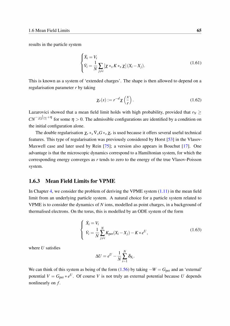
1.6 Mean Field Limits 65
results in the particle systemXi =Vi
Vi =1N ∑
j =i[χ ∗x K ∗x χ] (Xi −X j).
(1.61)
This is known as a system of ‘extended charges’. The shape is then allowed to depend on aregularisation parameter r by taking
χr(x) := r−dχ
(xr
). (1.62)
Lazarovici showed that a mean field limit holds with high probability, provided that rN ≥CN− 1
d(d+2)+η for some η > 0. The admissible configurations are identified by a condition onthe initial configuration alone.
The double regularisation χr ∗x ∇xG∗x χr is used because it offers several useful technicalfeatures. This type of regularisation was previously considered by Horst [53] in the Vlasov-Maxwell case and later used by Rein [75]; a version also appears in Bouchut [17]. Oneadvantage is that the microscopic dynamics correspond to a Hamiltonian system, for which thecorresponding energy converges as r tends to zero to the energy of the true Vlasov-Poissonsystem.
1.6.3 Mean Field Limits for VPME
In Chapter 4, we consider the problem of deriving the VPME system (1.11) in the mean fieldlimit from an underlying particle system. A natural choice for a particle system related toVPME is to consider the dynamics of N ions, modelled as point charges, in a background ofthermalised electrons. On the torus, this is modelled by an ODE system of the form
Xi =Vi
Vi =1N
N
∑j =i
Kper(Xi −X j)−K ∗ eU ,(1.63)
where U satisfies
∆U = eU − 1N
N
∑i=1
δXi.
We can think of this system as being of the form (1.56) by taking −W = Gper and an ‘external’potential V = Gper ∗ eU . Of course V is not truly an external potential because U dependsnonlinearly on f .

66 Introduction
The mean field limit for VPME was proved in the one dimensional case d = 1 in [44].In higher dimensions, once again there are no results available, due to the singularity of theCoulomb interaction. Instead, we consider a regularised system. We use a regularisation basedon the approach of Lazarovici [61]. We consider a system of ‘extended ions’ represented bythe following system of ODEs:
Xi =Vi
Vi =−χr ∗∇xUr(Xi),(1.64)
where Ur satisfies
∆Ur = eUr − 1N
N
∑i=1
χr(Xi), x ∈ Td. (1.65)
We are able to derive the VPME system (1.11) from this regularised system, under a
condition on the initial data that is satisfied with high probability for rN ≥CN− 1d(d+2)+η . This
matches the rate found in Lazarovici’s result for the Vlasov-Poisson system. This result isstated below as Theorem 1.24. The proof is given in Chapter 4.
1.6.4 Derivation of Kinetic Euler Systems
In Chapter 5, we consider the derivation of the kinetic incompressible Euler and kineticisothermal Euler systems introduced in Section 1.2.3.3. Our approach is based on a combinedquasi-neutral and mean field limit. We are able to derive the KInE system from a version of(1.61) with a modified scaling. Similarly, we derive the KIsE system from a version of (1.64)with a modified scaling. These results are stated below as Theorems 1.25 and 1.26.
For the KInE system, we obtain a scaling of the form
α(N) =C(logN)κ
N,
for some κ specified in the statement of Theorem 1.25. For the KIsE system, we obtain ascaling of the form
α(N) =Clog loglogN
N.
1.7 Summary of Results 67
1.7 Summary of Results
In this section, we summarise the main results of this thesis.
1.7.1 Well-Posedness for the VPME System
In Chapter 2, we will study the well-posedness theory of the Vlasov-Poisson system withmassless electrons. We prove the existence and uniqueness of bounded density solutions forcompactly supported initial data.
The key technique is a decomposition of the electrostatic potential U . We write U in theform U = U +U , where U and U satisfy the following equations:
−∆U = ρ f −1, ∆U = eU+U −1.
Thus U is the electrostatic potential used in the classical Vlasov-Poisson system, and cantherefore be handled using known methods. The key step is to study U , in particular itsregularity and stability with respect to ρ f . This decomposition was previously considered inthe one dimensional case d = 1 in [44].
We are able to show that U is in general smoother than U , including in the higher dimen-sional cases d = 2,3. This fact allows known methods for the classical Vlasov-Poisson systemto be adapted to the VPME case. In this thesis, we demonstrate this principle in two cases. Inone case, we adapt the proof of uniqueness for bounded density solutions, due to Loeper [65],to the VPME case. We then prove the existence of bounded density solutions by adapting themethods of Batt and Rein [10].
1.7.1.1 Uniqueness
We prove a uniqueness result for solutions of the VPME system (1.11) with bounded density.This is an analogue of Loeper’s result [65, Theorem 1.2] for the Vlasov-Poisson system (1.5).
Theorem 1.21 (Uniqueness of bounded density solutions for VPME). For each i = 1,2, let fi
be a solution of (1.11) in the space C([0,T ];P(Td ×Rd)), with bounded density
supt∈[0,T ]
∥ρ[ fi]∥L∞(Td) ≤Ci,
for the same initial datum f (0) ∈ P(Td ×Rd). Then f1 = f2.
The proof of this result is given in Chapter 2, in Section 2.6. As for Loeper’s result, theproof of Theorem 1.21 is based on a stability estimate for solutions of the VPME system in

68 Introduction
W2. The key step is to prove a stability estimate for U with respect to ρ f , analogous to the oneproved for U by Loeper (Theorem 1.17).
1.7.1.2 Existence of Solutions
We prove the existence of solutions for the VPME system (1.11) with bounded density, forcompactly supported initial data.
Theorem 1.22 (Existence of solutions with bounded density). Let d = 2,3. Consider an initialdatum f0 ∈ L1 ∩L∞(Td ×Rd) with compact support in Td ×Rd . Then there exists a global intime solution ft ∈C([0,∞);P(Td ×Rd)) of (1.11) with initial data f0, which has conservedenergy and a mass density bounded locally in time:
E ME[ ft ] = E ME[ f0], ρ ft ∈ L∞loc([0,∞);L∞(Td)).
The proof of this result is given in Chapter 2, Sections 2.7–2.9. The main idea is to controlthe size of the support of the solution. This is the method used by Pfaffelmoser [74], Schaeffer[79] and Batt–Rein [10] for the classical Vlasov-Poisson system. Since we work with theVPME system posed on the torus, we follow the methods of Batt and Rein [10]. The key stepis to prove suitable bounds on E =−∇U , the smooth part of the electric field.
1.7.2 Quasi-Neutral Limit for VPME With Rough Data
In Chapter 3, we prove the quasi-neutral limit from the VPME system (1.11) to the KIsEsystem (1.20), for a class of rough data. The starting point is analogous to the approach ofHan-Kwan and Iacobelli [43] for the classical Vlasov-Poisson system, which we describedin Section 1.5.4.2. The idea is to work with initial data for the VPME system that are smallperturbations of analytic functions satisfying the assumptions of Theorem 1.20.
Iterated Exponentials. In the following statement, we will use the notation expn to denotethe n-fold iteration of the exponential function. For example
exp3(x) := expexpexp(x).
Theorem 1.23 (Quasi-neutral limit). Let d = 2,3. Consider initial data fε(0) satisfying thefollowing conditions:
1.7 Summary of Results 69
• (Uniform bounds) fε(0) is bounded and has bounded energy, uniformly with respect to ε:for some constant C0 > 0,
∥ fε(0)∥L∞(Td×Rd) ≤C0 (1.66)
and12
∫Td×Rd
|v|2 f dxdv+ε2
2
∫Td
|∇U |2 dx+∫Td
UeU dx ≤C0.
• (Control of support) There exists C1 > 0 such that
fε(0,x,v) = 0 for |v|> exp(C1ε−2). (1.67)
• (Perturbation of an analytic function) There exist gε(0) satisfying, for some δ > 1, η > 0,and C > 0,
supε>0
supv∈Rd
(1+ |v|d+1)∥gε(0, ·,v)∥Bδ≤C,
supε>0
∥∥∥∥∫Rdgε(0, ·,v)dv−1
∥∥∥∥Bδ
≤ η ,
as well as the support condition (1.67), such that, for all ε > 0,
W2( fε(0),gε(0))≤[
exp4(Cε−2)]−1
for C sufficiently large with respect to C0,C1.
• (Convergence of data) gε(0) has a limit g(0) in the sense of distributions as ε → 0.
Let fε denote the unique solution of (3.1) with bounded density and initial datum fε(0). Thenthere exists a time horizon T∗ > 0, independent of ε but depending on the collection g0,εε ,and a solution g of (3.2) on the time interval [0,T∗] with initial datum g(0), such that
limε→0
supt∈[0,T∗]
W1( fε(t),g(t)) = 0.
The proof of this result is given in Chapter 3. The main idea is to develop a version of theW2 stability estimate for the VPME system that is quantified with respect to the Debye length ε .This estimate is proved in Section 3.3. This estimate is used to control the distance between thesolution fε with rough data and the analytic solution with data gε(0), which is already knownto converge in the limit ε → 0 due to Theorem 1.20.
70 Introduction
1.7.3 Derivation of VPME from a System of Extended Ions
In Chapter 4, we consider the derivation of the VPME system from an underlying microscopicsystem. We use the ‘extended ions’ system (1.64)-(1.25) introduced in Section 1.6.3. Our mainresult is the following theorem.
Theorem 1.24 (Regularised mean field limit). Let d = 2,3, and let f (0) ∈ L1 ∩L∞(Td ×Rd)
be a compactly supported choice of initial datum for (4.2). Let f denote the unique boundeddensity solution of the VPME system (1.11) with initial datum f (0).´ Fix T∗ > 0.
Assume that r = r(N) and the initial configurations for (1.64)-(1.65) are chosen suchthat the corresponding empirical measures satisfy, for some sufficiently large constant C > 0,depending on T∗ and the support of f (0),
limsupN→∞
W 22 ( f (0),µN
r (0))
rd+2+C| logr|−1/2 < 1.
Then the empirical measure µNr associated to the particle system dynamics starting from this
configuration converges to f :
limN→∞
supt∈[0,T∗]
W2( f (t),µNr (t)) = 0. (1.68)
In particular, suppose that f0 has a finite kth moment for some k > 4:∫Td×Rd
(|x|k + |v|k
)f0(dxdv)<+∞.
Choose r(N) = N−γ for some γ satisfying
γ <1
d +2min
1d,1− 4
k
.
For each N, let the initial configurations for the regularised N-particle system (4.4) be chosenby taking N independent samples from f0. Then (1.68) holds with probability one.
1.7.4 Derivation of Kinetic Euler Systems from Systems of ExtendedCharges
In Chapter 5, we derive the KInE (1.16) and KIsE (1.20) systems from underlying microscopicsystems of extended charges.
1.7 Summary of Results 71
1.7.4.1 Kinetic Isothermal Euler
For the KIsE system, we consider the following system of extended ions, which is a version of(1.64)-(1.65) with quasi-neutral scaling:
Xi =Vi
Vi =−χr ∗∇xU(Xi),(1.69)
where U satisfies
ε2∆U = eU − 1
N
N
∑i=1
χr(x−Xi).
Recall that χr is the scaled mollifier defined in (1.62). For this system, we prove the followingconvergence result. We state the result here for the case where the initial data for (1.69) arechosen randomly, by taking independent samples from a given law fε(0). See Theorem 5.3 inChapter 5, Subsection 5.2.2 for a statement dealing with other initial configurations.
Theorem 1.25 (From extended ions to kinetic isothermal Euler). Let d = 2 or 3, and letfε(0),gε(0) and g(0) satisfy the assumptions of Theorem 1.23. Let T∗ > 0 be the maximal timeof convergence from Theorem 1.23 and let g denote the solution of the KIsE system (5.5) withinitial data g(0) on the time interval [0,T∗] appearing in the conclusion of Theorem 1.23.
Let r = r(N) be of the form
r(N) = cN− 1d(d+2)+η
, for some η > 0, c > 0.
There exists a constant C, depending on d, η , c and fε(0)ε , such that the following holds.Let ε = ε(N) satisfy
ε(N)≥ C√log loglogN
, limN→∞
ε(N) = 0.
For each N, let the initial conditions for the regularised and scaled N-particle ODE system(1.69) be chosen randomly with law fε(N)(0)⊗N . Let µN
ε,r(t) denote the empirical measureassociated to the solution of (1.69).
Then, with probability one,
limN→∞
supt∈[0,T∗]
W1(µ
Nε,r(t),g(t)
)= 0.

72 Introduction
1.7.4.2 Kinetic Incompressible Euler
We also prove a similar result for the KInE system. For the microscopic model, we considerthe following system of extended electrons:
Xi =Vi
Vi =ε−2
N ∑j =i
χr ∗Kper ∗χr(Xi −X j).
In this case, we choose configurations for the particle system that approximate initial datafε(0) for the Vlasov-Poisson system (1.5) for which the quasi-neutral limit holds. Specifically,we assume that fε(0) satisfy the assumptions of the rough data result of Han-Kwan–Iacobelli[43]. These assumptions are stated below.
Assumption 1 (KInE, d = 2,3). The data fε(0) satisfy the following:
(i) There exists C0 independent of ε such that
∥ fε(0)∥L∞ ≤C0, E VPε ( fε(0))≤C0.
(ii) (Control of support) For some γ > 0,
fε(0,x,v) = 0 for |v|> ε−γ . (1.70)
(iii) (Analytic + perturbation) There exist functions gε(0) satisfying (1.70) and
supε∈(0,1)
supv∈Rd
(1+ |v|d+1)∥gε(0, ·,v)∥Bδ0≤C,
such thatW2( fε(0),gε(0))≤
[exp2
(Cε
−(2+dζ ))]−1
,
for C > 0 sufficiently large, where ζ = ζ (γ) is defined as follows:
• For d = 2, we fix any δ > 2 and let
ζ = maxγ,δ.
• For d = 3 we let
ζ = max
γ,383
.
1.7 Summary of Results 73
We then have the following result.
Theorem 1.26. Let d = 2 or 3. For each ε > 0, let fε(0) satisfy Assumption 1. Suppose thatgε(0) has a limit g(0) in the sense of distributions as ε tends to zero. There exists T∗ > 0 and asolution g(t) of (1.16) on the time interval [0,T∗] such that the following holds.
Fix T ≤ T∗ and α > 0. There exist constants AT , CT depending on T , α and fε(0)ε suchthat the following holds. Let r = r(N), ε = ε(N) satisfy
r = AT N− 1d(d+2)+α
, ε ≥CT (logN)− 1
2+dζ
Then, if the initial N-particle configurations [Zεi (0)]
Ni=1 are chosen by taking N independent
samples from fε(0), with probability one the following limit holds:
limN→∞
supt∈[0,T ]
W1(µNε,r(t),g(t)) = 0,
where
• µNε,r(t) denotes the empirical measure corresponding to the solution of (5.4) with initial
datum [Zεi (0)]
Ni=1 ;
• µNε,r(t) is the measure constructed by filtering µN
ε,r(t) using the corrector Rε defined in(1.53), according to Definition 5 in Chapter 5, Subsection 5.2.1.1, using the given choiceof fε(0) and g(0).

Chapter 2
The Vlasov-Poisson System with MasslessElectronsGlobal Well-posedness in Two and Three Dimensions
Contents2.1 Statement of Results . . . . . . . . . . . . . . . . . . . . . . . . . . . . . 77
2.1.1 Uniqueness of Solutions With Bounded Density . . . . . . . . . . . 77
2.1.2 Global Existence of Solutions . . . . . . . . . . . . . . . . . . . . 77
2.2 Strategy . . . . . . . . . . . . . . . . . . . . . . . . . . . . . . . . . . . . 78
2.3 Basic Estimates . . . . . . . . . . . . . . . . . . . . . . . . . . . . . . . . 79
2.3.1 Lp(Td ×Rd) Estimates . . . . . . . . . . . . . . . . . . . . . . . . 79
2.3.2 Energy . . . . . . . . . . . . . . . . . . . . . . . . . . . . . . . . 79
2.3.3 Estimates on the Mass Density . . . . . . . . . . . . . . . . . . . . 80
2.4 Regularity of the Electric Field . . . . . . . . . . . . . . . . . . . . . . . 81
2.4.1 Regularity of U . . . . . . . . . . . . . . . . . . . . . . . . . . . . 82
2.4.2 Existence of U . . . . . . . . . . . . . . . . . . . . . . . . . . . . 83
2.4.3 Regularity of U . . . . . . . . . . . . . . . . . . . . . . . . . . . . 87
2.5 Stability of the Electric Field . . . . . . . . . . . . . . . . . . . . . . . . 90
2.6 Wasserstein Stability and Uniqueness . . . . . . . . . . . . . . . . . . . 93
2.7 A Priori Estimates on the Mass Density . . . . . . . . . . . . . . . . . . 101
2.7.1 Two-dimensional Case . . . . . . . . . . . . . . . . . . . . . . . . 101
76 VPME: Global Well-posedness in 2D and 3D
2.7.2 Three-dimensional Case . . . . . . . . . . . . . . . . . . . . . . . 105
2.8 A Regularised System . . . . . . . . . . . . . . . . . . . . . . . . . . . . 110
2.9 Construction of Solutions . . . . . . . . . . . . . . . . . . . . . . . . . . 114
2.9.1 Energy conservation . . . . . . . . . . . . . . . . . . . . . . . . . 131
In this chapter, we prove global-in-time well-posedness results for the Vlasov-Poissonsystem with massless electrons (VPME) in dimension d = 2,3. Recall that VPME is a kineticmodel for the ions in a plasma. We introduced this model from a physical perspective inSection 1.2.2. On the torus, the system reads as follows:
(V PME) :=
∂t f + v ·∇x f +E ·∇v f = 0,E =−∇xU,
∆xU = eU −∫Rd
f dv = eU −ρ f ,
f |t=0 = f (0)≥ 0,∫Td×Rd
f (0,x,v)dxdv = 1.
(2.1)
Global well-posedness of the VPME system was shown in the one dimensional case in Han-Kwan–Iacobelli [43]. In three dimensions, Bouchut [17] proved the global-in-time existence ofweak solutions. However, global existence of strong solutions was not proved in dimensionshigher than one.
In this chapter, we prove global-in-time existence of strong solutions of the VPME systemin dimensions d = 2 and d = 3, for compactly supported data. We also prove the uniqueness ofsolutions with bounded density.
These results provide analogues of two important results for the classical Vlasov-Poissonsystem (1.5). Our uniqueness result is comparable to the result of Loeper [65] for the classicalsystem. We also prove a global existence result in the style of Batt and Rein [10] for solutionson the torus for d = 2,3.
The key step in our analysis is a decomposition of the electric field. We are able to showthat the electric field in the VPME system behaves like a perturbation of the electric field inthe classical Vlasov-Poisson system (1.5). This perturbation is general more regular than theremainder of the electric field. This key observation allows known methods for the classicalsystem to be adapted to the VPME case. We demonstrate this in full for the results mentionedabove.
2.1 Statement of Results 77
2.1 Statement of Results
The aim of this chapter is to prove the following results. Together they provide, for d = 2,3,global existence of solutions of the VPME system (2.1), for a general class of data, as well asuniqueness for solutions with bounded density.
2.1.1 Uniqueness of Solutions With Bounded Density
Theorem 2.1 (Uniqueness for solutions with bounded density). Let d = 2,3. Let f0 ∈ P(Td ×Rd)
with ρ[ f0]∈L∞(Td). Fix a final time T > 0. Then there exists at most one solution f ∈C([0,T ];P(Td ×Rd))
of the system (2.1), with initial datum f0, such that ρ[ f ] ∈ L∞([0,T ];L∞(Td)).Moreover, we have a quantitative stability estimate. Let f ,g be solutions of the VPME
system (2.1) such that
supt∈[0,T ]
∥ρ[ f (t)]∥L∞(Td), supt∈[0,T ]
∥ρ[g(t)]∥L∞(Td) ≤ M
for some constant M > 0. Then there exists C > 0 depending on M such that for all t ∈ [0,T ],
W2( f (t),g(t))≤
exp[C(
1+ log W2( f (0),g(0))4√
d
)e−Ct
]if W2( f (0),g(0))≤ d
W2( f (0),g(0))eCt if W2( f (0),g(0))> d.
The proof of this theorem is given in Section 2.6.
2.1.2 Global Existence of Solutions
We prove a result of global-in-time existence, analogous to that of Batt and Rein [10] for theVlasov-Poisson system (1.5). The following theorem is proved in Sections 2.7 and 2.9.
Theorem 2.2 (Existence of solutions with bounded density). Let d = 2,3. Consider an initialdatum f0 ∈ L1 ∩L∞(Td ×Rd) with compact support in Td ×Rd . Then there exists a globalin time solution f ∈ C([0,∞);P(Td ×Rd)) of (1.11) with initial data f0. This solution hasbounded density, locally in time:
ρ f ∈ L∞loc([0,∞);L∞(Td)).
78 VPME: Global Well-posedness in 2D and 3D
2.2 Strategy
The core of this chapter is an analysis of the electric field E in the VPME system, which iscarried out in Sections 2.4 and 2.5. We prove integrability and regularity estimates on E interms of integrability estimates on ρ f , as well as estimates on the stability of E with respect toρ f . We have discussed in Sections 1.3 and 1.4 that this is the key information needed whenstudying well-posedness for a nonlinear equation of Vlasov type.
The fundamental step in our analysis is a decomposition of E. For example, in the toruscase we write E as E + E where
E =−∇U , E =−∇U ,
and U and U solve respectively
∆U = 1−ρ f , ∆U = eU+U −1.
This decomposition was previously used in [44] for the one dimensional case.The advantage of this decomposition is that it allows us to think of E as a perturbation of
the electric field E that we would have in the classical Vlasov-Poisson system (1.5). Moreover,the perturbation E depends on ρ f only through U , which will be smoother than ρ f due to theregularising properties of the Poisson equation. We might therefore expect U to have higherorder regularity than U , and this is indeed what we find (see Proposition 2.4). For this reason wesometimes refer to U as the ‘singular’ part of the potential, and U as the ‘regular’ or ‘smooth’part.
The challenging part of the analysis of U is that it satisfies an equation with an exponentialnonlinearity. It turns out that, even though the nonlinearity is exponential, it has a helpful signwhich allows it to be controlled. We show this using techniques from Calculus of Variations.This strategy was also used in the one-dimensional case in [44]. Here we are able to extendthese results to higher dimensions.
These regularity estimates allow us to adapt methods developed for the classical Vlasov-Poisson system to the VPME case. In Section 2.6, we prove Theorem 2.1 on the uniqueness ofbounded density solutions. The strategy is to prove a W2 stability estimate on solutions, withrespect to their initial data. This proof follows the strategy of Loeper [65].
In Section 2.9, we construct global-in-time solutions of the VPME system on the torus(2.1). Our approach follows the method of Batt and Rein [10] for the classical Vlasov-Poissonsystem, which is in itself an adaptation of the methods of Pfaffelmoser [74] and Schaeffer [79]to the torus. The key step is to control the growth of the size of the support of ft in Td ×Rd .
2.3 Basic Estimates 79
In Section 2.8, we prove the existence of unique solutions to a regularised version ofthe VPME system. This will allow us to complete the existence proof by an approximationargument. This result is not quite covered in the existing literature to our knowledge, becausethe electric field E in the VPME system cannot be written in the form
E = F ∗ρ
for some F . Instead, the coupling between E and ρ is nonlinear. However, the estimates inSections 2.4 and 2.5 allow us to adapt well-known methods for Vlasov equations with smoothinteractions, which we presented in Section 1.3, to our approximating system.
2.3 Basic Estimates
In this section, we summarise some basic estimates for solutions of the VPME system. Ina similar spirit to Section 1.4.1, we look at the a priori estimates we can expect to have onsolutions, based on the conservation laws of the system.
2.3.1 Lp(Td ×Rd) Estimates
Solutions f of the VPME system solve a transport equation with a divergence free vector field.If f0 ∈ L1 ∩L∞(Td ×Rd), we therefore have uniform in time estimates on the Lp(Td ×Rd)
norms of f .
Lemma 2.3. Assume that f0 ∈ L1 ∩L∞(Td ×Rd). Let f be a solution of (2.1). Then, for allp ∈ [1,∞],
∥ ft∥Lp(Td×Rd) ≤ ∥ f0∥1p
L1(Td×Rd)∥ f0∥
1− 1p
L∞(Td×Rd).
2.3.2 Energy
The system (2.1) has an associated energy functional:
E ME[ f ] :=12
∫Td×Rd
|v|2 f dxdv+12
∫Td
|∇U |2 dx+∫Td
UeU dx. (2.2)
This functional is conserved by the evolution for smooth solutions.The conservation of the energy functional provides a uniform estimate on the second
moment of f in velocity, or, in other words, the kinetic energy of f . In Section 1.4.1, wediscussed a similar property for the classical Vlasov-Poisson system. For the classical system

80 VPME: Global Well-posedness in 2D and 3D
(1.5) this implication is immediate because both terms in the classical energy (1.46) are non-negative.
For the VPME energy functional (2.2), we need to deal with the fact that some of the termsmay be negative. In particular, we need to consider possible values of the function x 7→ xex forx ∈ R. Since
ddx
(xex) = (x+1)ex,
it follows that, for all x ∈ R,xex ≥ (xex)|x=−1 =−e−1.
Consequently, bounds on the total energy E ME imply bounds on the kinetic energy:
12
∫Td×Rd
|v|2 f dxdv ≤ E ME[ f ]+ e−1. (2.3)
2.3.3 Estimates on the Mass Density
As discussed in Section 1.4.1, it is possible to deduce Lp(Td) estimates on the mass densityρ f from estimates on the moments of the full phase-space density f . Using the bound (2.3)on the kinetic energy, we can therefore obtain the same L
d+2d (Td) estimate on ρ f as in the
classical case, using the interpolation estimate from Lemma 1.12. Since the energy functionalsare formally conserved by their respective equations, this estimate is uniform in time. That is,we can expect a uniform bound of the form
∥ρ f (t, ·)∥L
d+2d (Td)
≤C(d, f0). (2.4)
The constant C( f0) depends on the initial datum f0 through the relation
C(d, f0) =Cd(E ME[ f0]+ e−1) d
d+2 ∥ f0∥2
d+2L∞(Td×Rd)
,
where Cd is a dimension dependent constant.In the next section, we will derive regularity estimates on the electric field in terms of
integrability estimates on ρ f . The crucial point is that we will be able to derive estimates onthe smooth part of the potential U that depend on the L
d+2d (Td) norm of ρ f , and are therefore
uniform in time.
2.4 Regularity of the Electric Field 81
2.4 Regularity of the Electric Field
In this section we prove several key regularity estimates on the electric field in the VPMEsystem. These estimates will ultimately show that the electric field in the VPME case is asmooth perturbation of the field in the classical case. This fact will allow us to adapt the existingtechniques for proving well-posedness of the Vlasov-Poisson system to the massless electronmodel.
The strategy is based on the following decomposition of the electric field. We let E = E+ E,where
E =−∇U , E =−∇U ,
and U and U solve respectively
∆U = 1−ρ f , ∆U = eU+U −1.
We impose without loss of generality that U has zero mean over the torus:∫Td
U dx = 0.
Notice that in this way U := U +U solves
∆U = eU −ρ f .
We consider charge densities ρ f ∈ L∞(Td), since the solutions of VPME we will work withwill have densities in this class. We want to derive integrability and regularity estimates onE, assuming that ρ f has this degree of integrability. In particular, the aim is to give estimatesin terms of the L
d+2d (Td) and L∞(Td) norms of ρ f . The L
d+2d (Td) norm is of interest because
the conservation of energy for the VPME system provides a uniform-in-time bound on thisquantity.
Our aim is to prove the following proposition.
Proposition 2.4 (Regularity estimates on U and U). Let d = 2,3. Let h ∈ L∞(Td). Then thereexist unique U ∈W 1,2(Td) with zero mean and U ∈W 1,2(Td) satisfying
∆U = 1−h, ∆U = eU+U −1.
82 VPME: Global Well-posedness in 2D and 3D
Moreover we have the following estimates: for some constant Cα,d > 0,
∥U∥C0,α (Td) ≤Cα,d
(1+∥h∥
Ld+2
d (Td)
), α ∈
(0,1) if d = 2
(0, 15 ] if d = 3.
∥U∥C1,α (Td) ≤Cα,d
(1+∥h∥L∞(Td)
), α ∈ (0,1)
∥U∥C1,α (Td) ≤Cα,d exp(
Cα,d
(1+∥h∥
Ld+2
d (Td)
)), α ∈ (0,1)
∥U∥C2,α (Td) ≤Cα,d exp exp(
Cα,d
(1+∥h∥
Ld+2
d (Td)
)), α ∈
(0,1) if d = 2
(0, 15 ] if d = 3.
.
The remainder of this section is structured as follows:
(i) In Section 2.4.1, we discuss the existence and regularity of U , which is based on standardtheory for the Poisson equation.
(ii) In Section 2.4.2, we prove the existence of U , given U with the regularity derived above.Our proof uses techniques from the calculus of variations.
(iii) In Section 2.4.3, we prove energy estimates on U . These estimates imply regularity for Uusing the regularity theory of the Poisson equation.
2.4.1 Regularity of U
The regularity estimates on U are based on the analysis of the following Poisson equation
∆U = 1−h.
The existence of a solution U ∈W 1,2(Td), unique up to additive constants, for h ∈ L2(Td)⊃L∞(Td) is well-known - see for example [28, Chapter 6]. Choosing a solution with zero meanthen specifies U uniquely. In the following lemma, we recall some standard elliptic regularityestimates for this solution, that follow from Calderón-Zygmund estimates for the Laplacian[30, Section 9.4], and Sobolev inequalities.
Lemma 2.5. Let U ∈W 1,2(Td) have zero mean and satisfy
∆U = h.
2.4 Regularity of the Electric Field 83
(i) If h ∈ Ld+2
d (Td), then for all α ∈ (0,1), if d = 2, or α ∈ (0, 15 ] if d = 3, there exists a
constant Cα,d > 0 such that
∥U∥C0,α (Td) ≤Cα,d
(1+∥h∥
Ld+2
d (Td)
).
(ii) If h ∈ L∞(Td), then for any α ∈ (0,1), there exists a constant Cα,d such that
∥U∥C1,α (Td) ≤Cα,d ∥h∥L∞(Td).
In order to prove estimates on the VPME system, we would ideally like to have goodcontrol of the regularity of the electric field, especially the singular part ∇U . The estimates inLemma 2.5 are not quite strong enough to provide Lipschitz regularity for ∇U . However, alog-Lipschitz estimate is available. We stated this as Lemma 1.11 in the introduction and gavea proof there. Below, we recall the statement.
Lemma 2.6 (Log-Lipschitz regularity of E). Let U be a solution of
∆U = h
for h ∈ L∞(Td). Then
|∇U(x)−∇U(y)| ≤Cd∥h∥L∞(Td)|x− y|
(1+ log
( √d
|x− y|
)1|x−y|≤
√d
).
2.4.2 Existence of U
In this section we prove the existence of a solution U of the equation
∆U = eU+U −1, (2.5)
under the condition that U ∈ W 1,2∩L∞(Td). By Lemma 2.5, when we consider solutions of theVPME system (2.1), we expect U to have this regularity. Our strategy is to seek a minimiser ofthe functional
h 7→ J [h] :=∫Td
12|∇h|2 +
(eU+h −h
)dx
in the space h ∈ W 1,2(Td). We then use the fact that equation (2.5) is the Euler-Lagrangeequation of this minimisation problem to conclude that the minimiser is a solution of (2.5).
The following lemma holds in any dimension d.

84 VPME: Global Well-posedness in 2D and 3D
Lemma 2.7 (Existence of a Unique Minimiser). Let U ∈ W 1,2 ∩L∞(Td). Then there exists aunique U ∈W 1,2(Td) such that
J [U ] = infh∈W 1,2(Td)
J [h].
Proof. The uniqueness of minimisers follows from the fact that J is a strictly convex func-tional.
We prove existence of a minimiser using the direct method of the calculus of variations.Consider a minimising sequence (hk)k∈N such that, as k tends to infinity,
J [hk]→ infh∈W 1,2(Td)
J [h].
We will show that hk is uniformly bounded in W 1,2(Td). This will allow us to extract aconvergent subsequence. Since U ∈ W 1,2 ∩L∞(Td) and the torus has finite measure, in factU ∈W 1,2(Td) by monotonicity of Lp norms. Therefore, for k sufficiently large,
J [hk]≤ J [−U ]
= ∥∇U∥2L2(Td)+
∫Td(1+U)dx
≤ ∥∇U∥2L2(Td)+1+∥U∥L∞(Td) =: C1. (2.6)
The constant C1 is finite since U ∈ W 1,2 ∩L∞(Td).We observe that
eU+s − s = eU es − s ≥ e−∥U∥L∞(Td )es − s ≥ s2 −C2,
for some constant C2 depending on ∥U∥L∞(Td) only. Thus
∫Td
eU+hk −hk dx ≥∫Td
h2k −C2 dx. (2.7)
By equations (2.6) and (2.7),∫Td
12|∇hk|2 +(h2
k −C2)dx ≤ J [hk]≤C1 +1.
Thus the sequence (hk)k∈N is bounded in W 1,2(Td), uniformly in k:
||∇hk||L2(Td)+ ||hk||L2(Td) ≤C3,

2.4 Regularity of the Electric Field 85
where the constant C3 is independent of k.By weak compactness of W 1,2(Td), up to a subsequence hk converges weakly in W 1,2(Td)
to a function U :hkU in W 1,2(Td).
Since W 1,2(Td) is compactly embedded in L2(Td), we also have strong convergence:
hk→U in L2(Td).
Then, up to a further subsequence, we have
hk → U a.e.
To show that U is indeed a minimiser, we prove that J is lower semicontinuous. By theweak convergence of hk to U in W 1,2(Td) and by strong convergence in L2(Td),
liminfk→∞
∫Td
12|∇hk|2 dx ≥
∫Td
12|∇U |2 dx,
since the norm is lower semicontinuous under weak convergence. Strong convergence inL2(Td) implies strong convergence in L1(Td)), and therefore
limk→∞
∫Td
hk dx =∫Td
U dx.
By Fatou’s Lemma,
liminfk→∞
∫Td
eU+hk dx ≥∫Td
liminfk→∞
eU+hk dx =∫Td
eU+U dx.
We conclude thatlimk→∞
J [hk]≥ J [U ],
which proves that U is a minimiser.
Next, we check that the minimiser U solves the Euler-Lagrange equation (2.5). Again thisholds in any dimension d.
Lemma 2.8 (Euler-Lagrange Equation). Let U ∈ W 1,2 ∩L∞(Td) and let U ∈W 1,2(Td) be theunique minimiser of J whose existence was proved in Lemma 2.7. Then U is a weak solutionof equation (2.5).
86 VPME: Global Well-posedness in 2D and 3D
Proof. First observe that, by definition of a minimiser,
J [U ]≤ J [−U ]<+∞.
Explicitly, by definition of J ,∫Td
12|∇U |2 +
(eU eU −U
)dx ≤ J [−U ]<+∞.
Since U ∈W 1,2(Td), by monotonicity of norms on the torus we have U ∈ L1(Td). From thiswe deduce that ∫
TdeU eU dx <+∞.
Since ∥U∥L∞(Td) is finite, it follows that
∫Td
eU dx <+∞.
Altogether, we have ∇U ∈ L2(Td), U ∈ L1(Td), eU ∈ L∞(Td), and eU ∈ L1(Td).
We now show that U is a weak solution of (2.5). Let φ ∈C∞c ,η > 0. By minimality of U ,
J [U ]≤ J [U +ηφ ].
Then,
0 ≤ J [U +ηφ ]−J [U ]
η=
1η
(∫Td
12|∇U +η∇φ |2 − 1
2|∇U |2 dx
)+
1η
(∫Td
eU eU+ηφ − eU eU dx)+
1η
(∫Td
−(U +ηφ)+U dx)
=∫Td
∇U ·∇φ +η |∇φ |2
2dx+
∫Td
eU+U eηφ −1η
dx−∫Td
φ dx.
In the limit as η goes to 0 we obtain, for all φ ∈C∞c (Td),
0 ≤ limη→0
J [U +ηφ ]−J [U ]
η=∫Td
∇U ·∇φ dx+∫Td
eU+Uφ dx−
∫Td
φ dx.
2.4 Regularity of the Electric Field 87
Since the latter inequality is valid both for φ and for −φ , we have that, for all φ ∈C∞c (Td),
0 =∫Td
∇U ·∇φ +(
eU+U −1)
φ dx. (2.8)
This implies that U is a weak solution of the equation
∆U = eU+U −1 on Td,
which completes the proof.
2.4.3 Regularity of U
In this section, we prove regularity estimates on U .
Lemma 2.9 (Regularity of U). (i) Let U ∈ W 1,2 ∩L∞(Td), with the estimate
∥U∥L∞(Td) ≤ M1.
Let U ∈W 1,2(Td) be the solution of (2.5) constructed in Section 2.4.2. Then U ∈C1,α(Td)
for any α ∈ (0,1), with the estimate
∥U∥C1,α (Td) ≤C(1+ e2M1
).
(ii) Let U ∈ W 1,2 ∩C0,α(Td) for some α ∈ (0,1), with the estimate
∥U∥C0,α (Td) ≤ M2.
Then U ∈C2,α(Td) with
∥U∥C2,α (Td) ≤C exp[C(M1 +(1+ e2M1)
)](M2 +(1+ e2M1)
).
Proof. Our general strategy will be to consider the equation satisfied by U :
∆U = eU+U −1, (2.9)
which we think of as a Poisson equation with source eU+U − 1. The aim is to make use ofstandard regularity estimates for the Poisson equation in order to deduce the required regularityfor U . The first part of the statement follows from Calderón-Zygmund estimates and Sobolevembedding, while the second part makes use of Schauder estimates. However, in order to

88 VPME: Global Well-posedness in 2D and 3D
implement this strategy, we must first prove suitable Lp and Hölder estimates on the sourceterm eU+U −1. We will obtain these using energy estimates on the equation (2.9).
To prove an Lp estimate on eU+U for p > 1, the formal argument is to choose e(p−1)U as atest function in the weak form of equation (2.9). Since
∇e(p−1)U = (p−1)e(p−1)U∇U ,
from (2.9) we obtain
−(p−1)∫Td
|∇U |2e(p−1)U dx =∫Td
(eU epU − e(p−1)U
)dx.
This implies that ∫Td
eU epU dx ≤∫Td
e(p−1)U dx.
Bounding eU from below using the L∞ norm of U , we obtain
e−M1
∫Td
epU dx ≤∫Td
e(p−1)U dx.
In other words,∥eU∥p
Lp(Td)≤ eM1∥eU∥p−1
Lp−1(Td). (2.10)
To this we add an L1(Td) estimate, which follows from the fact that eU −1 must have totalintegral zero: since U is a solution of (2.5), we have
0 =∫Td
∆U dx =∫Td
eU −1dx.
Since U = U +U , it follows that
1 =∫Td
eU+U dx ≥ e−M1
∫Td
eU dx.
Thus∥eU∥L1(Td) =
∫Td
eU dx ≤ eM1.
Applying (2.10) in the case p = 2, we find that
∥eU∥L2(Td) ≤ eM1.
By induction we then obtain∥eU∥Ln(Td) ≤ eM1 (2.11)

2.4 Regularity of the Electric Field 89
for any integer n.We now check that (2.10) can be obtained rigorously. The weak form of equation (2.9)
is given in equation (2.8); that is, U satisfies (2.8) for test functions φ ∈ C∞(Td). SinceeU ∈ L1(Td), this further extends to all φ ∈ L∞∩W 1,2(Td) by a density argument. We thereforedefine a test function in L∞ ∩W 1,2(Td) that approximates e(p−1)U .
Consider the truncated function
Uk := (U ∧ k), for allk ∈ N.
Since e(p−1)Uk ∈ L∞(Td) and ∇U ∈ L2(Td),
∇e(p−1)Uk = (p−1)e(p−1)Uk∇Uk = (p−1)eUk∇UχU<k ∈ L2(Td);
thus e(p−1)Uk ∈ L∞ ∩W 1,2(Td), and we can use it as a test function in equation (2.8):
0 =∫Td
∇U ·∇e(p−1)Uk dx+∫Td
(eU e(U+(p−1)Uk)− e(p−1)Uk
)dx
= (p−1)∫Td
∇U · e(p−1)Uk∇UχU<k dx+∫Td
(eU e(U+(p−1)Uk)− e(p−1)Uk
)dx
= (p−1)∫Td
|∇U |2e(p−1)Uk χU<k dx+∫Td
eU e(U+(p−1)Uk) dx−∫Td
e(p−1)Uk dx.(2.12)
Since∫Td |∇U |2e(p−1)Uk χU<k dx ≥ 0, and e−M1 ≤ eU ≤ eM1 , (2.12) implies that
e−M1
∫Td
eU+(p−1)Uk ≤∫Td
e(p−1)Uk .
By definition of Uk we have that e(p−1)Uk is increasing and converges monotonically to e(p−1)U ,hence by the Monotone Convergence Theorem
e−M1
∫Td
eU+(p−1)U = e−M1
∫Td
epU ≤∫Td
eU .
Thus we obtain (2.10), which implies the Ln estimate (2.11) for any integer n.We now prove the desired estimates on U . For part (i) of the statement, we apply (2.11) for
some n > d. Since
∥eU∥Ln(Td) = ∥eU+U∥Ln(Td) ≤ e∥U∥L∞(Td )∥eU∥Ln(Td) ≤ e2M1,
we have∆U = eU+U −1 ∈ Ln(Td),
90 VPME: Global Well-posedness in 2D and 3D
with∥eU+U −1∥Ln(Td) ≤ 1+ e2M1 .
By Calderón-Zygmund estimates for the Poisson equation [30, Section 9.4],
∥U∥W 2,n(Td) ≤Cn,d(1+ e2M1
).
Using Sobolev embedding for n sufficiently large, we deduce that for any α ∈ (0,1), U ∈C1,α(Td), with
∥U∥C1,α (Td) ≤Cα,d(1+ e2M1
).
For part (ii) of the statement, it is enough to prove a bound on the C0,α(Td) norm of U .This bound is provided by part (ii). Then, if
∥U∥C0,α (Td) ≤ M2,
we have∥U∥C0,α (Td) ≤ M2 +Cα,d
(1+ e2M1
),
and so∥eU∥C0,α (Td) ≤C exp
[C(M1 +
(1+ e2M1
))](M2 +
(1+ e2M1
)).
Thus ∆U ∈C0,α(Td).We may then apply Schauder estimates [30, Chapter 4] to obtain U ∈C2,α with the following
estimate:
∥U∥C2,α (Td) ≤C(∥U∥L∞(Td)+∥eU −1∥C0,α (Td)
)≤C exp
[C(M1 +
(1+ e2M1
))](M2 +
(1+ eM1
)).
This completes the proof of part (ii).
2.5 Stability of the Electric Field
In this section we study the stability of the electric field E =−∇U with respect to the chargedensity ρ f . This is one of the key estimates needed to prove the uniqueness of solutions withbounded density. Our aim is to prove a version of the following estimate for the singular part E,due to Loeper [65].

2.5 Stability of the Electric Field 91
Lemma 2.10 (Loeper-type estimate for Poisson’s equation). For each i = 1,2, let hi ∈ L∞(Td)
be a probability density function:
hi ≥ 0,∫Td
hi(x)dx = 1.
Let Ui be a solution of∆Ui = hi −1.
Then∥∇U1 −∇U2∥2
L2(Td) ≤ maxi
∥hi∥L∞(Td)W22 (h1,h2).
The main result of this section is the following proposition:
Proposition 2.11. For each i = 1,2, let Ui be a solution of
∆Ui = hi −1,
where hi ∈ L∞ ∩L(d+2)/d(Td). Then
∥∇U1 −∇U2∥2L2(Td) ≤ max
i∥hi∥L∞(Td)W
22 (h1,h2).
Now, in addition, let Ui be a solution of
∆Ui = eUi+Ui −1. (2.13)
Then
∥∇U1 −∇U2∥2L2(Td) ≤ exp exp
[Cd
(1+max
i∥hi∥L(d+2)/d(Td)
)]×max
i∥hi∥L∞(Td)W
22 (h1,h2).
Proof. We will show that
∥∇U1 −∇U2∥2L2(Td) ≤C∥U1 −U2∥2
L2(Td). (2.14)
The proposition then follows from the Poincaré inequality for zero mean functions:
∥U1 −U2∥2L2(Td) ≤Cd∥∇U1 −∇U2∥2
L2(Td).
We then apply the Loeper estimate from Lemma 2.10.
92 VPME: Global Well-posedness in 2D and 3D
We now prove (2.14). For convenience, we define the constant
A := exp[
maxi
∥Ui∥L∞(Td)+maxi
∥Ui∥L∞(Td)
]which will be fixed throughout the proof. Note that A can be controlled using Proposition 2.4,
∥Ui∥L∞(Td) ≤Cd
(1+∥hi∥
Ld+2
d (Td)
), ∥Ui∥L∞(Td) ≤ exp
(Cd
(1+∥hi∥
Ld+2
d (Td)
)).
Subtracting the two equations (2.13), we deduce that U1 −U2 satisfies
∆(U1 −U2) = eU1+U1 − eU2+U2 = eU1(
eU1 − eU2)+ eU2
(eU1 − eU2
). (2.15)
The weak form of (2.15) extends by density to test functions in L∞ ∩W 1,2(Td). SinceU1 −U2 has this regularity by assumption, it is an admissible test function. Hence
−∫Td|∇U1 −∇U2|2 dx =
∫Td
eU1(
eU1 − eU2)(U1 −U2)dx (2.16)
+∫Td
eU2(
eU1 − eU2)(U1 −U2)dx =: I1 + I2.
Observe that (ex − ey)(x− y) is always non-negative. Furthermore, by the Mean ValueTheorem applied to the function x 7→ ex we have a lower bound
(ex − ey)(x− y)≥ eminx,y(x− y)2.
We use this to bound I1 from below:
I1 ≥ e−∥U1∥L∞(Td )−maxi ∥Ui∥L∞(Td )∥U1 −U2∥2L2(Td) ≥ A−1∥U1 −U2∥2
L2(Td). (2.17)
For I2 we use the fact that, again by the Mean Value Theorem,
|ex − ey| ≤ emaxx,y|x− y|.
Therefore
I2 ≤ e∥U2∥L∞(Td )+maxi ∥Ui∥L∞(Td )
∫Td
|U1 −U2||U1 −U2|dx ≤ A∫Td
|U1 −U2||U1 −U2|dx.
2.6 Wasserstein Stability and Uniqueness 93
By the Cauchy-Schwarz inequality, for any choice of α > 0
I2 ≤ A(
α∥U1 −U2∥2L2(Td)+
14α
∥U1 −U2∥2L2(Td)
). (2.18)
Substituting (2.17) and (2.18) into (2.16), we obtain
∫Td|∇U1 −∇U2|2 dx ≤ A
(α∥U1 −U2∥2
L2(Td)+1
4α∥U1 −U2∥2
L2(Td)
)−A−1∥U1 −U2∥2
L2(Td). (2.19)
We wish to choose α as small as possible such that
A4α
−A−1 ≤ 0.
Thus the optimal choice is α = A2
4 . Substituting this into (2.19) gives
∫Td|∇U1 −∇U2|2 dx ≤ 1
4A3∥U1 −U2∥2
L2(Td).
This completes the proof of (2.14).
2.6 Wasserstein Stability and Uniqueness
In this section, we prove a quantitative stability estimate between solutions with boundeddensity. This is a version of Loeper’s [65] estimate for the classical Vlasov-Poisson system,which we recalled as Theorem 1.16.
Proposition 2.12 (Stability for solutions with bounded density). For i = 1,2, let fi be solutionsof (2.1) satisfying, for some constant M > 0 and all t ∈ [0,T ],
ρ[ fi(t)]≤ M. (2.20)
Then there exists a constant C > 0, depending on M, such that, for all t ∈ [0,T ],
W2 ( f1(t), f2(t))≤ β (t,W2 ( f1(0), f2(0))) ,
94 VPME: Global Well-posedness in 2D and 3D
where β denotes the function
β (t,x) =
16deexp[(
1+ log x16d
)e−Ct] t ≤ T0
(d ∨ x)eC(1+log16)(t−T0) t > T0,
whereT0 = inf
t > 0 : 16deexp
[(1+ log
x16d
)e−Ct
]> d.
This estimate immediately implies a uniqueness result for solutions of VPME with boundeddensity.
Corollary 2.13 (Uniqueness of solutions with bounded density). For each i = 1,2, let fi be asolution of (2.1) in the space C([0,T ];P(Td ×Rd)), with bounded density
supt∈[0,T ]
∥ρ[ fi]∥L∞(Td) ≤Ci,
for the same initial datum f (0) ∈ P(Td ×Rd). Then f1 = f2.
Proof. We will prove Proposition 2.12 by means of a Gronwall type estimate. To do this, wewill first consider the evolution of particular specially constructed couplings πt ∈Π( f1(t), f2(t)).First, observe that fi can be represented as the pushforward of the initial datum fi(0) alongthe characteristic flow associated to (2.1). That is, for each i = 1,2, given fi, consider the flowZi(t;0,z) = (Xi(t;0,z),Vi(t;0,z)) defined by the system of ODEs
Xi =Vi
Vi = Ei(Xi)
(Xi(0;0,z),Vi(0;0,z)) = z = (x,v),
(2.21)
where Ei is the electric field induced by fi:
Ei =−∇Ui, ∆Ui = eUi −ρ[ fi].
We again use the decomposition Ei = Ei + Ei. Since ρ[ fi] ∈ L∞(Td) by assumption (2.20),Lemma 2.6 implies that Ei has log-Lipschitz regularity. Since L∞(Td)⊂ L
d+2d (Td), we have
ρ[ fi] ∈ L∞ ∩Ld+2
d (Td). Thus we may apply Proposition 2.4 to deduce Lipschitz regularity ofEi. Overall this implies that Ei has log-Lipschitz regularity, which is sufficient to guarantee theexistence of a unique solution to the system (2.21). The uniqueness of the flow implies that the
2.6 Wasserstein Stability and Uniqueness 95
linear Vlasov equation
∂tg+ v ·∇xg+Ei ·∇vg = 0, g|t=0 = fi(0) (2.22)
has a unique measure-valued solution g (see for instance [1, Theorem 3.1]). This solution canbe represented as the pushforward of the initial data along the characteristic flow, as defined inDefinition 2:
gt = Z(t;0, ·)# fi(0). (2.23)
Since fi is also a solution of (2.22), and the solution is unique, it follows that g = fi. We deducethat fi has the representation (2.23). Note that here we are not yet asserting any nonlinearuniqueness, because we already fixed Ei to be the electric field corresponding to fi.
We use the representation above to construct πt . First, fix an arbitrary initial couplingπ0 ∈ Π( f1(0), f2(0)). We then build a coupling πt for which each marginal evolves along theappropriate characteristic flow. That is, we let
πt = (Z1(t;0, ·)⊗Z2(t;0, ·))# π0. (2.24)
This means that, for all φ ∈Cb((Td ×Rd)2),∫(Td×Rd)2
φ(z1,z2)dπt(z1,z2) =∫Td×Rd
φ (Z1(t;0,z1),Z2(t;0,z2)))dπ0(z1,z2). (2.25)
We now consider the quantity
D(t) :=∫(Td×Rd)
2
(|X1(t;0,z1)−X2(t;0,z2)|2 + |V1(t;0,z2)−V2(t;0,z2)|2
)dπ0(z1,z2).
(2.26)By definition (2.24) we have
D(t) =∫(Td×Rd)2
|x1 − x2|2 + |v1 − v2|2 dπt(z1,z2).
It then follows from the definition of the Wasserstein distances (Definition 4) that
W 22 ( f1(t), f2(t))≤ D(t). (2.27)
Moreover, since π0 was arbitrary, we have
W 22 ( f1(0), f2(0)) = inf
π0D(0). (2.28)
96 VPME: Global Well-posedness in 2D and 3D
We will therefore focus next on controlling the growth of D(t). This amounts to performinga Gronwall estimate along the trajectories of the characteristic flow. We give the details inLemma 2.14 below. We obtain a bound
D(t)≤ β (t,D(0)) ,
where the function β is defined by
β (t,x)≤
16deexp[(
1+ log x16d
)e−Ct] t ≤ T0(x)
(d ∨ x)eC(1+log16)(t−T0) t > T0(x),(2.29)
whereT0(x) = inf
t > 0 : C exp
[(1+ log
x16d
)e−Ct
]> d.
From (2.27) it follows that
W 22 ( f1(t), f2(t))≤ β (t,D(0)) .
Finally, taking infimum over π0 and applying (2.28) concludes the proof.
Lemma 2.14 (Control of D). Let D be defined by (2.26). Then
D(t)≤ β (t,D(0)) ,
where β is defined by (2.29) for some C > 0 depending on M.
Proof. Differentiating with respect to t gives
D = 2∫(Td×Rd)2
(X1(t)−X2(t)) · (V1(t)−V2(t))+(V1(t)−V2(t)) · [E1(X1(t))−E2(X2(t))]dπ0.
(2.30)We split the electric field into four parts:
E1(X1)−E2(X2) = [E1(X1)− E1(X2)]+ [E1(X2)− E2(X2)]
+[E1(X1)− E1(X2)
]+[E1(X2)− E2(X2)
].
Applying Hölder’s inequality to (2.30), we obtain
D ≤ D+2√
D4
∑i=1
I1/2i ,
2.6 Wasserstein Stability and Uniqueness 97
where
I1 :=∫(Td×Rd)2
|E1(X1)− E1(X2)|2 dπ0, I2 :=∫(Td×Rd)2
|E1(X2)− E2(X2)|2 dπ0;
I3 :=∫(Td×Rd)2
|E1(X1)− E1(X2)|2 dπ0, I4 :=∫(Td×Rd)2
|E1(X2)− E2(X2)|2 dπ0.(2.31)
We estimate the above terms in Lemmas 2.15-2.18 below. Altogether we obtain
D(t)≤
CD(t)(
1+ |log D(t)16d |
)if D(t)< d
C(1+ log16)D(t) if D(t)≥ d.(2.32)
We use this to derive a Gronwall type bound on D(t). If D(0) < d then, since D is acontinuous function of t, there is an interval t ∈ [0, t1) on which D(t)< d. On this interval Dsatisfies
D(t)≤CD(t)(
1+ |logD(t)16d
|)=CD(t)
(1− log
D(t)16d
).
We then note that the function ζ : R→ R defined by
ζ (t) = K exp[Ae−Ct
]has the property
ζ =Cζ logKζ.
Thus for t ∈ [0, t1], D satisfies
D(t)≤ 16deexp[
logD(0)16de
e−Ct]. (2.33)
Let
T0 := inf
t > 0 : 16deexp(
logD(0)16de
e−Ct)> d.
Then t1 ≥ T0 and the bound (2.33) holds for t ∈ [0,T0].For t > T0, we claim that D satisfies
D(t)≤ deC(1+log16)(t−T0). (2.34)
Indeed, if D(t)> d, we define
τ(t) = sups < t : D(s)≤ d.
98 VPME: Global Well-posedness in 2D and 3D
ThenD(t) = d +
∫ t
τ(t)D(s)ds.
Then, by (2.32), we have the bound
D(t)≤ d +C(1+ log16)∫ t
τ(t)D(s)ds
≤ d +C(1+ log16)∫ t
T0
D(s)ds.
This bound clearly also holds for those t > T0 for which D(t)≤ d. Then (2.34) follows fromthe integral form of Gronwall’s inequality. If D(0)≥ d then a similar argument shows that
D(t)≤ D(0)eC(1+log16)t .
Note that T0 = 0 in this case. This completes the proof.
Lemma 2.15 (Control of I1). Let I1 be defined as in (2.31). Then
I1 ≤C(M+1)2H(D),
where D is defined as in (2.26) and
H(x) :=
x(log x
16d
)2 if x ≤ d
d (log16)2 if x > d.
Proof. First we use the regularity estimate for E1 from Lemma 2.6:
I1 ≤ ∥ρ f1 −1∥2L∞(Td)
∫(Td×Rd)2
|X1(t)−X2(t)|2(
log4√
d|X1(t)−X2(t)|
)2
dπ0
=14∥ρ f1 −1∥2
L∞(Td)
∫(Td×Rd)2
|X1(t)−X2(t)|2(
log|X1(t)−X2(t)|2
16d
)2
dπ0.
The functiona(x) = x
(log
x16d
)2
is concave on the set x ∈ [0,16de−1]. Since Xi(t) ∈ Td , we have |X1 −X2|2 ≤ d. Note that
a′(d) =− log16(2− log16)> 0;

2.6 Wasserstein Stability and Uniqueness 99
hence the function H(x) defined in the statement is concave on R+, and
I1 ≤14∥ρ f1 −1∥2
L∞(Td)
∫(Td×Rd)2
H (|X1(t)−X2(t)|2)dπ0.
Then, since π0 is a probability measure, we may apply Jensen’s inequality to deduce that
I1 ≤14∥ρ f1 −1∥2
L∞(Td) H(∫
(Td×Rd)2|X1(t)−X2(t)|2 dπ0
)≤ 1
4∥ρ f1 −1∥2
L∞(Td) H(D).
Lemma 2.16 (Control of I2). Let I2 be defined as in (2.31). Then
I2 ≤ M2D,
where D is defined as in (2.26).
Proof. From (3.16), for all φ ∈C(Td) we have∫(Td×Rd)2
φ [Xi(t)]dπ0 =∫Td×Rd
φ(x) fi(t,x,v)dxdv =∫Td
φ(x)ρ fi(t,x)dx. (2.35)
Thus
I2 =∫Td
|E1(x)− E2(x)|2ρ f2(t,x)dx
≤ ∥ρ f2∥L∞(Td)∥E1 − E2∥2L2(Td)
= ∥ρ f2∥L∞(Td)∥∇U1 −∇U2∥2L2(Td).
We use the Loeper-type stability estimate from Lemma 2.10 to control the difference betweendifferent electric fields. Then
I2 ≤ maxi
∥ρ fi∥2L∞(Td)W
22 (ρ f1,ρ f2)≤ max
i∥ρ fi∥
2L∞(Td)D.
Lemma 2.17 (Control of I3). Let I3 be defined as in (2.31). Then
I3 ≤CM,d D,
where D is defined as in (2.26) and CM,d depends on M and d.
100 VPME: Global Well-posedness in 2D and 3D
Proof. Observe that
I3 =∫(Td×Rd)2
∣∣∣E1 [X1(t)]− E1 [X2(t)]∣∣∣2 dπ0
≤∫(Td×Rd)2
∥E1∥2C1(Td)|X1(t)−X2(t)|2 dπ0
≤ ∥U1∥2C2,α (Td)D
for any α > 0. To this we apply the regularity estimate on U1 from Proposition 2.4 with α ∈ Ad:
∥U1∥C2,α (Td) ≤Cα,d exp exp(
Cα,d
(1+∥ρ f1∥L
d+2d (Td)
))≤Cα,M,d,
since∥ρ fi∥L
d+2d (Td)
≤ ∥ρ fi∥L∞(Td) ≤ M.
Thus we haveI3 ≤CM,d D.
Lemma 2.18 (Control of I4). Let I4 be defined as in (2.31). Then
I4 ≤CM,d M2D,
where D is defined as in (2.26) and CM,d depends on M and d.
Proof. Using (2.35) again, we deduce that
I4 =∫Td
|E1(x)− E2(x)|2ρ f2(t,x)dx
≤ ∥ρ f2∥L∞(Td)∥E1 − E2∥2L2(Td)
= ∥ρ f2∥L∞(Td)∥∇U1 −∇U2∥2L2(Td).
To control the L2(Td) distance between the electric fields we use the stability estimate inProposition 2.11:
∥∇U1 −∇U2∥2L2(Td) ≤ exp exp
[Cd
(1+max
i∥ρ fi∥L(d+2)/d(Td)
)]max
i∥ρ fi∥L∞ W 2
2 (ρ f1,ρ f2).

2.7 A Priori Estimates on the Mass Density 101
Therefore
I4 ≤ exp exp[Cd
(1+max
i∥ρ fi∥L(d+2)/d(Td)
)]max
i∥ρ fi∥
2L∞ W 2
2 (ρ1,ρ2)
≤ exp exp[Cd
(1+max
i∥ρ fi∥L(d+2)/d(Td)
)]max
i∥ρ fi∥
2L∞ D ≤CM,d M2D.
2.7 A Priori Estimates on the Mass Density
In this section, we prove a priori L∞(Td) bounds on the mass density ρ f of a solution f of theVPME system (2.1). The idea is to control the maximum possible growth of a characteristictrajectory. This gives a bound on how far the support of ft can spread over time. We will needto use different methods depending on whether d = 2 or d = 3.
2.7.1 Two-dimensional Case
In this section we fix d = 2. Our aim is to prove the following a priori growth estimate on thecharge density of a solution of (2.1) with bounded density.
Proposition 2.19. Let d = 2. Let f be a solution of (2.1) with bounded density ρ f ∈L∞loc([0,+∞);L∞(T2)
),
satisfying for some constant C0 > 0,
∥ f∥L∞([0,T ]×T2×R2) ≤C0, supt∈[0,T ]
E ME[ f (t)]≤C0.
Assume that f (0) has compact support contained in T2 ×BR2(0,R0), for some R0. Then
supt∈[0,T ]
∥ρ f (t)∥L∞(T2) ≤CT (1+R0)2 .
The constant CT depends on C0 and T .
2.7.1.1 Control of E
Lemma 2.20. Let d = 2. Let f be a solution of (2.1) satisfying for some constant C0,
∥ f∥L∞([0,T ]×T2×R2) ≤C0, supt∈[0,T ]
E ME[ f (t)]≤C0,

102 VPME: Global Well-posedness in 2D and 3D
and such that the support of f at any time t is contained in T2 ×BR2(0;R(t)) for some functionR : [0,+∞)→ [0,+∞). Then for all x ∈ T2 and all t ∈ [0,T ],
|E(t,x)| ≤C(
1+[log(1+R(t))]1/2).
Proof. We follow the methods of [43, Proposition 3.3]. From the equation we have therepresentation
E(x) = Kper ∗ [ρ f −1](x) = K ∗ [ρ f −1](x)+K0 ∗ [ρ f −1](x), (2.36)
where K0 =−∇G0 is the smooth function defined in (1.44).For the second term, since K0 is continuous on T2 and thus bounded, by Young’s inequality
we have∥K0 ∗ (ρ f −1)∥L∞(T2) ≤ ∥K0∥L∞(T2)∥ρ f −1∥L1(T2) ≤ 2∥K0∥L∞(T2). (2.37)
The second inequality follows because ρ f has unit mass.We estimate the first term by splitting the integral into a part close to the origin and a part
far from the origin: for any δ ∈ (0,1) and any x ∈ T2, we have
∣∣K ∗ [ρ f −1](x)∣∣≤C
∣∣∣∣∣∫[− 1
2 ,12 ]
2
y|y|2
(ρ f (x− y)−1)dy
∣∣∣∣∣≤C
∣∣∣∣∫|y|≤δ
y|y|2
(ρ f (x− y)−1)dy∣∣∣∣+C
∣∣∣∣∫2≥|y|>δ
y|y|2
(ρ f (x− y)−1)dy∣∣∣∣
≤Cδ∥ρ f −1∥L∞(T2)+C(∫
2≥|y|>δ
1|y|2
dy)1/2
∥ρ f −1∥L2(T2).
≤Cδ∥ρ f −1∥L∞(T2)+C(− log(δ ))1/2∥ρ f −1∥L2(T2).
We note the following estimates on ρ f : firstly, since f is bounded with supp f ⊂ Td ×BR2(0;R(t)),
∣∣ρ f (t,x)∣∣= ∣∣∣∣∫v∈R2
f (t,x,v)dv∣∣∣∣=∣∣∣∣∣∫
v∈BR2(0;R(t))f (t,x,v)dv
∣∣∣∣∣≤C∥ f∥L∞(T2×R2)R(t)2. (2.38)
Thus∥ρ f (t, ·)∥L∞(T2) ≤CC0R(t)2. (2.39)
Secondly, by (2.4) we have a uniform L2(T2) bound
∥ρ f (t, ·)∥L2(T2) ≤C, (2.40)
2.7 A Priori Estimates on the Mass Density 103
where C depends on C0 only. Substituting this into (2.38), we find that, for any δ ∈ (0,1),∣∣∣∣∣∫[− 1
2 ,12 ]
2
y|y|2
(ρ f (x− y)−1)dy
∣∣∣∣∣≤C(
δR(t)2 +(− logδ )1/2).
Choosing δ = (1+R(t))−2, we obtain∣∣∣∣∣∫[− 1
2 ,12 ]
2
y|y|2
(ρ f (x− y)−1)dy
∣∣∣∣∣≤C(
1+(log(1+R(t)))1/2). (2.41)
Substituting (2.41) and (2.37) into (2.36), we obtain
|E(t,x)| ≤C(
1+(log(1+R(t)))1/2),
for C depending on C0 only.
2.7.1.2 Control of E
Using Lemma 2.20, we obtain an L∞(T2) control on the whole electric field E.
Corollary 2.21. Let d = 2. Let f be a solution of (2.1) satisfying, for some constant C0,
∥ f∥L∞([0,T ]×T2×R2) ≤C0, supt∈[0,T ]
E ME[ f (t)]≤C0,
and such that the support of f at any time t is contained in T2 ×BR2(0;Rt) for some functiont 7→ Rt . Then
∥E(t, ·)∥L∞(T2) ≤C(
1+(log(1+Rt)
)1/2),
where C depends on C0 only.
Proof. By the triangle inequality, |E| ≤ |E|+ |E|. Since E =−∇U , by Proposition 2.4,
∥E(t, ·)∥L∞(T2) ≤C exp(
C(
1+∥ρ f (t, ·)∥L2(Td)
)).
By (2.40),∥E(t, ·)∥L∞(T2) ≤C
for some C depending on C0 only. Therefore, by Lemma 2.20,
∥E(t, ·)∥L∞(T2) ≤C(
1+(log(1+Rt)
)1/2).
104 VPME: Global Well-posedness in 2D and 3D
This completes the proof.
2.7.1.3 Control of support
Proof of Proposition 2.19. Our goal now is to control the growth of the support of ρ f . If weknow that ρ f ∈ L∞([0,T ];L∞(Td)), then characteristic trajectories of (2.1) exist uniquely by thelog-Lipschitz regularity of E. We may then control the growth of the support of f by studyingthe maximal possible growth of these characteristic trajectories. Let V (t;0,x,v) denote the vcoordinate at time t of the characteristic trajectory that starts from phase space position (x,v) attime 0. We choose
Rt := sups∈[0,t],(x,v)∈supp f0
|V (s;0,x,v)|;
then the support of f at time t is contained in T2 ×BR2(0;Rt) for this choice of Rt . Next weuse the previous estimates to perform a Gronwall type estimate on this quantity.
For any fixed trajectory V (t) =V (t;x,v), observe that
|V (t)| ≤ |V (0)|+∫ t
0∥E(s)∥L∞(T2) ds.
Thus, by the uniform bound on E from Lemma 2.21,
Rt ≤ R0 +∫ t
0C(
1+(log(1+Rs))1/2)
ds.
By comparison with the function
z(t) = (1+2Ct) [R0 + log(1+2Ct)] ,
which satisfies the differential inequality
z ≥C(1+ log(1+ z))
(see Lemma A.1), we deduce that
Rt ≤ (1+2Ct) [R0 + log(1+2Ct)] .
Recalling (2.39), we conclude that
supt∈[0,T ]
∥ρ f (t)∥L∞(T2) ≤CT (1+R0)2,

2.7 A Priori Estimates on the Mass Density 105
which completes the proof.
2.7.2 Three-dimensional Case
In this section, we consider the case d = 3. We adapt estimates by Batt and Rein [10] in orderto prove a growth estimate on the mass density ρ f .
Proposition 2.22. Let f be a solution of (2.1) in dimension d = 3. Assume that there exists C0
such that∥ f∥L∞([0,T ]×T3×R3) ≤C0, sup
t∈[0,T ]E ME[ f (t)]≤C0,
and that f is a solution with bounded density ρ f , such that f (0) has compact support containedin T3 ×BR3(0,R0). Then
supt∈[0,T ]
∥ρ f (t)∥L∞(T3) ≤ maxT−81/8,C(R30 +T 6).
The arguments of Batt and Rein [10] relate the growth of the mass density to the maximalpossible growth of the characteristics corresponding to the equation, for the case of the classicalVlasov-Poisson equation. Our aim is to adapt these arguments to the massless electrons case.
Let (X(t,τ,x,v),V (t,τ,x,v)) denote the phase space position at time t of the characteristictrajectory that starts from phase space position (x,v) at time τ . The existence of these char-acteristics follows from the assumption that the solution f we consider has bounded density.The electric field E therefore has log-Lipschitz regularity, and the existence of characteristictrajectories then follows. The idea is to control how large |V (t,0,x,v)| may become as t grows,for all x,v contained in the support of the initial datum f (0). The supremal value of |V (t,0,x,v)|gives the extent of the support of the solution f at time t: if
Rt := sup|V (s,0,x,v)| : s ∈ [0, t],x ∈ Td,v ∈ BRd(0;R0),
thensupp f (t, ·, ·)⊂ Td ×BRd(0;Rt).
In particular this is useful because, since the L∞(Td ×Rd) norm of f is conserved by the VPMEsystem, we may deduce the following bound on the mass density ρ f :
∥ρ f (t, ·)∥L∞(Td) ≤ ∥ f (t, ·, ·)∥L∞(Td×Rd)Rdt ≤C0Rd
t , (2.42)
where C0 depends on f (0) only.

106 VPME: Global Well-posedness in 2D and 3D
The growth of V (t,τ,x,v) can be estimated using bounds on the electric field E, since
V (t,τ,x,v) = v+∫ t
τ
E (X(s,τ,x,v))ds. (2.43)
As a first estimate, we may write
|V (t,τ,x,v)| ≤ |v|+∫ t
τ
∥E(s, ·)∥L∞(Td) ds (2.44)
≤ |v|+∫ t
τ
∥E(s, ·)∥L∞(Td)+∥E(s, ·)∥L∞(Td) ds,
which remains true in any dimension d. The term involving E can be estimated using Proposi-tion 2.4:
∥E(s, ·)∥L∞(Td) ≤ ∥U(s, ·)∥C1(Td) ≤Cd exp(
Cd
(1+∥ρ f (s, ·)∥
Ld+2
d (Td)
)).
The conservation of energy implies that this estimate is in fact uniform in s. The remainingtask is to estimate
E(s,x) = K ∗x ρ f (s,x).
In the two-dimensional case, we accomplished this by using an interpolation argument toestimate E in terms of the L∞(Td) and L
d+2d (Td) norms on ρ f (s, ·) - see Lemma 2.20. In the
two-dimensional case, the dependence on ∥ρ f ∥L∞(Td) was logarithmic, resulting in a differentialinequality that could be closed. In the three-dimensional case, the corresponding interpolationresults in the following estimate:
∥E(s,x)∥L∞(T3) ≤C∥ρ f ∥59
L53 (T3)
∥ρ f ∥49L∞(T3)
≤C0∥ρ f ∥49L∞(T3)
. (2.45)
The estimate (2.42) then implies that
∥E(s,x)∥L∞(T3) ≤C0R43t ,
where C0 depends on f (0) only. Substituting this into (2.44) results in the estimate
Rt ≤ R0 +C0
∫ t
0(1+R
43s )ds. (2.46)
2.7 A Priori Estimates on the Mass Density 107
Since the exponent 4/3 is greater than one, the integral inequality (2.46) cannot be used toobtain an estimate on Rt for large t.
The strategy of Batt and Rein [10] works by improving the exponent in the estimate (2.45)using a bootstrap argument. As in [10], we introduce the quantities
hρ(t) := sup∥ρ f (s, ·)∥L∞(T3); 0 ≤ s ≤ t (2.47)
hη(t,∆) := sup|V (t1,τ,x,v)−V (t2,τ,x,v)|; 0 ≤ t1, t2,τ ≤ t, |t1 − t2| ≤ ∆, (x,v) ∈ T3 ×R3.
In [10], Batt and Rein prove a technical lemma, which we state below as Lemma 2.23. Roughlyspeaking, this shows that, if an inequality of the form
hη(t,∆)≤C∗hρ(t)β∆ (2.48)
holds for some exponent β > 16 , then, along any characteristic trajectory, an improved estimate
holds on E:|E (X(t,τ,x,v))| ≤Chρ(t)β ′
, (2.49)
for a new exponent β ′ satisfying 16 ≤ β ′ < β . Notice for instance that (2.45) implies that (2.48)
holds for the choice β = 49 . This can then be used in a bootstrap argument, because (2.43) and
(2.49) together imply that an estimate of the form (2.48) holds for a smaller value of β . Onceβ is sufficiently small, then it is possible to prove a version of (2.46) which can be closed todeduce an estimate on Rt .
Lemma 2.23. Let (X(t;s,x,v),V (t;s,x,v)) denote the solution at time t of an ODE(X(t)V (t)
)= a(t,X(t),V (t)),
(X(s)V (s)
)=
(xv
),
where a is of the form
a(t,X ,V ) =
(V
a2(t,X ,V )
),
for some vector-field a2 : [0,T ]×T3 ×R3 → R3.Assume that, for t ∈ [0,T ], f = f (t,x,v) is the pushforward of f0 along the associated
characteristic flow; that is, for all φ ∈Cb(T3 ×R3),∫T3×R3
f (t,x,v)φ(x,v)dxdv =∫T3×R3
f (s,x,v)φ(X(t;s,x,v),V (t;s,x,v))dxdv.

108 VPME: Global Well-posedness in 2D and 3D
Assume that there exists C∗ > 1 such that
∥ f∥L∞([0,T ]×T3×R3) ≤C∗, supt∈[0,T ]
∥ ft |v|2∥L1(T3×R3) ≤C∗.
Also, suppose that
hη(t,∆)≤C∗hρ(t)β∆ for all hρ(t)−β ≤ ∆ ≤ t, (2.50)
where hρ ,hη are defined as in (2.47). Then for all 0 ≤ t1 < t2 ≤ t with t2 − t1 ≤ ∆, if
hρ(t)−β/2 ≤ ∆ ≤ t
then ∫ t2
t1
∫T3|X(s)− y|−2
ρ f (s,y)dyds ≤C(
hρ(t)2β/3 +hρ(t)1/6)
∆,
where C depends only on C∗.
Using this technical lemma, we now carry out the bootstrap strategy outlined above.
Proof of Proposition 2.22. Using the representation of the Coulomb kernel on the torus Kper
discussed in Section 1.3.3, the total force E has the representation
E(t,x) =C∫T3
x− y|x− y|3
ρ f (t,y)dy+[K0 ∗ (ρ f −1)](t,x)+ E(t,x),
where K0 is a smooth function. Fix a characteristic trajectory (X(t),V (t)). Along the trajectorywe have an estimate
|V (t2)−V (t1)| ≤C∫ t2
t1
∫T3|X(s)− y|−2
ρ f (s,y)dyds (2.51)
+C∫ t2
t1|K0 ∗x [ρ f (s,X(s))−1]|ds+
∫ t2
t1|E(s,X(s))|ds.
Since K0 is a C1(T3) function, we have
|K0 ∗x [ρ f (s, ·)−1]| ≤ ∥K0∥L∞(T3)∥ρ f (s, ·)−1∥L1(T3) ≤ ∥K0∥L∞(T3) , (2.52)
where the last inequality follows from conservation of mass.For the smooth part of the field, we use Proposition 2.4 and Lemma 1.12 to get
∥E(s, ·)∥L∞(T3) ≤ ∥U(s, ·)∥C1,α (T3) ≤Cd exp(
Cd
(1+∥ρ f (s, ·)∥
L53 (T3)
))≤C, (2.53)
2.7 A Priori Estimates on the Mass Density 109
for some C depending on C0.Now, in order to apply Lemma 2.23, we need to ensure that (2.50) holds for some β > 0.
To do that, we rely on the following estimate from [50, Lemma 4.5.4]:∫T3|x− y|−2
ρ f (s,y)dy ≤C∥ρ f (s, ·)∥5/9L5/3∥ρ f (s, ·)∥
4/9L∞(T3)
≤C∥ρ f (s, ·)∥4/9L∞(T3)
, (2.54)
where the second inequality follows from (2.4). Recalling the definition of hη and hρ , we maycombine (2.54), (2.52) and (2.53) with (2.51), to deduce that (2.50) holds with β = 4
9 , providedthat hρ(t)−2/9 ≤ ∆ ≤ t. This allows us to apply Lemma 2.23 to obtain a better control on theterm
∫T3 |X(s)− y|−2ρ f (s,y)dyds. Using (2.51) again we get
hη(t,∆)≤C(
hρ(t)23 ·
49 +hρ(t)1/6
)∆+C∆ ≤Chρ(t)
827 ∆, if hρ(t)−2/9 ≤ ∆ ≤ t,
where we used that hρ ≥ 1 (since ∥ρ f ∥L1(Td) = 1).This implies that (2.50) holds with β = 8
27 , so we may reapply Lemma 2.23 to obtain aeven better control on the term
∫T3 |X(s)− y|−2ρ f (s,y)dyds. Using (2.51) again we get
hη(t,∆)≤C(
hρ(t)23 ·
827 +hρ(t)1/6
)∆+C∆ ≤Chρ(t)
1681 ∆ if hρ(t)−4/27 ≤ ∆ ≤ t.
After one more iteration, we get
hη(t,∆)≤C(
hρ(t)23 ·
1681 +hρ(t)1/6
)∆+C∆ ≤C
(hρ(t)
32243 +hρ(t)1/6
)∆ ≤Chρ(t)1/6
∆,
(2.55)provided that hρ(t)−8/81 ≤ ∆ ≤ t.
Thus if the support of f (0) is contained in T3 ×BR3(0,R0), then arguing as in (2.38) ford = 3 we have
hρ(t)≤C∥ f (0)∥L∞(T3×R3) (R0 +hη(t))3 .
If t ≥ hρ(t)−8/81, it follows by (2.55) and the Cauchy-Schwarz inequality that
hρ(t)≤C(
R0 +hρ(t)1/6t)3
≤CR30 +Chρ(t)1/2t3 ≤CR3
0 +Ct6 +hρ(t)
2
and thereforehρ(t)≤C(R3
0 + t6).
On the other hand, for t ≤ hρ(t)−8/81 we trivially have
hρ(t)≤ t−81/8.
110 VPME: Global Well-posedness in 2D and 3D
Combining these two bounds together we obtain, as desired,
hρ(t)≤ maxt−81/8,C(R30 + t6).
2.8 A Regularised System
Next, we turn to the construction of solutions for the VPME system. We begin by consideringa regularised system. We will be able to prove the existence of solutions for this system usinga variation on the theory for Vlasov equations with smooth interaction that we discussed inSection 1.3.2.
In Section 2.9, we will then construct solutions of the VPME system by proving compactnessof the solutions of the regularised system, using the mass density estimates from Section 2.7.After extracting a convergent subsequence, we will prove that the limit is a solution of VPME.
To introduce our regularisation, we define a scaled mollifier χr by letting
χr(x) = r−dχ
(xr
). (2.56)
Here χ : Rd → R is a fixed smooth, compactly supported and (therefore) bounded function.We assume further that χ is radially symmetric, non-negative and has total mass 1. We thenconsider the following regularised system:
∂t fr + v ·∇x fr +Er[ fr] ·∇v fr = 0,Er =−χr ∗∇Ur,
∆Ur = eUr −χr ∗ρ[ fr],
fr|t=0 = f (0)≥ 0,∫Td×Rd f (0)dxdv = 1.
(2.57)
We regularise the ion density but not the electron density. This is a slightly differentapproach from that of Bouchut [17], where both densities are regularised. The idea is that thethermalisation assumption should lead to a regularising effect. This choice is further motivatedin part by our later study of the mean field limit in Chapter 4, where we will use a microscopicsystem of this form.
We introduce the decomposition
Er = Er + Er,

2.8 A Regularised System 111
whereEr =−χr ∗∇Ur, Er =−χr ∗∇Ur,
with Ur, Ur satisfying
∆Ur = 1−χr ∗ρ[ fr], ∆Ur = eUr+Ur −1.
Notice that we are using a technique of ‘double regularisation’; for instance, if we definethe ‘singular’ part of the electric field to be Er =−χr ∗∇Ur, where
∆Ur = 1−χr ∗ρ[ fr],
then Er can be represented in the form
Er = χr ∗χr ∗Kper ∗ρ[ fr].
This type of regularisation appeared in the work of Horst [53], and has subsequently beenused in many other contexts. An advantage of this approach is that the system (2.57) has anassociated conserved energy, defined by
E MEr [ f ] :=
12
∫Td×Rd
|v|2 f dxdv+12
∫Td|∇Ur|2 dx+
∫Td
UreUr dx. (2.58)
If fr converges to some f sufficiently strongly as r tends to zero, then we would expect E MEr [ fr]
to converge to E ME[ f ], where E ME is the energy of the original VPME system, defined in (2.2).In the regularised system, the force Er will be smooth. It is therefore possible to construct
solutions for this system using standard methods for Vlasov equations with smooth interactions,following for example [18, 27, 31, 72]. The standard results cannot be applied directly sincethe force is not of convolution type, but the method can be adapted to our case.
Lemma 2.24 (Existence of regularised solutions). For every f (0) ∈ P(Td ×Rd), there existsa unique solution fr ∈ C([0,∞);P(Td ×Rd)) of (2.57). If f (0) ∈ Lp(Td ×Rd) for somep ∈ [1,∞], then for all t ∈ [0,∞),
∥ fr(t)∥Lp(Td×Rd) ≤ ∥ f (0)∥Lp(Td×Rd).
Proof. We sketch the proof, which is a modification of the methods described in Section 1.3.2in order to handle the extra term in the electric field. First consider the linear problem for fixed
112 VPME: Global Well-posedness in 2D and 3D
µ ∈C([0,∞);P(Td ×Rd)):
∂tg(µ)r + v ·∇xg(µ)r +Er[µ] ·∇vg(µ)r = 0,
E(µ)r =−χr ∗∇U (µ)
r ,
∆U (µ)r = eU (µ)
r −χr ∗ρ[µ],
g(µ)r |t=0 = f (0)≥ 0,∫Td×Rd
f (0)(dxdv) = 1,
(2.59)
for f (0) ∈ P(Td ×Rd).Observe that, for any probability measure µ , χr ∗ρ[µ] is a function satisfying
|χr ∗ρ[µ]| ≤ ∥χr∥L∞(Td).
This is shown in the proof of Lemma 1.1. Then by Proposition 2.4,
∥U (µ)r ∥C1(Td) ≤ exp
[Cd
(1+∥χr∥L∞(Td)
)],
and hence E(µ)r = χr ∗∇U (µ)
r is of class C1(Td), with the uniform-in-time estimate
∥E(µ)r ∥C1(Td) ≤ ∥χr∥C1(Td)∥∇U (µ)
r ∥C(Td) ≤ ∥χr∥C1(Td) exp[Cd
(1+∥χr∥L∞(Td)
)]≤Cr,d .
(2.60)This implies the existence of a unique global-in-time C1 characteristic flow. Using this flowwe may construct a unique solution g(µ)r ∈C([0,∞);P(Td ×Rd)) to the linear problem (2.59)by the method of characteristics. Since the vector field (v,Er) is divergence free, this solutionconserves Lp(Td ×Rd) norms for p ∈ [1,+∞].
To prove that the nonlinear equation has a unique solution in C([0,∞);P(Td ×Rd)
), we
adapt the methods presented for smooth Vlasov equations in Section 1.3. We have discussed inSubsection 1.3.2.5 that it is enough to show that the electric field E(µ)
r is Lipschitz and has astability property in W1 with respect to µ:
∥E(µ)r ∥Lip ≤Cr (2.61)
∥E(µ)r −E(ν)
r ∥L∞(Td) ≤CrW1(µ,ν). (2.62)
The Lipschitz regularity (2.61) holds by (2.60). For the stability (2.62), once again we use thedecomposition E(µ)
r = E(µ)r + E(µ)
r . First,
E(µ)r =−χr ∗∇U (µ)
r = χr ∗Kper ∗χr ∗ρ[µ],
2.8 A Regularised System 113
where Kper is the Coulomb kernel on the torus (recall the definitions in Subsection 1.3.3). Thisis a force of convolution type. The kernel is Lipschitz since Kper ∈ L1(Td) and χr is smooth.We can therefore use the stability estimate of Lemma 1.10. It remains to verify stability of Er
with respect to µ .Consider two continuous paths of probability measures µ,ν ∈C([0,∞);P(Td ×Rd)). First
note that by Young’s inequality,
∥E(µ)r − E(ν)
r ∥L∞(Td) = ∥χr ∗ (∇U (µ)r −∇U (ν)
r )∥L∞(Td) ≤ ∥χr∥L2(Td)∥∇U (µ)r −∇U (ν)
r ∥L2(Td).
By the L2 stability estimate from Proposition 2.11,
∥∇U (µ)r −∇U (ν)
r ∥L2(Td) ≤ exp[C(
maxγ∈µ,ν
∥U (γ)r ∥L∞(Td)+ max
γ∈µ,ν∥U (γ)
r ∥L∞(Td)
)]× ∥U (µ)
r −U (ν)r ∥L2(Td).
By Proposition 2.4,
maxγ∈µ,ν
∥U (γ)r ∥L∞(Td)+ max
γ∈µ,ν∥U (γ)
r ∥L∞(Td) ≤ exp[Cd
(1+∥χr∥L∞(Td)
)].
Hence
∥∇U (µ)r −∇U (ν)
r ∥L2(Td) ≤Cr,d ∥U (µ)r −U (ν)
r ∥L2(Td)
≤Cr,d ∥U (µ)r −U (ν)
r ∥L∞(Td) =Cr,d ∥χr ∗x G∗x (ρ[µ]−ρ[ν ])∥L∞(Td).
Note that χr∗x G is smooth and hence Lipschitz. We can therefore apply Lemma 1.10. Explicitly,by Kantorovich duality for the W1 distance we have
W1(ρµ ,ρν) = sup∥φ∥Lip≤1
∫Td
φ dρµ −∫Td
φ dρν
.
Thus for any x ∈ Td
χr ∗x G∗x (ρµ −ρν)(x) =∫Td[χr ∗x G](x− y)d(ρµ −ρν)(y)
≤ ∥χr ∗x G(x−·)∥LipW1(ρµ ,ρν)≤Cr,d W1(ρµ ,ρν),
114 VPME: Global Well-posedness in 2D and 3D
where Cr,d is independent of x. Hence
∥χr ∗x G∗x (ρµ −ρν)∥L∞(Td) ≤Cr,d W1(ρµ ,ρν).
We conclude that
∥χr ∗ (∇U (µ)r −∇U (ν)
r )∥L∞(Td) ≤Cr,d W1(ρµ ,ρν)≤Cr,d W1(µ,ν),
which shows that (2.62) holds.The methods of proof of Theorem 1.2 (existence of solutions) and Theorem 1.5 (uniqueness
of solutions) can therefore be adapted to this case. This proves the existence of a uniquesolution fr ∈C([0,∞);P(Td ×Rd)) for the nonlinear regularised equation (2.57).
This solution also preserves all Lp(Td ×Rd) norms, since it is the solution of the lineartransport equation ∂tg+ v ·∇xg+Er[ fr] ·∇vg = 0,
g|t=0 = f (0)≥ 0,∫Td×Rd
f (0)dxdv = 1,
and (v,Er[ fr]) is a divergence-free C1 vector field.
2.9 Construction of Solutions
In this section, we show that the approximate solutions fr converge to a limit as r tends tozero, and that this limit may be identified as the unique bounded density solution of (2.1) withdata f (0). In the following lemma, we collect together some useful uniform estimates for theapproximate solutions fr.
Lemma 2.25. Let f (0) ∈ L1 ∩L∞(Td ×Rd) be compactly supported. For each r > 0, let fr
denote the solution of (2.57) with initial datum f (0). Then fr have the following properties:
(i) Lp bounds: for all p ∈ [1,+∞],
supr>0
supt∈[0,T ]
∥ fr(t)∥Lp(Td×Rd) ≤ ∥ f (0)∥Lp(Td×Rd). (2.63)
(ii) Moment bounds:
supr>0
supt∈[0,T ]
∫Td×Rd
|v|2 fr(t,x,v)dxdv ≤C[ f (0)].
2.9 Construction of Solutions 115
Proof. Property (i) was proved in Lemma 2.24. Property (ii) is a consequence of the con-servation of the energy functional E ME
r [ fr] defined by (2.58). First we must check thatE ME
r [ f (0)] is bounded uniformly in r. Since f (0) ∈ L∞(Td ×Rd) with compact support,we have ρ0 := ρ[ f (0)] ∈ L∞(Td). Since ∥χr ∗ρ0∥L∞(Td) ≤ ∥ρ0∥L∞(Td), by Proposition 2.4 wehave for any α ∈ (0,1)
∥Ur(0)∥C1,α (Td) ≤C(
α,∥ρ0∥L∞(Td)
).
Moreover∫Td×Rd |v|2 f (0,x,v)dxdv is finite since f (0) is compactly supported. Therefore there
exists C0 depending on f (0) such that
supr>0
supt∈[0,T ]
E MEr [ fr(t)]≤C0. (2.64)
Note that xex ≥−e−1. This implies that for all r and all t ∈ [0,T ],∫Td×Rd
|v|2 fr(t,x,v)dxdv ≤C, (2.65)
which completes the proof of Property (ii).
Proposition 2.26 (Density bounds). Let f (0) ∈ L1 ∩L∞(Td ×Rd) be compactly supported.For each r > 0, let fr denote the solution of (2.57) with initial datum f (0). Fix T > 0. Then,for all r ∈ [0,1] the mass density ρ[ fr] satisfies the following bounds, which are uniform withrespect to r:
supr>0
∥ρ[ fr(t)]∥L
d+2d (Td)
≤C[ f (0)], (2.66)
supr>0
∥ρ[ fr(t)]∥L∞(Td) ≤C[T, f (0)]. (2.67)
Proof. The Ld+2
d (Td) bound follows from the moment bound (2.65) and the uniform L∞(Td ×Rd) bound (2.63), after applying the interpolation estimate Lemma 1.12. For the L∞(Td) boundwe use the estimates on the growth of the support from Propositions 2.19 and 2.22, which arevalid for solutions of the regularised equation, with the same constants. We give the details inLemmas 2.27, 2.28 and 2.29 below.
To prove L∞ bounds on the mass densities ρ[ fr] that are uniform in r, we revisit thecalculations in Section 2.7, and show that they can be adapted to the regularised system. Werecall that we used different methods in the two cases d = 2 and d = 3. In both cases, we make

116 VPME: Global Well-posedness in 2D and 3D
use of the decompositionEr = Er + Er.
This results in the estimate
|Er(x)| ≤Cd
∣∣∣∣( 1| · |d−1
)∗χr ∗χr ∗ρ[ fr](x)
∣∣∣∣+ |K0 ∗χr ∗χr ∗ρ[ fr](x)|+ |Er(x)|. (2.68)
Note firstly that, since K0 ∈C∞(Td), by Young’s inequality,
∥K0 ∗χr ∗χr ∗ρ[ fr]∥L∞(Td) ≤ ∥K0∥L∞(Td)∥χr ∗χr ∗ρ[ fr]∥L1(Td)
≤ ∥K0∥L∞(Td),
using the fact that ρ[ fr] and χr have total mass one.Secondly, by Proposition 2.4, for α ∈ (0,1), for all r > 0,
∥Ur∥C1,α (Td) ≤Cα,d exp(
Cα,d
(1+∥χr ∗ρ[ fr]∥
Ld+2
d (Td)
)).
Thus
∥Er∥L∞(Td) = ∥χr ∗∇Ur∥L∞(Td) ≤ ∥∇Ur∥L∞(Td)
≤Cd exp(
Cd
(1+∥χr ∗ρ[ fr]∥
Ld+2
d (Td)
))≤Cd exp
(Cd
(1+∥ρ[ fr]∥
Ld+2
d (Td)
))≤C(d, f (0)),
where the final inequality uses the bound from (2.66):
supr>0
∥ρ[ fr(t)]∥L
d+2d (Td)
≤C[ f (0)].
It remains to estimate the term∣∣∣∣( 1| · |d−1
)∗χr ∗χr ∗ρ[ fr](x)
∣∣∣∣ .To do this, we revisit the estimates of Section 2.7 and show that they apply when the regularisa-tion by convolution is included. Since fr satisfies the regularised system (2.57), we will be ableto show that these bounds hold rigorously rather than being a priori estimates. We begin byshowing that the regularised kernel is comparable to the non-regularised one.

2.9 Construction of Solutions 117
Lemma 2.27 (Bounds on the regularised kernel). Let d > 1 and let χr be defined by (2.56) forsome fixed χ ∈Cc(Rd). Then there exists a constant C(d,χ)> 0, independent of r, such that,for all x ∈
[−1
2 ,12
]d, ∫
[− 12 ,
12 ]
d
χr(x− y)|y|d−1 dy ≤ C(d,χ)
|x|d−1 .
Proof. For each x ∈[−1
2 ,12
]d, consider the function
|x|d−1∫[− 1
2 ,12 ]
d
χr(x− y)|y|d−1 dy.
There exists a constant Cd > 0 such that, for all x,y ∈ Rd ,
|x|d−1 ≤Cd
(|y|d−1 + |x− y|d−1
).
Thus
|x|d−1∫[− 1
2 ,12 ]
d
χr(x− y)|y|d−1 dy ≤
∫[− 1
2 ,12 ]
d |χr(x− y)|dy+∫[− 1
2 ,12 ]
d
|x− y|d−1
|y|d−1 |χr(x− y)|dy.
(2.69)Note that∫
x+[− 12 ,
12 ]
d |χr(y)|dy = r−d∫
x+[− 12 ,
12 ]
d
∣∣∣χ (yr
)∣∣∣dy ≤∫Rd
|χ(y)|dy =C(χ).
Split the second term of (2.69) as follows: for any L > 0,
∫[− 1
2 ,12 ]
d
|x− y|d−1
|y|d−1 |χr(x−y)|dy≤∫|y|≤L
|x− y|d−1
|y|d−1 |χr(x−y)|dy+∫
2≥|y|>L
|x− y|d−1
|y|d−1 |χr(x−y)|dy.
The first term is estimated by
∫|y|≤L
|x− y|d−1
|y|d−1 |χr(y)|dy ≤ ∥| · |d−1χr∥L∞(Rd)
∫y≤L
1|y|d−1 dy ≤CdL∥| · |d−1
χr∥L∞(Rd).
Observe that
|x|d−1|χr(x)|= r−1∣∣∣xr
∣∣∣d−1χ
(xr
)≤ r−1∥| · |d−1
χ∥L∞(Rd) ≤C(χ)r−1.
The second term is estimated by
∫2≥|y|>L
|x− y|d−1
|y|d−1 |χr(x− y)|dy ≤ L1−d∥| · |d−1χr∥L1(Rd).
118 VPME: Global Well-posedness in 2D and 3D
For the constant, we find that
∥| · |d−1χr∥L1(Rd) = r−d
∫Rd
|x|d−1∣∣∣χ (x
r
)∣∣∣dx
= rd−1∫Rd
|x|d−1χ(x)dx
≤C(χ)rd−1.
Altogether this gives
|x|d−1∫[− 1
2 ,12 ]
d
χr(x− y)|y|d−1 dy ≤C(χ)
[1+ r−1
(CdL+L1−drd
)].
Minimising over L, the optimal value is L =Cdr. Then
|x|d−1∫[− 1
2 ,12 ]
d
χr(x− y)|y|d−1 dy ≤C(d,χ).
This completes the proof.
Remark 3. Lemma 2.27 also applies in the case of the double regularisation χr ∗χr, since
χr ∗χr(rx) = r−2d∫Rd
χ
(x− y
r
)χ
(yr
)dy = r−d
∫Rd
χ (x− y)χ (y)dy = r−dχ ∗χ(x).
Lemma 2.28 (Mass bounds, d = 2). Let d = 2. Let f (0) ∈ L1 ∩L∞(T2 ×R2) have compactsupport contained in T2 ×BR2(0,R0). For each r > 0, let fr denote the unique solution of(2.57) in the space C
([0,+∞);P(T2 ×R2)
)with initial datum f (0).
Then fr(t) is compactly supported in T2 ×R2 for all t ∈ [0,∞). Moreover, the mass densityρ[ fr](t) lies in the space L∞(T2), with the bound
supr∈[0.1]
supt∈[0,T ]
∥ρ[ fr](t)∥L∞(T2) ≤CT (1+R0)2 .
Proof. We discussed in the proof of Lemma 4.7 that Er = Er[ fr] is a C1(T2) function for all t,with the estimate (2.60), which is uniform in t ≥ 0 but not in r.
2.9 Construction of Solutions 119
The characteristic system of system (2.57) is the following ODE for paths t 7→ Zr(t;s,z),where Zr(t;s,z) = (Xr(t;τ,z),Vr(t;τ,z)):
Xr(t;τ,z) =Vr(t;τ,z)
Vr(t;τ,z) = Er [t,Xr(t;τ,z)]
Zr(τ;τ,z) = z = (x,v).
(2.70)
This system therefore has a unique global-in-time solution for all s ∈ R, z ∈ T2 ×R2.For any characteristic trajectory Zr(t;0,z), the velocity component satisfies
|Vr(t;0,z)| ≤ |v|+∫ t
0∥Er(s)∥L∞(T2) ds.
By estimate (2.60) and the fact that f (0) is compactly supported,
|Vr(t;0,z)| ≤ R0 +Cr t.
Thus fr(t) is compactly supported for all t ≥ 0, with the following preliminary bound on Rt :
Rt ≤ R0 +Crt.
Then the mass density satisfies
∥ρ[ fr](t)∥L∞(T2) ≤C(R0 +Crt)2.
We now seek a bound that is uniform in r. By (2.71) and the decomposition (2.68) of Er,
|Vr(t;0,z)| ≤ |v|+C( f0)t +∫ t
0
∣∣∣∣( 1| · |
)∗χr ∗χr ∗ρ[ fr] (s,Xr(s;0,z))
∣∣∣∣ds.
By Lemma 2.27,
|Vr(t;0,z)| ≤ |v|+C( f0)t +∫ t
0
∥∥∥∥∫T2
ρ[ fr] (s, ·− y)|y|
dy∥∥∥∥
L∞(T2)
ds.
By Lemma 2.20,
|Vr(t;0,z)| ≤ |v|+Ct +C∫ t
0
(1+(log(1+Rs))
1/2)
ds,
where the constant C depends only on f (0) and is independent of r.

120 VPME: Global Well-posedness in 2D and 3D
As in Proposition 2.19, we deduce that
Rt ≤ (1+2Ct) [R0 + log(1+2Ct)] ,
and conclude thatsup
t∈[0,T ]∥ρ[ fr](t)∥L∞(T2) ≤CT (1+R0)
2.
Lemma 2.29 (Mass bounds, d = 3). Let d = 3. Let f (0) ∈ L1 ∩L∞(T3 ×R3) have compactsupport contained in T3 ×BR3(0,R0). For each r > 0, let fr denote the unique solution of(2.57) in the space C
([0,+∞);P(T3 ×R3)
)with initial datum f (0).
Then fr(t) is compactly supported in T3 ×R3 for all t ∈ [0,+∞). Moreover, the massdensity ρ[ fr](t) lies in the space L∞(T3), with the bound
supr>0
supt∈[0,T ]
∥ρ[ fr](t)∥L∞(T3) ≤ maxT−81/8,C(R30 +T 6).
Proof. By (2.60), the characteristic system (2.70) is well-posed for all s ∈ R, z ∈ T3 ×R3. Wedefine the quantities
h(r)ρ (t) := sup∥ρ[ fr](s)∥L∞(T3);0 ≤ s ≤ t
h(r)η (t,∆) := sup|Vr(t1,τ,z)−Vr(t2,τ,z)|; 0 ≤ t1, t2,τ ≤ t, |t1 − t2| ≤ ∆, z ∈ T3 ×R3.
We check that these quantities are well defined. By the uniform C1 estimate (2.60) on Er,
|Vr(t1;τ,z)−Vr(t2;τ,z)| ≤∫ t2
t1|Er [s,X(s, ;τ,z)]| (2.71)
≤ |t2 − t1|∥Er∥L∞(T3) ≤Cr|t2 − t1|. (2.72)
Thus h(r)η (t,∆)≤Cr∆. Moreover
|ρ[ fr](t,x)| ≤∫
supp fr(t)fr(t,x,v)dv,
≤ ∥ fr(t)∥L∞(T3×R3) (R0 +Crt)3 .
By the uniform L∞(T3 ×R3) bounds (2.63),
supt∈[0,T ]
∥ρ[ fr](t)∥L∞(T3) ≤ ∥ f (0)∥L∞(T3×R3) (R0 +Crt)3 . (2.73)
2.9 Construction of Solutions 121
By estimates (2.72) and (2.73), both h(r)ρ (t) and h(r)η (t,∆) are finite for all t ≥ 0 and ∆ ∈ [0, t].We now apply the bootstrap scheme from the proof of Proposition 2.22, using the estimates
of Batt and Rein (Lemma 3.13). We use this to obtain an estimate on h(r)ρ that is independent ofr.
By (2.71) and the decomposition (2.68) of Er,
|Vr(t1;τ,z)−Vr(t2;τ,z)| ≤C( f0)|t2 − t1|+∫ t2
t1
∣∣∣∣( 1| · |2
)∗χr ∗χr ∗ρ[ fr] (s,Xr(s;τ,z))
∣∣∣∣ds.
By Lemma 2.27,
|Vr(t1;τ,z)−Vr(t2;τ,z)| ≤C( f0) |t2 − t1|+C(χ)∫ t2
t1
∫T3
ρ[ fr](s,y)
|Xr(s;τ,z)− y|2dyds. (2.74)
We then apply the bootstrap argument from Proposition 2.22. The estimate (2.74) plays therole of estimate (2.51). Since∫
T3
ρ[ fr](s,y)
|x− y|2dy ≤C∥ρ[ fr]∥
59
L53 (T3)
∥ρ[ fr]∥49L∞(T3)
,
by (2.66) we have
h(r)η (t,∆)≤C∆
[h(r)ρ
] 49,
where C depends on f (0) only. By Lemma 3.13 and (2.74), we obtain
h(r)η (t,∆)≤C[h(r)ρ (t)
] 827
∆, if[h(r)ρ (t)
]−2/9≤ ∆ ≤ t.
Iterating this scheme as described in the proof of Proposition 2.22, we obtain
h(r)η (t,∆)≤C[h(r)ρ (t)
]1/6∆,
provided that[h(r)ρ (t)
]−8/81≤ ∆ ≤ t. The constant C is independent of r. As in the proof of
Proposition 2.22, we conclude that
hρ(t)≤ maxt−81/8,C(R30 + t6).
This completes the proof.
From Proposition 2.26, we deduce the folllowing regularity bounds on the regularisedpotential Ur. These estimates are uniform in r > 0.
122 VPME: Global Well-posedness in 2D and 3D
Lemma 2.30 (Uniform regularity of the electric field). Let f (0) ∈ L1 ∩L∞(Td ×Rd) be com-pactly supported. For each r > 0, let fr denote the solution of (2.57) with initial datum f (0).Then, for any α ∈ (0,1), there exist constants C[α, f (0)],C[α,T, f (0)] such that
supr>0
supt∈[0,T ]
∥Ur(t)∥C1,α (Td) ≤C[α, f (0)], supr>0
supt∈[0,T ]
∥Ur(t)∥C1,α (Td) ≤C[α,T, f (0)]. (2.75)
Proof. These estimates follow from Proposition 2.4, using the density bounds from Proposi-tion 2.26 and the fact that ∥χr ∗ρ[ fr(t)]∥Lp(Td) ≤ ∥ρ[ fr(t)]∥Lp(Td).
The final ingredient is a compactness property of the solutions fr of the regularised system.We show that the solutions fr are equicontinuous in time into the space W−1,2(Td). We willuse this property to extract a limit point from frr.
Lemma 2.31 (Equicontinuity in time). Let f (0) ∈ L1 ∩L∞(Td ×Rd) be compactly supported.For each r > 0, let fr denote the solution of (2.57) with initial datum f (0). For any t1 < t2,
∥ fr(t2)− fr(t1)∥W−1,2(Td×Rd) ≤C[ f (0)] |t2 − t1|,
where W−1,2(Td ×Rd) denotes the dual of W 1,2(Td ×Rd).
Proof. We use the fact that fr satisfies the transport equation
∂t fr =−divx,v((
v,Er[ fr(t)])
fr).
From the weak form of this equation we have, for any function φ ∈W 1,2(Td ×Rd),∣∣∣∣ ddt
∫Td×Rd
φ fr(t)dxdv∣∣∣∣= ∣∣∣∣∫Td×Rd
∇x,vφ ·(v,Er[ fr(t)]
)fr(t)dxdv
∣∣∣∣≤(∫
Td×Rd|∇x,vφ |2 fr(t)dxdv
)1/2
×(∫
Td×Rd(|v|2 + |Er[ fr(t)]|2) fr(t)dxdv
)1/2
.
2.9 Construction of Solutions 123
Using the uniform L∞(Td ×Rd) bound on fr (2.63), we can control this quantity by∣∣∣∣ ddt
∫Td×Rd
φ fr(t)dxdv∣∣∣∣≤ (∫Td×Rd
|∇x,vφ |2 dxdv)1/2
∥ fr(t)∥1/2L∞(Td×Rd)
×(∫
Td×Rd|v|2 fr(t)dxdv+∥ fr(t)∥L∞(Td×Rd)
∫Td×Rd
|Er[ fr(t)]|2 dxdv)1/2
≤(∫
Td×Rd|∇x,vφ |2 dxdv
)1/2
∥ fr(t)∥L∞(Td×Rd)
×(∫
Td×Rd|v|2 fr(t)dxdv+
∫Td×Rd
|∇Ur|2 dxdv)1/2
.
We control the last factor using the regularised energy E MEr [ fr]. From the definition of E ME
r
(2.58), we have ∫Td×Rd
|v|2 fr(t)dxdv+∫Td×Rd
|∇Ur|2 dxdv ≤ E ME[ fr]+ e−1.
Thus ∣∣∣∣ ddt
∫Td×Rd
φ fr(t)dxdv∣∣∣∣≤C∥ f (0)∥L∞(Td×Rd)
(C+E ME
r [ fr(t)])∥∇φ∥L2(Td×Rd).
By the conservation of the regularised energy (2.64), we conclude that∣∣∣∣ ddt
∫Td×Rd
φ fr(t)dxdv∣∣∣∣≤C[ f (0)]∥∇φ∥L2(Td×Rd).
This estimate means that
∥∂t fr(t)∥W−1,2(Td×Rd) = sup∥φ∥W1,2(Td×Rd )≤1
∫Td×Rd
φ ∂t fr(t)dxdv ≤C,
thus ∂t fr ∈ L∞((0,T );W−1,2(Td ×Rd)). Thus, for any t1 < t2,
∥ fr(t2)− fr(t1)∥W−1,2(Td×Rd) ≤∫ t2
t1∥∂t fr(t)∥W−1,2(Td×Rd) dt ≤C|t2 − t1|.

124 VPME: Global Well-posedness in 2D and 3D
In the next lemma, we use the above bounds to extract a convergent subsequence of approximatesolutions, and show that the limit is a weak solution of (2.1). This completes the proof ofTheorem 2.2.
Lemma 2.32. Let f (0) ∈ L1 ∩L∞(Td ×Rd) be compactly supported. For each r > 0, let fr
denote the solution of (2.57) with initial datum f (0). Then there exists a subsequence frn
converging in L∞loc([0,+∞);W−1,2(Td ×Rd)) to a limit f ∈C([0,+∞);W−1,2(Td ×Rd)); that
is, for each time horizon T > 0 and for all φ ∈W 1,2(Td ×Rd),
limn→∞
supt∈[0,T ]
∣∣∣∣∫Td×Rdφ ( frn(t)− f (t))dxdv
∣∣∣∣= 0.
Moreover, for each t ∈ [0,+∞), for any p ∈ [1,∞] and all φ ∈ Lp(Td ×Rd),
limn→∞
∣∣∣∣∫Td×Rdφ ( frn(t)− f (t))dxdv
∣∣∣∣= 0.
Furthermore, f belongs to the space C([0,+∞);M+(Td ×Rd)
)and is a weak solution of (2.1)
with initial datum f (0), for which ρ f ∈ L∞loc([0,+∞);L∞(Td)) and
supt∈[0,∞)
E ME[ f (t)]≤C.
Proof. To extract the convergent subsequence, we need to make careful use of the equicontinuityin time. The curves
t 7→ fr(t) ∈W−1,2(Td ×Rd)
are equicontinuous in the norm topology on W−1,2(Td ×Rd) by Lemma 2.31. They are alsouniformly bounded in W−1,2(Td ×Rd) since fr ∈ L∞([0,+∞); L2(Td ×Rd)) by (2.63). Wenow fix a compact time interval [0,T ]. By an Arzelà-Ascoli type argument we may extract asubsequence rn such that for all φ ∈W 1,2(Td ×Rd),
limn→∞
supt∈[0,T ]
∣∣∣∣∫Td×Rd( frn(t)− f (t))φ dxdv
∣∣∣∣= 0, (2.76)
for some f ∈C([0,T ];W−1,2(Td ×Rd)). In particular, since C∞c (Td ×Rd)⊂W 1,2(Td ×Rd),
limn→∞
supt∈[0,T ]
∣∣∣∣∫Td×Rd( frn(t)− f (t))φ dxdv
∣∣∣∣= 0, for all φ ∈C∞c (Td ×Rd). (2.77)

2.9 Construction of Solutions 125
We now want to prove that the convergence holds also in Lp(Td ×Rd)−w, for p ∈ [1,+∞),and L∞(Td ×Rd)−w∗. For fixed t ∈ [0,T ], we have the uniform bounds
supr>0
∥ fr(t)∥Lp(Td×Rd) ≤ ∥ f (0)∥Lp(Td×Rd), supr>0
∫Td×Rd
|v|2 fr(t,x,v)dxdv ≤C[ f (0)].(2.78)
This implies that fr(t)r>0 is relatively compact in Lp(Td ×Rd)−w for p ∈ [1,+∞) andL∞(Td ×Rd)−w∗. For each p ∈ [1,+∞] and t ∈ [0,T ] there is a further subsequence rnk anda limit g ∈ Lp(Td ×Rd), both depending on t and p, such that for all φ ∈ Lp∗(Td ×Rd) (p∗
being the Hölder conjugate of p),
limk→∞
∣∣∣∣∫Td×Rdφ( frnk
(t)−g)dxdv∣∣∣∣= 0.
In particular, this holds for φ ∈C∞c (Td ×Rd)⊂ Lp∗(Td ×Rd). By (2.77), we deduce that∫
Td×Rdf (t)φ dxdv =
∫Td×Rd
gφ dxdv for all φ ∈C∞c (Td ×Rd).
Thus f (t) = g. The uniqueness of the limit implies that in fact the whole original subsequencefrn(t) converges to f (t) in Lp(Td ×Rd)−w for p ∈ [1,+∞) and L∞(Td ×Rd)−w∗.
Note that the weak (or weak∗) convergence of frn to f implies that the bounds (2.78) passto the limit: for all t ∈ [0,T ] and p ∈ [1,+∞],
∥ f (t)∥Lp(Td×Rd) ≤ ∥ f (0)∥Lp(Td×Rd),∫Td×Rd
|v|2 f (t,x,v)dxdv ≤C[ f (0)]. (2.79)
Since frn(t) is non-negative for all n and t ∈ [0,T ], this property also holds for the limit f : notethat, for fixed t, the function 1 f (t)<0 ∈ L∞(Td ×Rd) is non-negative. Since frn(t) convergesto f (t) weakly in L1(Td ×Rd),
0 ≥∫Td×Rd
f (t)1 f (t)<0 dxdv = limn→∞
∫Td×Rd
frn(t)1 f (t)<0 dxdv ≥ 0.
Thus ∫Td×Rd
f (t)1 f (t)<0 dxdv = 0,
which implies that f (t)≥ 0 almost everywhere.We will now show that the path t 7→ f (t) is in fact continuous with respect to convergence
of measures. This is equivalent to showing that the function
t 7→ ⟨ f (t),φ⟩ :=∫Td×Rd
φ(x,v) f (t,x,v)dxdv (2.80)

126 VPME: Global Well-posedness in 2D and 3D
is continuous with respect to t, for all φ ∈Cb(Td ×Rd). Since f ∈C([0,T ];W−1,2(Td ×Rd)),we already know that this holds for all φ ∈ W 1,2(Td ×Rd), and therefore certainly for φ ∈C1
c (Td ×Rd). We will enlarge the space of admissible test functions φ , first to Cc(Td ×Rd),and then to Cb(Td ×Rd).
Let φ ∈ Cc(Td ×Rd), and fix t ∈ [0,T ]. We will show that the path (2.80) is continuousat t. Given ε > 0, there exists a function ψε ∈C1
c (Td ×Rd) such that ∥φ −ψε∥L∞(Td×Rd) ≤ ε .Then, for s ∈ [0,T ],
|⟨ f (s),φ⟩−⟨ f (t),φ⟩| ≤ |⟨ f (s),φ −ψε⟩|+ |⟨ f (s),ψε⟩−⟨ f (t),ψε⟩|+ |⟨ f (t),ψε −φ⟩| .
By (2.79), for all s ∈ [0,T ] we have the estimate
|⟨ f (s),φ −ψε⟩| ≤ ∥ f (s)∥L1(Td×Rd) ∥φ −ψε∥L∞(Td×Rd)
≤C ( f (0))ε.
Thus|⟨ f (s),φ⟩−⟨ f (t),φ⟩| ≤Cε + |⟨ f (s),ψε⟩−⟨ f (t),ψε⟩| ,
where C > 0 depends on f (0) only. Since t 7→ ⟨ f (t),ψε⟩ is continuous in t, there exists δ > 0such that, if |s− t|< δ , then
|⟨ f (s),φ⟩−⟨ f (t),φ⟩| ≤ 2Cε.
Therefore the function (2.80) is continuous for all φ ∈Cc(Td ×Rd).Now let φ ∈ Cb(Td ×Rd). For each R > 0, let ηR ∈ C∞
c (Td ×Rd) be a cut-off functiontaking values in [0,1] and such that
ηR(x) = 1 for |x| ≤ R, ηR(x) = 0 for |x|> 2R.
Let φR := φηR. Then φR ∈Cc(Td ×Rd). By (2.79), for all t ∈ [0,T ],
|⟨ f (t),φ −φR⟩| ≤ ∥φ∥L∞(Td×Rd)
∫x∈Td , |v|>R
f (t,x,v)dxdv
≤ ∥φ∥L∞(Td×Rd)R−2∫
x∈Td , |v|>R|v|2 f (t,x,v)dxdv
≤C∥φ∥L∞(Td×Rd)R−2,

2.9 Construction of Solutions 127
where C > 0 depends only on f (0). Thus
|⟨ f (s),φ⟩−⟨ f (t),φ⟩| ≤ |⟨ f (s),φ −φR⟩⟩|+ |⟨ f (s),φR⟩−⟨ f (t),φR⟩|+ |⟨ f (t),φ −φR⟩|≤C∥φ∥L∞(Td×Rd)R−2 + |⟨ f (s),φR⟩−⟨ f (t),φR⟩|.
Given ε > 0, first choose R sufficiently large so that the first term is smaller than ε . Then, sinceφR ∈ Cc(Td ×Rd), ⟨ f (t),φR⟩ is continuous with respect to t. Thus there exists δ > 0 suchthat, for all s ∈ [0,T ] such that |s− t|< δ , the second term is smaller than ε . Thus ⟨ f (t),φ⟩ iscontinuous with respect to t. We deduce that f ∈C
([0,T ];M+(Td ×Rd)
).
Next we show that the convergence also holds for the mass density. Since frn(t) convergesin L1(Td ×Rd)−w, for all φ ∈ L∞(Td) we have
limn→∞
∫Td
ρ[ frn(t)]φ(x)dx = limn→∞
∫Td×Rd
frn(t,x,v)φ(x)dxdv
=∫Td×Rd
f (t,x,v)φ(x)dxdv =∫Td
ρ f (t,x,v)φ(x)dx.
In other words ρrn(t) ρ f (t) in L1(Td)−w. Since, by (2.66) and (2.67), ρ[ frn(t)] are uni-formly bounded in Lp(Td) for all p ∈ [1,+∞], the convergence also holds in Lp(Td)−w forp ∈ [1,+∞) and in L∞(Td)−w∗. In particular,
supt∈[0,T ]
∥ρ f (t)∥Lp(Td) ≤ liminfn
∥ρ[ frn(t)]∥Lp(Td).
We deduce that, by Lemma 2.25,
supt∈[0,T ]
∥ρ f (t)∥L
d+2d (Td)
≤C, supt∈[0,T ]
∥ρ f (t)∥L∞(Td) ≤CT . (2.81)
Next, we prove convergence of the electric field. By Lemma 2.30, for any α ∈ (0,1),
supr
supt∈[0,T ]
∥Ur(t)∥C1,α (Td) ≤C[α,T, f (0)],
which implies that Ur(t),∇Ur(t) are equicontinuous on Td . Hence there exists a furthersubsequence for which Urnk
(t),∇Urnk(t) converge in C(Td) to some U(t),∇U(t).
We identify the limit U(t), by showing that it is a solution of
∆U(t) = eU(t)−ρ f (t). (2.82)
128 VPME: Global Well-posedness in 2D and 3D
The elliptic equation for Ur(t) in (2.57) in weak form tells us that for all r and all φ ∈W 1,2 ∩L1(Td), ∫
Td∇Ur(t) ·∇φ +
(eUr(t)−χr ∗ρ[ fr(t)]
)φ dx = 0.
The first two terms converge by dominated convergence, since Ur(t) are uniformly bounded inC1(Td). For the term involving χr ∗ρ[ fr(t)], we split∫Td
(χr ∗ρ[ fr(t)]−ρ f (t)
)φ dx=
∫Td
(χr ∗ρ[ fr(t)]−ρ[ fr(t)])φ dx+∫Td
(ρ[ fr(t)]−ρ f (t)
)φ dx.
(2.83)For any φ ∈ L
d+22 (Td), we have∣∣∣∣∫Td
(χr ∗ρ[ fr(t)]−ρ[ fr(t)])φ dx∣∣∣∣= ∣∣∣∣∫Td
(χr ∗φ −φ)ρ[ fr(t)]dx∣∣∣∣
≤ ∥χr ∗φ −φ∥L
d+22 (Td)
∥ρ[ fr(t)]∥L
d+2d (Td)
≤C∥χr ∗φ −φ∥L
d+22 (Td)
.
The right hand side converges to zero as r tends to zero by standard results on continuityin Lp spaces. For r = rnk , the second term of (2.83) converges to zero as k tends to infinity,for all φ ∈ L
d+22 (Td), since ρ[ fr(t)] converges to ρ f (t) weakly in L
d+2d (Td). Hence, for all
φ ∈W 1,2 ∩Ld+2
2 (Td), ∫Td
∇U(t) ·∇φ +(eU(t)−ρ f (t))φ dx = 0.
Since U(t) ∈ C1(Td) and ρ f (t) ∈ L2(Td), this extends to all φ ∈ W 1,2(Td) by density ofL
d+22 (Td) in L2(Td) . In other words U(t) is indeed a weak solution of (2.82).Our earlier stability estimates (Proposition 2.11) imply that (2.82) has at most one solution
in L∞ ∩W 1,2(Td). Since U(t),∇U(t) ∈ C(Td) we do have U(t) ∈ L∞ ∩W 1,2(Td). Since thelimit of any convergent subsequence is uniquely identified, it follows that for all t we haveUrn(t)→U(t) in C1(Td), where U(t) is the unique L∞ ∩W 1,2(Td) solution of (2.82) (that is,without passing to further subsequences).
Next we consider the convergence of the regularised electric field
Ern[ frn(t)] =−χr ∗∇Urn(t).

2.9 Construction of Solutions 129
This converges to −∇U(t) uniformly since, for some fixed α ∈ (0,1),
|χr ∗∇Ur(t)(x)−∇Ur(t)(x)|=∣∣∣∣∫y∈Td :|x−y|≤Cr
χr(x− y) [∇Ur(t)(y)−∇Ur(t)(x)]dy∣∣∣∣
≤ ∥Ur(t)∥C1,α (Td)
∫y∈Td :|x−y|≤Cr
χr(x− y)|x− y|α dy
≤Cα,d,T rα
∫Rd
χ1(y)|y|α dy ≤Cα,d,T rα .
The right hand side converges to zero as r tends to zero, which proves the assertion.Finally, we show that f is a weak solution of (2.1) on the time interval [0,T ]. Since fr is asolution of (2.57), for any φ ∈C∞
c ([0,∞)×Td ×Rd) we have∫Td×Rd
f (0,x,v)φ(0,x,v)dxdv+∫
∞
0
∫Td×Rd
(∂tφ + v ·∇xφ +Er(x) ·∇vφ) fr dxdvdt = 0.
Since ∂tφ + v ·∇xφ ∈ C∞c ([0,∞)×Td ×Rd), (2.76) implies that for all fixed t, as n tends to
infinity, ∫Td×Rd
(∂tφ + v ·∇xφ) frn dxdv →∫Td×Rd
(∂tφ + v ·∇xφ) f dxdv.
Since∣∣∣∣∫Td×Rd(∂tφ + v ·∇xφ) frn dxdv
∣∣∣∣≤ ∥ f (0)∥L∞(Td×Rd)
∫Td×Rd
|∂tφ + v ·∇xφ |dxdv ∈ L1([0,∞)),
we deduce from the dominated convergence theorem that for all φ ∈C∞c ([0,∞)×Td ×Rd), as
n tends to infinity,∫∞
0
∫Td×Rd
(∂tφ + v ·∇xφ) frn dxdv →∫
∞
0
∫Td×Rd
(∂tφ + v ·∇xφ) f dxdv.
For the nonlinear term we have the estimate∣∣∣∣∫ ∞
0
∫Td×Rd
∇vφ · (Er fr +∇xU f )dxdvdt∣∣∣∣≤ ∣∣∣∣∫ ∞
0
∫Td×Rd
(Er +∇xU) ·∇vφ fr dxdvdt∣∣∣∣
+
∣∣∣∣∫ ∞
0
∫Td×Rd
−∇xU ·∇vφ ( fr − f )dxdvdt∣∣∣∣ .

130 VPME: Global Well-posedness in 2D and 3D
Now assume that suppφ ⊂ [0,T ]×Td ×Rd . We estimate the first term using the uniformL∞(Td ×Rd) estimate (2.63):∣∣∣∣∫ ∞
0
∫Td×Rd
(Ern +∇U) ·∇vφ fr dxdvdt∣∣∣∣≤C[ f (0)]
∫∞
0
∫Td×Rd
|(Ern +∇U) ·∇vφ |dxdvdt.
Since Ern(t)+∇U(t) tends to zero as n tends to infinity for each t, the function ∇vφ belongs toL1([0,∞)×Td ×Rd), and the uniform bound
supt∈[0,T ]
∥Ern(t)+∇U(t)∥L∞(Td) ≤CT
holds (by (2.75)), it follows by the dominated convergence theorem that the right hand sideconverges to zero as n tends to infinity. Similarly, for the second term we use that, for each t,since ∇U(t) ·∇vφ ∈ L1(Td ×Rd),∣∣∣∣∫Td×Rd
∇U ·∇vφ ( frn − f )dxdv∣∣∣∣→ 0.
Combining this with the bound
|∇U ·∇vφ ( fr − f )| ≤C[T, f (0)] |∇vφ | ∈ L1([0,∞)×Td ×Rd),
which follows from (2.63) and (2.75), we conclude that, as n tends to infinity,∫∞
0
∫Td×Rd
(∇vφ ·Ern) frn dxdvdt →−∫
∞
0
∫Td×Rd
(∇vφ ·∇U) f dxdvdt.
Hence, for all φ ∈C∞c ([0,T ]×Td ×Rd) with φ(T, ·, ·) = 0,
∫Td×Rd
f (0,x,v)φ(0,x,v)dxdv+∫ T
0
∫Td×Rd)
(∂tφ + v ·∇xφ −∇U(x) ·∇vφ) f dxdvdt = 0.
Thus f is a weak solution of the VPME system (2.1).By (2.81), f has bounded density on [0,T ]. Thus Theorem 2.1 implies that f is the
unique bounded density solution of (2.1). Therefore the limit of any C([0,T ];W−1,2(Td ×Rd)) convergent subsequence frn must be f . This implies that in fact fr converges to f inC([0,T ];W−1,2(Td ×Rd)) as r tends to zero, without passing to a subsequence. Since T was ar-bitrary and the limit f is unique for each T , by extension a single path f ∈C([0,∞);W−1,2(Td ×Rd)) may be defined that coincides on each [0,T ] with the limit of fr. This completes theproof.

2.9 Construction of Solutions 131
2.9.1 Energy conservation
The solutions we have constructed have finite energy. Indeed, since each fr satisfies a conserva-tion of the energy E ME
r defined in (2.58), for some constant C[ f (0)]> 0 independent of t and rwe have for all t ∈ [0,+∞),
E MEr [ fr(t)] = E ME
r [ f (0)]≤C[ f (0)].
Since Ur(t) converges to U(t) in C1(Td) and fr(t) converges to f (t) weakly in L1(Td ×Rd), itfollows that ∫
Td×Rd|v|2 f (t)dxdv ≤ liminf
r→0
∫Td×Rd
|v|2 fr(t)dxdv∫Td|∇U(t)|2 dx = lim
r→0
∫Td|∇Ur(t)|2 dx∫
TdU(t)eU(t) dx = lim
r→0
∫Td
Ur(t)eUr(t) dx.
In particular,limr→0
E MEr [ f (0)] = E ME[ f (0)].
Moreover,E ME[ f (t)]≤ liminf
r→0E ME
r [ fr(t)]≤ E ME[ f (0)].
In other words f has uniformly bounded energy. Next we want to show that the energy is infact conserved for solutions with compactly supported data. We will do this by controlling amoment of order strictly greater than two.
Lemma 2.33. Let f (0) ∈ L1 ∩L∞(Td ×Rd) be compactly supported, and let f be the uniquesolution of the VPME system (2.1) with initial datum f (0) and locally bounded density. Then,for all p ∈ [1,+∞) and all T ≥ 0,
supt∈[0,T ]
∫Td×Rd
|v|p f (t,x,v)dxdv ≤Cp,T, f0,M,
where Cp,T, f0,M depends on p, T , f0 and a bound on the mass.
Proof. By assumption, there exists M such that
supt∈[0,T ]
∥ρ f (t)∥L∞(Td) ≤ M.
Then, by Proposition 2.4,∥E∥L∞(Td) ≤CM+ eCM.
132 VPME: Global Well-posedness in 2D and 3D
Let V (t;x,v) be the characteristic trajectory beginning at (x,v) at time t = 0. Then
|V (t;x,v)| ≤ |v|+∫ t
0∥E∥L∞(Td) ds ≤ |v|+
(CM+ eCM
)t. (2.84)
Let Rt be a function such that ft is supported in Td ×BRd(0;Rt). Then (2.84) implies that
Rt ≤ R0 +CM,t .
Let ψN ∈Cb(Rd) be a sequence of non-negative test functions satisfying
ψN(v) = |v|p, |v| ≤ N,
ψN(v) ↑ |v|p, N → ∞.
We take the representation of f as the pushforward of f0 along the characteristic flow inducedby f . Then∫
Td×RdψN(v) ft dxdv =
∫Td×Rd
ψN(V (t;x,v)) f0 dxdv ≤∫Td×Rd
|V (t;x,v)|p f0 dxdv
≤∫Td×Rd
|R0 +CM,t |p f0 dxdv ≤C |R0 +CM,t |p Rd0 ∥ f0∥L∞(Td×Rd)
≤Cp,t,M, f0.
By monotone convergence, we have∫Td×Rd
|v|p ft dxdv = limN→∞
∫Td×Rd
ψN(v) ft dxdv ≤Cp,M,t, f0,
as required.
We complete the proof of the conservation of energy by showing that instead of the bound∫Td×Rd
|v|2 f (t)dxdv ≤ liminfr→0
∫Td×Rd
|v|2 fr(t)dxdv
we in fact have the equality∫Td×Rd
|v|2 f (t)dxdv = limr→0
∫Td×Rd
|v|2 fr(t)dxdv.
Lemma 2.34. Let f (0) ∈ L1 ∩L∞(Td ×Rd) be compactly supported, and let f be the uniquesolution of the VPME system (2.1) with initial datum f (0) and locally bounded density. Let fr

2.9 Construction of Solutions 133
be the solution of the regularised equation (2.57) with initial datum f (0). Then, for all t,∫Td×Rd
|v|2 f (t)dxdv = limr→0
∫Td×Rd
|v|2 fr(t)dxdv.
Proof. Let ψN ∈Cb(Rd) be a sequence of non-negative test functions satisfying
ψN(v) = |v|2, |v| ≤ N,
ψN(v) ↑ |v|2, N → ∞.
By Lemma 2.33, for any α > 0,∫Td×Rd
|v|2+α f (t)dxdv ≤Cα .
In fact, the same estimate holds for fr with the same constant Cα for all r, since we showed inLemma 2.25 that for any T ≥ 0,
supt∈[0,T ]
∥ρ[ fr(t)]∥L∞(Td) ≤ M,
where M is uniform in r. Hence we have the estimate∣∣∣∣∫Td×Rd|v|2 f (t)dxdv−
∫Td×Rd
ψN(v) f (t)dxdv∣∣∣∣≤ ∣∣∣∣∫
(x,v):|v|≥N|v|2 f (t)dxdv
∣∣∣∣≤ N−α
∫Td×Rd
|v|2+α f (t)dxdv ≤CαN−α ,
along with the analogous one for fr. Then∣∣∣∣∫Td×Rd|v|2 [ f (t)− fr(t)]dxdv
∣∣∣∣≤ 2CαN−α +
∣∣∣∣∫Td×RdψN(v) [ f (t)− fr(t)]dxdv
∣∣∣∣ .The second term converges to zero as r tends to zero, since fr converges to f weakly inL1(Td ×Rd). This completes the proof.

Chapter 3
The Quasi-Neutral Limit for the VPMESystem With Rough Data
Contents3.1 Statement of Results . . . . . . . . . . . . . . . . . . . . . . . . . . . . . 136
3.1.1 Strategy of Proof . . . . . . . . . . . . . . . . . . . . . . . . . . . 138
3.2 Estimates on the Electric Field . . . . . . . . . . . . . . . . . . . . . . . 139
3.2.1 Regularity . . . . . . . . . . . . . . . . . . . . . . . . . . . . . . . 140
3.2.2 Stability . . . . . . . . . . . . . . . . . . . . . . . . . . . . . . . . 144
3.3 Wasserstein Stability . . . . . . . . . . . . . . . . . . . . . . . . . . . . 146
3.4 Growth Estimates . . . . . . . . . . . . . . . . . . . . . . . . . . . . . . 152
3.4.1 Proof of Proposition 3.10 in the two dimensional case . . . . . . . 152
3.4.2 Proof of Proposition 3.10 in the three dimensional case . . . . . . . 156
3.5 Quasi-Neutral Limit . . . . . . . . . . . . . . . . . . . . . . . . . . . . . 160
In this chapter, we prove a quasi-neutral limit for the VPME system. In quasi-neutralscaling, the system reads as follows:
(V PME)ε :=
∂t fε + v ·∇x fε +Eε ·∇v fε = 0,
Eε =−∇Uε ,
ε2∆Uε = eUε −∫Rd fε dv = eUε −ρε ,
fε |t=0 = fε(0)≥ 0,∫Td×Rd
fε(0,x,v) dx dv = 1.
(3.1)
136 The Quasi-Neutral Limit for the VPME System With Rough Data
The quasi-neutral limit is the limit in which the Debye length ε tends to zero. We introducedthe Debye length and the physical motivation for this limit in Subsection 1.2.3, and discussedits mathematical background in Section 1.5. The main result of this chapter is a rigorousquasi-neutral limit for the VPME system for a class of rough data.
The formal limiting system is the kinetic isothermal Euler system:
(KIsE) :=
∂tg+ v ·∇xg+E ·∇vg = 0,
E =−∇U,
U = logρ,
g(0)≥ 0,∫Td×Rd g(0,x,v)dxdv = 1.
(3.2)
The aim is to prove that, if fε(0) converges to g(0) as ε tends to zero, then the solutions fε of(3.1) converge to a solution g of (3.2).
Rigorous results on the quasi-neutral limit go back to the works of Brenier and Grenier[21] and Grenier [32] for the Vlasov-Poisson system for electrons (1.5). A result of particularrelevance to the contents of this chapter is the work of Grenier [33], proving the limit for theclassical system assuming uniformly analytic data. The works of Han-Kwan and Iacobelli[43, 44] extended this result to data that are very small, but possibly rough, perturbations of theuniformly analytic case, in dimension 1, 2 and 3.
In the massless electrons case considered here, Han-Kwan and Iacobelli [44] showed arigorous limit in dimension one, again for rough perturbations of analytic data. The mainresult of this chapter extends the results of [44] to higher dimensions by showing a rigorousquasi-neutral limit for the VPME system (3.1) in dimension 2 and 3, for data that are verysmall, but possibly rough, perturbations of some uniformly analytic functions.
3.1 Statement of Results
We state the main result of this chapter, which is a quasi-neutral limit for rough data that aresmall perturbations of analytic functions. We begin by introducing some concepts and notationneeded to state our results.
Energy We recall that we defined the energy associated with the VPME system in (2.2). Forthe quasi-neutral limit, we need to write the energy with a quasi-neutral scaling. This results in

3.1 Statement of Results 137
the following functional:
E MEε [ f ] :=
12
∫Td×Rd
|v|2 f dxdv+ε2
2
∫Td
|∇U |2 dx+∫Td
UeU dx,
where U is the potential defined in (3.1).
Analytic Norms We introduced the family of analytic norms ∥ · ∥Bδin Section 1.5.4.1.
Explicitly, for δ > 1 the norm ∥ · ∥Bδis defined by
∥g∥Bδ:= ∑
k∈Zd
|g(k)|δ |k|,
where g(k) denotes the Fourier coefficient of g of index k.
Iterated Exponentials We will use the notation expn to denote the n-fold iteration of theexponential function. For example
exp3(x) := expexpexp(x).
Our main result is the following theorem.
Theorem 3.1 (Quasi-neutral limit). Let d = 2,3. Consider initial data fε(0) satisfying thefollowing conditions:
• (Uniform bounds) fε(0) is bounded and has bounded energy, uniformly with respect toε:
∥ fε(0)∥L∞(Td×Rd) ≤C0, E MEε [ fε(0)]≤C0,
for some constant C0 > 0.
• (Control of support) There exists C1 > 0 such that
fε(0,x,v) = 0 for |v|> exp(C1ε−2). (3.3)
138 The Quasi-Neutral Limit for the VPME System With Rough Data
• (Perturbation of an analytic function) There exist gε(0) satisfying, for some δ > 1, η > 0,and C > 0,
supε
supv∈Rd
(1+ |v|d+1)∥gε(0, ·,v)∥Bδ≤C,
supε
∥∥∥∥∫Rdgε(0, ·,v)dv−1
∥∥∥∥Bδ
≤ η ,
as well as the support condition (3.3), such that
W2( fε(0),gε(0))≤[
exp4(Cε−2)]−1
(3.4)
for C sufficiently large with respect to C0,C1.
• (Convergence of data) gε(0) has a limit g(0) in the sense of distributions as ε → 0.
Let fε denote the unique solution of (3.1) with bounded density and initial datum fε(0). Thenthere exists a time horizon T∗ > 0, independent of ε but depending on the collection gε(0)ε ,and a solution g of (3.2) on the time interval [0,T∗] with initial datum g(0), such that
limε→0
supt∈[0,T∗]
W1( fε(t),g(t)) = 0.
Remark 4. The condition (3.3) should be understood as giving the fastest growth rate on thesupport for which the inverse quadruple exponential is an admissible rate in (3.4). In particular,this would still be the rate achievable by our methods even if the support of the data wasuniform in ε .
3.1.1 Strategy of Proof
The main idea of the proof is to consider the unique bounded density solution gε of the VPMEsystem (3.1) with initial datum gε(0). Since each gε(0) is compactly supported, the fact that aunique gε exists is a consequence of the results of Chapter 2. We will use gε as an intermediatestep between fε and a solution g of the KIsE system (3.2).
The quasi-neutral limit for the VPME system (3.1) with uniformly analytic data can beproved using the methods of Grenier [33], with the modifications for the massless electronscase described in [44, Proposition 4.1]. We stated this result above as Theorem 1.20. Grenier’sresult gives an Hs convergence of a representation of the VP system as a multi-fluid pressurelessEuler system. In [44, Corollary 4.2], it is shown that this implies convergence in W1. We cantherefore make use of the following result.
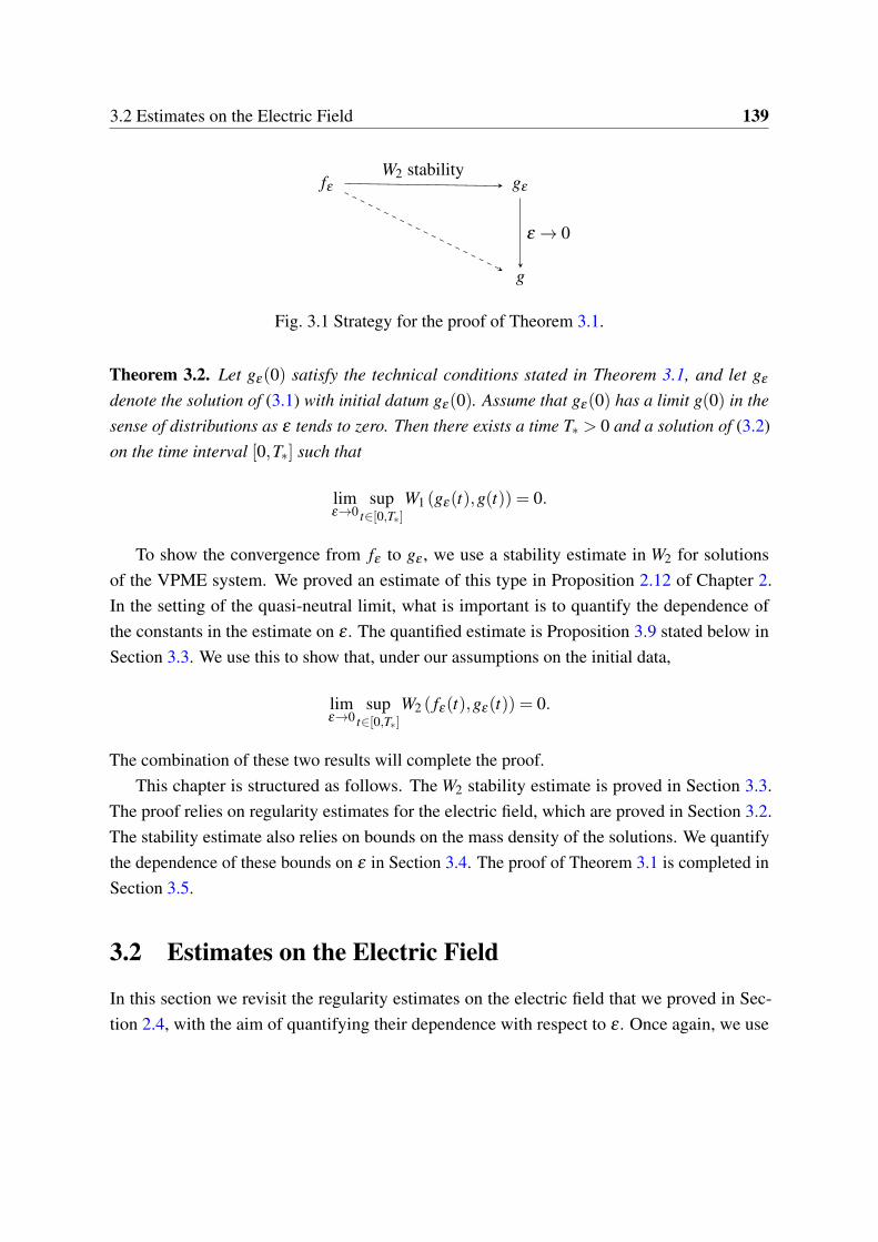
3.2 Estimates on the Electric Field 139
fε gε
g
W2 stability
ε → 0
Fig. 3.1 Strategy for the proof of Theorem 3.1.
Theorem 3.2. Let gε(0) satisfy the technical conditions stated in Theorem 3.1, and let gε
denote the solution of (3.1) with initial datum gε(0). Assume that gε(0) has a limit g(0) in thesense of distributions as ε tends to zero. Then there exists a time T∗ > 0 and a solution of (3.2)on the time interval [0,T∗] such that
limε→0
supt∈[0,T∗]
W1 (gε(t),g(t)) = 0.
To show the convergence from fε to gε , we use a stability estimate in W2 for solutionsof the VPME system. We proved an estimate of this type in Proposition 2.12 of Chapter 2.In the setting of the quasi-neutral limit, what is important is to quantify the dependence ofthe constants in the estimate on ε . The quantified estimate is Proposition 3.9 stated below inSection 3.3. We use this to show that, under our assumptions on the initial data,
limε→0
supt∈[0,T∗]
W2 ( fε(t),gε(t)) = 0.
The combination of these two results will complete the proof.This chapter is structured as follows. The W2 stability estimate is proved in Section 3.3.
The proof relies on regularity estimates for the electric field, which are proved in Section 3.2.The stability estimate also relies on bounds on the mass density of the solutions. We quantifythe dependence of these bounds on ε in Section 3.4. The proof of Theorem 3.1 is completed inSection 3.5.
3.2 Estimates on the Electric Field
In this section we revisit the regularity estimates on the electric field that we proved in Sec-tion 2.4, with the aim of quantifying their dependence with respect to ε . Once again, we use
140 The Quasi-Neutral Limit for the VPME System With Rough Data
the decomposition of the electrostatic potential into two parts:
Uε = Uε +Uε ,
where Uε and Uε are solutions of the equations
ε2∆Uε = 1−ρ[ fε ], ε
2∆Uε = eUε+Uε −1.
We will use the notation Eε =−∇Uε and Eε =−∇Uε .
3.2.1 Regularity
The following is a version of Proposition 2.4 with quasi-neutral scaling. We will give the proofof these estimates below.
Proposition 3.3 (Regularity estimates on Uε and Uε ). Let d = 2,3. Let h ∈ L∞ ∩Ld+2
d (Td).Then there exist unique Uε ∈W 1,2(Td) with zero mean and Uε ∈W 1,2 ∩L∞(Td) satisfying
ε2∆Uε = 1−h, ε
2∆Uε = eUε+Uε −1.
Moreover we have the following estimates for some constant Cα,d > 0:
∥Uε∥C0,α (Td) ≤Cα,d ε−2(
1+∥h∥L
d+2d (Td)
), α ∈
(0,1) if d = 2
(0, 15 ] if d = 3
∥Uε∥C1,α (Td) ≤Cα,d ε−2(
1+∥h∥L∞(Td)
), α ∈ (0,1)
∥Uε∥C1,α (Td) ≤Cα,d exp(
Cα,dε−2(
1+∥h∥L
d+2d (Td)
))α ∈ (0,1)
∥Uε∥C2,α (Td) ≤Cα,d exp2
(Cα,dε
−2(
1+∥h∥L
d+2d (Td)
))α ∈
(0,1) if d = 2
(0, 15 ] if d = 3.
3.2.1.1 Regularity of Uε
For the singular part of the potential Uε , the dependence on ε can be deduced using the factthat the Poisson equation is linear, that is, that
∆(ε
2Uε
)= 1−h.
By applying Lemma 2.5 from Chapter 2 to ε2Uε , we deduce the following estimates:
3.2 Estimates on the Electric Field 141
(i) If h ∈ Ld+2
d (Td), then for all α ∈ (0,1), if d = 2, or α ∈ (0, 15 ] if d = 3, there exists a
constant Cα,d > 0 such that
∥Uε∥C0,α ≤Cα,dε−2(
1+∥h∥L
d+2d (Td)
)
(ii) If h ∈ L∞(Td), then for any α ∈ (0,1), there exists a constant Cα,d such that
∥Uε∥C1,α (Td) ≤Cα,d ε−2(
1+∥h∥L∞(Td)
)We can also deduce the following quantified version of Lemma 2.6.
Lemma 3.4 (Log-Lipschitz regularity of Eε ). Let Uε be a solution of
ε2∆Uε = h
for h ∈ L∞(Td). Then
|∇Uε(x)−∇Uε(y)| ≤ ε−2C∥h∥L∞ |x− y|
(1+ log
( √d
|x− y|
)1|x−y|≤
√d
).
3.2.1.2 Regularity of Uε
In Section 2.4.2, we proved the existence of a unique W 1,2(Td) solution U of the equation
∆U = eU+U −1,
under the assumption that U ∈ L∞(Td)∩W 1,2(Td). We showed that this solution in fact belongsto the Hölder space C1,α(Td) for α ∈ (0,1). Furthermore, if U ∈C0,α(Td), then U ∈C2,α(Td).The method of proof also applies for general ε . We will revisit part of the proof here in order toquantify how the constants depend on ε .
Lemma 3.5. Consider the nonlinear Poisson equation
ε2∆Uε = eUε+Uε −1. (3.5)
Assume that Uε ∈ L∞(Td)∩W 1,2(Td) with
∥Uε∥L∞(Td) ≤ M1. (3.6)
142 The Quasi-Neutral Limit for the VPME System With Rough Data
Then the unique W 1,2(Td) solution Uε of (3.5) belongs to C1,α(Td) for all α ∈ (0,1), with theestimate
∥Uε∥C1,α (Td) ≤Cε−2 (e2M1 +1
).
If, in addition, Uε is Hölder regular with the estimate
∥Uε∥C0,α (Td) ≤ M2
for some α ∈ (0,1), then Uε ∈C2,α(Td) with the estimate
∥Uε∥C1,α (Td) ≤[M2 +Cε
−2 (e2M1 +1)]
exp[Cε
−2 (e2M1 +1)].
Proof. The idea is to prove Lp(Td) estimates on the right hand side of (3.5), in particular oneUε . The estimates on Uε are then deduced using standard regularity estimates for the Poissonequation.
Since Uε is already controlled in L∞ by assumption (3.6), it is enough to estimate eUε . Weprove an a priori estimate using the equation satisfied by Uε :
ε2∆Uε = eUε+Uε −1.
We use the function e(p−1)Uε as a test function in the weak form of this equation. Then∫Td
e(p−1)Uε dx = ε2(p−1)
∫Td
|∇Uε |2eUε dx+∫Td
eUε · epUε dx,
and so ∫Td
eUε · epUε dx ≤∫Td
e(p−1)Uε dx,
We can make this estimate rigorous by using a truncation argument, as described in the proofof Lemma 2.9. Since
∥Uε∥L∞(Td) ≤ M1,
we have∥eUε∥p
Lp(Td)≤ eM1∥eUε∥p−1
Lp−1(Td). (3.7)
Note that the constants in this estimate do not depend on ε . We therefore deduce an estimatefor all p < ∞ by induction, in the same way as we did in Lemma 2.9.
First, since0 = ε
2∫Td
∆Uε dx =∫Td
(eUε −1
)dx,
3.2 Estimates on the Electric Field 143
for any ε we still have∥eUε∥L1(Td) = 1.
Then∥eUε∥L1(Td) ≤ e∥Uε∥L∞(Td ) ≤ eM1 .
By induction, using (3.7), we conclude that for all integer p,
∥eUε∥Lp(Td) ≤ eM1. (3.8)
By interpolation, this extends to any p < ∞.Next, we use these estimates to deduce regularity for Uε . By Calderón-Zygmund estimates
for the Poisson equation,
∥Uε∥W 2,n(Td) ≤Cn,dε−2∥eUε+Uε∥Ln(Td) ≤Cn,dε
−2 (e2M1 +1).
By Sobolev embedding with n sufficiently large, for any α ∈ (0,1),
∥Uε∥C1,α (Td) ≤Cα,dε−2 (e2M1 +1
).
Now assume that for some α ∈ (0,1),
∥Uε∥C0,α (Td) ≤ M2.
Then Uε ∈C0,α(Td), with
∥Uε∥C0,α (Td) ≤ ∥Uε∥C0,α (Td)+∥Uε∥C0,α (Td) ≤ M2 +Cε−2 (e2M1 +1
).
Since ∣∣∣eUε (x)− eUε (y)∣∣∣≤ emaxUε (x),Uε (y) |Uε(x)−Uε(y)| ,
it follows that
∥eUε∥C0,α (Td) ≤ ∥Uε∥C0,α (Td) exp[Cε
−2 (1+ e2M1)].
By Schauder estimates [30, Chapter 4],
∥Uε∥C2,α (Td) ≤C(∥Uε∥L∞(Td)+ ε
−2∥eUε −1∥C0,α (Td)
)≤[M2 +Cε
−2 (1+ e2M1)]
exp[Cε
−2 (1+ e2M1)],
144 The Quasi-Neutral Limit for the VPME System With Rough Data
as required.
3.2.2 Stability
We are also interested in the stability of Uε with respect to the charge density. The propositionbelow is a quantitative version of Proposition 2.11.
Proposition 3.6. For each i = 1,2, let U (i)ε be a zero-mean solution of
ε2∆U (i)
ε = hi −1,
where hi ∈ L∞ ∩Ld+2
d (Td). Then
∥∇U (1)ε −∇U (2)
ε ∥2L2(Td) ≤ ε
−4 maxi
∥hi∥L∞(Td)W22 (h1,h2). (3.9)
Now, in addition, let U (i)ε be a solution of
ε2∆U (i)
ε = eU (i)ε +U (i)
ε −1.
Then
∥∇U (1)ε −∇U (2)
ε ∥2L2(Td) ≤ exp2
[Cdε
−2(
1+maxi
∥hi∥L(d+2)/d(Td)
)](3.10)
×maxi
∥hi∥L∞(Td)W22 (h1,h2).
For the stability of ∇Uε , we use a result proved originally by Loeper [65] in the wholespace Rd , and adapted to the torus Td in [43].
Lemma 3.7 (Loeper-type estimate for Poisson’s equation). For each i = 1,2, let U (i)ε be a
solution of
ε2∆U (i)
ε = hi −1,
where hi ∈ L∞(Td). Then
∥∇U (1)ε −∇U (2)
ε ∥2L2(Td) ≤ ε
−4 maxi
∥hi∥L∞(Td)W22 (h1,h2).
For Uε we use a version of Proposition 2.11 in which we quantify the dependence of theconstants on ε .

3.2 Estimates on the Electric Field 145
Lemma 3.8. For each i = 1,2, let U (i)ε ∈W 1,2 ∩L∞(Td) be a solution of
ε2∆U (i)
ε = eU (i)ε +U (i)
ε −1, (3.11)
for some given potentials U (i)ε ∈ L∞(Td) . Then
ε2∥∇U (1)
ε −∇U (2)ε ∥2
L2(Td) ≤Cε∥U (1)ε −U (2)
ε ∥2L2(Td),
where C depends on the L∞ norms of U (i)ε and U (i)
ε . More precisely, Cε can be chosen such that
Cε ≤ exp[C(
maxi
∥U (i)ε ∥L∞(Td)+max
i∥U (i)
ε ∥L∞(Td)
)],
for some sufficiently large constant C, independent of ε .
Proof. We look at the equation solved by the difference U (1)ε −U (2)
ε . By subtracting the twoequations (3.11), we find that
ε2∆(U (1)
ε −U (2)ε ) = eU (1)
ε +U (1)ε − eU (2)
ε +U (2)ε .
By taking U (1)ε −U (2)
ε as a test function, we find that
−ε2∫Td|∇U (1)
ε −∇U (2)ε |2 dx =
∫Td
(eU (1)
ε +U (1)ε − eU (2)
ε +U (2)ε
)(U (1)
ε −U (2)ε )dx.
In the proof of Proposition 2.11, we showed that for any U ,U ,V ,V ∈ L∞(Td),
−∫Td
(eU+U − eV+V
)(U −V )dx ≤CU,V∥U −V∥2
L2(Td),
whereCU,V ≤ exp
C[∥U∥L∞(Td)+∥U∥L∞(Td)+∥V∥L∞(Td)+∥V∥L∞(Td)
].
Thus∥∇U (1)
ε −∇U (2)ε ∥2
L2(Td) ≤Cε ε−2∥U (1)
ε −U (2)ε ∥2
L2(Td),
where
Cε ≤ exp[C(
maxi
∥U (i)ε ∥L∞(Td)+max
i∥U (i)
ε ∥L∞(Td)
)].
146 The Quasi-Neutral Limit for the VPME System With Rough Data
Proof of Proposition 3.6. It suffices to prove (3.10), since (3.9) follows immediately fromLemma 3.7. By the Poincaré inequality for zero-mean functions,
∥U (1)ε −U (2)
ε ∥2L2(Td) ≤C∥∇U (1)
ε −∇U (2)ε ∥2
L2(Td).
By Lemma 3.7,
∥∇U (1)ε −∇U (2)
ε ∥2L2(Td) ≤ ε
−4 maxi
∥hi∥L∞(Td)W22 (h1,h2).
Then, by Lemma 3.8,
∥∇U (1)ε −∇U (2)
ε ∥2L2(Td) ≤Cε ε
−6 maxi
∥hi∥L∞(Td)W22 (h1,h2),
for
Cε ≤ exp[C(
maxi
∥U (i)ε ∥L∞(Td)+max
i∥U (i)
ε ∥L∞(Td)
)].
For the L∞(Td) estimates, we use Proposition 3.3:
∥U (i)ε ∥L∞(Td) ≤Cd ε
−2(
1+∥hi∥L
d+2d
)∥U (i)
ε ∥L∞(Td) ≤Cd exp[Cdε
−2(
1+∥hi∥L
d+2d
)].
Hence
Cε ≤ exp2
[Cdε
−2(
1+maxi
∥hi∥L
d+2d
)],
which implies (3.10).
3.3 Wasserstein Stability
To prove the quasi-neutral limit, we will need a quantified stability estimate between solu-tions of the VPME system (3.1). The following proposition is an ε-dependent version ofProposition 2.12. We revisit the proof here, keeping track of how all the constants depend on ε .
Proposition 3.9 (Stability for solutions with bounded density). For i = 1,2, let f (i)ε be solutionsof (3.1) satisfying for some constant M and all t ∈ [0,T ],
ρ[ f (i)ε (t)]≤ M.

3.3 Wasserstein Stability 147
Then there exists a constant Cε such that, for all t ∈ [0,T ],
W2
(f (1)ε (t), f (2)ε (t)
)≤ β
(t,W2
(f (1)ε (0), f (2)ε (0)
)),
where β denotes the function
β (t,x) =
16deexp[(
1+ log x16d
)e−Cε t] t ≤ T0
(d ∨ x)eCε (1+log16)(t−T0) t > T0,
whereT0 = inf
t > 0 : 16deexp
[(1+ log
x16d
)e−Cε t
]> d.
If in addition, for some constant C0,
supt∈[0,T ]
∥ f (i)ε (t, ·, ·)∥L∞x,v ≤C0, sup
t∈[0,T ]E ME
ε [ f (i)ε ](t)≤C0, (3.12)
then Cε may be chosen to satisfy
Cε ≤ exp2(Cε−2)(M+1).
Proof. The W2 distance is defined as an infimum over couplings (Definition 4). Thus it sufficesto estimate the L2 distance corresponding to a particular coupling of f (1)ε and f (2)ε . To do thiswe will first represent f (i)ε as the pushforward of f (i)ε (0) along the characteristic flow inducedby f (i)ε . That is, consider the following system of ODEs for Z(i)
z =(
X (i)z ,V (i)
z
)∈ Td ×Rd:
X (i)
z =V (i)z ,
V (i)z = E(i)
ε
(X (i)
z),(
X (i)z (0),V (i)
z (0))= (x,v) = z,
(3.13)
where the electric field E(i)ε is given by
E(i)ε =−∇U (i)
ε ,
ε2∆U (i)
ε = eU (i)ε −ρ
(i)ε := eU (i)
ε −ρ[ f (i)ε ].
Since f (i)ε has bounded mass density, Proposition 3.3 and Lemma 3.4 imply that E(i)ε is a
log-Lipschitz vector field, with a constant uniform on [0,T ]. This regularity is enough toimply that there exists a unique solution of (3.13) for every initial condition z, resulting in a
148 The Quasi-Neutral Limit for the VPME System With Rough Data
well-defined characteristic flow. Since the characteristic flow is unique, by [1, Theorem 3.1]the linear Vlasov equation
∂tg+ v ·∇xg+E(i)ε (x) ·∇vg = 0,
g|t=0 = f (i)ε (0)≥ 0(3.14)
has a unique solution. Moreover, this solution can be represented, in weak form, by the relation∫Td×Rd
φ gt(dz) =∫Td×Rd
φ
(Z(i)
z
)f (i)ε (0)(dz), (3.15)
for all φ ∈Cb(Td ×Rd). Since f (i)ε is certainly a solution of (3.14), we deduce that g = f (i)ε
and so f (i)ε has the representation (3.15). We will use this representation to define a couplingbetween f (1)ε and f (2)ε .
Fix an arbitrary initial coupling π0 ∈ Π
[f (1)ε (0), f (2)ε (0)
]. We define πt to follow the
corresponding characteristic flows: for φ ∈Cb((Td ×Rd)2), let∫(Td×Rd)2
φ(z1,z2)dπt(z1,z2) =∫Td×Rd
φ
(Z(1)
z ,Z(2)z
)dπ0(z1,z2).
We can verify that πt is indeed a coupling of f (1)ε and f (2)ε by checking the marginals:∫(Td×Rd)2
φ(zi)dπt(z1,z2) =∫(Td×Rd)2
φ
(Z(i)
zi (t))
dπ0(z1,z2) (3.16)
=∫Td×Rd
φ
(Z(i)
z (t))
f (i)ε (0)(dz)
=∫Td×Rd
φ(z) f (i)ε (t)(dz).
Next, we define a functional which is greater than (or equal to) the squared Wassersteindistance between f (1)ε and f (2)ε . Let
D(t) =∫(Td×Rd)2
|x1 − x2|2 + |v1 − v2|2 dπt(z1,z2).
Since the Wasserstein distance is an infimum over couplings, while πt is a particular coupling,D must control the squared Wasserstein distance:
W 22 ( f (1)ε , f (2)ε )≤ D.
3.3 Wasserstein Stability 149
To prove our stability estimate, it therefore suffices to estimate D. We will do this using aGrönwall estimate. Taking a time derivative, we find
D = 2∫(Td×Rd)2
(X (1)
z1 (t)−X (2)z2 (t)
)·(
V (1)z1 (t)−V (2)
z2 (t))
+(
V (1)z1 (t)−V (2)
z2 (t))·(
E(1)ε (t,X (1)
z1 (t))−E(2)ε (t,X (2)
z2 (t)))
dπ0(z1,z2).
Using the Cauchy-Schwarz inequality, we obtain
D ≤ D+√
D(∫
(Td×Rd)2
∣∣∣E(1)ε (t,X (1)
z1 (t))−E(2)ε (t,X (2)
z2 (t))∣∣∣2 dπ0(z1,z2)
)1/2
.
In other words,
D ≤ D+√
D(∫
(Td×Rd)2
∣∣∣E(1)ε (t,x1)−E(2)
ε (t,x2)∣∣∣2 dπt(z1,z2)
)1/2
.
We split the electric field term into the form
∫(Td×Rd)2
∣∣∣E(1)ε (t,x1)−E(2)
ε (t,x2)∣∣∣2 dπt(z1,z2)≤C
4
∑i=1
Ii,
where
I1 :=∫(Td×Rd)2
|E(1)ε (t,x1)− E(1)
ε (t,x2)|2 dπt , I2 :=∫(Td×Rd)2
|E(1)ε (t,x2)− E(2)
ε (t,x2)|2 dπt ,
I3 :=∫(Td×Rd)2
|E(1)ε (t,x1)− E(1)
ε (t,x2)|2 dπt , I4 :=∫(Td×Rd)2
|E(1)ε (t,x2)− E(2)
ε (t,x2)|2 dπt .
Control of I1: To estimate I1, observe that by Lemma 3.4,
I1 ≤Cε−4∥ρ
(1)ε ∥2
L∞(Td)
∫(Td×Rd)2
|x1 − x2|2(
1+ log
( √d
|x1 − x2|
)1|x1−x2|≤
√d
)2
dπt .
As in Lemma 2.15, we use the function
H(x) :=
x(log x
16d
)2 if x ≤ d
d (log16)2 if x > d,

150 The Quasi-Neutral Limit for the VPME System With Rough Data
which is concave on R+. Then
I1 ≤Cε−4∥ρ
(1)ε ∥2
L∞(Td)
∫(Td×Rd)2
H(|x1 − x2|2
)dπt .
By Jensen’s inequality,
I1 ≤Cε−4∥ρ
(1)ε ∥2
L∞(Td)H(∫
(Td×Rd)2|x1 − x2|2 dπt
)≤Cε
−4M2H(D).
Control of I2: For I2, observe that
I2 ≤∫Td
|E(1)ε (x)− E(2)
ε (x)|2ρ(2)ε (dx)
≤ ∥ρ(2)ε ∥L∞(Td)∥E(1)
ε − E(2)ε ∥2
L2(Td).
We apply the Loeper stability estimate (Lemma 3.7) to obtain
I2 ≤ ε−4 max
i∥ρ
(i)ε ∥2
L∞(Td)W22 (ρ
(1)ε ,ρ
(2)ε )≤Cε
−4M2D.
Control of I3: To estimate I3, we recall a regularity estimate on U (1)ε from Proposition 3.3:
∥E(1)ε ∥C1(Td) ≤ ∥U (1)
ε ∥C2(Td) ≤Cd exp2
(Cdε
−2(
1+∥ρ(1)ε ∥
Ld+2
d (Td)
)).
Under conditon (3.12), by Lemma 1.12,
∥ρ(1)ε ∥
Ld+2
d (Td)≤C
for some C depending on C0 only. Therefore
I3 ≤ ∥E(1)ε ∥2
C1(Td)
∫(Td×Rd)2
|x1 − x2|2 dπt ≤ exp2(Cε−2)D,
for some C depending on C0 and d only. If (3.12) does not hold, we can use the fact that
∥ρ(1)ε ∥
Ld+2
d (Td)≤ ∥ρ
(1)ε ∥L∞(Td) ≤ M
and complete the proof in the same way, to find a constant depending on M.

3.3 Wasserstein Stability 151
Control of I4: First, note that
I4 =∫Td
|E(1)ε (x)− E(2)
ε (x)|2ρ(2)ε (dx)≤ ∥ρ
(2)ε ∥L∞(Td)∥E(1)
ε − E(2)ε ∥2
L2(Td).
We apply the stability estimate on U (1)ε from Proposition 3.6 to find
∥E(1)ε − E(2)
ε ∥2L2(Td) ≤ exp2
[Cdε
−2(
1+maxi
∥ρ(i)ε ∥L(d+2)/d(Td)
)]×max
i∥ρ
(i)ε ∥L∞(Td)W
22 (ρ
(1)ε ,ρ
(2)ε ).
Once again, if conditon (3.12) holds then
∥E(1)ε − E(2)
ε ∥2L2(Td) ≤ exp2
(Cε
−2)maxi
∥ρ(i)ε ∥L∞(Td)W
22 (ρ
(1)ε ,ρ
(2)ε ),
for some C depending on C0 and d only. Thus
I4 ≤ exp2(Cε
−2)M2D.
Altogether we find that
D ≤
CεD(1+ |log D
16d |)
if D < d
Cε(1+ log16)D if D ≥ d.
If (3.12) holds, then Cε may be chosen to satisfy
Cε ≤Cε−2M+ exp2(Cε
−2)+ exp2(Cε−2)M
≤ exp2(Cε−2)(M+1).
We conclude thatD(t)≤ β (t,D(0)) ,
following the argument used in the proof of Lemma 2.14.

152 The Quasi-Neutral Limit for the VPME System With Rough Data
3.4 Growth Estimates
In this section we will study how the support of a solution of the VPME system grows in time.We present two different proofs for the two and three dimensional case, respectively in Sections3.4.1 and 3.4.2. The result we obtain is the following:
Proposition 3.10 (Mass bounds). Let fε be a solution of (3.1) satisfying for some constant C0,
∥ fε∥L∞([0,T ]×Td×Rd) ≤C0, supt∈[0,T ]
E MEε [ fε(t)]≤C0.
Assume that ρ fε ∈ L∞([0,T ];L∞(Td)). Let R0 be any constant such that the support of fε(0, ·, ·)is contained in Td ×BRd(0,R0).
(i) If d = 2, then:sup
t∈[0,T ]∥ρ fε (t)∥L∞(T2) ≤CT eCε−2 [
R0 + ε−2]2 .
The constant C depends on C0 only, while CT depends on C0 and T .
(ii) If d = 3, then:
supt∈[0,T ]
∥ρε(t)∥L∞(T3) ≤ maxT−81/8,C(R30 + eCε−2
T 6).
The constant C depends on C0 only.
3.4.1 Proof of Proposition 3.10 in the two dimensional case
In this section, we prove an estimate on the mass density ρε in the case d = 2. Observe firstthat if the support of fε is contained in the set T2 ×BR2(0;Rt), then
∥ρε(t)∥L∞(Td) ≤CR2t , (3.17)
where C is a constant depending on ∥ fε(0)∥L∞(T2×R2). Our argument will rely on controllingthe growth of the support of fε . To do this we will find a bound on the growth rate of thevelocity component of the characteristic trajectories. Since any characteristic trajectory (Xt ,Vt)
satisfiesVt = Eε(Xt),
we look for a uniform estimate on the electric field Eε .

3.4 Growth Estimates 153
By Proposition 3.3, for the smooth part Eε we have the estimate
∥Eε∥L∞(T2) ≤ exp
Cε−2(
1+∥ρε∥L2(T2)
)≤ exp
(Cε
−2),where the constant C depends only on a bound on the initial energy. However, for the singularpart Eε , Proposition 3.3 only gives us the estimate
∥Eε∥L∞(T2) ≤Cε−2(
1+∥ρε∥L∞(Td)
),
which depends on an L∞ bound on the mass density. If we use this estimate in combinationwith (3.17), this results in a bound on the size of the support of the form
Rt ≤ R0 + exp(Cε
−2)t +Cε−2∫ t
0R2
s ds. (3.18)
The solution of the ODEy =C(1+ y2)
blows up in finite time and so the differential inequality (3.18) is not enough to imply a boundon Rt . We need to use a more careful estimate on Eε . In dimension two, we can make use of thefact that the conservation of energy gives us a uniform bound on ∥ρε∥L2(T2), by Lemma 1.12,and use an interpolation argument.
Lemma 3.11. Let ρ ∈ L1 ∩L∞(T2) satisfy the bounds
∥ρ∥L1(T2) = 1, ∥ρ∥L2(T2) ≤C0, ∥ρ∥L∞(T2) ≤ M.
Let Eε =−∇Uε , where Uε is the unique W 1,2(T2) solution of the Poisson equation
ε2∆Uε = 1−ρ.
Then there exists a constant C depending only on C0 such that
∥Eε∥L∞(T2) ≤Cε−2(
1+ | logM|1/2).
Proof. We use the representation
Eε = ε−2Kper ∗ (ρ −1) =Cε
−2∫[− 1
2 ,12 ]
2
y|y|2
(ρ(x− y)−1)dy+ ε−2K0 ∗ (ρ −1),

154 The Quasi-Neutral Limit for the VPME System With Rough Data
where K0 is a C1(T2) function. By Young’s inequality,
∥K0 ∗ (ρ −1)∥L∞(T2) ≤ ∥K0∥L∞(T2)∥ρ −1∥L1(T2) ≤C.
We split the integral term into a part where |y| is small and a part where |y| is large:∫[− 1
2 ,12 ]
2
y|y|2
(ρ(x− y)−1)dy =∫|y|≤l
y|y|2
(ρ(x− y)−1)dy+∫
2≥|y|≥l
y|y|2
(ρ(x− y)−1)dy.
For the part where |y| is large, we use Young’s inequality with the L2 control on ρ:∣∣∣∣∫2≥|y|≥l
y|y|2
(ρ(x− y)−1)dy∣∣∣∣≤ ∫2≥|y|≥l
1|y|
|ρ(x− y)−1|dy
≤∥∥∥∥ 1|y|12≥|y|≥l ∗ |ρ −1|
∥∥∥∥L∞(T2)
≤(∫
2≥|y|≥l
1|y|2
dy)1/2
∥ρ −1∥L2(T2)
≤C(C0 +1) | log l|1/2.
Where |y| is small, we use Young’s inequality with the L∞ control on ρ:∣∣∣∣∫|y|≤l
y|y|2
(ρ(x− y)−1)dy∣∣∣∣≤ ∫|y|≤l
1|y|
|ρ(x− y)−1|dy
≤∥∥∥∥ 1|y|1|y|≤l ∗ |ρ −1|
∥∥∥∥L∞(T2)
≤ ∥ρ −1∥L∞(T2)
∫|y|≤l
1|y|
dy
≤CM l.
Altogether we obtain
∥Eε∥L∞(T2) ≤Cε−2[1+C0| log l|1/2 +Ml
].
We choose l = M−1 and conclude that
∥Eε∥L∞(T2) ≤Cε−2(
1+ | logM|1/2),
where C depends on C0 only.

3.4 Growth Estimates 155
By using this estimate, we can deduce a differential inequality on Rt that can be closed.
Lemma 3.12. Let fε be a solution of (3.1) with bounded energy and compact support containedin T2 ×BR2(0;Rt) at time t. Then R satisfies the estimate
Rt ≤ eCε−2t (1+R0 +(log t ∨0)) .
Proof. We consider the velocity coordinate Vt(x,v) of an arbitrary characteristic trajectorystarting from (x,v) at time t = 0. We have
|Vt(x,v)| ≤ |v|+∫ t
0∥Eε∥L∞(T2) ds
≤ |v|+∫ t
0∥Eε∥L∞(T2)+∥Eε∥L∞(T2) ds
≤ |v|+∫ t
0exp(Cε
−2)+Cε−2(
1+ | logRs|1/2)
ds
The size of the support is controlled by the modulus of the furthest-reaching characteristictrajectory that starts within the support of fε(0):
Rt ≤ sup(x,v)∈T2×BR2(0;R0)
|Vt(x,v)|
≤ sup(x,v)∈T2×BR2(0;R0)
|v|+
∫ t
0exp(Cε
−2)+Cε−2(
1+ | logRs|1/2)
ds
≤ R0 +∫ t
0exp(Cε
−2)+Cε−2| logRs|1/2 ds.
We compare this with the function
z(t) = (1+2Ct) [R0 + log(1+2Ct)] .
By Lemma A.1, this satisfiesz ≥C(1+ log(1+ z)).
We deduce thatRt ≤ eCε−2
t(ε−2 +R0 +(log t ∨0)
).
156 The Quasi-Neutral Limit for the VPME System With Rough Data
Proof of Proposition 3.10, case d = 2. We combine Lemma 3.12 with the elementary estimate(3.17): for all t ∈ [0,T ],
∥ρε(t)∥L∞(Td) ≤CR2t
≤ eCε−2t(ε−2 +R0 +(log t ∨0)
)2
≤CT eCε−2 (R0 + ε
−2)2.
3.4.2 Proof of Proposition 3.10 in the three dimensional case
In this section, we prove a mass bound in the case d = 3. In this case, the conservation ofenergy gives us a uniform bound on ∥ρε∥L5/3(T3). This integrability is not enough to allow usto use the elementary interpolation approach that we used in the the two dimensional case.Instead, we will adapt estimates devised by Batt and Rein [10] for the classical Vlasov-Poissonequation on T3 ×R3. We used this approach in Chapter 2 to prove the existence of solutionsof the VPME system with bounded density. Here we focus on identifying how the bounds on∥ρε∥L∞(T3) depend on ε .
As in the two dimensional case, Batt and Rein’s argument relies on controlling the massdensity using the characteristic trajectory with velocity component of greatest Euclidean normstarting within the support of fε(0) at time zero. They prove a bootstrap estimate on theconvolution integral defining the singular part of the electric field. We recall this estimate in thefollowing technical lemma.
Lemma 3.13. Let (X(t;s,x,v),V (t;s,x,v)) denote the solution at time t of an ODE(X(t)V (t)
)= a(t,X(t),V (t)),
(X(s)V (s)
)=
(xv
),
where a is of the form
a(t,X ,V ) =
(V
a2(t,X ,V )
),
for some vector-field a2 : [0,T ]×T3 ×R3 → R3.Assume that, for t ∈ [0,T ], f = f (t,x,v) is the pushforward of f0 along the associated
characteristic flow; that is, for all φ ∈Cb(T3 ×R3),∫T3×R3
f (t,x,v)φ(x,v)dxdv =∫T3×R3
f (s,x,v)φ(X(t;s,x,v),V (t;s,x,v))dxdv.
3.4 Growth Estimates 157
Assume that there exists C∗ > 1 such that
∥ f∥L∞([0,T ]×T3×R3) ≤C∗, supt∈[0,T ]
∥ ft |v|2∥L1(T3×R3) ≤C∗.
Also, suppose that, for some β ∈ (0,1),
hη(t,∆)≤C∗hρ(t)β∆ for all hρ(t)−β ≤ ∆ ≤ t, (3.19)
where hρ ,hη are defined as in (2.47). Then for all 0 ≤ t1 < t2 ≤ t with t2 − t1 ≤ ∆, if
hρ(t)−β/2 ≤ ∆ ≤ t
then ∫ t2
t1
∫T3|X(s)− y|−2
ρ f (s,y)dyds ≤C(
hρ(t)2β/3 +hρ(t)1/6)
∆,
where C depends only on C∗.
We complete the proof of Proposition 3.10 by combining Lemma 3.13 with the estimateson Eε from Proposition 3.3.
Proof of Proposition 3.10, case d = 3. For any characteristic trajectory (Xt ,Vt), we have forany 0 ≤ t1 < t2 ≤ T ,
|Vt1 −Vt2| ≤∫ t1
t2|Eε(Xs)|ds.
We can write the total force Eε in the form
Eε(x) = ε−2[K0 ∗ (ρε −1)](x)+Cε
−2∫T3
x− y|x− y|3
ρε(y)dy+ Eε .
Since K0 is a C1(T3) function and ρε has unit mass, the first term satisfies the bound
|ε−2[K0 ∗ (ρε −1)](x)| ≤ ε−2∥K0∥L∞(T3)∥ρε −1∥L1(T3)
≤Cε−2.
For the last term, we use Proposition 3.3:
|Eε | ≤ exp[C(
1+∥ρε∥L5/3(T3)
)]≤ exp(Cε
−2).

158 The Quasi-Neutral Limit for the VPME System With Rough Data
Therefore,
|Vt1 −Vt2| ≤∫ t1
t2
[exp(Cε
−2)+Cε−2∫T3|X(s)− y|−2
ρε(y)dy]
ds. (3.20)
From [50, Lemma 4.5.4] we have the estimate∫T3|x− y|−2
ρε(s,y)dy ≤C∥ρε(s, ·)∥5/9L5/3∥ρε(s, ·)∥4/9
L∞(T3)≤C∥ρε(s, ·)∥4/9
L∞(T3),
where C depends only on ∥ fε(0)∥L∞(T3×R3) and the initial energy.By (3.20), we have
hη(t,∆)≤(
Cε−2hρ(t)
49 + eCε−2
)∆.
Since ρε has total mass 1, hρ ≥ 1. Thus
hη(t,∆)≤ eCε−2∆hρ(t)
49 .
This means that condition (3.19) is satisfied with C∗ = eCε−2. We apply Lemma 3.13 to improve
our bound on ∫T3|X(s)− y|−2
ρε(y)dy ≤CC4/3∗(
hρ(t)23 ·
49 +hρ(t)1/6
)∆.
Feeding this new estimate into (3.20), we obtain
hη(t,∆)≤Cε−2C4/3
∗(
hρ(t)23 ·
49 +hρ(t)1/6
)∆+(Cε
−2 +CeCε−2)∆ ≤ eCε−2
hρ(t)8
27 ∆,
as long ashρ(t)−2/9 ≤ ∆ ≤ t.
We will iterate this process until we achieve the lowest possible exponent for hρ , i.e. 16 .
Applying Lemma 3.13 a second time, we obtain∫T3|X(s)− y|−2
ρε(y)dy ≤CC4/3∗(
hρ(t)23 ·
827 +hρ(t)1/6
)∆,
with C∗ = eCε−2, provided that
hρ(t)−4/27 ≤ ∆ ≤ t,

3.4 Growth Estimates 159
and therefore
hη(t,∆)≤Cε−2C4/3
∗(
hρ(t)23 ·
827 +hρ(t)1/6
)∆+(Cε
−2 +CeCε−2)∆ ≤ eCε−2
hρ(t)1681 ∆.
Applying Lemma 3.13 once more, we obtain∫T3|X(s)− y|−2
ρε(y)dy ≤CC4/3∗(
hρ(t)23 ·
1681 +hρ(t)1/6
)∆,
with C∗ = eCε−2, provided that
hρ(t)−8/81 ≤ ∆ ≤ t,
and therefore
hη(t,∆)≤Cε−2C4/3
∗(
hρ(t)23 ·
1681 +hρ(t)1/6
)∆+(Cε
−2 +CeCε−2)∆ ≤ eCε−2
hρ(t)16 ∆, (3.21)
since 32243 < 1
6 and hρ ≥ 1.Finally, we use this new growth estimate on characteristic trajectories to control the mass
density. Assuming that fε(0) is supported in T3 ×BR3(0;Rt), we have
hρ ≤C∥ fε∥L∞(Td×Rd) (R0 +hη(t, t))3
Since we work with L∞(Td ×Rd) solutions, we have a uniform bound on ∥ fε∥L∞(Td×Rd)
depending only on the initial data. Therefore, using (3.21), we find that if hρ(t)−8/81 ≤ t,
hρ ≤C (R0 +hη(t, t))3 ≤C
(R0 + eCε−2
hρ(t)16 t)3
≤CR30 + eCε−2
hρ(t)1/2t3 ≤CR30 +
(eCε−2
t3)2+hρ(t)
2.
Hencehρ ≤C
(R3
0 + eCε−2t6).
If instead hρ(t)−8/81 ≥ t, thenhρ(t)≤ t−
818 .
Therefore, we may conclude that
hρ(t)≤ maxt−81/8,C(R30 + eCε−2
t6).

160 The Quasi-Neutral Limit for the VPME System With Rough Data
3.5 Quasi-Neutral Limit
In this section, we complete the proof of Theorem 3.1.
Proof of Theorem 3.1. Let gε denote the solution of (3.1) with data gε(0). We will use gε
to interpolate between the solution fε of (3.1) starting from fε(0) and the solution g of (3.2)starting from g(0). By the triangle inequality,
W1( fε(t),g(t))≤W1( fε(t),gε(t))+W1(gε(t),g(t)). (3.22)
By Theorem 3.2, there exists a solution g of (3.2) such that
limε→0
supt∈[0,T∗]
W1(gε(t),g(t)) = 0. (3.23)
To deal with the first term of (3.22), we use a stability estimate around gε for the VPMEsystem. By the monotonicity property of Wasserstein distances (1.38) and Proposition 3.9,
W1( fε(t),gε(t))≤W2( fε(t),gε(t)) (3.24)
≤
C exp[C(
1+ log W2( fε (0),gε (0))4√
d
)e−Cε t
]if W2( fε(0),gε(0))≤ d
W2( fε(0),gε(0))eCε t if W2( fε(0),gε(0))> d.
where Cε may be chosen to satisfy
Cε ≤ exp2(Cε−2)(M+1).
for any M satisfyingsup[0,T∗]
∥ρ fε (t)∥L∞x , sup
[0,T∗]∥ρgε
(t)∥L∞x ≤ M.
By Proposition 3.10, we may take M such that
M ≤C eCε−2.
The constant C depends on T∗, C0, the dimension d, and C1, the rate of growth of the initialsupport. We emphasise again that the appearance of an exponential rate here is a consequenceof the form of the equation rather than because condition (3.3) allows fast growth of the initial

3.5 Quasi-Neutral Limit 161
support. It follows that we may estimate
Cε t ≤C exp2(Cε−2)
for all t ∈ [0,T∗]. Hence we have convergence if∣∣∣log W2( fε (0),gε (0))4√
d
∣∣∣exp3(Cε−2)
→ ∞
as ε tends to zero. This holds if
W2( fε(0),gε(0))≤ (exp4(Cε−2))−1
for sufficiently large C. In this case, it follows by (3.24) that
limε→0
supt∈[0,T∗]
W1( fε(t),gε(t)) = 0.
Combined with (3.23) and (3.22), this completes the proof.

Chapter 4
Derivation of the VPME System from aSystem of Extended Ions
4.1 Introduction
In this chapter, we derive the VPME system (2.1) from a microscopic particle system. TheVPME system is a model for the ions in a plasma, assuming that the electrons are instanta-neously thermalised. A possible choice of microscopic system would therefore be a system ofN ions, modelled as point charges, in a background of thermalised electrons. On the torus, thisis described by the following system of ODEs:
Xi =Vi
Vi =1N
N
∑j =i
Kper(Xi −X j)−Kper ∗ eU ,(4.1)
where U satisfies
∆U = eU − 1N
N
∑i=1
δXi.
The formal limit of this particle system, as N tends to infinity, is the VPME system, whichreads as follows on the torus:
(V PME) :=
∂t f + v ·∇x f +E ·∇v f = 0,E =−∇xU,
∆xU = eU −∫Rd
f dv = eU −ρ,
f |t=0 = f0 ≥ 0,∫Td×Rd
f0 dxdv = 1.
(4.2)
164 Derivation of the VPME System from a System of Extended Ions
In fact, we will not be able to derive VPME from the point charge system (4.1). This isdue to the singularity of the Coulomb interaction, as discussed in Section 1.6. Instead, we willconsider a limit from a regularised system. We use a regularisation method inspired by thework of Lazarovici [61] for the classical VPME system. The idea of the proof is to use a modelconsisting of ‘extended charges’. Instead of modelling the ions as point charges, we replacethese with delocalised packets of charge. We define this system in detail in Subsection 4.1.1below.
4.1.1 The Extended Ions Model
In this section, we introduce the extended ions model. We fix a smooth, radially symmetricfunction χ : Rd → [0,+∞) with unit mass and compact support contained within the unit ballin Rd . Define
χr(x) = r−dχ
(xr
). (4.3)
We then consider a microscopic system describing the dynamics of a system of ‘delocalisedions’ of shape χr. For 1 ≤ i ≤ N, let (Xi,Vi) denote the position and velocity of the centre ofthe ith delocalised ion. The system is described by the following system of ODEs:Xi =Vi
Vi =1N ∑ j =i χr ∗Kper ∗χr(Xi −X j)−χr ∗Kper ∗ eU ,
(4.4)
where U satisfies
∆U(x) = eU(x)− 1N
N
∑i=1
χr(x−Xi)
and Kper denotes the Coulomb kernel on Td , defined in (1.44). That is, Kper =−∇Gper, whereGper = G+G0 for G0 a smooth function and G the Coulomb potential on Rd , defined by (1.42).
Note that we can rewrite the velocity equation as
Vi =−χr ∗∇U(t,Xi),
and the equation for U as∆U = eU −χr ∗ρµN
r,
4.2 Statement of Results 165
where µNr denotes the empirical measure as defined in (1.58). This is valid because χr ∗Kper ∗
χr(0) = 0, and so
1N ∑
j =iχr ∗Kper ∗χr(Xi −X j) =
1N
N
∑j=1
χr ∗Kper ∗χr(Xi −X j) = χr ∗Kper ∗χr ∗ρµNr(Xi).
Indeed, since Kper is odd and χr is even, we have
χr ∗Kper ∗χr(0) =∫Td×Td
χr(−x)Kper(x− y)χr(y)dxdy
=∫Td×Td
χr(−y)Kper(y− x)χr(x)dxdy
=−∫Td×Td
χr(y)Kper(x− y)χr(−x)dxdy
=−χr ∗Kper ∗χr(0).
4.2 Statement of Results
The main result of this chapter is the following theorem.
Theorem 4.1 (Regularised mean field limit). Let d = 2,3, and let f (0) ∈ L1 ∩L∞(Td ×Rd)
be a compactly supported choice of initial datum for (4.2). Then, for all T∗ > 0, there existsa constant C = C( f0,T∗) such that the following holds. Assume that r = rN and the initialconfigurations for (4.4) are chosen such that the corresponding empirical measures satisfy,
limsupr→0
W 22 ( f (0),µN
r (0))
rd+2+C| logr|−1/2 < 1. (4.5)
Then the empirical measure associated to the particle system dynamics starting from thisconfiguration converges to f :
limr→0
supt∈[0,T∗]
W2( f (t),µNr (t)) = 0.
Remark 5. This result in fact holds for any choice of initial data for which there exists a constantM > 0 such that for all r > 0,
∥ρ f ∥L∞([0,T∗]×Td), supr>0
∥ρ fr∥L∞([0,T∗]×Td) ≤ M.
In this case, the constant C( f0,T∗) =CM,T∗ in fact depends only on M and T∗.

166 Derivation of the VPME System from a System of Extended Ions
For Theorem 4.1 to be useful, we need to check whether the condition (4.5) is reasonable.This is dealt with in the following result. We consider data chosen randomly, by drawingindependent samples from f0. A generalised Glivenko–Cantelli theorem - a law of largenumbers result for measures - implies that µN(0) chosen in this way will converge to f0 almostsurely as N tends to infinity. With a suitable choice of parameters, the rate of this convergencewill be fast enough to satisfy (4.5).
Theorem 4.2 (Typicality). Let d = 2 or 3, and let f0 be a choice of initial datum for (4.2)satisfying the assumptions of Theorem 4.1 and having a finite kth moment for some k > 4:∫
Td×Rd
(|x|k + |v|k
)f0(dxdv)<+∞.
Let r = cN−γ for some γ satisfying
γ <1
d +2min
1d,1− 4
k
. (4.6)
For each N, select initial configurations for the regularised N-particle system (4.4) by takingN independent samples from f0. Then with probability 1, this gives an admissible set ofconfigurations for Theorem 4.1, i.e. the regularised mean field limit holds:
limN→∞
supt∈[0,T∗]
W2(µNr (t), f (t)) = 0.
Remark 6. It is worth noticing that our assumptions on r are the same as the ones found byLazarovici for the classical Vlasov–Poisson system in [61].
4.2.1 Strategy
The overall strategy is to apply the approach of Lazarovici [61] for the Vlasov–Poisson system,with appropriate modifications to adapt it to the VPME case. In this section, we briefly outlinethis approach.
The regularised mean field limit is proved in two stages. As an intermediate step betweenthe particle system (1.63) and VPME, we introduce the following regularised version of theVPME system (4.2):
∂t fr + v ·∇x fr +Er ·∇v fr = 0,Er =−χr ∗∇Ur,
∆Ur = eUr −χr ∗ρ[ fr],
fr|t=0 = f (0)≥ 0,∫Td×Rd f (0)dxdv = 1.
(4.7)
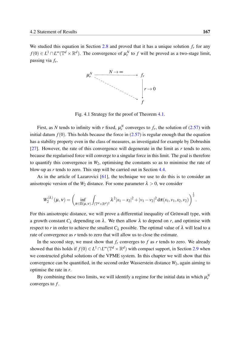
4.2 Statement of Results 167
We studied this equation in Section 2.8 and proved that it has a unique solution fr for anyf (0) ∈ L1 ∩L∞(Td ×Rd). The convergence of µN
r to f will be proved as a two-stage limit,passing via fr.
µNr fr
f
N → ∞
r → 0
Fig. 4.1 Strategy for the proof of Theorem 4.1.
First, as N tends to infinity with r fixed, µNr converges to fr, the solution of (2.57) with
initial datum f (0). This holds because the force in (2.57) is regular enough that the equationhas a stability property even in the class of measures, as investigated for example by Dobrushin[27]. However, the rate of this convergence will degenerate in the limit as r tends to zero,because the regularised force will converge to a singular force in this limit. The goal is thereforeto quantify this convergence in W2, optimising the constants so as to minimise the rate ofblow-up as r tends to zero. This step will be carried out in Section 4.4.
As in the article of Lazarovici [61], the technique we use to do this is to consider ananisotropic version of the W2 distance. For some parameter λ > 0, we consider
W (λ )2 (µ,ν) =
(inf
π∈Π(µ,ν)
∫(Td×Rd)2
λ2|x1 − x2|2 + |v1 − v2|2 dπ(x1,v1,x2,v2)
) 12
.
For this anisotropic distance, we will prove a differential inequality of Grönwall type, witha growth constant Cλ depending on λ . We then allow λ to depend on r, and optimise withrespect to r in order to achieve the smallest Cλ possible. The optimal value of λ will lead to arate of convergence as r tends to zero that will allow us to close the estimate.
In the second step, we must show that fr converges to f as r tends to zero. We alreadyshowed that this holds if f (0) ∈ L1 ∩L∞(Td ×Rd) with compact support, in Section 2.9 whenwe constructed global solutions of the VPME system. In this chapter we will show that thisconvergence can be quantified, in the second order Wasserstein distance W2, again aiming tooptimise the rate in r.
By combining these two limits, we will identify a regime for the initial data in which µNr
converges to f .

168 Derivation of the VPME System from a System of Extended Ions
The main difference in adapting the proof to the VPME case is to include the additionalpart of the electric field E =−∇U , where
∆U = eU+U −1, −∆U = ρ[ f ]−1,
and the analogous part of the electric field for the regularised equation (4.7). This is ac-complished by making use of the regularity and stability estimates on the electric field fromSections 2.4 and 2.5.
4.3 Preliminary Estimates
4.3.1 Behaviour of the Wasserstein distance under regularisation
We recall some useful results on the behaviour of Wasserstein distances under regularisation byconvolution. See [83, Proposition 7.16] for proofs. The first observation is that regularisingtwo measures cannot increase the Wasserstein distance between them.
Lemma 4.3. Let µ , ν be probability measures, r > 0 any positive constant and χr a mollifieras defined in (4.3), where χ ∈C∞
c (Rd; [0,+∞)) has total mass one. Then
Wp(χr ∗µ,χr ∗ν)≤Wp(µ,ν).
We also have an explicit control on the Wasserstein distance between a measure and itsregularisation:
Lemma 4.4. Let µ be a probability measure and r > 0. Let χr be a mollifier as defined in (4.3),where χ ∈C∞
c (Rd; [0,+∞)) has support contained in the unit ball and total mass one. Then
Wp(χr ∗µ,µ)≤ r.
If a measure ν is close to an Lp-function in Wasserstein sense, then it is possible to estimatethe Lp-norm of the regularised measure χr ∗ ν in a way that exploits this fact. We will usethis in our estimates to control the regularised mass density χr ∗ρµ . The following estimate isshown in the whole space for p = ∞ in [61, Lemma 4.3] (see also [13] for similar estimates),but it is straightforward to adapt it to the case of the torus with general p. We revisit the proofhere for completeness.
4.3 Preliminary Estimates 169
Lemma 4.5. Let ν be a probability measure on Td and h ∈ Lp(Td) a probability densityfunction, for some p ∈ [1,+∞]. Then then exists a constant Cd,χ,p, depending on the dimensiond, the integrability exponent p and ∥χ∥L∞(Td), such that for all r ∈ (0, 1
2 ], q ∈ [1,+∞),
∥χr ∗ν∥Lp(Td) ≤Cd,χ
(∥h∥Lp(Td)+r−(q+d)W q
q (h,ν)).
Proof. Throughout the proof, we identify functions and measures defined over the flat torus Td
with Zd-periodic functions and measures defined on Rd .We give the proof in the case where the Wasserstein distance Wp is defined using the toroidal
distancedTd(x,y) := inf
k∈Zd|x− y+ k|.
Note that dTd is less than or equal to the distance dQd induced by the identification of the
torus Td with the unit cube Qd =[−1
2 ,12
] 12 . The same result will therefore then also apply to
Wasserstein distances defined using dQd .Step 1: Kantorovich Duality. The proof is based on the characterisation of Wassersteindistances in terms of Kantorovich duality, which was stated in Lemma 1.6. In particular thismeans that for all pairs of functions (φ ,ψ) ∈ L1(Td,ν)×L1(Td,h) such that
φ(x)−ψ(y)≤ dTd(x,y)q
the following inequality holds:
W qq (h,ν)≥
∫Td
φ(x)ν(dx)−∫Td
ψ(y)h(y)dy.
In particular this holds if we choose ψ = φ∗, where φ∗ is the conjugate function of φ withrespect to the cost function dTd(x,y)q:
φ∗(x) := sup
y∈Tdφ(y)−dTd(x,y)q.
Now consider the mollification χr ∗ν . We make use of the identification of the torus Td
with the unit cube Qd . For a fixed x ∈ Qd , we may write
χr ∗ν(x) :=∫
x−Qd
r−dχ
(x− y
r
)ν(dy).
170 Derivation of the VPME System from a System of Extended Ions
In the expression above, the measure ν on Qd is identified with its periodic extension to Rd .The function χ is only evaluated over the principal domain Qd; note that the restriction r ≤ 1
2is imposed so that the support of χr is entirely contained within Qd . Then
χr ∗ν(x) = r−(d+q)∫
x−Qd
rqχ
(x− y
r
)ν(dy).
Define a function φx : x−Qd → R by
φx(y) := rqχ
(x− y
r
).
Note that, for r ≤ 1/2, φx = 0 on the boundary of x−Qd , and so φx can be extended periodicallyto the whole of Rd , thus inducing a well-defined function on Td .
Then we may write χr ∗ν(x) in terms of φx and its conjugate:
χr ∗ν(x) = r−(d+q)∫
x−Qd
φx(y)ν(dy)
= r−(d+q)[∫
x−Qd
φx(y)ν(dy)−∫
x−Qd
φ∗x (y)h(y)dy
]+ r−(d+q)
∫x−Qd
φ∗x (y)h(y)dy.
The conjugate function φ∗x : Td → R is defined by
φ∗x (y) := sup
z∈x−Qd
φx(z)−dTd(y,z)q.
We wish to use the bound
χr ∗ν(x)≤ r−(d+q)W qq (h,ν)+ r−(d+q)
∫x−Qd
|φ∗x (y)|h(y)dy. (4.8)
To make this rigorous, we must check that φx ∈ L1(ν) and φ∗x ∈ L1(h). For φx, we use the fact
that∥φx∥L∞ ≤ rq∥χ∥L∞ .
Thus, since ν is a finite measure, φx ∈ L1(ν). The relevant estimates on φ∗x will be proved in
Step 2 below.It then remains to to control the term
r−(d+q)∫
x−Qd
|φ∗x (y)|h(y)dy.
This is done by studying the support of φ∗x .

4.3 Preliminary Estimates 171
Step 2: Support of φ∗x . By definition,
φ∗x (y) = sup
z∈x−Qd
α(z;x,y),
where
α(z;x,y) = rqχ
(x− z
r
)−dTd(y,z)q.
First, we note some global lower and upper bounds. For the lower bound, let k ∈ Zd be suchthat y+ k ∈ x−Qd (such a k always exists), and consider the choice z = y+ k. We find that
α(y;x,y) = rqχ
(x− (y+ k)
r
)≥ 0,
since the function χ is non-negative. Thus φ∗x (y)≥ 0 for all y ∈ Td .
For the upper bound, since χ is a bounded function, we have the estimate
α(z;x,y)≤ rq ∥χ∥L∞(Td)−dTd(y,z)q ≤ rq ∥χ∥L∞(Td).
Thus∥φ
∗x ∥L∞(Td) ≤ rq ∥χ∥L∞(Td). (4.9)
Note that in particular this implies that φ∗x ∈ Lp′(Td), where p′ is the Hölder conjugate of p,
and so φ∗x belongs to L1(h). Thus the estimate (4.8) is rigorous.
Next we will control the support of φ∗x . Firstly, since the support of χ is contained in the
unit ball, if dTd(x,z)> r then
α(z;x,y) =−dTd(y,z)q ≤ 0.
Secondly, if dTd(y,z)> ηr for some η > 0, then
α(z;x,y)≤ rq[∥χ∥L∞(Td)−η
q].
If we choose η = ∥χ∥1q
L∞(Td), then
α(z;x,y)≤ 0.
It follows that, if φ∗x (y)> 0, then the intersection
BTd(x;r)∩BTd(y;∥χ∥1q
L∞(Td)r) (4.10)

172 Derivation of the VPME System from a System of Extended Ions
must be non-empty. Here BTd(z;r) denotes the ball with radius r and centre z on Td withrespect to dTd . The set (4.10) is non-empty if and only if
dTd(x,y)≤ r(
1+∥χ∥L∞(Td)
).
We deduce thatsuppφ
∗x ⊂ BTd
(x;r(
1+∥χ∥L∞(Td)
)).
Step 3: Lp estimate. Using the upper bound (4.9), it then follows that, for all y ∈ x−Qd ,
φ∗x (y)≤ rq ∥χ∥L∞(Td)1BRd (0; 1
4 )
(4(x− y)
r(1+∥χ∥L∞(Td))
),
where BRd(0;δ ) denotes the open ball in Rd of radius δ with respect to the Euclidean metric.Define the function Ψd,χ : Qd → R by
Ψd,χ(z) := rq ∥χ∥L∞(Td)1BRd (0; 14 )
(4z
r(1+∥χ∥L∞(Td))
).
This can be extended periodically to the whole of Rd and thus induces a well-defined functionon Td .
We may then write∫x−Qd
|φ cx (y)|h(y)dy =
∫x−Qd
φcx (y)h(y)dy ≤
∫x−Qd
Ψd,χ(x− y)h(y)dy = Ψd,χ ∗h(x).
Thusχr ∗ν(x)≤ r−(d+q)W q
q (h,ν)+ r−(d+q)Ψd,χ ∗h(x).
Since the torus has finite volume, we then deduce that, for all p ∈ [1,+∞],
∥χr ∗ν∥Lp(Td) ≤Cd r−(d+q)W qq (h,ν)+ r−(d+q)∥Ψd,χ ∗h∥Lp(Td).
The next step is to apply Young’s inequality to the second term:
r−(d+q)∥Ψd,χ ∗h∥Lp(Td) ≤ r−(d+q)∥Ψd,χ∥L1(Td)∥h∥Lp(Td).
4.3 Preliminary Estimates 173
The final step is to evaluate ∥Ψd,χ∥L1(Td):
∥Ψd,χ∥L1(Td) = rq ∥χ∥L∞(Td)
∫Qd
1BRd (0; 14 )
(4z
r(1+∥χ∥L∞(Td))
)dz
≤ rd+q ∥χ∥L∞(Td)(1+∥χ∥L∞(Td))d|BRd(0;1)|
≤Cd,χrd+q.
We conclude that
∥χr ∗ν∥Lp(Td) ≤Cd r−(d+q)W qq (h,ν)+Cd,χ∥h∥Lp(Td),
which completes the proof.
4.3.2 Regularised Kernel
We will need a Lipschitz estimate for the regularised kernel χr ∗K. A suitable estimate is provedin [61, Lemma 4.2(ii)] for the whole space case. The adaptation to the torus is straightforward,since Kper = K +K0, where K0 is smooth. The remainder can therefore be controlled usingLemma 1.1.
Lemma 4.6. (i) Let h ∈ L1 ∩L∞(Rd). There exists C > 0 such that
∥χr ∗K ∗h∥Lip ≤C| logr|(1+∥h∥L∞).
(ii) Let h ∈ L∞(Td). There exists C > 0 such that
∥χr ∗Kper ∗h∥Lip ≤C| logr|(1+∥h∥L∞). (4.11)
4.3.3 Estimates for the Regularised System
We make use of the existence result for the regularised system, which we proved in Section 2.8.
Lemma 4.7 (Existence of regularised solutions). For every f (0) ∈ P(Td ×Rd), there exists aunique solution fr ∈C([0,∞);P(Td ×Rd)) of (2.57).
We recall some basic estimates on these solutions, which are independent of r > 0. Wehave uniform-in-time Lp(Td ×Rd) estimates on ft . If f (0) ∈ Lp(Td ×Rd) for some p ∈ [1,∞],then for all t
∥ fr(t)∥Lp(Td×Rd) ≤ ∥ f (0)∥Lp(Td×Rd).

174 Derivation of the VPME System from a System of Extended Ions
We also recall the definition of the regularised energy, which is conserved by the regularisedVPME system:
Er[ f ] :=12
∫Td×Rd
|v|2 f dxdv+12
∫Td|∇Ur|2 dx+
∫Td
UreUr dx. (4.12)
By the same interpolation argument as used for VPME, we can deduce the following uniform-in-time estimate on ρ[ fr]:
supt∈[0,∞)
∥ρ[ fr(t)]∥L
d+2d (Td)
≤C (Er[ f (0)]+1) . (4.13)
In Theorem 4.1, we assume that the initial datum f (0) is compactly supported. Using thegrowth estimates in Section 2.7, we can therefore deduce a L∞(Td) estimate on ρ[ fr]. That is,for any T > 0 there exists M > 0 such that
supr>0
supt∈[0,T ]
∥ρ[ fr(t)]∥L∞(Td) ≤ M.
4.4 W2 stability for the regularised VPME system
In this section we perform the first step of the strategy outlined in Figure 4.1, showing thatµN
r → fr as N tends to ∞. To do this, we a weak-strong stability estimate for the regularisedVPME system introduced in (2.57), in the Wasserstein distance W2. This can be applied toµN
r and fr as both are weak solutions of this system. The estimate is optimised to degenerateslowly as r tends to zero. This will allow us to use solutions of (2.57) as a bridge between theparticle system (4.4) and the VPME system (4.2).
Lemma 4.8 (Weak-strong stability for the regularised equation). For each r > 0, let fr,µr besolutions of (2.57), where the fr have uniformly bounded density and initial energy:
supr>0
supt∈[0,T ]
∥ρ fr∥L∞(Td) ≤ M, (4.14)
supr>0
E MEr [ fr(0)]≤C0, (4.15)
for some C0, M > 0. Assume that the initial data satisfy, for some sufficiently large constantC > 0 depending on T , C0, M and d,
limsupr→0
W 22 ( fr(0),µr(0))
r(d+2+C| logr|−1/2)< 1.

4.4 W2 stability for the regularised VPME system 175
Thenlimr→0
supt∈[0,T ]
W 22 ( fr(t),µr(t)) = 0.
Proof. To lighten the notation, we drop the subscript r from fr and µr. Fix an arbitrary couplingof the initial data π0 ∈ Π(µ0, f0). As in the proof of Lemma 1.8, we define a coupling πt thatfollows the characteristic flow of (2.57). We use the notation Z(i) for the characteristic flows,with i = 1,2. They are defined by the following ODE systems:
X (1)x,v =V (1)
x,v
V (1)x,v = E(µ)
r (X (1)x,v )
(X (1)x,v (0),V
(1)x,v (0)) = (x,v)
E(µ)r =−χr ∗∇U (µ)
r
∆U (µ)r = eU (µ)
r −χr ∗ρµ
X (2)x,v =V (2)
x,v
V (2)x,v = E( f )
r (X (2)x,v )
(X (2)x,v (0),V
(2)x,v (0)) = (x,v)
E( f )r =−χr ∗∇U ( f )
r
∆U ( f )r = eU ( f )
r −χr ∗ρ f .
(4.16)
First, we check that unique global solutions exist for both systems. The same argumentapplies to both µ and f , so we will write it for µ only. Observe that since µ is a probabilitymeasure and χr is smooth, χr ∗ρµ is a function with
∥χr ∗ρµ∥L∞(Td) ≤ ∥χr∥L∞(Td).
Hence by the regularity estimates in Proposition 2.4, U (µ)r is a C1 function with
∥U (µ)r ∥C1(Td) ≤ exp
[C(
1+∥χr∥L∞(Td)
)]. (4.17)
Then E(µ)r =−χr ∗∇U (µ)
r is a smooth function with bounded derivative
∥E(µ)r ∥C1(Td) ≤ ∥χr∥C1(Td) exp
[C(
1+∥χr∥L∞(Td)
)].
Therefore there is a unique C1 flow corresponding to (4.16).We then define
πt =(
Z(1)(t;0, ·)⊗Z(2)(t;0, ·))
#π0, (4.18)
recalling that # denotes a pushforward (Definition 2). It follows from the discussion inSubsection 1.3.2.2 that πt is a coupling of µ(t) and f (t).
176 Derivation of the VPME System from a System of Extended Ions
Using πt , we define an anisotropic functional D which controls the squared Wassersteindistance W 2
2 ( ft ,µt). For λ > 0, let
D(t) =∫(Td×Rd)2
λ2|x1 − x2|2 + |v1 − v2|2 dπt(x1,v1,x2,v2). (4.19)
We will choose λ later in order to optimise the rate obtained in our eventual estimate on D. Wenote some relationships between D and the Wasserstein distance. By Definition 4, since πt is aparticular coupling of µt and ft , as long as we choose λ 2 > 1, we have
W 22 (µt , ft)≤ D(t). (4.20)
If we only look at the spatial variables, we can get a sharper estimate:
W 22 (ρµ(t),ρ f (t))≤ λ
−2D(t). (4.21)
Since π0 ∈ Π(µ0, f0) was arbitrary we may take the infimum to obtain
infπ0
D(0)≤ λ2W 2
2 (µ0, f0). (4.22)
We now perform a Grönwall estimate on D. D is differentiable with respect to time, sinceEr is uniformly bounded (4.17) and µ(0) and f (0) have finite second moments. Taking a timederivative, we obtain
D = 2∫(Td×Rd)2
λ2(x1 − x2) · (v1 − v2)+(v1 − v2) ·
(E(µ)
r (t,x1)−E( f )r (t,x2)
)dπt .
Using a weighted Cauchy inequality, we find that for any α > 0,
D = λ
∫(Td×Rd)2
λ2|x1 − x2|2 + |v1 − v2|2 dπt
+α
∫(Td×Rd)2
|v1 − v2|2 dπt +1α
∫(Td×Rd)2
∣∣∣E(µ)r (t,x1)−E( f )
r (t,x2)∣∣∣2 dπt .
Therefore
D ≤ (α +λ )D+Cα
4
∑i=1
Ii,
4.4 W2 stability for the regularised VPME system 177
where
I1 :=∫
|E(µ)r (t,X (1)
t )− E(µ)r (t,X (2)
t )|2 dπ0, I2 :=∫
|E( f )r (t,X (2)
t )− E(µ)r (t,X (2)
t )|2 dπ0,
I3 :=∫
|E(µ)r (t,X (1)
t )− E(µ)r (t,X (2)
t )|2 dπ0, I4 :=∫
|E( f )r (t,X (2)
t )− E(µ)r (t,X (2)
t )|2 dπ0.
We have again used the decomposition E( f )r = E( f )
r + E( f )r , and the analogous form for E(µ)
r .To estimate these quantities, we first note some basic regularity properties, which follow
from Proposition 2.4. First, we wish to control the regularised mass density χr ∗ρµ with anestimate that behaves well as r tends to zero. For this we use Lemma 4.5 with q = 2 and (4.21):
∥χr ∗ρµ∥Lp(Td) ≤Cd
(∥ρ f ∥Lp(Td)+r−(d+2)W 2
2 (ρµ ,ρ f ))
(4.23)
≤Cd
(∥ρ f ∥Lp(Td)+r−(d+2)
λ−2D
).
We will use this estimate in the cases p = d+2d and p = ∞. For p = ∞, by assumption (4.14) we
obtain∥χr ∗ρµ∥L∞(Td) ≤Cd
(M+ r−(d+2)
λ−2D
). (4.24)
For p = d+2d , by the initial energy assumption (4.15) and (4.13) we have
∥ρ f ∥L
d+2d (Td)
≤Cd,
where Cd depends on C0 and d. Thus
∥χr ∗ρµ∥L
d+2d (Td)
≤Cd
(1+ r−(d+2)
λ−2D
)(4.25)
for Cd depending on C0 and d.We also wish to control the regularity of U (µ)
r . Using (4.25) and Proposition 2.4, we obtain
∥U (µ)r ∥C2(Td) ≤Cd exp2
(Cd
(1+ r−(d+2)
λ−2D
)). (4.26)
We estimate I1 and I2 in the same way as in [61]. For I1 we use Lemma 4.6:
∥χr ∗Kper ∗h∥Lip ≤C| logr|(1+∥h∥L∞).
We combine this with the mass density estimate (4.24) to obtain
I1 ≤C(logr)2(
M+ r−(d+2)λ−2D
)2λ−2D. (4.27)
178 Derivation of the VPME System from a System of Extended Ions
For I2, we use Proposition 2.11 and (4.24) to obtain
I2 ≤CM(M+ r−(d+2)λ−2D)λ−2D. (4.28)
For I3 we compute:
I3 =∫(Td×Rd)2
|E(µ)r (t,X (1)
t )− E(µ)r (t,X (2)
t )|2 dπ0 (4.29)
=∫(Td×Rd)2
|χr ∗ (∇U (µ)r (t,x)−∇U (µ)
r (t,y))|2 dπt
≤∫(Td×Rd)2
∥χr ∗∇U (µ)r ∥2
Lip|x− y|2 dπt
≤∫(Td×Rd)2
∥U (µ)r ∥2
C2(Td)|x− y|2 dπt .
We apply the regularity estimate (4.26) to obtain
I3 ≤C exp2
[Cd(1+ r−(d+2)
λ−2D)
]∫(Td×Rd)2
|x− y|2 dπt
≤C exp2
[Cd(1+ r−(d+2)
λ−2D)
]λ−2D.
For I4 we compute
I4 =∫(Td×Rd)2
|E( f )r (t,X (2)
t )− E(µ)r (t,X (2)
t )|2 dπ0
=∫(Td×Rd)2
|χr ∗ (∇U ( f )r (t,X (2)
t )−∇U (µ)r (t,X (2)
t ))|2 dπ0
=∫Td|χr ∗ (∇U ( f )
r (t,x)−∇U (µ)r (t,x))|2ρ f (t,x)dx
≤ ∥ρ f ∥L∞(Td)∥∇U ( f )r −∇U (µ)
r ∥2L2(Td). (4.30)
By Proposition 2.11,
∥∇U ( f )r −∇U (µ)
r ∥2L2(Td) ≤C exp2
[Cd(1+ r−(d+2)
λ−2D)
]∥U ( f )
r −U (µ)r ∥2
L2(Td)
≤C exp2
[Cd(1+ r−(d+2)
λ−2D)
](M+ r−(d+2)
λ−2D)λ−2D,
thusI4 ≤CM exp2
[Cd(1+ r−(d+2)
λ−2D)
](M+ r−(d+2)
λ−2D)λ−2D.
4.4 W2 stability for the regularised VPME system 179
We summarise all these bounds as
D ≤ (λ +α)D+1
4αC(1+ | logr|)2
(M+ r−(d+2)
λ−2D
)2λ−2D (4.31)
+C exp2
[Cd(1+ r−(d+2)
λ−2D)
](1+M(M+ r−(d+2)
λ−2D)
)λ−2D.
This differential inequality is nonlinear and so the estimate cannot be closed in its currentform. To deal with this, we introduce a truncated functional, rescaled to be of order 1:
D = 1∧(
r−(d+2)λ−2D
)Since D is differentiable, D is at least Lipschitz. In particular, at almost all times t, D isdifferentiable, with either
ddt
D(t) = 0 orddt
D(t) = r−(d+2)λ−2 d
dtD(t).
Thus (4.31) implies that, for almost all t,
ddt
D ≤ (λ +α)D+1α
Cd[1+ | logr|2
]M2
λ−2D.
We then optimise the exponent by choosing
α∗ =Cd(1+ | logr|)Mλ−1∗ , λ∗ =Cd(1+ | logr|)1/2
√M. (4.32)
Thenddt
D ≤Cdλ∗D.
Since D is absolutely continuous,
D(t) = D(0)+∫ t
0g(s)ds,
where the function g(t) = ddt D(t) wherever this derivative exists, and g(t) = 0 otherwise. Thus
D(t)≤ D(0)+Cdλ∗
∫ t
0D(s)ds.

180 Derivation of the VPME System from a System of Extended Ions
Then by Grönwall’s inequality we deduce
sup[0,T ]
D(t)≤ exp(Cdλ∗T )D(0)≤ r−(d+2)λ−2∗ exp(Cdλ∗T )D(0)
≤Cd exp[| logr|
((d +2)+CdT
√M| logr|−1/2
)]λ−2∗ D(0).
In order to use this estimate to control the Wasserstein distance, we need to ensure that forr sufficiently small,
infπ0
supt∈[0,T ]
D(t)< 1. (4.33)
If (4.33) holds, then by (4.20), for all t ∈ [0,T ],
W 22 (µt , ft)≤ rd+2
λ2∗ inf
π0sup
t∈[0,T ]D(t)≤ rd+2
λ2∗ → 0
as r tends to zero, since λ 2∗ only grows like | logr| by definition (4.32). Using (4.22), we obtain
for any π0,
sup[0,T ]
D(t)≤Cd exp[| logr|
((d +2)+CdT
√M| logr|−1/2
)]λ−2∗ inf
π0D(0)
≤Cd exp[| logr|
((d +2)+CdT
√M| logr|−1/2
)]W 2
2 (µ0, f0).
Since we assumed that the initial data satisfy
limsupr→0
W 22 (µ0, f0)
rd+2+Cd,M,T | logr|−1/2 < 1,
for large Cd,M,T , (4.33) holds for sufficiently small r. This completes the proof.
4.5 Convergence from the Regularised System to VPME
Lemma 4.9 (Approximation of (VPME)). Fix f (0) ∈ L1 ∩L∞(Td ×Rd) satisfying a uniformbound on the energy as defined in (4.12):
supr>0
E MEr [ f (0)]≤C0, (4.34)
for some C0 > 0.For each r > 0, let fr be a solution of (2.57) with initial datum f (0). Let f be a solution
of (4.2) with the same initial datum f (0). Assume that frr>0, f have uniformly bounded

4.5 Convergence from the Regularised System to VPME 181
density:supr>0
supt∈[0,T ]
∥ρ fr∥L∞(Td) ≤ M, supt∈[0,T ]
∥ρ f ∥L∞(Td) ≤ M
for some M > 0. Thenlimr→0
supt∈[0,T ]
W 22 ( f (t), fr(t)) = 0.
Proof. We fix an initial coupling π0 ∈ Π( f (0), f (0)) and construct πt ∈ Π( f (t), fr(t)) as in(4.18), using the characteristic flows
X (1)x,v =V (1)
x,v
V (1)x,v = E(X (1)
x,v )
(X (1)x,v (0),V
(1)x,v (0)) = (x,v)
E =−∇U
∆U = eU −ρ f
X (2)x,v =V (2)
x,v
V (2)x,v = Er(X
(2)x,v )
(X (2)x,v (0),V
(2)x,v (0)) = (x,v)
Er =−χr ∗∇Ur
∆Ur = eUr −χr ∗ρ fr .
(4.35)
We define D as in (4.19). As in Lemma 4.8, we obtain for any α > 0,
D ≤ (α +λ )D+Cα
4
∑i=1
Ii,
where
I1 :=∫
|Er(t,X(1)t )− Er(t,X
(2)t )|2 dπ0, I2 :=
∫|Er(t,X
(1)t )− E(t,X (1)
t )|2 dπ0,
I3 :=∫
|Er(t,X(1)t )− Er(t,X
(2)t )|2 dπ0, I4 :=
∫|E(t,X (1)
t )− Er(t,X(1)t )|2 dπ0.
For I1 we use the regularity estimate (4.11) to deduce
I1 ≤ | logr|2M2∫
|X (1)t −X (2)
t |2 dπ0 ≤ | logr|2M2λ−2D. (4.36)
For I2 we use the stability estimate from Lemma 2.10:
∥∇U −∇Ur∥L2(Td) ≤√
MW2(χr ∗ρ fr ,ρ f ).
By Lemma 4.4,W2(χr ∗ρ fr ,ρ f )≤ r+W2(ρ fr ,ρ f ).
Hence∥∇U −∇Ur∥L2(Td) ≤
√M(r+λ
−1√
D). (4.37)

182 Derivation of the VPME System from a System of Extended Ions
We account for the extra regularisation by elementary methods: first, for g ∈C1(Td),
∥g−χr ∗g∥2L2(Td) =
∫Td
∣∣∣∣∫Tdχr(y) [g(x)−g(x− y)]dy
∣∣∣∣2 dx
≤∫Td
∣∣∣∣∫Td
∫ 1
0−yχr(y)∇g(x−hy)dhdy
∣∣∣∣2 dx.
Hence, by Jensen’s inequality applied to the probability measure χr(y)dydh on Td × [0,1],
∥g−χr ∗g∥2L2(Td) ≤
∫ 1
0
∫Td
|y|2χr(y)∫Td
|∇g(x−hy)|2 dxdydh
≤ r2∥∇g∥2L2(Td)
∫Td
|y|2χ1(y)dy ≤Cr2∥∇g∥2L2(Td). (4.38)
This estimate extends by density to g ∈W 1,2(Td).Next, standard estimates for the Poisson equation and Lp interpolation inequalities imply
that∥∇
2Ur∥L2(Td) ≤C∥ρ fr∥L2(Td) ≤C∥ρ fr∥d−22d
L∞(Td)∥ρ fr∥
d+22d
Ld+2
d (Td)≤CM
d−22d , (4.39)
since by (4.34) and (4.13) we have
∥ρ fr∥Ld+2
d (Td)≤C (4.40)
for some C depending on d and C0 only.Therefore, using (4.38),
∥∇Ur −χr ∗∇Ur∥L2(Td) ≤C∥∇2Ur∥L2(Td)r ≤CM
d−22d r,
and we conclude thatI2 ≤CM2(r+λ
−1√
D)2.
The term I3 is estimated like I1, using the regularity estimate from Proposition 2.4 and (4.40):
∥Ur∥C2,α (Td) ≤C,
where C depends only on the constant C0 controlling the initial energy in (4.34). We obtain
I3 ≤C∫
|X (1)t −X (2)
t |2 dπ0 ≤C λ−2D.
4.5 Convergence from the Regularised System to VPME 183
Finally, I4 is estimated in the same way as I2, using the stability estimate Proposition 2.11,Proposition 2.4 and (4.40):
∥∇U −∇Ur∥L2(Td) ≤C∥∇U −∇Ur∥L2(Td) ≤C√
M(r+λ−1√
D).
By Proposition 2.4 and (4.40), we have
∥Ur∥L∞ ≤ ∥Ur∥C0,α (Td)+∥Ur∥C1,α (Td) ≤ exp(
C(
1+∥χr ∗ρ fr∥Ld+2
d (Td)
))≤C,
where C depends on C0 and d only. Hence
∥eUr∥L2(Td) ≤C.
Since ∆Ur = eUr −1, by standard regularity results for the Poisson equation this implies that
∥D2Ur∥L2(Td) ≤C.
Therefore, using (4.38) again,
∥∇Ur −χr ∗∇Ur∥L2(Td) ≤C∥D2Ur∥L2(Td) r ≤Cr,
and we conclude thatI4 ≤CM2(r+λ
−1√
D)2.
Altogether we have
D ≤ (α +λ )D+C
αλ 2
(| logr|2 +1
)M2D+CM2r2.
Optimising the exponent, we deduce that
D ≤Cλ∗D+CM2r2,
whereλ∗ =
√M(1+ | logr|)1/4.
Hence
D(t)≤(D(0)+CM2r2)exp
[C√
M(1+ | logr|)1/4t]
≤ (D(0)+CM2r2)eC√
M| logr| t .

184 Derivation of the VPME System from a System of Extended Ions
Since D controls the squared Wasserstein distance (4.20),
W 22 ( fr(t), f (t))≤ (D(0)+CM2r2)eC
√M| logr| t .
Then, by (4.22), and since f and fr share the same initial datum,
W 22 ( fr(t), f (t))≤ (inf
π0D(0)+CM2r2)eC
√M| logr| t
≤(λ
2∗W 2
2 ( f (0), f (0))+CM2r2)eC√
M| logr| t
≤CM2r2eC√
M| logr| t .
Since
r2eC√
M| logr| t = r2−C
√Mt2| logr| ,
we conclude that for any compact time interval [0,T ],
limr→0
supt∈[0,T ]
W 22 ( fr(t), f (t)) = 0.
Finally, we combine these estimates to complete the proof of Theorem 4.1.
Proof of Theorem 4.1. Let fr be the unique solution of (2.57) with initial datum f0. By thetriangle inequality for W2, we have
supt∈[0,T ]
W 22 (µ
Nr (t), f (t))≤ sup
t∈[0,T ]W 2
2 (µNr (t), fr(t))+ sup
t∈[0,T ]W 2
2 ( fr(t), f (t)).
We apply Lemma 4.8 to the first term using the assumption on the initial configurations anddeduce that it converges to zero as r tends to zero. For the second term we apply Lemma 4.9,since f and fr have the same initial datum. This completes the proof.
4.6 Typicality
In this last section of the chapter, we prove Theorem 4.2 concerning the relation between thechoice of parameters in the mean field limit and the initial configurations. Our method followsthe approach of Lazarovici [61] for the mean field case.
4.6 Typicality 185
The idea is based on the following observation. If one constructs a collection of empiricalmeasures (νN)N by drawing N independent samples from a reference measure ν , then, by theGlivenko-Cantelli theorem, almost surely νN will converge to ν as N tends to infinity, in thesense of weak convergence of measures. The idea is to use a quantitative version of this resultto find configurations for which the associated empirical measures converge to our referencedata f0 sufficiently quickly to satisfy the assumption (4.5) of Theorem 4.2. A suitable resultof this type was proved by Fournier and Guillin in [29], with the distance between νN and ν
measured in Wasserstein sense. The following result is from [29, Theorem 2].
Theorem 4.10. Let ν be a probability measure on Rm and let νN denote the empirical measureof N independent samples from ν . Assume that ν has a finite kth moment for some k > 2p:
Mk(ν) :=∫Rm
|x|k dν(x)<+∞.
Then there exist constants c,C depending on p,m and Mk(ν) such that for any x > 0,
P(W p
p (νN ,ν)≥ x
)≤ a(N,x)1x≤1+b(N,x),
where
a(N,x) =C
exp(−cNx2) p > m
2
exp
(−cN
[x
log(2+ 1x )
]2)
p = m2
exp(−cNxm/p
)p < m
2
(4.41)
andb(N,x) =CN(Nx)−(k−α)/p
for any α ∈ (0,k).
Proof of Theorem 4.2. We follow the approach of [61, Theorem 3.3]. The idea of the proof isto show that, for the choice r = cN−γ ,
P(
limsupN→∞
W 22 (µ
N0 , f0)
rd+2+CT∗,M | logr|−1/2 < 1)= 1. (4.42)
Then we may apply Theorem 4.1 to conclude that the mean field limit holds on this fullprobability event. To prove (4.42), observe that
⋃n
⋂N≥n
AcN ⊂
limsup
N→∞
W 22 (µ
N0 , f0)
rd+2+CT∗,M | logr|−1/2 < 1,
186 Derivation of the VPME System from a System of Extended Ions
where AN is the event
AN :=
W 22 (µ
N0 , f0)>
12
rd+2+CT∗,M | logr|−1/2.
Since(⋃
n⋂
N≥n AcN)c
=⋂
n⋃
N≥n AN , by the Borel-Cantelli lemma it suffices to show that
∑NP(AN)< ∞. (4.43)
We estimate P(AN) using Theorem 4.10, with
xN =12
rd+2+CT∗,M | logr|−1/2= cN−γ(d+2)−CT∗,M,γ | logN|−1/2
.
Note that p = 2 and m = 2d. The assumptions on γ in (4.6) are chosen such that
∑N
a(N,xN)+b(N,xN)< ∞.
In this way (4.43) holds and the result follows.
Chapter 5
Particle Derivations for Kinetic EulerSystems
Contents5.1 Introduction . . . . . . . . . . . . . . . . . . . . . . . . . . . . . . . . . 188
5.2 Statement of Results . . . . . . . . . . . . . . . . . . . . . . . . . . . . . 191
5.2.1 From Extended Electrons to Kinetic Incompressible Euler . . . . . 191
5.2.2 From Extended Ions to Kinetic Isothermal Euler . . . . . . . . . . 194
5.3 Strategy . . . . . . . . . . . . . . . . . . . . . . . . . . . . . . . . . . . . 195
5.3.1 General Configurations . . . . . . . . . . . . . . . . . . . . . . . . 195
5.3.2 Typicality . . . . . . . . . . . . . . . . . . . . . . . . . . . . . . . 197
5.4 Preliminaries . . . . . . . . . . . . . . . . . . . . . . . . . . . . . . . . . 197
5.4.1 Regularised Vlasov–Poisson Systems . . . . . . . . . . . . . . . . 197
5.4.2 Filtering . . . . . . . . . . . . . . . . . . . . . . . . . . . . . . . . 200
5.4.3 Quasi-neutral Limit for Classical Vlasov–Poisson . . . . . . . . . . 200
5.5 Proof for General Configurations . . . . . . . . . . . . . . . . . . . . . 201
5.5.1 Stability for the Regularised Vlasov–Poisson Systems . . . . . . . 201
5.5.2 Stability for Regularised VPME . . . . . . . . . . . . . . . . . . . 204
5.5.3 Removal of the Regularisation . . . . . . . . . . . . . . . . . . . . 209
5.5.4 Conclusion of the Proof . . . . . . . . . . . . . . . . . . . . . . . 217
5.6 Typicality . . . . . . . . . . . . . . . . . . . . . . . . . . . . . . . . . . . 219
5.6.1 Concentration Estimates . . . . . . . . . . . . . . . . . . . . . . . 219

188 Particle Derivations for Kinetic Euler Systems
5.6.2 Rescaling of Measures . . . . . . . . . . . . . . . . . . . . . . . . 220
5.6.3 Conclusion of the Proof. . . . . . . . . . . . . . . . . . . . . . . . 221
5.1 Introduction
This chapter focuses on the derivation of kinetic Euler systems from underlying particle systems.We consider the kinetic incompressible Euler (KInE) (1.16) and kinetic isothermal Euler (KIsE)systems (1.20) introduced in Section 1.2.3.3.
We recall that the KInE system reads as follows:
(KInE) :=
∂tg+ v ·∇xg−∇xU ·∇vg = 0,
ρg = 1,g|t=0 = g0,
∫Td×Rd g0(x,v)dxdv = 1,
(5.1)
The KInE system formally describes the dynamics of the electrons in a plasma in the quasi-neutral regime. The physical situation therefore suggests that an appropriate microscopic modelwould be a system of interacting electrons. In this chapter, we consider this problem on thetorus. Due to the confinement, we may also include a uniform background of ions. This leadsto the following model:
Xi =Vi
Vi = α(N)∑j =i
Kper(Xi −X j).(5.2)
Recall that Kper was defined to be the Coulomb kernel on the torus Td .In order to derive the KInE system from the particle system (5.2), it is necessary to identify
an appropriate choice of the scaling α(N) that connects the two systems. With the choiceα(N) = ε−2
N , for a fixed value of ε , the formal limit as N tends to infinity is the Vlasov–Poissonsystem
(V P)ε :=
∂t fε + v ·∇x fε +Eε ·∇v fε = 0,
Eε =−∇xUε ,
−ε2∆xUε = ρ fε −1,
fε |t=0 = fε(0)≥ 0,∫Td×Rd
fε(0)dxdv = 1.
(5.3)
The quasi-neutral limit ε → 0 then connects the Vlasov–Poisson system to the KInE system.To obtain the KInE system from the particle system (5.2), a possible strategy to identify the
correct scaling is to consider a two-stage limit, combining the mean field and and quasi-neutral

5.1 Introduction 189
limits. This amounts to choosing a scaling of the form
α(N) =ε(N)−2
N,
where ε is now allowed to depend on N. We look for for a choice of ε = ε(N) such that bothlimits can be taken simultaneously. The limit should hold in the sense of convergence of theempirical measure, as outlined in Section 1.6. In this chapter, we follow a strategy along theselines.
We have discussed in previous chapters that the mean field limit from the particle system(5.2) to the Vlasov–Poisson system remains an open problem in any dimension d > 1. We willtherefore not consider limits from the system (5.2) in our derivation of KInE. Instead, we use aregularised system.
We use the same regularisation as was discussed for the mean field limit for VPME inChapter 4. This represents a system of ‘extended charges’; for KInE, these represent extendedelectrons. Fixing a smooth non-negative mollifier χ ∈C∞
c (Td) with mass one, we define thescaled mollifier
χr(x) = r−dχ
(xr
), r > 0.
We then consider the regularised systemXi =Vi
Vi =ε−2
N ∑j =i
χr ∗χr ∗Kper(Xi −X j).(5.4)
For this system, the aim is to find a choice r = r(N), ε = ε(N) such that the limit from (5.4) toKInE holds.
We also consider the corresponding problem for the KIsE system, which reads as follows:
(KIsE) :=
∂tg+ v ·∇xg−∇xU ·∇vg = 0,
U = logρg,
g|t=0 = g0,∫Td×Rd g0(x,v)dxdv = 1.
(5.5)
This is a model for the ions in a plasma, under the assumption of quasi-neutrality.For KIsE, the natural microscopic model is a system of N ions, interacting with each other
and with a background of thermalised electrons. This is represented by the following system of

190 Particle Derivations for Kinetic Euler Systems
ODEs: Xi =Vi
Vi =ε−2
N
N
∑j =i
Kper(Xi −X j)− ε−2Kper ∗ eU ,
(5.6)
where U satisfies
ε2∆U = eU − 1
N
N
∑i=1
δXi.
An intermediate step between these systems is the VPME system
(V PME)ε :=
∂t fε + v ·∇x fε +E ·∇v fε = 0,
E =−∇xU,
ε2∆U = eU −ρ[ fε ],
fε |t=0 = fε(0).
(5.7)
We also replace the point charges in (5.6) by ‘extended ions’ in this case. This results in thesystem
Xi =Vi
Vi =−χr ∗∇xU(Xi),(5.8)
where U satisfies
ε2∆U = eU − 1
N
N
∑i=1
χr(x−Xi).
As for KInE, the goal is to find a relationship ε = ε(N),r = r(N) between the parameters suchthat the KIsE system (5.5) is obtained from (5.8) in the limit as N tends to infinity.
Choice of Initial Configurations. To prove these limits, it will be necessary to make restric-tions on the initial configurations that we specify for the particle systems (5.4) and (5.8). Theseconstraints arise due to the issues that we have discussed regarding the choice of initial datain the mean field and quasi-neutral limits. We need to avoid pathological configurations inthe mean field limit as well as avoiding triggering unstable behaviour, such as the two-streaminstability, that would obstruct the quasi-neutral limit.
Our strategy will be to choose initial data for the particle systems whose empirical measuresapproximate, as N tends to infinity, distributions fε(0) for which the quasi-neutral limit holds.We will work in the close-to-analytic regime of the quasi-neutral limit, using the results ofHan-Kwan–Iacobelli [43] for the electron models, and the results of Chapter 3 for the ionmodels.
5.2 Statement of Results 191
5.2 Statement of Results
5.2.1 From Extended Electrons to Kinetic Incompressible Euler
5.2.1.1 General Configurations
In this section, we state a result concerning the derivation of the KInE system from the extendedelectrons system (5.4). First, we must make some preliminary definitions.
Empirical Measure. Throughout this chapter, we use the notation µNε,r to denote the empirical
measure associated to the solution of the relevant particle system, either (5.4) or (5.8). It isdefined by the formula
µNε,r(t) =
1N
N
∑i=1
δ(Xi(t),Vi(t)). (5.9)
Correctors. In the quasi-neutral limit for the classical Vlasov–Poisson system, we need toaccount for the effect of plasma oscillations, as explained in Section 1.5.1.2. The method fordealing with this is to introduce a corrector function Rε that describes the oscillations. Thecorrector Rε is defined in (1.53). The oscillations can then be removed from µN
ε,r by a ‘filtering’process, which we define below.
Definition 5. Let µ be a probability measure on Td ×Rd . Let R : Td → Rd be given. Thecorresponding filtered measure µ is defined to be the measure such that
⟨µ,φ⟩=∫Td×Rd
φ(x,v+R(x))µ(dxdv)
for all test functions φ .
We will apply this definition with the choice R = Rε .
Energy. We define the energy associated to the classical Vlasov–Poisson system (5.3) on thetorus, with quasi-neutral scaling. This functional is defined as follows:
E VPε [ f ] :=
∫Td×Rd
|v|2 f dxdv+ε2
2
∫Td
|∇xUε |2 dx, (5.10)
where Uε = ε−2Gper ∗ (ρ[ f ]−1). This energy functional is conserved by strong solutions of(5.3).
192 Particle Derivations for Kinetic Euler Systems
Reference Data. We will choose the initial data for the particle system (5.4) to approximategiven functions fε(0) ∈ L1 ∩L∞(Td ×Rd), which we interpret as possible choices of initialdata for the Vlasov–Poisson system (5.3). We assume that fε(0) satisfy the following set ofassumptions. These are precisely the assumptions of the quasi-neutral limit for rough dataproved in [43].
Assumption 2 (KInE, d = 2,3). The data fε(0) satisfy the following:
(i) There exists C0 independent of ε such that
∥ fε(0)∥L∞ ≤C0, E VPε ( fε(0))≤C0.
(ii) (Control of support) For some γ > 0,
fε(0,x,v) = 0 for |v|> ε−γ . (5.11)
(iii) (Perturbation of analytic functions) There exist functions gε(0), satisfying (5.11) and
supε∈(0,1)
supv∈Rd
(1+ |v|d+1)∥gε(0)(·,v)∥Bδ0≤C,
such thatW2( fε(0),g0,ε)≤
[exp2
(Cε
−(2+dζ ))]−1
,
for C > 0 sufficiently large. The exponent ζ = ζ (γ) is defined as follows:
• For d = 2, we fix any δ > 2 and let
ζ = maxγ,δ. (5.12)
• For d = 3 we let
ζ = max
γ,383
. (5.13)
Main Result. Under these assumptions, we have the following theorem, in which the KInEsystem is derived from the system of extended electrons.
Theorem 5.1. Let d = 2 or 3. For each ε > 0, let fε(0) satisfy Assumption 2. Suppose thatgε(0) has a limit g(0) in the sense of distributions.
Fix T > 0 and η > 0. Then there exists a constant CT and a weak solution g(t) of (5.1)with initial datum g0 such that the following holds:
5.2 Statement of Results 193
Recall the exponent ζ depending on fε(0) and defined in (5.12)-(5.13) and let ε = εN ,r = rN be chosen such that
r < e−CT ε−2−dζ
.
Let the initial configurations [Zεi (0)]
Ni=1 for the N-particle system (5.4) be chosen such that
the corresponding empirical measures satisfy, for some η > 0,
limsupN→∞
W2(µNε (0), fε(0))
ε−γr1+d/2+η/2 < ∞. (5.14)
Let [Zε,ri (t)]Ni=1 denote the solution of (5.4) with initial datum [Zε
i (0)]Ni=1. Let µN
ε,r(t) denotethe corresponding empirical measure. Let µN
ε,r(t) denote the measures constructed by filteringµN
εr(t) using the corrector Rε defined from g in (1.53), according to Definition 5. Then
limN→∞
supt∈[0,T ]
W1(µNε,r(t),g(t)) = 0.
5.2.1.2 Typicality
Theorem 5.2 (KInE, typicality). Let d = 2 or 3. For each ε > 0, let fε(0) satisfy Assumption2. Suppose that gε(0) has a limit g(0) in the sense of distributions. For fixed T , there exists aconstants CT ,AT > 0 such that the following holds:
Recall the exponent ζ defined in (5.12)-(5.13) and let ε = εN , r = rN be chosen such that
r ≥ AT N− 1d(d+2)+α
r < e−CT ε−2−dζ
for some α > 0. Then, if the initial N-particle configurations [Zεi (0)]
Ni=1 are chosen by taking
N independent samples from fε(0), with probability one the following limit holds:
limN→∞
supt∈[0,T ]
W1(µNε,r(t),g(t)) = 0,
where
• g(t) is a weak solution of (5.1) with initial datum g0 ;
• µNε,r(t) denotes the empirical measure corresponding to the solution of (5.4) with initial
datum [Zεi (0)]
Ni=1 ;
194 Particle Derivations for Kinetic Euler Systems
• µNε,r(t) is the measure constructed by filtering µN
ε,r(t) using the corrector Rε defined in(1.53), according to Definition 5, using the given choice of fε(0) and g(0).
5.2.2 From Extended Ions to Kinetic Isothermal Euler
5.2.2.1 General Configurations
For the KIsE system, we can prove the following limit.
Theorem 5.3 (From ions to kinetic isothermal Euler). Let d = 2 or 3, and let fε(0),gε(0) andg(0) satisfy the assumptions of Theorem 3.1. Given ε,r,N, let (Z(ε,r)
0,i )Ni=1 ∈ (Td ×Rd)N be a
choice of initial data for the regularised and scaled N-particle ODE system (5.8). Let µNε,r
denote the empirical measure associated to the solution of (5.8) with this initial data as definedin (5.9).
Let T∗ be the maximal time of convergence from Theorem 3.1. There exists a constant C > 0depending on fε(0)ε such that if the parameters (r,ε) = (r(N),ε(N)) and the initial dataµN
ε,r(0) satisfy
r ≤[
exp3(Cε−2)]−1
, limN→∞
W2(µN
ε,r(0), fε(0))
r(d+2+η)/2= 0, (5.15)
for some η > 0, thenlim
N→∞sup
t∈[0,T∗]W1(µ
Nε,r(t),g(t)
)= 0,
where g is a solution of the KIE system (5.5) with initial data g(0) on the time interval [0,T∗].
5.2.2.2 Typicality
Theorem 5.4. Let d = 2 or 3, and fε(0),gε(0) and g(0) satisfy the assumptions of Theorem 3.1.Let (r,ε) = (r(N),ε(N)) be chosen to satisfy
r ≤[
exp3(Cε−2)]−1
where C > 0 is the constant from Theorem 5.3. Assume that r = r(N) are chosen such thatr = cN−γ , where c > 0 is an arbitrary constant and γ satisfies
0 ≤ γ <1
d(d +2). (5.16)
For each N, let the initial configurations for the particle system (5.8) be chosen by taking Nindependent samples from fε(0). Then, with probability one, this procedure selects a set of
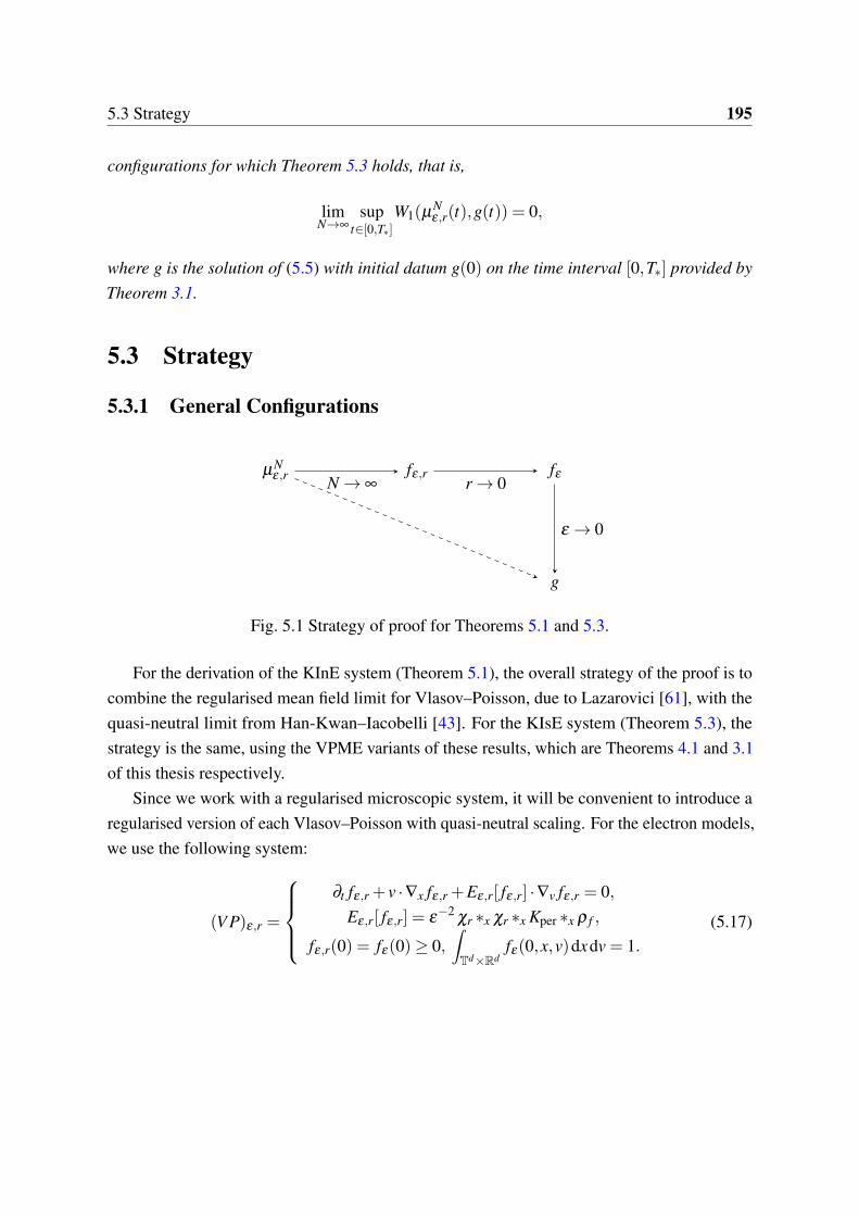
5.3 Strategy 195
configurations for which Theorem 5.3 holds, that is,
limN→∞
supt∈[0,T∗]
W1(µNε,r(t),g(t)) = 0,
where g is the solution of (5.5) with initial datum g(0) on the time interval [0,T∗] provided byTheorem 3.1.
5.3 Strategy
5.3.1 General Configurations
µNε,r fε,r fε
g
N → ∞ r → 0
ε → 0
Fig. 5.1 Strategy of proof for Theorems 5.1 and 5.3.
For the derivation of the KInE system (Theorem 5.1), the overall strategy of the proof is tocombine the regularised mean field limit for Vlasov–Poisson, due to Lazarovici [61], with thequasi-neutral limit from Han-Kwan–Iacobelli [43]. For the KIsE system (Theorem 5.3), thestrategy is the same, using the VPME variants of these results, which are Theorems 4.1 and 3.1of this thesis respectively.
Since we work with a regularised microscopic system, it will be convenient to introduce aregularised version of each Vlasov–Poisson with quasi-neutral scaling. For the electron models,we use the following system:
(V P)ε,r =
∂t fε,r + v ·∇x fε,r +Eε,r[ fε,r] ·∇v fε,r = 0,
Eε,r[ fε,r] = ε−2
χr ∗x χr ∗x Kper ∗x ρ f ,
fε,r(0) = fε(0)≥ 0,∫Td×Rd
fε(0,x,v)dxdv = 1.(5.17)
196 Particle Derivations for Kinetic Euler Systems
For the ion models, we use the following system:
(V PME)ε,r :=
∂t fε,r + v ·∇x fε,r +Eε,r[ fε,r] ·∇v fε,r = 0,
Eε,r =−χr ∗∇Uε,r,
ε2∆Uε,r = eUε,r −χr ∗ρ[ fε,r],
fε,r(0) = fε(0)≥ 0,∫Td×Rd
fε(0,x,v)dxdv = 1.
(5.18)
The strategy is illustrated in Figure 5.1. The steps of the proof are as follows:
(i) With ε and r fixed, we prove the mean field limit for the regularised system. We showthat the empirical measure µN
ε,r coming from the regularised particle system (5.4) or (5.8)converges to the solution fε,r of the regularised Vlasov–Poisson system. The key point isto quantify this convergence in the Wasserstein distance W2.
(ii) With ε fixed, we remove the regularisation from the Vlasov–Poisson system. We showthat the solution fε,r of the regularised system converges, as r tends to zero, to the solutionfε of the Vlasov–Poisson system (5.3) or (1.19). Again we quantify the convergence inW2.
(iii) Finally, we use the known results on the quasi-neutral limit ([43] or Theorem 3.1) toconclude that fε converges to a solution g of the relevant kinetic Euler system, as ε tendsto zero.
The main goal of our estimates is to quantify the rates of convergence in steps (i) and (ii).To do this, we again use an anisotropic distance, as we did in Chapter 4. For some parameter λ ,we consider
W (λ )2 (µ,ν) =
(inf
π∈Π(µ,ν)
∫(Td×Rd)2
λ2|x1 − x2|2 + |v1 − v2|2 dπ(x1,v1,x2,v2)
) 12
.
We then choose λ in order to optimise the rate of convergence we obtain. In this chapter, λ
will be allowed to depend on both ε and r.The estimates for steps (i) and (ii) are performed using similar methods to those used in
Chapter 4. The constants in those estimates depend on L∞(Td) bounds on the mass densitiesρ[ fε,r] and ρ[ fε ]. The main difference for the estimates in this chapter is that we have to keeptrack of how this bound depends on ε . To do this, in the KInE case we use mass densityestimates from [43]. For the KIsE case we proved the necessary estimates in Chapter 3. Werecall these estimates below in Section 5.4.1.3.

5.4 Preliminaries 197
5.3.2 Typicality
Our strategy for the proof of Theorems 5.2 and 5.4 is the same as used in the proof ofTheorem 4.2. We check that, if we choose the initial configurations for the particle systemby drawing independent samples from the reference data fε(0), then the necessary rate ofconvergence (5.14) or (5.15) occurs with high probability.
To prove this, we use the concentration estimates from Fournier–Guillin [29] on the rate ofconvergence of the empirical measures in Wasserstein sense. In comparison to the mean fieldlimit, in this chapter we need to deal with the fact that the reference data fε(0) depend on ε . Itis therefore necessary to keep track of how the constants in the concentration estimate dependon ε . Our strategy is to use the fact that the reference data fε(0) are compactly supported, andto use a scaling argument.
5.4 Preliminaries
5.4.1 Regularised Vlasov–Poisson Systems
5.4.1.1 Existence of Solutions
We need to check that solutions of the regularised Vlasov–Poisson systems exist globallyin time for our choice of initial data fε(0). This follows from the fact that each fε(0) ∈L1∩L∞(Td ×Rd) is compactly supported. For the ion model (5.18), this is proved in Section 2.8of this thesis. For the electron model, we can use the general result for Vlasov equations withLipschitz kernels (Theorem 1.2), since the function χr ∗χr ∗Kper is Lipschitz.
In both cases, since fε,r solves a transport equation with a divergence free field vector field,we have the a priori estimate
supt∈[0,∞)
∥ fε,r(t)∥Lp(Td×Rd) = ∥ fε,r(0)∥Lp(Td×Rd). (5.19)
5.4.1.2 Energy
Each of the regularised systems (5.17) and (5.18) has an associated energy functional. For theelectron model, it is a regularisation of (5.10):
E VPε,r [ f ] :=
∫Td×Rd
|v|2 f dxdv+ε2
2
∫Td
|Eε,r[ f ]|2 dx. (5.20)
198 Particle Derivations for Kinetic Euler Systems
This functional is conserved by solutions fε,r of (5.17):
E VPε,r [ fε,r(t)] = E VP
ε,r [ fε(0)].
For the ion model, we have the following rescaling of (2.58):
E MEε,r [ f ] :=
12
∫Td×Rd
|v|2 f dxdv+ε2
2
∫Td|∇Uε,r|2 dx+
∫Td
Uε,r eUε,r dx.
This functional is conserved by solutions fε,r of (5.18):
E MEε,r [ fε,r(t)] = E ME
ε,r [ fε(0)].
The conservation of these functionals implies a uniform-in-time a priori bound on ∥ρ[ f ]∥L
d+2d (Td)
for a solution f of one of the regularised Vlasov–Poisson systems. For the electron model, thisfollows from the fact that both terms in (5.20) are non-negative. Thus if E VP
ε,r [ f ]≤C0, then wehave an upper bound on the second moment∫
Td×Rd|v|2 f dxdv ≤C0.
For the ion model, since xex ≥−e−1, we have a similar estimate: if E MEε,r [ f ]≤C0, then∫
Td×Rd|v|2 f dxdv ≤C0 + e−1.
It then follows from the interpolation estimate in Lemma 1.12 that
∥ρ[ f ]∥L
d+2d (Td)
≤C1, (5.21)
where C1 depends on C0 and ∥ f∥L∞(Td×Rd).For solutions fε,r of the regularised Vlasov–Poisson systems, the uniform Lp(Td ×Rd)
estimate (5.19) on fε,r then implies that ∥ρ[ fε,r]∥L
d+2d (Td)
is bounded uniformly in time for
solutions of the regularised Vlasov–Poisson systems.
5.4 Preliminaries 199
5.4.1.3 Mass Bounds
In our proofs, we will need uniform estimates on the mass density. That is, we use a bound ofthe form
supt∈[0,T ]
∥ρ[ fε(t)]∥L∞(Td) ≤ Mε,T , supr
supt∈[0,T ]
∥ρ[ fε(t)]∥L∞(Td) ≤ Mε,T . (5.22)
For the classical Vlasov–Poisson system, we can obtain these estimates from [43]. Theseresults are based on controlling the growth of the size of the support of fε(t) over time, in thestyle of Batt and Rein [10], quantifying the dependence on ε . We use the following result.
Proposition 5.5. Let d = 2,3. Let fε be a solution of the Vlasov–Poisson system (5.3), forinitial data satisfying Assumption 2. Fix T > 0. Then there exists Cd,T such that for all t ∈ [0,T ],
∥ρ[ fε ]∥L∞(Td) ≤Cd,T ε−dζ .
where ζ is defined in (5.12)-(5.13).
The same estimate applies to the density ρ[ fε,r] for solutions of the regularised system(5.17).
For the VPME system, we use estimates from Chapter 3, in particular Proposition 3.10.Again the same estimates apply to the solution of the regularised system (5.18).
Proposition 5.6. Let d = 2,3. Let fε(0) ∈ L1 ∩L∞(Td ×Rd) be compactly supported, withsupport contained in Td ×BR(0), where R ≤ eAε−2
for some constant A. Then there existsC =C(A,d) depending on A and d and CT depending on T such that
supt∈[0,T ]
∥ρ fε (t)∥L∞(Td) ≤CT eCε−2.
5.4.1.4 Empirical measures
Note that, if (Xi(t),Vi(t))Ni=1 is a solution of the extended electrons systems (5.4), then the
resulting empirical measure µNε,r, defined by (5.9), is a weak solution of the regularised Vlasov–
Poisson system (5.17). A similar property holds for (5.8) and the regularised VPME system(5.18).
200 Particle Derivations for Kinetic Euler Systems
5.4.2 Filtering
In the derivation of KInE, convergence holds for a version of the empirical measure filteredusing the corrector function Rε . In our estimates, we will need to account for the effect of thefiltering on the Wasserstein distance. For this we quote the following lemma from [43]:
Lemma 5.7. Let ν1,ν2 be probability measures on Td ×Rd , and let νi denote a measureobtained by filtering νi using a given vector field R : Td → Rd (see Definition 5). Then
W1(ν1, ν2)≤ (1+∥∇xR∥L∞)W1(ν1,ν2).
In this chapter we will always use the corrector Rε defined by (1.53). In this case
|∇xRε | ≤ |∇xd+|+ |∇xd−|.
Thus there exists CT independent of ε such that for t ∈ [0,T ],
∥∇xRε∥L∞(Td) ≤CT .
ThusW1(ν1, ν2)≤CTW1(ν1,ν2).
5.4.3 Quasi-neutral Limit for Classical Vlasov–Poisson
We recall the quasi-neutral limit for the classical Vlasov–Poisson system proved in [43, Theorem1].
Theorem 5.8. Let γ , δ0, and C0 be positive constants, with δ0 > 1. Consider a choice fε(0)of non-negative initial data in L1 satisfying Assumption 2. For all ε ∈ (0,1), consider fε(t)a global weak solution of (V P)ε with initial condition fε(0). Define the filtered distributionfunction
fε(t,x,v) := fε
(t,x,v−Rε)
)where Rε is the corrector defined in (1.53).
There exist T > 0 and g(t) a weak solution on [0,T ] of (KIE) with initial condition g0 suchthat
limε→0
supt∈[0,T ]
W1( fε(t),g(t)) = 0.

5.5 Proof for General Configurations 201
5.5 Proof for General Configurations
5.5.1 Stability for the Regularised Vlasov–Poisson Systems
In this section we prove a quantitative estimate of the rate of convergence of the empiricalmeasure of the solution µN
ε,r of the scaled and regularised N-particle system (5.4), to the solutionfε,r of the mean-field regularised equation (5.17). Our approach is similar to the methods of[61].
Proposition 5.9. Fix T > 0. For any small β > 0, there exists Cβ ,T such that the followingholds: Let fε,r be a solution of (5.17) and µN
ε,r be defined as in (1.58). Let ε = εN , r = rN bechosen such that
r < e−Cβ ,T ε−2−dζ
(5.23)
Assume that the initial condition for (5.4) is ‘well-placed’ in the sense that there exists η > β
such that
limN→∞
W2(µNε,r(0), fε(0))
ε−γr1+d/2+η/2 = 0. (5.24)
Then for any η ′ ∈ (β ,η), there exists a constant C = C(β ,T,η ,η ′,γ,ζ ) such that for all Nsufficiently large, for all t ≤ T we have
W 22 (µ
Nε,r(t), fε,r(t))≤Crd+2+η ′−β .
Proof. We follow the proof of Lemma 4.8, with a quasi-neutral scaling. To lighten the notation,we drop the sub- and superscripts r,ε,N from fε,r and µN
ε,r. We define a coupling πt that followsthe characteristic flows associated to f and µ:
X1 =V1
V1 = E(µ)ε,r (X1)
(Z1(0;0,z)) = z = (x,v)
E(µ)ε,r =−χr ∗∇U (µ)
ε,r
ε2∆U (µ)ε,r = eU (µ)
ε,r −χr ∗ρµ
X2 =V2
V2 = E( f )ε,r (X2)
(Z2(0;0,z)) = z = (x,v)
E( f )ε,r =−χr ∗∇U ( f )
ε,r
ε2∆U ( f )ε,r = eU ( f )
ε,r −χr ∗ρ f .
These systems have unique classical solutions by the same arguments as in the proof ofLemma 4.8.
Fixing an arbitrary coupling of the initial data π0 ∈ Π(µ0, f0), we define a coupling πt ∈Π(µ(t), f (t)) by
πt = (Z1(t;0, ·)⊗Z2(t;0, ·))# π0. (5.25)

202 Particle Derivations for Kinetic Euler Systems
Using πt , we define an anisotropic functional D. For λ > 0, let
D(t) =∫(Td×Rd)2
λ2|x1 − x2|2 + |v1 − v2|2 dπt(x1,v1,x2,v2). (5.26)
We perform a Grönwall estimate on D. Following the same steps as in the proof ofLemma 4.8, we obtain
D ≤ (α +λ )D+Cα
2
∑i=1
Ii,
where
I1 :=∫
|E(µ)ε,r (X
(1)t )−E(µ)
ε,r (X(2)t )|2 dπ0, I2 :=
∫|E( f )
ε,r (X(2)t )−E(µ)
ε,r (X(2)t )|2 dπ0.
I1 and I2 are estimated in the same way as in the proof of Lemma 4.8, which follows theargument of [61]. Compared to the case ε = 1, here we gain an extra factor of ε−4 due to thequasi-neutral scaling. The estimates are otherwise the same. We obtain
D ≤ (λ +α)D+ε−4
4αC(1+ | logr|)2
(M+ r−(d+2)
λ−2D
)2λ−2D. (5.27)
We introduce the truncated functional
D = 1∧(
r−(d+2)λ−2D
).
By the same argument as in the proof of Lemma 4.8, D is Lipschitz and therefore differentiablealmost everywhere and absolutely continuous, with either
ddt
D(t) = 0 orddt
D(t) = r−(d+2)λ−2 d
dtD(t).
Thus (5.27) implies that, for almost all t,
ddt
D ≤ (λ +α)D+Cε−4
αM2| logr|2λ
−2D.
We then optimise the exponent by choosing
α∗ =Cdε−2(1+ | logr|)Mλ
−1∗ , λ∗ =Cdε
−1(1+ | logr|)1/2√
M.
Thenddt
D ≤Cdλ∗D.
5.5 Proof for General Configurations 203
Since D is absolutely continuous, the integrated form of this inequality also holds. Then byGrönwall’s inequality we deduce the following estimate:
sup[0,T ]
D(t)≤ exp(Cdλ∗T )D(0). (5.28)
Now we must choose r and ε in such a way as to prevent the factor exp(Cdλ∗T ) fromexploding too quickly.
First we check that infπ0 D(0)→ 0. For convenience we will define a function ω by
ω(N) =W2(µ
Nε (0), fε(0))
ε−γr1+d/2+η/2 ;
thus (5.24) implies that ω is bounded. Recalling (4.22),
infπ0
D(0)≤ 12
λ2W 2
2 (µNε (0), fε(0)).
Thus, since by definition D(0)≤ λ−2r−(d+2)D(0), it follows that
infπ0
D(0)≤ 12
r−(d+2)W 22 (µ
Nε (0), fε(0)).
By definition of ω we have
infπ0
D(0)≤ 12
rηε−2γ
ω(N)2.
If (5.23) holds, then ε−1 ≤Cβ ,T | logr|1
2+dζ and thus
infπ0
D(0)≤Crη | logr|2γ
2+dζ ω(N)2.
Then for any η ′ < η there exists C =Cβ ,T,η ′,γ,ζ such that
infπ0
D(0)≤Crη ′.
Next, we use the Gronwall estimate to get convergence at later times. We can do this bycontrolling the exponential growth factor in (5.28). Observe that for r < 1 this factor satisfies
eCM1/2ε−1| logr|1/2T = r−CM1/2ε−1| logr|−1/2T . (5.29)
204 Particle Derivations for Kinetic Euler Systems
If ε,r satisfy (5.23), then by Proposition 5.5,
CM1/2ε−1| logr|−1/2T ≤CT ε
−1− dζ
2 | logr|−1/2 ≤ β (5.30)
and hencer−CM1/2ε−1| logr|−1/2T ≤ r−β . (5.31)
This implies that for all t ∈ [0,T ]
infπ0
D(t)≤ infπ0
D(0)r−β
≤Crη ′−β . (5.32)
Upon choosing η ′ > β , we find that infπ0 D(T )→ 0 as N → ∞.For N sufficiently large, we have infπ0 D(T )< 1. Then
sup[0,T ]
W 22 ( fε,r,µ
Nε,r)≤ λ
2rd+2 infπ0
D(T ). (5.33)
Recall that we chose λ =CM1/2ε−1| logr|1/2. Thus by (5.30) we have λ ≤CβT−1| logr|.Hence
λ2rd+2 ≤Cβ ,T | logr|2rd+2.
Then by combining (5.33) with (5.32) and (5.33) we obtain
sup[0,T ]
W 22 ( fε,r,µ
Nε,r)≤C| logr|2rd+2+η ′−β .
By adjusting η ′ and C so as to absorb the logarithmic factor, we may conclude that for Nsufficiently large,
sup[0,T ]
W 22 ( fε,r,µ
Nε,r)≤Crd+2+η ′−β .
5.5.2 Stability for Regularised VPME
The following lemma is a quantified version of Lemma 4.8.
Lemma 5.10 (Weak-strong stability for the regularised equation, with quasineutral scaling).Let fε(0) satisfy the assumptions of Theorem 3.1. Let fε,r be the solution of (5.18) with datafε(0). Fix any T > 0. Then there exists a constant A depending on T and fε(0) such that the
5.5 Proof for General Configurations 205
following holds. For each (ε,r), let µε,r be a measure solution of (5.18). Assume that for someη > 0, r = r(ε) satisfies
r ≤[exp3(Aε
−2)]−1
and limr→0
W2 (µε,r(0), fε(0))r(d+2+η)/2
= 0. (5.34)
Thenlimr→0
supt∈[0,T ]
W2 (µε,r(t), fε,r(t)) = 0.
Proof. We follow the proof of Lemma 4.8, tracking the dependence of the constants on ε . Forease of notation we drop the subscripts on fε,r and µε,r. Let πt be defined as in (5.25), and letD be defined as in (5.26). Following the same steps as for Lemma 4.8, we obtain
D ≤ (α +λ )D+Cα
4
∑i=1
Ii,
where
I1 :=∫
|E(µ)ε,r (X
(1)t )− E(µ)
ε,r (X(2)t )|2 dπ0, I2 :=
∫|E( f )
ε,r (X(2)t )− E(µ)
ε,r (X(2)t )|2 dπ0,
I3 :=∫
|E(µ)ε,r (X
(1)t )− E(µ)
ε,r (X(2)t )|2 dπ0, I4 :=
∫|E( f )
ε,r (X(2)t )− E(µ)
ε,r (X(2)t )|2 dπ0.
To estimate these quantities, we first note some basic Lp(Td) estimates on the regularisedmass density χr ∗ρµ , using (4.23). For p = d+2
d , since fε(0) has uniformly bounded energy(1.66), by (5.21) we obtain
∥ρ f ∥L
d+2d (Td)
≤C,
where C depends on C0 and d only. Thus
∥χr ∗ρµ∥L
d+2d (Td)
≤Cd
(1+ r−(d+2)
λ−2D
), (5.35)
for Cd depending on C0 and d.For p = ∞ we obtain
∥χr ∗ρµ∥L∞(Td) ≤Cd
(Mε,T + r−(d+2)
λ−2D
). (5.36)
where Mε,T is a constant such that
supt∈[0,T ]
∥ρ ft∥L∞(Td) ≤ Mε,T .
206 Particle Derivations for Kinetic Euler Systems
By Proposition 5.6, there exists a constant C depending on T such that
supt∈[0,T ]
∥ρ ft∥L∞(Td) ≤ exp(Cε−2).
Therefore Mε,T may be chosen to satisfy
Mε,T ≤ exp(Cε−2). (5.37)
We estimate I1 as in (4.27). An extra factor of ε−4 appears due to the quasineutral scalingon the force:
I1 ≤Cε−4(logr)2
(Mε,T + r−(d+2)
λ−2D
)2λ−2D.
Similarly, I2 is estimated as in (4.28) using Lemma 2.10 and (5.36) to obtain
I2 ≤Cε−4Mε,T (Mε,T + r−(d+2)
λ−2D)λ−2D.
For I3 the same computation as in (4.29) implies that
I3 ≤∫(Td×Rd)2
∥U (µ)ε,r ∥2
C2(Td)|x− y|2 dπt .
Using (5.35) we apply Proposition 3.3, which is a regularity estimate on U (µ)ε,r , taking account
of the quasi-neutral scaling, to obtain
∥U (µ)ε,r ∥C2(Td) ≤Cd exp2
(Cdε
−2(
1+ r−(d+2)λ−2D
)).
Thus
I3 ≤C exp2
[Cdε
−2(1+ r−(d+2)λ−2D)
]∫(Td×Rd)2
|x− y|2 dπt
≤C exp2
[Cdε
−2(1+ r−(d+2)λ−2D)
]λ−2D.
For I4, as in (4.30) we obtain
I4 ≤ ∥ρ f ∥L∞(Td)∥∇U ( f )ε,r −∇U (µ)
ε,r ∥2L2(Td).
5.5 Proof for General Configurations 207
By the stability estimate from Lemma 3.8 and the density bound (5.36),
∥∇U ( f )ε,r −∇U (µ)
ε,r ∥2L2(Td) ≤Cε
−2 exp2
[Cd ε
−2(1+ r−(d+2)λ−2D)
]∥U ( f )
ε,r −U (µ)ε,r ∥2
L2(Td)
≤Cε−6 exp2
[Cd ε
−2(1+ r−(d+2)λ−2D)
](Mε,T + r−(d+2)
λ−2D)λ−2D.
Thus
I4 ≤Cε−6Mε,T exp2
[Cdε
−2(1+ r−(d+2)λ−2D)
](Mε,T + r−(d+2)
λ−2D)λ−2D.
We summarise this as
D ≤ (λ +α)D+1α
Cε−4(1+ | logr|)2
(Mε,T + r−(d+2)
λ−2D
)2λ−2D (5.38)
+Cexp2
[Cdε
−2(1+ r−(d+2)λ−2D)
](1+Mε,T (Mε,T + r−(d+2)
λ−2D)
)λ−2D.
We introduce the truncated functional
D = 1∧(
r−(d+2)λ−2D
),
which is Lipschitz and so differentiable almost everywhere. Where the derivative exists, (5.38)implies that
ddt
D ≤ (λ +α)D+1
4αCd
[ε−4 (1+ | logr|)2 + exp2(Cε
−2)]
M2ε,T λ
−2D.
We optimise the exponent by choosing
α∗ =Cd
[ε−4 (1+ | logr|)2 + exp2(Cε
−2)]1/2
Mε,T λ−1∗
λ∗ =Cd
[ε−4 (1+ | logr|)2 + exp2(Cε
−2)]1/4√
Mε,T . (5.39)
Thenddt
D ≤Cdλ∗D.
By absolute continuity of D, it follows that
D(t)≤ D(0)+Cdλ∗
∫ t
0D(s)ds.
208 Particle Derivations for Kinetic Euler Systems
From this we deduce that
sup[0,T ]
D(t)≤ exp(Cdλ∗T )D(0)
≤ r−(d+2)λ−2∗ exp(Cdλ∗T )D(0)
≤ r−(d+2) exp(Cdλ∗T )D(0)
≤Cd exp[| logr|
((d +2)+CdT
√Mε,T ε
−1| logr|−1/2)+√
Mε,T exp2(Cε−2)]D(0).
By the estimate (5.37) on Mε,T , we obtain
sup[0,T ]
D(t)≤Cd exp[| logr|
((d +2)+CdT exp(Cε
−2)| logr|−1/2)]
exp3(Cε−2)D(0).
By assumption (5.34) on the relationship between ε and r,
| logr|−1/2 ≤ exp[−1
2exp(Aε
−2)
].
Thus we have
sup[0,T ]
D(t)≤Cd exp[| logr|
((d +2)+ exp(Cε
−2 − 12
exp(Aε−2))
)]exp3(Cε
−2)D(0).
By assumption on W2(µNε,r(0), fε,r(0)), for all sufficiently small r there exists a choice of initial
coupling π(r)0 such that
D(0)< rd+2+η .
Then
sup[0,T ]
D(t)≤Cd exp[| logr|
(exp(Cε
−2 − 12
exp(Aε−2))−η
)+ exp2(Cε
−2)
].
For sufficiently small ε ,
sup[0,T ]
D(t)≤Cd exp[−1
2η | logr|+ exp2(Cε
−2)
]≤Cd exp
[−1
2η exp2(Aε
−2)+ exp2(Cε−2)
].
5.5 Proof for General Configurations 209
Thus if A >C, thensup[0,T ]
D(t)→ 0
as ε tends to zero. In particular, for ε sufficiently small,
infπ0
supt∈[0,T ]
D(t)< 1.
Hence, for ε sufficiently small,
infπ0
supt∈[0,T ]
D(t) = infπ0
supt∈[0,T ]
r−(d+2)λ−2∗ D(t).
Thus
supt∈[0,T ]
W 22 (µ
Nε,r(t), fε,r(t))≤ inf
π0sup
t∈[0,T ]D(t) = rd+2
λ2∗ inf
π0sup
t∈[0,T ]D(t)≤ rd+2
λ2∗ .
By (5.39),
λ2∗ =Cd
[ε−4 (1+ | logr|)2 + exp2(Cε
−2)]1/2
exp(Cε−2).
Hence, for any α > 0,
rd+2λ
2∗ ≤Crd+2−α exp2(Cε
−2)≤C exp
exp(Cε−2)− (d +2−α)exp2(Aε
−2).
The right hand side converges to zero as ε tends to zero. Therefore
limε→0
supt∈[0,T ]
W 22 ( ft ,µt) = 0.
5.5.3 Removal of the Regularisation
5.5.3.1 Classical Vlasov–Poisson
In this section, we prove the following Gronwall-type estimate between solutions of theregularised and unregularised Vlasov-Poisson systems.
Proposition 5.11. (i) Let fε,r be a solution of (5.17) and fε a solution of (5.3), both havingthe same initial datum fε(0). Let M = Mε,T be chosen such that (5.22) is satisfied. Then
210 Particle Derivations for Kinetic Euler Systems
there exists a constant C, independent of r, M and ε , such that for all t ∈ [0,T ]
W2( fε,r(t), fε(t))≤Cε−3/2M3/4r| logr|−1/4eCε−1M1/2| logr|1/2t .
(ii) Let fε(0) be a set of initial data satisfying Assumption 2. Let ζ be defined as in (5.12)-(5.13), and let T > 0 be fixed. If ε = εN and r = rN are chosen to satisfy (5.23) for someβ < 1, then
limN→∞
supt∈[0,T ]
W2( fε,r(t), fε(t)) = 0. (5.40)
Proof. We consider couplings of fε,r and fε that evolve along the characteristic flows oftheir respective equations. Since fε,r and fε have the same initial datum fε(0), the choiceπ0(x,v,y,w) = f0(x,v)δ (x− y,v−w) is an optimal initial coupling, so that at time t = 0 wehave
W 22 ( fε,r, fε) =
∫(Td×Rd)2
|x− y|2 + |v−w|2 dπ0(x,v,y,w)
We take πt to solve
(∂t + v ·∇x +w ·∇y)πt +(Eε,r[ fε,r](x) ·∇v +Eε [ fε ](y) ·∇w)πt = 0.
Then πt is a coupling of fε,r(t) and fε(t) for all times t. As before we define an anisotropicdistance D: let
D(t) =12
∫(Td×Rd)2
λ2|x− y|2 + |v−w|2 dπt(x,v,y,w)
for some λ to be specified later. Then, as in the proof of Lemma 4.8, we estimate that
D′(t)≤ (λ +α)D(t)+1
2α
∫(Td×Rd)2
|Eε,r[ fε,r](x)−Eε [ fε ](y)|2 dπt . (5.41)
By the triangle inequality, the second term in (5.41) may be estimated as follows:
12α
∫(Td×Rd)2
|Eε,r[ fε,r](x)−Eε [ fε ](y)|2 dπt ≤1α
∫(Td×Rd)2
|Eε,r[ fε,r](x)−Eε,r[ fε,r](y)|2 dπt︸ ︷︷ ︸:=I1
+1α
∫(Td×Rd)2
|Eε,r[ fε,r](y)−Eε [ fε ](y)|2 dπt︸ ︷︷ ︸:=I2
.
The term I1 is estimated using the Lipschitz regularity of the regularised forces (Lemma4.6):
5.5 Proof for General Configurations 211
I1 =∫(Td×Rd)2
|Eε,r[ fε,r](x)−Eε,r[ fε,r](y)|2 dπ
≤∫(Td×Rd)2
∥ε−2
χr ∗Kper ∗ (χr ∗ρ fε,r)∥2Lip |x− y|2 dπ
≤Cε−4| logr|2(1+∥χr ∗ρ fε,r∥L∞)2
∫(Td×Rd)2
|x− y|2 dπ
≤Cε−4| logr|2M2
λ−2D(t).
For I2, we first observe that since the y-marginal of πt is ρ fε (y)dy,
I2 =∫Td
|ε−2Kper ∗ (χr ∗χr ∗ρ fε,r −ρ fε )|2(y)ρ fε (y)dy
≤ M∥ε−2Kper ∗ (χr ∗χr ∗ρ fε,r −ρ fε )∥
2L2(Td), (5.42)
where (5.42) follows from the fact that ∥ρ fε∥L∞ ≤ M by definition (recall (5.22)).We then apply the Loeper stability estimate, Theorem 1.17:
∥ε−2Kper ∗ (χr ∗χr ∗ρ fε,r −ρ fε )∥L2(Td) ≤ ε
−2M1/2W2(χr ∗χr ∗ρ fε,r ,ρ fε ).
To control the Wasserstein distance we first apply the triangle inequality:
W2(χr ∗χr ∗ρ fε,r ,ρ fε )≤W2(χr ∗χr ∗ρ fε,r ,χr ∗ρ fε,r)+W2(χr ∗ρ fε,r ,ρ fε,r)+W2(ρ fε,r ,ρ fε ).
The third term can be controlled by λ−1D1/2 due to (4.21). We apply Lemma 4.4 to eachof the first two terms. This results in the estimate
W2(χr ∗χr ∗ρ fε,r ,ρ fε )≤ 2r+λ−1D1/2.
Thus we get the following estimate for I2:
I2 ≤Cε−4M2(2r+λ
−1D1/2)2
≤Cε−4M2(r2 +λ
−2D).

212 Particle Derivations for Kinetic Euler Systems
Substituting these estimates into (5.41) gives us that
D′(t)≤[
λ +α +1α
Cε−4M2(| logr|2 +1)λ−2
]D(t)+
Cα
ε−4M2r2
≤[
λ +α +1α
Cε−4M2| logr|2λ
−2]
D(t)+Cα
ε−4M2r2. (5.43)
We will now choose the parameters α and λ so as to minimise the constant in the exponentialpart of our Gronwall estimate; that is, the coefficient of D in (5.43). This has a minimum for(α,λ ) satisfying α = Cλ−1ε−2M| logr|
λ =(
Cε−4M2| logr|2α
)1/3,
that is, α = λ =Cε−1M1/2| logr|1/2. With this choice of parameters (5.43) becomes
D′(t)≤Cε−1M1/2| logr|1/2D(t)+Cε
−3M3/2r2| logr|−1/2.
Since D(0) = 0, the above inequality implies that
D(t)≤Cε−3M3/2r2| logr|−1/2eCε−1M1/2| logr|1/2t .
We conclude that
W2( fε,r(t), fε(t))≤Cε−3/2M3/4r| logr|−1/4eCε−1M1/2| logr|1/2t .
Finally, we use this to prove (5.40). Since fε(0) are assumed to satisfy Assumption 2,we may apply Proposition 5.5 to deduce that
M ≤Cε−ζ d,
for ζ defined in (5.12)-(5.13). Next, we observe that the relation (5.23) implies that
ε−(2+ζ d) ≤CT,β | logr|,
for some Cβ ,T . Thusε−1M1/2 ≤Cβ ,T | logr|1/2.
5.5 Proof for General Configurations 213
Moreover, by (5.29) and (5.31), we have
eCε−1M1/2| logr|1/2t ≤ r−β .
Thussup
t∈[0,T ]W2( fε,r(t), fε(t))≤CT r1−β | logr|1/2.
Since β < 1, the right hand side converges to 0 as N → ∞. This completes the proof.
5.5.3.2 VPME
The next lemma is a quantified version of Lemma 4.9.
Lemma 5.12 (Approximation of (VPME) in quasineutral scaling). Let fε(0) satisfy the as-sumptions of Theorem 3.1. Let fε,r be the solution of the scaled and regularised Vlasov equation(5.18) with initial datum fε(0). Let fε be the unique bounded density solution of (3.1).
Fix T > 0. Then there exists a constant C depending on T and on fε(0)ε such that thefollowing holds. If r and ε satisfy
r ≤[exp3(Cε
−2)]−1
,
thenlimr→0
sup[0,T ]
W2 ( fε,r(t), fε(t)) = 0.
Proof. By (1.66), Lemma 1.12 and (5.21) there exists a constant C depending on C0 and d onlysuch that
∥ρf (r)ε
∥L∞([0,T ];L
d+2d (Td))
,∥ρ fε∥L∞([0,T ];Ld+2
d (Td))≤C. (5.44)
By Proposition 3.10, there exists a constant C depending on the initial data and T such that
∥ρf (r)ε
∥L∞([0,T ];L∞(Td)),∥ρ fε∥L∞([0,T ];L∞(Td)) ≤ exp(Cε−2). (5.45)
We will control the Wasserstein distance between fε,r and fε using a particular couplingπt . Since both solutions share the same initial datum, we take π0 to be the trivial couplingfε(0)(x,v)δ ((x,v)− (y,w))dxdvdydw. We construct πt ∈ Π( fε(t), fε,r(t)) as in (2.25), using

214 Particle Derivations for Kinetic Euler Systems
the scaled version of the characteristic systems in (4.35):
X (1)x,v =V (1)
x,v
V (1)x,v = E(X (1)
x,v )
(X (1)x,v (0),V
(1)x,v (0)) = (x,v)
E =−∇U
ε2∆U = eU −ρ fε
X (2)x,v =V (2)
x,v
V (2)x,v = Er(X
(2)x,v )
(X (2)x,v (0),V
(2)x,v (0)) = (x,v)
Er =−χr ∗∇Ur
ε2∆Ur = eUr −χr ∗ρ fε,r .
We define D as in (4.19). As in Lemma 4.8, we obtain for any α > 0,
D ≤ (α +λ )D+Cα
5
∑i=1
Ii,
where
I1 :=∫
|∇Ur(X(1)t )−∇Ur(X
(2)t )|2 dπ0, I2 :=
∫|∇Ur(X
(1)t )−∇U(X (1)
t )|2 dπ0,
I3 :=∫
|∇Ur(X(1)t )−∇Ur(X
(2)t )|2 dπ0, I4 :=
∫|∇U(X (1)
t )−∇Ur(X(1)t )|2 dπ0
I5 :=∫
|χr ∗∇Ur(X(2)t )−∇Ur(X
(2)t )|2 dπ0.
I1 is estimated as in (4.36). There is an extra factor of ε−4 due to the quasineutral scalingand the mass bound M = Mε,T depends on ε:
I1 ≤Cε−4| logr|2M2
ε,T λ−2D.
We estimate I2 as in (4.37), keeping track of the dependence on ε in Lemma 2.10:
∥∇U −∇Ur∥L2(Td) ≤Cε−2√Mε,T (r+λ
−1√
D).
We conclude thatI2 ≤Cε
−4M2ε,T (r+λ
−1√
D)2.
For I3, by the regularity estimate from Proposition 2.4 and the uniform Ld+2
d (Td) estimateon the density (5.44) we have
∥Ur∥C2,α (Td) ≤ exp2(Cε−2),

5.5 Proof for General Configurations 215
where C depends only on C0. We obtain
I3 ≤ exp2(Cε−2)
∫Td×Rd
|X (1)t −X (2)
t |2 dπ0
≤ exp2(Cε−2)λ
−2D.
For I4 we use the stability estimate from Lemma 3.6 and the Ld+2
d (Td) estimate (5.44):
∥∇U −∇Ur∥L2(Td) ≤ exp2(Cε−2)∥∇U −∇Ur∥L2(Td) ≤ exp2(Cε
−2)√
Mε,T (r+λ−1√
D).
HenceI4 ≤ exp2(Cε
−2)M2ε,T (r+λ
−1√
D)2.
For I5, by (4.38) we have
∥χr ∗∇Ur −∇Ur∥2L2(Td) ≤Cr2∥Ur∥2
W 2,2(Td).
Thus
I5 :=∫Td
|χr ∗∇Ur(x)−∇Ur(x)|2 ρf (r)ε
(dx)
≤ ∥ρf (r)ε
∥L∞(Td)∥χr ∗∇Ur −∇Ur∥2L2(Td)
≤Cr2Mε,T∥Ur∥2W 2,2(Td)
≤Cr2ε−4Mε,T∥eUr −ρ
f (r)ε
∥2L2(Td).
As in (4.39), we have
∥ρ fε,r∥L2(Td) ≤ ∥ρ fε,r∥d−22d
L∞(Td)∥ρ fε,r∥
d+22d
Ld+2
d (Td)≤CM
d−22d
ε,T .
To estimate eUr , first note that by Proposition 2.4 and (5.44),
∥Ur∥L∞(Td) ≤Cε−2.
By (3.8),∥eUr∥L2(Td) ≤ exp(Cε
−2).
Thus∥eUr∥L2(Td) ≤C exp
(∥Ur∥L∞(Td)
)∥eUr∥L2(Td) ≤ exp(Cε
−2).

216 Particle Derivations for Kinetic Euler Systems
Therefore
I5 ≤Cr2ε−4Mε,T
(M
d−2d
ε,T + eCε−2).
Putting these five estimates together, we obtain
D ≤ (α +λ )D+C
αλ 2 r2exp2(Cε−2)M2
ε,T
+C
αλ 2
exp2(Cε
−2)M2ε,T + ε
−4| logr|2M2ε,T + exp2(Cε
−2)
D.
By (5.45), we may estimate that
Mε,T ≤ exp(Cε−2).
From this we deduce
D ≤ (α +λ )D+C
αλ 2
exp(Cε
−2)| logr|2 + exp2(Cε−2)
D+C
αλ 2 exp2(Cε−2)r2.
After choosing α and λ so as to minimise the constant in front of D we obtain
D ≤Cλ∗D+ exp2(Cε−2)r2,
whereλ∗ =
[exp(Cε
−2)| logr|2 + exp2(Cε−2)]1/4 ≥ 1,
for r,ε sufficiently small.Therefore, by a Grönwall estimate
D(t)≤(D(0)+ exp2(Cε
−2)r2)exp [Ctλ∗].
Since π0 was trivial, D(0) = 0. Since D controls the squared Wasserstein distance,
W 22 ( fε,r(t), fε(t))≤ exp(Cε
−2)r2 exp [Ctλ∗].
Then, by definition of λ∗,
supt∈[0,T ]
W 22 ( fε,r(t), fε(t))≤ r2 exp
[exp(CT ε
−2)| logr|1/2]· exp3(CT ε
−2).
5.5 Proof for General Configurations 217
If r ≤[exp3(Aε−2)
]−1, then
eCε−2| logr|−1/2 ≤ exp
[CT ε
−2 − 12
exp(Aε−2)
]→ 0
as ε tends to zero, for any A ≥ 0. Hence, for any η > 0, for ε sufficiently small,
r2 exp[exp(CT ε
−2)| logr|1/2]≤ r2−exp(CT ε−2)| logr|−1/2
≤ r2−η .
Moreover,
r2−η exp3(CT ε−2)≤ exp
[exp2(CT ε
−2)− (2−η)exp2(Aε−2)],
which converges to zero for any η < 2 as ε tends to zero, as long as A ≥CT .Therefore, if r ≤
[exp3(Aε−2)
]−1 for A ≥CT , then as ε tends to zero (and so r also tendsto zero),
supt∈[0,T ]
W2( fε,r(t), fε(t))→ 0.
5.5.4 Conclusion of the Proof
5.5.4.1 From Extended Electrons to KInE
We combine the previous results to complete the proof of Theorem 5.1. We use µ to denotethe distribution produced by filtering µ using the correctors defined in (1.53), followingDefinition 5.
Proof of Theorem 5.1. In the following, µNε,r denotes the empirical measure associated to
the solution of the particle system (5.4), while fε,r denotes the solution of the regularisedVlasov–Poisson system (5.17) with initial datum fε(0). fε denotes the solution of the scaledVlasov–Poisson system (5.3) with initial datum fε(0). Let g be the solution of the KInEsystem (5.1), on some time interval [0,T∗], obtained in the quasineutral limit from fε usingTheorem 5.8.
Our aim is to estimate W1(µNε,r,g). First, we apply the triangle inequality for the Wasserstein
distance to getW1(µ
Nε,r,g)≤W1(µ
Nε,r, fε)+W1( fε ,g)
218 Particle Derivations for Kinetic Euler Systems
We begin by estimating W1(µNε,r, fε). By Lemma 5.7 and the fact that W1 ≤W2,
sup[0,T ]
W1(µNε,r, fε)≤CT sup
[0,T ]W1(µ
Nε,r, fε)
≤CT sup[0,T ]
W2(µNε,r, fε)
≤CT
(sup[0,T ]
W2(µNε,r, fε,r)+ sup
[0,T ]W2( fε,r, fε)
).
Under conditions (5.24) and (5.23), the first term converges to zero by Proposition 5.9. Thesecond term converges by Proposition 5.11. Hence
limN→∞
sup[0,T ]
W1(µNε,r, fε) = 0.
For W1( fε ,g), we apply Theorem 5.8 to deduce that
limN→∞
sup[0,T ]
W1( fε ,g) = 0.
Thereforelim
N→∞sup[0,T ]
W1(µNε,r,g) = 0.
5.5.4.2 From Extended Ions to KIsE
Proof of Theorem 5.3. In the following, µNε,r denotes the empirical measure associated to the
solution of the particle system (5.8), while fε,r denotes the solution of the scaled version of(5.18) with initial datum fε(0). fε denotes the solution of the scaled VPME system (5.7) withinitial datum fε(0). Let g be the solution of the KIE system (3.2), on some time interval [0,T∗],obtained in the quasineutral limit from fε using Theorem 3.1.
Our aim is to estimate W1(µNε,r(t),g(t)). By the triangle inequality for W1,
supt∈[0,T∗]
W1(µNε,r(t),g(t))≤ sup
t∈[0,T∗]W1(µ
Nε,r(t), fε,r(t))
+ supt∈[0,T∗]
W1( fε,r(t), fε(t))+ supt∈[0,T∗]
W1( fε(t),g(t)). (5.46)
The last term converges to zero as ε tends to zero, by Theorem 3.1.
5.6 Typicality 219
For the other two terms, we first observe that
W1(µNε,r(t), fε,r(t))≤W2(µ
Nε,r(t), fε,r(t)), W1( fε,r(t), fε(t))≤W2( fε,r(t), fε(t)).
Then the second term of (5.46) converges to zero by Lemma 5.10 and the third term of (5.46)converges to zero by Lemma 5.12, provided that (5.34) is satisfied for C depending on T∗.
5.6 Typicality
5.6.1 Concentration Estimates
To prove the typicality theorems - Theorem 5.2 and Theorem 5.4, we use the same strategy asin Section 4.6. We employ concentration estimates, due to Fournier and Guillin [29], that allowus to quantify the rate of convergence of the empirical measures to the reference data fε(0). Forthe regularised mean field limit, we used [29, Theorem 2], which we quoted as Theorem 4.10.
In this chapter, for each N we choose initial configurations by sampling from a differentreference distribution fε(N)(0). To use Theorem 4.10, we would need to track the dependenceof the constants c,C on (the moments of) fε(N)(0).
Instead, we will make use of the fact that we work with compactly supported data. We willfind it more convenient to use a slightly different version of the concentration estimates fromFournier–Guillin [29]. These estimates are designed for compactly supported measures. Thefollowing result is from [29, Proposition 10].
Theorem 5.13. Let ν be a probability measure supported on (−1,1]m. Let νN denote theempirical measure of N independent samples from ν . Then there exist constants c,C dependingon p and m only such that for any x > 0,
P(W p
p (νN ,ν)≥ x
)≤ a(N,x)1x≤1,
where a(N,x) is defined, as in (4.41), by
a(N,x) =C
exp(−cNx2) p > m
2
exp
(−cN
[x
log(2+ 1x )
]2)
p = m2
exp(−cNxm/p
)p < m
2
220 Particle Derivations for Kinetic Euler Systems
5.6.2 Rescaling of Measures
Our goal is to apply Theorem 5.13 in the case where ν = fε(0)dxdv, which has supportcontained in Td ×BR for some R > 0. In order to apply the above estimate, we first rescale thevelocity variable in order to work with measures supported in [−1,1]2d .
Definition 6. Let ν be a measure on Td ×Rd . We define a scaled measure SR[ν ] such that forany X ∈ B(Td) and V ∈ B(Rd),
SR[ν ](X ×V ) = ν(X ×RV ).
Similarly, let ν1 and ν2 be measures on Td ×Rd and let π ∈ Π(ν1,ν2). Then let S(2)
R [π] bedefined via
S(2)
R [π](X1 ×V1 ×X2 ×V2) = π(X1 ×RV1 ×X2 ×RV2).
Remarks 1. (i) Note that S(2)
R [π] ∈ Π(SR[ν1],SR[ν2]) .
(ii) S(2)
R gives a bijection between Π(ν1,ν2) and Π(SR[ν1],SR[ν2]).
We examine the effect of this scaling on the Wasserstein distance.
Lemma 5.14. Let ν1, ν2 be measures on Td ×Rd . Then
Wp(ν1,ν2)≤ RWp(SR[ν1],SR[ν2]).
Proof. Observe that for any π ∈ Π(ν1,ν2),∫(Td×Rd)2
|x− y|p + |v−w|p dπ =∫(Td×Rd)2
|x− y|p +Rp|v−w|p dS(2)
R [π]
≤ Rp∫(Td×Rd)2
|x− y|p + |v−w|p dS(2)
R [π]
Since S(2)
R is a bijection, taking infimum over π yields
Wp(ν1,ν2)≤ RWp(SR[ν1],SR[ν2]).
Remark 7. Note that, if (Z(R)i )N
i=1 are N independent samples from SR[ν ], then (Z(R)i )N
i=1 hasthe same law as (Xi,
1RVi)
Ni=1, where (Zi)
Ni=1 = (Xi,Vi)
Ni=1 are N independent samples from ν . We
will use this property in the proofs below to identify scaled empirical measures with empiricalmeasures drawn from scaled distributions.

5.6 Typicality 221
5.6.3 Conclusion of the Proof.
Proof of Theorem 5.2. We follow the strategy of Lazarovici [61], and consider the events wherethe desired rate of convergence does not hold at N:
AN :=
W 22 (µ
Nε (0), fε(0))≥Cε
−2γrd+2+η
Our goal is to show that ∑N P(AN) is finite for some choice of C and η . By the Borel-Cantellilemma, this will imply that the probability that these events occur infinitely often is zero. Inother words, with probability one, there exists N such that Ac
n occurs for all n ≥ N. This meansprecisely that the desired rate of convergence holds. We estimate P(AN) using the concentrationinequality from Theorem 5.13 and the scaling argument described above.
By Lemma 5.14,
P(AN)≤ P(
ε−2γW 2
2 (Sε−γ [µNε (0)],Sε−γ [ fε(0)])≥Cε
−2γrd+2+η
).
By Remark 7, Sε−γ [µNε (0)] has the same law (as a random measure) as the empirical measure
of N independent samples from Sε−γ [ fε(0)]. Since the scaled measures have support containedin [−1,1]2d , we may apply Theorem 5.13 to deduce the existence of constants κ,c,C dependingonly on d such that
P(
W 22 (Sε−γ [µN
0,ε ],Sε−γ [ fε(0)])≥ κrd+2+η
)≤C
exp(−cN
(r4+η
log(2+r−(4+η)
)2)
for d = 2
exp(−cNr3(5+η)
)for d = 3.
Using this we deduce that
P(AN)≤C
exp(−cN8α+η(2α− 1
4)(
log(
2+N− 12+4α+η(α− 1
8)))−2
)for d = 2
exp(−cN15α+η(3α− 1
5 ))
for d = 3.
Thus ∑N P(AN) is finite for
η < αd(d +2)2
1−αd(d +2),
which completes the proof.
Proof of Theorem 5.4. We use the same strategy as for Theorem 5.2. Recall that we alreadyassumed that fε(0) were compactly supported with the support in velocity growing no faster

222 Particle Derivations for Kinetic Euler Systems
than eCε−2for some C. It is enough to show that
∑NP(AN)< ∞, (5.47)
where AN denotes the event
AN :=
W 22 (Se−Cε−2 [µN
ε (0)], Se−Cε−2 [ fε(0)])>12
rd+2+η exp(−2Cε−2)
.
We observe that the assumption
r <[exp3(Aε
−2)]−1
,
implies thatexp(−Cε
−2)> c(log logN)−ζ > cN−α
for ζ depending on C and A, any α > 0 and c depending on α , C and A. We then applyTheorem 5.13 with the choice
xN = cN−γ(d+2+η)−α .
The assumption (5.16) on γ implies that it is possible to find η > 0 such that
∑N
a(N,xN)< ∞.
This yields (5.47), which completes the proof.

References
[1] Ambrosio, L. (2008). Transport equation and Cauchy problem for Non-smooth VectorFields. In Dacorogna, B. and Marcellini, P., editors, Calculus of Variations and NonlinearPartial Differential Equations: Lectures given at the C.I.M.E. Summer School held in Cetraro,Italy, June 27 - July 2, 2005. Springer-Verlag Berlin Heidelberg.
[2] Arsenev, A. (1975). Existence in the large of a weak solution to the Vlasov system ofequations. Zh. Vychisl. Mat. i Mat. Fiz., 15:136–147.
[3] Baradat, A. (2018). Nonlinear instability in Vlasov type equations around rough velocityprofiles. arXiv:1811.01350.
[4] Bardos, C. (2014). About a variant of the 1d Vlasov equation, dubbed “Vlasov-Dirac-Benney equation”. In Séminaire Laurent Schwartz—Équations aux dérivées partielles etapplications. Année 2012–2013, Exp. No. XV, Sémin. Équ. Dériv. Partielles. École Polytech.,Palaiseau.
[5] Bardos, C. and Besse, N. (2013). The Cauchy problem for the Vlasov-Dirac-Benneyequation and related issues in fluid mechanics and semi-classical limits. Kinet. Relat.Models, 6(4):893–917.
[6] Bardos, C. and Degond, P. (1985). Global existence for the Vlasov–Poisson equationin 3 space variables with small initial data. Ann. Inst. H. Poincaré Anal. Non Linéaire,2(2):101–118.
[7] Bardos, C., Golse, F., Nguyen, T. T., and Sentis, R. (2018). The Maxwell-Boltzmannapproximation for ion kinetic modeling. Phys. D, 376/377:94–107.
[8] Bardos, C. and Nouri, A. (2012). A Vlasov equation with Dirac potential used in fusionplasmas. J. Math. Phys., 53(11):115621.
[9] Batt, J. (1977). Global symmetric solutions of the initial value problem of stellar dynamics.J. Differential Equations, 25(3):342–364.
[10] Batt, J. and Rein, G. (1991). Global classical solutions of the periodic Vlasov-Poissonsystem in three dimensions. C. R. Acad. Sci. Paris Sér. I Math., 313(6):411–416.
[11] Bellan, P. M. (2008). Fundamentals of Plasma Physics. Cambridge University Press.
[12] Berk, H. L., Nielsen, C. E., and Roberts, K. V. (1970). Phase space hydrodynamics ofequivalent nonlinear systems: Experimental and computational observations. The Physics ofFluids, 13(4):980–995.

224 References
[13] Bolley, F., Guillin, A., and Villani, C. (2007). Quantitative concentration inequalities forempirical measures on non-compact spaces. Probab. Theory Related Fields, 137(3-4):541–593.
[14] Boltzmann, L. (1872). Weitere Studien über das Wärmegleichgewicht unter Gasmolekülen.Sitzungsberichte Akademie der Wissenschaften, 66:275–370.
[15] Bonhomme, G., Pierre, T., Leclert, G., and Trulsen, J. (1991). Ion phase space vortices inion beam-plasma systems and their relation with the ion acoustic instability: numerical andexperimental results. Plasma Physics and Controlled Fusion, 33(5):507–520.
[16] Bossy, M., Fontbona, J., Jabin, P.-E., and Jabir, J.-F. (2013). Local existence of analyticalsolutions to an incompressible Lagrangian stochastic model in a periodic domain. Comm.Partial Differential Equations, 38(7):1141–1182.
[17] Bouchut, F. (1991). Global weak solution of the Vlasov-Poisson system for small electronsmass. Comm. Partial Differential Equations, 16(8-9):1337–1365.
[18] Braun, W. and Hepp, K. (1977). The Vlasov dynamics and its fluctuations in the 1/Nlimit of interacting classical particles. Comm. Math. Phys., 56(2):101–113.
[19] Brenier, Y. (1989). Une formulation de type Vlassov–Poisson pour les équations d’Eulerdes fluides parfaits incompressibles. [Rapport de recherche] RR-1070, INRIA.
[20] Brenier, Y. (2000). Convergence of the Vlasov–Poisson system to the incompressibleEuler equations. Comm. Partial Differential Equations, 25(3-4):737–754.
[21] Brenier, Y. and Grenier, E. (1994). Limite singulière du système de Vlasov-Poisson dansle régime de quasi neutralité : le cas indépendant du temps. C. R. Acad. Sci. Paris Sér. IMath., 318(2):121–124.
[22] Caflisch, R. E. (1990). A simplified version of the abstract Cauchy-Kowalewski theoremwith weak singularities. Bull. Amer. Math. Soc. (N.S.), 23(2):495–500.
[23] Chen, F. F. (2016). Introduction to Plasma Physics and Controlled Fusion. SpringerInternational Publishing, 3 edition.
[24] Courant, R. and Hilbert, D. (1989). Methods of Mathematical Physics, Vol. II: PartialDifferential Equations. Wiley-VCH.
[25] Desvillettes, L. and Villani, C. (2005). On the trend to global equilibrium for spatiallyinhomogeneous kinetic systems: The Boltzmann equation. Invent. Math., 159:245–316.
[26] DiPerna, R. J. and Lions, P. L. (1989). Ordinary differential equations, transport theoryand Sobolev spaces. Inventiones mathematicae, 98(3):511–547.
[27] Dobrushin, R. L. (1979). Vlasov Equations. Funktsional. Anal. i Prilozhen., 13(2):48–58.
[28] Evans, L. C. (2010). Partial differential equations, volume 19 of Graduate Studies inMathematics. American Mathematical Society.
[29] Fournier, N. and Guillin, A. (2015). On the rate of convergence in Wasserstein distanceof the empirical measure. Probab. Theory Related Fields, 162(3-4):707–738.

References 225
[30] Gilbarg, D. and Trudinger, N. S. (1977). Elliptic partial differential equations of secondorder, volume 224 of Grundlehren der mathematischen Wissenschaften. Springer-VerlagBerlin Heidelberg.
[31] Golse, F. (2016). On the dynamics of large particle systems in the mean field limit.In Muntean, A., Rademacher, J., and Zagaris, A., editors, Macroscopic and Large ScalePhenomena: Coarse Graining, Mean Field Limits and Ergodicity, volume 3 of Lect. NotesAppl. Math. Mech., pages 1–144. Springer.
[32] Grenier, E. (1995). Defect measures of the Vlasov-Poisson system in the quasineutralregime. Comm. Partial Differential Equations, 20(7-8):1189–1215.
[33] Grenier, E. (1996). Oscillations in quasineutral plasmas. Comm. Partial DifferentialEquations, 21(3-4):363–394.
[34] Grenier, E. (1999). Limite quasineutre en dimension 1. In Journées “Équations auxDérivées Partielles” (Saint-Jean-de-Monts, 1999), pages Exp. No. II, 8. Univ. Nantes,Nantes.
[35] Griffin-Pickering, M. and Iacobelli, M. Global well-posedness in 3-dimensions for theVlasov–Poisson system with massless electrons. arXiv:1810.06928.
[36] Griffin-Pickering, M. and Iacobelli, M. Singular limits for plasmas with thermalisedelectrons. J. Math. Pures Appl. In press, preprint available at arXiv:1811.03693.
[37] Griffin-Pickering, M. and Iacobelli, M. (2018). A mean field approach to the quasi-neutrallimit for the Vlasov–Poisson equation. SIAM J. Math. Anal., 50(5):5502–5536.
[38] Gurevich, A., Pariiskaya, L., and Pitaevskii, L. (1966). Self-similar motion of rarefiedplasma. Soviet Phys. JETP, 22(2):449–454.
[39] Gurevich, A., Pariiskaya, L., and Pitaevskii, L. (1968). Self-similar motion of a low-density plasma. II. Soviet Phys. JETP, 27(3):476–482.
[40] Gurevich, A. V. and Pitaevsky, L. P. (1975). Non-linear dynamics of a rarefied ionizedgas. Progress in Aerospace Sciences, 16(3):227 – 272.
[41] Han-Kwan, D. (2011). Quasineutral limit of the Vlasov–Poisson system with masslesselectrons. Comm. Partial Differential Equations, 36(8):1385–1425.
[42] Han-Kwan, D. and Hauray, M. (2015). Stability issues in the quasineutral limit of theone-dimensional Vlasov-Poisson equation. Comm. Math. Phys., 334(2):1101–1152.
[43] Han-Kwan, D. and Iacobelli, M. (2017a). Quasineutral limit for Vlasov-Poisson viaWasserstein stability estimates in higher dimension. J. Differential Equations, 263(1):1–25.
[44] Han-Kwan, D. and Iacobelli, M. (2017b). The quasineutral limit of the Vlasov-Poissonequation in Wasserstein metric. Commun. Math. Sci., 15(2):481–509.
[45] Han-Kwan, D. and Nguyen, T. T. (2016). Ill-posedness of the hydrostatic Euler andsingular Vlasov equations. Arch. Ration. Mech. Anal., 221(3):1317–1344.

226 References
[46] Han-Kwan, D. and Rousset, F. (2016). Quasineutral limit for Vlasov-Poisson with Penrosestable data. Ann. Sci. Éc. Norm. Supér. (4), 49(6):1445–1495.
[47] Hauray, M. (2014). Mean field limit for the one dimensional Vlasov-Poisson equation.In Séminaire Laurent Schwartz—Équations aux dérivées partielles et applications. Année2012–2013, Exp. No. XXI, Sémin. Équ. Dériv. Partielles. École Polytech., Palaiseau.
[48] Hauray, M. and Jabin, P.-E. (2007). N-particles approximation of the Vlasov equationswith singular potential. Arch. Ration. Mech. Anal., 183(3):489–524.
[49] Hauray, M. and Jabin, P.-E. (2015). Particle approximation of Vlasov equations withsingular forces: propagation of chaos. Ann. Sci. Éc. Norm. Supér. (4), 48(4):891–940.
[50] Hörmander, L. (1990). The Analysis of Linear Partial Differential Operators I. Springer-Verlag, second edition.
[51] Horst, E. (1981). On the classical solutions of the initial value problem for the unmodifiednonlinear Vlasov equation. I. General theory. Math. Methods Appl. Sci., 3(2):229–248.
[52] Horst, E. (1982). On the classical solutions of the initial value problem for the unmodifiednonlinear Vlasov equation. II. Special cases. Math. Methods Appl. Sci., 4(1):19–32.
[53] Horst, E. (1990). Global solutions of the relativistic Vlasov-Maxwell system of plasmaphysics. Dissertationes Math. (Rozprawy Mat.), 292.
[54] Horst, E. (1993). On the asymptotic growth of the solutions of the Vlasov-Poisson system.Math. Methods Appl. Sci., 16(2):75–86.
[55] Horst, E. and Hunze, R. (1984). Weak solutions of the initial value problem for theunmodified non- linear Vlasov equation. Math. Methods Appl. Sci., 6(2):262–279.
[56] Iordanskii, S. (1961). Cauchy’s problem for a kinetic equation of plasma. Trudy Mat. Inst.im. VA Steklova, 60:181–194.
[57] Jabin, P. and Nouri, A. (2011). Analytic solutions to a strongly nonlinear Vlasov equation.C.R. Acad. Sci. Paris, Sér. 1, 349:541–546.
[58] Jeans, J. H. (1915). On the theory of star-streaming and the structure of the universe.Monthly Notices of the Royal Astronomical Society, 76:70–84.
[59] Kurth, R. (1952). Das Anfangswertproblem der Stellardynamik. Z. Astrophys., 30:213–229.
[60] Landau, L. (1936). Die kinetische Gleichung für den Fall Coulombscher Wechselwirkung.Phys. Z. Sowjet.
[61] Lazarovici, D. (2016). The Vlasov-Poisson dynamics as the mean field limit of extendedcharges. Comm. Math. Phys., 347(1):271–289.
[62] Lazarovici, D. and Pickl, P. (2017). A mean field limit for the Vlasov-Poisson system.Arch. Ration. Mech. Anal., 225(3):1201–1231.
References 227
[63] Lieberman, M. A. and Lichtenberg, A. J. (2005). Principles of Plasma Discharges andMaterials Processing. John Wiley & Sons.
[64] Lions, P. L. and Perthame, B. (1991). Propagation of moments and regularity for the3-dimensional Vlasov-Poisson system. Invent. Math., 105(2):415–430.
[65] Loeper, G. (2006). Uniqueness of the solution to the Vlasov-Poisson system with boundeddensity. J. Math. Pures Appl. (9), 86(1):68–79.
[66] Majda, A. and Bertozzi, A. (2002). Vorticity and Incompressible Flow, volume 27 ofCambridge Texts in Applied Mathematics. Cambridge University Press.
[67] Masmoudi, N. (2001). From Vlasov–Poisson system to the incompressible Euler system.Comm. Partial Differential Equations, 26(9-10).
[68] Mason, R. J. (1971). Computer simulation of ion-acoustic shocks. The diaphragm problem.The Physics of Fluids, 14(9):1943–1958.
[69] Maxwell, J. C. (1867). IV. On the dynamical theory of gases. Phil. Trans. R. Soc., 157.
[70] Medvedev, Y. V. (2011). Ion front in an expanding collisionless plasma. Plasma Physicsand Controlled Fusion, 53(12):125007.
[71] Mouhot, C. and Villani, C. (2011). On Landau damping. Acta Math., 207(1):29–201.
[72] Neunzert, H. and Wick, J. (1974). Die Approximation der Lösung von Integro-Differentialgleichungen durch endliche Punktmengen. In Numerische Behandlung nicht-linearer Integrodifferential-und Differentialgleichungen., volume 395 of Lecture Notes inMath., pages 275–290, Berlin, Heidelberg. Springer.
[73] Pallard, C. (2012). Moment propagation for weak solutions to the Vlasov-Poisson system.Comm. Partial Differential Equations, 37(7):1273–1285.
[74] Pfaffelmoser, K. (1992). Global classical solutions of the Vlasov-Poisson system in threedimensions for general initial data. J. Differential Equations, 95(2):281–303.
[75] Rein, G. (2007). Collisionless kinetic equations from astrophysics - the Vlasov-Poissonsystem. In Handbook of Differential Equations: Evolutionary Equations, volume III,chapter 5, pages 383–476. Elsevier/North Holland, Amsterdam.
[76] Robert, R. (1997). Unicité de la solution faible à support compact de l’équation deVlasov–Poisson. C. R. Acad. Sci. Paris Sér. I Math., 324(8):873–877.
[77] Sakanaka, P., Chu, C., and Marshall, T. (1971). Formation of ion-acoustic collisionlessshocks. The Physics of Fluids, 14(611).
[78] Schaeffer, J. (1987). Global existence for the Poisson-Vlasov system with nearly symmet-ric data. J. Differential Equations, 69(1):111–148.
[79] Schaeffer, J. (1991). Global existence of smooth solutions to the Vlasov-Poisson systemin three dimensions. Comm. Partial Differential Equations, 16(8-9):1313–1335.
[80] Tonks, L. and Langmuir, I. (1929). Oscillations in ionized gases. Phys. Rev., 33(195).
228 References
[81] Ukai, S. and Okabe, T. (1978). On classical solutions in the large in time of two-dimensional Vlasov’s equation. Osaka J. Math., 15(2):245–261.
[82] Van der Vaart, A. and Wellner, J. (1996). Weak Convergence of Empirical Processes.Springer-Verlag New York.
[83] Villani, C. (2003). Topics in optimal transportation, volume 58 of Graduate Studies inMathematics. American Mathematical Society, Providence, RI.
[84] Vlasov, A. A. (1938). On the vibration properties of the electron gas. Zh. Eksper. Teor.Fiz., 8(3):291.
[85] Vlasov, A. A. (1945). Vlasov equation and plasma dispersion relation. J. Phys. USSR,9:25.
[86] Yudovich, V. I. (1963). Non-stationary flow of an ideal incompressible liquid. U.S.S.R.Comput. Math. and Math. Phys., 3:1032–1066.
Appendix A
Differential Inequalities
Lemma A.1. Let K,C > 0, and define
z(t) = (1+2Ct) [K + log(1+2Ct)] .
Thenz ≥C(1+ log(1+ z)).
Proof. By direct computation,
z = 2C [(K +1)+ log(1+2Ct)] .
Secondly,
log(1+ z) = log [1+(1+2Ct) [K + log(1+2Ct)]]≤ log [(1+2Ct) [(K +1)+ log(1+2Ct)]].
Thus, since log(1+ x)≤ x,
log(1+ z) = log(1+2Ct)+ log [K +1+ log(1+2Ct)]≤ log(1+2Ct)+ log [K +1+2Ct]
≤ log(1+2Ct)+ log [(K +1)(1+2Ct)] = 2log(1+2Ct)+ log(K +1).
Therefore1+ log(1+ z)≤ 2log(1+2Ct)+K +1 ≤ 1
Cz,
which completes the proof.

![Well-Posedness of Nonlinear Schr¨odinger EquationsUnconditionally well-posed Kato [28] introduces the concept of unconditional well-posedness of nonlinear Schr¨odinger equation](https://img.pdfslide.us/doc/110x75/5e7d7c75391fca0b2915e5dd/well-posedness-of-nonlinear-schrodinger-equations-unconditionally-well-posed-kato.jpg)