Embed Size (px)
Citation preview

HAL Id: hal-01863727https://hal.archives-ouvertes.fr/hal-01863727
Submitted on 29 Aug 2018
HAL is a multi-disciplinary open accessarchive for the deposit and dissemination of sci-entific research documents, whether they are pub-lished or not. The documents may come fromteaching and research institutions in France orabroad, or from public or private research centers.
L’archive ouverte pluridisciplinaire HAL, estdestinée au dépôt et à la diffusion de documentsscientifiques de niveau recherche, publiés ou non,émanant des établissements d’enseignement et derecherche français ou étrangers, des laboratoirespublics ou privés.
Optimal Kinematic Redundancy Planning for PlanarMobile Cable-Driven Parallel Robots
Tahir Rasheed, Philip Long, David Marquez-Gamez, Stéphane Caro
To cite this version:Tahir Rasheed, Philip Long, David Marquez-Gamez, Stéphane Caro. Optimal Kinematic RedundancyPlanning for Planar Mobile Cable-Driven Parallel Robots. The ASME 2018 International Design Engi-neering Technical Conferences & Computers and Information in Engineering Conference IDETC/CIE2018, Aug 2018, Quebec city, Canada. �10.1115/DETC2018-86182�. �hal-01863727�

The ASME 2018 International Design Engineering Technical Conferences &Computers and Information in Engineering Conference
IDETC/CIE 2018August 26-292018Quebec CityCanada
DETC2018-86182
OPTIMAL KINEMATIC REDUNDANCY PLANNING FOR PLANAR MOBILECABLE-DRIVEN PARALLEL ROBOTS
Tahir RasheedEcole Centrale de Nantes
Laboratoire des Sciences du Numerique de Nantes,UMR CNRS 6004 1, rue de la Noe, 44321 Nantes, France
Philip LongRIVeR Lab, Department of
electrical and computing engineering,Northeastern University, Boston, Massachusetts, USA
David Marquez-GamezIRT Jules Verne, Chemin du Chaffault,
44340, Bouguenais, France,[email protected]
Stephane Caro∗CNRS, Laboratoire des Sciences du Numerique de Nantes,UMR CNRS 6004, 1, rue de la Noe, 44321 Nantes, France
ABSTRACTMobile Cable-Driven Parallel Robots (MCDPRs) are spe-
cial type of Reconfigurable Cable Driven Parallel Robots (RCD-PRs) with the ability of undergoing an autonomous change intheir geometric architecture. MCDPRs consists of a classicalCable-Driven Parallel Robot (CDPR) carried by multiple MobileBases (MBs). Generally MCDPRs are kinematically redundantdue to the additional mobilities generated by the motion of theMBs. As a consequence, this paper introduces a methodologythat aims to determine the best kinematic redundancy schemeof Planar MCDPRs (PMCDPRs) with one degree of kinematicredundancy for pick-and-place operations. This paper also dis-cusses the Static Equilibrium (SE) constraints of the PMCDPRMBs that are needed to be respected during the task. A case studyof a PMCDPR with two MBs, four cables and a three degree-of-freedom (DoF) Moving Platform (MP) is considered.
1 INTRODUCTIONCable-Driven Parallel Robots (CDPRs) are a particular type
of parallel manipulators with cables instead of rigid links. The
∗Address all correspondence to this author.
platform motion is generated by changing the cable lengths be-tween the Moving Platform (MP) and the fixed base frame. CD-PRs are used for several applications that requires high accelera-tions [1], large payload capabilities [2], and large workspace [3].
One of the major drawbacks in classical CDPRs with fixedcable layout, i.e. fixed exit points and cable configuration, isthe potential collisions between the cables and the surroundingenvironment. These collisions significantly reduce the CDPRworkspace and the platform stiffness. A proposed solution isReconfigurable Cable-Driven Parallel Robots (RCDPRs) whosegeometric architecture can be altered to achieve better perfor-mances, e.g. lower cable tensions, larger workspace and increas-ing platform stiffness [4]. However, reconfigurability is a man-ual, discrete and a time consuming task.
In [5] a novel concept of Mobile Cable-Driven ParallelRobots (MCDPRs) using a combination of Mobile Bases (MBs)and a CDPR in order to achieve autonomous reconfigurabilityof RCDPRs is presented. A MCDPR is composed of a classi-cal CDPR with q cables and a n degree-of-freedom (DoF) MPmounted on p MBs [5]. In our previous work [6] we determinethe Available Wrench Set (AWS) for Planar MCDPRs (PMCD-
1

a b
Active Mobile Base Passive Mobile BasecFIGURE 1. FASTKIT PROTOTYPE (a) NAVIGATION MODE (b,c) UNDEPLOYED AND DEPLOYED CONFIGURATION AT THETASK LOCATION
PRs) with a point mass MP. We show how the AWS of MCDPRsdepends on the robot configuration, cable tension limits and theStatic Equilibrium (SE) of the MBs. In [7] we determine theAvailable Twist Set (ATS) using the kinematic model of MCD-PRs. We show how the ATS of MCDPRs depends on the robotconfiguration and the joint velocity limits of the cables and theMBs.
The MCDPR prototype named FASTKIT has been designedand built in the context of Echord++ project1 as shown in Fig. 1.
1https://www.fastkit-project.eu/
FASTKIT is composed of eight cables (q = 8), a six degree-of-freedom (DoF) MP (n = 6) and two MBs (p = 2) with one activeand one passive mobile base. The overall objective of FASTKITis to design a unique robotic solution for logistic operations, i.e.flexible pick-and-place operations. FASTKIT is capable of au-tonomously navigating in the environment to reach at the task lo-cation referred as a navigation mode. During this mode, the twoMBs are coupled together and act as a single working unit whilethe MP is fixed on the two MBs (see Fig. 1a). The twist of theMP and the passive mobile base is equal to the twist generated bythe active mobile base. No cable motion is generated during thenavigation mode. The second working mode, referred to as thetask mode, deploys the system at the desired location such thatthe desired pick or/and place operation is achievable within thedefined workspace. During this mode, the passive mobile base isstatic while the motion of the cables and the active mobile baseis used to deploy the complete system (see Figs. 1b and 1c). Itshould be noted that during the task mode, FASTKIT is kine-matically redundant due to the additional mobility of the activemobile base.
This paper presents an optimal kinematic redundancyscheme of PMCDPRs for the pick-and-place operations. This pa-per also discuss the SE constraints of PMCDPRs associated withthe MBs that are required to fully characterize the AWS of thelatter. For a case study, we will analyze planar FASTKIT whichis composed of two MBs (p = 2), four cables (q = 4) and a threeDoF MP (n = 3) shown in Fig. 2. The paper is organized as fol-lows. Section 2 deals with the description and parameterizationof the planar FASTKIT. Section 3 presents the SE conditions ofthe MBs that is used to determine the AWS of the MCDPR understudy. Section 4 presents the kinematic model and the ATS of thelatter. Section 5 deals with the formulation of the optimizationproblem to find the optimal robot configuration with respect to aproposed criterion. Section 6 highlights different optimum solu-tions for the adopted pick-and-place operations while conclusionand future work are presented in Section 7.
2 MANIPULATOR DESCRIPTION AND PARAMETERI-ZATIONThe Planar FASTKIT is composed of four cables (q= 4) and
a three degree-of-freedom (DoF) MP (n = 3) mounted on twoMBs (p = 2) shown in Fig. 2. The jth mobile base is denoted asM j, j = 1,2. The ith cable mounted onto M j is named as Ci j,i = 1, . . . ,m j, where m j denotes the number of cables carried byM j. Each M j with the cables mounted on it are denoted as jthlimb of the robot. The cable tension and the directional vector ofthe ith cable mounted onto M j are denoted as τττ i j and ui j, thus,
τττ i j = τi jui j (1)
2
where τi j is the tension in the ith cable mounted on M j boundedbetween minimum τ i j and maximum τ i j cable tension limits.
Cables are assumed to be straight and massless, thus canbe modeled as a Revolute-Prismatic-Revolute (RPR) kinematicchain. For the MCDPR under study, the MBs are capable ofgenerating a single DoF translational motion along x0. In thispaper, M1 is considered as passive while M2 is considered asactive mobile base. The position of M1 (M2, resp.) along x0is defined by ρ1 (ρ2 resp.) with respect to the frame F1 (F2,resp.) attached to it. The twist capability of M2 is quasi-staticand negligible, thus only the SE of the MBs in taken into accountwithout considering the dynamics of the latter.
3 WRENCH FEASIBILITYFor MCDPRs, the Available Wrench Set (AWS) is defined
as the set of wrenches a mechanism can generate while respect-ing the cable tension limits and the SE constraints of the MBs[6]. The approach proposed in [6] characterizes the AWS of theMCDPR where the end effector is treated as a point mass. In thissection we extend the formulation to consider a moving platformsubject to planar forces and moment.
3.1 Static Equilibrium of the manipulatorThe Static Equilibrium (SE) of the MP is expressed as [8,9]:
Wτττ +
[feme
]= 03 (2)
where W is a (n× q) wrench matrix mapping the cable tensionvector τττ ∈Rq onto the wrenches generated by the cables on theend-effector. fe = [ f x
e f ye ]
T and me respectively denote the ex-ternal forces and moment applied by the MP. For the MCDPRunder study in Fig. 2, Eqn. (2) is expressed as:
[u11 u21 u12 u22
rT11ET u11 rT
21ET u21 rT12ET u12 rT
22ET u22
]τ11τ21τ12τ22
+[ feme
]= 03
(3)with
E =
[0 −11 0
](4)
where ri j is a vector pointing from the reference point (P) ofthe MP to the cable attachment point Bi j. From the free bodydiagram in Fig. 2, the Static Equilibrium of M j can be expressed
Cl 1Cr 1
0
O
1
F
O
x
z
b1
b1
b1
F
O
zb2
b2
b2
xb2b1
2
Cl 2 Cr 2 x [m]
y [m
]
A11
A21
A12
A22
PF
P
B11
B12
B22
B21
u21
11u
u22
12u
1
G1
C Crjlj
fclj fcrjwg j
Moving
Platform
em
j
jth lim
b
0
0
0
2j
1j
Passive
Mobile
Base
Active Mobile
Base
rr 2
fe
1j
2jt
A1j
A2j
B1j
B2j r2j
r1j
1o
2o
tt
t
FIGURE 2. PARAMETERIZATION OF PLANAR FASTKIT
as:
wg j−2
∑i=1
τττ i j + fcl j + fcr j = 02 (5)
mO j = gTj ET wg j−
2
∑i=1
bTi jE
Tτττ i j + cT
l jET fcl j + cT
r jET fcr j = 0 (6)
where mO j denotes the moment of M j about point O0. Theweight vector of M j is denoted by wg j. fcl j = [ f x
cl j f ycl j]
T
and fcr j = [ f xcr j f y
cr j]T denotes the reaction forces from the
ground on the left and right contact points Cl j and Cr j of M j.bi j = [bx
i j byi j]
T , cl j = [cxl j cy
l j]T and cr j = [cx
r j cyr j]
T denote theCartesian coordinate vectors of points Bi j, Cl j and Cr j, respec-tively. g j = [gx
j gyj]
T is the Cartesian coordinate vector of thecenter of gravity G j. Note that the superscripts x and y in theprevious vectors denotes their x and y components.
Let mCr j represent a moment generated at the right contactpoint Cr j when M j loses the ground contact at point Cl j, i.e. mCr j
3

is expressed as:
mCr j = (g j− cr j)T ET wg j +
2
∑i=1
(cr j−bi j)T ET
τττ i j (7)
The vector sum between the points Cr j, Bi j and P is expressedas:
(cr j−bi j)+ ri j +(p− cr j) = 0 (8)
Thus,
(cr j−bi j) =−ri j− (p− cr j) (9)
Substituting Eqn. (9) in Eqn. (7) yields:
mCr j = (g j− cr j)T ET wg j−
2
∑i=1
(p− cr j)T ET
τττ i j−2
∑i=1
rTi jE
Tτττ i j
(10)
From Eqn. (3):
2
∑i=1
τττ i j = f−2
∑i=1
τττ io, o 6= j
2
∑i=1
rTi jE
Tτττ i j = m−
2
∑i=1
rTioET
τττ io, o 6= j
(11)
where f = [ f x f y]T and m denote the forces and moment gener-ated by the cables onto the MP, namely,
f = −fe, m = −me. (12)
Substituting Eqn. (12) in Eqn. (10) yields:
mCr j =−[(p− cr j)T ET 1]
[fm
]+(g j− cr j)
T ET wg j
+2
∑i=1
(p− cr j)T ET
τττ io +2
∑i=1
rTioET
τττ io, o 6= j(13)
Similarly, the moment mCl j generated at the left contact point Cl jtakes the form:
mCl j =−[(p− cl j)]T ET 1]
[fm
]+(g j− cl j)
T ET wg j
+2
∑i=1
(p− cl j)T ET
τττ io +2
∑i=1
rTioET
τττ io, o 6= j(14)
For both the MBs to be in SE, the momentsmCr j (mCl j, resp.) should be always counterclockwise (clock-wise, resp.) at contact points Cr j (Cl j, resp.), namely,
mCr j ≥ 0, mCl j ≤ 0, j = 1,2 (15)
3.2 Available Wrench SetThe AWS of PMCDPR with a point mass MP in [6] is ex-
tended to define the AWS (A ) of the MCDPR under study, ex-pressed as:
A =
{[fm
]∈ R3 |
[fm
]= Wτττ, τ i j ≤ τi j ≤ τ i j,
mCr j ≥ 0, mCl j ≤ 0, i = 1,2, j = 1,2
}.
(16)
The AWS defined in Eqn. (16) corresponds to a n-dimensional convex polytope that can be represented as the inter-section of the half-spaces bounded by its hyperplanes. It dependson the MCDPR configuration and the constraints associated withthe cable tension limits and the SE of the MBs. The facets orhyperplanes of the AWS associated with the cable tension limitscan be directly obtained from [6]. However, the SE constraint ofthe MBs defined by Eqn. (15) are required to be represented inthe form of the hyperplanes [10, 11].
For completely characterizing the hyperplanes associatedwith the SE constraints of M j in n = 3 dimensional wrenchspace, the latter must also be independent of n = 3 number of ca-ble tensions. These n = 3 cable tensions must consider the cablescarried by M j, i.e. τ1 j, τ2 j and the combination of n−m j out ofmo, o 6= j cables tensions. Thus a single SE constraint will formCmo
n−m jnumber of hyperplanes in n-dimensional wrench space.
From the SE (Eqn. 3) of the moving platform, the cable tensionsτ1o and τ2o can be expressed as:
τ1o =
−c2 jfT ET u1 j + c1 jfT ET u2 j + c2oτ2ouT1 jE
T u2 j
−muT1 jET u2 j + c2 jτ2ouT
2oET u1 j + c1 jτ2ouT2 jET u2o
c2 juT1 jET u1o + c1ouT
2 jET u1 j + c1 juT1oET u2 j
(17)
τ2o =
−c2 jfT ET u1 j + c1 jfT ET u2 j + c1oτ1ouT1 jE
T u2 j
−muT1 jET u2 j + c2 jτ1ouT
1oET u1 j + c1 jτ1ouT2 jET u1o
c2ouT2 jET u1 j + c2 juT
1 jET u2o + c1iuT2oET u2 j
(18)
4

where
ci j = rTi jE
T ui j, i = 1,2, j = 1,2 (19)
By substituting Eqns. (17) and (18) separately in Eqn. (13), asingle SE constraint at the contact point Cr j will form two hyper-planes in the wrench space expressed as:
[((p− cr j)T− nr j1
dr j1(c2 juT
1 j− c1 juT2 j))E
T 1+ nr j1dr j1
(uT1 jE
T u2 j)]
‖((p− cr j)T− nr j1dr j1
(c2 juT1 j− c1 juT
2 j))ET 1+ nr j1dr j1
(uT1 jET u2 j)‖
[fm
]
≤
(g j− cr j)T ET wg j +((p− cr j)
T ET u2o + rT2oET u2o)τ2o
+nr j1dr j1
(c2ouT1 jET u2 j + c1 juT
2oET u2 j + c2 juT2oET u1 j)τ2o
‖((p− cr j)T − nr j1dr j1
(c2 juT1 j− c1 juT
2 j))ET 1+ nr j1dr j1
(uT1 jET u2 j)‖
(20)
[((p− cr j)T− nr j2
dr j2(c2 juT
1 j− c1 juT2 j))E
T 1+ nr j2dr j2
(uT1 jE
T u2 j)]
‖((p− cr j)T− nr j2dr j2
(c2 juT1 j− c1 juT
2 j))ET 1+ nr j1dr j1
(uT1 jET u2 j)‖
[fm
]
≤
(g j− cr j)T ET wg j +((p− cr j)
T ET u1o + rT1oET u1o)τ1o
+nr j2dr j2
(c2 juT1oET u1 j + c1ouT
1 jET u2 j + c1 juT2 jET u1o)τ1o
‖((p− cr j)T − nr j2dr j2
(c2 juT1 j− c1 juT
2 j))ET 1+ nr j2dr j2
(uT1 jET u2 j)‖
(21)
where nr j1, dr j1, nr j2 and nr j2 are constants expressed as:
nr j1 = (p− cr j)T ET u1o + rT
1oET u1o (22a)
nr j2 = (p− cr j)T ET u2o + rT
2oET u2o (22b)
dr j1 = c1ouT2 jE
T uT1 j + c1 juT
1oET uT2 j + c2 juT
1 jET uT
1o (22c)
dr j2 = c2ouT2 jE
T uT1 j + c2 juT
1 jET uT
2o + c1 juT2oET uT
2 j (22d)
Equations (20) and (21) represent the SE constraint asso-ciated with M j at the contact point Cr j in the form of hyper-planes [10]. Similarly the SE constraints generated at the con-tact point Cl j will also form Cmo
n−m jnumber of hyperplanes in the
wrench space by substituting Eqns. (17) and (18) separately inEqn. (14). Following the approach presented in [6], these con-straints in the wrench space can be directly used to determine thefacets of the AWS associated with the SE of the MBs.
The Capacity Margin [12, 13] determines if a given pose iswrench feasible using the facets of the AWS and the vertices ofthe Required Wrench Set (RWS). It is a measure of the robust-ness of the equilibrium of the robot, expressed by µ ,
µ = min ( min sd,l), (23)
where sd,l is the signed distance from dth vertex of the RWS tothe lth face of the AWS. µ is positive as long as all the verticesof RWS are inscribed by A , i.e. RWS can be counter balancedby the wrenches generated by the cables while respecting all theSE constraints.
4 KINEMATIC MODELING AND AVAILABLE TWISTSETThis section presents the first order kinematic model of the
MCDPR under study. For classical CDPRs, twist of the MP canbe expressed as [14]:[
A1A2
]0tcables
P =
[l1l2
], (24)
where A j is a (2× n) parallel Jacobian matrix, containing theactuation wrenches due to the cables attached to M j on the MPexpressed as:
A j =
[uT
1 j rT1 jE
T u1 j
uT2 j rT
2 jET u2 j
], (25)
The twist 0tcablesP = [p ω]T is composed of the platform lin-
ear velocity vector p = [px, py]T and angular velocity ω , all ex-
pressed in the base frame F0. 0tcablesP denotes the MP twist due
to the motion of the cables expressed in F0. l j = [l1 j l2 j]T is a
two-dimensional cable velocity vector of the cables attached toM j. It should be noted that the kinematic model expressed inEqn. (24) has one degree of actuation redundancy, i.e. one actua-tor more than strictly necessary to control all DoF of the movingplatform.
For MCDPRs, the twist generated onto the MP is due to boththe cables and the MBs. Therefore the twist 0t j
P of the MP due tothe jth limb can be expressed as:
0t jP = Jbρ j +
0Rb jb jtcables j
P (26)
where Jb = [1 0 0]T . ρ j represents the velocity of M j. b jtcables jP
is the twist generated by the cables attached to M j expressed inFb j. 0Rb j is the rotation matrix between frames Fb j and F0.Upon multiplication of Eqn. (26) with A j:
A j0t j
P = A j Jb ρ j +A j0Rb j
b jtcables jP (27)
where A j0Rb j
b jtcables jP corresponds to l1 (see Eqn. (24)). Thus
Eqn. (27) can be expressed as:
A j0t j
P = A j Jb ρ j + l j (28)
5

The twists generated by both limbs is equal to the twist of theMP tP, namely,
0t1P = 0t2
P = tP (29)
Thus, in terms of both the limbs, MP twist of the planarFASTKIT can be expressed as:
[A1A2
]tP =
[A1 Jb 0
0 A2 Jb
]qb + l (30)
where qb = [ρ1 ρ2]T and l = [l1 l2]T . As the passive mobile base
is fixed during the task mode, thus ρ1 = 0.
AtP = Bbqb + l (31)
AtP = Bq (32)
where B = [Bb Im] is a (4× 6) matrix while q = [qb l]T is asix dimensional vector containing all the joint velocities. FromEqn. (32), it can be observed that if B has rank four, the MCDPRunder study has one degree of kinematic redundancy due to themotion of the active mobile base.
For trajectory planning, it is necessary to determine the setof twist feasible poses of the MP known as Available Twist Set(ATS). In [7], authors propose the methodology to determineATS of MCDPRs using the first order kinematic model of thelatter. According to [7], similar to AWS the ATS of MCDPRsis a convex polytope. ATS strictly depends on the robot config-uration and the joint velocity limits, i.e. velocity limits for thecables and MBs. Similar to Eqn. (23), the Capacity Margin in-dex is used to determine if the given pose is twist feasible byutilizing the facets of ATS and the vertices of the Required TwistSet (RTS), expressed by ν :
ν = min ( min ed,l) (33)
where ed,l is the signed distance from dth vertex of the RequiredTwist Set (RTS) to the lth face of the ATS. ν is positive as longas the platform have the ability to generate the RTS.
5 OPTIMUM KINEMATIC REDUNDANCY SCHEMEThis section deals with a methodology that aims to deter-
mine the best ρ2 for the adopted pick-and-place trajectory shownin Fig. 3. The proposed methodology is highlighted by defin-ing a wrench quality criterion and formulation of a bi-objectiveoptimization problem.
ρ 2
ρ 2=
k =1
k = k
k = k +11
1
k = k 2
Object to be picked
21
Empty
MP
O0
Second segment
First segment
MP with payload
FIGURE 3. ADOPTED PICK AND PLACE PATH
5.1 Objective FunctionThe adopted path is composed of two segments, i.e. pick-
ing segment discretized into k1 points and placing segment dis-cretized into k2− k1 points shown in Fig. 3. Thus the completepath is discretized into k2 points with each point denoted by ksuch that, k = 1, . . . ,k1,k1 +1, . . . ,k2. Let t1 (m1, resp.) andt2 (m2, resp.) be the trajectory time (total moving mass, resp.)for the first and second segments of pick-and-place operation. Itshould be noted that the adopted trajectory is linear and does notrequire any rotational motion of the MP.
For a fast pick-and-place trajectory operation, it makes senseto minimize the total trajectory time, thus the first objective func-tion can be expressed as:
Minimize f1 = t1 + t2 (34)
The second objective function aims at maximizing the ro-bustness index (see Eqn. (23)) of the MP for the complete path,thus the second objective function can be expressed as:
Maximize f2 =m1
k1
k1
∑k=1
µk +m2
k2− k1
k2
∑k=k1+1
µk (35)
µk being the capacity margin defined in Eqn. (23) and assessedat the kth point of the piecewise path. Average robustness indexfor each segment of the path in Eqn. (35) takes into account themass of the MP as well to have an equal ratio between the indicesas it tends to decrease with the increase in the MP mass and viceversa.
5.2 Decision VariablesThe decision variable vector of the optimization problem
contains the trajectory time of both the segments (t1, t2) and re-
6

dundancy planning scheme. Let βk denote the redundancy plan-ning scheme containing the position of M2 for each kth dis-cretized point such that:
β =[ρ21 ρ22 . . . ρ2k1 . . . ρ2k2
]T (36)
with ρ2≤ βk ≤ ρ2, k = 1, . . . ,k1,k1 +1, . . . ,k2. ρ
2and ρ2 denote
the lower and upper bounds on ρ2.
5.3 ConstraintsSix types of constraints are taken into account in the opti-
mization problem:
1. As the passive mobile base is fixed, thus the velocity of M1is zero,
ρ1 = 0 (37)
2. The MP pose must be capable of generating the RWS andRTS along the trajectory. RWS depends on mass and the re-quired acceleration from the pick-and-place trajectory theMP. RTS is equal to the required twist of the MP. Thusfor each kth trajectory point, the indices µk and νk fromEqns. (23) and (33) must be positive, namely,
µk ≥ 0, (38a)νk ≥ 0. (38b)
Equation (38a) ensures that the MP has the ability to gener-ate the RWS while respecting the cable tension tension lim-its and the SE constraints associated with the MBs. Equa-tion (38b) ensures that the MP can generate the RTS whilerespecting the joint velocity limits.
3. ρ2 is bounded between its lower bound ρ2
and its upperbound ρ2 at each kth trajectory point, namely,
ρ2≤ ρ2k ≤ ρ2 (39)
4. ρ2 is also bounded between its lower bound ρ2
and its upperbound ρ2 at each kth trajectory point, namely,
ρ2≤ ρ2k ≤ ρ2 (40)
5. The first path starts with the MCDPR in undeployed config-uration. Thus,
ρ21 = ρ2
(41)
6. The search for an optimal trajectory time of bounded as:
0≤ t1 ≤ t1 (42a)0≤ t2 ≤ t2 (42b)
5.4 Formulation of the optimization problemIn order to find the optimal kinematic redundancy scheme,
the optimization problem formulated from Eqns. (34) to (42) isexpressed as follows:
Minimize f1(x) = t1 + t2
Maximize f2(x) =m1
k1
k1
∑k=1
µk +m2
k2− k1
k2
∑k=k1+1
µk
over x = [ β t1 t2 ]
subject to ρ1 = 0ρ21 = ρ
2
ρ2≤ ρ2k ≤ ρ2
ρ2≤ ρ2k ≤ ρ2
µk ≥ 0νk ≥ 00≤ t1 ≤ t1
0≤ t2 ≤ t2
k = 1, . . . ,k1,k1 +1, . . . ,k2
(43)
The optimization problem formulated in Eqn. (43) aims atfinding the the optimum trajectory time of each segment (t1and t2) and the corresponding optimum kinematic redundancyscheme (β ) that minimize the total trajectory time ( f1) and max-imize the criterion f2 defined in Eqn. (35) while respecting theset of constraints. The foregoing optimization problem is solvedfor a case study in the following section.
6 CASE STUDYAll the parameters required to acquire and analyze the re-
sults for the optimization problem defined in Eqn. (43) are pre-sented in section 6.1. The results are analyzed in section 6.2.
6.1 ParametersBoth segments of the pick-and-place path are discretized
into 50 such that k2 = 2k1 = 100. The maximum trajectory timeof each segment is defined as:
t1 = t2 = 10s (44a)
7
The mass of the MP is taken as:
m1 = 1kg, m2 = 2.5kg (45)
The weight vector of the MBs is defined as,
wg j = mmb j
[0−g
]N, j = {1,2} (46)
where g = 9.81 m.s−2 represents the acceleration due to gravity.mmb1 = mmb2 = 150 kg represent the mass of M1 and M2. Thejoint velocity limits i.e. velocity limits of the cables and MBs aredefined as:
ρ2=−0.2m.s−1, ρ2 = 0.2m.s−1 (47)
−2m.s−1 ≤ li j ≤ 2m.s−1, i = {1,2}, j = {1,2} (48)
The cable tension limits are defined as:
τ i j = 0, τ i j = 45N, i = {1,2}, j = {1,2} (49)
The bounds on the position of M2 are defined as:
ρ2= 1.1m, ρ2 = 4m (50)
which means that the robot can be deployed up to maximumρ2 − ρ
2= 2.9 m.
6.2 Result AnalysisIt is noteworthy that the only decision variables that are con-
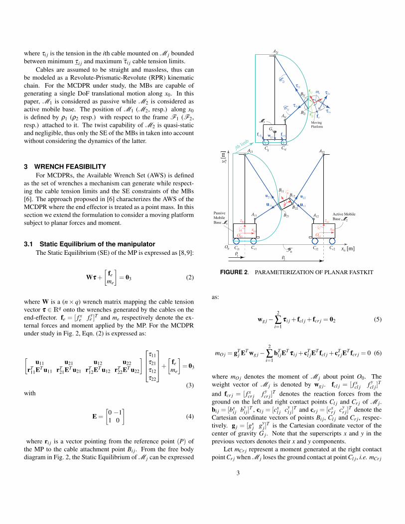
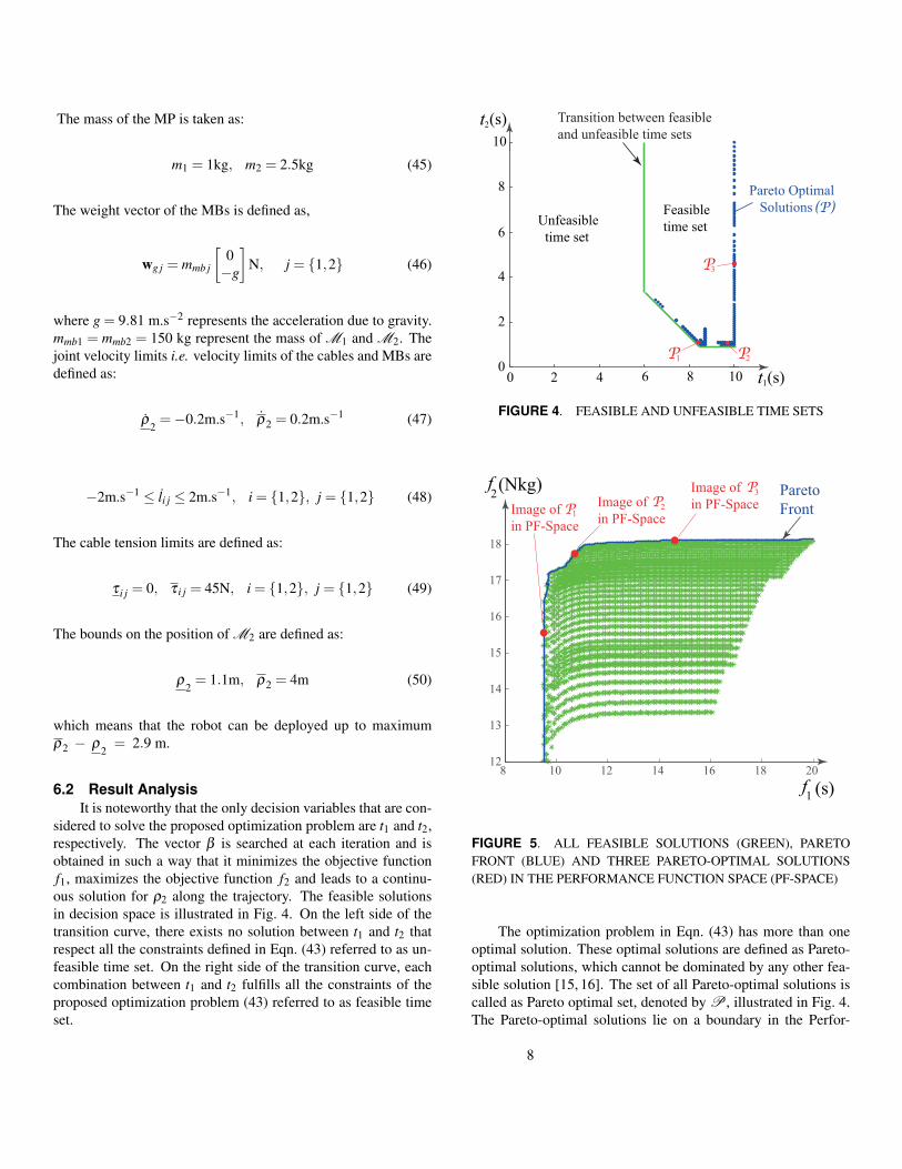
sidered to solve the proposed optimization problem are t1 and t2,respectively. The vector β is searched at each iteration and isobtained in such a way that it minimizes the objective functionf1, maximizes the objective function f2 and leads to a continu-ous solution for ρ2 along the trajectory. The feasible solutionsin decision space is illustrated in Fig. 4. On the left side of thetransition curve, there exists no solution between t1 and t2 thatrespect all the constraints defined in Eqn. (43) referred to as un-feasible time set. On the right side of the transition curve, eachcombination between t1 and t2 fulfills all the constraints of theproposed optimization problem (43) referred to as feasible timeset.
100
2
4
6
8
10
4 8620
1 P2
P3
P
(P)Unfeasible
time set
Feasible
time set
Pareto Optimal
Solutions
t (s)1
2Transition between feasible
and unfeasible time setst (s)
FIGURE 4. FEASIBLE AND UNFEASIBLE TIME SETS
8 10 12 14 16 18 2012
13
14
15
16
17
18
f1
f2 Pareto
Front
3PImage of
in PF-Space2PImage of
in PF-Space1PImage of
in PF-Space
(s)
(Nkg)
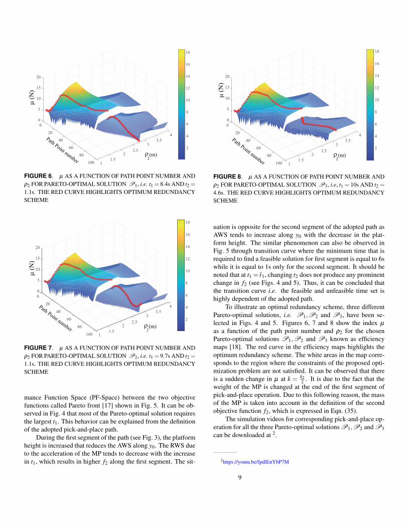
FIGURE 5. ALL FEASIBLE SOLUTIONS (GREEN), PARETOFRONT (BLUE) AND THREE PARETO-OPTIMAL SOLUTIONS(RED) IN THE PERFORMANCE FUNCTION SPACE (PF-SPACE)
The optimization problem in Eqn. (43) has more than oneoptimal solution. These optimal solutions are defined as Pareto-optimal solutions, which cannot be dominated by any other fea-sible solution [15, 16]. The set of all Pareto-optimal solutions iscalled as Pareto optimal set, denoted by P , illustrated in Fig. 4.The Pareto-optimal solutions lie on a boundary in the Perfor-
8
0
0
204
5
403
60
10
280
15
100 1
20
2
4
6
8
10
12
14
16
18
ρ 21.5
2.5
3.5
(m)
Path Point number
µ (
Ν)
FIGURE 6. µ AS A FUNCTION OF PATH POINT NUMBER ANDρ2 FOR PARETO-OPTIMAL SOLUTION P1, i.e. t1 = 8.4s AND t2 =1.1s. THE RED CURVE HIGHLIGHTS OPTIMUM REDUNDANCYSCHEME
0
0
204
5
403
60
10
280
15
100 1
20
2
4
6
8
10
12
14
16
18
ρ 21.5
2.5
3.5
(m)
Path Point number
µ (
Ν)
FIGURE 7. µ AS A FUNCTION OF PATH POINT NUMBER ANDρ2 FOR PARETO-OPTIMAL SOLUTION P2, i.e. t1 = 9.7s AND t2 =1.1s. THE RED CURVE HIGHLIGHTS OPTIMUM REDUNDANCYSCHEME
mance Function Space (PF-Space) between the two objectivefunctions called Pareto front [17] shown in Fig. 5. It can be ob-served in Fig. 4 that most of the Pareto-optimal solution requiresthe largest t1. This behavior can be explained from the definitionof the adopted pick-and-place path.
During the first segment of the path (see Fig. 3), the platformheight is increased that reduces the AWS along y0. The RWS dueto the acceleration of the MP tends to decrease with the increasein t1, which results in higher f2 along the first segment. The sit-
0
0
204
5
40Path Point number
360
10
280
15
100 1
20
2
4
6
8
10
12
14
16
18
ρ 21.5
2.5
3.5
(m)
µ (
Ν)
FIGURE 8. µ AS A FUNCTION OF PATH POINT NUMBER ANDρ2 FOR PARETO-OPTIMAL SOLUTION P3, i.e, t1 = 10s AND t2 =4.6s. THE RED CURVE HIGHLIGHTS OPTIMUM REDUNDANCYSCHEME
uation is opposite for the second segment of the adopted path asAWS tends to increase along y0 with the decrease in the plat-form height. The similar phenomenon can also be observed inFig. 5 through transition curve where the minimum time that isrequired to find a feasible solution for first segment is equal to 6swhile it is equal to 1s only for the second segment. It should benoted that at t1 = t1, changing t2 does not produce any prominentchange in f2 (see Figs. 4 and 5). Thus, it can be concluded thatthe transition curve i.e. the feasible and unfeasible time set ishighly dependent of the adopted path.
To illustrate an optimal redundancy scheme, three differentPareto-optimal solutions, i.e. P1,P2 and P3, have been se-lected in Figs. 4 and 5. Figures 6, 7 and 8 show the index µ
as a function of the path point number and ρ2 for the chosenPareto-optimal solutions P1,P2 and P3 known as efficiencymaps [18]. The red curve in the efficiency maps highlights theoptimum redundancy scheme. The white areas in the map corre-sponds to the region where the constraints of the proposed opti-mization problem are not satisfied. It can be observed that thereis a sudden change in µ at k = k2
2 . It is due to the fact that theweight of the MP is changed at the end of the first segment ofpick-and-place operation. Due to this following reason, the massof the MP is taken into account in the definition of the secondobjective function f2, which is expressed in Eqn. (35).
The simulation videos for corresponding pick-and-place op-eration for all the three Pareto-optimal solutions P1,P2 and P3can be downloaded at 2.
2https://youtu.be/fpdlEnYbP7M
9

7 CONCLUSIONIn this paper, a methodology to determine the optimal kine-
matic redundancy scheme of Planar Mobile Cable Driven Par-allel Robots (PMCDPRs) with one degree of kinematic redun-dancy for fast pick-and-place operations is described. First, theStatic equilibrium (SE) constraints of PMCDPRs associated withthe Mobile Bases (MBs) are formulated that are required to fullycharacterize the Available Wrench Set (AWS) of the latter. Then,a bi-objective optimization problem that corresponds to mini-mization of the total trajectory time and maximization of therobot average robustness index throughout the trajectory is for-mulated in order to determine the optimum kinematic redun-dancy scheme. A case study of a PMCDPR composed of twoMBs, four cables and a three degree-of-freedom (DoF) movingplatform is considered. Future work will deal with the experi-mental validation and the extension of the proposed methodol-ogy to spatial Mobile Cable Driven Parallel Robots (MCDPRs)with higher degrees of kinematic redundancy.
ACKNOWLEDGMENTThis research work is part of the European Project
ECHORD++ “FASTKIT” dealing with the development of col-laborative and Mobile Cable-Driven Parallel Robots for logistics.Ecole Centrale Nantes is also dutifully acknowledged for the fi-nancial support provided to the first author of the paper.
REFERENCES[1] Kawamura, S., Kino, H., and Won, C., 2000. “High-speed
manipulation by using parallel wire-driven robots”. Robot-ica, 18(1), pp. 13–21.
[2] Albus, J., Bostelman, R., and Dagalakis, N., 1993. “Thenist robocrane”. Journal of Field Robotics, 10(5), pp. 709–724.
[3] Lambert, C., Nahon, M., and Chalmers, D., 2007. “Imple-mentation of an aerostat positioning system with cable con-trol”. IEEE/ASME Transactions on Mechatronics, 12(1),pp. 32–40.
[4] Gagliardini, L., Caro, S., Gouttefarde, M., and Girin, A.,2016. “Discrete reconfiguration planning for cable-drivenparallel robots”. Mechanism and Machine Theory, 100,pp. 313–337.
[5] Rasheed, T., Long, P., Marquez-Gamez, D., and Caro, S.,2018. “Tension distribution algorithm for planar mobilecable-driven parallel robots”. In Cable-Driven ParallelRobots. Springer, pp. 268–279.
[6] Rasheed, T., Long, P., Gamez, D. M., and Caro, S.“Available wrench set for planar mobile cable-driven par-allel robots”. In 2018 IEEE International Conference onRobotics and Automation (ICRA).
[7] Rasheed, T., Long, P., Gamez, D. M., and Caro, S. “Kine-matic modeling and twist feasibility of mobile cable-drivenparallel robots”. In Advances in Robot Kinematics 2018.
[8] Kawamura, S., and Ito, K., 1993. “A new type of masterrobot for teleoperation using a radial wire drive system”.In Proceedings IEEE/RSJ Intelligent Robots and System(IROS) 1993, Vol. 1, IEEE, pp. 55–60.
[9] Hiller, M., Fang, S., Mielczarek, S., Verhoeven, R., andFranitza, D. “Design, analysis and realization of tendon-based parallel manipulators”. Mechanism and MachineTheory, 40(4), pp. 429–445, 2005.
[10] Gouttefarde, M., and Krut, S., 2010. “Characterization ofparallel manipulator available wrench set facets”. In Ad-vances in robot kinematics: motion in man and machine.Springer, pp. 475–482.
[11] Bouchard, S., Gosselin, C., and Moore, B., 2010. “On theability of a cable-driven robot to generate a prescribed setof wrenches”. Journal of Mechanisms and Robotics, 2(1),p. 011010.
[12] Guay, F., Cardou, P., Cruz-Ruiz, A. L., and Caro, S., 2014.“Measuring how well a structure supports varying externalwrenches”. In New Advances in Mechanisms, Transmis-sions and Applications. Springer, pp. 385–392.
[13] Ruiz, A. L. C., Caro, S., Cardou, P., and Guay, F., 2015.“Arachnis: Analysis of robots actuated by cables withhandy and neat interface software”. In Cable-Driven Par-allel Robots. Springer, pp. 293–305.
[14] Roberts, R. G., Graham, T., and Lippitt, T., 1998. “Onthe inverse kinematics, statics, and fault tolerance of cable-suspended robots”. Journal of Field Robotics, 15(10),pp. 581–597.
[15] Bui, L. T., Abbass, H. A., Barlow, M., and Bender, A.,2012. “Robustness against the decision-maker’s attitude torisk in problems with conflicting objectives”. IEEE Trans-actions on Evolutionary Computation, 16(1), pp. 1–19.
[16] Li, X., and Wong, H.-S., 2009. “Logic optimality for multi-objective optimization”. Applied Mathematics and Compu-tation, 215(8), pp. 3045–3056.
[17] Wang, W., Caro, S., Bennis, F., Soto, R., and Crawford,B., 2015. “Multi-objective robust optimization using apostoptimality sensitivity analysis technique: applicationto a wind turbine design”. Journal of Mechanical Design,137(1), p. 011403.
[18] Caro, S., Garnier, S., Furet, B., Klimchik, A., and Pashke-vich, A., 2014. “Workpiece placement optimization for ma-chining operations with industrial robots”. In Advanced In-telligent Mechatronics (AIM), 2014, IEEE, pp. 1716–1721.
10