Embed Size (px)
Citation preview
Working Paper No. 2014-6
May 2014
Optimal Joint Management of Interdependent Resources:
Groundwater vs. Kiawe (Prosopis pallida)
by
Kimerbly M. Burnett, James A. Roumasset and Christopher A. Wada
UNIVERSITY OF HAWAI‘ I AT MANOA
2424 MAILE WAY, ROOM 540 • HONOLULU, HAWAI‘ I 96822
WWW.UHERO.HAWAII .EDU
WORKING PAPERS ARE PRELIMINARY MATERIALS CIRCULATED TO STIMULATE
DISCUSSION AND CRITICAL COMMENT. THE VIEWS EXPRESSED ARE THOSE OF
THE INDIVIDUAL AUTHORS.
Optimal Joint Management of Interdependent Resources: Groundwater vs. Kiawe (Prosopis pallida)
Kimberly M. Burnett
University of Hawai‘i Economic Research Organization 2424 Maile Way, Saunders 540, Honolulu, HI 96822, USA
Tel.: +1 (808) 358-4126, Email: [email protected]
James A. Roumasset Department of Economics, University of Hawai‘i at Mānoa 2424 Maile Way, Saunders 542, Honolulu, HI 96822, USA
Tel.: +1 (808) 358-4126, Email: [email protected]
Christopher A. Wada
University of Hawai‘i Economic Research Organization 2424 Maile Way, Saunders 540, Honolulu, HI 96822, USA
Tel.: +1 (808) 358-4126, Email: [email protected]
ABSTRACT
Local and global changes continue to influence interactions between groundwater and terrestrial ecosystems. Changes in precipitation, surface water, and land cover can affect the water balance of a given watershed, and thus affect both the quantity and quality of freshwater entering the ground. Groundwater management frameworks often abstract from such interactions. However, in some cases, management instruments can be designed to target simultaneously both groundwater and an interdependent resource such as the invasive kiawe tree (Prosopis pallida), which has been shown to reduce groundwater levels. Results from a groundwater-kiawe management model suggest that at the optimum, the resource manager should be indifferent between conserving a unit of groundwater via tree removal or via reduced consumption. The model’s application to the Kona Coast (Hawai‘i) showed that kiawe management can generate a large net present value for groundwater users. Additional data will be needed to implement full optimization in the resource system.
Keywords: groundwater, kiawe, Prosopis pallida, renewable resources, resource management, dynamic optimization
1. INTRODUCTION
It is common in resource economics to solve for optimal harvest rates of an implicitly
independent resource (e.g., a forest stand, fishery, groundwater aquifer, or oil reserve). Yet, the
premise of ecological economics is that resources are interdependent. The objective of this
chapter is to help extend the principles of resource economics to deal with the joint management
of interdependent resources. It particularly considers the case where the groundwater uptake of
an invasive species detracts from the aquifer stock.
The standard economics approach of maximizing the present value (PV) of net benefits
generated by a natural resource specifies the optimal steady state stock level and characterizes
the path of optimal resource extraction leading up to that steady state. Decision rules for the
dynamically efficient (PV-maximizing) allocation of groundwater were first developed almost
half a century ago (Burt, 1967; Brown and Deacon, 1972). More recent efforts have refined the
hydrogeological aspects of the management framework, developed instruments for implementing
optimal extraction, and considered the welfare implications of various management strategies
(Gisser and Sánchez, 1980; Feinerman and Knapp, 1983; Moncur and Pollock, 1988; Tsur and
Zemel, 1995; Krulce et al., 1997; Brozović et al., 2010). Few, however, have considered the
simultaneous management of natural resources that are interconnected with the aquifer of
interest. Those that have modeled resource interdependency (both within and outside the
groundwater literature) typically focused on management of a single resource, taking harvest
from the adjacent resource as exogenous, e.g., shrimp farms and offshore fisheries (Barbier et al.,
2002), and groundwater and nearshore species such as seaweed (Duarte et al., 2010). In the
model presented herein, management decisions consider tradeoffs both between resources
(groundwater and kiawe) and over time.
Throughout Hawai‘i, kiawe (Prosopis pallida), a non-native tree introduced to the islands
in the early 19th century, can be found in both coastal wetlands and upland ecosystems, covering
58,766 ha or 3.55 percent of the state’s total land area A nitrogen-fixing legume. kiawe can
potentially reduce groundwater quality by providing nitrogen-rich organic material for leaching,
as well as reduce regional groundwater levels via deep taproots (Richmond and Mueller-
Dombois, 1972). In an application to the Kona Coast on the island of Hawai‘i, a basic
groundwater management model was modified to include water uptake by kiawe. When kiawe is
removed, groundwater extraction is higher in every period, corresponding to a lower water
scarcity value. In addition, the need for an alternative backstop resource such as desalinated
brackish water to meet growing demand is delayed. Both factors contribute to higher welfare in
present value terms. Present value gains from kiawe management were compared with present
value costs of removing and maintaining kiawe using several different methods. The net present
value is positive for each method, ranging from USD 17.0 million to 31.8 million.
2. GROUNDWATER-KIAWE MANAGEMENT FRAMEWORK
Although kiawe can affect nearshore ecosystems via increased nutrient loads, the study focused
only on its ability to reduce regional groundwater levels. A single-cell coastal aquifer model was
modified to include groundwater uptake by kiawe and was integrated into a management
framework, the objective of which is to maximize the present value of net benefits from water
consumption.
2.1. Groundwater Dynamics
Given that the study is interested in the long-run aquifer-level implications of management
decisions (i.e. it abstracts from spatial externalities associated with short-term pumping decisions
such as cones of depression), a single-cell aquifer model is used to determine changes in
groundwater stock over time. Under certain conditions (detailed in section 3), the stored volume
of water in a coastal aquifer is approximately related to the head level (h) – the distance between
mean sea level and the water table – by a constant factor of proportionality (γ). Recharge from
precipitation or adjacent water bodies (R) is assumed constant and exogenous. Stock-dependent
natural leakage along the freshwater-saltwater interface (L) is an increasing and convex function
of the head level; a high head level implies a larger groundwater lens, which exerts greater
pressure along a larger surface area. The quantity of groundwater extracted (q) is determined by
the resource manager in every period, and uptake (U) is an increasing function of the kiawe stock
(K). In what follows, a dot over a variable indicates its derivative with respect to time. The head
level evolves over time according the following relationship:
(1) γ ht = R− L(ht )− qt −U(Kt ).
2.2. Kiawe Dynamics
Kiawe provides some stock (e.g., pollen for the honey production industry) and extraction (e.g.,
charcoal) benefits to users in the region. However, the study views such benefits as small enough
relative to the potential value of water salvage from which they can be abstracted. In the more
general case where the benefits provided by both resources are substantial, the model can be
easily adjusted to include those benefits in the objective functional. The stock of kiawe increases
according to its natural net growth function (F) and decreases with anthropogenic removal (r):
(2) .)( ttt rKFK −=
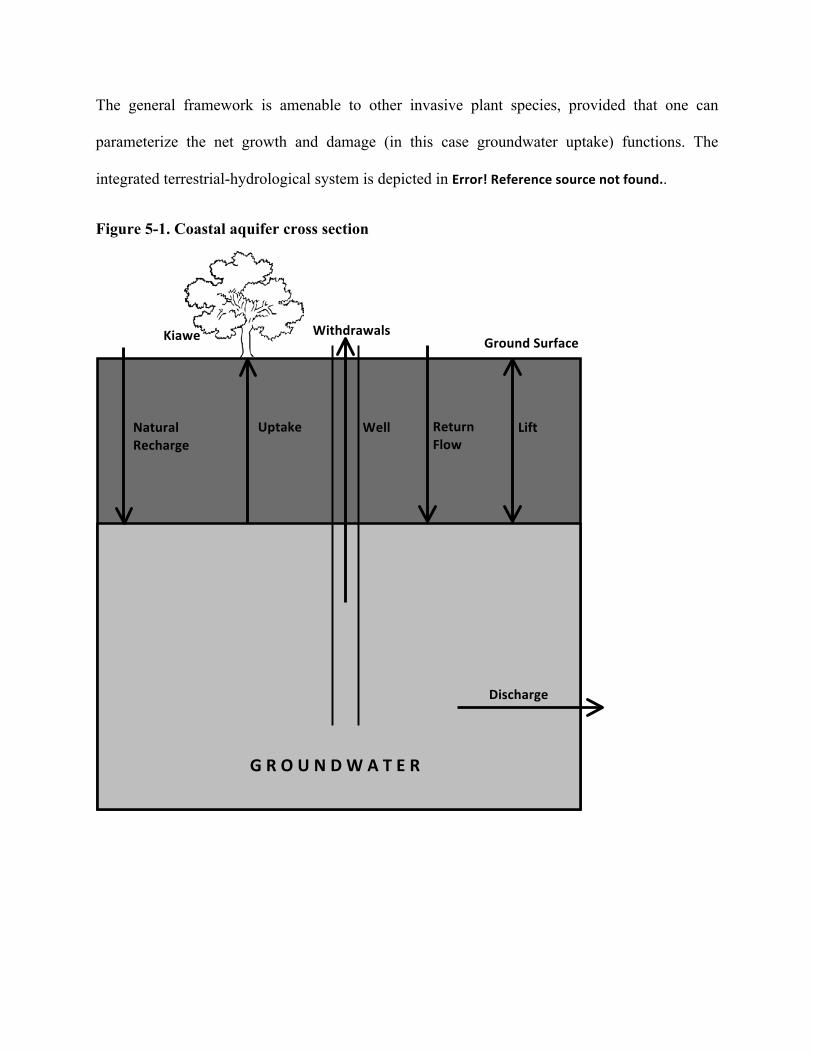
The general framework is amenable to other invasive plant species, provided that one can
parameterize the net growth and damage (in this case groundwater uptake) functions. The
integrated terrestrial-hydrological system is depicted in Error! Reference source not found..
Figure 5-1. Coastal aquifer cross section
Natural Recharge
Well
Withdrawals
Return Flow
Lift
Ground Surface
G R O U N D W A T E R
Discharge
Kiawe
Uptake
2.3. Present Value Maximization
The resource manager's problem is to choose the rates of groundwater extraction (q),
desalination (b), and kiawe removal (r) in every period to maximize the net present value (NPV),
that is:
(3) [ ]∫∞
=
− −−−+0
,,)()(),(max
tttrtbttqtt
t
rbqdtrKcbcqhctbqBe
ttt
ρ
subject to Eq. 1 and 2, given a positive discount rate ρ. Benefits (B) are a function of water
consumption (e.g., the area under the inverse demand curve). The unit extraction cost of
groundwater, cq(h), is a function of the head level because it is determined primarily by the
energy required to lift groundwater to the surface; as the water table declines, the distance
groundwater must be lifted increases. The cost of kiawe removal cr(K) is also stock-dependent
because management would entail targeting the lowest cost (e.g., the most accessible) areas first.
Desalinated water serves as a costly backstop resource, which can be used to supplement
groundwater at a constant unit cost cb.
If the price for which the marginal benefit and marginal cost of water extraction are equal
is defined as ),( tbqBp ttt +ʹ′≡ , then it is straightforward to construct the following efficiency
price equation for water (see Appendix I for a detailed derivation):
(4) [ ]
.)(
)()()()( 1
1
t
tttqttqt hL
KUhLRhcphcp
ʹ′+
−−ʹ′−+=
−
−
γρ
γ
The second term on the right hand side of Eq. 4 is the marginal user cost (MUC), or the loss in
present value resulting from an incremental reduction of the groundwater stock in period t. It is
identical to the usual MUC associated with groundwater extraction, except that the net recharge
term is adjusted by natural leakage and natural groundwater uptake from kiawe. All else equal,
the larger the uptake term, the larger is the MUC. Intuitively, this is because uptake adds to
anthropogenic extraction in drawing down the head level, thus creating higher future extraction
costs and hence larger PV losses than would be realized in the absence of kiawe.
An optimal management rule can also be constructed for the stock of kiawe (see Appendix I for a
detailed derivation):
(5) .)(
)()()]()[(1
t
trtttrt KU
KcKFKFKcʹ′
ʹ′−ʹ′−=− ρ
λγ
Kiawe should be removed until its marginal benefit in terms of avoided uptake, i.e., the shadow
value of water (γ-1λ), is equal to its marginal cost. The numerator of the cost term accounts for
the forgone interest that would have accrued had the income not been spent on tree removal, as
well as the effect on future kiawe growth and removal costs. Removing a tree today means that
future removal of the remaining trees is more expensive on a per-unit basis. It also means that the
rate of future kiawe growth is higher or lower, depending on where the stock resides on the
growth curve (F). The denominator converts the units of the numerator from dollars per tree to
dollars per unit of water. At the optimum, the manager should be indifferent between conserving
water via tree removal and via consumption reduction.
2.4. The Optimal Steady State
The optimality conditions (Eq. 4 and 5) must hold in every period, even when the system is in a
long-run equilibrium or steady state. By definition, the costate and state variables remain
constant in a steady state, i.e., 0==== tttt Kh µλ , which implies that 0=tp . If demand for
water grows over time as a result of rising per capita income and population expansion,
desalination will be eventually required at a finite time T to supplement groundwater
withdrawals. For bT cp = , Eq. 4 and 5 can be solved for unique values of head and kiawe stock,
hss and Kss, respectively. If the solution yields a negative value for Kss and/or hss < hmin, however,
one must instead conclude that Kss = 0 (i.e., eradication) and hss = hmin, where hmin is a minimum
allowable head level beyond which further pumping yields water of unacceptable quality.
The terminal conditions for head and kiawe stock can then be used in conjunction with initial
field measurements for h0 and K0 to numerically solve the system of equations (Eq. 1-2, 4-5).
Intuitively, any set of paths that satisfies Eq. 1 and 2 is feasible, but optimality requires that the
state variables also satisfy Eq. 4 and 5 in every period. Solving the problem thus involves
selecting the endogenous terminal time T such that the resulting paths are feasible, optimal, and
consistent with the initial conditions.
3. AN APPLICATION TO THE KONA COAST OF HAWAI‘I
A simplified version of the model presented in section 2 was applied to data from the Kiholo
aquifer and its surrounding watershed on the Kona Coast of Hawai‘i Island. The main departure
from the general framework is the absence of kiawe stock dynamics (Eq. 2). Although the
simplification rules out the possibility of dynamic tree management, the results still illustrate the
tradeoff between the recharge benefits and costs of kiawe removal.
3.1. Hydrology
The Kiholo aquifer is a thin basal or Ghyben-Herzberg lens of freshwater floating on underlying
denser seawater. Given the high porosity of the aquifer and hence its relatively thin brackish
transition zone (Duarte, 2002), the freshwater-saltwater mixing region was modeled as a sharp
interface. Although not amenable to characterizing spatial disequilibrium relationships in the
short-run, a one-dimensional aquifer model is still useful for identifying the long-run optimal
extraction path. The equation of motion for the head level of a one-dimensional, sharp-interface,
coastal aquifer can be expressed as ])()[41/2000( ttt qhLRWEh −−= θ , where θ is porosity, W
is the aquifer width, and E is the aquifer length (Mink, 1980). For the values θ=0.3, W=6000
meters, and E=6850 meters, the volume (thousand gallons) to head (feet) conversion factor (γ-1)
for the Kiholo aquifer is 0.0000000492.
Following Pongkijvorasin et al. (2010), the aquifer’s natural recharge is assumed constant
and equal to 3,992,700 thousand gallons per year (tg/yr). However, leakage or discharge from the
aquifer, as discussed previously, is not constant. Mink (1980) derived a structural expression for
discharge as a function of head: l(h)=kh2, where k is an aquifer-specific coefficient. Since the
leakage function needs to satisfy current conditions, a discharge rate of 3,883,330 tg/yr and head
level (h0) of 5.74 feet imply that k is equal to 117,864.
3.2. Groundwater Extraction and Desalination Costs
The cost of extracting groundwater is primarily determined by the energy required to lift water
from the subsurface aquifer to the ground level (e). Duarte (2002) estimated the energy cost of
lifting groundwater from the Kiholo aquifer to be USD (2001) 0.00083/m3 per meter. In 2012
dollars, the cost is USD 0.00108/m3 per m or equivalently USD 0.00125/tg/ft. Given that the
average ground elevation relative to mean sea level is 1,322.5 feet, the unit cost of groundwater
extraction as a function of the head level can be expressed as cq(h)=0.00125(1322.5-h).
Pitafi and Roumasset (2009) used a straightforward amortization procedure for capital costs
(e.g., treatment facility construction) in combination with cost projections for annual operation
and maintenance (e.g., wages, materials, energy) of a reverse osmosis desalination plant to
estimate the unit cost of desalination: USD (2001) 7/tg. After adjusting for inflation, cb was
estimated to be USD (2012) 9.07/tg.
3.3. Demand for Water
The County of Hawai‘i Department of Water Supply charges a fixed “standby charge,” a
volumetric “power cost charge,” and a volumetric “general use” rate that varies discretely by
water quantity blocks. Assuming that the average family falls into the second price block—
which is consistent with the average household use of roughly 13,000 gallons per month on
O‘ahu—the retail price for water in the region was USD (2008) 4.80/tg.
At the price of USD 4.80/tg, 1074.4 m3 of groundwater were extracted for consumption
in 2008. Based on Griffin (2006) and Dalhuisen et al. (2003), the price elasticity of demand for
water (η) is assumed at -0.7, which corresponds to a constant elasticity demand function of the
form qt=850983pt-0.7, measured in tg/yr. With the development of projects in the area, extraction
is expected to increase to 3809 m3/yr (Pongkijvorasin, 2007). A 5 percent growth rate of demand
is consistent with a 25-year period to project completion and similar growth thereafter. However,
a more reasonable assumption may be that in the years following completion of the projects,
population and per capita income growth would converge to a lower level. Therefore, it is
assumed that demand grows at an average rate of 3 percent per annum, such that period t demand
is determined by qt=850983pt-0.7e0.03t.
3.4. Groundwater Uptake by Kiawe
Ideally, a relationship between kiawe and water uptake could be constructed using a time series
of relevant data. In the absence of the requisite data, however, potential water salvage of kiawe
removal can be roughly estimated using such a relationship for a similar type of tree. Saltcedar
(Tamarix spp.), for example, is also known to lower water tables via deep taproots, particularly
in the southwestern United States. Barz et al. (2009) estimated that removal of 8,954 acres of
saltcedar from the Texas Pecos River Basin would release 7.41 million m3 of water per year.
This translates to an annual recharge gain of 218.62 tg of water per acre of trees removed.
Assuming that kiawe is roughly distributed in proportion to land area for each of the
islands across the state and that one-fourth of the kiawe habitat on Hawai‘i Island lies on the
Kona Coast in close proximity to the Kiholo aquifer, the total potential water salvage associated
with removing all of the kiawe in Kiholo is 2,936,570 tg/yr. These along with the other functions
and parameters discussed in sections 3.1-3.3 are summarized in Error! Reference source not
found..
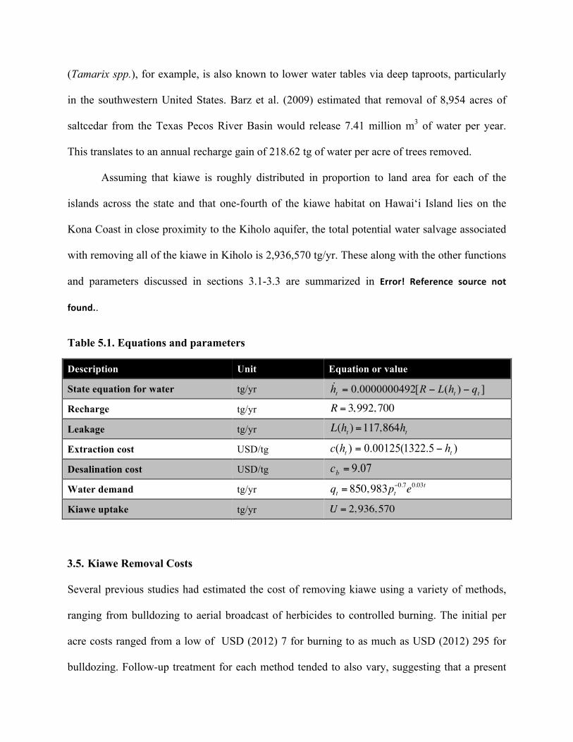
Table 5.1. Equations and parameters
Description Unit Equation or value
State equation for water tg/yr ])([0000000492.0 ttt qhLRh −−=
Recharge tg/yr R = 3,992, 700
Leakage tg/yr L(ht ) =117,864ht
Extraction cost USD/tg )5.1322(00125.0)( tt hhc −=
Desalination cost USD/tg 07.9=bc
Water demand tg/yr qt = 850,983pt−0.7e0.03t
Kiawe uptake tg/yr U = 2,936,570
3.5. Kiawe Removal Costs
Several previous studies had estimated the cost of removing kiawe using a variety of methods,
ranging from bulldozing to aerial broadcast of herbicides to controlled burning. The initial per
acre costs ranged from a low of USD (2012) 7 for burning to as much as USD (2012) 295 for
bulldozing. Follow-up treatment for each method tended to also vary, suggesting that a present
value approach to calculating costs is necessary to ensure that streams of costs accruing in
different time periods are converted to comparable units. Thus for an initial treatment cost of $X
followed by maintenance treatment every Y years at a cost of $Z, the PV cost of removal is
calculated as ])1([$$1∑
∞
=
−++t
YtZX ρ per acre. Per acre costs and PV costs for removing all
existing acres of kiawe in the Kiholo region are presented in Error! Reference source not found..
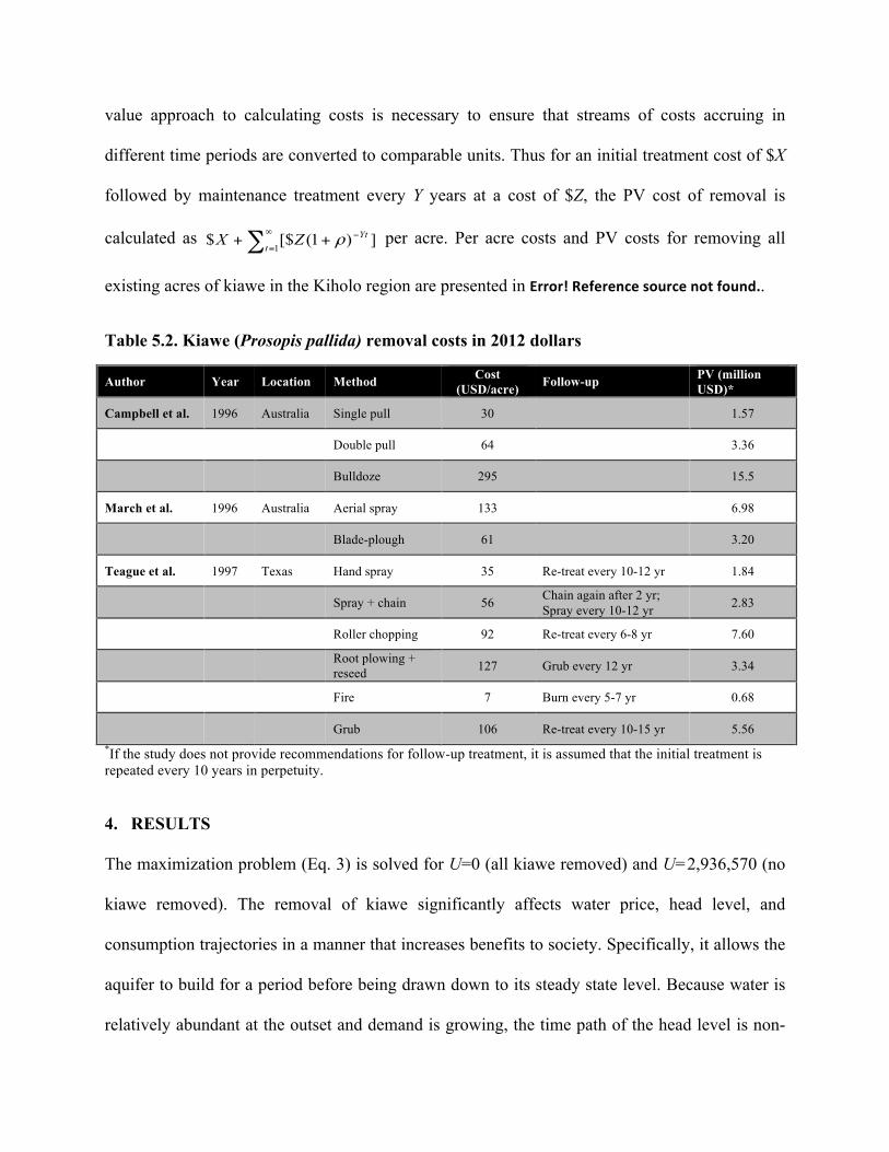
Table 5.2. Kiawe (Prosopis pallida) removal costs in 2012 dollars
Author Year Location Method Cost (USD/acre) Follow-up PV (million
USD)*
Campbell et al. 1996 Australia Single pull 30 1.57
Double pull 64 3.36
Bulldoze 295 15.5
March et al. 1996 Australia Aerial spray 133 6.98
Blade-plough 61 3.20
Teague et al. 1997 Texas Hand spray 35 Re-treat every 10-12 yr 1.84
Spray + chain 56 Chain again after 2 yr; Spray every 10-12 yr 2.83
Roller chopping 92 Re-treat every 6-8 yr 7.60
Root plowing + reseed 127 Grub every 12 yr 3.34
Fire 7 Burn every 5-7 yr 0.68
Grub 106 Re-treat every 10-15 yr 5.56 *If the study does not provide recommendations for follow-up treatment, it is assumed that the initial treatment is repeated every 10 years in perpetuity.
4. RESULTS
The maximization problem (Eq. 3) is solved for U=0 (all kiawe removed) and U=2,936,570 (no
kiawe removed). The removal of kiawe significantly affects water price, head level, and
consumption trajectories in a manner that increases benefits to society. Specifically, it allows the
aquifer to build for a period before being drawn down to its steady state level. Because water is
relatively abundant at the outset and demand is growing, the time path of the head level is non-
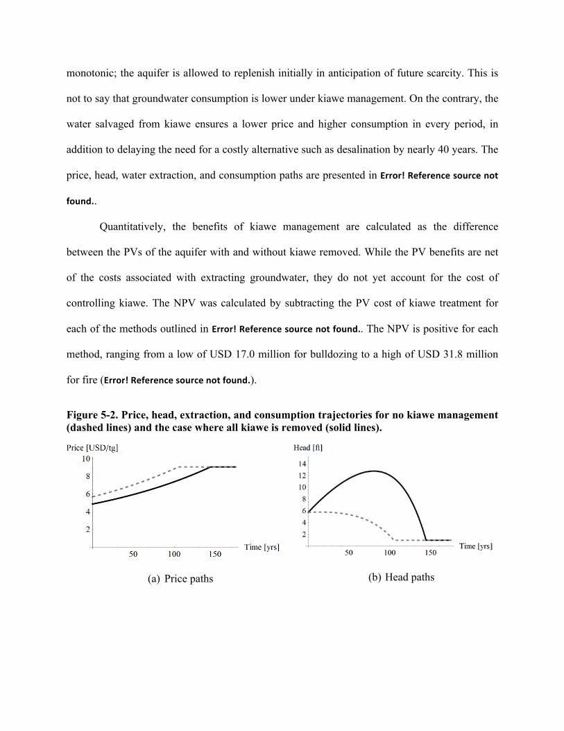
monotonic; the aquifer is allowed to replenish initially in anticipation of future scarcity. This is
not to say that groundwater consumption is lower under kiawe management. On the contrary, the
water salvaged from kiawe ensures a lower price and higher consumption in every period, in
addition to delaying the need for a costly alternative such as desalination by nearly 40 years. The
price, head, water extraction, and consumption paths are presented in Error! Reference source not
found..
Quantitatively, the benefits of kiawe management are calculated as the difference
between the PVs of the aquifer with and without kiawe removed. While the PV benefits are net
of the costs associated with extracting groundwater, they do not yet account for the cost of
controlling kiawe. The NPV was calculated by subtracting the PV cost of kiawe treatment for
each of the methods outlined in Error! Reference source not found.. The NPV is positive for each
method, ranging from a low of USD 17.0 million for bulldozing to a high of USD 31.8 million
for fire (Error! Reference source not found.).
Figure 5-2. Price, head, extraction, and consumption trajectories for no kiawe management (dashed lines) and the case where all kiawe is removed (solid lines).
(a) Price paths
(b) Head paths
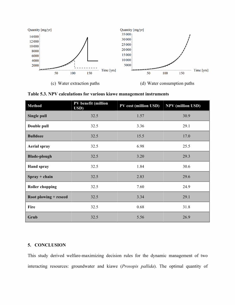
(c) Water extraction paths
(d) Water consumption paths
Table 5.3. NPV calculations for various kiawe management instruments
Method PV benefit (million USD) PV cost (million USD) NPV (million USD)
Single pull 32.5 1.57 30.9
Double pull 32.5 3.36 29.1
Bulldoze 32.5 15.5 17.0
Aerial spray 32.5 6.98 25.5
Blade-plough 32.5 3.20 29.3
Hand spray 32.5 1.84 30.6
Spray + chain 32.5 2.83 29.6
Roller chopping 32.5 7.60 24.9
Root plowing + reseed 32.5 3.34 29.1
Fire 32.5 0.68 31.8
Grub 32.5 5.56 26.9
5. CONCLUSION
This study derived welfare-maximizing decision rules for the dynamic management of two
interacting resources: groundwater and kiawe (Prosopis pallida). The optimal quantity of
groundwater extraction satisfies the condition that the marginal benefit of water consumption is
equal to the sum of extraction and marginal user cost, where the latter is a function not only of
the groundwater stock but also of the kiawe stock via its ability for groundwater uptake.
Analogously, the optimal decision rule for kiawe control is dependent on the stock of
groundwater; kiawe should be removed until the marginal benefit in terms of water salvage is
equal to the marginal cost of removal. At the optimum, which can be achieved only through joint
management of the resources, the costs of conserving water via tree removal and consumption
reduction are equal. One way of implementing the optimal solution is by setting the marginal
water price equal to the cost of providing water through both mechanisms.
An application of the model to the Kona Coast of Hawai‘i showed that the PV cost of
removing existing kiawe trees is outweighed by the benefits, measured as the difference in PV
welfare to water consumers with and without the trees removed. Among the 11 removal methods
considered, management by fire yields the lowest PV cost (USD 0.68 million) and hence the
highest net PV (USD 31.8 million), while management by bulldozing yields the highest PV cost
(USD 15.5 million) and the lowest net PV (USD 17.0 million). However, the NPV estimates
considered only the direct costs of management (e.g., wages, materials, equipment rental). Each
removal instrument may generate additional costs that must be accounted when devising a
management strategy. Fire, for example, does not require much labor or rental of expensive
machinery, but the potential for spread to non-targeted areas may not be trivial, especially in dry
leeward areas conducive to kiawe growth. The smoke generated might also cause discomfort to
surrounding residents. Herbicide application is effective, but has the potential to affect non-target
native species and to compromise the quality of underlying groundwater sources. Obtaining
permits for aerial broadcast of herbicides may be prohibitively costly or difficult. Thus, Error!
Reference source not found. should be a viewed as primarily a starting point for the development
of kiawe management policy.
Regardless of method, kiawe removal may disrupt other activities that generate benefits.
For instance, although it is an invasive species in Hawai‘i, kiawe is valued for its role in honey
production and as firewood. These industries are small relative to the state’s economy, but the
potential welfare loss should be incorporated into a comprehensive benefit-cost analysis of
various management instruments under consideration. While a detailed analysis of the impact on
the local economy is beyond the scope of this chapter, any losses suffered by those industries are
believed to likely be outweighed by the potential recharge benefits of management, inasmuch as
the kiawe under consideration in Kiholo composes only a fraction of the forest stands on the
island and in the state.
The framework developed herein can be applied to a variety of settings around the world,
where the presence of one natural stock affects the quantity, quality, or availability of another.
Other appropriate applications include jointly managing upstream forests and downstream
waterways, invasive pest control in agriculture, and groundwater management and linked
nearshore marine ecosystems. To the extent that the relationships between natural stocks, as well
as the implications of changing one or the other, can be characterized, optimal management
trajectories for maximizing their joint benefit can be obtained.
From a policy perspective, one can draw several lessons from the framework developed.
First, resource scarcity can be largely affected by interlinkages between different types of
ecosystems or natural resources, so management decisions such as price reform should consider
those interlinkages. Relatedly, managing resources independently – e.g., a groundwater aquifer
and an invasive species such as kiawe that affects the aquifer – overlooks potentially large
welfare gains that may be obtained from joint management. Lastly, even when currently
available data are not sufficient to jointly optimize both resources, management scenarios such as
removing all of the invasive species in the current period may serve as a useful approximation
(or lower bound) of NPV benefits to justify financing a joint management approach.
The analysis presented can be extended in a variety of ways. The NPV calculations
assume that kiawe reduction would occur immediately, when in fact it may make sense to delay
the removal of the trees. If the discount rate is large (future benefits and costs are not valued
highly from today’s standpoint) and groundwater is initially relatively abundant, consumers may
prefer to delay the cost of kiawe management. In that case, the problem becomes one of optimal
timing: at what point in the future should kiawe trees be removed to maximize PV? An even
more ambitious extension would involve determining the optimal dynamic path of kiawe
reduction, provided that data are available to parameterize detailed uptake and growth functions.
REFERENCES
Barbier, Edward B., Strand, Ivar, Sathirathai, Suthawan. (2002). “Do open access conditions
affect the valuation of an externality? Estimating the welfare effects of mangrove-fishery
linkages in Thailand”. Environmental and Resource Economics 21, 343-367.
Barz, Dave, Watson, Richard P., Kanney, Joseph F., Roberts, Jesse D., Groeneveld, David P.
(2009). “Cost/Benefit considerations for recent saltcedar control, Middle Pecos River,
New Mexico”. Environmental Management 43, 282-298.
Brown, Gardner, Deacon, Robert. (1972). “Economic optimization of a single cell aquifer”.
Water Resources Research 8, 552-564.
Brozović, Nicholas, Sunding, David L., Zilberman, David. (2010). “On the spatial nature of the
groundwater pumping externality”. Resource and Energy Economics 32, 154-164.
Burt, Oscar R. (1967). “Temporal allocation of groundwater”. Water Resources Research 3, 45-
56.
Campbell, S.D., Setter, C.L., Jeffrey, P.L., Vitelli, J. (1996). “Controlling dense infestations of
Prosopis pallida”. Proceedings of the 11th Australian Weeds Conference, Melbourne
Australia, 30 September – 3 October 1996.
Chiang, Alpha C. (2000). Elements of Dynamic Optimization. Waveland Press, Inc., Illinois.
Dalhuisen, Jasper M., Florax, Raymond J.G.M., de Groot, Henri L.F., Nijkamp, Peter. (2003).
“Price and income elasticities of residential water demand: a meta-analysis”. Land
Economics 79(2), 292–308.
Duarte, Thomas K. (2002). “Long-term management and discounting of groundwater resources
with a case study of Kuki’o, Hawaii”. Ph.D dissertation. Department of Civil and
Environmental Engineering, Massachusetts Institute of Technology.
Duarte, Thomas K., Pongkijvorasin, Sittidaj, Roumasset, James, Amato, Daniel, Burnett,
Kimberly. (2010). “Optimal management of a Hawaiian coastal aquifer with nearshore
marine ecological interactions”. Water Resources Research 46, W11545.
Feinerman, Eli, Knapp, Keith C. (1983). “Benefits from Groundwater Management: Magnitude,
Sensitivity, and Distribution”. American Journal of Agricultural Economics 65, 703-710.
Gisser, Micha, Sánchez, David A. (1980). “Competition versus optimal control in groundwater
pumping”. Water Resources Research 31, 638-642.
Griffin, Ronald C. (2006). Water Resource Economics: The Analysis of Scarcity, Policies and
Projects. The MIT Press, Cambridge, MA.
Krulce, Darrell L., Roumasset, James A., Wilson, Tom. (1997). “Optimal management of a
renewable and replaceable resource: the case of coastal groundwater”. American Journal
of Agricultural Economics 79, 1218-1228.
March, Nathan, Akers, David, Jeffrey, Peter, Vietlli, Joe, Mitchell, Trevor, James, Peter,
Mackey, A.P. (1996). “Mesquite (Prosopis spp.) in Queensland”. Pest Status Review
Series – Land Protection Branch. Department of Natural Resources and Mines,
Queensland, Australia.
Mink, John F. (1980). State of the Groundwater Resources of Southern Oahu. Board of Water
Supply, Honolulu.
Moncur, James E.T., Pollock, Richard L. (1988). “Scarcity rents for water: a valuation and
pricing model”. Land Economics 64(1), 62-72.
Pitafi, Basharat A., Roumasset, James A. (2009). “Pareto-improving water management over
space and time: the Honolulu case”. American Journal of Agricultural Economics 91(1),
138–153.
Pongkijvorasin, Sittidaj. (2007). “Stock-to-stock externalities and multiple resources in
renewable resource economics: watersheds, conjunctive water use, reefs and mud”. Ph.D.
dissertation. Department of Economics, University of Hawai‘i at Mānoa, Hawai’i.
Pongkijvorasin, Sittidaj, Roumasset, James, Duarte, Thomas K., Burnett, Kimberly. (2010).
“Renewable resource management with stock externalities: coastal aquifers and
submarine groundwater discharge”. Resource and Energy Economics 32, 277-291.
Richmond, T. de A., Mueller-Dombois, D. (1972). “Coastline ecosystems on Oahu, Hawaii”.
Plant Ecology 25, 367-400.
Teague, Richard, Borchardt, Rob, Ansley, Jim, Pinchak, Bill, Cox, Jerry, Foy, Joelyn K.,
McGrann, Jim. (1997). “Sustainable management strategies for mesquite rangeland: the
Waggoner Kit Project”. Rangelands 19(5), 4-8.

Tsur, Yacov, Zemel, Amos. (1995). “Uncertainty and irreversibility in groundwater resource
management”. Journal of Environmental Economics and Management 29, 149-161.

Acknowledgements
This research was funded in part by NSF EPSCoR Grant No. EPS-0903833.
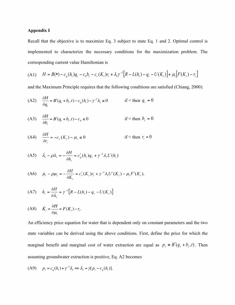
Appendix I
Recall that the objective is to maximize Eq. 3 subject to state Eq. 1 and 2. Optimal control is
implemented to characterize the necessary conditions for the maximization problem. The
corresponding current value Hamiltonian is
(A1) [ ] [ ]tttttttttrtbttq rKFKUqhLRrKcbcqhcBH −+−−−+−−−= − )()()()()()( 1 µγλ
and the Maximum Principle requires that the following conditions are satisfied (Chiang, 2000):
(A2) ∂H∂qt
= "B (qt + bt, t)− cq (ht )−γ−1λt ≤ 0
if < then 0=tq
(A3) ∂H∂bt
= "B (qt + bt, t)− cb ≤ 0 if < then 0=tb
(A4) 0)( ≤−−=∂
∂ttr
t
KcrH
µ if < then 0=tr
(A5) )()( 1ttttq
ttt hLqhc
hH
ʹ′+ʹ′=∂
∂−=− − λγρλλ
(A6) ).()()( 1ttttttr
ttt KFKUrKc
KH
ʹ′−ʹ′+ʹ′=∂
∂−=− − µλγρµµ
(A7) [ ])()(1ttt
tt KUqhLRHh −−−=
∂
∂= −γ
λ
(A8) Kt =
∂H∂µt
= F(Kt )− rt.
An efficiency price equation for water that is dependent only on constant parameters and the two
state variables can be derived using the above conditions. First, define the price for which the
marginal benefit and marginal cost of water extraction are equal as ),( tbqBp ttt +ʹ′≡ . Then
assuming groundwater extraction is positive, Eq. A2 becomes
(A9) pt = cq (ht )+γ−1λt ⇔ λt = γ[pt − cq (ht )].
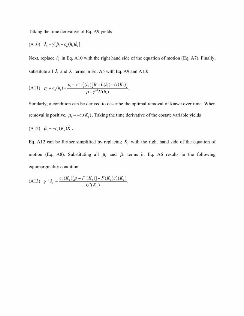
Taking the time derivative of Eq. A9 yields
(A10) λt = γ[ pt − "cq (ht ) ht ].
Next, replace ht in Eq. A10 with the right hand side of the equation of motion (Eq. A7). Finally,
substitute all λt and λt terms in Eq. A5 with Eq. A9 and A10:
(A11) pt = cq (ht )+pt −γ
−1 "cq (ht ) R− L(ht )−U(Kt )[ ]ρ +γ −1 "L (ht )
.
Similarly, a condition can be derived to describe the optimal removal of kiawe over time. When
removal is positive, µt = −cr (Kt ) . Taking the time derivative of the costate variable yields
(A12) µt = − "cr (Kt ) Kt.
Eq. A12 can be further simplified by replacing Kt with the right hand side of the equation of
motion (Eq. A8). Substituting all µt and µt terms in Eq. A6 results in the following
equimarginality condition:
(A13) .)(
)()()]()[(1
t
trtttrt KU
KcKFKFKcʹ′
ʹ′−ʹ′−=− ρ
λγ