Optimal design of storm water inlets for highway drainagejh.iwaponline.com/content/ppiwajhydro/6/4/245.full.pdf · Optimal design of storm water inlets for highway drainage ... evaluated

Optimal design of storm water inlets for highway

drainage

John W. Nicklow and Anders P. Hellman

John W. Nicklow (corresponding author)Department of Civil and Environmental

Engineering,Southern Illinois University Carbondale,Carbondale,IL 62901,USATel: +1 618 453 3325;Fax: +1 618 453 3044;E-mail: [email protected]

Anders P. HellmanGrundvattenteknik AB,Falun,Sweden

ABSTRACT

A new methodology and computational model are developed for direct evaluation of an optimal

storm water inlet design. The optimal design is defined as the least-cost combination of inlet types,

sizes and locations that effectively drain a length of pavement. Costs associated with inlets are

user-defined and can include those associated with materials, installation and maintenance, as well

as other project-related expenses. Effective drainage is defined here as maintaining a spatial

distribution of roadway spread, or top width of gutter flow, that is less than the allowable width of

spread. The solution methodology is based on the coupling of a genetic algorithm and a hydraulic

simulation model. The simulation model follows design guidelines established by the Federal

Highway Administration and is used to implicitly solve governing hydraulic constraints that yield

gutter discharge, inlet interception capacity and spread according to a design storm. The genetic

algorithm is used to select the best combination of design parameters and thus solves the overall

optimization problem. Capabilities of the model are successfully demonstrated through application

to a hypothetical, yet realistic, highway drainage system. The example reveals that genetic

algorithms and the optimal control methodology comprise a comprehensive decision-making

mechanism that can be used for cost-effective design of storm water inlets and may lead to a

reduced overall cost for highway drainage.

Key words | storm water, inlet design, optimal control, genetic algorithm

INTRODUCTION

Highways are designed to facilitate traffic movement at

specified service levels. The accumulation of water on

roadways, however, can pose a significant threat to traf-

fic safety and highway functionality by disrupting traffic

flow, increasing vehicular skid distance, raising the

potential for hydroplaning and accelerating pavement

deterioration (AASHTO 1991; Brown et al. 1996). (The

term pavement as used herein refers to an asphalt or

concrete roadway) As a result, design, installation and

maintenance of facilities to remove highway runoff com-

prise integral parts of the overall roadway design process

and can comprise more than 25% of total highway con-

struction costs (Mays 1979). The objective in designing

such drainage facilities is ultimately to collect runoff in

gutters and intercept flow at storm water inlets in a

manner that provides a high degree of traffic safety while

limiting costs.

There are two categories of design variables that deter-

mine the effectiveness of storm water inlets in intercepting

roadside gutter flow: (1) the type and size of inlets to be

utilized, and (2) the required number and corresponding

locations of inlets to be installed. The interactions

between these variables and the resulting gutter flow

characteristics are complicated. First, there are many

available sizes of each of the four major inlet types (grates,

curb-openings, slotted-drains and combination inlets).

Second, the same inlet may operate hydraulically as a weir

at shallow water depths and as an orifice when the inlet is

submerged. Finally, different gutter geometries and inlet

configurations will cause a wide variation in top width of

245 © IWA Publishing 2004 Journal of Hydroinformatics | 06.4 | 2004

gutter flow, or roadway spread. Fortunately, generalized

design procedures are well documented by many urban

drainage criteria and design manuals (Brown et al. 1996;

Johnson & Chang 1984; IDOT 1989). The real difficulty for

the designer, however, lies in finding the combination

of these design parameters that solves the following

optimization model:

Minimize→the material, installation, maintenance

and other costs associated with inlets used in design.

Subject To→(i) the physical laws that govern

pavement drainage, and (ii) bound constraints on

the spread of water onto the pavement.

According to a selected combination of design parameters,

the designer traditionally solves the governing equations

to evaluate the effectiveness of each inlet and the resulting

spatial distribution of spread. If the computed roadway

spread exceeds that which is allowable, typically estab-

lished by local, state or federal guidelines, an alternative

set of design parameters must be selected and the process

repeated. Consequently, determination of the most eco-

nomical design that effectively drains a section of highway

becomes an even more computationally intensive and

time-consuming, if not impossible, task. Using this

iterative, trial and error technique, every potential design

alternative would require evaluation before an optimum

could be declared. Furthermore, if one design appears

more costly than another, it is nearly impossible to

ascertain whether the difference in cost is merely due to

poor selection of design variables or due to real differences

in drainage effectiveness.

This paper discusses the development of the first opti-

mal control methodology for solving the storm water inlet

design problem. The optimal control approach that is

implemented is based on a computational interface

between hydraulic simulation and optimization tech-

niques. Applications of this interfacing methodology have

been increasingly popular in the fields of hydraulics and

hydrology and have provided solutions for complex prob-

lems in areas of reservoir management (Nicklow & Mays

2000; Unver & Mays 1990; Yeh 1985), bioremediation

design and groundwater management (Wanakule et al.

1986; Yeh 1992; Minsker & Shoemaker 1998) and the

design and operation of water distribution systems (Cunha

& Sousa 2000; Sakarya & Mays 2000). Nicklow (2000)

provides a comprehensive review of the benefits of this

approach, which include a reduced need for additional

simplifying assumptions about the physical system in

order to reach an optimal solution and a decrease in size

of the overall optimization problem. Such an approach,

however, has not been previously applied to solve the inlet

design problem. Elimam et al. (1989) evaluated the optimal

design of gravity sewer networks using linear program-

ming. Templeman & Walters (1979) and Li & Matthew

(1990) applied variations of dynamic programming to

determine the optimal geometric layout of subsurface

drainage networks, while Mays (1979) applied a similar

methodological approach for least-cost culvert design.

When applied to the inlet design problem, the meth-

odology is formulated to directly evaluate the least-cost

design that will effectively drain a roadway section, thus

overcoming limitations associated with trial-and-error

design approaches, and in turn leads to a reduced total

highway construction cost. Furthermore, by incorporating

standard hydraulic simulation procedures that have been

widely accepted in engineering practice, the optimal

control model attempts to integrate existing technologies

and improve the practical utility of the new methodology.

PROBLEM FORMULATION

For the storm water inlet problem, the matrix of decision

(design) variables is comprised of inlet types and sizes, as

well as the number of inlets required and their location.

The state (dependent) vector is the spatial variation of

spread along the pavement and the resulting cost of the

design. The problem can be expressed mathematically as

Min Z � ∑j � 1

J

njCj (1)

subject to

Ti + 1 = f(Ti,Ui) for 1%i%I − 1 (2)

0%Ti%Tmax (3)

246 J. W. Nicklow and A. P. Hellman | Optimal design of storm water inlets for highway drainage Journal of Hydroinformatics | 06.4 | 2004

j∈J* (4)

where Z is the total cost of inlets, nj is the number of inlets

of type j used in the design, Cj is the cost associated with

inlet type j, J is the number of different types, including

sizes, of inlets used in the design, Ti + 1 is the roadway

spread at discrete location i + 1, which depends on the

spread at the adjacent upstream location i, I is the total

number of discrete locations at which spread is evaluated,

Ui represents the design variables, if any, that are

implemented at section i, Tmax is the maximum

permissible spread, set as a design criterion and J*

represents the set of predefined inlet types and sizes that

are made available for a particular design application.

Equation (1) is the separable objective function to be

minimized and represents the total cost of inlets, which

can include material, installation (i.e. construction),

maintenance and other expenses. Although the current

formulation considers only user-defined, fixed unit costs,

they could easily be permitted to vary (i.e. volume dis-

counts based on the quantity of inlets or the number of

inlet types used). In addition, while other objectives are

possible for inlet design, such as minimizing the number

of required inlets or minimizing cumulative spread, the

function will implicitly depend on the current set of design

variables. Equation (2) is the transition, or simulation,

constraint that represents the governing hydraulic

relationship of highway drainage and describes system

behavior in response to the current design alternative. For

example, the spread of water at a particular location will

depend on the decision of whether to install an inlet

immediately upstream of that location, as well as the

decision regarding the type and size of inlet to be used.

Finally, Equations (3) and (4) are bound constraints used

to define a feasible range for roadway spread and inlets

selected for the design. The overall problem can therefore

be translated as the determination of the types, sizes and

locations of particular inlets that both minimize costs and

effectively drain the pavement at a level of spread that

does not exceed that which is allowable.

The inlet design problem formulation represents a

large-scale, nonlinear programming problem for which

there are no explicit solution schemes. The formula-

tion can be solved, however, by interfacing a hydraulic

simulation model with a genetic algorithm (GA). The

simulation model is used to implicitly solve the transition

constraint that yields gutter discharge, interception

capacity and spread according to design flow criteria.

Subsequently, the GA is used to select the best combina-

tion of design parameters to solve the overall optimization

problem.

HIGHWAY DRAINAGE SIMULATION

The simulation model developed for the optimal control

methodology was written specifically for this project

and is based upon design guidelines established by the

Federal Highway Administration (Brown et al. 1996) and

further explained by Nicklow (2001). While other, more

advanced and even more accurate, simulation methods

could be integrated to solve the inlet design problem, a

large majority of consultant designers and state agencies

commonly rely upon these guidelines in some form,

whether applied directly or integrated into a prepackaged

design model. The simulation model described herein is

specifically comprised of preprocessing and drainage com-

putation modules. The overall model handles all hydro-

logic and hydraulic computations and is capable of

evaluating the maximum spacing of a series of predefined

inlet types, without exceeding allowable spread criteria.

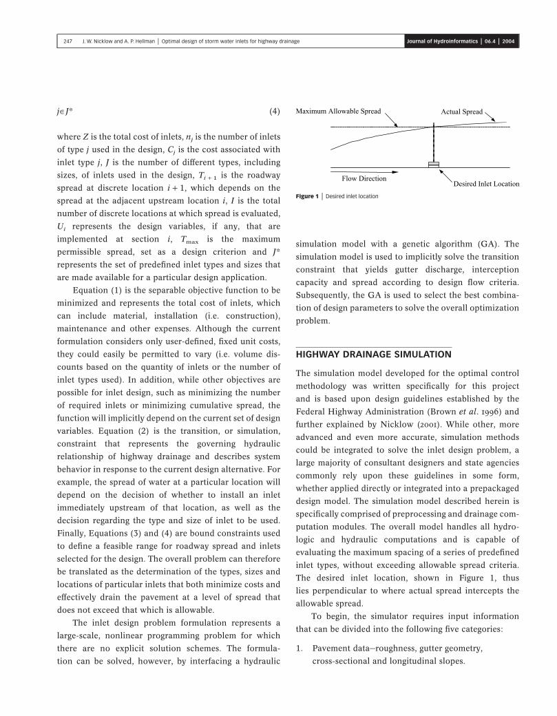
The desired inlet location, shown in Figure 1, thus

lies perpendicular to where actual spread intercepts the

allowable spread.

To begin, the simulator requires input information

that can be divided into the following five categories:

1. Pavement data—roughness, gutter geometry,

cross-sectional and longitudinal slopes.

Figure 1 | Desired inlet location


2. Rainfall data—discrete intensity–duration–frequency

(IDF) data for a design storm.

3. Longitudinal slope—slope at discrete positions along

the pavement.

4. Additional flow—additional offsite runoff added to

total gutter flow at discrete positions.

5. Inlet characteristics—type, size and placement order

of inlets.

The full length of the pavement considered is divided into

a number of evenly distributed shorter segments. Although

the length of individual segments can be user-defined, the

default length is one unit (e.g. 1 m). Data points, located

at the end of each segment, represent locations where flow

rate, spread and other hydraulic characteristics are com-

puted. The preprocessor is used to initially place an inlet at

the most upstream data point, just downstream of the

beginning of the pavement section, and the drainage

module is called to compute the spread immediately prior

to that location. If the allowable spread has not been

reached, the inlet is moved to the next adjacent down-

stream data point; otherwise, the inlet is kept at this

location. The procedure is then repeated for each down-

stream data point until all desired inlet locations are

identified and all inlets have been positioned along the

user-defined length of pavement. It should also be noted

that inlets are automatically placed at all identified sag

locations and immediately upstream of roadway inter-

sections. To position one inlet typically requires 5–15 calls

to the drainage module by the preprocessor. These figures

depend, of course, on the particular application. However,

they would likely be reduced should longer pavement

segments be used (i.e. greater than the default), but at the

expense of solution accuracy. An alternate method for

determining inlet locations was also investigated. This

method utilized a GA, along with a penalty function, and

will be discussed later in detail.

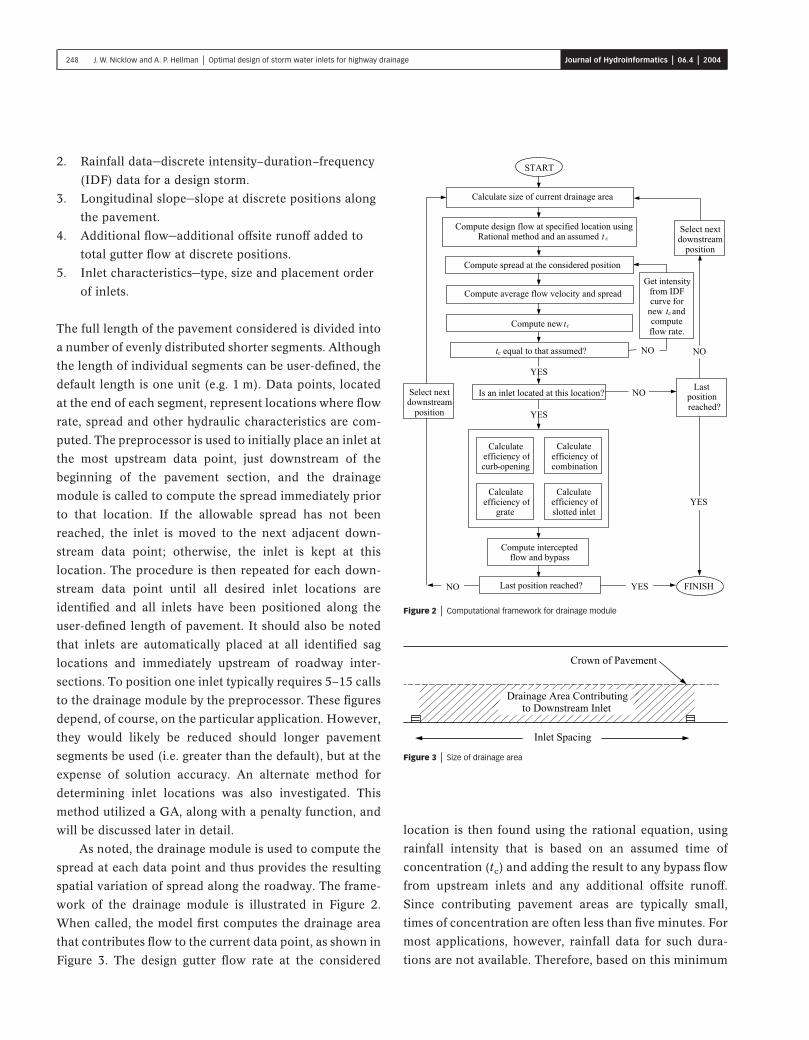
As noted, the drainage module is used to compute the

spread at each data point and thus provides the resulting

spatial variation of spread along the roadway. The frame-

work of the drainage module is illustrated in Figure 2.

When called, the model first computes the drainage area

that contributes flow to the current data point, as shown in

Figure 3. The design gutter flow rate at the considered

location is then found using the rational equation, using

rainfall intensity that is based on an assumed time of

concentration (tc) and adding the result to any bypass flow

from upstream inlets and any additional offsite runoff.

Since contributing pavement areas are typically small,

times of concentration are often less than five minutes. For

most applications, however, rainfall data for such dura-

tions are not available. Therefore, based on this minimum

Figure 2 | Computational framework for drainage module

Figure 3 | Size of drainage area


value recommended by Brown et al. (1996) for design

applications, a value of tc equal to five minutes is initially

assumed.

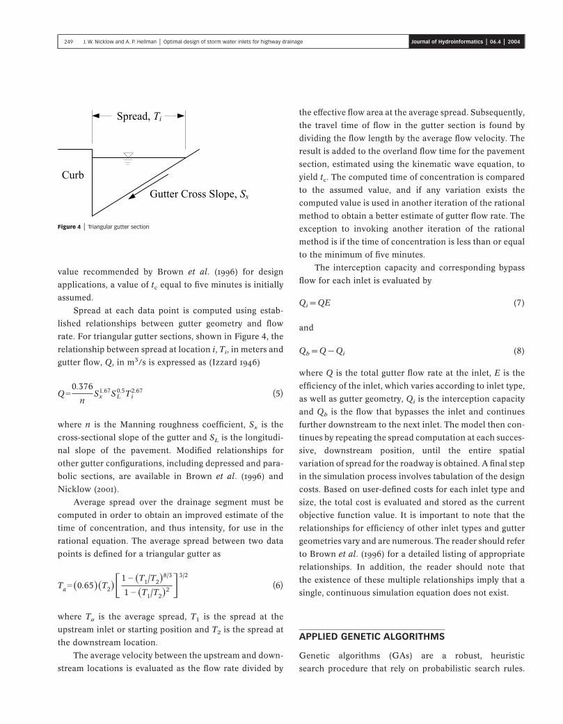
Spread at each data point is computed using estab-

lished relationships between gutter geometry and flow

rate. For triangular gutter sections, shown in Figure 4, the

relationship between spread at location i, Ti, in meters and

gutter flow, Q, in m3/s is expressed as (Izzard 1946)

Q�0.376

nSx

1.67SL0.5T i

2.67 (5)

where n is the Manning roughness coefficient, Sx is the

cross-sectional slope of the gutter and SL is the longitudi-

nal slope of the pavement. Modified relationships for

other gutter configurations, including depressed and para-

bolic sections, are available in Brown et al. (1996) and

Nicklow (2001).

Average spread over the drainage segment must be

computed in order to obtain an improved estimate of the

time of concentration, and thus intensity, for use in the

rational equation. The average spread between two data

points is defined for a triangular gutter as

Ta��0.65��T2�F1��T1/T2�8/3

1��T1/T2�2 G3/2

(6)

where Ta is the average spread, T1 is the spread at the

upstream inlet or starting position and T2 is the spread at

the downstream location.

The average velocity between the upstream and down-

stream locations is evaluated as the flow rate divided by

the effective flow area at the average spread. Subsequently,

the travel time of flow in the gutter section is found by

dividing the flow length by the average flow velocity. The

result is added to the overland flow time for the pavement

section, estimated using the kinematic wave equation, to

yield tc. The computed time of concentration is compared

to the assumed value, and if any variation exists the

computed value is used in another iteration of the rational

method to obtain a better estimate of gutter flow rate. The

exception to invoking another iteration of the rational

method is if the time of concentration is less than or equal

to the minimum of five minutes.

The interception capacity and corresponding bypass

flow for each inlet is evaluated by

Qi = QE (7)

and

Qb = Q − Qi (8)

where Q is the total gutter flow rate at the inlet, E is the

efficiency of the inlet, which varies according to inlet type,

as well as gutter geometry, Qi is the interception capacity

and Qb is the flow that bypasses the inlet and continues

further downstream to the next inlet. The model then con-

tinues by repeating the spread computation at each succes-

sive, downstream position, until the entire spatial

variation of spread for the roadway is obtained. A final step

in the simulation process involves tabulation of the design

costs. Based on user-defined costs for each inlet type and

size, the total cost is evaluated and stored as the current

objective function value. It is important to note that the

relationships for efficiency of other inlet types and gutter

geometries vary and are numerous. The reader should refer

to Brown et al. (1996) for a detailed listing of appropriate

relationships. In addition, the reader should note that

the existence of these multiple relationships imply that a

single, continuous simulation equation does not exist.

APPLIED GENETIC ALGORITHMS

Genetic algorithms (GAs) are a robust, heuristic

search procedure that rely on probabilistic search rules.

Figure 4 | Triangular gutter section


Developed by Holland (1975), they represent an attempt to

adapt the evolution observed in nature to problems in

which traditional, deterministic search techniques have

difficulties. Although there is no rigorous definition that

applies to all GAs, most are at least characterized by the

following common elements: ranking and selection of

solutions according to fitness, crossover to produce new

offspring solutions and random mutation of the new off-

spring (Mitchell 1996; Haupt & Haupt 1998). Through

these elements, GAs simulate survival and generation-

based propagation of those solutions that have the fittest

objective function values (Belegundu & Chandrupatla

1999).

GAs are different from common gradient-based opti-

mization techniques in that they require no derivative

information about the objective function or constraints.

Instead, the objective function magnitude, rather than

derivative terms, is used to display incrementally better

solutions. This characteristic makes GAs amenable for

application to nonconvex, highly nonlinear and even dis-

continuous problems, such as the inlet design problem, for

which traditional optimization techniques would fail

(Goldberg 1989). The method has thus been increasingly

popular for solving optimization and control problems

in a wide variety of fields, including water resources

engineering (see Wang 1991; Esat & Hall 1994; McKinney

& Lin 1994; Ritzel et al. 1994; Oliveira & Loucks 1997; Reis

et al. 1997; Savic & Walters 1997; Wardlaw & Sharif 1999;

Hilton & Culver 2000). For a discussion of the detailed

framework of genetic algorithms, the reader is also

referred to Goldberg (1989), Mitchell (1996) and Haupt &

Haupt (1998).

The GA developed for the inlet design problem begins

by randomly generating an initial population of chromo-

somes, consisting of 25 potential design alternatives. The

size of the population remains constant throughout each

generation of the GA. Although the user is given the

flexibility to change the population size, 25 is a default and

was selected by testing various population ranges and

evaluating the corresponding number of generations

required for solution convergence. In addition, the com-

putational time required for convergence was considered.

A significantly smaller or larger population resulted

in additional generations for convergence without a

corresponding reduction in inlet design cost. Further-

more, larger populations tended to result in excessive, and

often wasteful, computational times. Consider that, for

each chromosome, the drainage simulation module must

be called to evaluate flow characteristics and a resulting

objective function value. Since each module run requires

approximately 30 seconds to execute, the computational

time associated with a larger population quickly increases.

Each member of the initial population is encoded

using an array of positive integers, called genes, which

represent decision variables. Each integer, or gene, is

associated with a particular inlet type and size. The integer

coding is established within a separate database, and when

the integers are sequenced within a chromosome they

describe characteristics of a particular design. For

example, after each available inlet type and size has been

assigned an integer, the chromosome (1287) would indi-

cate that inlet 1, of unique size and type, is the most

upstream inlet. Inlet 2 is the next downstream inlet in the

sequence, followed by inlet 8 and inlet 7. The fitness of

each chromosome is the associated objective function

value (Equation (1)) for the design, retrieved from the

drainage simulation model, and thus represents a suit-

ability metric for solving the optimization problem. This

value establishes the basis for ranking and selection of the

fittest pairs of chromosomes that are mated (i.e. crossover)

to produce improved designs.

Based on their objective function values, the chromo-

somes within the population are ranked in ascending

order. The ten best chromosomes, or those with the lowest

cost, serve as a mating pool from which parents are

selected. Each of these ten designs is first assigned a

ranking number according to a Hoerl power function with

coefficients fitted so that the ten first ranking numbers

sum to unity. The resulting function can be expressed as

Rn = 0.4 × 0.745C C − 0.105 (9)

where Rn is the ranking number and C is a chromosome

between 1 and 10. For example, applying the function to

the best (i.e. first) chromosome yields a ranking number of

0.298, while for the tenth (i.e. last) chromosome, a ranking

of 0.017 is determined. This assigned ranking scheme is

shown graphically in Figure 5. Next, to generate offspring


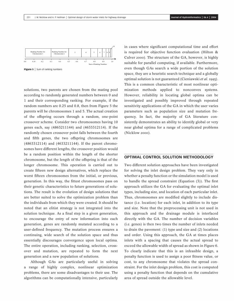
solutions, two parents are chosen from the mating pool

according to randomly generated numbers between 0 and

1 and their corresponding ranking. For example, if the

random numbers are 0.25 and 0.8, then from Figure 5 the

parents will be chromosomes 1 and 5. The actual creation

of the offspring occurs through a random, one-point

crossover scheme. Consider two chromosomes having 10

genes each, say (4863211144) and (4633312114). If the

randomly chosen crossover point falls between the fourth

and fifth genes, the two offspring chromosomes are

(4863312114) and (4633211144). If the parent chromo-

somes have different lengths, the crossover position would

be a random position within the length of the shorter

chromosome, but the length of the offspring is that of the

longer chromosome. This operation is carried out to

create fifteen new design alternatives, which replace the

worst fifteen chromosomes from the initial, or previous,

generation. In this way, the fittest chromosomes pass on

their genetic characteristics to future generations of solu-

tions. The result is the evolution of design solutions that

are better suited to solve the optimization problem than

the individuals from which they were created. It should be

noted that an elitist strategy is not integrated into the

solution technique. As a final step in a given generation,

to encourage the entry of new information into each

generation, genes are randomly mutated according to a

user-defined frequency. The mutation process ensures a

continuing, wide search of the solution space and thus

essentially discourages convergence upon local optima.

The entire operation, including ranking, selection, cross-

over and mutation, are repeated to form the next

generation and a new population of solutions.

Although GAs are particularly useful in solving

a range of highly complex, nonlinear optimization

problems, there are some disadvantages to their use. The

algorithms can be computationally intensive, particularly

in cases where significant computational time and effort

is required for objective function evaluation (Hilton &

Culver 2000). The structure of the GA, however, is highly

suitable for parallel computing, if available. Furthermore,

even though GAs search a wide portion of the solution

space, they are a heuristic search technique and a globally

optimal solution is not guaranteed (Cieniawski et al. 1995).

This is a common characteristic of most nonlinear opti-

mization methods applied to nonconvex systems.

However, reliability in locating global optima can be

investigated and possibly improved through repeated

sensitivity applications of the GA in which the user varies

parameters such as population size and mutation fre-

quency. In fact, the majority of GA literature con-

sistently demonstrates an ability to identify global or very

near global optima for a range of complicated problems

(Nicklow 2000).

OPTIMAL CONTROL SOLUTION METHODOLOGY

Two different solution approaches have been investigated

for solving the inlet design problem. They vary only in

whether a penalty function or the simulation model is used

to handle the spread constraint (Equation (3)). The first

approach utilizes the GA for evaluating the optimal inlet

types, including size, and location of each particular inlet.

Thus, chromosomes are modified slightly to include dis-

tance (i.e. location) for each inlet, in addition to its type

and size. Note that the preprocessing unit is not used in

this approach and the drainage module is interfaced

directly with the GA. The number of decision variables

(i.e. genes) is then two times the number of inlets needed

to drain the pavement: (1) type and size and (2) locations

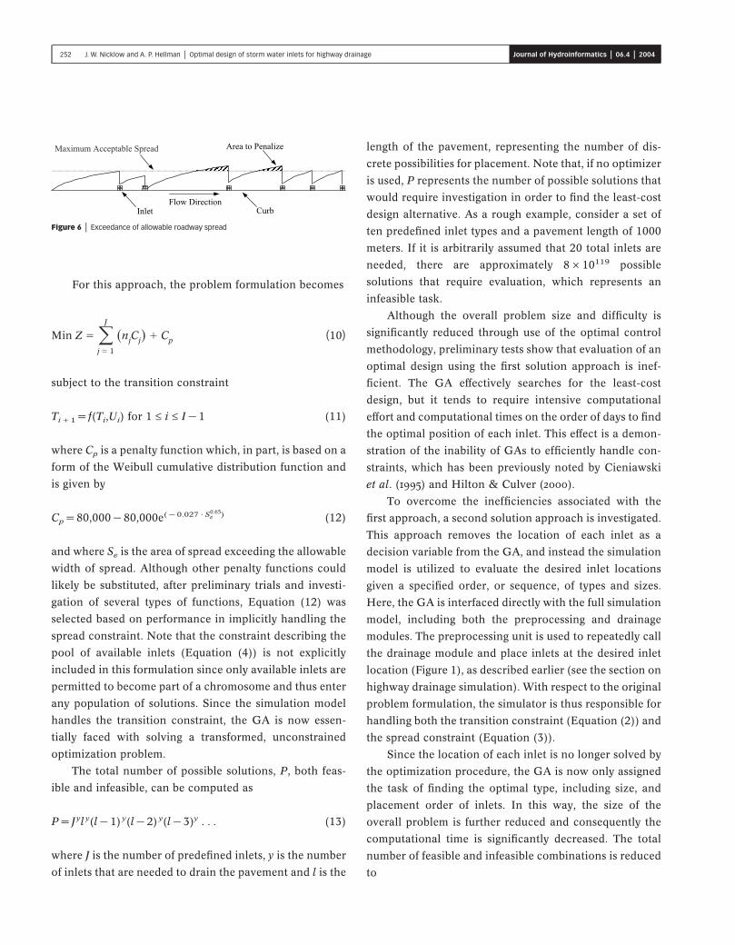
and order. Using this approach, the GA at times places

inlets with a spacing that causes the actual spread to

exceed the allowable width of spread as shown in Figure 6.

To clearly indicate that this is an infeasible design, a

penalty function is used to assign a poor fitness value, or

cost, to any chromosome that violates the spread con-

straint. For the inlet design problem, this cost is computed

using a penalty function that depends on the cumulative

area of spread outside the allowable level.

Figure 5 | Sum of ranking numbers


For this approach, the problem formulation becomes

Min Z � ∑j � 1

J

�njCj� � Cp (10)

subject to the transition constraint

Ti + 1 = f(Ti,Ui) for 1 ≤ i ≤ I − 1 (11)

where Cp is a penalty function which, in part, is based on a

form of the Weibull cumulative distribution function and

is given by

Cp = 80,000 − 80,000e( − 0.027 · S0.65)e (12)

and where Se is the area of spread exceeding the allowable

width of spread. Although other penalty functions could

likely be substituted, after preliminary trials and investi-

gation of several types of functions, Equation (12) was

selected based on performance in implicitly handling the

spread constraint. Note that the constraint describing the

pool of available inlets (Equation (4)) is not explicitly

included in this formulation since only available inlets are

permitted to become part of a chromosome and thus enter

any population of solutions. Since the simulation model

handles the transition constraint, the GA is now essen-

tially faced with solving a transformed, unconstrained

optimization problem.

The total number of possible solutions, P, both feas-

ible and infeasible, can be computed as

P = Jyl y(l − 1) y(l − 2) y(l − 3)y . . . (13)

where J is the number of predefined inlets, y is the number

of inlets that are needed to drain the pavement and l is the

length of the pavement, representing the number of dis-

crete possibilities for placement. Note that, if no optimizer

is used, P represents the number of possible solutions that

would require investigation in order to find the least-cost

design alternative. As a rough example, consider a set of

ten predefined inlet types and a pavement length of 1000

meters. If it is arbitrarily assumed that 20 total inlets are

needed, there are approximately 8 × 10119 possible

solutions that require evaluation, which represents an

infeasible task.

Although the overall problem size and difficulty is

significantly reduced through use of the optimal control

methodology, preliminary tests show that evaluation of an

optimal design using the first solution approach is inef-

ficient. The GA effectively searches for the least-cost

design, but it tends to require intensive computational

effort and computational times on the order of days to find

the optimal position of each inlet. This effect is a demon-

stration of the inability of GAs to efficiently handle con-

straints, which has been previously noted by Cieniawski

et al. (1995) and Hilton & Culver (2000).

To overcome the inefficiencies associated with the

first approach, a second solution approach is investigated.

This approach removes the location of each inlet as a

decision variable from the GA, and instead the simulation

model is utilized to evaluate the desired inlet locations

given a specified order, or sequence, of types and sizes.

Here, the GA is interfaced directly with the full simulation

model, including both the preprocessing and drainage

modules. The preprocessing unit is used to repeatedly call

the drainage module and place inlets at the desired inlet

location (Figure 1), as described earlier (see the section on

highway drainage simulation). With respect to the original

problem formulation, the simulator is thus responsible for

handling both the transition constraint (Equation (2)) and

the spread constraint (Equation (3)).

Since the location of each inlet is no longer solved by

the optimization procedure, the GA is now only assigned

the task of finding the optimal type, including size, and

placement order of inlets. In this way, the size of the

overall problem is further reduced and consequently the

computational time is significantly decreased. The total

number of feasible and infeasible combinations is reduced

to

Figure 6 | Exceedance of allowable roadway spread


P = J y. (14)

For this case, a set of ten predefined inlets and a pavement

length that requires 20 total inlets yield 1020 possible

designs, which represents a significant reduction com-

pared to the first approach. Based on preliminary tests and

a comparison of solution approaches, this second

approach has been selected for further use in the optimal

control model.

EXAMPLE APPLICATION

To demonstrate the capabilities of the new methodology,

the optimal control model is applied to a hypothetical, yet

realistic, roadway system that is similar to those found in

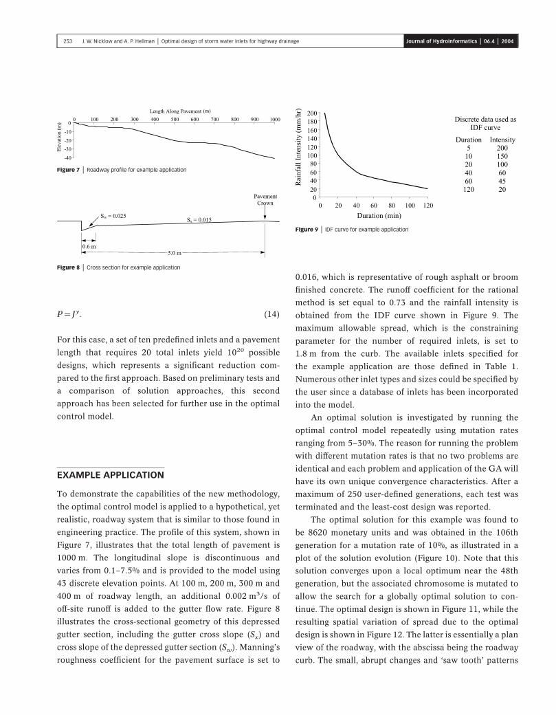
engineering practice. The profile of this system, shown in

Figure 7, illustrates that the total length of pavement is

1000 m. The longitudinal slope is discontinuous and

varies from 0.1–7.5% and is provided to the model using

43 discrete elevation points. At 100 m, 200 m, 300 m and

400 m of roadway length, an additional 0.002 m3/s of

off-site runoff is added to the gutter flow rate. Figure 8

illustrates the cross-sectional geometry of this depressed

gutter section, including the gutter cross slope (Sx) and

cross slope of the depressed gutter section (Sw). Manning’s

roughness coefficient for the pavement surface is set to

0.016, which is representative of rough asphalt or broom

finished concrete. The runoff coefficient for the rational

method is set equal to 0.73 and the rainfall intensity is

obtained from the IDF curve shown in Figure 9. The

maximum allowable spread, which is the constraining

parameter for the number of required inlets, is set to

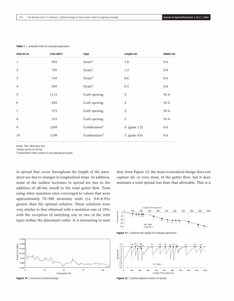
1.8 m from the curb. The available inlets specified for

the example application are those defined in Table 1.

Numerous other inlet types and sizes could be specified by

the user since a database of inlets has been incorporated

into the model.

An optimal solution is investigated by running the

optimal control model repeatedly using mutation rates

ranging from 5–30%. The reason for running the problem

with different mutation rates is that no two problems are

identical and each problem and application of the GA will

have its own unique convergence characteristics. After a

maximum of 250 user-defined generations, each test was

terminated and the least-cost design was reported.

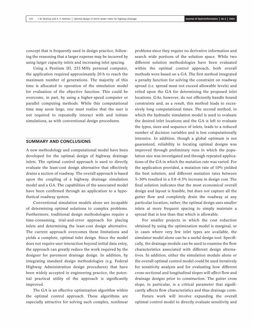
The optimal solution for this example was found to

be 8620 monetary units and was obtained in the 106th

generation for a mutation rate of 10%, as illustrated in a

plot of the solution evolution (Figure 10). Note that this

solution converges upon a local optimum near the 48th

generation, but the associated chromosome is mutated to

allow the search for a globally optimal solution to con-

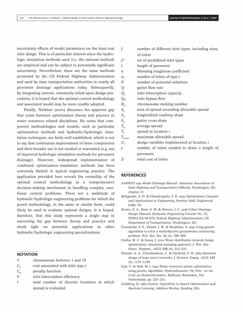
tinue. The optimal design is shown in Figure 11, while the

resulting spatial variation of spread due to the optimal

design is shown in Figure 12. The latter is essentially a plan

view of the roadway, with the abscissa being the roadway

curb. The small, abrupt changes and ‘saw tooth’ patterns

Figure 7 | Roadway profile for example application

Figure 8 | Cross section for example application

Figure 9 | IDF curve for example application


in spread that occur throughout the length of the pave-

ment are due to changes in longitudinal slope. In addition,

some of the sudden increases in spread are due to the

addition of off-site runoff to the total gutter flow. Tests

using other mutation rates converged to values that were

approximately 70–560 monetary units (i.e. 0.8–6.5%)

greater than the optimal solution. These solutions were

very similar to that obtained with a mutation rate of 10%,

with the exception of switching one or two of the inlet

types within the placement order. It is interesting to note

that, from Figure 12, the most economical design does not

capture all, or even most, of the gutter flow, but it does

maintain a total spread less than that allowable. This is a

Table 1 | Available inlets for example application

Inlet ID no. Cost (MU1) Type Length (m) Width (m)

1 845 Grate2 1.8 0.6

2 795 Grate2 1.2 0.6

3 745 Grate2 0.6 0.6

4 695 Grate2 0.3 0.6

5 1115 Curb opening 5 N/A




9 1249 Combination3 4 (grate 1.2) 0.6

10 1199 Combination2 3 (grate 0.6) 0.6

Notes: 1MU=Monetary Unit.2Grates are 30–85 tilt bar.3Combination inlets consist of curb opening and grate.

Figure 10 | Evolution of optimal design

Figure 11 | Optimal inlet design for example application

Figure 12 | Optimal spatial variation of spread


concept that is frequently used in design practice, follow-

ing the reasoning that a larger expense may be incurred by

using larger capacity inlets and increasing inlet spacing.

Using a Pentium III, 233 MHz personal computer,

the application required approximately 20 h to reach the

maximum number of generations. The majority of this

time is allocated to operation of the simulation model

for evaluation of the objective function. This could be

overcome, in part, by using a higher-speed computer or

parallel computing methods. While this computational

time may seem large, one must realize that the user is

not required to repeatedly interact with and initiate

simulations, as with conventional design procedures.

SUMMARY AND CONCLUSIONS

A new methodology and computational model have been

developed for the optimal design of highway drainage

inlets. The optimal control approach is used to directly

evaluate the least-cost design alternative that effectively

drains a section of roadway. The overall approach is based

upon the coupling of a highway drainage simulation

model and a GA. The capabilities of the associated model

have been confirmed through an application to a hypo-

thetical roadway system.

Conventional simulation models alone are incapable

of determining optimal solutions to complex problems.

Furthermore, traditional design methodologies require a

time-consuming, trial-and-error approach for placing

inlets and determining the least-cost design alternative.

The current approach overcomes these limitations and

yields a complete, optimal inlet design. Since the model

does not require user interaction beyond initial data entry,

the approach can greatly reduce the work required by the

designer for pavement drainage design. In addition, by

integrating standard design methodologies (e.g. Federal

Highway Administration design procedures) that have

been widely accepted in engineering practice, the poten-

tial practical utility of the approach is significantly

improved.

The GA is an effective optimization algorithm within

the optimal control approach. These algorithms are

especially attractive for solving such complex, nonlinear

problems since they require no derivative information and

search wide portions of the solution space. While two

different solution methodologies have been evaluated

within the optimal control approach, both overall

methods were based on a GA. The first method integrated

a penalty function for solving the constraint on roadway

spread (i.e. spread must not exceed allowable levels) and

relied upon the GA for determining the proposed inlet

locations. GAs, however, do not efficiently handle bound

constraints and, as a result, this method leads to exces-

sively long computational times. The second method, in

which the hydraulic simulation model is used to evaluate

the desired inlet locations and the GA is left to evaluate

the types, sizes and sequence of inlets, leads to a reduced

number of decision variables and is less computationally

intensive. In addition, though a global optimum is not

guaranteed, reliability in locating optimal designs was

improved through preliminary runs in which the popu-

lation size was investigated and through repeated applica-

tions of the GA in which the mutation rate was varied. For

the application provided, a mutation rate of 10% yielded

the best solution, and different mutation rates between

5–30% resulted in a 0.8–6.5% increase in design cost. The

final solution indicates that the most economical overall

design and layout is feasible, but does not capture all the

gutter flow and completely drain the roadway at any

particular location; rather, the optimal design uses smaller

inlets at more frequent spacing to simply maintain a

spread that is less than that which is allowable.

For smaller projects in which the cost reduction

obtained by using the optimization model is marginal, or

in cases where very few inlet types are available, the

simulator model alone can be a useful design tool. Specifi-

cally, the drainage module can be used to examine the flow

characteristics associated with different design alterna-

tives. In addition, either the simulation module alone or

the overall optimal control model could be used iteratively

for sensitivity analysis and for evaluating how different

cross-sectional and longitudinal slopes will affect flow and

drainage designs prior to construction. The gutter cross

slope, in particular, is a critical parameter that signifi-

cantly affects flow characteristics and thus drainage costs.

Future work will involve expanding the overall

optimal control model to directly evaluate sensitivity and


uncertainty effects of model parameters on the least-cost

inlet design. This is of particular interest since the hydro-

logic simulation methods used (i.e. the rational method)

are empirical and can be subject to potentially significant

uncertainty. Nevertheless, these are the same methods

promoted by the US Federal Highway Administration

and used by state transportation authorities in nearly all

pavement drainage applications today. Subsequently,

by integrating current, commonly relied upon design pro-

cedures, it is hoped that the optimal control methodology

and associated model may be more readily adopted.

Finally, Nicklow (2000) discusses the apparent gap

that exists between optimization theory and practice in

water resources related disciplines. He notes that com-

ponent methodologies and models, such as particular

optimization methods and hydraulic/hydrologic simu-

lation techniques, are fairly well established, which is not

to say that continuous improvement of these components

and their broader use is not needed or warranted (e.g. use

of improved hydrologic simulation methods for pavement

drainage). However, widespread implementation of

combined optimization–simulation methods has been

extremely limited in typical engineering practice. The

application provided here reveals the versatility of the

optimal control methodology as a comprehensive

decision-making mechanism in handling complex, non-

linear control problems. There are a multitude of

hydraulic/hydrologic engineering problems for which the

posed methodology, in the same or similar form, could

likely be used to evaluate optimal designs. It is hoped,

therefore, that this study represents a single step in

narrowing the gap between theory and practice and

sheds light on potential applications in other

hydraulic/hydrologic engineering specializations.

NOTATIONC chromosome between 1 and 10

Cj cost associated with inlet type j

Cp penalty function

E inlet interception efficiency

I total number of discrete locations at which

spread is evaluated

J number of different inlet types, including sizes,

of inlets

J* set of predefined inlet types

l length of pavement

n Manning roughness coefficient

nj number of inlets of type j

P number of potential solutions

Q gutter flow rate

Qi inlet interception capacity

Qb inlet bypass flow

Rn chromosome ranking number

Se area of spread exceeding allowable spread

SL longitudinal roadway slope

Sx gutter cross slope

Ta average spread

Ti spread at location i

Tmax maximum allowable spread

Ui design variables implemented at location i

y number of inlets needed to drain a length of

pavement

Z total cost of inlets

REFERENCES

AASHTO 1991 Model Drainage Manual. American Association ofState Highway and Transportation Officials, Washington, DC,chapter 13.

Belegundu, A. D. & Chandrupatla, T. R. 1999 Optimization Conceptsand Applications in Engineering, Prentice Hall, EnglewoodCliffs, NJ.

Brown, S. A., Stein, S. M. & Warner, J. C. 1996 Urban DrainageDesign Manual, Hydraulic Engineering Circular No. 22,FHWA-SA-96-078, Federal Highway Administration, USDepartment of Transportation, Washington, DC.

Cieniawski, S. E., Eheart, J. W. & Ranjithan, S. 1995 Using geneticalgorithms to solve a multiobjective groundwater monitoringproblem. Wat. Res. Res. 31 (2), 399–409.

Cunha, M. C. & Sousa, J. 2000 Water distribution network designoptimization: simulated annealing approach. J. Wat. Res.Plann. Mngmnt., ASCE 125 (4), 215–221.

Elimam, A. A., Charalambous, C. & Ghobrial, F. H. 1989 Optimumdesign of large sewer networks. J. Environ. Engng, ASCE 115(6), 1170–1190.

Esat, V. & Hall, M. J. 1994 Water resources system optimisationusing genetic algorithms. Hydroinfomatics ’94, Proc. 1st Int.Conf. on Hydroinformatics. Balkema, Rotterdam, TheNetherlands, pp. 225–231.

Goldberg, D. 1989 Genetic Algorithms in Search Optimization andMachine Learning. Addison-Wesley, Reading, MA.


Haupt, R. L. & Haupt, S. E. 1998 Practical Genetic Algorithms.Wiley, New York.

Hilton, A. C. & Culver, T. B. 2000 Constraint handling for geneticalgorithms in optimal remediation design. J. Wat. Res. Plann.Mngmnt., ASCE 126 (3), 128–137.

Holland, J. H. 1975 Adaptation in Natural and Artificial Systems.University of Michigan Press, Ann Arbor, MI.

IDOT. 1989 Drainage Manual. Illinois Department ofTransportation, Bureau of Bridges and Structures,Springfield, IL.

Izzard, C. F. 1946 Hydraulics of Runoff from Developed Surfaces,Proc. Highway Research Board, vol. 26. Highway ResearchBoard, Washington, DC, pp. 129–150.

Johnson, F. L. & Chang, F. M. 1984 Drainage of HighwayPavements, Hydraulic Engineering Circular No. 12,FHWA-TS-84-202. Federal Highway Administration, USDepartment of Transportation, Washington, DC.

Li, G. & Matthew, R. G. S. 1990 New approach for optimization ofurban drainage systems. J. Environ. Engng, ASCE 116 (5),927–944.

Mays, L. W. 1979 Optimal design of culverts under uncertainties.J. Hydraul. Engng, ASCE 105 (HY5), 443–460.

McKinney, D. C. & Lin, M. D. 1994 Genetic algorithm solution ofgroundwater management models. Wat. Res. Res. 30 (6),1897–1906.

Minsker, B. S. & Shoemaker, C. A. 1998 Dynamic optimal control ofin-situ bioremediation of ground water. J. Wat. Res. Plann.Mngmnt, ASCE 124 (3), 149–161.

Mitchell, M. 1996 An Introduction to Genetic Algorithms. MITPress, Cambridge, MA.

Nicklow, J. W. 2000 Discrete-time optimal control for waterresources engineering and management. Wat. Int. 25 (1),89–95.

Nicklow, J. W. 2001 Design of storm water inlets. In Storm WaterCollection Systems Handbook (ed. Mays, L. W.). McGraw-Hill,New York, Chapter 5.

Nicklow, J. W. & Mays, L. W. 2000 Optimization of multiplereservoir networks for sedimentation control. J. Hydraul.Engng, ASCE 126 (4), 232–242.

Oliveira, R. & Loucks, D. P. 1997 Operating rules for multireservoirsystems. Wat. Res. Res. 33 (4), 839–852.

Reis, L. F. R., Porto, R. M. & Chaudhry, F. H. 1997 Optimal locationof control valves in pipe networks by genetic algorithm. J. Wat.Res. Plann. Mngmnt, ASCE 123 (6), 317–320.

Ritzel, B. J., Eheart, J. W. & Ranjithan, S. 1994 Using geneticalgorithms to solve a multiple objective groundwater pollutionproblem. Wat. Res. Res. 30 (5), 1589–1603.

Sakarya, A. B. & Mays, L. W. 2000 Optimal operation of waterdistribution pumps considering water quality. J. Wat. Res.Plann. Mngmnt., ASCE 126 (4), 210–220.

Savic, D. A. & Walters, G. A. 1997 Genetic algorithms for least-costdesign of water distribution networks. J. Wat. Res. Plann.Mngmnt, ASCE 123 (2), 67–77.

Templeman, A. B. & Walters, G. A. 1979 Optimal design ofstormwater drainage networks for roads. Proc. ICE, Part I –Design and Construction, vol 67. Institute of Civil Engineers,New York, pp. 573–587.

Unver, O. I. & Mays, L. W. 1990 Model for real-time optimal floodcontrol operation of a reservoir system. Wat. Res. Mngmnt 4,21–46.

Wanakule, N., Mays, L. W. & Lasdon, L. S. 1986 Optimalmanagement of large-scale aquifers: methogology andapplication. Wat. Res. Res. 22 (4), 447–465.

Wang, Q. J. 1991 The genetic algorithm and its application tocalibration conceptual rainfall-runoff models. Wat. Res. Res.27 (9), 2467–2471.

Wardlaw, R. & Sharif, M. 1999 Evaluation of genetic algorithms foroptimal reservoir system operation. J. Wat. Res. Plann.Mngmnt, ASCE 125 (1), 25–33.

Yeh, W. W.-G. 1985 Reservoir management and operations models:a state-of-the-art review. Wat. Res. Res. 21 (12), 1797–1818.

Yeh, W. W.-G. 1992 Systems analysis in ground-water planning andmanagement. J. Wat. Res. Plann. Mngmnt, ASCE 118 (3),224–237.


Documents

Optimal design of storm water inlets for highway drainagejh.iwaponline.com/content/ppiwajhydro/6/4/245.full.pdf · Optimal design of storm water inlets for highway drainage ... evaluated