i

Optimal Design of Levee and Flood Control Systems

By

RUI HUI

B.S. (Tsinghua University, China) 2011 M.S. (University of California, Davis, U.S.) 2013

DISSERTATION

Submitted in partial satisfaction of the requirements for the degree of

DOCTOR OF PHILOSOPHY

in

Civil and Environmental Engineering

in the OFFICE OF GRADUATE STUDIES

of the

UNIVERSITY OF CALIFORNIA DAVIS

Approved:

_____________________________________

Jay R. Lund, Chair

_____________________________________

Bassam Younis

_____________________________________

Samuel Sandoval Solis

Committee in Charge

2014

ii

Acknowledgements I have worked with a couple of people who contributed a lot to the research and this

dissertation. I really appreciate their help in all aspects.

I would first like to thank Prof. Jay R. Lund, my major advisor and committee chair, for his help, support, encouragement, and guidance throughout my dissertation and my entire graduate study. His kindness, enthusiasm and insight make working with him full of joy. I am grateful to have him as an advisor and friend.

My dissertation committee members, Prof. Bassam Younis and Prof. Samuel Sandoval Solis, have offered continued support and counsel throughout the writing of this dissertation. Their knowledge and passion inspire me in my career. I would also like to thank Prof. Yueyue Fan and Prof. Kevin Novan for their advice. Thanks go to Prof. Kaveh Madani for valuable suggestions on the game theory study, and to Prof. Jianshi Zhao for his comments on the flood hedging study.

During my daily study and research, I have received continuous support from former and current research group members, in particular, Josué Medellín-Azuara, Alvar Escriva-Bou, Tingju Zhu, Patric Ji, Prudentia Zikalala and Elizabeth Jachens, for their many helps. I have to thank all my dear friends who are supporting me, in particular, Barbara Bellieu, Cathryn A. Lawrence, Xiaonan Wang, Yipeng Lu, Lizhi Tao, Yating Yang, Lixin Wang, Xingyu Duan, Ying Luo and Wei Jia. My life in graduate school wouldn’t be so colorful without them.

Finally, I would like to thank my family. Words cannot express my gratitude for my parents, my father Quanguo Hui and my mother Shuxia Geng. I particularly want to thank my husband, Bo Guo, for his love, patience and understanding. I have been blessed with encouragement, support, guidance, and unconditional love throughout my entire life. I would not be where I am today without them. They are my role models and friends.

iii

Abstract Flooding often threatens riverine and coastal areas, particularly urbanized flood-prone areas

that are densely populated and high-valued, which causes damages to life, property, society and the economy. Upstream flood reservoir operations and downstream levee construction are two common ways to protect from flooding. Most traditional risk-based analyses for optimal levee design focus primarily on overtopping failure, and few risk analysis studies explicitly include the more frequently observed intermediate geotechnical failures. This study first develops a risk-based optimization model for single levee designs given two simplified levee failure modes: overtopping and overall intermediate geotechnical failures. The optimization minimizes the annual expected total cost, which sums the expected annual damage cost and annualized construction cost. This optimization model is then extended to examine a common simple levee system with levees on opposite riverbanks, allowing flood risk transfer across the river. The economic optimality of asymmetric levee system is demonstrated mathematically and analytically, for overtopping failure, overall intermediate geotechnical failure and a combination of failure modes. Where residual flood risk is completely transferred to the low-valued riverbank at economic optimality, individuals may be compensated for the transferred flood risk to guarantee and improve outcomes for all parties. Such collaborative designs of the two levee system are economically optimal for the whole system. However, rational and self-interested land owners that control levees on each river bank separately often tend to independently optimize their levees. By applying game theory to the simple levee system, the cooperative game with a system-wide economically optimal design and the single-shot non-cooperative Nash equilibrium are identified, and the successive repeated non-cooperative reversible and irreversible games are examined. Compensation for the transferred flood risk can be determined by comparing different types of games and implemented with land owners’ agreements on allocations of flood risk and benefits. The resulting optimized flood risks to a downstream leveed area would further affect the upstream reservoir’s operation in optimizing flood hedging pre-releases, which would create a small flood downstream by pre-storm release to reduce the likelihood of a larger more damaging flood in the future. Overall damages from flood pre-release decisions must be convex for flood hedging to be optimal. Some theoretical conditions for optimal flood hedging are explored: the fundamental one is that the current marginal damages from pre-releases equals the future marginal expected damages from storm releases. Any additional economic water supply lost from pre-releases tends to reduce the use of hedging pre-release for flood management.

iv

Table of Contents

Acknowledgements ................................................................................................................................. ii Abstract ................................................................................................................................................... iii Table of Contents ................................................................................................................................... iv Figures ..................................................................................................................................................... vi Tables .................................................................................................................................................... viii

Introduction ................................................................................................................................... 1

Chapter 1: Risk-Based Analysis for Optimal Single Levee Design .......................................... 4 1.1 Summary ............................................................................................................................................ 4 1.2 Introduction ....................................................................................................................................... 4 1.3 Risk-based Optimization for a Single Levee ................................................................................... 5

1.3.1 Model Description ....................................................................................................................... 5 1.3.2 Intermediate Geotechnical Levee Failure .................................................................................... 6 1.3.3 Risk-based Optimization Model .................................................................................................. 9

1.4 Model Applications ......................................................................................................................... 10 1.4.1 Model Applications in A Small Rural Levee on Cosumnes River ............................................ 10 1.4.2 Model Applications in A Large Urban Natomas Levee on Sacramento River .......................... 16

1.5 Sensitivity Analysis ......................................................................................................................... 19 1.5.1 Impacts from Levee Fragility Curves ........................................................................................ 19 1.5.2 Analytical View of Trader-off in Design Parameter .................................................................. 21

1.6 Conclusion ....................................................................................................................................... 22 1.7 References ........................................................................................................................................ 23

Chapter 2: Risk-Based Analysis for Optimal Simple Levee System Design ......................... 25 2.1 Summary .......................................................................................................................................... 25 2.2 Introduction ..................................................................................................................................... 25 2.3 Risk-based Optimization Model for a Simple Levee System ...................................................... 26

2.3.1 Model Description ..................................................................................................................... 26 2.3.2 Risk-based Optimization for Overtopping Levee Failure Only ................................................. 27 2.3.3 Risk-based Optimization for Intermediate Geotechnical Levee Failure Only ........................... 30 2.3.4 Risk-based Optimization for Overtopping and Intermediate Geotechnical Failures ................. 33

2.4 Illustrative Examples ...................................................................................................................... 38 2.4.1 Applications in A Small Levee on Cosumnes River .................................................................. 38 2.4.2 Applications in A Large Levee on Sacramento River ............................................................... 40

2.5 Conclusion ....................................................................................................................................... 42 2.6 References ........................................................................................................................................ 42 2.7 Appendixes ....................................................................................................................................... 42

2.7.A Economic Optimality of the Asymmetric Levee Height ........................................................... 42 2.7.B Optimal Levee Height of the Asymmetric Levee Height .......................................................... 44 2.7.C Economic Optimality of the Asymmetric Levee Crown Width ................................................ 51 2.7.D Economic Optimality of the Asymmetric Levee System Geometry ......................................... 53

Chapter 3: Game Theory and Risk-Based Levee System Design ........................................... 57 3.1 Summary .......................................................................................................................................... 57 3.2 Introduction ..................................................................................................................................... 57 3.3 Risk-based Optimal Levee Design and Game Theory Framework ............................................ 58

3.3.1 Model Description ..................................................................................................................... 59 3.3.2 Risk-based Optimization for the Whole Levee System ............................................................. 60 3.3.3 A Simple Game Theory Framework .......................................................................................... 61

v

3.3.4 Illustrating Cases ........................................................................................................................ 64 3.4 Cooperative Design ......................................................................................................................... 64 3.5 Single-shot Non-cooperative Game: Nash Equilibrium .............................................................. 65

3.5.1 Identical Floodplain Conditions on Opposite Riverbanks ......................................................... 66 3.5.2 Different Floodplain Conditions on Opposite Riverbanks ......................................................... 68

3.6 Successive Repeated Non-cooperative Game: Reversible Decision Making Mode ................... 71 3.6.1 Identical Floodplain Conditions on Opposite Riverbanks ......................................................... 72 3.6.2 Different Floodplain Conditions on Opposite Riverbanks ......................................................... 74

3.7 Successive Repeated Non-cooperative Game: Irreversible Decision Making Mode ................. 77 3.7.1 Identical Floodplain Conditions on Opposite Riverbanks ......................................................... 77 3.7.2 Different Floodplain Conditions on Opposite Riverbanks ......................................................... 80

3.8 Discussions and Conclusions .......................................................................................................... 81 3.9 References ........................................................................................................................................ 82

Chapter 4: Optimal Flood Pre-release—flood hedging for a single reservoir ...................... 84 4.1 Summary .......................................................................................................................................... 84 4.2 Introduction ..................................................................................................................................... 84 4.3 Simple Optimization Formulation ................................................................................................. 85

4.3.1 Model Description ..................................................................................................................... 85 4.3.2 Mathematical Optimization Formulation ................................................................................... 88 4.3.3 Small, Intermediate and Large Storms ....................................................................................... 90

4.4 Theoretical Optima ......................................................................................................................... 92 4.4.1 KKT Optimality Conditions and Lagrange Multiplier ............................................................... 92 4.4.2 Derivation of Theoretical Optimal Conditions .......................................................................... 92

4.5 Illustrative Examples ...................................................................................................................... 95 4.5.1 Model Inputs .............................................................................................................................. 95 4.5.2 Results for Different Failure Probability Functions ................................................................... 96 4.5.3 Comparisons and Discussions .................................................................................................. 100

4.6 Optimal Flood Hedging with Water Supply Losses and Blended Hedging ............................. 102 4.7 Conclusions and Discussions ........................................................................................................ 106 4.8 References ...................................................................................................................................... 106 4.9 Appendix ........................................................................................................................................ 107

Conclusions ................................................................................................................................ 109

vi

Figures

Figure 1.1 Idealized cross-section of a channel with a single levee ..................................................... 6 Figure 1.2 Sample conceptual levee fragility curves for levees in various conditions ......................... 7 Figure 1.3 Levee failure probability curves for minimum and maximum levee crown widths in

various levee conditions ................................................................................................................ 9 Figure 1.4 Annual expected total costs, annualized construction costs and expected annual damage

costs for different levee crown widths, assuming fair levee condition (rural levee) ................... 11 Figure 1.5 Annual expected total costs, annualized construction costs and expected annual damage

costs for different levee heights, assuming fair levee condition (rural levee) ............................. 12 Figure 1.6 Annual expected total costs for various levee geometries under good, fair and poor levee

conditions (rural levee) ............................................................................................................... 13 Figure 1.7 Contour plots of annual expected total costs for various levee geometries under different

levee conditions (rural levee) ...................................................................................................... 14 Figure 1.8 Annual expected total costs, annualized construction costs and expected annual damage

costs for overtopping failure only and a combination of overtopping and intermediate geotechnical failure, assuming fair levee condition (rural levee) ............................................... 16

Figure 1.9 19 miles of levee on the Sacramento River protecting Natomas Basin to the East ........... 17 Figure 1.10 Levee fragility curves with different curvatures .............................................................. 19

Figure 2.1 Idealized cross-section of leveed river channel system with two levees on opposite

riverbanks .................................................................................................................................... 26 Figure 2.2 Profile view of varying levee height relationships ............................................................ 27 Figure 2.3 Profile view of varying levee condition relationships ....................................................... 31 Figure 2.4 Profile view of varying levee geometries relationships ..................................................... 35 Figure 2.5 Optimal levee heights for symmetric levee system and asymmetric levee system with

short rural levee failing based on optimal conditions or economically marginal theory. ............ 48 Figure 2.6 Optimal levee heights for symmetric levee system with each levee fails at a 50% chance

and asymmetric levee system with short rural levee fails based on optimal conditions or economically marginal theory ..................................................................................................... 51

Figure 3.1 Idealized cross-section of leveed river channel system with two levees on opposite

riverbanks .................................................................................................................................... 59 Figure 3.2 Profile view of varying levee height relationships ............................................................ 60 Figure 3.3 Variation of optimal levee height and annual expected total cost with different damage

potentials in a single levee design case ....................................................................................... 63 Figure 3.4 Best levee height responses of each floodplain with different design levee height

increments, for identical floodplains ........................................................................................... 68 Figure 3.5 Best levee heights of each floodplain with different design levee height increments, for

different floodplains .................................................................................................................... 70 Figure 3.6 Successive repeated levee system design problem in a reversible leader-follower and

simultaneous decision making mode, for identical floodplains .................................................. 73 Figure 3.7 Best response curves in the successive repeated levee system design problem in a

reversible decision making mode, for identical floodplains ....................................................... 74 Figure 3.8 Successive repeated levee system design problem in a reversible leader-follower and

simultaneous decision making mode, for different floodplains .................................................. 76 Figure 3.9 Best response curves in the successive repeated levee system design problem in a

reversible decision making mode, for different floodplains ....................................................... 76

vii

Figure 3.10 Successive repeated levee system design problem in an irreversible leader-follower decision making mode with 1ft levee height increment, for identical floodplains ..................... 78

Figure 3.11 Successive repeated levee system design problem in an irreversible simultaneous decision making mode, for identical floodplains ........................................................................ 79

Figure 3.12 Successive repeated levee system design problem in an irreversible leader-follower decision making mode with 1ft levee height increment, for different floodplains ..................... 80

Figure 3.13 Successive repeated levee system design problem in an irreversible simultaneous decision making mode, for different floodplains ........................................................................ 81

Figure 4.1 Schematic for simple flood hedging .................................................................................. 86 Figure 4.2 Failure probability of town levee with pre-release flow Q ................................................ 87 Figure 4.3 Antecedent flow and flood flow ........................................................................................ 87 Figure 4.4 Standard minimize flooding frequency policy (thicker line) and possible Flood Hedging

Rules ........................................................................................................................................... 88 Figure 4.5 Variation of likely release risk to downstream levees with storm volume, storm releases

follow standard minimize flooding frequency policy ................................................................. 91 Figure 4.6 Failure probabilities of pre-release and resulting storm releases, Convex F(Q) ................ 98 Figure 4.7 Failure probabilities of pre-release and resulting storm releases, Linear F(Q) .................. 99 Figure 4.8 Failure probabilities of pre-release and resulting storm releases, Concave F(Q) ............ 100 Figure 4.9 Optimal flood hedging pre-releases with different economic water supply release ........ 103 Figure 4.10 Hedging Rules for water supply and flood control, standard water supply operating

policy (dashed thicker line) and minimize flooding frequency policy (thicker line) ................ 105

viii

Tables

Table 1.1 Optimal results and comparison for different levee conditions (rural levee) ...................... 15 Table 1.2 Optimal results and comparison for different levee conditions (urban levee) .................... 18 Table 1.3 Sensitivity Analysis on Levee Fragility Curves for good levee conditions (rural levee) .... 20 Table 1.4 Sensitivity Analysis on Levee Fragility Curves for poor levee conditions (rural levee) ..... 21

Table 2.1 Comparison of Four Potential Consequences for A Simple Levee System with Overtopping

Failure Only ................................................................................................................................ 29 Table 2.2 Comparison of Four Potential Consequences for A Simple Levee System with Intermediate

Geotechnical Failure Only .......................................................................................................... 33 Table 2.3 Comparison for A Simple Levee System with Both Overtopping and Intermediate

Geotechnical Failure ................................................................................................................... 37 Table 2.4 Optimal Levee System Design for Cosumnes River ........................................................... 38 Table 2.5 Optimal Levee System Design for Cosumnes River with Longer Levee Length ............... 39 Table 2.6 Optimal Levee System Design for Sacramento River ......................................................... 40 Table 2.7 Optimal Levee System Design for Sacramento River, Assuming Good Levees ................. 41

Table 3.1 Payoffs for two floodplains with 1ft and 6ft design choices ............................................... 66 Table 3.2 Payoffs for two floodplains with 10 design choices ............................................................ 67 Table 3.3 Payoffs for two floodplains with 1ft and 6ft design choices ............................................... 69 Table 3.4 Payoffs for two floodplains with 10 design choices ............................................................ 69

Table 4.1 Storm distribution from flood forecast ................................................................................ 95 Table 4.2 Optimal results with different failure probability functions, F(Q) .................................... 100 Table 4.3 Optimal results from GRG nonlinear solver, Case2 .......................................................... 101

1

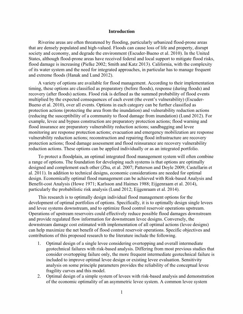
Introduction Riverine areas are often threatened by flooding, particularly urbanized flood-prone areas

that are densely populated and high-valued. Floods can cause loss of life and property, disrupt society and economy, and degrade the environment (Escuder-Bueno et al. 2010). In the United States, although flood-prone areas have received federal and local support to mitigate flood risks, flood damage is increasing (Pielke 2002; Smith and Katz 2013). California, with the complexity of its water system and the need for integrated approaches, in particular has to manage frequent and extreme floods (Hanak and Lund 2012).

A variety of options are available for flood management. According to their implementation timing, these options are classified as preparatory (before floods), response (during floods) and recovery (after floods) actions. Flood risk is defined as the summed probability of flood events multiplied by the expected consequences of each event (the event’s vulnerability) (Escuder-Bueno et al. 2010), over all events. Options in each category can be further classified as protection actions (protecting the area from the inundation) and vulnerability reduction actions (reducing the susceptibility of a community to flood damage from inundation) (Lund 2012). For example, levee and bypass construction are preparatory protection actions; flood warning and flood insurance are preparatory vulnerability reduction actions; sandbagging and levee monitoring are response protection actions; evacuation and emergency mobilization are response vulnerability reduction actions; reconstruction and repairing flood infrastructure are recovery protection actions; flood damage assessment and flood reinsurance are recovery vulnerability reduction actions. These options can be applied individually or as an integrated portfolio.

To protect a floodplain, an optimal integrated flood management system will often combine a range of options. The foundation for developing such systems is that options are optimally designed and complement each other (Zhu, et al. 2007; Patterson and Doyle 2009; Castellarin et al. 2011). In addition to technical designs, economic considerations are needed for optimal design. Economically optimal flood management can be achieved with Risk-based Analysis and Benefit-cost Analysis (Howe 1971; Karlsson and Haimes 1988; Eijgenraam et al. 2014), particularly the probabilistic risk analysis (Lund 2012; Eijgenraam et al. 2014).

This research is to optimally design individual flood management options for the development of optimal portfolios of options. Specifically, it is to optimally design single levees and levee systems downstream, and to optimize flood control reservoir operations upstream. Operations of upstream reservoirs could effectively reduce possible flood damages downstream and provide regulated flow information for downstream levee designs. Conversely, the downstream damage cost estimated with implementation of all optimal actions (levee designs) can help maximize the net benefit of flood control reservoir operations. Specific objectives and contributions of this proposed research to the literature include the following.

1. Optimal design of a single levee considering overtopping and overall intermediate geotechnical failures with risk-based analysis. Differing from most previous studies that consider overtopping failure only, the more frequent intermediate geotechnical failure is included to improve optimal levee design or existing levee evaluation. Sensitivity analysis on some principle parameters provides the reliability of the conceptual levee fragility curves and this model.

2. Optimal design of a simple system of levees with risk-based analysis and demonstration of the economic optimality of an asymmetric levee system. A common levee system

2

with two levees on opposite riverbanks on one river reach is optimally designed. Both symmetric and asymmetric levee systems are analyzed mathematically and theoretically, including overtopping and intermediate geotechnical failure modes, to demonstrate the economic optimality of better levee system designs.

3. Game theory is applied to analyze the decision making in a simple levee system where self-interested land owners on each river bank independently develop levee design strategies using risk-based optimization. The cooperative design game, single-shot non-cooperative Nash equilibrium, and the successive repeated reversible and irreversible non-cooperative games are examined. Comparing these different types of games can determine an appropriate level of compensation for the transferred flood risk to improve conditions for all parties.

4. Developing optimal flood hedging rules for a single reservoir through trading off current pre-release risk with future storm release risk given a flood forecast. Flood hedging pre-release is one way to improve control future large floods by increasing the frequency of small floods currently. The fundamental theoretical optimal condition for flood hedging pre-release requires that the current marginal damage cost from pre-releases equals the future expected damage cost from expected storms releases. Incorporating the economic water supply lost from pre-releases tends to reduce flood hedging pre-release, while blended hedging releases exist to include both water supply hedging and flood hedging.

Each of these topics will correspond to one chapter each in the doctoral dissertation and are discussed in detail below.

References Castellarin, A., Di Baldassarre, G., & Brath, A. (2011). Floodplain management strategies for

flood attenuation in the river Po. River Research and Applications, 27(8), 1037-1047. Eijgenraam, C., Kind, J., Bak, C., Brekelmans, R., den Hertog, D., Duits, M., ... & Kuijken, W.

(2014). Economically Efficient Standards to Protect the Netherlands Against Flooding. Interfaces, 44(1), 7-21.

Escuder-Bueno, I., Morales-Torres, A., & Perales-Momparler, S. (2010, March). Urban Flood Risk Characterization as a tool for planning and managing. In Workshop Alexandria, March.

Hanak, E., & Lund, J. R. (2012). Adapting California’s water management to climate change. Climatic Change, 111(1), 17-44.

Howe, W. (1971). Benefit‐Cost Analysis for Water System Planning (Vol. 2, pp. 1-144). American Geophysical Union.

Karlsson, P. O., & Haimes, Y. Y. (1988). Risk-based analysis of extreme events. Water Resources Research, 24(1), 9-20.

Lund, J. R. (2012). Flood management in California. Water, 4(1), 157-169. Pielke, R. A., Downton, M. W., & Miller, J. B. (2002). Flood damage in the United States, 1926-

2000: a reanalysis of National Weather Service estimates. Boulder, CO: University Corporation for Atmospheric Research.

Patterson, L. A., & Doyle, M. W. (2009). Assessing Effectiveness of National Flood Policy Through Spatiotemporal Monitoring of Socioeconomic Exposure1. JAWRA Journal of the American Water Resources Association, 45(1), 237-252.

3

Smith, A. B., & Katz, R. W. (2013). US billion-dollar weather and climate disasters: data sources, trends, accuracy and biases. Natural hazards, 67(2), 387-410.

Zhu, T., Lund, J. R., Jenkins, M. W., Marques, G. F., & Ritzema, R. S. (2007). Climate change, urbanization, and optimal long‐term floodplain protection. Water Resources Research, 43(6).

4

Chapter 1: Risk-Based Analysis for Optimal Single Levee Design

1.1 Summary

Traditional risk-based analysis for optimal levee design focuses primarily on overtopping failure. Although most levees fail before overtopping, few studies explicitly include intermediate geotechnical failures in flood risk analysis. This study develops a risk-based optimization model for levee designs given two simplified levee failure modes: overtopping and overall intermediate geotechnical failures. Overtopping failure is determined only by water level and levee height, while intermediate failure depends on geotechnical factors as well, represented by levee crown width according to conceptual levee fragility curves developed from professional judgment or analysis. The optimization minimizes the annual expected total cost, which sums expected annual damage and annualized construction cost. Applications of this optimization model in designing new levees or evaluating existing levees are demonstrated preliminarily for a levee on a small river with a low mean annual peak flow protecting agricultural land, and a major levee on a large river with a high mean annual peak flow protecting costly urban land. Sensitivity analysis on levee fragility curves is presented for overall optima under range of intermediate failure conditions.

1.2 Introduction

Levees partially protect land from flood damage by restraining water from entering the protected area. Even the best levees cannot guarantee protection, given levee failures under various conditions. Flood risk is the probability of failure multiplied by the consequences of failure summed over all events (Van Dantzig 1956; Eijgenraam et al. 2014; Arrow and Lind 1970). Levees can decrease, but not eliminate flood risk.

Risk-based analysis has been used to evaluate flood consequences since the 20th century. In 1960, the Netherlands, in its Delta Plan, first introduced return period (or exceedance frequency) for the optimal design water level to protect against flooding, based on a cost-benefit analysis to determine optimal return periods for dike rings in the Netherlands (Van Dantzig 1956; Van Der Most and Wehrung 2005; Eijgenraam et al. 2014; Kind 2014). The acceptable average return periods for the design of levees and dikes are stated in the Dutch Law, including four safety classes: 1250, 2000, 4000 and 10,000 years (Van Manen and Brinkhuis 2005). Flood risks considering probabilities and consequences have been established as a preferable basis for levee design and safety. Starting from 1992, the Technical Advisory Committee for Flood Defence initiated the development of a flood risk approach to more comprehensively calculate probabilities of flooding of dike ring areas. This method was applied to four illustrative case studies during its development (Technical Advisory Committee 2000) and has been widely accepted since then (Baan 2004; Klijn 2004; Jonkman 2008; Klijn 2008; Zhu and Lund 2009).

Most traditional risk analysis studies of levees only account for levee failure from overtopping, but levees often fail before overtopping due to intermediate geotechnical failures modes (Wolff 1997). Wolff (1997) modeled multiple individual failure modes and created a combined failure probability, assuming individual modes are independent. It summarizes that under-seepage and through-seepage are the two most common intermediate failure modes and may also trigger other failure modes such as erosion and slope stability. Although a few studies have analyzed the probability of intermediate levee failure as a function of water level (Technical

5

Advisory Committee 2000; Meehan and Benjasupattananan 2012), they are too simplistic for identification of levee’s geotechnical characteristics. This study, instead, includes explicitly the intermediate geotechnical failure mode in levee risk analysis based on synthetic levee performance curves. Through-seepage is chosen to represent general intermediate failure since under-seepage is more likely only if a levee has less permeability than its foundation.

As shorter levees are more likely to fail by overtopping and narrower levees are more likely to fail geotechnically (Wood 1977; Tung and Mays 1981a; Tung and Mays 1981b; Bogárdi and Máthé 1968), levee height and crown width are two significant parameters in levee design. Other design parameters include waterside slope angle and landside slope angle for a general levee with trapezoid cross section, as well as levee material, compaction and other factors. Levee design usually follows federal and local standards, such as the 100-year urban flood protection required by the Federal Emergency Management Agency (FEMA 2013), Bulletin 192-82 and PL 84-99 developed by California Depart of Water Resources (DWR) in particular for agricultural levees, and the 200-year flood protection by the 2012 Urban Levee Design Criteria (2012).

Section 1.3 of this chapter describes a risk-based optimization model for a single levee design, including model description, intermediate geotechnical levee failure and risk-based analysis incorporating both overtopping and intermediate geotechnical failure modes. Section 1.4 presents and discusses the illustrative applications of this model for a small rural levee and a large urban levee. Section 1.5 presents a sensitivity analysis on levee fragility curves that represent the intermediate failure probabilities, and analyzes the impacts from major economic parameters. Section 1.6 concludes with key findings.

1.3 Risk-based Optimization for a Single Levee

Typically, the optimization principle of levee risk analysis is to minimize all flood related costs, including costs of expected (residual) flood damages and those of flood protection (here levee construction) (Kind 2014). For this study, a model combining simple representations of hydraulic levee failure and economic cost is used to examine levee design parameters (height and width) by minimizing annual expected total costs, including expected annual damage cost and annualized construction cost. This examination shows the relative importance of considering intermediate geotechnical failure as part of studies on levee system risk analysis.

1.3.1 Model Description

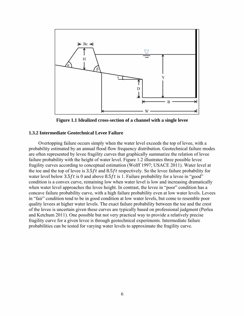
This study uses an idealized channel with a single levee on one side of a river reach and a high bank on the other side (that never fails) (Figure 1.1). is channel width, is the total channel and floodplain width till the toe of the levee, is channel depth, is water level, is the slope of the floodplain, is the levee landside slope, is the levee waterside slope, is levee height and is levee crown width. To simplify optimization of the levee considering both overtopping and intermediate geotechnical failure modes, levee height and crown width are assumed to be the two dominant variables, as surrogates for overtopping and geotechnical failure modes.

6

Figure 1.1 Idealized cross-section of a channel with a single levee

1.3.2 Intermediate Geotechnical Levee Failure

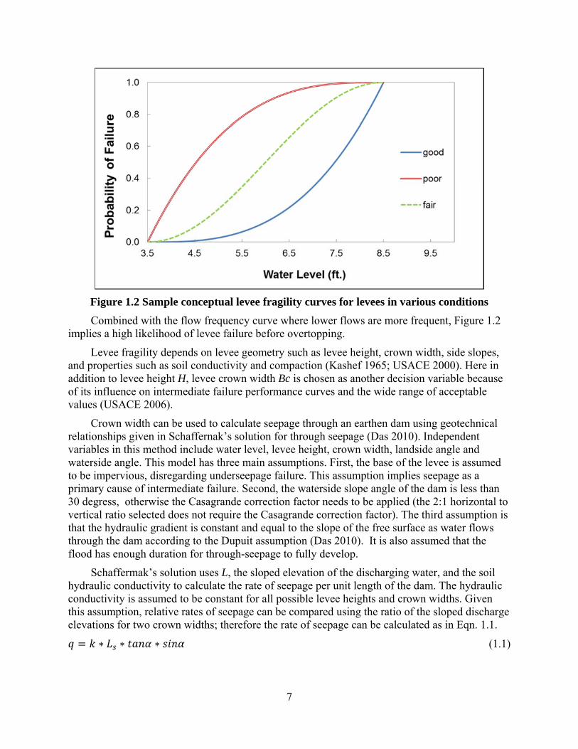
Overtopping failure occurs simply when the water level exceeds the top of levee, with a probability estimated by an annual flood flow frequency distribution. Geotechnical failure modes are often represented by levee fragility curves that graphically summarize the relation of levee failure probability with the height of water level. Figure 1.2 illustrates three possible levee fragility curves according to conceptual estimation (Wolff 1997; USACE 2011). Water level at the toe and the top of levee is 3.5 and 8.5 respectively. So the levee failure probability for water level below 3.5 is 0 and above 8.5 is 1. Failure probability for a levee in “good” condition is a convex curve, remaining low when water level is low and increasing dramatically when water level approaches the levee height. In contrast, the levee in “poor” condition has a concave failure probability curve, with a high failure probability even at low water levels. Levees in “fair” condition tend to be in good condition at low water levels, but come to resemble poor quality levees at higher water levels. The exact failure probability between the toe and the crest of the levee is uncertain given these curves are typically based on professional judgment (Perlea and Ketchum 2011). One possible but not very practical way to provide a relatively precise fragility curve for a given levee is through geotechnical experiments. Intermediate failure probabilities can be tested for varying water levels to approximate the fragility curve.

W

B

Bc

H

Y

D

τ

α β

7

Figure 1.2 Sample conceptual levee fragility curves for levees in various conditions

Combined with the flow frequency curve where lower flows are more frequent, Figure 1.2 implies a high likelihood of levee failure before overtopping.

Levee fragility depends on levee geometry such as levee height, crown width, side slopes, and properties such as soil conductivity and compaction (Kashef 1965; USACE 2000). Here in addition to levee height H, levee crown width Bc is chosen as another decision variable because of its influence on intermediate failure performance curves and the wide range of acceptable values (USACE 2006).

Crown width can be used to calculate seepage through an earthen dam using geotechnical relationships given in Schaffernak’s solution for through seepage (Das 2010). Independent variables in this method include water level, levee height, crown width, landside angle and waterside angle. This model has three main assumptions. First, the base of the levee is assumed to be impervious, disregarding underseepage failure. This assumption implies seepage as a primary cause of intermediate failure. Second, the waterside slope angle of the dam is less than 30 degress, otherwise the Casagrande correction factor needs to be applied (the 2:1 horizontal to vertical ratio selected does not require the Casagrande correction factor). The third assumption is that the hydraulic gradient is constant and equal to the slope of the free surface as water flows through the dam according to the Dupuit assumption (Das 2010). It is also assumed that the flood has enough duration for through-seepage to fully develop.

Schaffermak’s solution uses L, the sloped elevation of the discharging water, and the soil hydraulic conductivity to calculate the rate of seepage per unit length of the dam. The hydraulic conductivity is assumed to be constant for all possible levee heights and crown widths. Given this assumption, relative rates of seepage can be compared using the ratio of the sloped discharge elevations for two crown widths; therefore the rate of seepage can be calculated as in Eqn. 1.1.

∗ ∗ ∗ (1.1)

8

where is the rate of seepage per unit length of the levee, is the soil conductivity which is assumed constant in this study, is the angle of levee landside slope, and is the sloped elevation of the discharging water defined in Eqn. 1.2.

(1.2)

where is the water level, and is the horizontal distance between the landside toe of the levee and the effective seepage entrance as defined in Eqn. 1.3.

0.3 ∗ (1.3)

where is the angle of levee waterside slope, is levee height and is crown width.

The relative rates of seepage can be viewed as changes in the likelihood of levee through-seepage failure. At any given levee height, a wider levee would have a smaller sloped elevation

and a smaller seepage rate , therefore smaller exit velocity and through-seepage failure probability. So widening levee crown width decreases the likelihood of levee intermediate failure, which provides a basis for estimating the levee’s intermediate geotechnical failure.

To represent the relative probability of levee intermediate geotechnical failure, the minimum standard crown width is selected as base. Levee failure probability curves under different conditions for the minimum standard crown width are given based on the levee fragility curves. For numerical computation rather than theoretical analysis, this study uses the following mathematical expressions to explicitly represent levee fragility curves under good, fair and poor conditions respectively.

,

∗,

1 1 ,

(1.4)

where = probability of levee intermediate geotechnical failure and = height of the toe of levee. Mathematical formulas to represent levee fragility curves can be in other forms. For example, a simple linear function can approximate the intermediate failure of fair levees. This study is just illustrating an effective way to explicitly incorporate intermediate failure into levee risk-based analysis, not excluding alternative mathematical expressions options.

Levee failure probability for all other selected crown widths are normalized using the sloped elevation of the discharging water relative to that of this standard crown width, as a coefficient to adjust intermediate failure probability ( ).

,

, (1.5)

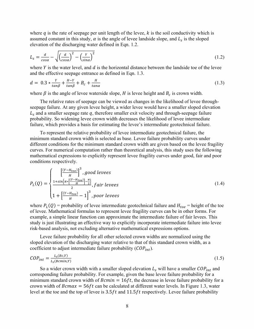
So a wider crown width with a smaller sloped elevation will have a smaller and corresponding failure probability. For example, given the base levee failure probability for a minimum standard crown width of 16 , the decrease in levee failure probability for a crown width of 56 can be calculated at different water levels. In Figure 1.3, water level at the toe and the top of levee is 3.5 and 11.5 respectively. Levee failure probability

9

curves have the same pattern for the same levee condition with either crown width. For the same water level and levee condition, failure probability for a crown width of 56 is less than at for the minimum standard crown width of 16 . The levee failure probability curves for a larger crown widths shift down and to the right from the original standard.

Figure 1.3 Levee failure probability curves for minimum and maximum levee crown widths in various levee conditions

The new levee fragility curves depend on both crown width and levee height, but continue to represent the professional judgment in the original levee fragility curves. Sensitivity analysis on this representation of levee fragility is presented later using an example of a rural levee.

1.3.3 Risk-based Optimization Model

This model assumes independence of overtopping and intermediate geotechnical failures for a given water level. It also assumes no hydraulic uncertainty affecting the relationship between water level and flow. Ignoring hydraulic uncertainty can compromise the accuracy of estimating expected damages, and should be avoided when adequate knowledge of the channel is available (Tung and Mays 1981b). Considering hydrologic uncertainties only, Eqn. 1.6 calculates the expected annual damage cost of the system for combined intermediate geotechnical and overtopping failures. The first term represents the expected damage from intermediate geotechnical failure when flow is below channel capacity, while the second term represents the expected damage from overtopping failure when flow exceeds the channel capacity.

∗ ∗ ∗ (1.6)

where = damage cost as a function of flow; = critical overtopping flow of the leveed channel; = probability density function of river flow; = probability of levee

10

intermediate geotechnical failure as a function of flow. The probability distribution of annual peak flood flow is assumed as a log-normal distribution. For a given channel geometry, Manning’s Equation is common for converting flow to water level (Wolff 1997).

If the damage cost per failure occurrence is constant and independent of flow (as in many deeply leveed systems), Eqn. 1.6 can be simplified to Eqn. 1.7.

∗ ∗ 1 (1.7)

where = constant flood damage cost; = cumulative density function of flow .

Therefore, the single levee design can be optimized by minimizing the annual expected total cost (TC), which is the sum of the expected annual damage cost (EAD) and annualized construction cost (ACC).

Min (1.8)

Annualized construction cost is based on levee volume and land area.

∗ ∗ ∗ ∗ (1.9)

where = real (inflation-adjusted) discount or interest rate; = number of useful years the levee will be repaid over; = a cost multiplier to cover engineering and construction administrative

costs; = unit construction cost per volume; ∗ ∗ ∗ ∗ is the

total volume of the levee along the entire length ( ) of the reach; ∗ is the cost for purchasing land to build the levee, with a unit land cost, , and the land area occupied by levee

base, ∗ ∗ . Land cost is an additional cost to represent the site-

specific expense of purchasing an acre land.

Physical constraints on this optimization model include upper and lower limits of crown width and levee height as well as non-negativity of all variables.

1.4 Model Applications

The developed risk-based optimization model is applied illustratively to a small rural Cosumnes River levee and a large urban Natomas levee in California. Hydraulic parameters and levee dimensions for model applications are formulated from previous studies (Tung and Mays 1981b), following design standards developed by DWR and the federal government, Bulletin 192-82 and PL 84-99 respectively. All the following economic values for annual expected total costs, annualized construction costs and expected annual damages costs are yearly costs.

1.4.1 Model Applications in A Small Rural Levee on Cosumnes River

The Cosumnes River has a median peak annual flow of 930 , a mean annual peak flow of 1300 , a land cost of $3000 per acre (0.066 $/ft2), and roughly $8 million damage cost if the area is flooded (USACE 2006).

Channel geometry and levee related parameters include: channel width is 200 ; total channel width including the floodplain is 250 ; channel depth is 3 ; longitudinal

11

slope of the channel and the floodplain section is 0.0005; Manning’s roughness for the channel section and floodplain is 0.05; floodplain slope is τ 0.01; levee landside slope and waterside slope are set as 1/4 and 1/2 respectively; total levee length is 2640 . Construction cost parameters are cost per unit levee material is

$10/ ; real discount rate is 0.05; useful life of the levee is 100 ; the cost multiplier for engineering and construction administrative costs is 1.3.

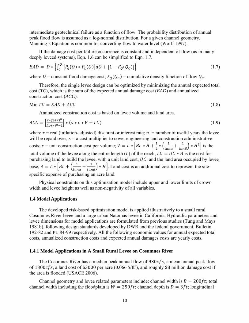
Using these site specific values and assuming the Cosumnes levee is under fair condition, the annualized construction cost, expected annual damage cost, and annual expected total cost are compared for a minimum levee crown width of 16 and a maximum of 56 in Figure 1.4, with 0.1 increment in varying levee height. Generally, annual expected total cost is dominated by the expected annual damage cost for shorter levees, and by the annualized construction cost for taller levees. The minimum of each total cost curve defines an optimum levee height for that crown width. In Figure 1.4, the optimal levee height for a minimum crown width of 16 is ∗ 6.7 , while the optimal levee height for a maximum crown width of 56 is ∗ 4.4 . The annual expected total cost for the minimum crown width exceeds that of the maximum crown width by $0.26 million/yr, as a results of a small decrease in annualized construction cost by $0.11 million/yr but a big increase in the expected annual damage cost by $0.37 million/yr.

Figure 1.4 Annual expected total costs, annualized construction costs and expected annual damage costs for different levee crown widths, assuming fair levee condition (rural levee)

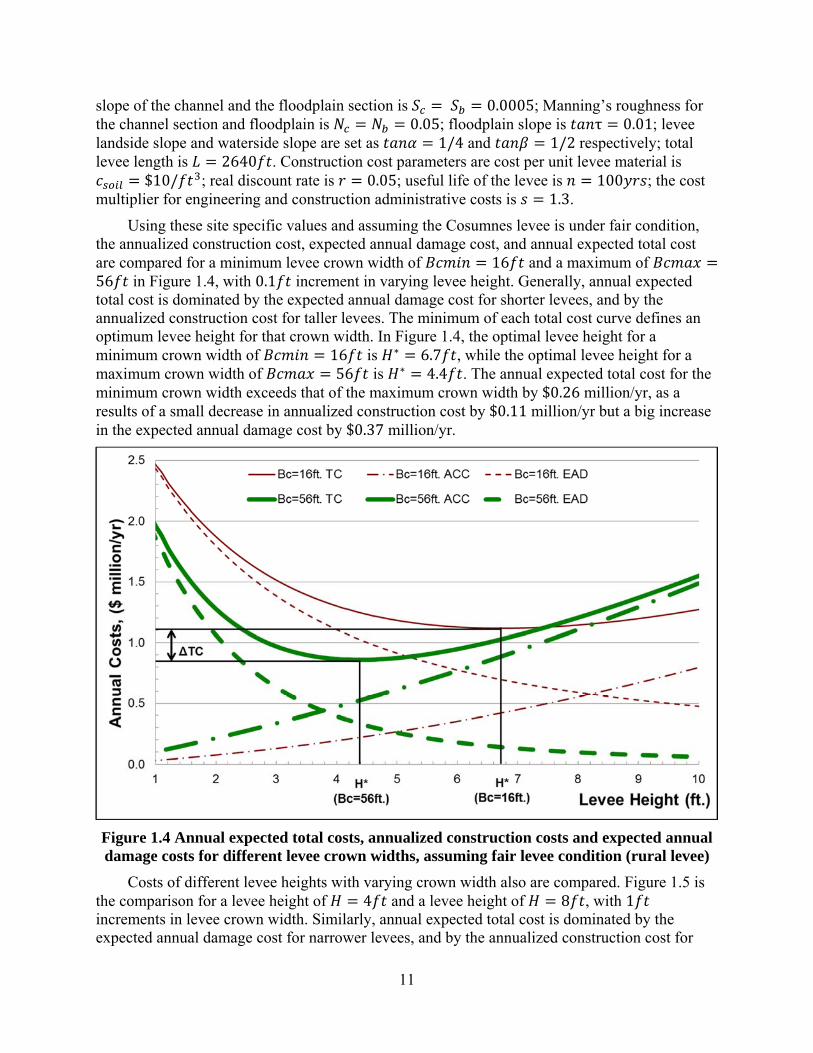
Costs of different levee heights with varying crown width also are compared. Figure 1.5 is the comparison for a levee height of 4 and a levee height of 8 , with 1 increments in levee crown width. Similarly, annual expected total cost is dominated by the expected annual damage cost for narrower levees, and by the annualized construction cost for

12

wider levees. With increases in levee height and/or crown width, the expected annual damage cost becomes extremely small due to the rapidly decreasing chance of overtopping and intermediate failure, and therefore total cost becomes dominated by construction cost. The minimum of each total cost curve defines an optimum levee crown width for that height. The optimal levee crown width for a levee height of 4 is ∗ 46 , while the optimal levee crown width for a levee height of 8 is ∗ 29 . The annual expected total cost for a levee height of 8 exceeds that of 4 by $0.14 million/yr, as a result of a big increase in annualized construction cost by $0.33 million/yr and a small decrease in the expected annual damage cost by $0.19 million/yr. Compared to the results from Figure 1.4, changes in levee height lead to greater changes in annualized construction cost than changes in levee crown width.

Figure 1.5 Annual expected total costs, annualized construction costs and expected annual damage costs for different levee heights, assuming fair levee condition (rural levee)

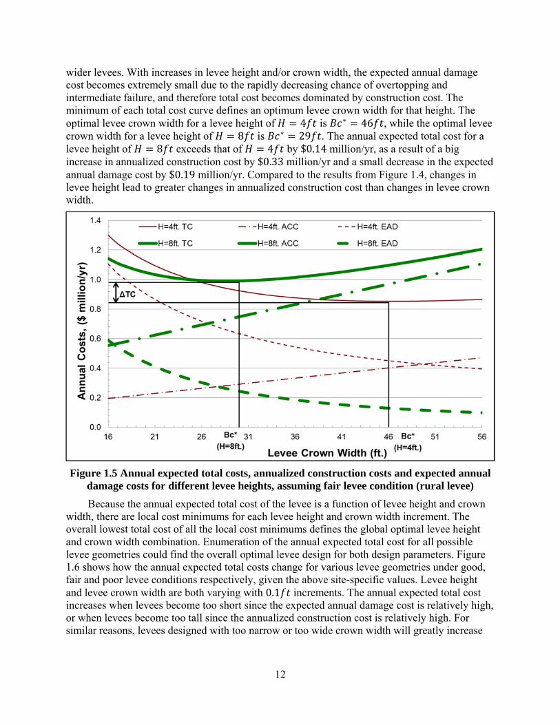
Because the annual expected total cost of the levee is a function of levee height and crown width, there are local cost minimums for each levee height and crown width increment. The overall lowest total cost of all the local cost minimums defines the global optimal levee height and crown width combination. Enumeration of the annual expected total cost for all possible levee geometries could find the overall optimal levee design for both design parameters. Figure 1.6 shows how the annual expected total costs change for various levee geometries under good, fair and poor levee conditions respectively, given the above site-specific values. Levee height and levee crown width are both varying with 0.1 increments. The annual expected total cost increases when levees become too short since the expected annual damage cost is relatively high, or when levees become too tall since the annualized construction cost is relatively high. For similar reasons, levees designed with too narrow or too wide crown width will greatly increase

13

the annual expected total cost. Minimum annual expected total cost occurs at a corresponding optimum combination of levee height and crown width.

Figure 1.6 Annual expected total costs for various levee geometries under good, fair and poor levee conditions (rural levee)

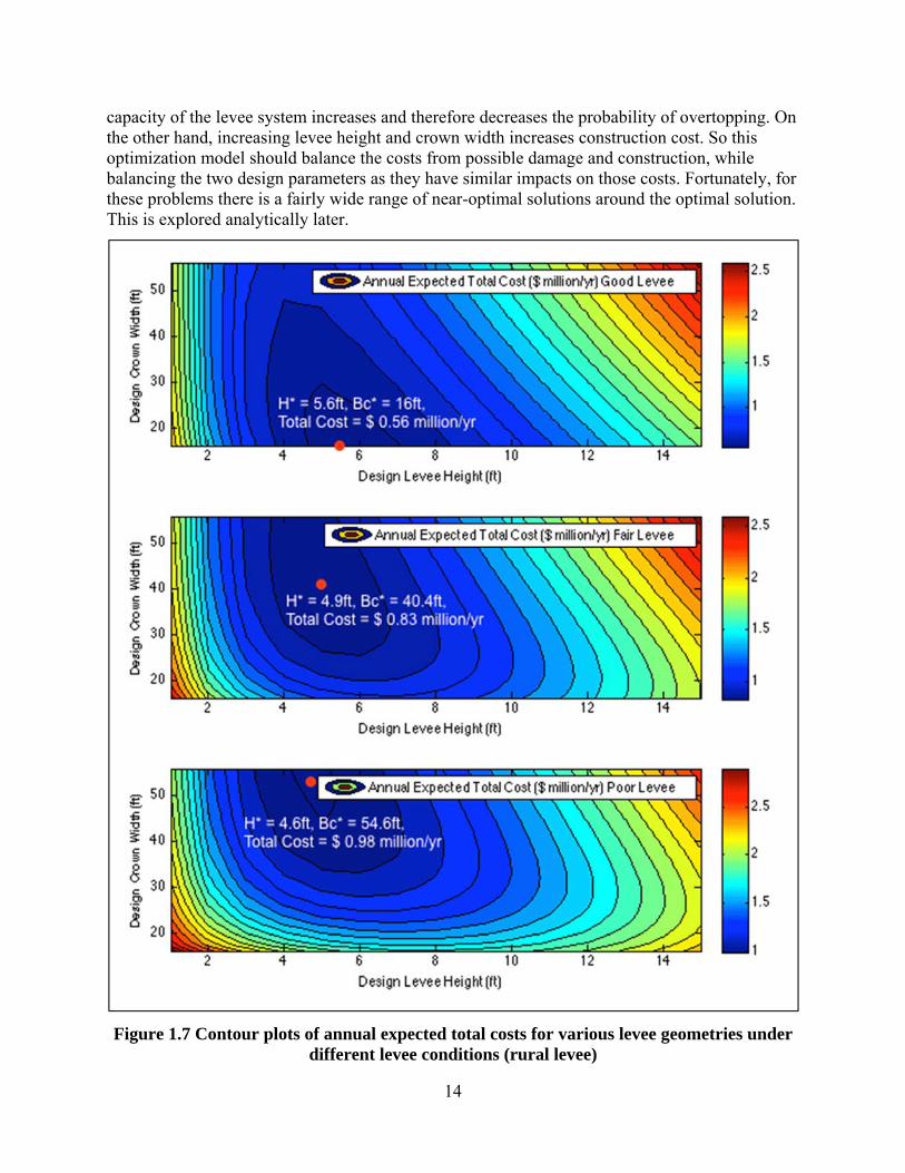
Another way to compare the optimum combination of levee height and crown width is by contour plots of all possible annual expected total costs (Figure 1.7). Contour intervals are $0.1 million/yr across plots for different levee conditions in Figure 1.7. The red dots on each contour plot indicate the optimal levee height and crown width. The contour plots reveal the trend that the optimum levee height decreases with increasing crown width, for a comparable total cost. As levee crown width increases, intermediate failure probability decreases and therefore decreases the first term of the expected annual damage equation. As the levee height increases, the

14

capacity of the levee system increases and therefore decreases the probability of overtopping. On the other hand, increasing levee height and crown width increases construction cost. So this optimization model should balance the costs from possible damage and construction, while balancing the two design parameters as they have similar impacts on those costs. Fortunately, for these problems there is a fairly wide range of near-optimal solutions around the optimal solution. This is explored analytically later.

Figure 1.7 Contour plots of annual expected total costs for various levee geometries under different levee conditions (rural levee)

15

Table 1.1 shows the optimal results for the three levee conditions and the trends of these results from good to poor levee conditions.

Table 1.1 Optimal results and comparison for different levee conditions (rural levee)

Optimal Results GOOD FAIR POOR Good to Poor Annual Expected Total Cost ($ million/yr) 0.56 0.83 0.98 Increasing Expected Annual Damage Cost ($ million/yr) 0.24 0.36 0.44 Increasing Annualized Construction Cost ($ million/yr) 0.32 0.47 0.54 Increasing Levee Height H (ft.) 5.6 4.9 4.6 Decreasing Levee Crown Width Bc (ft.) 16 40.4 54.6 Increasing Prob. Of Overtopping Failure 0.0089 0.0135 0.0162 Increasing Prob. Of Intermediate Failure 0.0211 0.0316 0.0386 Increasing Prob. Of Overall Failure 0.0300 0.0451 0.0548 Increasing Return Period (yrs) 112 74 62 Decreasing Return Period (yrs) (2ft freeboard) 287 215 202 Decreasing Return Period (yrs) (3ft freeboard) 396 319 287 Decreasing

Among the optimal values in Table 1.1, the optimal levee height and relevant return years

of the designed peak flow decrease from good to poor levee conditions, differing from the trends of others. Compared to big differences in optimum levee crown widths (16 40.454.6 ) of good, fair and poor conditions, the optimum levee height remains fairly constant around 5 (5.6 4.9 4.6 ). For the optimal combination, a levee with much narrower crown width has a slightly higher levee height, or a slightly higher levee has a much narrower crown width, and vice verse. This results from the levee geometry of the side slopes, specifically waterside slope 1/2 and landside slope 1/4. The annualized construction cost, which is a function of levee volume, is more sensitive to levee height than crown width; when a levee height increases by 1 , the base width increases by 6 t (1/ 1/ 6), which increases the horizontal distance of the seepage path and decreases seepage related failures. So under varying conditions, a bigger change in levee crown width can substitute for a smaller height change.

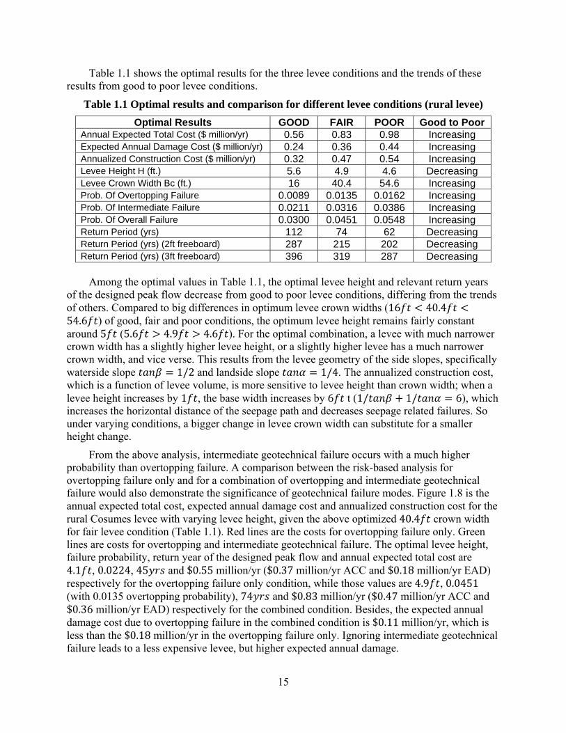
From the above analysis, intermediate geotechnical failure occurs with a much higher probability than overtopping failure. A comparison between the risk-based analysis for overtopping failure only and for a combination of overtopping and intermediate geotechnical failure would also demonstrate the significance of geotechnical failure modes. Figure 1.8 is the annual expected total cost, expected annual damage cost and annualized construction cost for the rural Cosumes levee with varying levee height, given the above optimized 40.4 crown width for fair levee condition (Table 1.1). Red lines are the costs for overtopping failure only. Green lines are costs for overtopping and intermediate geotechnical failure. The optimal levee height, failure probability, return year of the designed peak flow and annual expected total cost are 4.1 , 0.0224, 45 and $0.55 million/yr ($0.37 million/yr ACC and $0.18 million/yr EAD) respectively for the overtopping failure only condition, while those values are 4.9 , 0.0451 (with 0.0135 overtopping probability), 74 and $0.83 million/yr ($0.47 million/yr ACC and $0.36 million/yr EAD) respectively for the combined condition. Besides, the expected annual damage cost due to overtopping failure in the combined condition is $0.11 million/yr, which is less than the $0.18 million/yr in the overtopping failure only. Ignoring intermediate geotechnical failure leads to a less expensive levee, but higher expected annual damage.

16

Figure 1.8 Annual expected total costs, annualized construction costs and expected annual damage costs for overtopping failure only and a combination of overtopping and

intermediate geotechnical failure, assuming fair levee condition (rural levee)

In this example, land use cost ( ) has little impact on the optimal results, but the availability of land may constrain a levee’s base area ( ). The bottom width of the levee cross-section increases 6 per foot of additional height and increases 1 per foot of additional crown width. As the unit land cost ( ) increases by one increment, the optimal design will be a wider but slightly shorter levee since land use cost depends on the levee’s base area ( ∗ ). Where the optimum crown width is too large for a fixed land area, steeper landside slopes or a smaller crown width should be analyzed. In urban areas with high land prices, levees may be replaced with more expensive, but thinner flood walls. In contrast to the Cosumnes River surrounded primarily by agricultural land, next section looks at the Natomas levee on the Sacramento River that protects an urban area from a major river.

1.4.2 Model Applications in A Large Urban Natomas Levee on Sacramento River

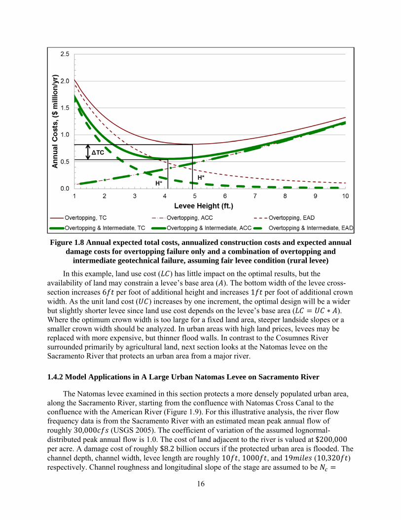
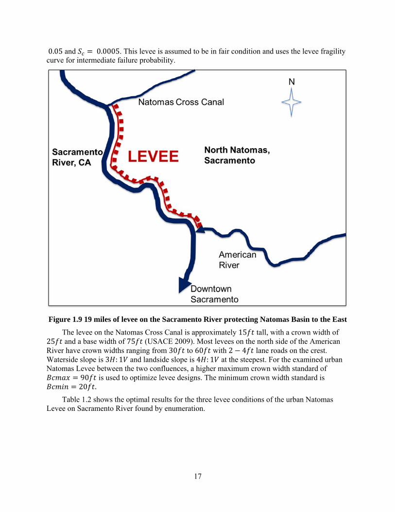
The Natomas levee examined in this section protects a more densely populated urban area, along the Sacramento River, starting from the confluence with Natomas Cross Canal to the confluence with the American River (Figure 1.9). For this illustrative analysis, the river flow frequency data is from the Sacramento River with an estimated mean peak annual flow of roughly 30,000 (USGS 2005). The coefficient of variation of the assumed lognormal-distributed peak annual flow is 1.0. The cost of land adjacent to the river is valued at $200,000 per acre. A damage cost of roughly $8.2 billion occurs if the protected urban area is flooded. The channel depth, channel width, levee length are roughly 10 , 1000 , and 19 (10,320 ) respectively. Channel roughness and longitudinal slope of the stage are assumed to be

17

0.05 and 0.0005. This levee is assumed to be in fair condition and uses the levee fragility curve for intermediate failure probability.

Figure 1.9 19 miles of levee on the Sacramento River protecting Natomas Basin to the East

The levee on the Natomas Cross Canal is approximately 15 tall, with a crown width of 25 and a base width of 75 (USACE 2009). Most levees on the north side of the American River have crown widths ranging from 30 to 60 with 2 4 lane roads on the crest. Waterside slope is 3 : 1 and landside slope is 4 : 1 at the steepest. For the examined urban Natomas Levee between the two confluences, a higher maximum crown width standard of

90 is used to optimize levee designs. The minimum crown width standard is 20 .

Table 1.2 shows the optimal results for the three levee conditions of the urban Natomas Levee on Sacramento River found by enumeration.

18

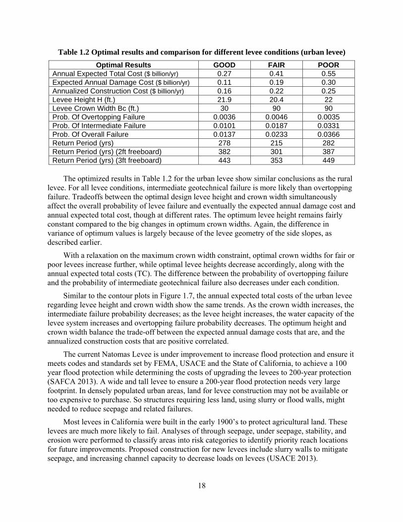
Table 1.2 Optimal results and comparison for different levee conditions (urban levee)

Optimal Results GOOD FAIR POOR Annual Expected Total Cost ($ billion/yr) 0.27 0.41 0.55 Expected Annual Damage Cost ($ billion/yr) 0.11 0.19 0.30 Annualized Construction Cost ($ billion/yr) 0.16 0.22 0.25 Levee Height H (ft.) 21.9 20.4 22 Levee Crown Width Bc (ft.) 30 90 90 Prob. Of Overtopping Failure 0.0036 0.0046 0.0035 Prob. Of Intermediate Failure 0.0101 0.0187 0.0331 Prob. Of Overall Failure 0.0137 0.0233 0.0366 Return Period (yrs) 278 215 282 Return Period (yrs) (2ft freeboard) 382 301 387 Return Period (yrs) (3ft freeboard) 443 353 449

The optimized results in Table 1.2 for the urban levee show similar conclusions as the rural

levee. For all levee conditions, intermediate geotechnical failure is more likely than overtopping failure. Tradeoffs between the optimal design levee height and crown width simultaneously affect the overall probability of levee failure and eventually the expected annual damage cost and annual expected total cost, though at different rates. The optimum levee height remains fairly constant compared to the big changes in optimum crown widths. Again, the difference in variance of optimum values is largely because of the levee geometry of the side slopes, as described earlier.

With a relaxation on the maximum crown width constraint, optimal crown widths for fair or poor levees increase further, while optimal levee heights decrease accordingly, along with the annual expected total costs (TC). The difference between the probability of overtopping failure and the probability of intermediate geotechnical failure also decreases under each condition.

Similar to the contour plots in Figure 1.7, the annual expected total costs of the urban levee regarding levee height and crown width show the same trends. As the crown width increases, the intermediate failure probability decreases; as the levee height increases, the water capacity of the levee system increases and overtopping failure probability decreases. The optimum height and crown width balance the trade-off between the expected annual damage costs that are, and the annualized construction costs that are positive correlated.

The current Natomas Levee is under improvement to increase flood protection and ensure it meets codes and standards set by FEMA, USACE and the State of California, to achieve a 100 year flood protection while determining the costs of upgrading the levees to 200-year protection (SAFCA 2013). A wide and tall levee to ensure a 200-year flood protection needs very large footprint. In densely populated urban areas, land for levee construction may not be available or too expensive to purchase. So structures requiring less land, using slurry or flood walls, might needed to reduce seepage and related failures.

Most levees in California were built in the early 1900’s to protect agricultural land. These levees are much more likely to fail. Analyses of through seepage, under seepage, stability, and erosion were performed to classify areas into risk categories to identify priority reach locations for future improvements. Proposed construction for new levees include slurry walls to mitigate seepage, and increasing channel capacity to decrease loads on levees (USACE 2013).

19

1.5 Sensitivity Analysis

Several factors could affect this optimization model, including the conceptual levee fragility curves and values of various economic parameters. Sensitivity analysis is applied to these major factors to understand their impacts.

1.5.1 Impacts from Levee Fragility Curves

The levee fragility curves serve as the foundation to include intermediate geotechnical failure in optimal levee design for this study. Derivation and representation of the levee fragility curves are important in this risk-based optimization model. The proposed method of addressing intermediate geotechnical failure probability combines professional judgment in the original levee fragility curves with a more physics-based way of representing effectiveness of wider crown widths. Sensitivity analysis on the derived levee fragility curves, and their mathematical expressions, is discussed with examples of the rural Cosumnes levee.

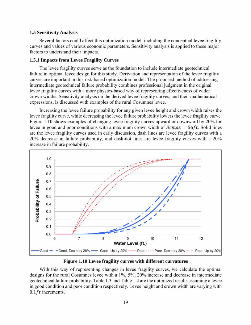
Increasing the levee failure probability for any given levee height and crown width raises the levee fragility curve, while decreasing the levee failure probability lowers the levee fragility curve. Figure 1.10 shows examples of changing levee fragility curves upward or downward by 20% for levee in good and poor conditions with a maximum crown width of 56 . Solid lines are the levee fragility curves used in early discussion, dash lines are levee fragility curves with a 20% decrease in failure probability, and dash-dot lines are levee fragility curves with a 20% increase in failure probability.

Figure 1.10 Levee fragility curves with different curvatures

With this way of representing changes in levee fragility curves, we calculate the optimal designs for the rural Cosumnes levee with a 1%, 5%, 20% increase and decrease in intermediate geotechnical failure probability. Table 1.3 and Table 1.4 are the optimized results assuming a levee in good condition and poor condition respectively. Levee height and crown width are varying with 0.1 increments.

20

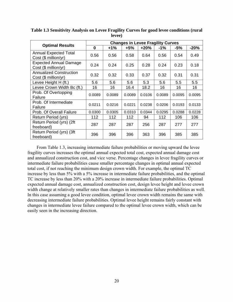
Table 1.3 Sensitivity Analysis on Levee Fragility Curves for good levee conditions (rural levee)

Optimal Results Changes in Levee Fragility Curves

0 +1% +5% +20% -1% -5% -20% Annual Expected Total Cost ($ million/yr)

0.56 0.56 0.58 0.64 0.56 0.54 0.49

Expected Annual Damage Cost ($ million/yr)

0.24 0.24 0.25 0.28 0.24 0.23 0.18

Annualized Construction Cost ($ million/yr)

0.32 0.32 0.33 0.37 0.32 0.31 0.31

Levee Height H (ft.) 5.6 5.6 5.6 5.3 5.6 5.5 5.5 Levee Crown Width Bc (ft.) 16 16 16.4 18.2 16 16 16 Prob. Of Overtopping Failure

0.0089 0.0089 0.0089 0.0106 0.0089 0.0095 0.0095

Prob. Of Intermediate Failure

0.0211 0.0216 0.0221 0.0238 0.0206 0.0193 0.0133

Prob. Of Overall Failure 0.0300 0.0305 0.0310 0.0344 0.0295 0.0288 0.0228 Return Period (yrs) 112 112 112 94 112 106 106 Return Period (yrs) (2ft freeboard)

287 287 287 256 287 277 277

Return Period (yrs) (3ft freeboard)

396 396 396 363 396 385 385

From Table 1.3, increasing intermediate failure probabilities or moving upward the levee

fragility curves increases the optimal annual expected total cost, expected annual damage cost and annualized construction cost, and vice verse. Percentage changes in levee fragility curves or intermediate failure probabilities cause smaller percentage changes in optimal annual expected total cost, if not reaching the minimum design crown width. For example, the optimal TC increase by less than 5% with a 5% increase in intermediate failure probabilities, and the optimal TC increase by less than 20% with a 20% increase in intermediate failure probabilities. Optimal expected annual damage cost, annualized construction cost, design levee height and levee crown width change at relatively smaller rates than changes in intermediate failure probabilities as well. In this case assuming a good levee condition, optimal levee crown width remains the same with decreasing intermediate failure probabilities. Optimal levee height remains fairly constant with changes in intermediate levee failure compared to the optimal levee crown width, which can be easily seen in the increasing direction.

21

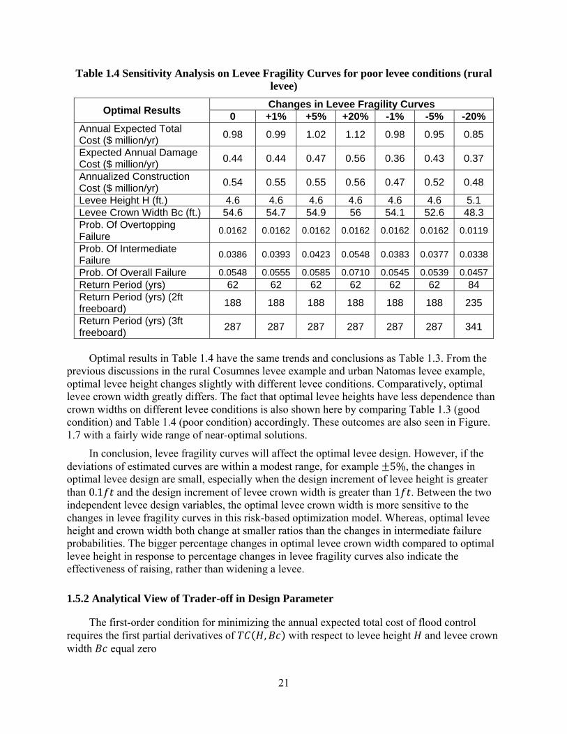
Table 1.4 Sensitivity Analysis on Levee Fragility Curves for poor levee conditions (rural levee)

Optimal Results Changes in Levee Fragility Curves

0 +1% +5% +20% -1% -5% -20% Annual Expected Total Cost ($ million/yr)

0.98 0.99 1.02 1.12 0.98 0.95 0.85

Expected Annual Damage Cost ($ million/yr)

0.44 0.44 0.47 0.56 0.36 0.43 0.37

Annualized Construction Cost ($ million/yr)

0.54 0.55 0.55 0.56 0.47 0.52 0.48

Levee Height H (ft.) 4.6 4.6 4.6 4.6 4.6 4.6 5.1 Levee Crown Width Bc (ft.) 54.6 54.7 54.9 56 54.1 52.6 48.3 Prob. Of Overtopping Failure

0.0162 0.0162 0.0162 0.0162 0.0162 0.0162 0.0119

Prob. Of Intermediate Failure

0.0386 0.0393 0.0423 0.0548 0.0383 0.0377 0.0338

Prob. Of Overall Failure 0.0548 0.0555 0.0585 0.0710 0.0545 0.0539 0.0457 Return Period (yrs) 62 62 62 62 62 62 84 Return Period (yrs) (2ft freeboard)

188 188 188 188 188 188 235

Return Period (yrs) (3ft freeboard)

287 287 287 287 287 287 341

Optimal results in Table 1.4 have the same trends and conclusions as Table 1.3. From the

previous discussions in the rural Cosumnes levee example and urban Natomas levee example, optimal levee height changes slightly with different levee conditions. Comparatively, optimal levee crown width greatly differs. The fact that optimal levee heights have less dependence than crown widths on different levee conditions is also shown here by comparing Table 1.3 (good condition) and Table 1.4 (poor condition) accordingly. These outcomes are also seen in Figure. 1.7 with a fairly wide range of near-optimal solutions.

In conclusion, levee fragility curves will affect the optimal levee design. However, if the deviations of estimated curves are within a modest range, for example 5%, the changes in optimal levee design are small, especially when the design increment of levee height is greater than 0.1 and the design increment of levee crown width is greater than 1 . Between the two independent levee design variables, the optimal levee crown width is more sensitive to the changes in levee fragility curves in this risk-based optimization model. Whereas, optimal levee height and crown width both change at smaller ratios than the changes in intermediate failure probabilities. The bigger percentage changes in optimal levee crown width compared to optimal levee height in response to percentage changes in levee fragility curves also indicate the effectiveness of raising, rather than widening a levee.

1.5.2 Analytical View of Trader-off in Design Parameter

The first-order condition for minimizing the annual expected total cost of flood control requires the first partial derivatives of , with respect to levee height and levee crown width equal zero

22

∗∗

∗ ∗ ∗ ∗0

(1.10)

∗∗

∗ ∗ ∗ ∗0 (1.11)

Assuming uniform flow in the river channel, the overtopping capacity is determined solely by river cross-section geometry, which is levee height in this case. Energy slope and channel roughness are not supposed to be affected by levee modification. Therefore, from Eqn. 1.10 and 1.11,

∗ ∗

(1.12)

The above equation holds for the optimal levee height and optimal levee crown width. Other than the enumeration method discussed previously for solving this optimization model, the optimal levee height and crown width can also be found by numerically solving the two first-order conditions simultaneously and verifying that a global minimum is attained.

In the above equation, value of flood damage cost , unit construction cost , economic discount rate , and land use cost do not affect the optimal trade-off between levee height and crown width. Thus, changes in these economic values do not affect the economic optimal ratio of substitution between levee height and crown width, though may affect the values of the optimal design.

1.6 Conclusion

This study presents a quantitative risk-based analysis for optimal single levee design including overtopping and intermediate geotechnical failure modes to estimate the optimal levee height and crown width. By using the geotechnical relationships given in Schaffernak’s solution for through seepage, levee crown width is added as an independent decision variable that primarily determines the intermediate geotechnical failure probability. In this way, the conceptual levee fragility curves, which largely represent professional judgment, are quantitatively adjusted to include both levee height and levee crown width and represent both overtopping and intermediate geotechnical failure modes.

In this risk-based optimal levee design, levee height determines overtopping probability while levee height and crown width together determine the likelihood of intermediate geotechnical failure. The optimal levee height and crown width are found by minimizing the annual expected total cost, which is the sum of expected annual damage and annualized construction cost. Other than optimal design of a levee, this approach could also help evaluate the current condition of existing levees.

This risk-based optimization model is demonstrated for a rural levee on a small river and an unban levee on a major river in California. Increasing levee height reduces overtopping failure, while increasing crown width decreases intermediate geotechnical failure in both large and more frequent smaller floods. As the probability of intermediate geotechnical failure can be much larger than that of overtopping failure, intermediate failure should be included in analyses. Furthermore, the optimal crown width of a levee in good condition can be significantly smaller

23

than the optimum crown width of a levee in poor condition, while the optimal levee height remains fairly constant for all levee conditions.

Sensitivity analysis shows the impact of levee fragility curves. Changes to other levee design parameters cause fewer design and cost changes than changing the overall levee fragility curves representing intermediate failure probabilities. The optimal levee crown width is more sensitive than the optimal levee height in response to the changes in levee fragility curves. The optimal levee height remains fairly constant with different levee fragility curves shapes. These indicate the effectiveness of levee height in determining the optimal levee design or resisting changes in other parameters.

With the assumptions and simplifications used in this risk-based analysis, further study should address limitations, such as by including more realistic descriptions of channel geometry, damage cost function, levee fragility curves and failure modes. The effect of levee length also should be analyzed in future work since a longer levee should be more likely to fail.

1.7 References

Arrow, K. J., & Lind, R. C. (1970). Uncertainty and the Evaluation of Public Investment Decisions. American Economic Review, 60(3), 364-78.

Baan, P. J., & Klijn, F. (2004). Flood risk perception and implications for flood risk management in the Netherlands. International Journal of River Basin Management, 2(2), 113-122.

Bogárdi, I., & Máthé, Z. (1968). Determination of the degree of protection offered by flood levees and the economic improvement thereof. National Water Authority, Department for Flood Control and River Training.

Das, B. M. (2010), Seeepage, Principles of Geotechnical Engineering, Edition 7, 198-225. Eijgenraam, C., Kind, J., Bak, C., Brekelmans, R., den Hertog, D., Duits, M., ... & Kuijken, W.

(2014). Economically Efficient Standards to Protect the Netherlands Against Flooding. Interfaces, 44(1), 7-21.

FEMA (2013), Levees: Information for Cooperating Technical Partners and Engineers. Jonkman, S. N., Kok, M., & Vrijling, J. K. (2008). Flood risk assessment in the Netherlands: A

case study for dike ring South Holland. Risk Analysis, 28(5), 1357-1374. Kashef, A. A. I. (1965). Seepage through earth dams. Journal of Geophysical Research, 70(24),

6121-6128. Kind, J. M. (2014). Economically efficient flood protection standards for the Netherlands.

Journal of Flood Risk Management, 7(2), 103-117. Klijn, F., van Buuren, M., & van Rooij, S. A. (2004). Flood-risk management strategies for an

uncertain future: living with Rhine river floods in the Netherlands?. AMBIO: A Journal of the Human Environment, 33(3), 141-147.

Klijn, F., Samuels, P., & Van Os, A. (2008). Towards flood risk management in the EU: State of affairs with examples from various European countries. International Journal of River Basin Management, 6(4), 307-321.

Meehan, C. L., & Benjasupattananan, S. (2012). An analytical approach for levee underseepage analysis. Journal of Hydrology, 470, 201-211.

Perlea, M., & Ketchum, E. (2011). Impact of Non-Analytical Factors in Geotechnical Risk Assessment of Levees. Reston, VA: ASCE copyright Proceedings of Georisk 2011, June 26. 28, 2011, Atlanta, Georgia| d 20110000.

SACFA. (2013), Natomas Levee Improvement Program.

24

Technical Advisory Committee for Flood Defence in the Netherlands. (2000). From Probability of Exceedance to Probability of Flooding.

Tung, Y. K., & Mays, L. W. (1981a). Risk models for flood levee design. Water Resources Research, 17(4), 833-841.

Tung, Y. K., & Mays, L. W. (1981b). Optimal risk‐based design of flood levee systems. Water Resources Research, 17(4), 843-852.

Urban Levee Design Criteria (2012), FloodSafe California. USACE (2000), EM 1110-2-1913, Engineering and Design - Design and Construction of Levees. USACE (2006), TL 1110-2-561, Reliability Analysis and Risk Assessment for Seepage and

Slope Stability Failure Modes for Embankment Dams. USACE (2009), Final Environmental Impact Statement on the Natomas Levee Improvement

Program: Phase 3 Landside Improvement Project. USACE (2011), Cranford Levee reliability project for flood risk management Rahway, Cranford,

NJ. USACE (2013), Missions: Civil Works: Levee Safety Program: Levee Inspection. USGS (2005) “Introduction to the Sacramento River Basin”. U.S. Geological Survey Circular

1215. U.S. Geological Survey. 2005-09-01. Retrieved 2010-08-31. Van Dantzig, D. (1956). Economic decision problems for flood prevention. Econometrica:

Journal of the Econometric Society, 276-287. Van Der Most, H., & Wehrung, M. (2005). Dealing with uncertainty in flood risk assessment of

dike rings in the Netherlands. Natural Hazards, 36(1-2), 191-206. Van Manen, S. E., & Brinkhuis, M. (2005). Quantitative flood risk assessment for Polders.

Reliability engineering & system safety, 90(2), 229-237. Wolff, T. F. (1997). Geotechnical reliability of levees. In Proc of a Hydrology and Hydraulics

Workshop on Risk-Based Analysis for Flood Damage Reduction Studies, USACE, Hydrologic Engineering Center.

Wood, E. (1977). An analysis of flood levee reliability. Water Resources Research, 13(3), 665-671.

Zhu, T., & Lund, J. R. (2009). Up or Out?—Economic-Engineering Theory of Flood Levee Height and Setback. Journal of Water Resources Planning and Management, 135(2), 90-95.

25

Chapter 2: Risk-Based Analysis for Optimal Simple Levee System Design

2.1 Summary

Risk-based analysis has been applied to optimal levee design for purpose of economic efficiency, including the previous study of single levee design considering both overtopping and the more frequent intermediate geotechnical failures. Normally along a river, each river side has a levee that together acting as a levee system. The levee failure risk of levee systems should be analyzed to minimize overall economic costs. This study examines a common simple levee system with two levees on opposite riverbanks, with either symmetric or asymmetric levee geometry, allowing flood risk transfer across the river. Risk-based analysis is used to demonstrate the economic optimality of an asymmetric levee system mathematically and analytically, for overtopping failure and overall intermediate geotechnical failure. As individual costs generally increase, compensation for transferred flood risk should be negotiated and guaranteed to improve conditions for all parties. This one reach levee system could be further extended to include upstream and downstream reaches.

2.2 Introduction

Levees can protect flood prone areas by increasing channel capacity for retaining flood flow within the leveed channel rather than entering the protected area. However, levees could fail by the well-known overtopping failure and the more frequently observed intermediate geotechnical failure, even at a low probability. As risk is defined as the failure probability multiplied by the consequences of failure, levees can decrease but cannot eliminate the likelihood of flooding (Hashimoto et al. 1982).

Risk-based analysis has long been applied to optimal levee design, for example the basic risk models for flood levee design which systematically analyzed the various hydrologic and hydraulic uncertainties (Tung and Mays1981), and previous study of single levee design considering both overtopping and intermediate geotechnical failures (Chapter 1). A taller and wider levee can decrease the failure probability thus to reduce the expected damage cost, but it also increases the construction cost. The optimal design should be the one minimizing total cost including both damage and construction costs. For a levee system along a river with two levees on opposite riverbanks, which is a usual case, the overall cost on two sides from expected damage and construction should be optimized with risk-based analysis.

Different levee system design can change how flood risk is distributed, either symmetric levee system that two levees are exactly the same, or asymmetric levee system that one levee is more likely to fail. Croghan (2013) discussed in her thesis the concepts of economic flood risk transformation and transference among floodplain users. She found that total flood risk can be reduced from transferring risk from the high cost urban floodplain to the low-valued rural floodplain of a river. One may predict that such asymmetric levee system allowing flood risk transfer across the river can also reduce the total cost containing construction as well. To provide a foundation for this prediction, the overall economic optimality of such asymmetric levee system should be proved mathematically and analytically

This chapter proceeds as follows. Section 2.3 describes the Risk-based optimization model for a simple levee system design, including model description, risk-based analysis for overtopping failure, intermediate geotechnical levee failure and a combination of both failure

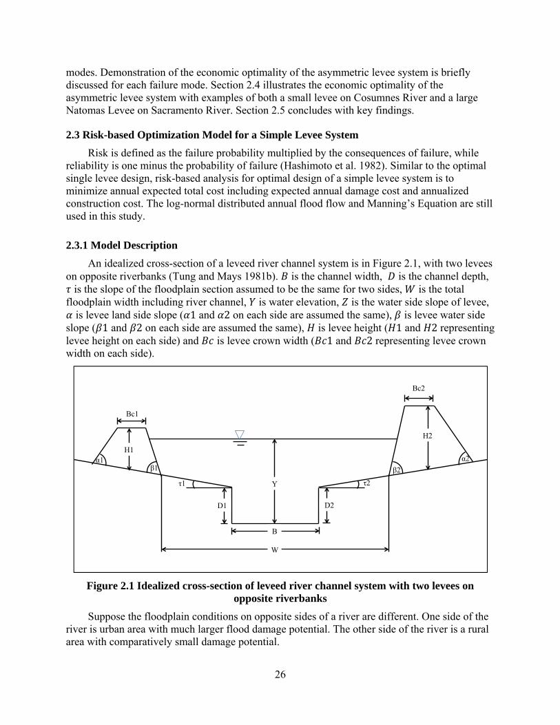
26

modes. Demonstration of the economic optimality of the asymmetric levee system is briefly discussed for each failure mode. Section 2.4 illustrates the economic optimality of the asymmetric levee system with examples of both a small levee on Cosumnes River and a large Natomas Levee on Sacramento River. Section 2.5 concludes with key findings.

2.3 Risk-based Optimization Model for a Simple Levee System

Risk is defined as the failure probability multiplied by the consequences of failure, while reliability is one minus the probability of failure (Hashimoto et al. 1982). Similar to the optimal single levee design, risk-based analysis for optimal design of a simple levee system is to minimize annual expected total cost including expected annual damage cost and annualized construction cost. The log-normal distributed annual flood flow and Manning’s Equation are still used in this study.

2.3.1 Model Description

An idealized cross-section of a leveed river channel system is in Figure 2.1, with two levees on opposite riverbanks (Tung and Mays 1981b). is the channel width, is the channel depth, is the slope of the floodplain section assumed to be the same for two sides, is the total

floodplain width including river channel, is water elevation, is the water side slope of levee, is levee land side slope ( 1 and 2 on each side are assumed the same), is levee water side

slope ( 1 and 2 on each side are assumed the same), is levee height ( 1 and 2 representing levee height on each side) and is levee crown width ( 1 and 2 representing levee crown width on each side).

Figure 2.1 Idealized cross-section of leveed river channel system with two levees on opposite riverbanks

Suppose the floodplain conditions on opposite sides of a river are different. One side of the river is urban area with much larger flood damage potential. The other side of the river is a rural area with comparatively small damage potential.

W

B

Bc1

H1

Y

D1

τ1

α1 β1

D2

τ2

Bc2

H2

β2

α2

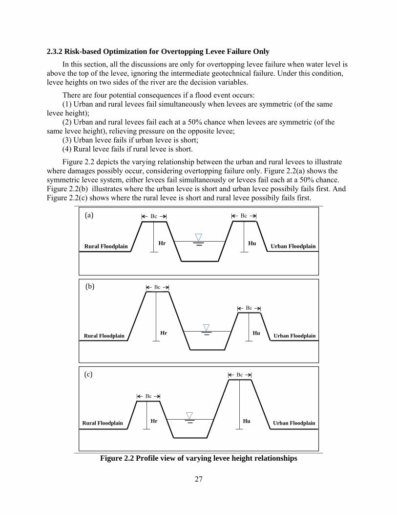
27

2.3.2 Risk-based Optimization for Overtopping Levee Failure Only

In this section, all the discussions are only for overtopping levee failure when water level is above the top of the levee, ignoring the intermediate geotechnical failure. Under this condition, levee heights on two sides of the river are the decision variables.

There are four potential consequences if a flood event occurs: (1) Urban and rural levees fail simultaneously when levees are symmetric (of the same

levee height); (2) Urban and rural levees fail each at a 50% chance when levees are symmetric (of the

same levee height), relieving pressure on the opposite levee; (3) Urban levee fails if urban levee is short; (4) Rural levee fails if rural levee is short.

Figure 2.2 depicts the varying relationship between the urban and rural levees to illustrate where damages possibly occur, considering overtopping failure only. Figure 2.2(a) shows the symmetric levee system, either levees fail simultaneously or levees fail each at a 50% chance. Figure 2.2(b) illustrates where the urban levee is short and urban levee possibily fails first. And Figure 2.2(c) shows where the rural levee is short and rural levee possibily fails first.

Figure 2.2 Profile view of varying levee height relationships

Rural Floodplain Urban Floodplain Hr Hu

Bc Bc

Rural Floodplain Urban Floodplain Hr Hu

Bc

Bc

Rural Floodplain Urban Floodplain Hr Hu

Bc

Bc

(a)

(b)

(c)

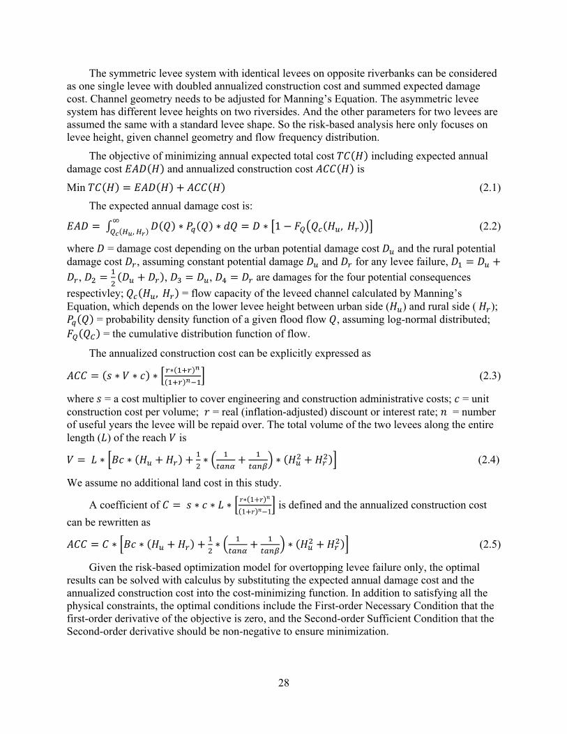
28

The symmetric levee system with identical levees on opposite riverbanks can be considered as one single levee with doubled annualized construction cost and summed expected damage cost. Channel geometry needs to be adjusted for Manning’s Equation. The asymmetric levee system has different levee heights on two riversides. And the other parameters for two levees are assumed the same with a standard levee shape. So the risk-based analysis here only focuses on levee height, given channel geometry and flow frequency distribution.

The objective of minimizing annual expected total cost including expected annual damage cost and annualized construction cost is

Min (2.1)

The expected annual damage cost is:

∗ ∗, ∗ 1 , (2.2)

where = damage cost depending on the urban potential damage cost and the rural potential damage cost , assuming constant potential damage and for any levee failure,

, , , are damages for the four potential consequences

respectivley; , = flow capacity of the leveed channel calculated by Manning’s Equation, which depends on the lower levee height between urban side ( ) and rural side ( );

= probability density function of a given flood flow , assuming log-normal distributed; = the cumulative distribution function of flow.

The annualized construction cost can be explicitly expressed as

∗ ∗ ∗ ∗ (2.3)

where = a cost multiplier to cover engineering and construction administrative costs; = unit construction cost per volume; = real (inflation-adjusted) discount or interest rate; = number of useful years the levee will be repaid over. The total volume of the two levees along the entire length ( ) of the reach is

∗ ∗ ∗ ∗ (2.4)

We assume no additional land cost in this study.

A coefficient of ∗ ∗ ∗ ∗ 1

1 1 is defined and the annualized construction cost

can be rewritten as

∗ ∗ ∗ ∗ (2.5)

Given the risk-based optimization model for overtopping levee failure only, the optimal results can be solved with calculus by substituting the expected annual damage cost and the annualized construction cost into the cost-minimizing function. In addition to satisfying all the physical constraints, the optimal conditions include the First-order Necessary Condition that the first-order derivative of the objective is zero, and the Second-order Sufficient Condition that the Second-order derivative should be non-negative to ensure minimization.

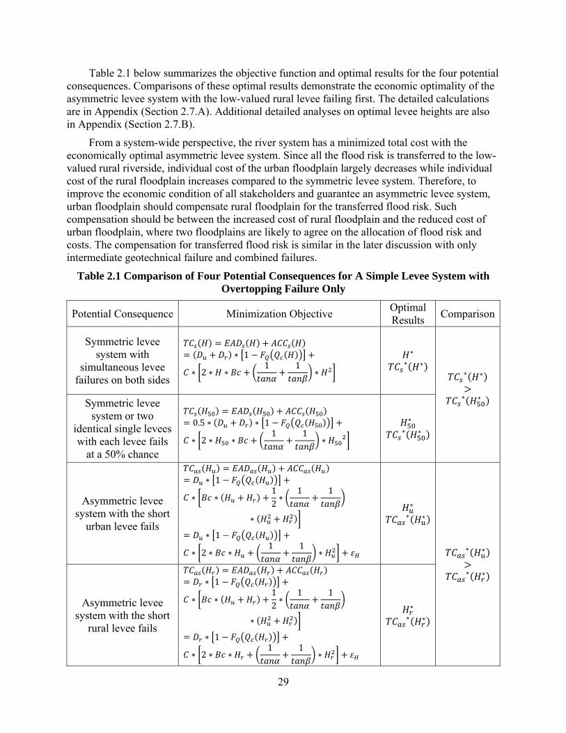
29

Table 2.1 below summarizes the objective function and optimal results for the four potential consequences. Comparisons of these optimal results demonstrate the economic optimality of the asymmetric levee system with the low-valued rural levee failing first. The detailed calculations are in Appendix (Section 2.7.A). Additional detailed analyses on optimal levee heights are also in Appendix (Section 2.7.B).

From a system-wide perspective, the river system has a minimized total cost with the economically optimal asymmetric levee system. Since all the flood risk is transferred to the low-valued rural riverside, individual cost of the urban floodplain largely decreases while individual cost of the rural floodplain increases compared to the symmetric levee system. Therefore, to improve the economic condition of all stakeholders and guarantee an asymmetric levee system, urban floodplain should compensate rural floodplain for the transferred flood risk. Such compensation should be between the increased cost of rural floodplain and the reduced cost of urban floodplain, where two floodplains are likely to agree on the allocation of flood risk and costs. The compensation for transferred flood risk is similar in the later discussion with only intermediate geotechnical failure and combined failures.

Table 2.1 Comparison of Four Potential Consequences for A Simple Levee System with Overtopping Failure Only

Potential Consequence Minimization Objective Optimal Results

Comparison

Symmetric levee system with

simultaneous levee failures on both sides

∗ 1

∗ 2 ∗ ∗1 1

∗

∗ ∗ ∗

∗ ∗

∗ ∗

Symmetric levee system or two

identical single levees with each levee fails

at a 50% chance

0.5 ∗ ∗ 1

∗ 2 ∗ ∗1 1

∗

∗ ∗ ∗

Asymmetric levee system with the short

urban levee fails

∗ 1

∗ ∗12∗

1 1

∗

∗ 1

∗ 2 ∗ ∗1 1

∗

∗ ∗ ∗

∗ ∗

∗ ∗

Asymmetric levee system with the short

rural levee fails

∗ 1

∗ ∗12∗

1 1

∗

∗ 1

∗ 2 ∗ ∗1 1

∗

∗ ∗ ∗

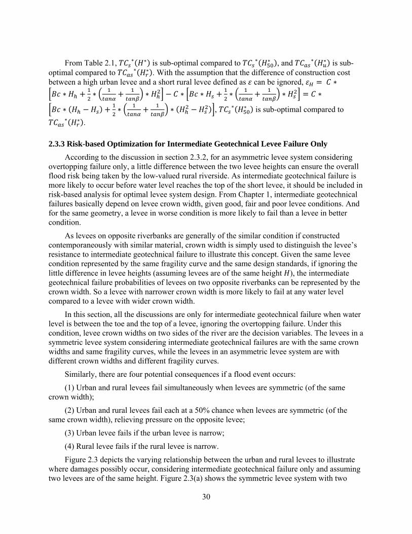
30

From Table 2.1, ∗ ∗ is sub-optimal compared to ∗ ∗ , and ∗ ∗ is sub-

optimal compared to ∗ ∗ . With the assumption that the difference of construction cost between a high urban levee and a short rural levee defined as can be ignored,

∗

∗ ∗ ∗ ∗ ∗ ∗ ∗ ∗

∗ ∗ ∗ , ∗ ∗ is sub-optimal compared to ∗ ∗ .

2.3.3 Risk-based Optimization for Intermediate Geotechnical Levee Failure Only

According to the discussion in section 2.3.2, for an asymmetric levee system considering overtopping failure only, a little difference between the two levee heights can ensure the overall flood risk being taken by the low-valued rural riverside. As intermediate geotechnical failure is more likely to occur before water level reaches the top of the short levee, it should be included in risk-based analysis for optimal levee system design. From Chapter 1, intermediate geotechnical failures basically depend on levee crown width, given good, fair and poor levee conditions. And for the same geometry, a levee in worse condition is more likely to fail than a levee in better condition.

As levees on opposite riverbanks are generally of the similar condition if constructed contemporaneously with similar material, crown width is simply used to distinguish the levee’s resistance to intermediate geotechnical failure to illustrate this concept. Given the same levee condition represented by the same fragility curve and the same design standards, if ignoring the little difference in levee heights (assuming levees are of the same height ), the intermediate geotechnical failure probabilities of levees on two opposite riverbanks can be represented by the crown width. So a levee with narrower crown width is more likely to fail at any water level compared to a levee with wider crown width.

In this section, all the discussions are only for intermediate geotechnical failure when water level is between the toe and the top of a levee, ignoring the overtopping failure. Under this condition, levee crown widths on two sides of the river are the decision variables. The levees in a symmetric levee system considering intermediate geotechnical failures are with the same crown widths and same fragility curves, while the levees in an asymmetric levee system are with different crown widths and different fragility curves.

Similarly, there are four potential consequences if a flood event occurs:

(1) Urban and rural levees fail simultaneously when levees are symmetric (of the same crown width);

(2) Urban and rural levees fail each at a 50% chance when levees are symmetric (of the same crown width), relieving pressure on the opposite levee;

(3) Urban levee fails if the urban levee is narrow;

(4) Rural levee fails if the rural levee is narrow.

Figure 2.3 depicts the varying relationship between the urban and rural levees to illustrate where damages possibly occur, considering intermediate geotechnical failure only and assuming two levees are of the same height. Figure 2.3(a) shows the symmetric levee system with two

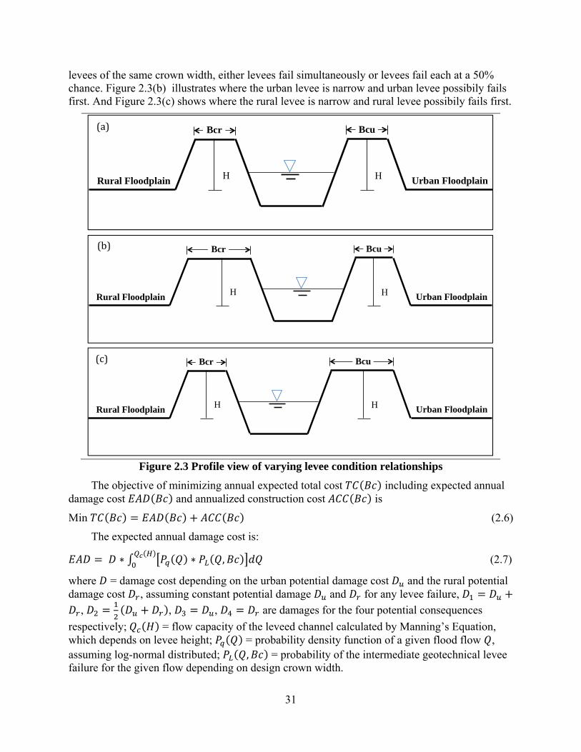
31

levees of the same crown width, either levees fail simultaneously or levees fail each at a 50% chance. Figure 2.3(b) illustrates where the urban levee is narrow and urban levee possibily fails first. And Figure 2.3(c) shows where the rural levee is narrow and rural levee possibily fails first.

Figure 2.3 Profile view of varying levee condition relationships

The objective of minimizing annual expected total cost including expected annual damage cost and annualized construction cost is

Min (2.6)

The expected annual damage cost is:

∗ ∗ , (2.7)

where = damage cost depending on the urban potential damage cost and the rural potential damage cost , assuming constant potential damage and for any levee failure,

, , , are damages for the four potential consequences

respectively; = flow capacity of the leveed channel calculated by Manning’s Equation, which depends on levee height; = probability density function of a given flood flow , assuming log-normal distributed; , = probability of the intermediate geotechnical levee failure for the given flow depending on design crown width.

Rural Floodplain Urban Floodplain H H

Bcr Bcu

Rural Floodplain Urban Floodplain H H

Bcr Bcu

Rural Floodplain Urban Floodplain H H

Bcr Bcu

(a)

(b)

(c)

32

With the simplifying assumptions above, the intermediate geotechnical levee failure probability of a narrower levee , should always be greater than that of a wider levee

, for any water level (any flow ). is the crown width of a narrower levee, is the crown width of a wider levee and .

The annualized construction cost can be explicitly expressed as

∗ ∗ ∗ ∗ (2.8)

∗ ∗ ∗ (2.9)

With the defined coefficient ∗ ∗ ∗ ∗ 1

1 1, the annualized construction cost can

be rewritten as

∗ ∗ ∗ (2.10)

Similarly, given the risk-based optimization model for intermediate geotechnical levee failure only, the optimal results can be solved with calculus by substituting the expected annual damage cost and the annualized construction cost into the cost-minimizing function. The optimal conditions would include the First-order Necessary Condition and the Second-order Sufficient Condition except for satisfying all the physical constraints,

Table 2.2 below summarizes the objective function and optimal results for the four potential consequences. Comparisons of these optimal results demonstrate the economic optimality of the asymmetric levee system with the low-valued rural levee failing first. The detailed calculations are in Appendix (Section 2.7.C).

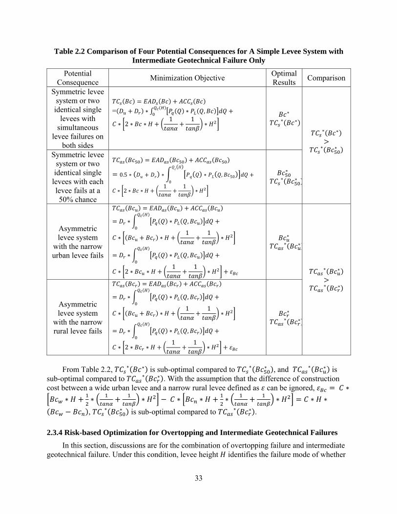
33

Table 2.2 Comparison of Four Potential Consequences for A Simple Levee System with Intermediate Geotechnical Failure Only

Potential Consequence

Minimization Objective Optimal Results

Comparison

Symmetric levee system or two identical single

levees with simultaneous

levee failures on both sides

= ∗ ∗ ,

∗ 2 ∗ ∗1 1

∗

∗ ∗ ∗

∗ ∗

∗ ∗ Symmetric levee

system or two identical single

levees with each levee fails at a 50% chance

0.5 ∗ ∗ ∗ , 500

∗ 2 ∗ ∗1 1

∗

∗ ∗ ∗

Asymmetric levee system

with the narrow urban levee fails

∗ ∗ ,

∗ ∗1 1

∗

∗ ∗ ,

∗ 2 ∗ ∗1 1

∗

∗ ∗ ∗

∗ ∗

∗ ∗

Asymmetric levee system

with the narrow rural levee fails

∗ ∗ ,

∗ ∗1 1

∗

∗ ∗ ,

∗ 2 ∗ ∗1 1

∗

∗ ∗ ∗

From Table 2.2, ∗ ∗ is sub-optimal compared to ∗ ∗ , and ∗ ∗ is

sub-optimal compared to ∗ ∗ . With the assumption that the difference of construction cost between a wide urban levee and a narrow rural levee defined as can be ignored,

∗

∗ ∗ ∗

∗ ∗ ∗ ∗ ∗ ∗

, ∗ ∗ is sub-optimal compared to ∗ ∗ .

2.3.4 Risk-based Optimization for Overtopping and Intermediate Geotechnical Failures

In this section, discussions are for the combination of overtopping failure and intermediate geotechnical failure. Under this condition, levee height identifies the failure mode of whether

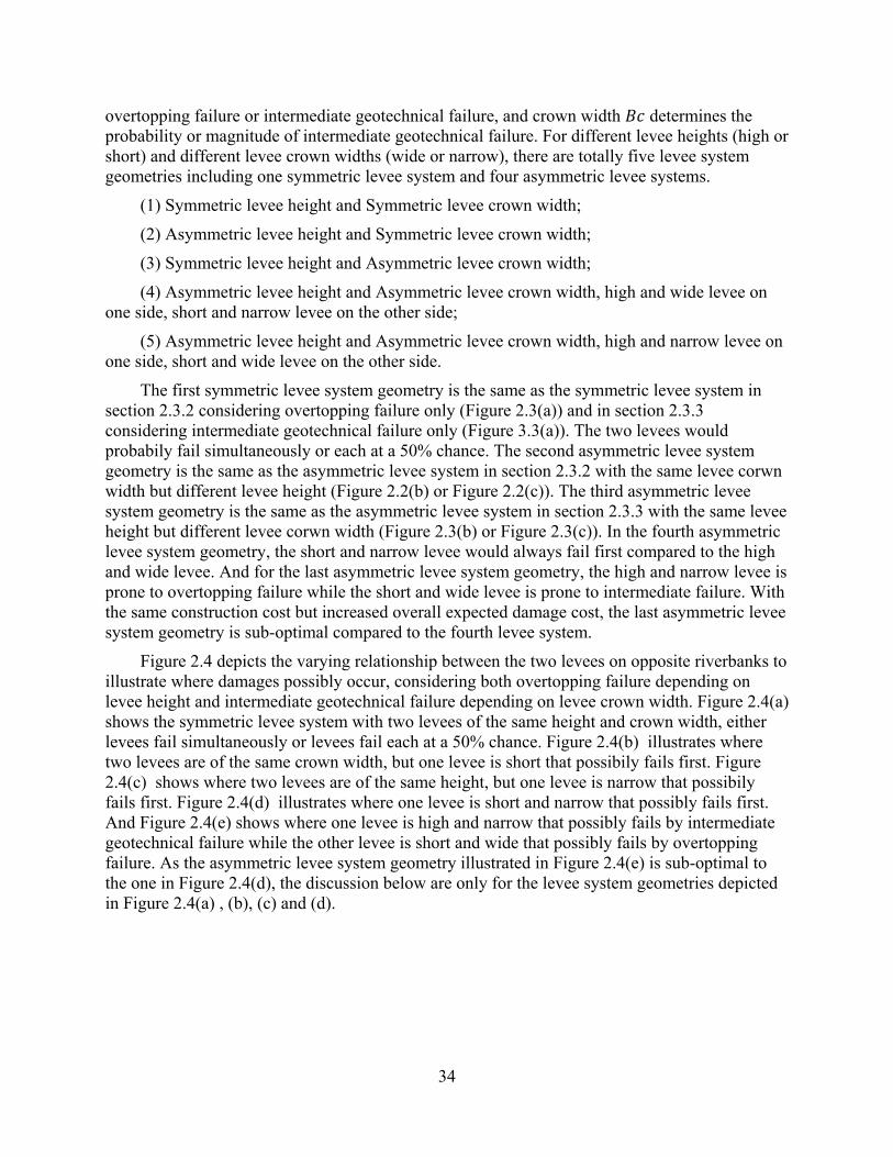
34

overtopping failure or intermediate geotechnical failure, and crown width determines the probability or magnitude of intermediate geotechnical failure. For different levee heights (high or short) and different levee crown widths (wide or narrow), there are totally five levee system geometries including one symmetric levee system and four asymmetric levee systems.

(1) Symmetric levee height and Symmetric levee crown width;

(2) Asymmetric levee height and Symmetric levee crown width;

(3) Symmetric levee height and Asymmetric levee crown width;

(4) Asymmetric levee height and Asymmetric levee crown width, high and wide levee on one side, short and narrow levee on the other side;

(5) Asymmetric levee height and Asymmetric levee crown width, high and narrow levee on one side, short and wide levee on the other side.

The first symmetric levee system geometry is the same as the symmetric levee system in section 2.3.2 considering overtopping failure only (Figure 2.3(a)) and in section 2.3.3 considering intermediate geotechnical failure only (Figure 3.3(a)). The two levees would probabily fail simultaneously or each at a 50% chance. The second asymmetric levee system geometry is the same as the asymmetric levee system in section 2.3.2 with the same levee corwn width but different levee height (Figure 2.2(b) or Figure 2.2(c)). The third asymmetric levee system geometry is the same as the asymmetric levee system in section 2.3.3 with the same levee height but different levee corwn width (Figure 2.3(b) or Figure 2.3(c)). In the fourth asymmetric levee system geometry, the short and narrow levee would always fail first compared to the high and wide levee. And for the last asymmetric levee system geometry, the high and narrow levee is prone to overtopping failure while the short and wide levee is prone to intermediate failure. With the same construction cost but increased overall expected damage cost, the last asymmetric levee system geometry is sub-optimal compared to the fourth levee system.

Figure 2.4 depicts the varying relationship between the two levees on opposite riverbanks to illustrate where damages possibly occur, considering both overtopping failure depending on levee height and intermediate geotechnical failure depending on levee crown width. Figure 2.4(a) shows the symmetric levee system with two levees of the same height and crown width, either levees fail simultaneously or levees fail each at a 50% chance. Figure 2.4(b) illustrates where two levees are of the same crown width, but one levee is short that possibily fails first. Figure 2.4(c) shows where two levees are of the same height, but one levee is narrow that possibily fails first. Figure 2.4(d) illustrates where one levee is short and narrow that possibly fails first. And Figure 2.4(e) shows where one levee is high and narrow that possibly fails by intermediate geotechnical failure while the other levee is short and wide that possibly fails by overtopping failure. As the asymmetric levee system geometry illustrated in Figure 2.4(e) is sub-optimal to the one in Figure 2.4(d), the discussion below are only for the levee system geometries depicted in Figure 2.4(a) , (b), (c) and (d).

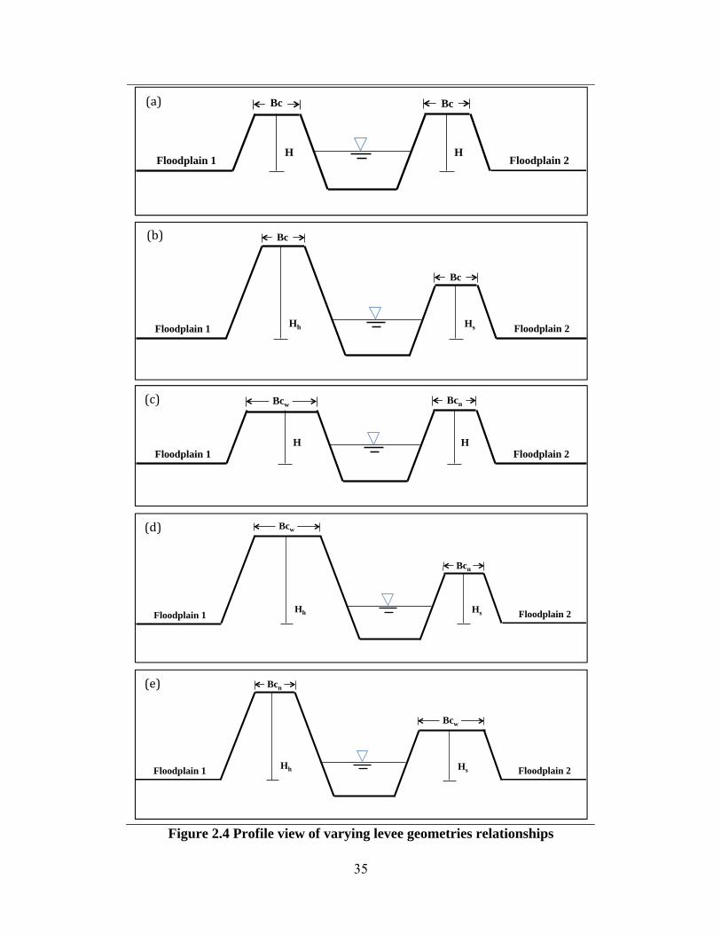
35

Figure 2.4 Profile view of varying levee geometries relationships

Floodplain 1 Floodplain 2

Bc Bc

H H

Floodplain 1 Floodplain 2 Hh Hs

Bc

Bc

H H Floodplain 1 Floodplain 2

Bcw Bcn

Floodplain 1 Floodplain 2 Hh Hs

Bcn

Bcw

Floodplain 1 Floodplain 2 Hh Hs

Bcn

Bcw

(a)

(b)

(e)

(c)

(d)

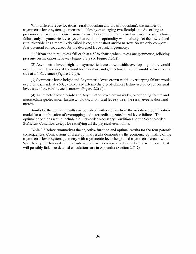
36

With different levee locations (rural floodplain and urban floodplain), the number of asymmetric levee system geometries doubles by exchanging two floodplains. According to previous discussions and conclusions for overtopping failure only and intermediate geotechnical failure only, asymmetric levee system at economic optimality would always let the low-valued rural riverside has a more likely failed levee, either short and/or narrow. So we only compare four potential consequences for the designed levee system geometry.

(1) Urban and rural levees fail each at a 50% chance when levees are symmetric, relieving pressure on the opposite levee (Figure 2.2(a) or Figure 2.3(a));

(2) Asymmetric levee height and symmetric levee crown width, overtopping failure would occur on rural levee side if the rural levee is short and geotechnical failure would occur on each side at a 50% chance (Figure 2.2(c));

(3) Symmetric levee height and Asymmetric levee crown width, overtopping failure would occur on each side at a 50% chance and intermediate geotechnical failure would occur on rural levee side if the rural levee is narrow (Figure 2.3(c));

(4) Asymmetric levee height and Asymmetric levee crown width, overtopping failure and intermediate geotechnical failure would occur on rural levee side if the rural levee is short and narrow.

Similarly, the optimal results can be solved with calculus from the risk-based optimization model for a combination of overtopping and intermediate geotechnical levee failures. The optimal conditions would include the First-order Necessary Condition and the Second-order Sufficient Condition except for satisfying all the physical constraints,

Table 2.3 below summarizes the objective function and optimal results for the four potential consequences. Comparisons of these optimal results demonstrate the economic optimality of the asymmetric levee system geometry with asymmetric levee height and asymmetric crown width. Specifically, the low-valued rural side would have a comparatively short and narrow levee that will possibly fail. The detailed calculations are in Appendix (Section 2.7.D).

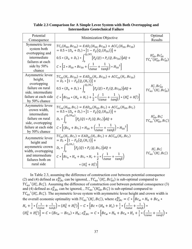
37

Table 2.3 Comparison for A Simple Levee System with Both Overtopping and Intermediate Geotechnical Failure

Potential Consequence

Minimization Objective Optimal Results

Symmetric levee system both

overtopping and intermediate

failures at each side by 50%

chance

, , , 0.5 ∗ ∗ 1

0.5 ∗ ∗ ∗ ,

∗ 2 ∗ ∗1 1

∗

∗ , ∗ ∗ ∗ , ∗

Asymmetric levee height,

overtopping failure on rural

side, intermediate failure at each side

by 50% chance

, , , ∗ 1

0.5 ∗ ∗ ∗ ,

∗ ∗12∗

1 1∗

∗, ∗ ∗ ∗, ∗

Asymmetric levee crown width, intermediate

failure on rural side, overtopping

failure at each side by 50% chance

, , , 0.5 ∗ ∗ 1

∗ ∗ ,

∗ ∗1 1

∗

∗ , ∗ ∗ ∗ , ∗

Asymmetric levee height and

asymmetric crown width, overtopping and intermediate failures both on

rural side

, , , ∗ 1

∗ ∗ ,

∗ ∗ ∗12∗

1 1

∗

∗, ∗ ∗ ∗, ∗

In Table 2.3, assuming the difference of construction cost between potential consequence

(2) and (4) defined as , can be ignored, , ∗ ∗, ∗ is sub-optimal compared to ∗ ∗, ∗ . Assuming the difference of construction cost between potential consequence (3)

and (4) defined as , can be ignored, , ∗ ∗ , ∗ is sub-optimal compared to ∗ ∗, ∗ . The asymmetric levee system with asymmetric levee height and crown width is

the overall economic optimality with ∗ ∗, ∗ , where , ∗ ∗ ∗

∗ ∗ ∗ ∗ ∗ ∗

∗ ∗ ; , ∗ ∗ ∗ ∗ ∗

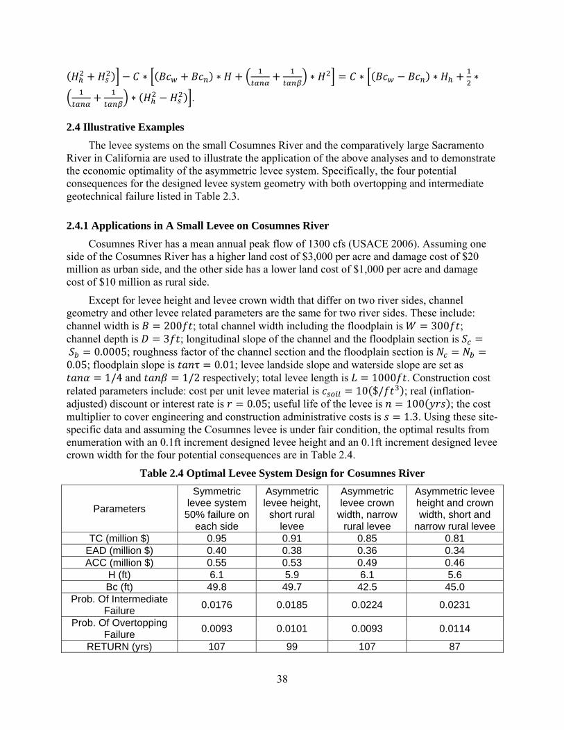
38

∗ ∗ ∗ ∗ ∗ ∗

∗ .

2.4 Illustrative Examples

The levee systems on the small Cosumnes River and the comparatively large Sacramento River in California are used to illustrate the application of the above analyses and to demonstrate the economic optimality of the asymmetric levee system. Specifically, the four potential consequences for the designed levee system geometry with both overtopping and intermediate geotechnical failure listed in Table 2.3.

2.4.1 Applications in A Small Levee on Cosumnes River

Cosumnes River has a mean annual peak flow of 1300 cfs (USACE 2006). Assuming one side of the Cosumnes River has a higher land cost of $3,000 per acre and damage cost of $20 million as urban side, and the other side has a lower land cost of $1,000 per acre and damage cost of $10 million as rural side.

Except for levee height and levee crown width that differ on two river sides, channel geometry and other levee related parameters are the same for two river sides. These include: channel width is 200 ; total channel width including the floodplain is 300 ; channel depth is 3 ; longitudinal slope of the channel and the floodplain section is 0.0005; roughness factor of the channel section and the floodplain section is 0.05; floodplain slope is τ 0.01; levee landside slope and waterside slope are set as

1/4 and 1/2 respectively; total levee length is 1000 . Construction cost related parameters include: cost per unit levee material is 10 $/ ; real (inflation-adjusted) discount or interest rate is 0.05; useful life of the levee is 100 ; the cost multiplier to cover engineering and construction administrative costs is 1.3. Using these site-specific data and assuming the Cosumnes levee is under fair condition, the optimal results from enumeration with an 0.1ft increment designed levee height and an 0.1ft increment designed levee crown width for the four potential consequences are in Table 2.4.

Table 2.4 Optimal Levee System Design for Cosumnes River

Parameters

Symmetric levee system

50% failure on each side

Asymmetric levee height,

short rural levee

Asymmetric levee crown

width, narrow rural levee

Asymmetric levee height and crown width, short and

narrow rural levee TC (million $) 0.95 0.91 0.85 0.81

EAD (million $) 0.40 0.38 0.36 0.34 ACC (million $) 0.55 0.53 0.49 0.46

H (ft) 6.1 5.9 6.1 5.6 Bc (ft) 49.8 49.7 42.5 45.0

Prob. Of Intermediate Failure

0.0176 0.0185 0.0224 0.0231

Prob. Of Overtopping Failure

0.0093 0.0101 0.0093 0.0114

RETURN (yrs) 107 99 107 87

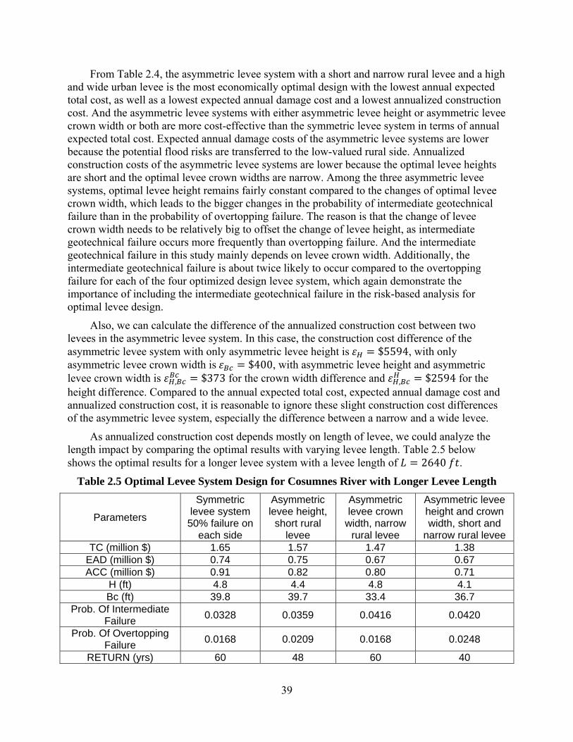
39

From Table 2.4, the asymmetric levee system with a short and narrow rural levee and a high and wide urban levee is the most economically optimal design with the lowest annual expected total cost, as well as a lowest expected annual damage cost and a lowest annualized construction cost. And the asymmetric levee systems with either asymmetric levee height or asymmetric levee crown width or both are more cost-effective than the symmetric levee system in terms of annual expected total cost. Expected annual damage costs of the asymmetric levee systems are lower because the potential flood risks are transferred to the low-valued rural side. Annualized construction costs of the asymmetric levee systems are lower because the optimal levee heights are short and the optimal levee crown widths are narrow. Among the three asymmetric levee systems, optimal levee height remains fairly constant compared to the changes of optimal levee crown width, which leads to the bigger changes in the probability of intermediate geotechnical failure than in the probability of overtopping failure. The reason is that the change of levee crown width needs to be relatively big to offset the change of levee height, as intermediate geotechnical failure occurs more frequently than overtopping failure. And the intermediate geotechnical failure in this study mainly depends on levee crown width. Additionally, the intermediate geotechnical failure is about twice likely to occur compared to the overtopping failure for each of the four optimized design levee system, which again demonstrate the importance of including the intermediate geotechnical failure in the risk-based analysis for optimal levee design.

Also, we can calculate the difference of the annualized construction cost between two levees in the asymmetric levee system. In this case, the construction cost difference of the asymmetric levee system with only asymmetric levee height is $5594, with only asymmetric levee crown width is $400, with asymmetric levee height and asymmetric levee crown width is , $373 for the crown width difference and , $2594 for the height difference. Compared to the annual expected total cost, expected annual damage cost and annualized construction cost, it is reasonable to ignore these slight construction cost differences of the asymmetric levee system, especially the difference between a narrow and a wide levee.

As annualized construction cost depends mostly on length of levee, we could analyze the length impact by comparing the optimal results with varying levee length. Table 2.5 below shows the optimal results for a longer levee system with a levee length of 2640 .

Table 2.5 Optimal Levee System Design for Cosumnes River with Longer Levee Length

Parameters

Symmetric levee system

50% failure on each side

Asymmetric levee height,

short rural levee

Asymmetric levee crown

width, narrow rural levee

Asymmetric levee height and crown width, short and

narrow rural levee TC (million $) 1.65 1.57 1.47 1.38

EAD (million $) 0.74 0.75 0.67 0.67 ACC (million $) 0.91 0.82 0.80 0.71

H (ft) 4.8 4.4 4.8 4.1 Bc (ft) 39.8 39.7 33.4 36.7

Prob. Of Intermediate Failure

0.0328 0.0359 0.0416 0.0420

Prob. Of Overtopping Failure

0.0168 0.0209 0.0168 0.0248

RETURN (yrs) 60 48 60 40

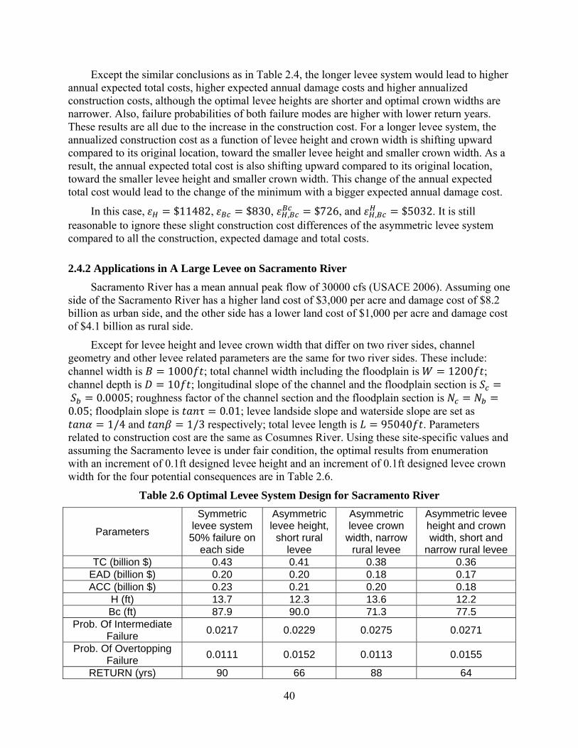
40

Except the similar conclusions as in Table 2.4, the longer levee system would lead to higher annual expected total costs, higher expected annual damage costs and higher annualized construction costs, although the optimal levee heights are shorter and optimal crown widths are narrower. Also, failure probabilities of both failure modes are higher with lower return years. These results are all due to the increase in the construction cost. For a longer levee system, the annualized construction cost as a function of levee height and crown width is shifting upward compared to its original location, toward the smaller levee height and smaller crown width. As a result, the annual expected total cost is also shifting upward compared to its original location, toward the smaller levee height and smaller crown width. This change of the annual expected total cost would lead to the change of the minimum with a bigger expected annual damage cost.

In this case, $11482, $830, , $726, and , $5032. It is still reasonable to ignore these slight construction cost differences of the asymmetric levee system compared to all the construction, expected damage and total costs.

2.4.2 Applications in A Large Levee on Sacramento River

Sacramento River has a mean annual peak flow of 30000 cfs (USACE 2006). Assuming one side of the Sacramento River has a higher land cost of $3,000 per acre and damage cost of $8.2 billion as urban side, and the other side has a lower land cost of $1,000 per acre and damage cost of $4.1 billion as rural side.

Except for levee height and levee crown width that differ on two river sides, channel geometry and other levee related parameters are the same for two river sides. These include: channel width is 1000 ; total channel width including the floodplain is 1200 ; channel depth is 10 ; longitudinal slope of the channel and the floodplain section is 0.0005; roughness factor of the channel section and the floodplain section is 0.05; floodplain slope is τ 0.01; levee landside slope and waterside slope are set as

1/4 and 1/3 respectively; total levee length is 95040 . Parameters related to construction cost are the same as Cosumnes River. Using these site-specific values and assuming the Sacramento levee is under fair condition, the optimal results from enumeration with an increment of 0.1ft designed levee height and an increment of 0.1ft designed levee crown width for the four potential consequences are in Table 2.6.

Table 2.6 Optimal Levee System Design for Sacramento River

Parameters

Symmetric levee system

50% failure on each side

Asymmetric levee height,

short rural levee

Asymmetric levee crown

width, narrow rural levee

Asymmetric levee height and crown width, short and

narrow rural levee TC (billion $) 0.43 0.41 0.38 0.36

EAD (billion $) 0.20 0.20 0.18 0.17 ACC (billion $) 0.23 0.21 0.20 0.18

H (ft) 13.7 12.3 13.6 12.2 Bc (ft) 87.9 90.0 71.3 77.5

Prob. Of Intermediate Failure

0.0217 0.0229 0.0275 0.0271

Prob. Of Overtopping Failure

0.0111 0.0152 0.0113 0.0155

RETURN (yrs) 90 66 88 64

41

Similar conclusions can be achieved that the asymmetric levee system with a short and narrow rural levee and a high and wide urban levee is the most economically optimal design with the lowest annual expected total cost, as well as a lowest expected annual damage cost and a lowest annualized construction cost. And all the asymmetric levee systems are more cost-effective than the symmetric levee system in terms of annual expected total cost. Among the three asymmetric levee systems, optimal levee height remains fairly constant compared to the changes of optimal levee crown width, which are all smaller than those of the symmetric levee system. This also leads to the bigger changes in the probability of intermediate geotechnical failure than in the probability of overtopping failure. Additionally, the intermediate geotechnical failure is about twice likely to occur than the overtopping failure for each of the four optimally design levee system, which again demonstrate the importance of including the intermediate geotechnical failure in the risk-based analysis for optimal levee design.

In this case, the construction cost difference of the asymmetric levee system with only asymmetric levee height is $824,493, with only asymmetric levee crown width is$97,732, with asymmetric levee height and asymmetric levee crown width is , $92,129 for the crown width difference and , $734,854 for the height difference. Compared to the annual expected total cost, expected annual damage cost and annualized construction cost, it is reasonable to ignore these slight construction cost differences of the asymmetric levee system, especially the difference between a narrow levee and a wide levee.

As different levee conditions would affect the intermediate geometrical failure probability, we can compare the optimal results of levee system design under different levee conditions. Assuming the levee system on Sacramento River is under good condition, the optimal results for the four potential consequences are in Table 2.7.

Table 2.7 Optimal Levee System Design for Sacramento River, Assuming Good Levees

Parameters

Symmetric levee system

50% failure on each side

Asymmetric levee height,

short rural levee

Asymmetric levee crown

width, narrow rural levee

Asymmetric levee height and crown width, short and

narrow rural levee TC (billion $) 0.29 0.28 0.26 0.24

EAD (billion $) 0.13 0.13 0.11 0.11 ACC (billion $) 0.16 0.15 0.15 0.13

H (ft) 16.6 15.1 15.7 14.7 Bc (ft) 20.0 26.4 20.0 20.0

Prob. Of Intermediate Failure

0.0152 0.0155 0.0166 0.0184

Prob. Of Overtopping Failure

0.0060 0.0082 0.0072 0.0089

RETURN (yrs) 167 122 139 112

Other than the similar conclusions as from Table 2.6, the good levee systems tend to have lower annual expected total costs, lower expected annual damage costs and lower annualized construction costs. The optimal levee heights are higher as to balance the decrease in intermediate geotechnical failures. Correspondingly, the optimal crown widths are much narrower that three of them even reach the lower limits of design crown width. Also, failure probabilities of both failure modes are lower with higher return years. These results are all due to

42

the decrease in the intermediate geotechnical failure of a good levee. For a better levee system, the expected annual damage cost is shifting downward compared to its original location, toward the smaller levee height and smaller crown width. As a result, the annual expected total cost is also shifting downward compared to its original location, toward the smaller levee height and smaller crown width. This change of the annual expected total cost would lead to the change of the minimum with a smaller annualize construction cost.

2.5 Conclusion

This study examines the optimal design of a common simple levee system with two levees on opposite riverbanks. Risk-based analysis for minimizing overall annual expected total cost is used to demonstrate the economic optimality of an asymmetric levee system mathematically and analytically. For overtopping failure, intermediate geotechnical failure or a combination of these two failures, asymmetric levee system is proved to be the most economic efficient design under the assumption that the slight difference of construction cost can be reasonably ignored. Specifically, the optimal levee system design would always transferring the entire flood risk to the low-valued riverside for any failure modes. In particular, one would always build a relatively low and narrow levee on the low-valued to undertake all the likely flood damages from overtopping failure and intermediate geotechnical failure. With the overall economic optimality of designing asymmetric levee systems to transfer flood risk, individual costs generally increase. In order to improve conditions for all parties, compensation for transferred flood risk should be negotiated and guaranteed.

2.6 References

Apel, H., Thieken, A. H., Merz, B., & Blöschl, G. (2004). Flood risk assessment and associated uncertainty. Natural Hazards and Earth System Science, 4(2), 295-308.

Croghan, L. (2013). Economic Model for Optimal Flood Risk Transfer. Master’s Thesis. Plate, E. J. (2002). Flood risk and flood management. Journal of Hydrology, 267(1), 2-11. Hashimoto, T., J. R. Stedinger, and D. P. Loucks (1982), Reliability, resiliency, and vulnerability

criteria for water resource system performance evaluation, Water Resour. Res., 18(1), 14–20.

Tung, Y.-K., and L. W. Mays (1981a), Risk models for flood levee design, Water Resour. Res., 17(4), 833–841.

Tung, Y.-K., and L. W. Mays (1981b), Optimal risk-based design of flood levee systems, Water Resour. Res., 17(4), 843–852.

USACE (2006), TL 1110-2-561, Reliability Analysis and Risk Assessment for Seepage and Slope Stability Failure Modes for Embankment Dams.

2.7 Appendixes

2.7.A Economic Optimality of the Asymmetric Levee Height

Considering overtopping failure only with symmetric levee crown width, the objectives of minimizing total cost for the four listed potential consequences in section 2.3.2 are in the following. All damages are assumed to occur once the levee fails.

(1) Symmetric levee height with simultaneous levee failures on both sides

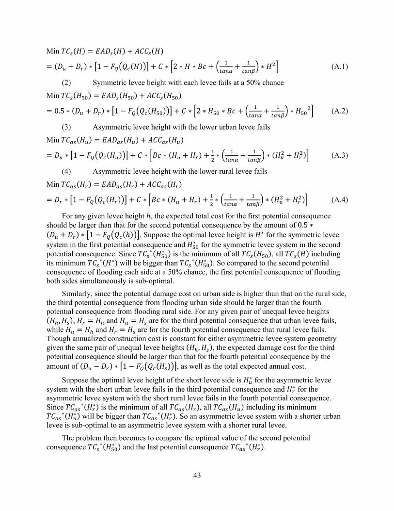
43

Min

∗ 1 ∗ 2 ∗ ∗ ∗ (A.1)

(2) Symmetric levee height with each levee fails at a 50% chance

Min

0.5 ∗ ∗ 1 ∗ 2 ∗ ∗ ∗ (A.2)

(3) Asymmetric levee height with the lower urban levee fails

Min

∗ 1 ∗ ∗ ∗ ∗ (A.3)

(4) Asymmetric levee height with the lower rural levee fails

Min

∗ 1 ∗ ∗ ∗ ∗ (A.4)

For any given levee height , the expected total cost for the first potential consequence should be larger than that for the second potential consequence by the amount of 0.5 ∗

∗ 1 . Suppose the optimal levee height is ∗ for the symmetric levee system in the first potential consequence and ∗ for the symmetric levee system in the second potential consequence. Since ∗ ∗ is the minimum of all , all including its minimum ∗ ∗ will be bigger than ∗ ∗ . So compared to the second potential consequence of flooding each side at a 50% chance, the first potential consequence of flooding both sides simultaneously is sub-optimal.

Similarly, since the potential damage cost on urban side is higher than that on the rural side, the third potential consequence from flooding urban side should be larger than the fourth potential consequence from flooding rural side. For any given pair of unequal levee heights

, , and are for the third potential consequence that urban levee fails, while and are for the fourth potential consequence that rural levee fails. Though annualized construction cost is constant for either asymmetric levee system geometry given the same pair of unequal levee heights , , the expected damage cost for the third potential consequence should be larger than that for the fourth potential consequence by the amount of ∗ 1 , as well as the total expected annual cost.

Suppose the optimal levee height of the short levee side is ∗ for the asymmetric levee system with the short urban levee fails in the third potential consequence and ∗ for the asymmetric levee system with the short rural levee fails in the fourth potential consequence. Since ∗ ∗ is the minimum of all , all including its minimum

∗ ∗ will be bigger than ∗ ∗ . So an asymmetric levee system with a shorter urban levee is sub-optimal to an asymmetric levee system with a shorter rural levee.

The problem then becomes to compare the optimal value of the second potential consequence ∗ ∗ and the last potential consequence ∗ ∗ .

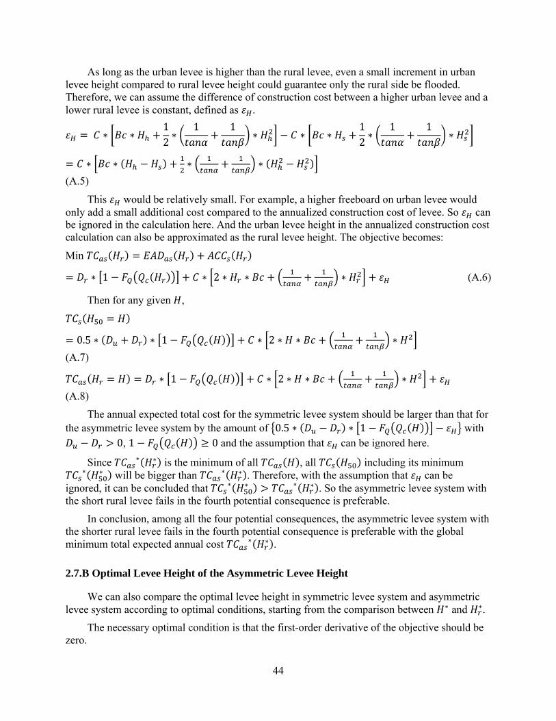
44

As long as the urban levee is higher than the rural levee, even a small increment in urban levee height compared to rural levee height could guarantee only the rural side be flooded. Therefore, we can assume the difference of construction cost between a higher urban levee and a lower rural levee is constant, defined as .

∗ ∗12∗

1 1∗ ∗ ∗

12∗

1 1∗

∗ ∗ ∗ ∗

(A.5)

This would be relatively small. For example, a higher freeboard on urban levee would only add a small additional cost compared to the annualized construction cost of levee. So can be ignored in the calculation here. And the urban levee height in the annualized construction cost calculation can also be approximated as the rural levee height. The objective becomes:

Min

∗ 1 ∗ 2 ∗ ∗ ∗ (A.6)

Then for any given ,

0.5 ∗ ∗ 1 ∗ 2 ∗ ∗ ∗

(A.7)

∗ 1 ∗ 2 ∗ ∗ ∗

(A.8)

The annual expected total cost for the symmetric levee system should be larger than that for the asymmetric levee system by the amount of 0.5 ∗ ∗ 1 with

0, 1 0 and the assumption that can be ignored here.

Since ∗ ∗ is the minimum of all , all including its minimum ∗ ∗ will be bigger than ∗ ∗ . Therefore, with the assumption that can be

ignored, it can be concluded that ∗ ∗ ∗ ∗ . So the asymmetric levee system with the short rural levee fails in the fourth potential consequence is preferable.

In conclusion, among all the four potential consequences, the asymmetric levee system with the shorter rural levee fails in the fourth potential consequence is preferable with the global minimum total expected annual cost ∗ ∗ .

2.7.B Optimal Levee Height of the Asymmetric Levee Height

We can also compare the optimal levee height in symmetric levee system and asymmetric levee system according to optimal conditions, starting from the comparison between ∗ and ∗.

The necessary optimal condition is that the first-order derivative of the objective should be zero.

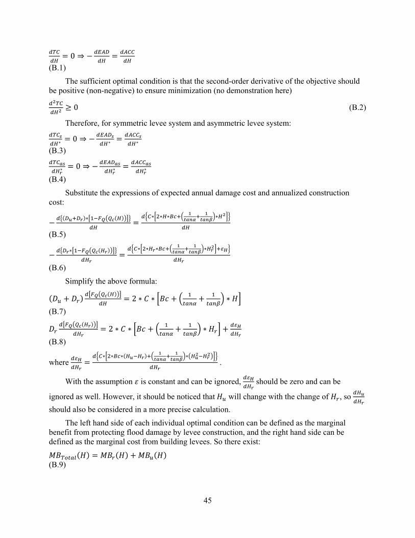
45

0 ⇒

(B.1)

The sufficient optimal condition is that the second-order derivative of the objective should be positive (non-negative) to ensure minimization (no demonstration here)

0 (B.2)

Therefore, for symmetric levee system and asymmetric levee system:

∗ 0 ⇒ ∗ ∗

(B.3)

∗ 0 ⇒ ∗ ∗

(B.4)

Substitute the expressions of expected annual damage cost and annualized construction cost:

∗ ∗ ∗ ∗ ∗

(B.5)

∗ ∗ ∗ ∗ ∗

(B.6)

Simplify the above formula:

2 ∗ ∗ ∗

(B.7)

2 ∗ ∗ ∗

(B.8)

where ∗ ∗ ∗ ∗

.

With the assumption is constant and can be ignored, should be zero and can be

ignored as well. However, it should be noticed that will change with the change of , so

should also be considered in a more precise calculation.

The left hand side of each individual optimal condition can be defined as the marginal benefit from protecting flood damage by levee construction, and the right hand side can be defined as the marginal cost from building levees. So there exist:

(B.9)

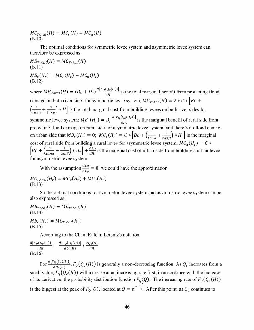
46

(B.10)

The optimal conditions for symmetric levee system and asymmetric levee system can therefore be expressed as:

(B.11)

(B.12)

where is the total marginal benefit from protecting flood

damage on both river sides for symmetric levee system; 2 ∗ ∗

∗ is the total marginal cost from building levees on both river sides for

symmetric levee system; is the marginal benefit of rural side from

protecting flood damage on rural side for asymmetric levee system, and there’s no flood damage

on urban side that 0; ∗ ∗ is the marginal

cost of rural side from building a rural levee for asymmetric levee system; ∗

∗ is the marginal cost of urban side from building a urban levee

for asymmetric levee system.

With the assumption 0, we could have the approximation:

(B.13)

So the optimal conditions for symmetric levee system and asymmetric levee system can be also expressed as:

(B.14)

(B.15)

According to the Chain Rule in Leibniz's notation

∗

(B.16)

For , is generally a non-decreasing function. As increases from a

small value, will increase at an increasing rate first, in accordance with the increase of its derivative, the probability distribution function . The increasing rate of

is the biggest at the peak of , located at . After this point, as continues to

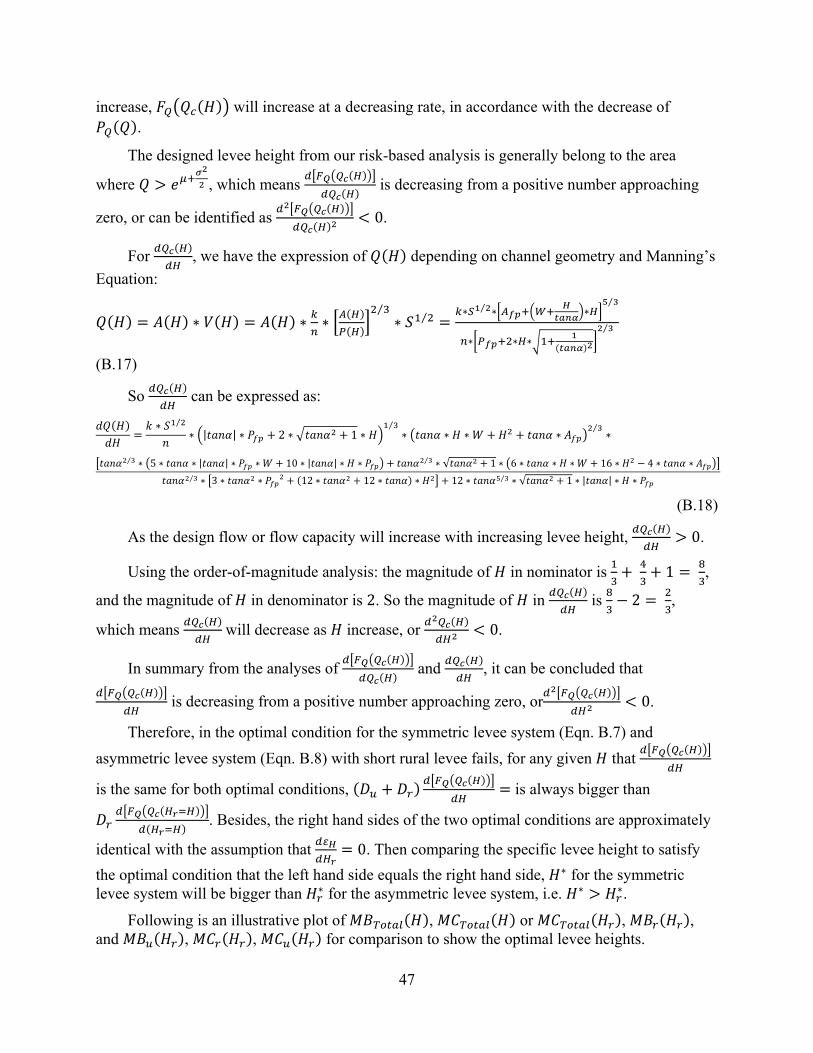
47

increase, will increase at a decreasing rate, in accordance with the decrease of .

The designed levee height from our risk-based analysis is generally belong to the area

where , which means is decreasing from a positive number approaching

zero, or can be identified as 0.

For , we have the expression of depending on channel geometry and Manning’s

Equation:

∗ ∗ ∗⁄∗ ⁄ ∗ ⁄ ∗ ∗

⁄

∗ ∗ ∗⁄

(B.17)

So can be expressed as:

∗ ⁄

∗ | | ∗ 2 ∗ 1 ∗⁄∗ ∗ ∗ ∗

⁄∗

⁄ ∗ 5 ∗ ∗ | | ∗ ∗ 10 ∗ | | ∗ ∗ ⁄ ∗ √ 1 ∗ 6 ∗ ∗ ∗ 16 ∗ 4 ∗ ∗⁄ ∗ 3 ∗ ∗ 12 ∗ 12 ∗ ∗ 12 ∗ ⁄ ∗ √ 1 ∗ | | ∗ ∗

(B.18)

As the design flow or flow capacity will increase with increasing levee height, 0.

Using the order-of-magnitude analysis: the magnitude of in nominator is 1 ,

and the magnitude of in denominator is 2. So the magnitude of in is 2 ,

which means will decrease as increase, or 0.

In summary from the analyses of and , it can be concluded that

is decreasing from a positive number approaching zero, or 0.

Therefore, in the optimal condition for the symmetric levee system (Eqn. B.7) and

asymmetric levee system (Eqn. B.8) with short rural levee fails, for any given that

is the same for both optimal conditions, is always bigger than

. Besides, the right hand sides of the two optimal conditions are approximately

identical with the assumption that 0. Then comparing the specific levee height to satisfy

the optimal condition that the left hand side equals the right hand side, ∗ for the symmetric levee system will be bigger than ∗ for the asymmetric levee system, i.e. ∗ ∗.

Following is an illustrative plot of , or , , and , , for comparison to show the optimal levee heights.

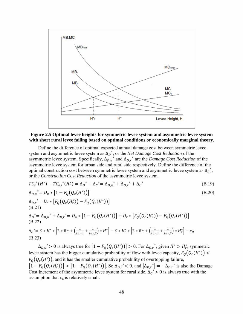
48

Figure 2.5 Optimal levee heights for symmetric levee system and asymmetric levee system with short rural levee failing based on optimal conditions or economically marginal theory.

Define the difference of optimal expected annual damage cost between symmetric levee system and asymmetric levee system as ∆ ∗, or the Net Damage Cost Reduction of the asymmetric levee system. Specifically, ∆ ,

∗ and ∆ ,∗ are the Damage Cost Reduction of the

asymmetric levee system for urban side and rural side respectively. Define the difference of the optimal construction cost between symmetric levee system and asymmetric levee system as ∆ ∗, or the Construction Cost Reduction of the asymmetric levee system.

∗ ∗ ∗ ∗ ∆ ∗ ∆ ∗ ∆ ,∗ ∆ ,

∗ ∆ ∗ (B.19)

∆ ,∗ ∗ 1 ∗ (B.20)

∆ ,∗ ∗ ∗ ∗

(B.21)

∆ ∗ ∆ ,∗ ∆ ,

∗ ∗ 1 ∗ ∗ ∗ ∗ (B.22)

∆ ∗ ∗ ∗ ∗ 2 ∗ ∗ ∗ ∗ ∗ ∗ 2 ∗ ∗ ∗

(B.23)

∆ ,∗ 0 is always true for 1 ∗ 0. For ∆ ,

∗, given ∗ ∗, symmetric levee system has the bigger cumulative probability of flow with levee capacity, ∗

∗ , and it has the smaller cumulative probability of overtopping failure, 1 ∗ 1 ∗ . So ∆ ,

∗ 0, and ∆ ,∗ ∆ ,

∗ is also the Damage Cost Increment of the asymmetric levee system for rural side. ∆ ∗ 0 is always true with the assumption that is relatively small.

49

In summary: ∆ ,∗ ∆ ∗ is the Cost Reduction of the asymmetric levee system; ∆ ,

∗ is the Cost Increment of the asymmetric levee system.

Then we have the following conclusion: if ∆ ,∗ ∆ ∗ ∆ ,

∗ , the asymmetric levee system is preferable; if

∆ ,

∗ ∆ ∗ ∆ ,∗ , the symmetric levee system is preferable.

According to the previous analysis and the assumption of ignoring , we know that the asymmetric levee system with the lower rural levee fails is preferable, so ∆ ,

∗ ∆ ∗ ∆ ,∗ ,

Cost Reduction exceeds Cost Increment of the asymmetric levee system.

Similarly, we can compare the optimal levee height between ∗ and ∗.

Similar to Eqn. B.5 and Eqn. B.6,

. ∗ ∗ ∗ ∗ ∗ ∗

(B.24)

∗ ∗ ∗ ∗ ∗

(B.25)

Simplify the above formula and similar to Eqn. B.7 and Eqn. B.8:

0.5 ∗ 2 ∗ ∗ ∗

(B.26)

2 ∗ ∗ ∗

(B.27)

where ∗ ∗ ∗ ∗

.

The optimal levee heights similar to Eqn. (B.9) and Eqn. (B.10) are:

0.5 ∗ (B.28)

(B.29)

Then the optimal conditions can be also expressed as:

(B.30)

(B.31)

where 0.5 ∗ is the total marginal benefit from

protecting flood damage on both river sides for symmetric levee system; 2 ∗

50

∗ ∗ is the total marginal cost from building levees on both river sides

for symmetric levee system; , and are the same above.

With the assumption 0, we could have the approximation:

(B.32)

So the optimal conditions can be also expressed as:

(B.33)

(B.34)

According to the same analytical discussion above, in the optimal condition for the symmetric levee system (Eqn. B.26) and asymmetric levee system (Eqn. B.27) with short rural

levee fails, for any given that is the same for both optimal conditions, 0.5 ∗

is always bigger than . Besides, the right hand sides

of the two optimal conditions are approximately identical with the assumption that 0.

Then comparing the specific levee height to satisfy the optimal condition that the left hand side equals the right hand side, ∗ for the symmetric levee system with each levee fails at a 50% chance will be bigger than ∗ for the asymmetric levee system with short rural levee fails, i.e. ∗ ∗.

Following is an illustrative plot of , or , , and , , for comparison to show the optimal levee heights.

51

Figure 2.6 Optimal levee heights for symmetric levee system with each levee fails at a 50% chance and asymmetric levee system with short rural levee fails based on optimal

conditions or economically marginal theory

Then we have similar to Eqn. B.19 to B.23: ∗ ∗ ∗ ∗ ∆ ∗ ∆ ∗ ∆ ,

∗ ∆ ,∗ ∆ ∗

(B.35)

∆ ,∗ 0.5 ∗ ∗ 1 ∗

(B.36)

∆ ,∗ 0.5 ∗ ∗ ∗ ∗

(B.37)

∆ ∗ ∆ ,∗ ∆ ,

∗ 0.5 ∗ ∗ 1 ∗ 0.5 ∗ ∗ ∗ ∗ (B.38)

∆ ∗ ∗ ∗ ∗ 2 ∗ ∗ ∗ ∗ ∗ ∗ 2 ∗ ∗ ∗

(B.39)

∆ ,∗ 0 is always true for 1 ∗ 0. For ∆ ,

∗, given ∗ ∗, symmetric levee system has the bigger cumulative probability of flow with leveed channel capacity,

∗ ∗ , and it has the smaller cumulative probability of overtopping failure, 1 ∗ 1 ∗ . So ∆ ,

∗ 0, and ∆ ,∗ ∆ ,

∗ is also the Damage Cost Increment of the asymmetric levee system for rural side. ∆ ∗ 0 is always true with the assumption that is relatively small.

In summary: ∆ ,∗ ∆ ∗ is the Cost Reduction of the asymmetric levee system; ∆ ,

∗ is the Cost Increment of the asymmetric levee system.

Then we have the following conclusion:

If ∆ ,∗ ∆ ∗ ∆ ,

∗ , the asymmetric levee system with short rural levee fails is preferable.

If ∆ ,

∗ ∆ ∗ ∆ ,∗ , the symmetric levee system with each levee fails at a 50% chance

is preferable.

According to the previous analysis and the assumption of ignoring , we know that the asymmetric levee system with the short rural levee fails is preferable, so ∆ ,

∗ ∆ ∗ ∆ ,∗ ,

Cost Reduction exceeds Cost Increment of the asymmetric levee system.

2.7.C Economic Optimality of the Asymmetric Levee Crown Width

Considering intermediate geotechnical failure only with symmetric levee height, the objectives of minimizing total cost for the four listed potential consequences in section 2.3.3 are in the following. All damages are assumed to occur once the levee fails.

(1) Symmetric levee crown width with simultaneous levee failures on both sides

Min

52

∗ ∗ , ∗ 2 ∗ ∗ ∗ (C.1)

(2) Symmetric levee crown width with each levee fails at a 50% chance

Min

0.5 ∗ ∗ ∗ , ∗ 2 ∗ ∗ ∗

(C.2)

(3) Asymmetric levee crown width with the narrow urban levee fails

Min

∗ ∗ , ∗ ∗ ∗ (C.3)

(4) Asymmetric levee crown width with the lower rural levee fails

Min

∗ ∗ , ∗ ∗ ∗ (C.4)

For any given , the expected total cost of the first potential consequence should be larger than that of the second potential consequence by the amount of 0.5 ∗ ∗

∗ , . Suppose the optimal levee crown width is ∗ for the symmetric levee system in the first potential consequence and ∗ for the symmetric levee system in the second potential consequence. Since ∗ ∗ is the minimum of all , all including its minimum ∗ ∗ will be bigger than ∗ ∗ . So compared to the second potential consequence of flooding each side at a 50% chance, the first potential consequence of flooding both sides simultaneously is sub-optimal.

Similarly, based on the assumption that the potential damage cost on urban side is higher than that on the rural side, the third potential consequence from flooding urban side should be larger than the fourth potential consequence from flooding rural side. For any given pair of unequal levee crown widths , , and are for the third potential consequence that urban levee fails, while and are for the fourth potential consequence that rural levee fails. Though annualized construction cost is constant for either asymmetric levee system geometry given the same pair of unequal levee crown widths

, , the expected damage cost for the third potential consequence should be larger than

that for the fourth potential consequence by the amount of ∗ ∗, , as well as the total expected annual cost.

Suppose the optimal levee crown width of the narrow levee side is ∗ for the asymmetric levee system with the narrow urban levee fails in the third potential consequence and ∗ for the asymmetric levee system with the narrow rural levee fails in the fourth potential consequence. Since ∗ ∗ is the minimum of all , all including its minimum

∗ ∗ will be bigger than ∗ ∗ . So an asymmetric levee system with a narrow urban levee is sub-optimal to an asymmetric levee system with a narrow rural levee.

The problem then becomes to compare the optimal value of the second potential consequence ∗ ∗ and the last potential consequence ∗ ∗ .

53

According to our simplifying assumption that the intermediate geotechnical failure probability of a comparatively narrow levee is always greater than that of a wide levee at any water level, as long as the urban levee is wide than that he rural levee, even a small increment in urban levee crown width compared to rural levee crown width could guarantee only the rural side be flooded. Therefore, we can assume the difference of construction cost between a wide urban levee and a narrow rural levee is constant, defined as .

∗ ∗12∗

1 1∗

∗ ∗12∗

1 1∗

= ∗ ∗ (C.5)

This can be relatively small, in which case can be ignored and the urban levee crown width in the annualized construction cost calculation can also be approximated as the rural levee crown width. The objective becomes:

Min

∗ ∗ , ∗ 2 ∗ ∗ ∗ (C.6)

Then for any given ,

0.5 ∗ ∗ ∗ , ∗ 2 ∗ ∗

∗ (C.7)

∗ ∗ , ∗ 2 ∗ ∗ ∗

(C.8)

The annual expected total cost of the symmetric levee system should be larger than that of

the asymmetric levee system by 0.5 ∗ ∗ ∗ , with

0, ∗ , 0 and the assumption that can be ignored here.

Since ∗ ∗ is the minimum of all , all including its minimum ∗ ∗ will be bigger than ∗ ∗ . Therefore, with the assumption that can be

ignored, it can be concluded that ∗ ∗ ∗ ∗ . So the asymmetric levee system with the narrow rural levee fails in the fourth potential consequence is preferable.

In conclusion, among all the four potential consequences, the asymmetric levee system with the narrow rural levee fails in the fourth potential consequence is preferable with the global minimum total expected annual cost ∗ ∗ .

2.7.D Economic Optimality of the Asymmetric Levee System Geometry

Considering both the overtopping failure and intermediate geotechnical failure, the objectives of minimizing total cost for the four listed potential consequences in section 2.3.4 are in the following. All damages are assumed to occur once the levee fails.

54

(1) Symmetric levee system with each levee fails at a 50% chance, ,

Min , , ,

0.5 ∗ ∗ 1 0.5 ∗ ∗ ∗ ,

∗ 2 ∗ ∗ ∗ (D.1)

(2) Asymmetric levee system with asymmetric levee height and symmetric levee crown width, overtopping failure occurs on short rural levee side, intermediate geotechnical failure occurs on each side at a 50% chance, , ,

Min , , ,

∗ 1 0.5 ∗ ∗ ∗ , ∗ ∗

∗ ∗ (D.2)

(3) Asymmetric levee system with symmetric levee height and asymmetric levee crown width, overtopping failure occurs on each side at a 50% chance, intermediate geotechnical failure occurs on narrow rural levee side, , ,

Min , , ,

0.5 ∗ ∗ 1 ∗ ∗ , ∗

∗ ∗ (D.3)

(4) Asymmetric levee system with asymmetric levee height and asymmetric levee crown width, overtopping failure and intermediate geotechnical failures occur on short and narrow rural levee side, , , ,

Min , , ,

∗ 1 ∗ ∗ , ∗ ∗ ∗

∗ ∗ (D.4)

According to previous discussion, ∗ ∗ , ∗ in the first potential consequence is suboptimal to ∗ ∗, ∗ in the second potential consequence by the amount of 0.5 ∗ ∗ 1 assuming that can be ignored. And

∗ ∗ , ∗ in the first potential consequence is suboptimal to ∗ ∗ , ∗ in the third

potential consequence by the amount of 0.5 ∗ ∗ ∗ ,

assuming that can be ignored. and are from Equation (A.5) and (B.5) respectively.

So the economically optimal design of the levee system geometry should be chosen from ∗ ∗, ∗ in the second potential consequence, ∗ ∗ , ∗ in the third potential

consequence and ∗ ∗, ∗ in the last potential consequence.

55

First we compare ∗ ∗, ∗ in the second potential consequence and ∗ ∗, ∗ in the last potential consequence. The difference of construction cost between these two potential consequences is defined as , .

,

∗ ∗ ∗12∗

1 1∗

∗ ∗12∗

1 1∗

∗ ∗ ∗ ∗ (D.5)

Given in our analysis,

, ∗ ∗ (D.6)

This , would be relatively small, in which case , can be ignored. And the urban levee in the annualized construction cost calculation can also be approximated as the rural levee.

For any given ,

,

∗ 1 0.5 ∗ ∗ ∗ , ∗ ∗

∗ ∗ (D.7)

,

∗ 1 ∗ ∗ , ∗ ∗ ∗

∗ , (D.8)

The annual expected total cost in the second potential consequence should be larger than

that in the last potential consequence by the amount of 0.5 ∗ ∗ ∗

, , with 0, ∗ , 0 and the

assumption that , can be ignored here.

Since ∗ ∗, ∗ is the minimum of all , , all , including its minimum ∗ ∗, ∗ will be bigger than ∗ ∗, ∗ . Therefore, with the assumption that , can be ignored, it can be concluded that ∗ ∗, ∗ ∗ ∗, ∗ . So the asymmetric levee system with the short and narrow rural levee fails in the last potential consequence is preferable.

Then we compare ∗ ∗ , ∗ in the third potential consequence and ∗ ∗, ∗ in the last potential consequence. The difference of construction cost between these two potential consequences is defined as , .

,

∗ ∗ ∗12∗

1 1∗

56

∗ ∗ ∗

(D.9)

Given in our analysis,

, ∗ ∗ ∗ ∗

(D.10)

This , would be relatively small, in which case , can be ignored. And the urban levee in the annualized construction cost calculation can also be approximated as the rural levee.

For any given ,

,

0.5 ∗ ∗ 1 ∗ ∗ , ∗

∗ ∗ (D.11)

,

∗ 1 ∗ ∗ , ∗ ∗

∗ , (D.12)

The annual expected total cost in the third potential consequence should be larger than that in the last potential consequence by the amount of 0.5 ∗ ∗ 1 , with 0, 1 0 and the assumption that , can be ignored here.

Since ∗ ∗, ∗ is the minimum of all , , all , including its minimum ∗ ∗ , ∗ will be bigger than ∗ ∗, ∗ . Therefore, with the assumption that , can be ignored, it can be concluded that ∗ ∗ , ∗ ∗ ∗, ∗ . So the asymmetric levee system with the short and narrow rural levee fails in the last potential consequence is preferable.

In conclusion, among all the four potential consequences, the asymmetric levee system with asymmetric levee height and asymmetric levee crown width is of the overall economic optimality. Specifically, the short and narrow rural levee fails in the fourth potential consequence is preferable with the global minimum total expected annual cost ∗ ∗, ∗ .

57

Chapter 3: Game Theory and Risk-Based Levee System Design

3.1 Summary

Optimal risk-based levee design is usually developed for economic efficiency. However, in many river systems, the design and operation of different levees are controlled by different agencies. For example, along many rivers, levees on opposite riverbanks are a simple levee system with each levee owned separately. Collaborative design of the two levees can be economically optimal for the whole system. But rational and self-interested land owners on each river bank often tend to independently optimize their levees, resulting in a Pareto-inefficient levee system design from a society-wide perspective. Game theory is applied in this study to analyze decision-making in a simple levee system where land owners on each river bank develop levee designs using risk-based economic optimization. For each land owner, the annual expected total cost includes expected annual damage cost and annualized construction cost. The non-cooperative Nash equilibrium is identified and compared to the optimal distribution of flood risk and damage cost, which minimizes total flood cost system-wide. The system-wide optimal solution often is not feasible politically or legally without compensating for the transferred flood risk to guarantee and improve outcomes for all parties. Such compensation can be determined and implemented in practice using cooperative game theory with landowners’ agreements on collaboration to develop an economically optimal design. By examining the successive repeated non-cooperative game in reversible and irreversible decision modes, the cost of decision making myopia can be calculated to show the significance of considering the externalities and evolution path of dynamic water resource problems for optimal decision making.

3.2 Introduction

Levees protect flood prone areas by increasing channel capacity to retain flood flow within the leveed channel rather than overflowing a protected area. However, levees possibly fail by the overtopping and intermediate geotechnical failures, though at a low probability. As risk is the failure probability multiplied by the consequences of failure, summed over all possible events, levees can decrease but cannot eliminate the likelihood of flooding and flood risk (Hashimoto et al. 1982).

Risk-based analysis has long been applied to optimal levee design, for example the basic risk models for flood levee design which systematically analyzed the various hydrologic and hydraulic uncertainties (Van Dantzig 1956; Tung and Mays 1981a), and a recent study of single levee design considering both overtopping and intermediate geotechnical failures (Chapter 1). Building a taller and wider levee decreases its failure probability and reduces its damage cost, but increases its construction cost. The optimal system design should minimize annual expected total cost, including both expected annual damage and annualized construction costs. For a levee system of two levees on opposite riverbanks, the overall cost on two sides from damage and construction should be optimized with risk-based analysis.

Different levee system designs change how flood risk is distributed. A symmetric levee system has two identical levees that possibly fail at the same chance, while the relatively lower levee in an asymmetric levee system is more likely to fail. Croghan (2013) discussed the economic flood risk transformation and transference among floodplain users, finding that total flood risk could be reduced from transferring risk from the high-cost urban side to the low-

58

valued rural side of a river. Chapter 2 provides the theoretical and numerical foundation that such an asymmetric levee system allowing flood risk transfer across the river can also reduce the total cost containing construction for asymmetric river channel system. It proves the overall economic optimality of such asymmetric levee system mathematically and analytically. However, as individual costs usually increase with transferred flood risk, compensation for the transferred flood risk can be needed to guarantee and improve conditions for all parties.

Many quantitative and qualitative methods have been proposed for water resources conflict resolution studies, for example Shared Vision Modeling (Lund and Palmer 1997) and descriptive methods for prevention and resolution of water resources conflict (Wolff 2002). A mathematical study on the interaction among independently self-interested agents, known as game theory, can be applied to analyze the design strategy of each floodplain as two individual owners involved in a levee system. Nash (1951; 1953) developed explicit theories for two types of games: cooperative games where all stakeholders collaborate, and non-cooperative games where each stakeholder acts independently with incentives to disregard the common good. The main application of game theory has been in economics, but it has been applied in many fields, such as computer science, political science, biology and psychology (Neumann 1947; Ostrom 1998; Colman 2013). Many researches have applied game-theoretic framework to water conflict resolution studies (Carraro et al. 2005; Parrachino et al. 2006; Zara et al. 2006). Madani (Madani 2010) has reviews the application of game theory to general water resources conflict management problems, particularly non-cooperative game theory. It emphasized the differences between outcomes predicted by game theory and results proposed by optimization methods assuming all parties agree to collaborate. For this simple levee system design problem, game theory can provide insights for the conditions needed to achieve the overall economically optimal levee system design, as long as the decision makers of the two river banks are rational. More importantly, compensation for the transferred flood risk can be determined by examining the risk-based levee system design solutions with different types of games and comparing their outcomes (Brandenburger 2007).

This chapter proceeds as follows. Section 3.3 describes the game theory framework and risk-based optimization for a simple levee system, including model description, risk-based analysis for overtopping failure, a simple game theory framework, and two illustrative cases of identical and different floodplain conditions on opposite riverbanks. Section 3.4 briefly employs cooperative game theory, which generates an overall economically optimal design (minimizing the annual expected total system cost). This is followed by discussions of applying different non-cooperative game conditions that require no collaboration of parties involved in the levee system design problem. Section 3.5 applies the single-shot non-cooperative Nash equilibrium game theory to this simple levee system. Sections 3.6 and 3.7 then analyze the levee system design problem as a successive repeated non-cooperative game with reversible and irreversible decisions. Section 3.8 concludes with key findings.

3.3 Risk-based Optimal Levee Design and Game Theory Framework

Risk is the sum of each possible failure event probability multiplied by its consequences, and reliability is one minus the probability of failure (Hashimoto. et al. 1982). Risk-based analysis for levee design typically minimizes the annual expected total cost, including expected annual damage and annualized construction costs. This section applies game theory to a simple

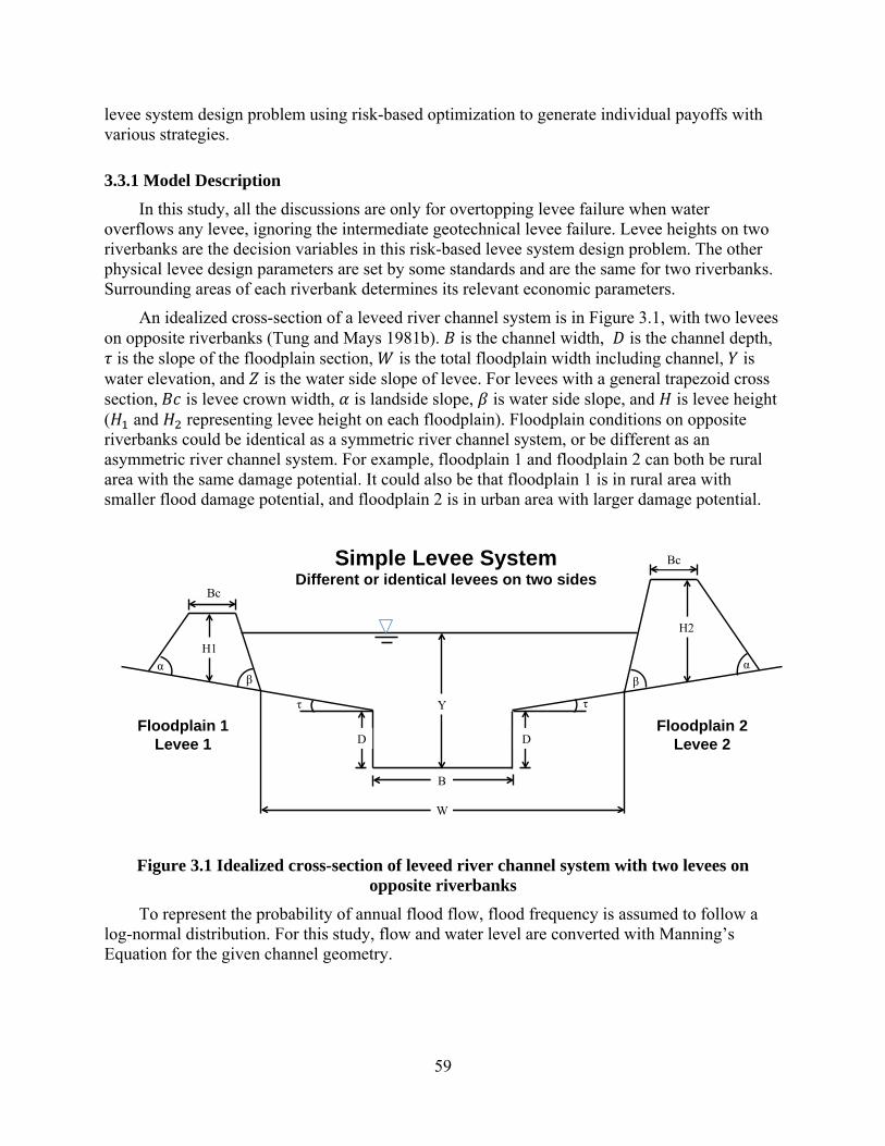
59

levee system design problem using risk-based optimization to generate individual payoffs with various strategies.

3.3.1 Model Description

In this study, all the discussions are only for overtopping levee failure when water overflows any levee, ignoring the intermediate geotechnical levee failure. Levee heights on two riverbanks are the decision variables in this risk-based levee system design problem. The other physical levee design parameters are set by some standards and are the same for two riverbanks. Surrounding areas of each riverbank determines its relevant economic parameters.

An idealized cross-section of a leveed river channel system is in Figure 3.1, with two levees on opposite riverbanks (Tung and Mays 1981b). is the channel width, is the channel depth, is the slope of the floodplain section, is the total floodplain width including channel, is

water elevation, and is the water side slope of levee. For levees with a general trapezoid cross section, is levee crown width, is landside slope, is water side slope, and is levee height ( and representing levee height on each floodplain). Floodplain conditions on opposite riverbanks could be identical as a symmetric river channel system, or be different as an asymmetric river channel system. For example, floodplain 1 and floodplain 2 can both be rural area with the same damage potential. It could also be that floodplain 1 is in rural area with smaller flood damage potential, and floodplain 2 is in urban area with larger damage potential.

Figure 3.1 Idealized cross-section of leveed river channel system with two levees on opposite riverbanks

To represent the probability of annual flood flow, flood frequency is assumed to follow a log-normal distribution. For this study, flow and water level are converted with Manning’s Equation for the given channel geometry.

Floodplain 2 Levee 2

Floodplain 1 Levee 1

W

B

Bc

H1

Y

D

τ

α β

D

τ

Bc

H2

β α

Simple Levee System Different or identical levees on two sides

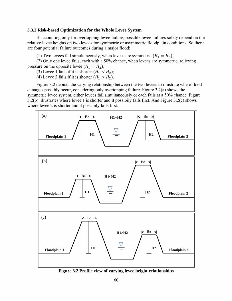
60

3.3.2 Risk-based Optimization for the Whole Levee System

If accounting only for overtopping levee failure, possible levee failures solely depend on the relative levee heights on two levees for symmetric or asymmetric floodplain conditions. So there are four potential failure outcomes during a major flood:

(1) Two levees fail simultaneously, when levees are symmetric ; (2) Only one levee fails, each with a 50% chance, when levees are symmetric, relieving

pressure on the opposite levee ; (3) Levee 1 fails if it is shorter ; (4) Levee 2 fails if it is shorter .

Figure 3.2 depicts the varying relationship between the two levees to illustrate where flood damages possibly occur, considering only overtopping failure. Figure 3.2(a) shows the symmetric levee system, either levees fail simultaneously or each fails at a 50% chance. Figure 3.2(b) illustrates where levee 1 is shorter and it possibily fails first. And Figure 3.2(c) shows where levee 2 is shorter and it possibily fails first.

Figure 3.2 Profile view of varying levee height relationships

Floodplain 1 Floodplain 2 H1 H2

Bc Bc H1=H2

Floodplain 1 Floodplain 2 H1 H2

Bc

Bc

H1<H2

Floodplain 1 Floodplain 2 H1 H2

Bc

Bc H1>H2

(a)

(b)

(c)

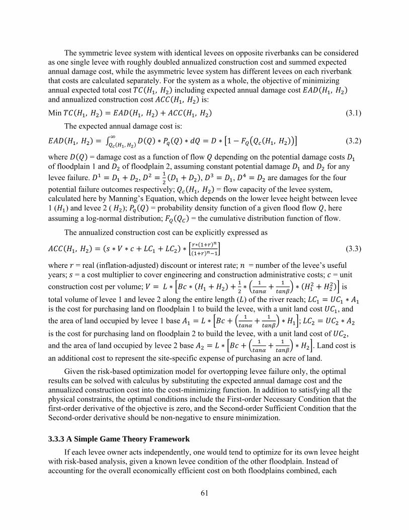
61

The symmetric levee system with identical levees on opposite riverbanks can be considered as one single levee with roughly doubled annualized construction cost and summed expected annual damage cost, while the asymmetric levee system has different levees on each riverbank that costs are calculated separately. For the system as a whole, the objective of minimizing annual expected total cost , including expected annual damage cost , and annualized construction cost , is:

Min , , , (3.1)

The expected annual damage cost is:

, ∗ ∗, ∗ 1 , (3.2)

where = damage cost as a function of flow depending on the potential damage costs of floodplain 1 and of floodplain 2, assuming constant potential damage and for any

levee failure. , , , are damages for the four

potential failure outcomes respectively; , = flow capacity of the levee system, calculated here by Manning’s Equation, which depends on the lower levee height between levee 1 ( ) and levee 2 ( ); = probability density function of a given flood flow , here assuming a log-normal distribution; = the cumulative distribution function of flow.

The annualized construction cost can be explicitly expressed as

, ∗ ∗ ∗ ∗ (3.3)

where = real (inflation-adjusted) discount or interest rate; = number of the levee’s useful years; = a cost multiplier to cover engineering and construction administrative costs; = unit

construction cost per volume; ∗ ∗ ∗ ∗ is

total volume of levee 1 and levee 2 along the entire length ( ) of the river reach; ∗ is the cost for purchasing land on floodplain 1 to build the levee, with a unit land cost , and

the area of land occupied by levee 1 base ∗ ∗ ; ∗

is the cost for purchasing land on floodplain 2 to build the levee, with a unit land cost of ,

and the area of land occupied by levee 2 base ∗ ∗ . Land cost is

an additional cost to represent the site-specific expense of purchasing an acre of land.

Given the risk-based optimization model for overtopping levee failure only, the optimal results can be solved with calculus by substituting the expected annual damage cost and the annualized construction cost into the cost-minimizing function. In addition to satisfying all the physical constraints, the optimal conditions include the First-order Necessary Condition that the first-order derivative of the objective is zero, and the Second-order Sufficient Condition that the Second-order derivative should be non-negative to ensure minimization.

3.3.3 A Simple Game Theory Framework

If each levee owner acts independently, one would tend to optimize for its own levee height with risk-based analysis, given a known levee condition of the other floodplain. Instead of accounting for the overall economically efficient cost on both floodplains combined, each

62

floodplain would try to minimize its own cost to the greatest extent, disregarding impacts on the other floodplain.

Game theory can help predict how two floodplains design their levees, following their own local interests, especially in conflict. Each floodplain is considered as one player. Each player has a set of strategies (levee design choices). Considering overtopping levee failure only, strategies would be various levee heights. Payoffs to each player for possible outcomes of the game are the individual annual expected total costs, which include expected annual damage cost and annualized construction cost. Comparing the possible payoffs can identify the dominant decisions of each player (levee heights in this case).

The payoff function for floodplain 1 is

, , (3.4)

,

0,

0.5 0.5 1 ,

1 , (3.5)

where = flow capacity of the levee system calculated by Manning’s Equation depending on the lower levee 1 height ( );

The annualized construction cost can be explicitly expressed as

∗ ∗ ∗ ∗ (3.6)

where ∗ ∗ ∗ ∗ is total volume of levee 1 along the entire

length ( ) of the river reach, is the same as discussed before.

Similarly, the payoff function for floodplain 2 is

, , (3.7)

,

0,

0.5 0.5 1 ,

1 , (3.8)

where = flow capacity of the levee system calculated by Manning’s Equation depending on the lower levee 2 height ( ).

The annualized construction cost can be explicitly expressed as

∗ ∗ ∗ ∗ (3.9)

where ∗ ∗ ∗ ∗ is total volume of levee 2 along the entire

length ( ) of the river reach, is the same as discussed before.

The payoff (annual expected total cost) of each player (floodplain 1 or floodplain 2) is a discontinuous function of the individual design levee height, because its component expected annual damage cost is discontinuous and also depends on the other player’s levee decision.

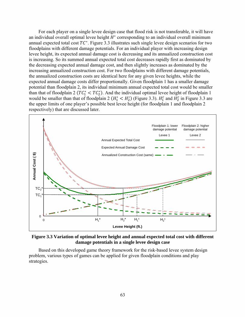
63

For each player on a single levee design case that flood risk is not transferable, it will have an individual overall optimal levee height ∗ corresponding to an individual overall minimum annual expected total cost ∗. Figure 3.3 illustrates such single levee design scenarios for two floodplains with different damage potentials. For an individual player with increasing design levee height, its expected annual damage cost is decreasing and its annualized construction cost is increasing. So its summed annual expected total cost decreases rapidly first as dominated by the decreasing expected annual damage cost, and then slightly increases as dominated by the increasing annualized construction cost. For two floodplains with different damage potentials, the annualized construction costs are identical here for any given levee heights, while the expected annual damage costs differ proportionally. Given floodplain 1 has a smaller damage potential than floodplain 2, its individual minimum annual expected total cost would be smaller than that of floodplain 2 ∗ ∗ . And the individual optimal levee height of floodplain 1 would be smaller than that of floodplain 2 ∗ ∗ (Figure 3.3). and in Figure 3.3 are the upper limits of one player’s possible best levee height (for floodplain 1 and floodplain 2 respectively) that are discussed later.

Figure 3.3 Variation of optimal levee height and annual expected total cost with different damage potentials in a single levee design case

Based on this developed game theory framework for the risk-based levee system design problem, various types of games can be applied for given floodplain conditions and play strategies.

0 0

An

nu

al C

os

t (

$)

Levee Height (ft.)

Levee 2

Annual Expected Total Cost

Levee 1

Expected Annual Damage Cost

Annualized Construction Cost (same)

H1* H2*

TC1*

TC2*

Floodplain 1: lower damage potential

Floodplain 2: higher damage potential

H1c H2

c

64

3.3.4 Illustrating Cases

To apply game theory to different levee system design institutions, we use the Cosumnes River in California as an illustrating example. Symmetric and asymmetric floodplain conditions on opposite riverbanks are analyzed as symmetric game and asymmetric game respectively (Nash 1951). For the symmetric river channel system with identical floodplain conditions on opposite riverbanks, we assume both floodplains are surrounded by rural area. For the asymmetric river channel system with different floodplain conditions, we assume floodplain 1 is in rural area and floodplain 2 is in urban area.

The Cosumnes River has a median annual peak flow of 930 and a mean annual peak flow of 1300 (USACE 2006). Channel geometry and levee related parameters include: channel width is 200 ; total channel width including the floodplain is 300 ; channel depth is 3 ; longitudinal slope of the channel and the floodplain section is 0.0005; Manning’s roughness for the channel section and floodplain is 0.05; floodplain slope is τ 0.01; levee landside slope and waterside slope are set as 1/4 and 1/2 respectively; levee crown width is 36 according to standards; total levee length is 2640 . Construction cost parameters are cost per unit levee material is

$10/ ; real (inflation-adjusted) discount or interest rate is 0.05; useful life of the levee is 100 ; the cost multiplier for engineering and construction administrative costs is

1.3.

Under the identical floodplain conditions, each rural floodplain has a land cost of $3000 per acre (0.066 $⁄ ) and roughly $8 damage cost if the surrounded area is flooded. For either floodplain optimized in a single levee design case, the individual optimal levee height is ∗ ∗ 4.3 corresponding to an individual overall minimum annual expected total cost of ∗ ∗ $0.54 , which include an expected annual damage cost of ∗

∗ $0.18 and an annualized construction cost of ∗ ∗ $0.36 . And the levee failure probability at optimal levee design is ∗ ∗ 0.0197.

Under the different floodplain conditions, rural floodplain 1 has a land cost of $3000 per acre (0.066 $⁄ ) and roughly $8 damage cost if its rural area is flooded, and urban floodplain 2 has a land cost of $9000 per acre (0.198 $⁄ ) and $20 damage cost if the surrounded urban area is flooded (USACE 2006). For rural floodplain 1 optimized in a single levee design case, the individual overall optimal levee design and costs are as above. For urban floodplain 2 optimized as a single levee design case, ∗ 5.4 , ∗ $0.74 ,

∗ $0.25 and ∗ $0.49 , and ∗ 0.01.

3.4 Cooperative Design

In a cooperative game, players make decisions collaboratively to optimize the entire system (Nash 1953). They would act together like an ideal social planner that can reach a Pareto-efficient levee system design. This is the case described in Chapter 2.

Such collaborative levee system designs are commonly seen where opposite river banks along a river belong to one land owner. A system-wide decision maker may design two identical levees for identical floodplain conditions, while would design a slightly shorter levee on low-valued floodplain for different floodplain conditions to essentially protect the other high-valued floodplain. For example with commonly different floodplain conditions, the social planner is

65

likely to sacrifice one riverbank for possible floods by designing a shorter levee on that floodplain (weirs as an extreme example). During a major flood event, this can be done by demolishing the levee on the low-valued floodplain or raising the levee on the other floodplain.

If the two floodplains on opposite riverbanks are identical, the best design for the whole system is a symmetric levee system (two identical levees) with each levee fails at a 50% chance. Under this condition, the optimal annual expected total cost ∗ ∗ with identical optimal levee heights on two riverbanks ∗ is better than any of the asymmetric levee system designs.

However, if the two floodplains on opposite riverbanks are different or it is likely that both levees would fail, an asymmetric levee system is economically optimal (Chapter 2). If the cost difference of constructing a lower rural levee 1 and a slightly higher urban levee 2, ∗

∗ ∗ ∗ , can be ignored, ∗ ∗ is economically

inferior to ∗ ∗ (Chapter 2). Therefore, the most economically optimal design of the asymmetric river channel system is a slightly shorter rural levee 1 and a slightly higher urban levee 2. The low-valued lower rural levee 1 would take all the residual flood risk by failing before the urban levee 2. Assuming only overtopping failure, the higher urban levee 2 height only has to be one additional height increment higher than the lower rural levee 1 height . So the best levee system design is the rural levee 1 at its individual optimal height as if designed as in a single levee design case, ∗ 4.3 , and the urban levee 2 slightly higher to resist all flood risk, ∗ ∗ ∆ (∆ is the design levee height increment). Compensation for the transferred flood risk should be greater than ∗ ∗ ∗ ∗ 2∆ , to guarantee that rural floodplain 1 keeps its levee height at ∗ and will not increase its levee higher than ∗. The benefit that urban floodplain 2 gains from transferring the entire flood risk to rural floodplain 1 is

∗ ∗ 2∆ , where is the equilibrium annual expected total cost of urban floodplain 2 under the competitive non-cooperative levee system design. So this benefit would be the upper limit of compensation that the urban floodplain 2 is willing to offer. varies with different institutional arrangements, as discussed below.

3.5 Single-shot Non-cooperative Game: Nash Equilibrium

Non-cooperative game theory deals with non-cooperative games in which players compete and make decisions independently (Nash 1951). In such non-cooperative games, Nash equilibrium is an outcome where no single player has an incentive to deviate unilaterally from the chosen strategy with consideration of the other players’ choices. A game may have multiple Nash equilibria or none at all. The Nash Equilibrium discussed in this study refers to only pure strategy. Future studies can analyze mixed strategies Nah Equilibrium that exist in any finite game (Nash 1950). Nash equilibrium is self-enforcing, so it is rational, but may not be economically optimal (Neumann and Morgenstern 1947). Non-cooperative game theory can help predict how levee designs where independently floodplain follows its own economic interests. In a typical non-cooperative game, decision makers (players or floodplain owners) would try to outsmart one another by anticipating each other’s decision with their own goals. Each floodplain optimizes its own objective knowing that the other floodplain’s decision affects its objective value, and knowing that its decision affects the other’s payoff and decision as well.

Levee system design is highly unusual approximated by such a single-shot non-cooperative game, as the entire design process is unlikely to be done in a negligible time period. Negotiations back and forth should be allowed. The complete levee design always includes lots discussions

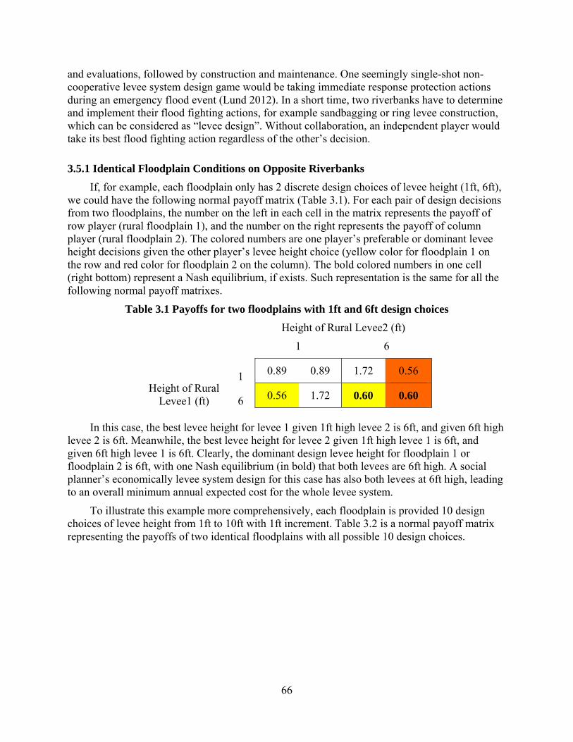
66

and evaluations, followed by construction and maintenance. One seemingly single-shot non-cooperative levee system design game would be taking immediate response protection actions during an emergency flood event (Lund 2012). In a short time, two riverbanks have to determine and implement their flood fighting actions, for example sandbagging or ring levee construction, which can be considered as “levee design”. Without collaboration, an independent player would take its best flood fighting action regardless of the other’s decision.

3.5.1 Identical Floodplain Conditions on Opposite Riverbanks

If, for example, each floodplain only has 2 discrete design choices of levee height (1ft, 6ft), we could have the following normal payoff matrix (Table 3.1). For each pair of design decisions from two floodplains, the number on the left in each cell in the matrix represents the payoff of row player (rural floodplain 1), and the number on the right represents the payoff of column player (rural floodplain 2). The colored numbers are one player’s preferable or dominant levee height decisions given the other player’s levee height choice (yellow color for floodplain 1 on the row and red color for floodplain 2 on the column). The bold colored numbers in one cell (right bottom) represent a Nash equilibrium, if exists. Such representation is the same for all the following normal payoff matrixes.

Table 3.1 Payoffs for two floodplains with 1ft and 6ft design choices

Height of Rural Levee2 (ft)

1 6

Height of Rural Levee1 (ft)

1 0.89 0.89 1.72 0.56

6 0.56 1.72 0.60 0.60

In this case, the best levee height for levee 1 given 1ft high levee 2 is 6ft, and given 6ft high

levee 2 is 6ft. Meanwhile, the best levee height for levee 2 given 1ft high levee 1 is 6ft, and given 6ft high levee 1 is 6ft. Clearly, the dominant design levee height for floodplain 1 or floodplain 2 is 6ft, with one Nash equilibrium (in bold) that both levees are 6ft high. A social planner’s economically levee system design for this case has also both levees at 6ft high, leading to an overall minimum annual expected cost for the whole levee system.

To illustrate this example more comprehensively, each floodplain is provided 10 design choices of levee height from 1ft to 10ft with 1ft increment. Table 3.2 is a normal payoff matrix representing the payoffs of two identical floodplains with all possible 10 design choices.

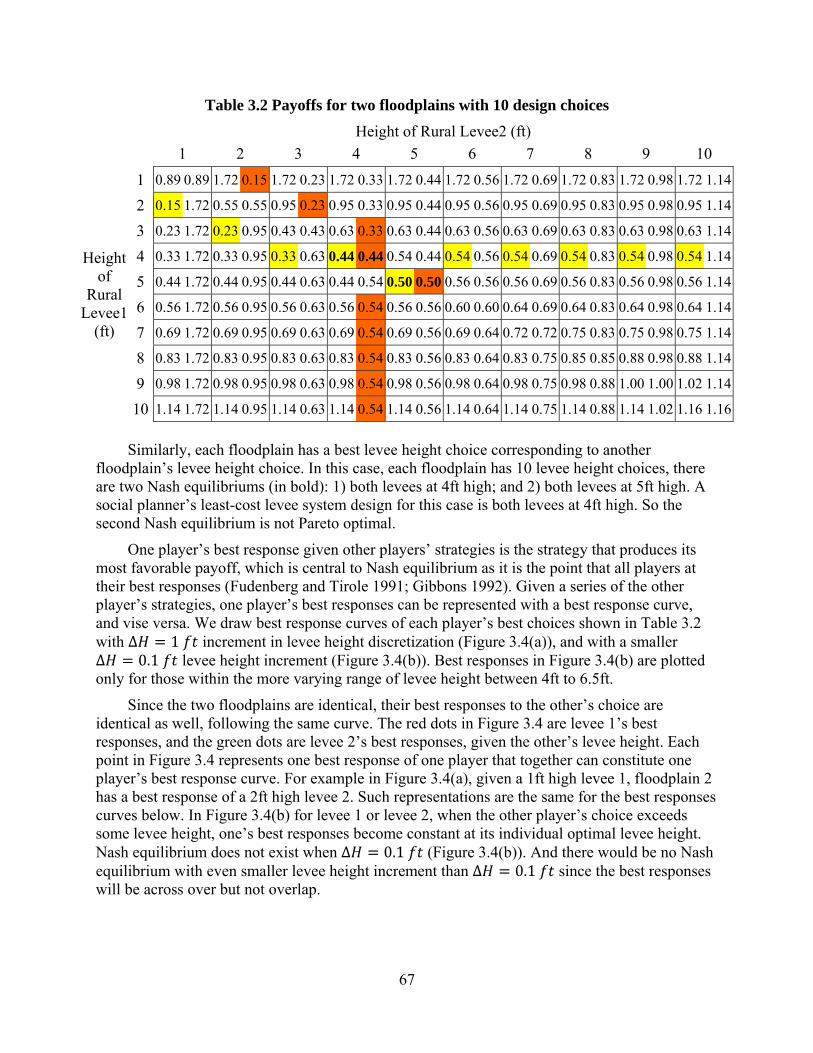
67

Table 3.2 Payoffs for two floodplains with 10 design choices

Height of Rural Levee2 (ft)

1 2 3 4 5 6 7 8 9 10

Height of

Rural Levee1

(ft)

1 0.89 0.89 1.72 0.15 1.72 0.23 1.72 0.33 1.72 0.44 1.72 0.56 1.72 0.69 1.72 0.83 1.72 0.98 1.72 1.14

2 0.15 1.72 0.55 0.55 0.95 0.23 0.95 0.33 0.95 0.44 0.95 0.56 0.95 0.69 0.95 0.83 0.95 0.98 0.95 1.14

3 0.23 1.72 0.23 0.95 0.43 0.43 0.63 0.33 0.63 0.44 0.63 0.56 0.63 0.69 0.63 0.83 0.63 0.98 0.63 1.14

4 0.33 1.72 0.33 0.95 0.33 0.63 0.44 0.44 0.54 0.44 0.54 0.56 0.54 0.69 0.54 0.83 0.54 0.98 0.54 1.14

5 0.44 1.72 0.44 0.95 0.44 0.63 0.44 0.54 0.50 0.50 0.56 0.56 0.56 0.69 0.56 0.83 0.56 0.98 0.56 1.14

6 0.56 1.72 0.56 0.95 0.56 0.63 0.56 0.54 0.56 0.56 0.60 0.60 0.64 0.69 0.64 0.83 0.64 0.98 0.64 1.14

7 0.69 1.72 0.69 0.95 0.69 0.63 0.69 0.54 0.69 0.56 0.69 0.64 0.72 0.72 0.75 0.83 0.75 0.98 0.75 1.14

8 0.83 1.72 0.83 0.95 0.83 0.63 0.83 0.54 0.83 0.56 0.83 0.64 0.83 0.75 0.85 0.85 0.88 0.98 0.88 1.14

9 0.98 1.72 0.98 0.95 0.98 0.63 0.98 0.54 0.98 0.56 0.98 0.64 0.98 0.75 0.98 0.88 1.00 1.00 1.02 1.14

10 1.14 1.72 1.14 0.95 1.14 0.63 1.14 0.54 1.14 0.56 1.14 0.64 1.14 0.75 1.14 0.88 1.14 1.02 1.16 1.16

Similarly, each floodplain has a best levee height choice corresponding to another

floodplain’s levee height choice. In this case, each floodplain has 10 levee height choices, there are two Nash equilibriums (in bold): 1) both levees at 4ft high; and 2) both levees at 5ft high. A social planner’s least-cost levee system design for this case is both levees at 4ft high. So the second Nash equilibrium is not Pareto optimal.

One player’s best response given other players’ strategies is the strategy that produces its most favorable payoff, which is central to Nash equilibrium as it is the point that all players at their best responses (Fudenberg and Tirole 1991; Gibbons 1992). Given a series of the other player’s strategies, one player’s best responses can be represented with a best response curve, and vise versa. We draw best response curves of each player’s best choices shown in Table 3.2 with ∆ 1 increment in levee height discretization (Figure 3.4(a)), and with a smaller ∆ 0.1 levee height increment (Figure 3.4(b)). Best responses in Figure 3.4(b) are plotted only for those within the more varying range of levee height between 4ft to 6.5ft.

Since the two floodplains are identical, their best responses to the other’s choice are identical as well, following the same curve. The red dots in Figure 3.4 are levee 1’s best responses, and the green dots are levee 2’s best responses, given the other’s levee height. Each point in Figure 3.4 represents one best response of one player that together can constitute one player’s best response curve. For example in Figure 3.4(a), given a 1ft high levee 1, floodplain 2 has a best response of a 2ft high levee 2. Such representations are the same for the best responses curves below. In Figure 3.4(b) for levee 1 or levee 2, when the other player’s choice exceeds some levee height, one’s best responses become constant at its individual optimal levee height. Nash equilibrium does not exist when ∆ 0.1 (Figure 3.4(b)). And there would be no Nash equilibrium with even smaller levee height increment than ∆ 0.1 since the best responses will be across over but not overlap.

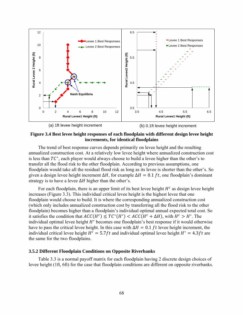
68

Figure 3.4 Best levee height responses of each floodplain with different design levee height increments, for identical floodplains

The trend of best response curves depends primarily on levee height and the resulting annualized construction cost. At a relatively low levee height where annualized construction cost is less than ∗, each player would always choose to build a levee higher than the other’s to transfer all the flood risk to the other floodplain. According to previous assumptions, one floodplain would take all the residual flood risk as long as its levee is shorter than the other’s. So given a design levee height increment ∆ , for example ∆ 0.1 , one floodplain’s dominant strategy is to have a levee ∆ higher than the other’s.

For each floodplain, there is an upper limit of its best levee height as design levee height increases (Figure 3.3). This individual critical levee height is the highest levee that one floodplain would choose to build. It is where the corresponding annualized construction cost (which only includes annualized construction cost by transferring all the flood risk to the other floodplain) becomes higher than a floodplain’s individual optimal annual expected total cost. So it satisfies the condition that ∗ ∗ ∆ , with ∗. The individual optimal levee height ∗ becomes one floodplain’s best response if it would otherwise have to pass the critical levee height. In this case with ∆ 0.1 levee height increment, the individual critical levee height 5.7 and individual optimal levee height ∗ 4.3 are the same for the two floodplains.

3.5.2 Different Floodplain Conditions on Opposite Riverbanks

Table 3.3 is a normal payoff matrix for each floodplain having 2 discrete design choices of levee height (1ft, 6ft) for the case that floodplain conditions are different on opposite riverbanks.

0

2

4

6

8

10

12

0 2 4 6 8 10 12

Ru

ral

Le

vee

2 H

eig

ht

(ft)

Rural Levee1 Height (ft)

Rural Levee1 BR

Rural Levee2 BR

3.5

4.5

5.5

6.5

3.5 4.5 5.5 6.5

Ru

ral L

eve

e2 H

eig

ht

(ft)

Rural Levee1 Height (ft)

Rural Levee1 BR

Rural Levee2 BR

(a) 1ft levee height increment (b) 0.1ft levee height increment

Levee 1 Best Responses

Levee 2 Best Responses

Levee 1 Best Responses

Levee 2 Best Responses

Nash Equilibria

69

Table 3.3 Payoffs for two floodplains with 1ft and 6ft design choices

Height of Urban Levee2 (ft)

1 6

Height of Rural Levee1 (ft)

1 0.89 2.13 1.72 0.56

6 0.56 4.20 0.60 0.66

The dominant strategies and Nash equilibrium (in bold) shown in Table 3.3 are similar to

those in Table 3.1. In this case, the best levee height for rural floodplain given 1ft high urban levee 2 is 6ft, and given 6ft high urban levee 2 is 6ft. Meanwhile, the best levee height for urban floodplain given 1ft high rural levee 1 is 6ft, and given 6ft high rural levee 1 is 6ft. And the dominant design levee height for rural floodplain or urban floodplain is 6ft, which results in a Nash equilibrium and also a social planner’s economically optimal levee system design.

Similar to Table 3.2, we have the following Table 3.4 showing the payoffs of two floodplains if each has 10 design choices of levee height from 1ft to 10ft with 1ft increment.

Table 3.4 Payoffs for two floodplains with 10 design choices

Height of Urban Levee2 (ft)

1 2 3 4 5 6 7 8 9 10

Height of

Rural Levee1 (ft)

1 0.89 2.13 1.72 0.15 1.72 0.23 1.72 0.33 1.72 0.44 1.72 0.56 1.72 0.69 1.72 0.83 1.72 0.98 1.72 1.14

2 0.15 4.20 0.55 1.15 0.95 0.23 0.95 0.33 0.95 0.44 0.95 0.56 0.95 0.69 0.95 0.83 0.95 0.98 0.95 1.14

3 0.23 4.20 0.23 2.15 0.43 0.73 0.63 0.33 0.63 0.44 0.63 0.56 0.63 0.69 0.63 0.83 0.63 0.98 0.63 1.14

4 0.33 4.20 0.33 2.15 0.33 1.24 0.44 0.60 0.54 0.44 0.54 0.56 0.54 0.69 0.54 0.83 0.54 0.98 0.54 1.14

5 0.44 4.20 0.44 2.15 0.44 1.24 0.44 0.86 0.50 0.59 0.56 0.56 0.56 0.69 0.56 0.83 0.56 0.98 0.56 1.14

6 0.56 4.20 0.56 2.15 0.56 1.24 0.56 0.86 0.56 0.75 0.60 0.66 0.64 0.69 0.64 0.83 0.64 0.98 0.64 1.14

7 0.69 4.20 0.69 2.15 0.69 1.24 0.69 0.86 0.69 0.75 0.69 0.76 0.72 0.76 0.75 0.83 0.75 0.98 0.75 1.14

8 0.83 4.20 0.83 2.15 0.83 1.24 0.83 0.86 0.83 0.75 0.83 0.76 0.83 0.83 0.85 0.89 0.88 0.98 0.88 1.14

9 0.98 4.20 0.98 2.15 0.98 1.24 0.98 0.86 0.98 0.75 0.98 0.76 0.98 0.83 0.98 0.95 1.00 1.03 1.02 1.14

10 1.14 4.20 1.14 2.15 1.14 1.24 1.14 0.86 1.14 0.75 1.14 0.76 1.14 0.83 1.14 0.95 1.14 1.08 1.16 1.19

Similarly, each floodplain would have a best design levee height for any anticipation of

another floodplain’s levee height. Unfortunately, this case has no Nash Equilibrium. A social planner’s economically optimal levee system design is a 3ft high rural levee 1 and a 4ft high urban levee 2, where all residual flood risk is transferred to the lower rural levee 1.

Figure 3.5(a) shows the best responses curves of each player with 1ft levee height increment. And Figure 3.5(b) is the best response curves with 0.1ft levee height increment within the more changing range of levee height between 4ft to 7.5ft. No Nash equilibrium exists with neither 1ft nor 0.1ft design levee height increment. And no Nash equilibrium exists with even

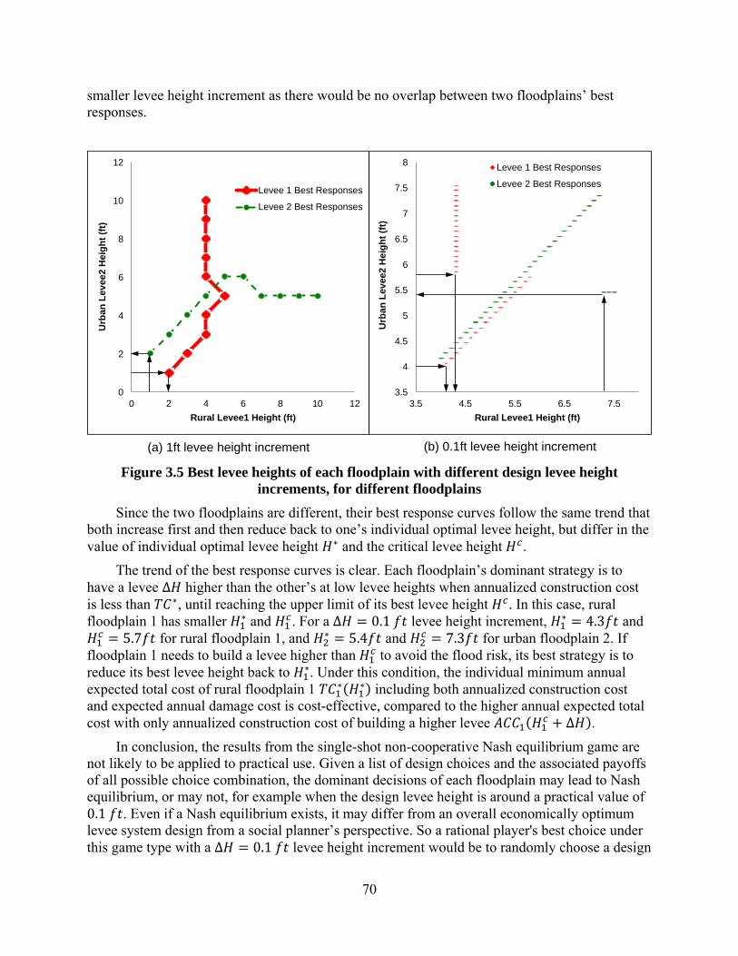
70

smaller levee height increment as there would be no overlap between two floodplains’ best responses.

Figure 3.5 Best levee heights of each floodplain with different design levee height increments, for different floodplains

Since the two floodplains are different, their best response curves follow the same trend that both increase first and then reduce back to one’s individual optimal levee height, but differ in the value of individual optimal levee height ∗ and the critical levee height .

The trend of the best response curves is clear. Each floodplain’s dominant strategy is to have a levee ∆ higher than the other’s at low levee heights when annualized construction cost is less than ∗, until reaching the upper limit of its best levee height . In this case, rural floodplain 1 has smaller ∗ and . For a ∆ 0.1 levee height increment, ∗ 4.3 and

5.7 for rural floodplain 1, and ∗ 5.4 and 7.3 for urban floodplain 2. If floodplain 1 needs to build a levee higher than to avoid the flood risk, its best strategy is to reduce its best levee height back to ∗. Under this condition, the individual minimum annual expected total cost of rural floodplain 1 ∗ ∗ including both annualized construction cost and expected annual damage cost is cost-effective, compared to the higher annual expected total cost with only annualized construction cost of building a higher levee ∆ .

In conclusion, the results from the single-shot non-cooperative Nash equilibrium game are not likely to be applied to practical use. Given a list of design choices and the associated payoffs of all possible choice combination, the dominant decisions of each floodplain may lead to Nash equilibrium, or may not, for example when the design levee height is around a practical value of 0.1 . Even if a Nash equilibrium exists, it may differ from an overall economically optimum levee system design from a social planner’s perspective. So a rational player's best choice under this game type with a ∆ 0.1 levee height increment would be to randomly choose a design

0

2

4

6

8

10

12

0 2 4 6 8 10 12

Urb

an L

evee

2 H

eig

ht

(ft)

Rural Levee1 Height (ft)

Rural Levee1 BR

Urban Levee2 BR

Levee 1 Best Responses

Levee 2 Best Responses

3.5

4

4.5

5

5.5

6

6.5

7

7.5

8

3.5 4.5 5.5 6.5 7.5

Urb

an L

evee

2 H

eig

ht

(ft)

Rural Levee1 Height (ft)

Rural Levee1 BR

Urban Levee2 BR

(a) 1ft levee height increment (b) 0.1ft levee height increment

Levee 1 Best Responses

Levee 2 Best Responses

71

levee height. Mixed strategies Nash equilibrium can help solving such randomness. But such a single-shot institutional situation for levee design would be highly unusual.

3.6 Successive Repeated Non-cooperative Game: Reversible Decision Making Mode

A repeated game in game theory includes multiple shots that a player can make moves (design decisions) at each shot step. The single shot game discussed above is non-repeated game (Osborne 1994). A repeated game involves the idea that a player has to account for the impacts from other players’ current and future actions. It is typically categorized into finitely and infinitely repeated games, depending on the number of times game repeated. An infinitely repeated game may keep growing as long as the possible strategies are infinite, or it could eventually follow a cycle or converge at some point (Fudenberg and Tirole 1991; Osborne 1994). Here the levee system design is examined as an infinitely repeated game, but we manually limit the number of steps game played when cycle or convergence is observed.

Levees have been served for flood control in California since the construction of the first levees in 1851, and there are inefficient competitive levee constructions in the early era (Hanak 2010). From 1867 to 1880, adjacent districts along the Sacramento River race each other to construct levees on each river bank (Russo 2010). In 1868, landowners along the Sacramento River and its tributaries were authorized to collaborate on flood control projects. Unfortunately, since channeled floodwater would overflow or breach shorter and weaker levees rather than taller and stronger levees, flood-prone landowners responded (in kind) to escalating their levees that essentially forced the floodwater onto their neighbors. The resulting continuous escalation of levees in the Sacramento Valley later became ineffective and economically inefficient, which may cause deliberate non-natural disasters during a flood that some landowners would demolish a neighbor’s levees instead of raising the height of their own levees (Kelley 1989).

In a repeated levee system design game that each floodplain can make levee construction decisions more than once, non-cooperative floodplains can change their best levee design strategies in response to the other in subsequent periods. This multi-shot levee system design game can involve reversible decisions, which is discussed in this section, or (more likely) irreversible decisions discussed in the next section (Smale 1980). We let each floodplain deciding their design levee heights initially from a lowest level. In a reversible game, each floodplain can choose all possible levee heights, even decrease heights back to its former choice, as its best design strategy at each step. However, in an irreversible game, each floodplain cannot decide to decrease its levee height, but can only increase its levee height by ∆ or make no change. Reinforcement-Learning (RL) (Sutten and Barto 2000) could be used to address this challenge and derive the best response strategies of non-cooperating players.

Assuming recurring levee system design decisions: before a final decision on design levee height, both floodplains can bargain over multiple times, until they reach converged heights or the allowed bargaining time ends. At each bargain step, one or both players would state its best design levee height at that time. Such successive multi-shot game can be either a leader-follower game or a simultaneous game. In a leader-follower game, one player as a leader starts the game and makes its best design decision at step 1. The other player as a follower makes its decision according to the leader’s decision at step 2, and this player in turn becomes the leader for step 3. Then in each of the following steps, the follower chooses its best decision according to the leader’s best decision from the previous step, and the follower at current step becomes the leader for next step. Whereas, in a simultaneous game, two players both make their best decisions at

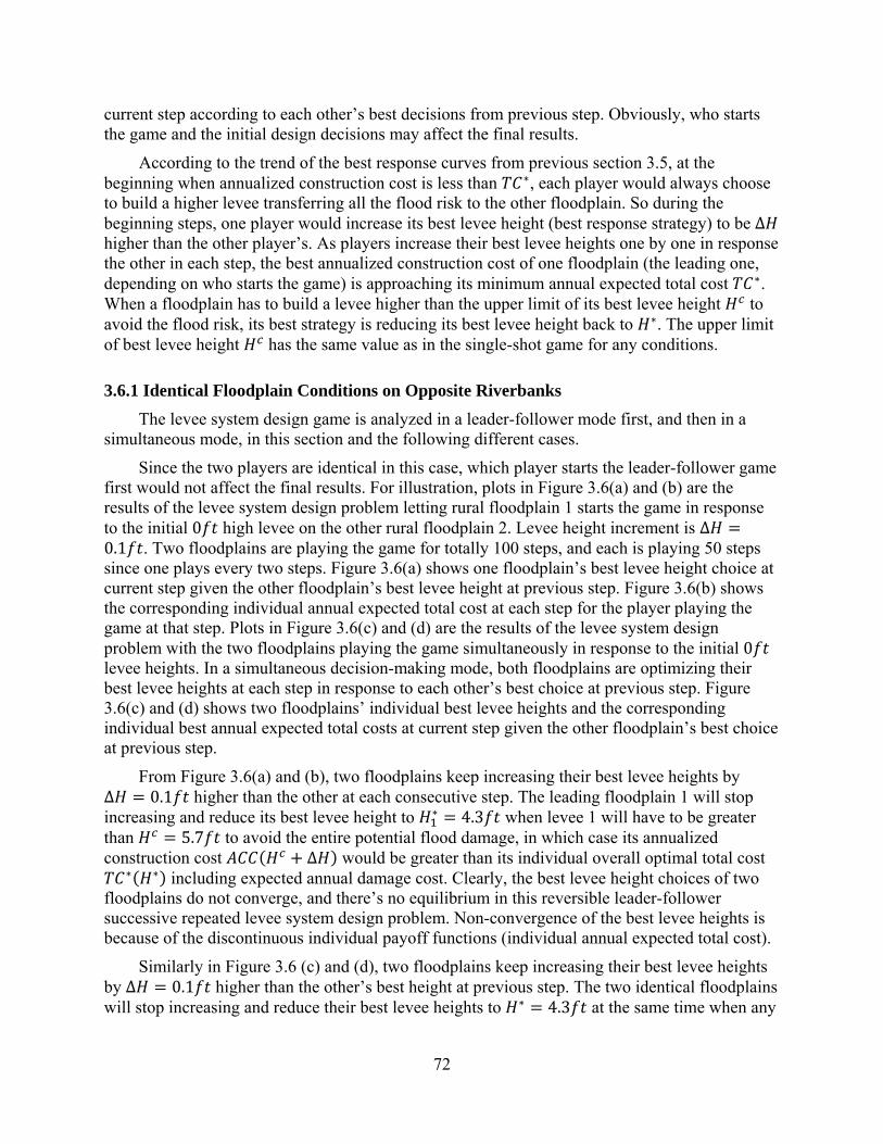
72

current step according to each other’s best decisions from previous step. Obviously, who starts the game and the initial design decisions may affect the final results.

According to the trend of the best response curves from previous section 3.5, at the beginning when annualized construction cost is less than ∗, each player would always choose to build a higher levee transferring all the flood risk to the other floodplain. So during the beginning steps, one player would increase its best levee height (best response strategy) to be ∆ higher than the other player’s. As players increase their best levee heights one by one in response the other in each step, the best annualized construction cost of one floodplain (the leading one, depending on who starts the game) is approaching its minimum annual expected total cost ∗. When a floodplain has to build a levee higher than the upper limit of its best levee height to avoid the flood risk, its best strategy is reducing its best levee height back to ∗. The upper limit of best levee height has the same value as in the single-shot game for any conditions.

3.6.1 Identical Floodplain Conditions on Opposite Riverbanks

The levee system design game is analyzed in a leader-follower mode first, and then in a simultaneous mode, in this section and the following different cases.

Since the two players are identical in this case, which player starts the leader-follower game first would not affect the final results. For illustration, plots in Figure 3.6(a) and (b) are the results of the levee system design problem letting rural floodplain 1 starts the game in response to the initial 0 high levee on the other rural floodplain 2. Levee height increment is ∆0.1 . Two floodplains are playing the game for totally 100 steps, and each is playing 50 steps since one plays every two steps. Figure 3.6(a) shows one floodplain’s best levee height choice at current step given the other floodplain’s best levee height at previous step. Figure 3.6(b) shows the corresponding individual annual expected total cost at each step for the player playing the game at that step. Plots in Figure 3.6(c) and (d) are the results of the levee system design problem with the two floodplains playing the game simultaneously in response to the initial 0 levee heights. In a simultaneous decision-making mode, both floodplains are optimizing their best levee heights at each step in response to each other’s best choice at previous step. Figure 3.6(c) and (d) shows two floodplains’ individual best levee heights and the corresponding individual best annual expected total costs at current step given the other floodplain’s best choice at previous step.

From Figure 3.6(a) and (b), two floodplains keep increasing their best levee heights by ∆ 0.1 higher than the other at each consecutive step. The leading floodplain 1 will stop increasing and reduce its best levee height to ∗ 4.3 when levee 1 will have to be greater than 5.7 to avoid the entire potential flood damage, in which case its annualized construction cost ∆ would be greater than its individual overall optimal total cost

∗ ∗ including expected annual damage cost. Clearly, the best levee height choices of two floodplains do not converge, and there’s no equilibrium in this reversible leader-follower successive repeated levee system design problem. Non-convergence of the best levee heights is because of the discontinuous individual payoff functions (individual annual expected total cost).

Similarly in Figure 3.6 (c) and (d), two floodplains keep increasing their best levee heights by ∆ 0.1 higher than the other’s best height at previous step. The two identical floodplains will stop increasing and reduce their best levee heights to ∗ 4.3 at the same time when any

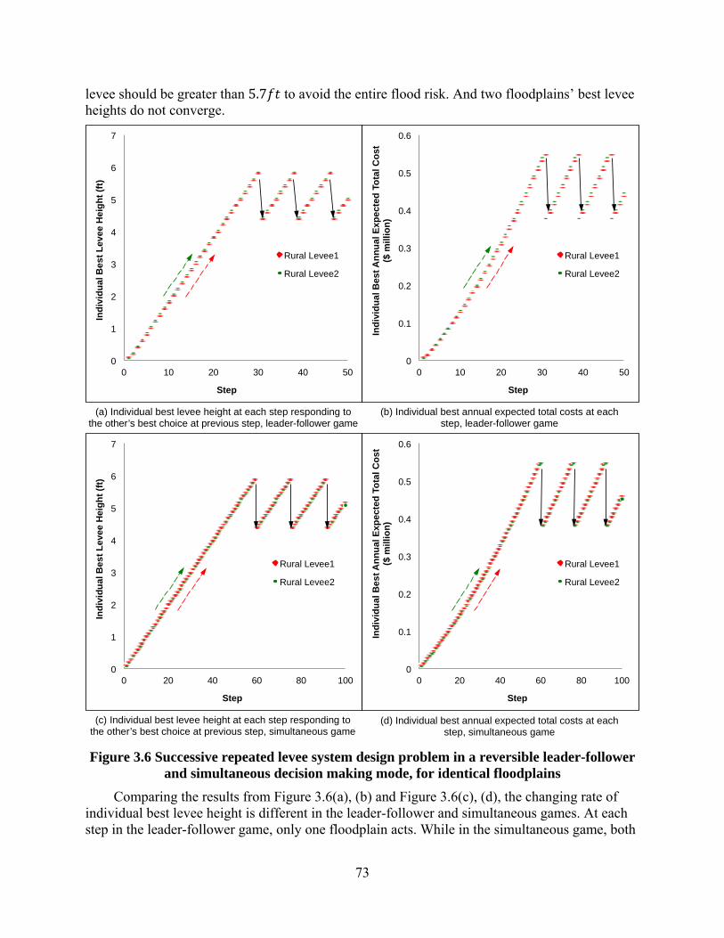
73

levee should be greater than 5.7 to avoid the entire flood risk. And two floodplains’ best levee heights do not converge.

Figure 3.6 Successive repeated levee system design problem in a reversible leader-follower and simultaneous decision making mode, for identical floodplains

Comparing the results from Figure 3.6(a), (b) and Figure 3.6(c), (d), the changing rate of individual best levee height is different in the leader-follower and simultaneous games. At each step in the leader-follower game, only one floodplain acts. While in the simultaneous game, both

0

1

2

3

4

5

6

7

0 10 20 30 40 50

Ind

ivid

ual

Be

st L

evee

Hei

gh

t (f

t)

Step

Rural Levee1

Rural Levee2

0

0.1

0.2

0.3

0.4

0.5

0.6

0 10 20 30 40 50 In

div

idu

al B

est

An

nu

al E

xpe

cted

To

tal C

ost

($

mill

ion

) Step

Rural Levee1

Rural Levee2

(a) Individual best levee height at each step responding to the other’s best choice at previous step, leader-follower game

(b) Individual best annual expected total costs at each step, leader-follower game

0

1

2

3

4

5

6

7

0 20 40 60 80 100

Ind

ivid

ual

Bes

t L

evee

Hei

gh

t (f

t)

Step

Rural Levee1

Rural Levee2

0

0.1

0.2

0.3

0.4

0.5

0.6

0 20 40 60 80 100

Ind

ivid

ual

Bes

t A

nn

ual

Exp

ecte

d T

ota

l Co

st

($ m

illio

n)

Step

Rural Levee1

Rural Levee2

(d) Individual best annual expected total costs at each step, simultaneous game

(c) Individual best levee height at each step responding to the other’s best choice at previous step, simultaneous game

74

floodplains play the game at each step. Besides, one floodplain’s best levee height always increases by ∆ 0.1 than the other’s previous best height, if not decreases. So the individual best levee height of each floodplain is increasing by 2∆ at its two consecutive steps in the leader-follower game, while by ∆ at its two consecutive steps in the simultaneous game. Since the unstable tie condition is avoided and decision making is more efficient, the resulting best levee height increases two times faster when two floodplains acting as leader and follower. This is also shown in the later comparison between leader and follower case and simultaneous case for different floodplain conditions. Another difference is the resulting individual best levee heights of two floodplains at the given step where they have to stop the game, even there’s no convergence. Two floodplains’ final individual best levee heights are the same in the simultaneous game, while there is a ∆ difference in the leader-follower game.

We also could draw best response curves for the above results, which are the same for the leader-follower game and the simultaneous game. Figure 3.7(a) shows the best responses of each floodplain within the possible choices region, from the initial 0 to the upper limit of the best levee height 5.7 . To show the dynamic of the best responses, Figure 3.7(b) shows the trends of the best response curves that each individual floodplain’s best design levee heights are clearly trapped following a cycle (best responses for levee heights from 3 to 5.7 ). The non-convergence and lack of equilibrium in this reversible successive repeated levee system design problem are seen in Figure 3.7(b). This case of best responses eventually following a cycle is similar to the typical rock-paper-scissors game, but with more strategies (Fisher 2008).

Figure 3.7 Best response curves in the successive repeated levee system design problem in a reversible decision making mode, for identical floodplains

3.6.2 Different Floodplain Conditions on Opposite Riverbanks

When floodplain conditions are different on opposite riverbanks, which player starts first may affect the final results. So the 100-step game is played twice, letting each floodplain starts

(a) Best Response Curves within feasible region (b) Best Response Curves trends

0

1

2

3

4

5

6

7

0 1 2 3 4 5 6 7

Ru

ral

Le

vee2

Hei

gh

t (f

t)

Rural Levee1 Height (ft)

Rural Levee1 BR

Rural Levee2 BR

3

3.5

4

4.5

5

5.5

6

3 3.5 4 4.5 5 5.5 6

Ru

ral

Le

vee2

Hei

gh

t (f

t)

Rural Levee1 Height (ft)

Rural Levee1 BR

Rural Levee2 BR

Levee 1 Best Responses

Levee 2 Best Responses

(b)

Levee 1 Best Responses

Levee 2 Best Responses

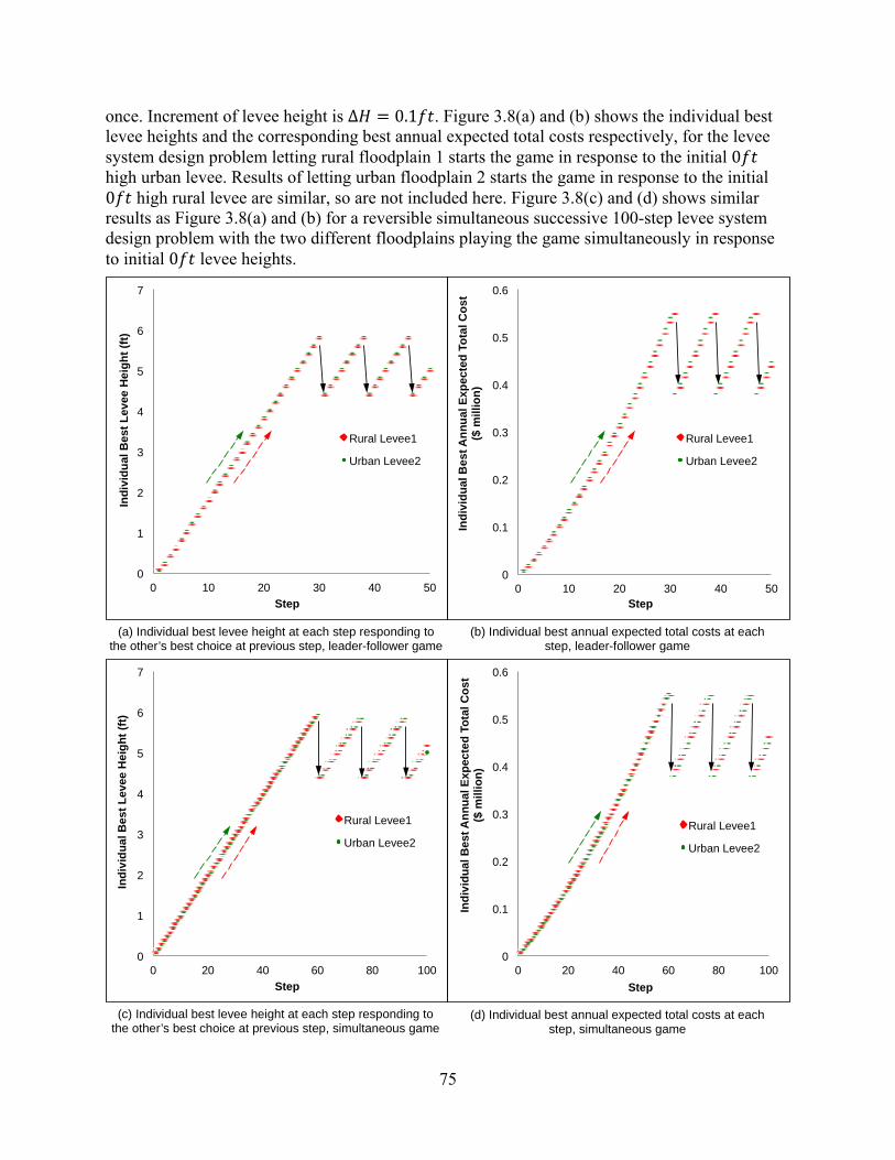
75

once. Increment of levee height is ∆ 0.1 . Figure 3.8(a) and (b) shows the individual best levee heights and the corresponding best annual expected total costs respectively, for the levee system design problem letting rural floodplain 1 starts the game in response to the initial 0 high urban levee. Results of letting urban floodplain 2 starts the game in response to the initial 0 high rural levee are similar, so are not included here. Figure 3.8(c) and (d) shows similar results as Figure 3.8(a) and (b) for a reversible simultaneous successive 100-step levee system design problem with the two different floodplains playing the game simultaneously in response to initial 0 levee heights.

0

1

2

3

4

5

6

7

0 10 20 30 40 50

Ind

ivid

ual

Bes

t L

evee

He

igh

t (f

t)

Step

Rural Levee1

Urban Levee2

0

0.1

0.2

0.3

0.4

0.5

0.6

0 10 20 30 40 50

Ind

ivid

ual

Bes

t A

nn

ual

Exp

ecte

d T

ota

l Co

st

($ m

illio

n)

Step

Rural Levee1

Urban Levee2

(a) Individual best levee height at each step responding to the other’s best choice at previous step, leader-follower game

(b) Individual best annual expected total costs at each step, leader-follower game

0

1

2

3

4

5

6

7

0 20 40 60 80 100

Ind

ivid

ual

Bes

t L

evee

He

igh

t (f

t)

Step

Rural Levee1

Urban Levee2

0

0.1

0.2

0.3

0.4

0.5

0.6

0 20 40 60 80 100

Ind

ivid

ua

l Bes

t A

nn

ual

Exp

ecte

d T

ota

l C

os

t

($

mill

ion

)

Step

Rural Levee1

Urban Levee2

(d) Individual best annual expected total costs at each step, simultaneous game

(c) Individual best levee height at each step responding to the other’s best choice at previous step, simultaneous game

76

Figure 3.8 Successive repeated levee system design problem in a reversible leader-follower and simultaneous decision making mode, for different floodplains

Results shown in Figure 3.8 are similar to those in Figure 3.6. The two floodplains keep increasing their best levee heights by ∆ 0.1 higher than the other’s height at previous step. Floodplain 1 in the less damageable rural area will stop increasing and reduce its best levee height to ∗ 4.3 when levee 1 should be greater than 5.7 to avoid the entire potential flood damage. The levee heights do not convergence and no equilibrium exists in this reversible leader-follower successive multi-shot levee system design game.

An interesting result in this multi-shot game is that after the first jumping down from the peaks, levee 1 is always ∆ higher than levee 2 at each step, except for when levee 1 is at its bottom best height of ∗ 4.3 . This is because that starting from the bottom where floodplain 1 choses ∗ 4.3 and floodplain 2 chooses ∗ ∆ , best responses to each other’s previous best height would lead to floodplain 1 being ∆ higher than floodplain 2 in the following steps till the peak.

The best response curves for the above results are plotted in Figure 3.9, (a) for the leader-follower game and (b) for the simultaneous game. Similar to the best response curves trends in Figure 3.7, each individual floodplain’s best design levee heights are trapped following a cycle, but different floodplains follow different cycles in theory. Since two floodplains make decisions in response to each other, Figure 3.9(b) shows the real best responses curves that rural floodplain 1 follows a cycle and urban floodplain 2 follows a line back and forth as following floodplain 1’s cycle by one step behind. There is still non-convergence and no equilibrium in this reversible successive multi-shot levee system design problem.

Figure 3.9 Best response curves in the successive repeated levee system design problem in a reversible decision making mode, for different floodplains

(a) Possible Best Response Curves trends (Leader & Follower case)

(b) Actual Best Response Curves trends (Simultaneous case)

3.5

4

4.5

5

5.5

6

6.5

7

7.5

3.5 4.5 5.5 6.5 7.5

Urb

an L

eve

e2

Hei

gh

t (f

t)

Rural Levee1 Height (ft)

Rural Levee1 BR

Urban Levee2 BR 3

3.5

4

4.5

5

5.5

6

3 3.5 4 4.5 5 5.5 6

Urb

an L

eve

e2

Hei

gh

t (f

t)

Rural Levee1 Height (ft)

Rural Levee1 BR

Urban Levee2 BR

Levee 1 Best Responses

Levee 2 Best Responses

Levee 1 Best Responses

Levee 2 Best Responses

Levee 2 fo

llows L

evee 1’s

cycle

by one st

ep behind

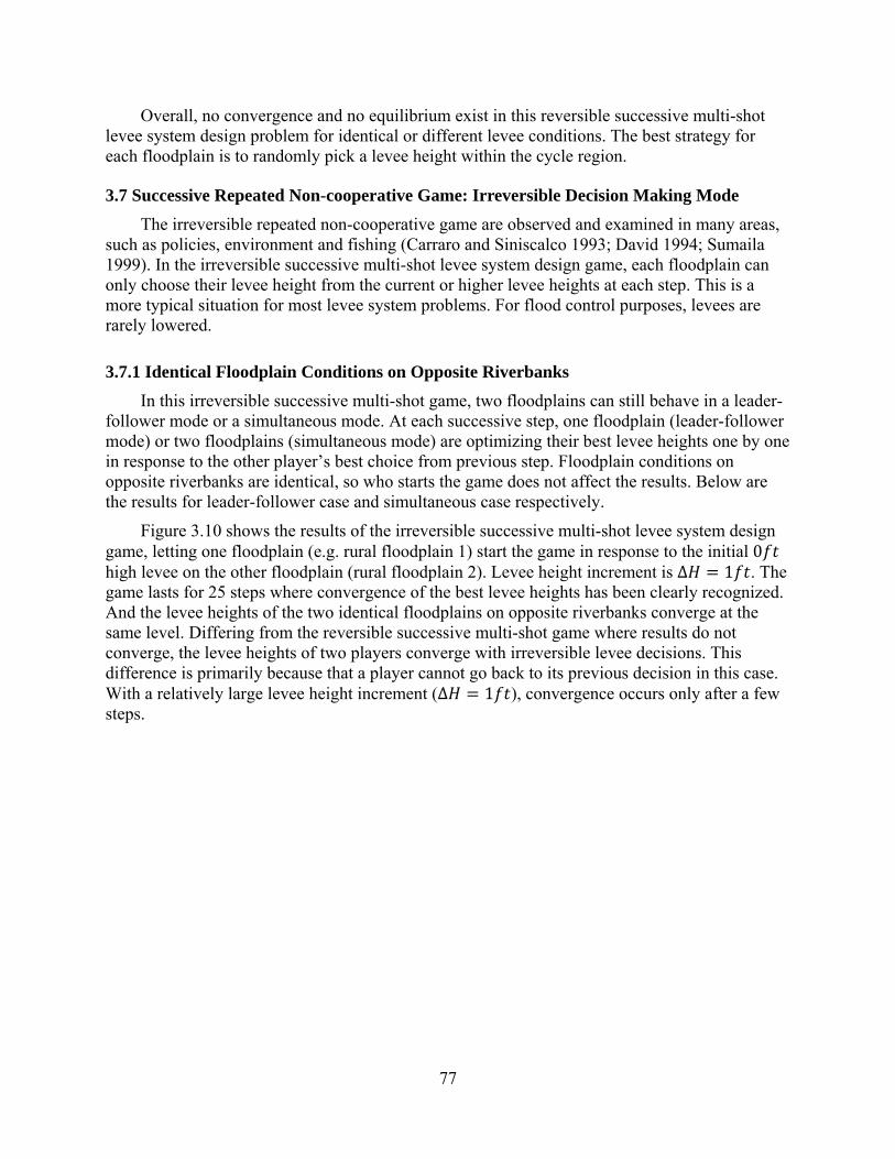
77

Overall, no convergence and no equilibrium exist in this reversible successive multi-shot levee system design problem for identical or different levee conditions. The best strategy for each floodplain is to randomly pick a levee height within the cycle region.

3.7 Successive Repeated Non-cooperative Game: Irreversible Decision Making Mode

The irreversible repeated non-cooperative game are observed and examined in many areas, such as policies, environment and fishing (Carraro and Siniscalco 1993; David 1994; Sumaila 1999). In the irreversible successive multi-shot levee system design game, each floodplain can only choose their levee height from the current or higher levee heights at each step. This is a more typical situation for most levee system problems. For flood control purposes, levees are rarely lowered.

3.7.1 Identical Floodplain Conditions on Opposite Riverbanks

In this irreversible successive multi-shot game, two floodplains can still behave in a leader-follower mode or a simultaneous mode. At each successive step, one floodplain (leader-follower mode) or two floodplains (simultaneous mode) are optimizing their best levee heights one by one in response to the other player’s best choice from previous step. Floodplain conditions on opposite riverbanks are identical, so who starts the game does not affect the results. Below are the results for leader-follower case and simultaneous case respectively.

Figure 3.10 shows the results of the irreversible successive multi-shot levee system design game, letting one floodplain (e.g. rural floodplain 1) start the game in response to the initial 0 high levee on the other floodplain (rural floodplain 2). Levee height increment is ∆ 1 . The game lasts for 25 steps where convergence of the best levee heights has been clearly recognized. And the levee heights of the two identical floodplains on opposite riverbanks converge at the same level. Differing from the reversible successive multi-shot game where results do not converge, the levee heights of two players converge with irreversible levee decisions. This difference is primarily because that a player cannot go back to its previous decision in this case. With a relatively large levee height increment (∆ 1 ), convergence occurs only after a few steps.

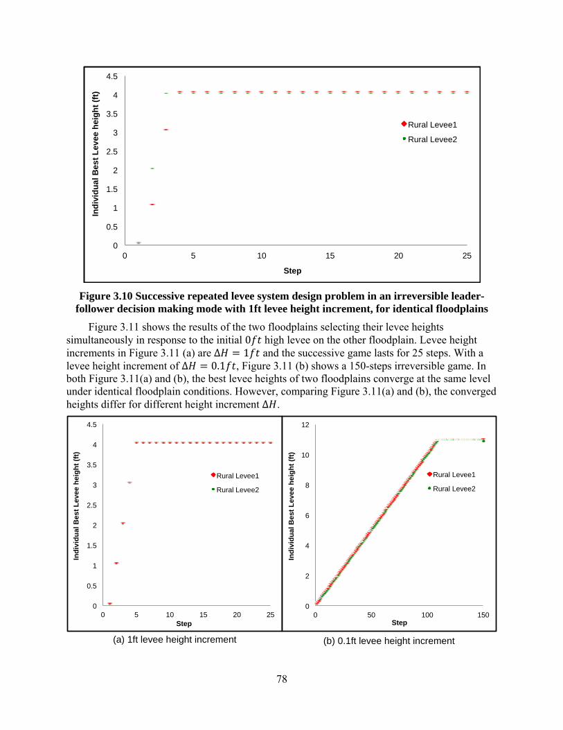
78

Figure 3.10 Successive repeated levee system design problem in an irreversible leader-follower decision making mode with 1ft levee height increment, for identical floodplains

Figure 3.11 shows the results of the two floodplains selecting their levee heights simultaneously in response to the initial 0 high levee on the other floodplain. Levee height increments in Figure 3.11 (a) are ∆ 1 and the successive game lasts for 25 steps. With a levee height increment of ∆ 0.1 , Figure 3.11 (b) shows a 150-steps irreversible game. In both Figure 3.11(a) and (b), the best levee heights of two floodplains converge at the same level under identical floodplain conditions. However, comparing Figure 3.11(a) and (b), the converged heights differ for different height increment ∆ .

0

0.5

1

1.5

2

2.5

3

3.5

4

4.5

0 5 10 15 20 25

Ind

ivid

ua

l Bes

t L

evee

hei

gh

t (f

t)

Step

Rural Levee1

Rural Levee2

0

0.5

1

1.5

2

2.5

3

3.5

4

4.5

0 5 10 15 20 25

Ind

ivid

ual

Bes

t L

evee

hei

gh

t (f

t)

Step

Rural Levee1

Rural Levee2

(a) 1ft levee height increment

0

2

4

6

8

10

12

0 50 100 150

Ind

ivid

ual

Bes

t L

evee

hei

gh

t (f

t)

Step

Rural Levee1

Rural Levee2

(b) 0.1ft levee height increment

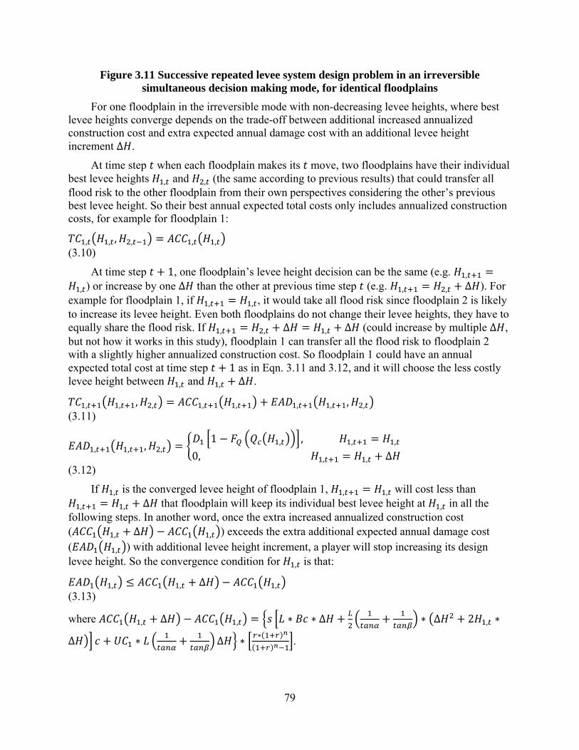
79

Figure 3.11 Successive repeated levee system design problem in an irreversible simultaneous decision making mode, for identical floodplains

For one floodplain in the irreversible mode with non-decreasing levee heights, where best levee heights converge depends on the trade-off between additional increased annualized construction cost and extra expected annual damage cost with an additional levee height increment ∆ .

At time step when each floodplain makes its move, two floodplains have their individual best levee heights , and , (the same according to previous results) that could transfer all flood risk to the other floodplain from their own perspectives considering the other’s previous best levee height. So their best annual expected total costs only includes annualized construction costs, for example for floodplain 1:

, , , , , , (3.10)

At time step 1, one floodplain’s levee height decision can be the same (e.g. ,

, ) or increase by one ∆ than the other at previous time step (e.g. , , ∆ ). For example for floodplain 1, if , , , it would take all flood risk since floodplain 2 is likely to increase its levee height. Even both floodplains do not change their levee heights, they have to equally share the flood risk. If , , ∆ , ∆ (could increase by multiple ∆ , but not how it works in this study), floodplain 1 can transfer all the flood risk to floodplain 2 with a slightly higher annualized construction cost. So floodplain 1 could have an annual expected total cost at time step 1 as in Eqn. 3.11 and 3.12, and it will choose the less costly levee height between , and , ∆ .

, , , , , , , , , , (3.11)

, , , ,1 , , , ,

0, , , ∆

(3.12)

If , is the converged levee height of floodplain 1, , , will cost less than

, , ∆ that floodplain will keep its individual best levee height at , in all the following steps. In another word, once the extra increased annualized construction cost ( , ∆ , ) exceeds the extra additional expected annual damage cost ( , ) with additional levee height increment, a player will stop increasing its design levee height. So the convergence condition for , is that:

, , ∆ , (3.13)

where , ∆ , ∗ ∗ ∆ ∗ ∆ 2 , ∗

∆ ∗ ∆ ∗ ∗.

80

Decreasing ∆ will decrease , ∆ , , while , decreases as , increases, although there is a slight counteraction from , on annualized construction cost (Figure 3.3). So a smaller ∆ will lead to slightly larger converged best levee heights. This could be shown mathematically by substituting the formula of and from Eqn. 3.5 and 3.6 to Eqn. 3.13. Theoretically without any limitations on levee construction, if the levee height increment ∆ is infinitely small, the converged best levee heights will be infinitely large. But such situation is most unlikely in reality due to the design standards for levee height increments and financial budget limit for possible costs, and most importantly the upper limit of standard design levee height.

3.7.2 Different Floodplain Conditions on Opposite Riverbanks

With different floodplain conditions on opposite riverbanks, which floodplain starts the leader-follower game may affect the results. However, in this irreversible successive levee system design game, the results are similar for regardless floodplain starts. For illustration, Figure 3.12 shows the results of letting rural floodplain 1 start first in response to the initial 0 high levee on urban floodplain 2. Design levee height increment is ∆ 1 and the game is lasting for 25 steps. Similar to the results in Figure 3.10 for identical floodplain conditions, best levee heights of two players converge after a few number of steps. The difference between the two converged best levee heights is one levee height increment (∆ 1 ) in this case.

Figure 3.12 Successive repeated levee system design problem in an irreversible leader-follower decision making mode with 1ft levee height increment, for different floodplains

Similar to Figure 3.11, Figure 3.13 shows the results of the irreversible levee system design problem with the two floodplains playing the game simultaneously in response to the initial 0 levee heights. Levee height increment in Figure 3.12 (a) is ∆ 1 with the game lasting for 25 steps, and in Figure 3.13 (b) is ∆ 0.1 with the game lasting for 150 steps. Individual best levee height converges after a number of steps for each floodplain, while converged heights differ for two different floodplains in this case. For either 1ft levee height increment in Figure 3.13(a) or 0.1ft levee height increment in Figure 3.13(b), the difference between the two

0

1

2

3

4

5

6

7

0 5 10 15 20 25

Ind

ivid

ual

Bes

t L

evee

hei

gh

t (f

t)

Step

Rural Levee1

Urban Levee2

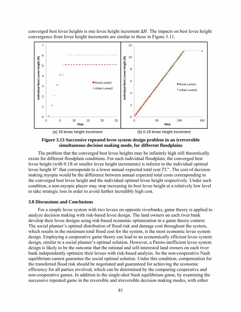
81

converged best levee heights is one levee height increment ∆ . The impacts on best levee height convergence from levee height increments are similar to those in Figure 3.11.

Figure 3.13 Successive repeated levee system design problem in an irreversible simultaneous decision making mode, for different floodplains

The problem that the converged best levee heights may be infinitely high still theoretically exists for different floodplain conditions. For each individual floodplain, the converged best levee height (with 0.1ft or smaller levee height increments) is inferior to the individual optimal levee height ∗ that corresponds to a lower annual expected total cost ∗. The cost of decision making myopia would be the difference between annual expected total costs corresponding to the converged best levee height and the individual optimal levee height respectively. Under such condition, a non-myopic player may stop increasing its best levee height at a relatively low level to take strategic loss in order to avoid further incredibly high cost.

3.8 Discussions and Conclusions

For a simple levee system with two levees on opposite riverbanks, game theory is applied to analyze decision making with risk-based levee design. The land owners on each river bank develop their levee designs using risk-based economic optimization in a game theory context. The social planner’s optimal distribution of flood risk and damage cost throughout the system, which results in the minimum total flood cost for the system, is the most economic levee system design. Employing a cooperative game theory can lead to an economically efficient levee system design, similar to a social planner’s optimal solution. However, a Pareto-inefficient levee system design is likely to be the outcome that the rational and self-interested land owners on each river bank independently optimize their levees with risk-based analysis. So the non-cooperative Nash equilibrium cannot guarantee the social optimal solution. Under this condition, compensation for the transferred flood risk should be negotiated and guaranteed for achieving the economic efficiency for all parties involved, which can be determined by the comparing cooperative and non-cooperative games. In addition to the single-shot Nash equilibrium game, by examining the successive repeated game in the reversible and irreversible decision making modes, with either

(a) 1ft levee height increment (b) 0.1ft levee height increment

0

1

2

3

4

5

6

7

0 5 10 15 20 25

Ind

ivid

ual

Bes

t L

evee

hei

gh

t (f

t)

Step

Rural Levee1

Urban Levee2

0

2

4

6

8

10

12

0 50 100 150 In

div

idu

al B

est

Lev

ee h

eig

ht

(ft)

Step

Rural Levee1

Urban Levee2

82

identical or different floodplain conditions on opposite riverbanks, problems of non-convergence and no equilibria are identified and the cost of decision making myopia is calculated to show the significance of externalities and evolution of dynamic water resource problems for optimal decision making.

Conclusions of this levee system design study are: (1) a social planner is necessary that can guarantee an economically efficient levee system design in all cases; (2) a rational land owner may become trapped in a cycle or accepting unreasonable decisions in some cases; (3) random choice is the best in some cases; and (4) strategic loss could avoid further incredibly high cost if a player is not myopic.

Furture study on this levee system design problem can analyze how the structure of this game evolves over time, and how the resulting equilibriums and the Pareto-optimal outcomes of the game change. Similar game theory can be applied to complex levee systems that involve multiple players, for example in a ring levee system that each player is in charge of one levee section, to predict the different behaviors of each individual player and coalitions.

3.9 References

Brandenburger, A. (2007). Cooperative game theory: Characteristic functions, allocations, marginal contribution. Stern School of Business. New York University.

Carraro, C., & Siniscalco, D. (1993). Strategies for the international protection of the environment. Journal of public Economics, 52(3), 309-328.

Carraro, C., Marchiori, C., & Sgobbi, A. (2005). Applications of negotiation theory to water issues (Vol. 3641). World Bank Publications.

Colman, A. M. (2013). Game theory and its applications: in the social and biological sciences. Psychology Press.

Croghan, L. (2013). Economic Model for Optimal Flood Risk Transfer. Master’s Thesis. David, P. A. (1994). Why are institutions the ‘carriers of history’?: Path dependence and the

evolution of conventions, organizations and institutions. Structural change and economic dynamics, 5(2), 205-220.

Fisher, L. (2008). Rock, paper, scissors: game theory in everyday life. Basic Books. Fudenberg, D., & Tirole, J. (1991). Game theory, 1991. Cambridge, Massachusetts. Gibbons, R. (1992). A primer in game theory. Hanak, E. (2011). Managing California's water: From conflict to reconciliation. Public Policy

Instit. of CA. Hashimoto, T., J. R. Stedinger, and D. P. Loucks (1982), Reliability, resiliency, and vulnerability

criteria for water resource system performance evaluation, Water Resour. Res., 18(1), 14–20.

Kelley, R. (1989). Battling the Inland Sea: Floods, Public Policy and the Sacramento River. Univ. of Cal. Press: Berkeley, CA.

Lund, J. R., & Palmer, R. N. (1997). Water resource system modeling for conflict resolution. Water Resources Update, 3(108), 70-82.

Lund, J. R. (2012). Flood management in California. Water, 4(1), 157-169. Madani, K. (2010). Game theory and water resources. Journal of Hydrology, 381(3), 225-238. Nash, J. (1951). Non-cooperative games. Annals of mathematics, 286-295. Nash, J. (1953). Two-person cooperative games. Econometrica: Journal of the Econometric

Society, 128-140.

83

Neumann, L. J., & Morgenstern, O. (1947). Theory of games and economic behavior (Vol. 60). Princeton, NJ: Princeton university press.

Osborne, M. J., & Rubinstein, A. (1994). A course in game theory. MIT press. Ostrom, E. (1998). A behavioral approach to the rational choice theory of collective action:

Presidential address, American Political Science Association, 1997. American Political Science Review, 1-22.

Parrachino, I., Dinar, A., & Patrone, F. (2006). Cooperative game theory and its application to natural, environmental, and water resource issues: 3. application to water resources. Application to Water Resources (November 2006). World Bank Policy Research Working Paper, (4074).

Russo, M. (2010). Fact Sheet, Sacramento River Flood Control System Weirs and Flood Relief Structures. State of California, The Resources Agency, Department of Water Resources, Division of Flood Management, Flood Operations Branch

Smale, S. (1980). The prisoner's dilemma and dynamical systems associated to non-cooperative games. Econometrica: Journal of the Econometric Society, 1617-1634.

Sumaila, U. R. (1999). A review of game-theoretic models of fishing. Marine policy, 23(1), 1-10. Tung, Y.-K., and L. W. Mays (1981a), Risk models for flood levee design, Water Resour. Res.,

17(4), 833–841. Tung, Y.-K., and L. W. Mays (1981b), Optimal risk-based design of flood levee systems, Water

Resour. Res., 17(4), 843–852. USACE (2006), TL 1110-2-561, Reliability Analysis and Risk Assessment for Seepage and

Slope Stability Failure Modes for Embankment Dams. Van Dantzig, D. (1956). Economic decision problems for flood prevention. Econometrica:

Journal of the Econometric Society, 276-287. Wolf, A. T. (2002). Conflict prevention and resolution in water systems. Edward Elgar

Publishing Ltd. Zara, S., Dinar, A., & Patrone, F. (2006). Cooperative game theory and its application to natural,

environmental, and water resource issues: 2. application to natural and environmental resources. Application to Natural and Environmental Resources (November 1, 2006). World Bank Policy Research Working Paper, (4073).

84

Chapter 4: Optimal Flood Pre-release—flood hedging for a single reservoir

4.1 Summary

Flood hedging reservoir operation is when a pre-storm release creates a small flood downstream (with certainty) to reduce the likelihood of a larger more damaging flood in the future. Such pre-releases before a storm can increase reservoir storage capacity available to capture severe flood volumes, but also can increase downstream levee failure risks and reduce stored water supply. This paper explores some theoretical conditions needed for flood hedging to be optimal, considering the hydrologic uncertainty from flood forecast and engineering uncertainty from levee overtopping and internal structural failures. Forecasted storms are categorized as small, intermediate or overwhelmingly large, depending on flood risk likelihood downstream. Extremely large storms, which overwhelm flood management systems, and small storms, which are handled relatively easily, do not encourage flood hedging operations. Intermediate storms that are large, but not overwhelming, where additional flood storage capacity from pre-releases materially reduces overall flood damage, drives the optimality of flood hedging pre-release operations. The ideal theoretical condition for optimal flood hedging is that current marginal damages from pre-releases equal future marginal expected damages from later storm releases. A necessary condition for flood hedging is that the overall risk from flood pre-release decisions are convex. The convexity in overall flood risk works with the probability distribution of possible storms to determine the optimality of flood hedging. Water supply losses due to pre-releases tend to reduce the use of hedging pre-release for flood management.

4.2 Introduction

“Life is uncertain. Eat dessert first.”

Ernestine Ulmer, 1892-1987

Flood protection is a major function of most large reservoirs. Many simulation and optimization models have been developed for release decisions to reduce potential flood damages (Wurbs 1993; Lund 2002; Labadie 2004). Operating rules based on flood-storage levels often are used for reservoir release decisions during flood seasons (Stedinger 1997). For flood operation, reservoirs sometimes encounter a situation where water is stored in the reservoir and a large oncoming flood is forecast. So the operating agency can release water from the reservoir in advance of the storm to make space for a likely major flood. In some cases, it might be worthwhile to make a large pre-release, which causes small downstream flood losses (sometimes with certainty), but lowers the probability of much larger oncoming flood damages. This situation of a trade-off between current and future probable flood damages is similar to water supply hedging for current and future water use benefits (Zhao et al. 2014).

In water supply reservoir operations, hedging involves creating a small water shortage in the near term as a way to reduce the probability of large shortages in the future (Draper and Lund 2004; You and Cai 2008a; Zhao et al. 2011). Water supply hedging deals with the trade-off between current and future benefits from water uses for limited water availability. For water supply hedging to be optimal, a necessary condition is that a large shortage be disproportionately

85

more costly than a small shortage, and there must be significant persistence or length to dry periods (Draper and Lund 2004).

Hedging rules for water supply have been derived with numerical optimization methods and hydroeconomic analysis. Studies on water supply hedging have improved the understanding of creating small current water shortages in case of likely future large water shortages, and strengthened the practical optimal operation rules by incorporating hydrologic uncertainties and real engineering constraints (Draper and Lund 2004; You and Cai 2008a, b; Shiau 2011; Zhao et al. 2011). The fundamental rational hedging is when the marginal expected benefit of storing water equals that of releasing water (Draper and Lund 2004). You and Cai (2008a, b) implemented economic and numerical analyses for hedging rules considering the uncertain future inflow. Shiau (2011) analyzed the hedging rules for the beneficial balances between current release and carry-over storage. Zhao et al. (2011) interpreted economically the typical physical constraints in water supply hedging.

Zhao et al. (2014) discussed the similarities between flood hedging rules and water supply hedging rules, and pointed out some dissimilarities between water supply and flood operation problems. The basic principle of flood hedging for a single storm is to equalize the marginal expected costs of current and future damage by allocating the expected flood-safety margin between expected flood volume and flood-conveyance capacity.

Former hedging studies (You and Cai 2008a, b; Zhao et al. 2011; Zhao et al. 2014) focused on hydrologic uncertainty only. Zhao et al. (2014) assumes that flood risk is only from levee overtopping, ignoring the frequently observed levee internal structural failures. Such engineering uncertainty from different levee failure modes, should also be incorporated into hedging analysis for levee systems in general conditions.

This study analytically examines flood hedging for one oncoming flood to a single reservoir from theoretical perspective. Hydrologic uncertainty is usually represented as an ensemble of possible forecasted storms for one future flood event. A simple model is developed to determine the optimal flood hedging pre-release by minimizing the expected flood damages from the range of forecasted storms over the current and forecast periods. The section proceeds as follows. Section 4.3 introduces a basic optimization model for determining the best flood hedging pre-release. Different failure probability curves and storms in different sizes are briefly discussed. Section 4.4 derives the theoretical optimal conditions for this optimization model, including Lagrange Multiplier and KKT conditions, theoretical optima for general levee failure probability curves, and some apparent implications from the theoretical optima. Section 4.5 shows the application of this model by discussing and comparing two illustrative examples for different failure probability functions, and demonstrates the theoretical optimal conditions. Section 4.6 extends the optimization formulation by incorporating additional economic water supply losses from spilled pre-releases, and by merging water supply hedging with flood hedging to develop blended hedging rules. Section 4.7 concludes this paper.

4.3 Simple Optimization Formulation

4.3.1 Model Description

Consider the case of a simple reservoir with a capacity , protecting a leveed downstream town (Figure 4.1). The levee protecting the town could fail by overtopping failure or internal

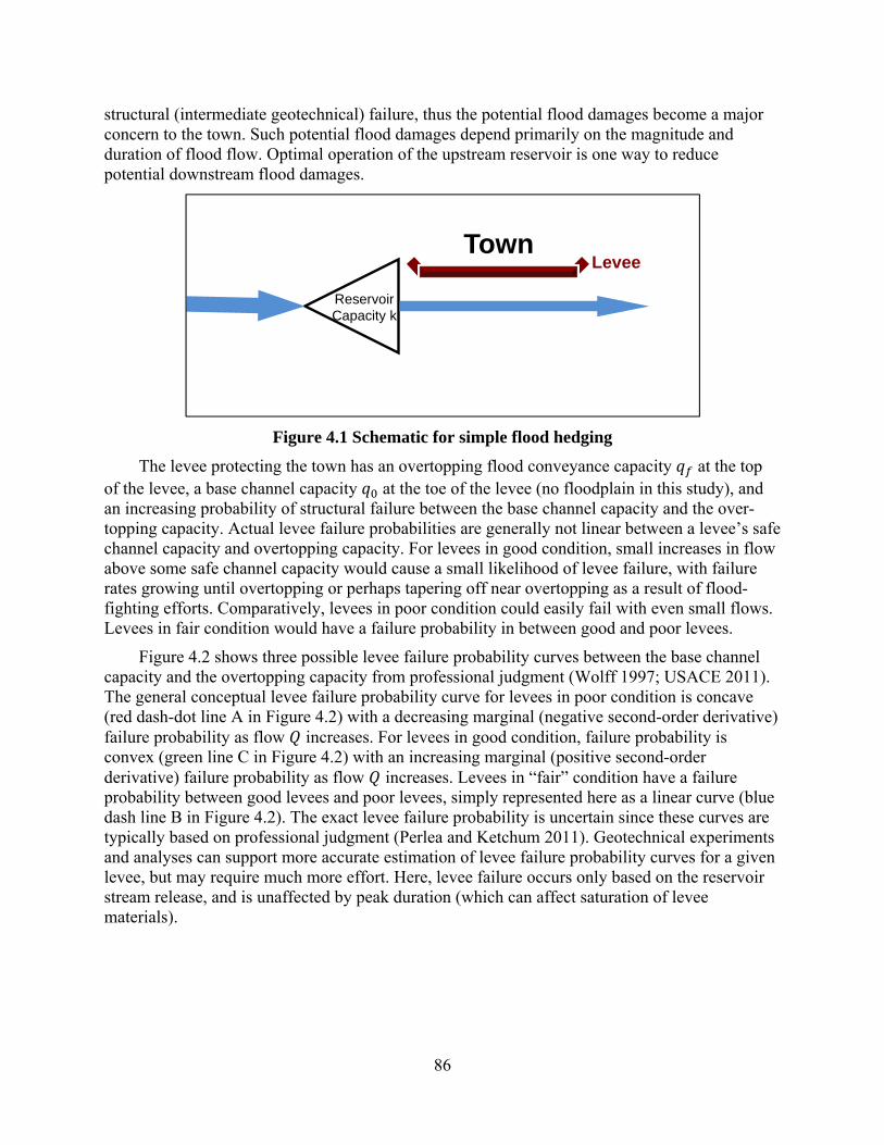
86

structural (intermediate geotechnical) failure, thus the potential flood damages become a major concern to the town. Such potential flood damages depend primarily on the magnitude and duration of flood flow. Optimal operation of the upstream reservoir is one way to reduce potential downstream flood damages.

Figure 4.1 Schematic for simple flood hedging

The levee protecting the town has an overtopping flood conveyance capacity at the top of the levee, a base channel capacity at the toe of the levee (no floodplain in this study), and an increasing probability of structural failure between the base channel capacity and the over-topping capacity. Actual levee failure probabilities are generally not linear between a levee’s safe channel capacity and overtopping capacity. For levees in good condition, small increases in flow above some safe channel capacity would cause a small likelihood of levee failure, with failure rates growing until overtopping or perhaps tapering off near overtopping as a result of flood-fighting efforts. Comparatively, levees in poor condition could easily fail with even small flows. Levees in fair condition would have a failure probability in between good and poor levees.

Figure 4.2 shows three possible levee failure probability curves between the base channel capacity and the overtopping capacity from professional judgment (Wolff 1997; USACE 2011). The general conceptual levee failure probability curve for levees in poor condition is concave (red dash-dot line A in Figure 4.2) with a decreasing marginal (negative second-order derivative) failure probability as flow increases. For levees in good condition, failure probability is convex (green line C in Figure 4.2) with an increasing marginal (positive second-order derivative) failure probability as flow increases. Levees in “fair” condition have a failure probability between good levees and poor levees, simply represented here as a linear curve (blue dash line B in Figure 4.2). The exact levee failure probability is uncertain since these curves are typically based on professional judgment (Perlea and Ketchum 2011). Geotechnical experiments and analyses can support more accurate estimation of levee failure probability curves for a given levee, but may require much more effort. Here, levee failure occurs only based on the reservoir stream release, and is unaffected by peak duration (which can affect saturation of levee materials).

Town Reservoir Capacity k

Levee

87

Figure 4.2 Failure probability of town levee with pre-release flow Q

The pre-release decision involved in flood hedging, , is made at a forecast time (current stage duration) of before the coming flood, with an initial reservoir storage and an antecedent inflow . The antecedent inflow could be below or above the base channel capacity. At the time of the pre-release decision, an ensemble of possible storms are forecasted for the future stage, each with a probability , a duration , and a flood volume (Figure 4.3). For this initial case, the flood hydrograph is assumed to be a square wave with a duration . Following a common reservoir flood operating rule that minimizes the frequency of exceeding some downstream channel capacity, the oncoming storm flow is assumed to be first stored in the reservoir up to its entire available storage and then be released downstream (Connaughton. et al. 2014). So the flood flow release of each possible storm without pre-release is / , and the release rate from the reservoir during storm with pre-release is

/ .

Figure 4.3 Antecedent flow and flood flow

0

1

Lev

ee

Fai

lure

Pro

ba

bili

ty F

(Q)

Reservoir release, flow Q

Concave Curve A

Linear Curve B

Convex Curve C

qf q0

Flow

Qsi

q0

Qa

tf tf + tsi Time

Vsi

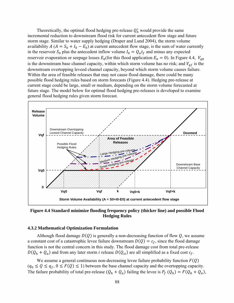
88

Theoretically, the optimal flood hedging pre-release ∗ would provide the same incremental reduction to downstream flood risk for current antecedent flow stage and future storm stage. Similar to water supply hedging (Draper and Lund 2004), the storm volume availability ( ) at current antecedent flow stage, is the sum of water currently in the reservoir plus the antecedent inflow volume and minus any expected reservoir evaporation or seepage losses (for this flood application 0). In Figure 4.4, is the downstream base channel capacity, within which storm volume has no risk; and is the downstream overtopping leveed channel capacity, beyond which storm volume causes failure. Within the area of feasible releases that may not cause flood damage, there could be many possible flood hedging rules based on storm forecasts (Figure 4.4). Hedging pre-release at current stage could be large, small or medium, depending on the storm volume forecasted at future stage. The model below for optimal flood hedging pre-releases is developed to examine general flood hedging rules given storm forecast.

Figure 4.4 Standard minimize flooding frequency policy (thicker line) and possible Flood Hedging Rules

4.3.2 Mathematical Optimization Formulation

Although flood damage is generally a non-decreasing function of flow , we assume a constant cost of a catastrophic levee failure downstream , since the flood damage function is not the central concern in this study. The flood damage cost from total pre-release

and from any later storm release are all simplified as a fixed cost .

We assume a general continuous non-decreasing levee failure probability function ( , 0 1) between the base channel capacity and the overtopping capacity. The failure probability of total pre-release failing the levee is ,

Storm Volume Availability (A = S0+I0-E0) at current antecedent flow stage

Release Volume

Vqf

Vqf+k

Downstream Overtopping Leveed Channel Capacity

Vq0

Doomed

Large Hedging pre-release

Vqf 0

Vq0+k Vq0

Medium Hedging pre-release

Small Hedging pre-release

k

Area of Feasible Releases

Downstream Base Channel Capacity

Possible Flood Hedging Rules

89

and the failure probability of storm release failing the levee is . Generally as two successive events, a future failure probability would be affected by the current event

. Here we assume the levee failure probabilities at two stages are independent. Flood risk in this two-stage model comes from current stage pre-release and future stage storm release, which are two not-mutually-exclusive independent events (Feller 2008). So for any possible storm , the probability it fails the downstream levee is pre-release failure probability plus the pre-release reliability (one minus the failure probability) multiplied by storm

release failure probability 1 . Summation of the failure probability over all possible storms is the overall failure probability of this flood event covering two stages.

This leads to the following mathematical optimization formulation, which minimizes the expected value of downstream flood damage summed over the pre-release and storm periods.

Min ∑ 1 (4.1.a)

Or

Min 1 ∑ (4.1.b)

Subject to:

, ∀ 1: (4.2)

(4.3)

, ∀ 1: (4.4)

0 (4.5)

where, is the probability of possible storm ; and are the failure probability of total pre-release and storm release; is the volume of storm stored in the reservoir; is the volume of storm , assumed to be a square hydrograph; is the release rate from the reservoir during storm ; is the duration of storm ’s reservoir inflows; is the reservoir’s total flood storage capacity; is the reservoir’s initial storage; is the pre-release hedging flow rate; is the flood forecast period in advance of the coming storm; is the antecedent inflow rate; is the downstream base channel capacity (with no levee failure) possibility; is the downstream over-topping channel capacity, with a failure probability of 1.

The first three constraints (Eqn. 4.2 to Eqn. 4.4) are some basic assumptions. Storage capacity constraint (upper bound of storage) that the reservoir cannot store more than its available capacity (Eqn. 4.2); release capacity constraint (upper bound of release/lower bound of storage) that pre-release volume cannot exceed the initial reservoir storage (Eqn. 4.3); and water balance constraint that all storm flood volumes must be stored or released during the storm, with no water losses (Eqn. 4.4). The last constraint (Eqn. 4.5) is non-negativity of the hedging pre-release flow rate , which is also a release capacity constraint (lower bound of release).

90

The two terms in the minimization objective (Eqn. 4.1.b) represent the expected downstream flood damage costs (flood risk) from current stage pre-release (

), and the expected downstream flood damage costs from future stage storm releases ( 1 ∑ ). The flood operation process includes a first stage of antecedent flow with pre-release and a second stage of flood flow. This two-stage decision formulation can be solved by a one-dimension search over the range of feasible hedging pre-release , with the other variables determined by the constraint equations.

This simple formulation illustrates many aspects of the problem. For more complex storms and storm forecasts, third or fourth stages of pre-releases and storm release decisions might be added, with a consequent increase in parameter estimation and computational effort.

4.3.3 Small, Intermediate and Large Storms

To distinguish the flood risks at future stages, we divided the forecasted storms into three groups, according to its likelihood triggering a levee failure (Figure 4.5). A linear failure probability curve is used in Figure 4.5 for initial illustration purposes.

(1) Small storms, where later storm releases pose no threat to the levee ( 0) even with no pre-release, but a flood pre-releases would increase current risk at a failure probability of . The occurrence probability of such small storms is the probability that hedging pre-

releases will be futile, increasing immediate risk without helping later flood protection.

(2) Intermediate storms, where pre-releases increase storage capacity to significantly decrease later storm releases, but later storm releases would still threaten the levee at a failure probability of (0 1). Overall flood risks exist in two stages with a failure probability 1 .

(3) Large storms, which would overwhelm the reservoir and levee regardless of pre-release decision, with a 1 levee failure probability for future stage and overall flood risk.

Volume and duration of forecasted storms would determine the categorization of the small, intermediate and large storms.

The flood volume boundary between small and intermediate storms is at oncoming flood volume , where 0 and . Besides the given reservoir and channel parameters, the number of small storms within this boundary depends on the characteristics of forecasted storm volume and duration . Of possible storms that are forecasted, the number of small storms is defined as , for which hedging pre-releases would raise risks of levee failure without reducing second-stage flood risks.

The system is completely overwhelmed (and doomed to fail) if flood volume exceeds available storage even with maximal pre-releases plus channel capacity, so the flood volume boundary between intermediate and large storms is . Meanwhile, , since pre-release volume cannot exceed initial storage. If pre-releases empty the entire initial storage, the boundary is . The number of storms not overwhelming the system is defined as of the total forecasted storms, depending on the characteristics of forecasted storm volume and duration . So the number of intermediate storms is , and there are large storms.

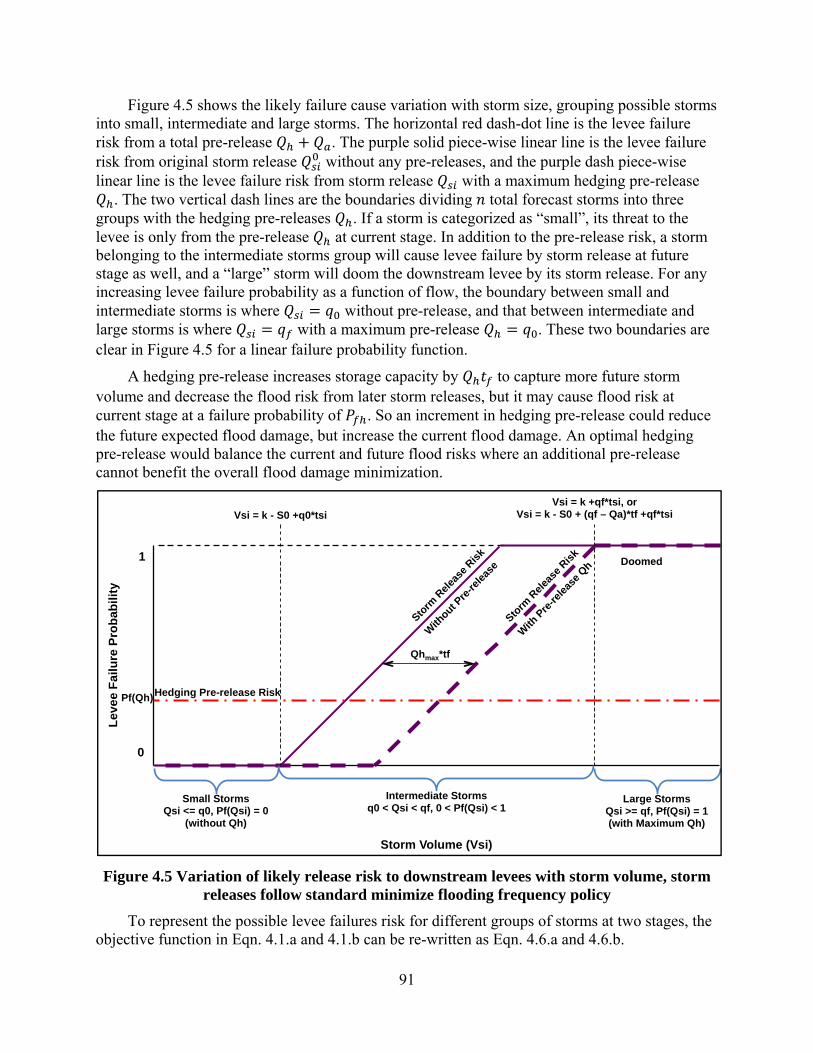
91

Figure 4.5 shows the likely failure cause variation with storm size, grouping possible storms into small, intermediate and large storms. The horizontal red dash-dot line is the levee failure risk from a total pre-release . The purple solid piece-wise linear line is the levee failure risk from original storm release without any pre-releases, and the purple dash piece-wise linear line is the levee failure risk from storm release with a maximum hedging pre-release

. The two vertical dash lines are the boundaries dividing total forecast storms into three groups with the hedging pre-releases . If a storm is categorized as “small”, its threat to the levee is only from the pre-release at current stage. In addition to the pre-release risk, a storm belonging to the intermediate storms group will cause levee failure by storm release at future stage as well, and a “large” storm will doom the downstream levee by its storm release. For any increasing levee failure probability as a function of flow, the boundary between small and intermediate storms is where without pre-release, and that between intermediate and large storms is where with a maximum pre-release . These two boundaries are clear in Figure 4.5 for a linear failure probability function.

A hedging pre-release increases storage capacity by to capture more future storm volume and decrease the flood risk from later storm releases, but it may cause flood risk at current stage at a failure probability of . So an increment in hedging pre-release could reduce the future expected flood damage, but increase the current flood damage. An optimal hedging pre-release would balance the current and future flood risks where an additional pre-release cannot benefit the overall flood damage minimization.

Figure 4.5 Variation of likely release risk to downstream levees with storm volume, storm releases follow standard minimize flooding frequency policy

To represent the possible levee failures risk for different groups of storms at two stages, the objective function in Eqn. 4.1.a and 4.1.b can be re-written as Eqn. 4.6.a and 4.6.b.

Small Storms Qsi <= q0, Pf(Qsi) = 0

(without Qh)

1

Storm

Rel

ease

Ris

k

With

out Pre

-rele

ase

Pf(Qh)

Intermediate Storms q0 < Qsi < qf, 0 < Pf(Qsi) < 1

Doomed

Large Storms Qsi >= qf, Pf(Qsi) = 1 (with Maximum Qh)

0

Lev

ee

Fa

ilu

re P

rob

abil

ity

Qhmax*tf

Storm

Rel

ease

Ris

k

With

Pre

-rele

ase

Qh

Hedging Pre-release Risk

Storm Volume (Vsi)

Vsi = k - S0 +q0*tsi Vsi = k +qf*tsi, or

Vsi = k - S0 + (qf – Qa)*tf +qf*tsi

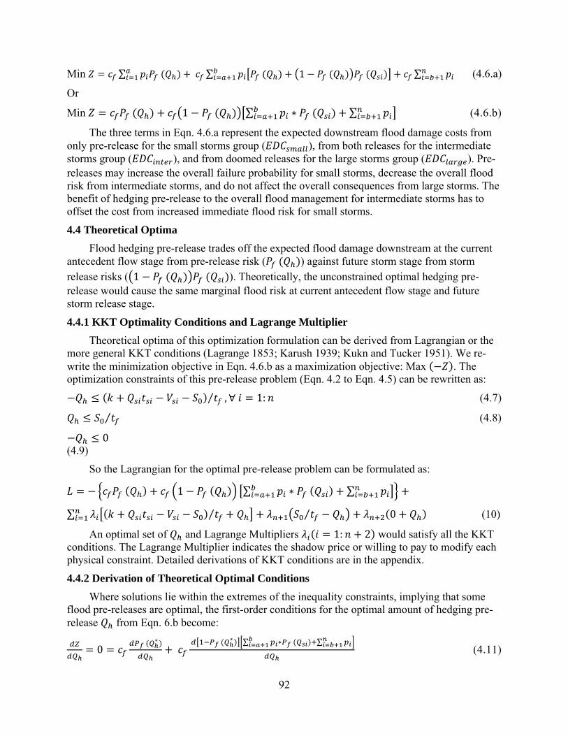
92

Min ∑ ∑ 1 ∑ (4.6.a)

Or

Min 1 ∑ ∗ ∑ (4.6.b)

The three terms in Eqn. 4.6.a represent the expected downstream flood damage costs from only pre-release for the small storms group ( ), from both releases for the intermediate storms group ( ), and from doomed releases for the large storms group ( ). Pre-releases may increase the overall failure probability for small storms, decrease the overall flood risk from intermediate storms, and do not affect the overall consequences from large storms. The benefit of hedging pre-release to the overall flood management for intermediate storms has to offset the cost from increased immediate flood risk for small storms.

4.4 Theoretical Optima

Flood hedging pre-release trades off the expected flood damage downstream at the current antecedent flow stage from pre-release risk ( ) against future storm stage from storm release risks ( 1 ). Theoretically, the unconstrained optimal hedging pre-release would cause the same marginal flood risk at current antecedent flow stage and future storm release stage.

4.4.1 KKT Optimality Conditions and Lagrange Multiplier

Theoretical optima of this optimization formulation can be derived from Lagrangian or the more general KKT conditions (Lagrange 1853; Karush 1939; Kukn and Tucker 1951). We re-write the minimization objective in Eqn. 4.6.b as a maximization objective: Max . The optimization constraints of this pre-release problem (Eqn. 4.2 to Eqn. 4.5) can be rewritten as:

⁄ , ∀ 1: (4.7)

⁄ (4.8)

0 (4.9)

So the Lagrangian for the optimal pre-release problem can be formulated as:

1 ∑ ∗ ∑

∑ ⁄ ⁄ 0 (10)

An optimal set of and Lagrange Multipliers 1: 2 would satisfy all the KKT conditions. The Lagrange Multiplier indicates the shadow price or willing to pay to modify each physical constraint. Detailed derivations of KKT conditions are in the appendix.

4.4.2 Derivation of Theoretical Optimal Conditions

Where solutions lie within the extremes of the inequality constraints, implying that some flood pre-releases are optimal, the first-order conditions for the optimal amount of hedging pre-release from Eqn. 6.b become:

0 ∗

∗ ∑ ∗ ∑

(4.11)

93

The current marginal downstream flood damage cost from pre-release is

, and the future marginal expected downstream flood damage cost from

storm releases is ∑ ∗ ∑

. So the

ideal theoretical optimal condition equalizes the two marginal expected damages that ∗ ∗ .

For this case with a constant potential damage cost, the levee failure cost does not affect the optimal hedging pre-release decision (Eqn. 4.11). So we can drop from the optimality condition:

∗ ∗

∑ ∗ ∑ 1 ∗ ∑

(4.12a)

1 is the current first stage non-failure probability or the reliability that pre-

release does not cause levee failure. If incorporating 0 and

0 for

“small” storms ( 1: ), and 1 and

0 for “large” storms ( 1: ),

the expected levee failure probability at future second stage from intermediate and large storms

is ∑ ∗ 0 ∑ ∗ ∑ ∗ 1 ∑ ∗ ,

and its derivative (the expected marginal future levee failure probability) is

∑ ∗ 0 ∑ ∗

∑ ∗ 0 ∑

. So we can have a

general optimal condition:

∗

1 ∗ ∗

1 ∗ ,

(4.12.b)

∗

∗

∗

∗ ,

(4.12.c)

∗ ∗

∗ ∗

(4.12.d)

The left hand side of Eqn. 4.12.b means the change in ∗ given no expected failure in the future stage, and the right hand side means the expected change in ∗ given no failure in the current stage. This optimality condition (Eqn. 4.12.b) implies equalizing the weighted marginal effectiveness at reducing failure in each stage. The ratio of non-failure (reliability)

probability ( ∗

∗ ) in Eqn. 4.12.c and 4.12.d evaluate the relative marginal effectiveness

at reducing failure in two stages.

By substituting ⁄ / (from the relation / ), we have the following optimal condition for hedging pre-releases:

94

∗

∗ ∑

∑

(4.12.e)

Eqn. 4.12.e implies that the optimal hedging pre-release ∗ is where ratio of the increment in pre-release failure probability divided by forecast period to the pre-release reliability, equals ratio of the expected increment in storm release failure probabilities each divided by its duration to the expected storm release reliability. The important role of forecast period and storm duration here is because of the assumed square hydrographs.

If any constraints bind on the optimal results, the theoretical optimal condition in Eqn. 4.12 may not be satisfied.

Implications of the theoretical optimal condition from Eqn. 4.12 are summarized below. (1) For a constant damage cost, the optimal flood hedging pre-release in this case occurs

when the current marginal downstream flood probability from pre-release equals the future marginal expected downstream flood probability from later storm releases. The amount of failure damage drops from the optimal solution.

(2) The optimal flood hedging pre-release depends on the frequencies of intermediate storms and originally harmless small storms, but not storms large enough to overwhelm the system (having a levee failure probability of one), since even hedging pre-release cannot change the fact that the system will fail. However, storm probabilities are correlated that sum to one.

(3) Having possible intermediate storms, which can be controlled only if pre-releases are made, is a necessary condition for flood hedging to be optimal. Flood hedging for small storms is not worthwhile as there is no storm release risk. And pre-releases are futile for large storms. So hedging pre-release would be large with more intermediate storms forecasted, while it would be small with fewer intermediate storms forecasted (Figure 4.4).

(4) Longer forecast periods can make flood hedging releases more desirable, as a unit of hedging pre-release volume ( ) will drive less increase in hedging release rate and levee failure probability. According to Eqn. 4.12.e, given fixed marginal failure probabilities from pre-release or storm releases for optimal pre-release, increasing forecast period decreases the ratio for the current stage, or increases the ratio for future stage. Therefore, optimal hedging pre-release would increase with larger forecast periods.

(5) Shorter oncoming storm durations make flood hedging pre-release more effective, as a given hedging pre-release volume will reduce peak outflows more to further reduce levee failure risk for a forecast storm.

The optimal hedging pre-release for a linear failure probability curve will be larger than that for a concave failure probability curve, and will be less for a convex failure probability curve. First, the failure probability of a concave curve is the highest for any given flow, that of a convex curve is the lowest, and that of a linear curve is in between (Figure 4.2). Second, a linear failure probability function has constant marginal values (0 second-order derivative), a concave failure probability curve has decreasing marginal increases (negative second-order derivative), and a convex failure probability curve with increasing marginal increases (positive second-order derivative) as flow increases. Hedging pre-releases also affect the boundaries of storms groups. So a more convex initial shape to levee failure probabilities should induce more flood pre-release.

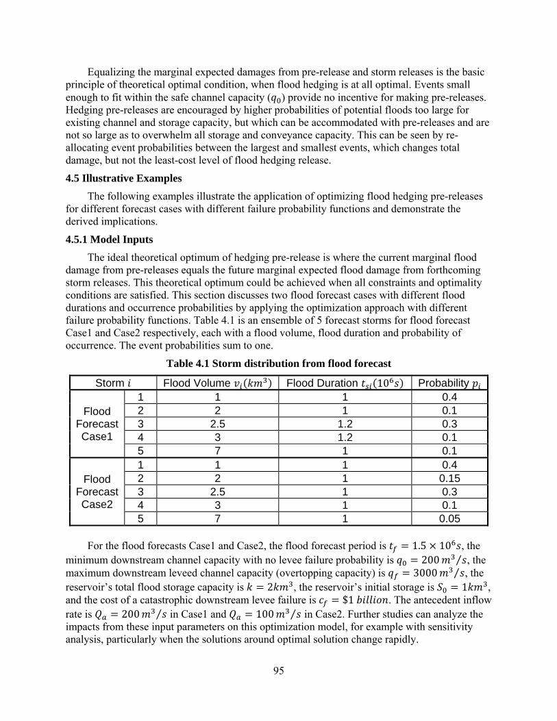
95

Equalizing the marginal expected damages from pre-release and storm releases is the basic principle of theoretical optimal condition, when flood hedging is at all optimal. Events small enough to fit within the safe channel capacity ( ) provide no incentive for making pre-releases. Hedging pre-releases are encouraged by higher probabilities of potential floods too large for existing channel and storage capacity, but which can be accommodated with pre-releases and are not so large as to overwhelm all storage and conveyance capacity. This can be seen by re-allocating event probabilities between the largest and smallest events, which changes total damage, but not the least-cost level of flood hedging release.

4.5 Illustrative Examples

The following examples illustrate the application of optimizing flood hedging pre-releases for different forecast cases with different failure probability functions and demonstrate the derived implications.

4.5.1 Model Inputs

The ideal theoretical optimum of hedging pre-release is where the current marginal flood damage from pre-releases equals the future marginal expected flood damage from forthcoming storm releases. This theoretical optimum could be achieved when all constraints and optimality conditions are satisfied. This section discusses two flood forecast cases with different flood durations and occurrence probabilities by applying the optimization approach with different failure probability functions. Table 4.1 is an ensemble of 5 forecast storms for flood forecast Case1 and Case2 respectively, each with a flood volume, flood duration and probability of occurrence. The event probabilities sum to one.

Table 4.1 Storm distribution from flood forecast

Storm Flood Volume Flood Duration 10 Probability

Flood Forecast Case1

1 1 1 0.4 2 2 1 0.1 3 2.5 1.2 0.3 4 3 1.2 0.1 5 7 1 0.1

Flood Forecast Case2

1 1 1 0.4 2 2 1 0.15 3 2.5 1 0.3 4 3 1 0.1 5 7 1 0.05

For the flood forecasts Case1 and Case2, the flood forecast period is 1.5 10 , the

minimum downstream channel capacity with no levee failure probability is 200 ⁄ , the maximum downstream leveed channel capacity (overtopping capacity) is 3000 ⁄ , the reservoir’s total flood storage capacity is 2 , the reservoir’s initial storage is 1 , and the cost of a catastrophic downstream levee failure is $1 . The antecedent inflow rate is 200 ⁄ in Case1 and 100 ⁄ in Case2. Further studies can analyze the impacts from these input parameters on this optimization model, for example with sensitivity analysis, particularly when the solutions around optimal solution change rapidly.

96

Constraining pre-release volume to less than the initial reservoir storage ( ) means the maximum pre-release is , 667 ⁄ . So the failure probabilities of pre-releases that exceed 667 ⁄ are infeasible.

According to the two boundaries for storms groups, in both cases, storm 1 is “small”, because it poses no threat to downstream even without pre-releases (failure probability from storm release is 0). Storm 5 will overwhelm the levee as a “large” storm. Storms 2, 3 and 4 are “intermediate” storms, since they still have failure probability with storm releases while may not yet be large enough to doom the levee.

Three typical levee failure probability functions are implemented in the optimization and compared: convex, linear and concave failure probability functions (Figure 4.2). Given two points, , 0 and , 1 , on the levee failure probability curve, we use three simple levee failure probability functions.

Quadratic Convex Function: 22

Linear Function:

Quadratic Concave Function: 2

21

A necessary condition for flood hedging pre-release to be optimal is the flood risk (expected overall damage) from flood release decisions within the feasible region is convex. Such convexity primarily depends on the failure probability function, and is also slightly affected by the probability distribution of forecast storms. So a convex failure probability function would clearly guarantee the convexity of the overall damage that hedging pre-release is desirable. The probability distribution of forecast storms dominates the optimal hedging pre-release with a linear failure probability function, and hedging pre-release would never be optimal with a concave failure probability function. These are shown in the examples below.

The optimizations below are solved by enumeration of expected failure damage costs over a range of hedging pre-releases in 1 ⁄ increment, with other variables determined by the constraints.

4.5.2 Results for Different Failure Probability Functions

Figure 4.6(a) and (b) are the optimization results with a convex failure probability function for Case1 and Case2 respectively. In Figure 4.6, the thickest blue solid lines read on the right vertical axis show the expected failure damage cost. Other lines on each figure are the varying levee failure probabilities of total pre-release and each storm release, and the varying expected overall failure probability with increasing hedging pre-release. The lines in Figure 4.7 and Figure 4.8 below have the same representations.

Generally, levee failure probability from the total pre-release increases with increasing hedging pre-release, leading to decreasing levee failure probability from the later storm release of each possible storm, except for the extreme small storms causing no failure and the extreme large storms which definitely fail the levee (Figure 4.6 and later Figure 4.7 and 4.8). “Small” storm 1 with a constant 0 failure probability and “large” storm 5 with a constant 1 failure probability for any pre-release decisions do not affect the optimal hedging pre-release.

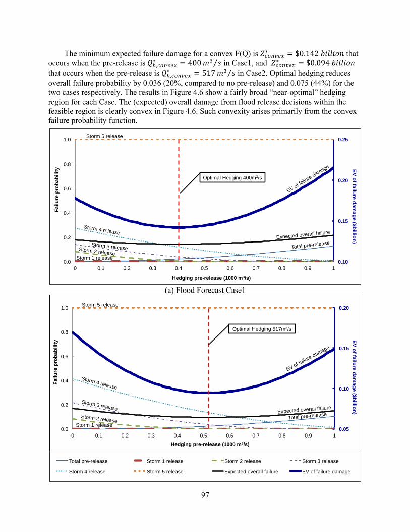
97

The minimum expected failure damage for a convex F(Q) is ∗ $0.142 that occurs when the pre-release is ,

∗ 400 ⁄ in Case1, and ∗ $0.094 that occurs when the pre-release is ,

∗ 517 ⁄ in Case2. Optimal hedging reduces overall failure probability by 0.036 (20%, compared to no pre-release) and 0.075 (44%) for the two cases respectively. The results in Figure 4.6 show a fairly broad “near-optimal” hedging region for each Case. The (expected) overall damage from flood release decisions within the feasible region is clearly convex in Figure 4.6. Such convexity arises primarily from the convex failure probability function.

(a) Flood Forecast Case1

0.10

0.15

0.20

0.25

0.0

0.2

0.4

0.6

0.8

1.0

0 0.1 0.2 0.3 0.4 0.5 0.6 0.7 0.8 0.9 1

Fai

lure

pro

bab

ilit

y

Hedging pre-release (1000 m3/s)

Optimal Hedging 400m3/s

EV

of failu

re dam

ag

e ($billio

n) Storm 3 release

Storm 4 release

Storm 5 release

Total pre-release Expected overall failure

EV of failure damage

Storm 2 release Storm 1 release

0.05

0.10

0.15

0.20

0.0

0.2

0.4

0.6

0.8

1.0

0 0.1 0.2 0.3 0.4 0.5 0.6 0.7 0.8 0.9 1

Fai

lure

pro

ba

bili

ty

Hedging pre-release (1000 m3/s)

Total pre-release Storm 1 release Storm 2 release Storm 3 release

Storm 4 release Storm 5 release Expected overall failure EV of failure damage

Storm 3 release

Storm 4 release

Storm 5 release

Total pre-release Expected overall failure

EV of failure damage

Storm 2 release Storm 1 release

Optimal Hedging 517m3/s

EV

of failu

re da

mag

e ($b

illion

)

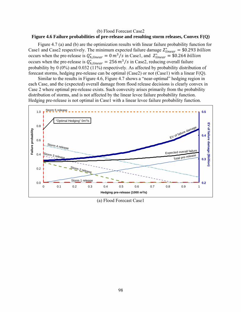
98

(b) Flood Forecast Case2 Figure 4.6 Failure probabilities of pre-release and resulting storm releases, Convex F(Q)

Figure 4.7 (a) and (b) are the optimization results with linear failure probability function for Case1 and Case2 respectively. The minimum expected failure damage ∗ $0.293 occurs when the pre-release is ,

∗ 0 ⁄ in Case1, and ∗ $0.264 occurs when the pre-release is ,

∗ 256 ⁄ in Case2, reducing overall failure probability by 0 (0%) and 0.032 (11%) respectively. As affected by probability distribution of forecast storms, hedging pre-release can be optimal (Case2) or not (Case1) with a linear F(Q).

Similar to the results in Figure 4.6, Figure 4.7 shows a “near-optimal” hedging region in each Case, and the (expected) overall damage from flood release decisions is clearly convex in Case 2 where optimal pre-release exists. Such convexity arises primarily from the probability distribution of storms, and is not affected by the linear levee failure probability function. Hedging pre-release is not optimal in Case1 with a linear levee failure probability function.

(a) Flood Forecast Case1

0.2

0.3

0.4

0.5

0.0

0.2

0.4

0.6

0.8

1.0

0 0.1 0.2 0.3 0.4 0.5 0.6 0.7 0.8 0.9 1

Fai

lure

pro

bab

ility

Hedging pre-release (1000 m3/s)

Storm 2 release

Storm 1 release

Storm 3 release

Storm 4 release

Storm 5 release

Total pre-release Expected overall failure

EV of failure damage

EV

of failu

re dam

age ($b

illion

)

“Optimal Hedging” 0m3/s

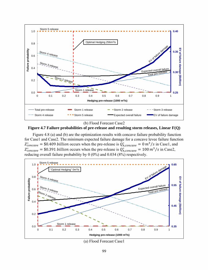
99

(b) Flood Forecast Case2

Figure 4.7 Failure probabilities of pre-release and resulting storm releases, Linear F(Q)

Figure 4.8 (a) and (b) are the optimization results with concave failure probability function for Case1 and Case2. The minimum expected failure damage for a concave levee failure function ∗ $0.409 occurs when the pre-release is ,

∗ 0 ⁄ in Case1, and ∗ $0.391 occurs when the pre-release is ,

∗ 100 ⁄ in Case2, reducing overall failure probability by 0 (0%) and 0.034 (8%) respectively.

(a) Flood Forecast Case1

0.25

0.30

0.35

0.40

0.0

0.2

0.4

0.6

0.8

1.0

0 0.1 0.2 0.3 0.4 0.5 0.6 0.7 0.8 0.9 1

Fai

lure

pro

bab

ility

Hedging pre-release (1000 m3/s)

Total pre-release Storm 1 release Storm 2 release Storm 3 release

Storm 4 release Storm 5 release Expected overall failure EV of failure damage

Storm 1 release

Storm 3 release

Storm 4 release

Storm 5 release

Total pre-release Expected overall failure

EV of fa

ilure

damag

e Optimal Hedging 256m3/s

Storm 2 release

EV

of failu

re dam

ag

e ($billio

n)

0.35

0.45

0.55

0.65

0.0

0.2

0.4

0.6

0.8

1.0

0 0.1 0.2 0.3 0.4 0.5 0.6 0.7 0.8 0.9 1

Fai

lure

pro

bab

ility

Hedging pre-release (1000 m3/s)

Storm 3 release

Storm 4 release

Total pre-release Expected overall failure

EV of failure damage

Storm 2 release

EV

of failu

re dam

ag

e ($billio

n)

Storm 1 release

Storm 5 release

“Optimal Hedging” 0m3/s

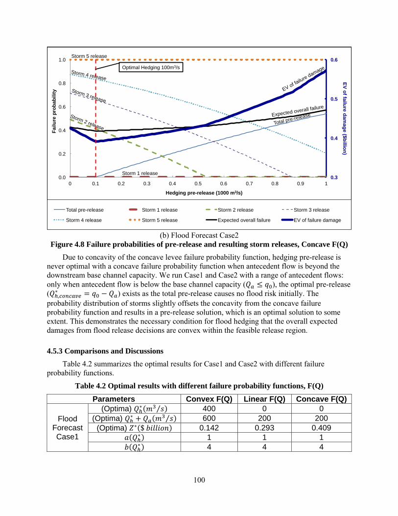
100

(b) Flood Forecast Case2

Figure 4.8 Failure probabilities of pre-release and resulting storm releases, Concave F(Q)

Due to concavity of the concave levee failure probability function, hedging pre-release is never optimal with a concave failure probability function when antecedent flow is beyond the downstream base channel capacity. We run Case1 and Case2 with a range of antecedent flows: only when antecedent flow is below the base channel capacity ( ), the optimal pre-release ( ,

∗ ) exists as the total pre-release causes no flood risk initially. The probability distribution of storms slightly offsets the concavity from the concave failure probability function and results in a pre-release solution, which is an optimal solution to some extent. This demonstrates the necessary condition for flood hedging that the overall expected damages from flood release decisions are convex within the feasible release region.

4.5.3 Comparisons and Discussions

Table 4.2 summarizes the optimal results for Case1 and Case2 with different failure probability functions.

Table 4.2 Optimal results with different failure probability functions, F(Q)

Parameters Convex F(Q) Linear F(Q) Concave F(Q)

Flood Forecast Case1

(Optima) ∗ ⁄ 400 0 0 (Optima) ∗ ⁄ 600 200 200

(Optima) ∗ $ 0.142 0.293 0.409 ∗ 1 1 1 ∗ 4 4 4

0.3

0.4

0.5

0.6

0.0

0.2

0.4

0.6

0.8

1.0

0 0.1 0.2 0.3 0.4 0.5 0.6 0.7 0.8 0.9 1

Fai

lure

pro

ba

bili

ty

Hedging pre-release (1000 m3/s)

Total pre-release Storm 1 release Storm 2 release Storm 3 release

Storm 4 release Storm 5 release Expected overall failure EV of failure damage

Storm 3 release

Storm 4 release

Storm 5 release

Total pre-release Expected overall failure

EV of failure damage

Storm 2 release

Storm 1 release

Optimal Hedging 100m3/s

EV

of failu

re dam

age ($b

illion

)

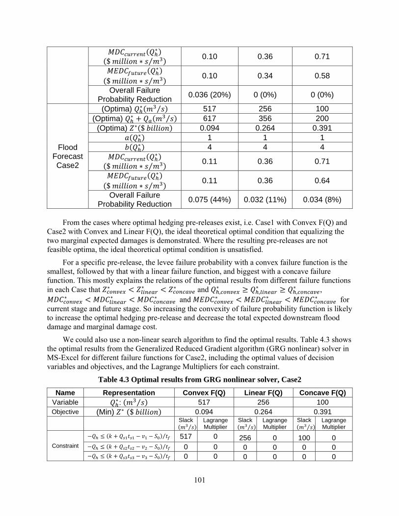
101

∗ $ ∗ ⁄

0.10 0.36 0.71

∗ $ ∗ ⁄

0.10 0.34 0.58

Overall Failure Probability Reduction

0.036 (20%) 0 (0%) 0 (0%)

Flood Forecast Case2

(Optima) ∗ ⁄ 517 256 100 (Optima) ∗ ⁄ 617 356 200

(Optima) ∗ $ 0.094 0.264 0.391 ∗ 1 1 1 ∗ 4 4 4

∗ $ ∗ ⁄

0.11 0.36 0.71

∗ $ ∗ ⁄

0.11 0.36 0.64

Overall Failure Probability Reduction

0.075 (44%) 0.032 (11%) 0.034 (8%)

From the cases where optimal hedging pre-releases exist, i.e. Case1 with Convex F(Q) and

Case2 with Convex and Linear F(Q), the ideal theoretical optimal condition that equalizing the two marginal expected damages is demonstrated. Where the resulting pre-releases are not feasible optima, the ideal theoretical optimal condition is unsatisfied.

For a specific pre-release, the levee failure probability with a convex failure function is the smallest, followed by that with a linear failure function, and biggest with a concave failure function. This mostly explains the relations of the optimal results from different failure functions in each Case that ∗ ∗ ∗ and ,

∗,∗

,∗ ,

∗ ∗ ∗ and ∗ ∗ ∗ for current stage and future stage. So increasing the convexity of failure probability function is likely to increase the optimal hedging pre-release and decrease the total expected downstream flood damage and marginal damage cost.

We could also use a non-linear search algorithm to find the optimal results. Table 4.3 shows the optimal results from the Generalized Reduced Gradient algorithm (GRG nonlinear) solver in MS-Excel for different failure functions for Case2, including the optimal values of decision variables and objectives, and the Lagrange Multipliers for each constraint.

Table 4.3 Optimal results from GRG nonlinear solver, Case2

Name Representation Convex F(Q) Linear F(Q) Concave F(Q) Variable ∗ : ⁄ 517 256 100 Objective (Min) ∗ $ 0.094 0.264 0.391

Slack

⁄Lagrange Multiplier

Slack⁄

Lagrange Multiplier

Slack⁄

Lagrange Multiplier

Constraint

⁄ 517 0 256 0 100 0 ⁄ 0 0 0 0 0 0 ⁄ 0 0 0 0 0 0

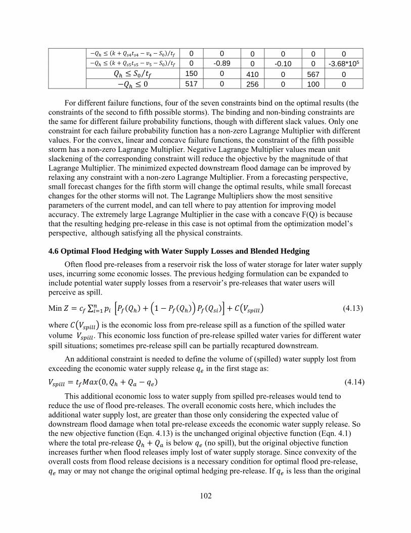
102

⁄ 0 0 0 0 0 0 ⁄ 0 -0.89 0 -0.10 0 -3.68*105

⁄ 150 0 410 0 567 0 0 517 0 256 0 100 0

For different failure functions, four of the seven constraints bind on the optimal results (the

constraints of the second to fifth possible storms). The binding and non-binding constraints are the same for different failure probability functions, though with different slack values. Only one constraint for each failure probability function has a non-zero Lagrange Multiplier with different values. For the convex, linear and concave failure functions, the constraint of the fifth possible storm has a non-zero Lagrange Multiplier. Negative Lagrange Multiplier values mean unit slackening of the corresponding constraint will reduce the objective by the magnitude of that Lagrange Multiplier. The minimized expected downstream flood damage can be improved by relaxing any constraint with a non-zero Lagrange Multiplier. From a forecasting perspective, small forecast changes for the fifth storm will change the optimal results, while small forecast changes for the other storms will not. The Lagrange Multipliers show the most sensitive parameters of the current model, and can tell where to pay attention for improving model accuracy. The extremely large Lagrange Multiplier in the case with a concave F(Q) is because that the resulting hedging pre-release in this case is not optimal from the optimization model’s perspective, although satisfying all the physical constraints.

4.6 Optimal Flood Hedging with Water Supply Losses and Blended Hedging

Often flood pre-releases from a reservoir risk the loss of water storage for later water supply uses, incurring some economic losses. The previous hedging formulation can be expanded to include potential water supply losses from a reservoir’s pre-releases that water users will perceive as spill.

Min ∑ 1 (4.13)

where is the economic loss from pre-release spill as a function of the spilled water volume . This economic loss function of pre-release spilled water varies for different water spill situations; sometimes pre-release spill can be partially recaptured downstream.

An additional constraint is needed to define the volume of (spilled) water supply lost from exceeding the economic water supply release in the first stage as:

0, (4.14)

This additional economic loss to water supply from spilled pre-releases would tend to reduce the use of flood pre-releases. The overall economic costs here, which includes the additional water supply lost, are greater than those only considering the expected value of downstream flood damage when total pre-release exceeds the economic water supply release. So the new objective function (Eqn. 4.13) is the unchanged original objective function (Eqn. 4.1) where the total pre-release is below (no spill), but the original objective function increases further when flood releases imply lost of water supply storage. Since convexity of the overall costs from flood release decisions is a necessary condition for optimal flood pre-release,

may or may not change the original optimal hedging pre-release. If is less than the original

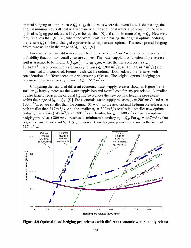
103

optimal hedging total pre-release ∗ that locates where the overall cost is decreasing, the original minimum overall cost will increase with the additional water supply lost. So the new optimal hedging pre-release is likely to be less than ∗ and at a minimum of . However, if is no less than ∗ where the overall cost is increasing, the original optimal hedging pre-release ∗ (in the unchanged objective function) remains optimal. The new optimal hedging pre-release will be in the range of [ , ∗].

For illustration, we add water supply lost to the previous Case2 with a convex levee failure probability function, so overall costs are convex. The water supply loss function of pre-release spill is assumed to be linear: , where the unit spill cost is $0.14/ . Three economic water supply releases (200 ⁄ , 400 ⁄ , 667 ⁄ ) are implemented and compared. Figure 4.9 shows the optimal flood hedging pre-releases with consideration of different economic water supply releases. The original optimal hedging pre-release without water supply losses is ∗ 517 ⁄ .

Comparing the results of different economic water supply releases shown in Figure 4.9, a smaller largely increases the water supply loss and overall cost for any pre-release. A smaller

also largely reduces the original ∗ and so reduces the new optimal hedging pre-release within the range of [ , ∗]. For economic water supply releases 200 ⁄ and 400 ⁄ , are smaller than the original ∗ , so the new optimal hedging pre-releases are both smaller than 517 ⁄ . And the smaller 200 ⁄ results in a smaller new optimal hedging pre-release (142 ⁄ 300 ⁄ ). Besides, for 400 ⁄ , the new optimal hedging pre-release 300 ⁄ reaches its minimum boundary . For 667 ⁄ that is greater than the original ∗ , the new optimal hedging pre-release remains the same at 517 ⁄ .

Figure 4.9 Optimal flood hedging pre-releases with different economic water supply release

0.0

0.1

0.2

0.3

0.4

0 0.1 0.2 0.3 0.4 0.5 0.6 0.7 0.8 0.9 1

Eco

no

mic

Co

sts

($b

illio

n)

Hedging pre-release (1000 m3/s)

Optimal Hedging 142m3/s,

qe=200m3/s

Optimal Hedging 300m3/s,

qe=400m3/s

Optimal Hedging 517m3/s,

no spill lost& qe=667m3/s

EV of failure damage, no water supply lost

EV of failure damage & qe=667m

3 /s

EV of failure damage & qe=400m

3 /s

EV of failure damage & qe=200m

3 /s

Wat

er s

uppl

y lo

st, q

e=40

0m3 /s

Wat

er s

uppl

y lo

st, q

e=20

0m3 /s

Wat

er s

uppl

y lo

st, q

e=66

7m3 /s

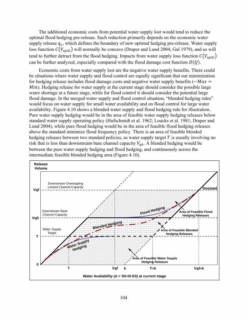
104

The additional economic costs from potential water supply lost would tend to reduce the optimal flood hedging pre-release. Such reduction primarily depends on the economic water supply release , which defines the boundary of new optimal hedging pre-release. Water supply loss function will normally be concave (Draper and Lund 2004; Gal 1979), and so will tend to further detract from the flood hedging. Impacts from water supply loss function can be further analyzed, especially compared with the flood damage cost function .

Economic costs from water supply lost are the negative water supply benefits. There could be situations where water supply and flood control are equally significant that our minimization for hedging release includes flood damage costs and negative water supply benefits (

). Hedging release for water supply at the current stage should consider the possible large water shortage at a future stage, while for flood control it should consider the potential large flood damage. In the merged water supply and flood control situation, “blended hedging rules” would focus on water supply for small water availability and on flood control for large water availability. Figure 4.10 shows a blended water supply and flood hedging rule for illustration. Pure water supply hedging would be in the area of feasible water supply hedging releases below standard water supply operating policy (Hufschmidt et al. 1962; Loucks et al. 1981; Draper and Lund 2004), while pure flood hedging would be in the area of feasible flood hedging releases above the standard minimize flood frequency policy. There is an area of feasible blended hedging releases between two standard policies, as water supply target is usually involving no risk that is less than downstream base channel capacity . A blended hedging would be between the pure water supply hedging and flood hedging, and continuously across the intermediate feasible blended hedging area (Figure 4.10).

Release Volume

Vqf

Vqf+k k

T

Water Availability (A = S0+I0-E0) at current stage

Doomed

Flood Hedging

T

Water Supply

Hedging

Vqf T+k 0

Area of Feasible Flood Hedging Releases

Vq0

Downstream Overtopping Leveed Channel Capacity

Downstream Base Channel Capacity

Water Supply Target

Area of Feasible Water Supply Hedging Releases

Area of Feasible Blended Hedging Releases

Blended Hedging

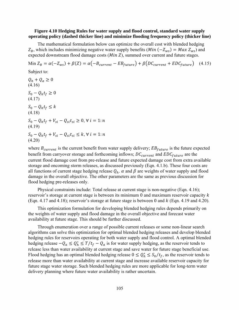
105

Figure 4.10 Hedging Rules for water supply and flood control, standard water supply operating policy (dashed thicker line) and minimize flooding frequency policy (thicker line)

The mathematical formulation below can optimize the overall cost with blended hedging , which includes minimizing negative water supply benefits ( ) and

expected downstream flood damage costs ( ), summed over current and future stages.

Min (4.15)

Subject to:

0 (4.16)

0 (4.17)

(4.18)

0, ∀ 1: (4.19)

, ∀ 1: (4.20)

where is the current benefit from water supply delivery; is the future expected benefit from carryover storage and forthcoming inflows; and are the current flood damage cost from pre-release and future expected damage cost from extra available storage and oncoming storm releases, as discussed previously (Eqn. 4.1.b). These four costs are all functions of current stage hedging release . and are weights of water supply and flood damage in the overall objective. The other parameters are the same as previous discussion for flood hedging pre-releases only.

Physical constraints include: Total release at current stage is non-negative (Eqn. 4.16); reservoir’s storage at current stage is between its minimum 0 and maximum reservoir capacity (Eqn. 4.17 and 4.18); reservoir’s storage at future stage is between 0 and (Eqn. 4.19 and 4.20).

This optimization formulation for developing blended hedging rules depends primarily on the weights of water supply and flood damage in the overall objective and forecast water availability at future stage. This should be further discussed.

Through enumeration over a range of possible current releases or some non-linear search algorithms can solve this optimization for optimal blended hedging releases and develop blended hedging rules for reservoirs operating for both water supply and flood control. A optimal blended hedging release ∗ ⁄ is for water supply hedging, as the reservoir tends to release less than water availability at current stage and save water for future stage beneficial use. Flood hedging has an optimal blended hedging release 0 ∗ ⁄ , as the reservoir tends to release more than water availability at current stage and increase available reservoir capacity for future stage water storage. Such blended hedging rules are more applicable for long-term water delivery planning where future water availability is rather uncertain.

106

4.7 Conclusions and Discussions

Flood hedging involves making water releases in advance of a coming flood event to make additional flood storage capacity available in the reservoir, as a way of reducing the probability of more severe flooding. Such pre-releases can involve the likely loss of water that would have value for water supply and might also involve pre-releases large enough to create small floods or small increases in downstream levee failures. Optimal flood hedging pre-release would minimize the overall expected damages to downstream areas. This paper develops an optimization approach for flood hedging pre-releases for a single reservoir, given an ensemble forecast of coming storms. Engineering uncertainty is incorporated considering levee overtopping and internal structural failures. According to the likely flood risk from pre-release and storm release, forecasted storms are divided into small, intermediate and large storms. Theoretical conditions for optimal flood hedging are then derived that equalize the marginal damages from current pre-release and the marginal expected damages from future storm releases. Large overwhelming storms do not affect the optimality of flood hedging pre-releases. The theoretical optima and its implications are derived and demonstrated. Additional economic costs from lost water supply storage could reduce the optimal flood hedging pre-release.

A convex overall expected failure damage from flood releases is a necessary condition for optimal flood hedging, which is primarily affected by the downstream levee failure probability function, the probability distribution of storm sizes, and the flood damage function. Flood hedging releases can only be optimal if flood or water supply losses from near-term releases are disproportionately smaller than consequent loss reductions from intermediate, but not overwhelming floods; this is a necessary, but not sufficient condition. There also must be a sufficiently high probability of large inflows requiring additional flood storage capacity created by pre-releases to prevent major flood damage (large, but not overwhelmingly large storms).

In some situations, flood reservoir operations should include hedging pre-releases, where reservoir releases are increased beyond the base channel capacity to reduce the overall likelihood of still higher flood releases from later storms. These flood hedging operations have some similarities with the water supply hedging operations in trading off between present and future benefits and risks.

In actual flood reservoir operations, there is often a reluctance to make large pre-releases that impose downstream damage as a way of reducing overall flood risk. This reluctance can be political in terms of those certain to be flooded downstream versus the praise from those who might be saved because of such pre-releases. This raises some institutional difficulties in terms of the ability of operators to follow more optimal risk-based operations.

4.8 References

Connaughton, J., King, N., Dong, L., Ji, P., & Lund, J. (2014). Comparing Simple Flood Reservoir Operation Rules. Water, 6(9), 2717-2731.

Draper, A. J., & Lund, J. R. (2004). Optimal hedging and carryover storage value. Journal of Water Resources Planning and Management, 130(1), 83-87.

Feller, W. (2008). An introduction to probability theory and its applications (Vol. 2). John Wiley & Sons.

Gal, S. (1979). Optimal management of a multireservoir water supply system. Water Resources Research, 15(4), 737-749.

107

Hufschmidt, M. M., Dorfman, R., Thomas Jr, H. A., Marglin, S. A., & Fair, G. M. (1962). Design of water-resource systems (pp. 443-458). Cambridge, MA: Harvard University Press.

Ji, P. (2011). Reservoir Re-operation, Risk, and Levee Failure Analysis: Mokelumne River Case (Vol. 72, No. 08), PhD dissertation, Department of Civil and Environmental Engineering, University of California – Davis

Karush, W. (1939). “Minima of Functions of Several Variables with Inequalities as Side Conditions,” M.S. thesis, Department of Mathematics, University of Chicago.

Kukn, H. W., & Tucker, A. W. (1951). Nonlinear programming. In Proceedings of second Berkeley symposium on mathematical statistics and probability (pp. 481-492).

Labadie, J. W. (2004). Optimal operation of multireservoir systems: State-of-the-art review. Journal of water resources planning and management, 130(2), 93-111.

Lagrange, J. L. (1853). Mécanique analytique (Vol. 1). Mallet-Bachelier. Loucks, D. P., Stedinger, J. R., & Haith, D. A. (1981). Water Resource Systems Planning and

Analysis. Prentice-Hall.. Lund, J. R. (2002). Floodplain planning with risk-based optimization. Journal of water resources

planning and management, 128(3), 202-207. Perlea, M., & Ketchum, E. (2011). Impact of Non-Analytical Factors in Geotechnical Risk

Assessment of Levees. Reston, VA: ASCE copyright Proceedings of Georisk 2011, June 26. 28, 2011, Atlanta, Georgia| d 20110000.

Shiau, J. T. (2011). Analytical optimal hedging with explicit incorporation of reservoir release and carryover storage targets. Water Resources Research, 47(1).

Stedinger, J. R. (1997). Expected probability and annual damage estimators. Journal of Water Resources Planning and Management, 123(2), 125-135.

USACE (2011), Cranford Levee reliability project for flood risk management Rahway, Cranford, NJ.

Wolff, T. F. (1997). Geotechnical reliability of levees. In Proc of a Hydrology and Hydraulics Workshop on Risk-Based Analysis for Flood Damage Reduction Studies, USACE, Hydrologic Engineering Center.

Wurbs, R. A. (1993). Reservoir-system simulation and optimization models. Journal of water resources planning and management, 119(4), 455-472.

You, J. Y., & Cai, X. (2008a). Hedging rule for reservoir operations: 1. A theoretical analysis. Water resources research, 44(1).

You, J. Y., & Cai, X. (2008b). Hedging rule for reservoir operations: 2. A numerical model. Water resources research, 44(1).

Zhao, J., Cai, X., & Wang, Z. (2011). Optimality conditions for a two‐stage reservoir operation problem. Water Resources Research, 47(8).

Zhao, T., Zhao, J., Lund, J. R., & Yang, D. (2014). Optimal Hedging Rules for Reservoir Flood Operation from Forecast Uncertainties. Journal of Water Resources Planning and Management.

4.9 Appendix

KKT Conditions

108

For the minimization formula in Eqn. 4.6 and the constraints in Eqn. 4.7 to Eqn. 4.9, we derived the Lagrangian in Eqn. 4.10. The KKT conditions for this optimal pre-release problem are below.

1. Gradient condition

0

∑ ∗ ∑∑ ⁄ ⁄ (A.1)

2. Feasibility conditions (optimization constraints)

⁄ , ∀ 1: (A.2) ⁄ (A.3) 0 (A.4)

3. Complementary slackness

⁄ 0, ∀ 1: (A.5) ⁄ 0 (A.6)

0 0 (A.7) 4. Non-negativity 0, for 1: 2 (A.8) 0 (A.9)

An optimal set of and 1: 2 would satisfy all these KKT conditions. The

Lagrange Multiplier ( is the right hand side of each constraint, 1: 2) is the

change in the minimized objective function if constraint is changed. is also named shadow price or dual variable which can tell the shadow value or willingness to pay for each physical constraint.

109

Conclusions There is a need for optimal design of levee and flood control systems with reservoir

operations, as significant components of the broad flood management portfolio. A variety of preparatory, response and recovery actions, and protection and vulnerability reduction actions within each category, should be implemented properly. Optimal designs of each individual action and their integration can provide economic benefits to the entire flood management system. This research developed new optimization design methods for individual flood management options, primarily with economically Risk-based analysis and Benefit-cost analysis and with physically technical designs.

Key contributions of this work include developing optimization models for designing new or evaluating existing single levees and simple levee systems with the well-known overtopping failure and the more frequent intermediate geotechnical failure, strategically analyzing the best levee system designs with different types of games and the way to achieve a system-wide economically optimal solution and to prevent inefficient outcomes, and developing hedging rules for optimal flood hedging pre-releases of a single reservoir to protect future possible large storms by creating a current small storm.

Since many assumptions and simplifications were made in this research, future studies should address these limitations in each individual work to help develop more optimal integrated flood management.

1. Potential damage cost in the entire work is assumed constant and to occur when a levee fails. Normally, damage cost should be a non-decreasing function of river flow or water level within the leveed channel. A wider range of flood damage cost functions should be used in future studies.

2. Channel geometry, hydrograph routing along a river channel, levee fragility curves and levee failure modes would affect single levee and simple levee system designs that would be benefit from more general representations. As longer levees should be more likely to fail, future work on optimal designs of levee(s) should include the effect of levee length.

3. Levee failure probability changes over time as a levee’s internal structure and external conditions evolve. So future study can analyze the dynamic evolution of the levee system design game, particularly changes of the resulting equilibriums and the Pareto-optimal outcomes.

4. Game theory can be applied to conflicting complex levee systems that involve multiple players to predict the different behaviors of each individual player and their coalitions, for example a multi-reach levee system with conflict between upstream and downstream land owners, and a ring levee system that each player is in charge of one levee section.

5. Blended hedging releases considering both hedging for water supply and for flood control could be developed for long term water release planning. The basic principle for optimal blended hedging releases should be balancing the current overall benefit/cost and the future overall benefit/cost.

6. Flood hedging pre-releases for a system with multiple correlated reservoirs, in series and/or in parallel, could be developed. Such hedging pre-releases involve the

110

economically beneficial trade-off among different reservoirs and that between current and future stages.

The optimally designed levee and flood control systems, which in this study have been developed with case studies in California, can be applied widely elsewhere. The Risk-based analysis and Benefit-cost analysis developed here for levee and flood control system design should, in principle, be extensible to designs of other individual flood management actions, which can be contrasted with the actions to manage other types of natural hazards, such as droughts and earthquakes. More importantly, these developed individual flood management actions can help design integrated flood management systems, which may require each action being optimally designed as part of an optimized portfolio of actions, meanwhile considering environmental and other water supply objectives for a broader range of beneficiaries.