Optimal Cost-Sharing in General Resource Selection Gamestheory.stanford.edu/~tim/papers/optcs.pdf · Gkatzelis, Kollias, and Roughgarden: Optimal Cost-Sharing in General Resource

Submitted to Operations Research

manuscript (Please, provide the manuscript number!)

Optimal Cost-Sharing in General Resource SelectionGames

Vasilis GkatzelisDepartment of Computer Science, Stanford University, Stanford, CA 94305, [email protected]

Konstantinos KolliasDepartment of Management Science and Engineering, Stanford University, Stanford, CA 94305, [email protected]

Tim RoughgardenDepartment of Computer Science, Stanford University, Stanford, CA 94305, [email protected]

Resource selection games provide a model for a diverse collection of applications where a set of resources is

matched to a set of demands. Examples include routing in traffic and in telecommunication networks, service

of requests on multiple parallel queues, acquisition of services or goods with demand-dependent prices, etc.

In reality, demands are often submitted by selfish entities (players) and congestion on the resources results in

negative externalities for their users. We consider a policy maker that can set a priori rules to minimize the

inefficiency induced by selfish players. For example, these rules may assume the form of scheduling policies

or pricing decisions. We explore the space of such rules abstracted as cost-sharing methods. We prescribe

desirable properties that the cost-sharing method should possess and prove that, in this natural design space,

the cost-sharing method induced by the Shapley value minimizes the worst-case inefficiency of equilibria.

Key words : resource selection, cost-sharing, Shapley value, price of anarchy, network routing

History : This paper was first submitted in October 2014.

1. Introduction

Resource selection games offer an abstraction for many interesting applications sharing a common

theme: there is a set of selfish demands (players) that choose a set of resources to use. The presence

of multiple players on the same resource causes an undesirable congestion effect which increases the

cost each one of them suffers. The applications that lie within this framework are diverse: routing

information packets in a telecommunications network or vehicles in a road network (Roughgarden

and Tardos (2002), Awerbuch et al. (2005)), constructing the infrastructure of a network (Anshele-

vich et al. (2008), Chen et al. (2010), von Falkenhausen and Harks (2013)), scheduling tasks for

1

Gkatzelis, Kollias, and Roughgarden: Optimal Cost-Sharing in General Resource Selection Games

2 Article submitted to Operations Research; manuscript no. (Please, provide the manuscript number!)

processing on parallel servers (Haviv and Roughgarden (2007)), and pricing congestion-dependent

services (Cominetti et al. (2009)). A common characteristic of these applications is that the joint

cost of a resource depends only on the total demand on that resource. Resource selection games

can be considered as generalizations of congestion games (Rosenthal (1973a)).

Enforcing a socially optimal allocation of the various resources (links, channels, roads, processors,

etc.) to the players is typically not feasible. We consider players that are not subject to centralized

control and pick the resources that allow them to optimize their own objectives. In the presence

of self-interested players, the obvious goal of a policy maker or system designer is to carefully

design the rules of the system to incentivize players to reach a socially desirable outcome. More

concretely, we assume that players reach an equilibrium of the induced game – a state such that

no unilateral deviation is beneficial to a player – and the goal is to provide a guarantee on how

well this equilibrium approximates a socially optimal allocation.

The way a policy maker or system designer can influence the game may vary, depending on the

application specifics, but a general abstraction that captures many such game-theoretic control

concepts is that of cost-sharing methods. In resource selection games the total demand that is

allocated to a specific resource generates a joint cost. This cost can be monetary (e.g., a total

payment requested for specific services) or not (e.g., aggregate queueing delay). The decision of

the policy maker then reduces to picking the cost-sharing method that determines which fraction

of this generated cost each of the users is responsible for.

Example: Routing of Packets in a Telecommunications Network. Consider the application of

routing packets from many different senders in a network. In typical cases, such as the Internet and

wireless networks, data from a sender to a receiver is sent on a fixed route. All packets that traverse

a given link in the network are initially queued and then forwarded by the local router. Each

sender has a given rate of injecting packets in the network and selects the route that minimizes

the total delay of her packets over all links (queues) they traverse. Consider a given link in the

network and the corresponding queue, which for the sake of this example can be assumed to be


Article submitted to Operations Research; manuscript no. (Please, provide the manuscript number!) 3

M/M/1. The arrival rate at the queue is given by the sum of rates of the users of the link (i.e., all

senders that include this link in their routes). This total arrival rate can be used to calculate the

M/M/1 average delay of a packet on this link. The total delay is then given as the product of the

average delay and the number of packets. A cost-sharing method in this setting would correspond

to a scheduling policy that assigns priorities to different senders. Rearranging the order of packets

in the queue, without introducing any idle time, does not impact the average delay and, hence,

each policy yields a different method of sharing the same joint cost (Shenker (1995), Mosk-Aoyama

and Roughgarden (2009)). We note that the converse does not hold and that in this application

not every cost-sharing method can be implemented by a scheduling policy (see Coffman Jr. and

Mitrani (1980) for a characterization).

Example: Economics of the Transportation of Goods. In the spirit of Cominetti et al. (2009),

consider the transportation of goods by logistics and freight companies. Shipments go through

transportation hubs such as airports, harbors, and train stations where operational costs vary

depending on the total volume of shipments. Freight companies are then charged fees which cover

these operational costs. The objective of each freight company is to identify the least costly route

between the origin and destination of their shipment. In such situations where the joint cost is mon-

etary, the connection with cost-sharing methods is clear and unrestricted. The policy maker designs

the method that distributes the operational costs to the companies using each transportation hub.

We assume that the policy maker seeks the cost-sharing method that maximizes the efficiency

of the resulting outcome. The design space is vast and we next identify some important properties

that the cost-sharing method should possess (Chen et al. (2010), von Falkenhausen and Harks

(2013)) and that give a crisper image of the available alternatives. We give an informal definition

of these properties here and present them formally in Section 2.

1. Budget-balance: the joint cost on each resource is covered precisely by its users.

2. Stability : the induced resource selection game is guaranteed to possess an equilibrium.

3. Locality : cost-sharing on a resource is independent of the system’s state beyond that resource.



Property 1 requests that the cost shares exactly cover the joint cost. We also consider the

impact of overcharging the players in Section 5. Property 2 requires that the cost-sharing method

guarantees the existence of a pure Nash equilibrium, which is crucial in many applications. Again,

we discuss the case of dropping this condition in our conclusions. Finally, Property 3 is important

for resource selection games since all the motivating applications concern large systems where

knowledge regarding the state of the system beyond the resource at hand is either infeasible or

very costly. Also, in such systems, resources are added and removed constantly so introducing

complicated dependencies among them is bound to cause scalability issues to the system. We call

a cost-sharing method admissible if it possesses all three properties.

1.1. Our Contributions and Paper Structure

We study resource selection games from the policy maker’s perspective and, given any set of

allowable convex and increasing joint resource cost functions, we characterize the optimal admissible

cost-sharing method. Our main result states that, among all such methods, the (unweighted)

Shapley value (Shapley (1953)) is the one that minimizes the worst-case price of anarchy, i.e., the

worst-case ratio between the total player cost in an equilibrium to the total player cost in the

socially optimal allocation of demands to resources.

In Section 2 we present our model and some examples. To illustrate our main ideas, we present

a case study on resource selection games with polynomial cost functions in Section 3. There, we

examine the performance of a class of parameterized Shapley values such that a single parameter

controls the relative advantage or disadvantage that is given to players with larger demand. We

characterize the price of anarchy as a function of this parameter and we prove that it is minimized

when the parameter is zero (which corresponds to the Shapley value). In Section 4 we strengthen

this result by showing that the Shapley value remains optimal among all admissible cost-sharing

methods for all convex cost functions. We conclude our paper and discuss extensions to cost-

sharing methods that are not admissible in Section 5. Omitted proofs are included in the electronic

companion section of the paper.



1.2. Related Work

The performance of cost-sharing methods in resource selection games has recently received a lot

of attention, leading to a sequence of results including the work of Chen et al. (2010) and von

Falkenhausen and Harks (2013), which is the most relevant to our results. In Chen et al. (2010),

the authors examine the whole space of admissible cost-sharing methods as well, but in networks

where all players have equal demand and the cost functions of the resources are constant, i.e., in a

setting with positive externalities. Their results exhibit optimality of the Shapley value in directed

networks and optimality of (non-Shapley) simple priority protocols for undirected networks. The

work of von Falkenhausen and Harks (2013) studies the inefficiency of cost-sharing methods in a

model very similar to the one we adopt here. The differences from our approach are the following:

first, rather than considering arbitrary strategy sets like we do, von Falkenhausen and Harks (2013)

focus on games where the players’ strategies are singletons or matroids. Also, von Falkenhausen

and Harks (2013) keep the set of allowable cost-functions unrestricted and prove that the price of

anarchy of any admissible cost-sharing method is unbounded. Apart from admissible cost-sharing

methods they also consider methods that violate the locality property in different ways and they

characterize the optimal method in each case.

Cost-sharing methods for resource selection games were also the focus of Harks and Miller (2011),

Marden and Wierman (2013), and Gopalakrishnan et al. (2013). In Harks and Miller (2011), the

authors study the performance of several cost-sharing methods in a slightly modified setting, where

each player declares a different demand for each resource. Marden and Wierman (2013) study

various cost-sharing methods in a utility maximization model for the players, while Gopalakrishnan

et al. (2013) characterized the space of admissible cost-sharing methods as the set of generalized

weighted Shapley values; a characterization that we will use in this work.

An interesting family of resource selection games is the class of weighted congestion games.

There has been a long line of work on these games focusing on the proportional sharing method,

according to which the players share their joint cost in proportion to the size of their demands



(Rosenthal (1973b), Milchtaich (1996), Monderer and Shapley (1996), Awerbuch et al. (2005),

Gairing and Schoppmann (2007), Bhawalkar et al. (2010), Harks and Klimm (2012), Harks et al.

(2011)). Proportional sharing is not an admissible cost-sharing method because it does not always

guarantee the existence of an equilibrium, except for special cases such as when the per unit of load

cost functions are quadratic or exponential (Fotakis and Spirakis (2008), Harks and Klimm (2012)).

Kollias and Roughgarden (2011) were the first to propose using Shapley value based methods in

congestion games in order to restore stability.

The impact of cost-sharing methods on the quality of equilibria has also been studied in other

models: Moulin and Shenker (2001) focused on participation games, while Moulin (2008) and

Mosk-Aoyama and Roughgarden (2009) studied queueing games. Also, very closely related in spirit

is previous work on coordination mechanisms, beginning with Christodoulou et al. (2009) and

subsequently in Immorlica et al. (2009), Azar et al. (2008), Caragiannis (2009), Abed and Huang

(2012), Kollias (2013), Cole et al. (2013), Christodoulou et al. (2014), and Bhattacharya et al.

(2014). Most work on coordination mechanisms concerns scheduling games and how the price of

anarchy varies with the choice of local machine policies (i.e., the order in which to process jobs

assigned to the same machine). Some of the recent work comparing the price of anarchy of different

auction formats, such as Lucier and Borodin (2010), Bhawalkar and Roughgarden (2012), and

Syrgkanis and Tardos (2013) also has a similar flavor.

2. The Model

In this section, we provide more details regarding our model. We begin with a set of definitions

(Section 2.1) and then we expand on how this model applies to our motivating applications.

2.1. Definitions

Definition 1 (Resource selection game). A resource selection game is defined by a tuple

(N,R,A,w,C,Ξ). N is a finite set of players, R is a finite set of resources, and A=×i∈NAi is the

set of strategy profiles, with Ai ⊆ 2R being the strategy set of player i. The vector w = (wi)i∈N

contains the demand wi of each player i, and C = (Cr)r∈R is a vector with Cr : R≥0 → R≥0 being

the cost function of resource r. Finally, Ξ is a cost-sharing method (defined below).



We write l(S) =∑

i∈S wi to denote the total demand of the players in S ⊆N . Given a strategy

vector A ∈ A, we write Sr(A) = {i ∈ N : r ∈ Ai} for the set of users of resource r. For ease of

notation we also use lr(A) for l(Sr(A)), the total demand on resource r. Function Cr outputs the

joint cost on the corresponding resource r as Cr(lr(A)).

Example 1. Consider a game with two players N = {1,2} having demands w1 =w2 = 1, and two

resources R = {a, b} with cost functions Ca(x) = x2 and Cb(x) = 2 · x3. The action sets are A1 =

A2 = {{a},{b}}, which means that each of the players will use exactly one of the resources. If A1 =

A2 = {a} (both players decide to use resource a), then the total demand on a is la(A) = 2 and the

joint cost on a is Ca(la(A)) = Ca(2) = 4. Now, if A1 =A2 = {b} (both players use resource b) and

the total demand on b is lb(A) = 2 leading to a joint cost of Cb(lb(A)) =Cb(2) = 16. Finally, if the

players decide to use different resources, then Ca(la(A)) =C(1) = 1 and Cb(lb(A)) =Cb(1) = 2.

A cost-sharing method Ξ defines a cost share function ξi,r :A→R≥0 for all i∈N and r ∈R. The

total cost of a player i, when the strategy profile is A, is ξi(A) =∑

r∈Aiξi,r(A). We proceed with

the definition of a pure Nash equilibrium.

Definition 2 (pure Nash equilibrium). The strategy vector A is a pure Nash equilibrium

(PNE) if for every player i and every A′i ∈Ai

ξi(A) ≤ ξi(A′i,A−i). (1)

Example 2. We revisit the game from Example 1 and suppose the cost-sharing method simply

dictates that the users of each resource share the joint cost of that resource equally. For example,

consider the A1 = A2 = {a} case. The joint cost is 4 and hence for both players we get ξ1(A) =

ξ2(A) = 2. If any of them were to deviate to strategy {b}, the incurred cost would be Cb(1) = 2,

which shows that the equilibrium condition (1) holds. The same can be shown for the outcome A1 =

{a} and A2 = {b}. Player 1 has cost ξ1(A) = 1 while, by deviating to the outcome A′ = ({b},{b}),

she would have a cost ξ1(A′) = Cb(2)/2 = 8. Similarly Player 2 suffers cost ξ2(A) = 2, while by

deviating to outcome A′′ = ({a},{a}), she would incur a cost ξ2(A′′) =Ca(2)/2 = 2. Note that the



PNE ({a},{a}) has total cost 4, while the PNE ({a},{b}) has total cost 2 (which is also the optimal

total cost).

We now formally define the properties that make cost-sharing method Ξ admissible.

Definition 3 (Cost-sharing method properties). An admissible method Ξ satisfies:

1. Budget-balance: for every resource r, Cr(A) =∑

i∈Sr(A) ξi,r(A), and ξi,r(A) = 0 if i /∈ Sr(A).

2. Stability : every induced game (N,R,A,w,C,Ξ) always possesses at least one PNE.

3. Locality : for every r ∈R and any two profiles A,A′ ∈A with Sr(A) = Sr(A′), ξi,r(A) = ξi,r(A

′)

The work of Gopalakrishnan et al. (2013) shows that the set of methods satisfying the above

properties are precisely the weighted variants of the Shapley value, which we define next.

Definition 4 (Shapley value). Consider a resource r and the set Sr(A) of its users. For a given

ordering π of the players in Sr(A), let Sπ,ir (A) denote the players preceding i in π. Then, the

quantity Cr(l(Sπ,ir (A)) +wi)−Cr(l(S

π,ir (A))) is the marginal increase in the joint cost caused by

player i when only the players preceding her in π and herself are using the resource. The Shapley

value of a Player i ∈ Sr(A) is the expected value of this increase with respect to the uniform

distribution over all orderings π:

ξSVi,r (A) = Eπ∼uniform

[

Cr(l(Sπ,ir (A))+wi)−Cr(l(S

π,ir (A)))

]

. (2)

Weighted variants of the Shapley value use non-uniform distributions over orderings. To be more

precise, these variants assign a positive sampling weight λi to each player i and they iteratively

pick the player that goes last in the ordering among the still unassigned players in each iteration,

with probabilities proportional to these sampling weights.

Definition 5 (Weighted Shapley value). A weighted Shapley value is defined by a vector λ

of sampling weights, one for each player. Given a resource r and its users Sr(A), consider the

following process of generating an ordering π of the players in Sr(A). The player that goes last

in the ordering is picked with probabilities proportional to the sampling weights, i.e., player i has



probability λi/∑

j∈Sr(A) λj of being the last player. The process is repeated with the penultimate

player being selected among the remaining ones in the same fashion, and so on. The weighted

Shapley value of player i is the expected increase she causes to the joint cost with respect to the

distribution ∆λ on orderings induced by λ:

ξwi,r = Eπ∼∆λ

[

Cr(l(Sπ,ir (A))+wi)−Cr(l(S

π,ir (A)))

]

. (3)

A weighted Shapley value with all sampling weights equal is equivalent to the Shapley value.

An important observation is that changing the cost-sharing method being used leads to a different

game, and hence to different equilibrium outcomes in the induced game. As a result, the efficiency

of this game crucially depends on the choice of the cost-sharing method. As a measure of the

inefficiency of an outcome A, we will be using the total cost Q(A) =∑

r∈RCr(lr(A)). In order to

quantify the quality of different cost-sharing methods we use the price of anarchy metric.

Definition 6 (Price of anarchy). Given a collection of cost functions C and a cost-sharing

method Ξ, the price of anarchy PoA(C,Ξ) is the worst-case ratio of equilibrium cost to optimal

cost over all resource selection games G = (N,R,A,w,C,Ξ) with Cr ∈ C for all r ∈R:

PoA(C,Ξ)= supG

maxA∈PNE(G)Q(A)

minA∗∈AQ(A∗). (4)

Recall, from Section 1, that meaningful PoA bounds are possible only if we parameterize these

bounds by the set of allowable resource cost functions. Hence, we assume that all resource cost

functions of the game come from a given set C, and that they are positive, increasing, and convex.

2.2. Motivating Applications Revisited

Here we present some instances with specific cost functions and policies. We show how these policies

are mapped to cost-sharing methods and present numerical examples.

Packet Routing. Consider the packet routing application from Section 1. Focus on a single

resource r and suppose the resource cost function is the aggregate delay function of an M/M/1

queue with capacity 4, i.e., Cr(x) = x/(4− x) for x < 4. Let players 1 and 2 be the sole users of r



when the action profile is A and let their demands be w1 = 1 and w2 = 2 respectively. We then get

Cr(lr(A)) = 3 for the joint cost of the two players. We present three alternative scheduling policies:

(1) the First In First Out (FIFO) protocol, (2) a priority protocol that always forwards the packets

of the smallest demand first, and (3) a protocol that randomly selects a player at each step and

forwards her next packet. We now discuss the cost-sharing interpretations of these policies.

FIFO is known to correspond to proportional sharing, according to which the cost-share of a

player is proportional to the demand that the player has placed on the resource (Shenker (1995)).

Hence, in our example, Player 1 receives a 1/3 fraction of the total cost, while Player 2 receives

the remaining 2/3 fraction, leading to ξ1,r(A) = 1 and ξ2,r(A) = 2. Remember that proportional

sharing is not admissible since it violates the stability property.

The priority protocol always prefers packets of Player 1 whenever packets of both players are in

the queue. This suggests that the delay experienced by Player 1 is the same as if she were the only

user of r, i.e., ξ1,r(A) = 1/(4−1) = 1/3. The aggregate delay does not change by this rearrangement

of packets, so Player 2 suffers the remaining ξ2,r(A) = 3− 1/3 = 8/3 cost.

The method that randomly selects the next player whose packet gets forwarded can be interpreted

as the Shapley value, which is a randomization over all priority protocols, i.e., over all the orderings

of the players. From Definition 4 we get that Player 1 suffers a cost equal to:

ξ1,r(A) =1

2·

1

4− 1+

1

2·

(

3

4− 3−

2

4− 2

)

=7

6. (5)

Similarly we get the cost share of Player 2 as:

ξ2,r(A) =1

2·

2

4− 2+

1

2·

(

3

4− 3−

1

4− 1

)

=11

6. (6)

Transportation of goods. We now focus on the second application from Section 1, the economics

of the transportation of goods. Let the joint cost on a hub r be cubic, i.e., Cr(x) = x3. Suppose again

that the sole users of r in strategy profile A are players 1 and 2 with demands w1 = 1 and w2 = 2.

Here the costs are monetary and the cost-sharing rule can be arbitrary. The Shapley value outputs

the following cost shares. For Player 1:

ξ1,r(A) =1

2· 13 +

1

2·(

33 − 23)

= 10. (7)



For Player 2:

ξ2,r(A) =1

2· 23 +

1

2·(

33 − 13)

= 17. (8)

An order-based cost-sharing method that assumes the players join the resource, one at a time, in

increasing demand order, and charges them the marginal increase they cause on the joint cost,

assigns the cost shares ξ1,r(A) = 1 and ξ2,r(A) = 26.

Equilibrium considerations. Switching from one cost-sharing method to another impacts the set

of equilibria that the game possesses. Consider a game (N,R,A,w,C,Ξ): the player set isN = {1,2}

and the demands are w1 = 1 and w2 = 2. The resources are R= {a, b} with cost functions Ca(x) = x2

and Cb(x) = 3 · x. Strategies are singletons and both players are called to pick one of the two

resources. Suppose Ξ is the Shapley value. Then, when both players select resource a, we get a PNE

with total cost 9. If we switch to an order-based protocol that gives priority to smaller demands,

this strategy profile is not a PNE any more. The unique PNE has Player 1 use resource a and

Player 2 use resource b for a total cost of 7. We can see that 7 is also the optimal total cost, which

suggests that the PoA of the Shapley value in this instance is 9/7, while the PoA of the order-

based protocol is 1. Hence, this shortest-first protocol performs better in this instance. However,

we can verify that the opposite holds in the following game. Let N = {1,2} with demands w1 = 1

and w2 = 2. Let R= {a, b, c} with cost functions Ca(x) = x2, Cb(x) =Cc(x) = x2/2. Player 1 must

choose one of resources b and c, while Player 2 must choose one of a and b and in the unique

equilibrium of the Shapley value cost-sharing method, 1 picks c and 2 picks b. The shortest-first

order-based method however also admits the equilibrium with 1 to b and 2 to a which has a higher

total cost. In this instance, the PoA of the Shapley value is 1 and the PoA of the order-based

protocol is 9/5.

As hinted at above, no cost-sharing method is optimal across all instances. This motivates our

focus on worst-case guarantees on the price of anarchy.

3. Polynomial Cost Functions and Parameterized Weighted Shapley Values

As discussed in Section 2, the price of anarchy is determined as a function of two parameters:

the set of resource cost functions and the cost-sharing method. This section studies a natural and



−8 −6 −4 −2 0 2 4 6 82

3

4

5

6

7

γ

PoA

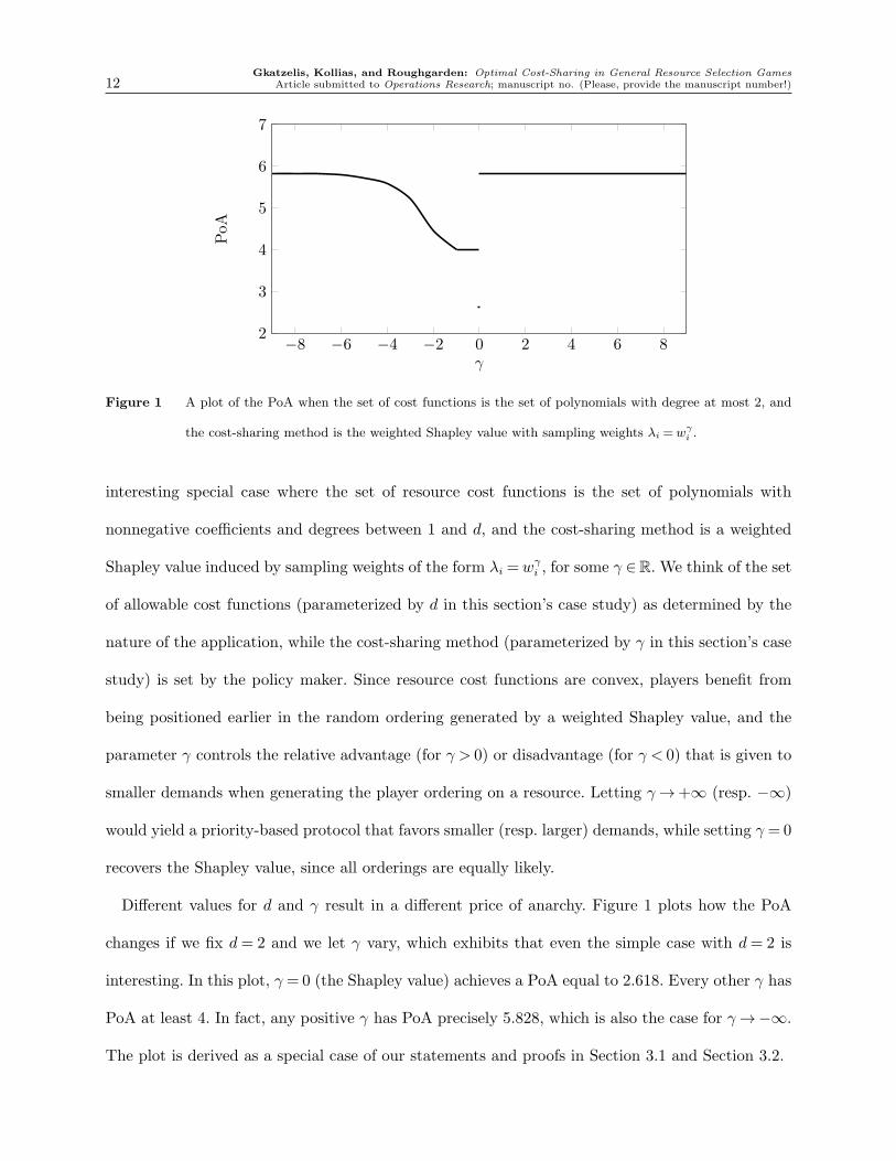
Figure 1 A plot of the PoA when the set of cost functions is the set of polynomials with degree at most 2, and

the cost-sharing method is the weighted Shapley value with sampling weights λi =wγi .

interesting special case where the set of resource cost functions is the set of polynomials with

nonnegative coefficients and degrees between 1 and d, and the cost-sharing method is a weighted

Shapley value induced by sampling weights of the form λi =wγi , for some γ ∈R. We think of the set

of allowable cost functions (parameterized by d in this section’s case study) as determined by the

nature of the application, while the cost-sharing method (parameterized by γ in this section’s case

study) is set by the policy maker. Since resource cost functions are convex, players benefit from

being positioned earlier in the random ordering generated by a weighted Shapley value, and the

parameter γ controls the relative advantage (for γ > 0) or disadvantage (for γ < 0) that is given to

smaller demands when generating the player ordering on a resource. Letting γ→+∞ (resp. −∞)

would yield a priority-based protocol that favors smaller (resp. larger) demands, while setting γ = 0

recovers the Shapley value, since all orderings are equally likely.

Different values for d and γ result in a different price of anarchy. Figure 1 plots how the PoA

changes if we fix d= 2 and we let γ vary, which exhibits that even the simple case with d= 2 is

interesting. In this plot, γ = 0 (the Shapley value) achieves a PoA equal to 2.618. Every other γ has

PoA at least 4. In fact, any positive γ has PoA precisely 5.828, which is also the case for γ→−∞.

The plot is derived as a special case of our statements and proofs in Section 3.1 and Section 3.2.



3.1. PoA Lower Bounds

Let Ξγ be a weighted Shapley value induced by sampling weights of the form λi =wγi . Also, let Cd

denote the set of polynomials with nonnegative coefficients and degrees between 1 and d. In this

section, we prove the following theorem.

Theorem 1 (Optimal parameterized weighted Shapley value for polynomials). For

cost functions in Cd, the Shapley value is optimal among all the cost-sharing methods Ξγ, i.e.,

argminγ

PoA(Cd,Ξγ) = 0

As we explained earlier, the γ = 0 case corresponds to the Shapley value (since all orderings

of the players on a resource have the same likelihood). In Kollias and Roughgarden (2011), it is

shown that the PoA of the Shapley value, when the cost functions are drawn from Cd, is equal

to χdd ≈ (0.9 · d)d, where χd is the largest root of 3 · xd − 1− (x+1)d. Our lower bounds show that

any γ 6= 0 results in a PoA larger than χdd.

Lemma 1 (Lower bound for polynomials and γ > 0). For positive values of γ:

PoA(Cd,Ξγ) ≥

(

21/d − 1)−d

≈ (1.4 · d)d.

As we prove in Theorem 2, this lower bound is in fact tight.

Lemma 2 (Lower bound for polynomials and γ < 0). For negative values of γ:

PoA(Cd,Ξγ) ≥ dd.

We prove an even stronger, but more complicated, lower bound for γ < 0 in Lemma 3 in the

electronic companion. From Lemma 1 and Lemma 2, we get the following theorem, which is the

main result of this section and an early indication of the general optimality of the Shapley value

among admissible cost-sharing methods.



3.2. PoA Upper Bounds

We first present an upper bound that applies to all weighted Shapley values (not only the ones

parameterized by γ), for games with polynomial cost functions of maximum degree d.

Theorem 2 (Upper bound for polynomials). For any admissible cost-sharing method Ξ:

PoA(Cd,Ξ) ≤(

21/d − 1)−d

≈ (1.4 · d)d.

Proof. Consider a game (N,R,A,w,Cd,Ξ). Let A be a PNE of the game and A∗ the optimal

outcome. For the total cost of A, we get:

Q(A) =∑

r∈R

Cr(lr(A)) =∑

r∈R

∑

i∈N

ξi,r(A) =∑

i∈N

∑

r∈Ai

ξi,r(A) ≤∑

i∈N

∑

r∈A∗

i

ξi,r(A∗i ,A−i). (9)

The inequality follows from the equilibrium condition (1). Note that the cost share of any player

on any resource, when the cost-sharing method is a weighted Shapley value and the resource costs

are convex, is upper bounded by the increase that would be caused on the joint resource cost, if

that player were to be the last in the ordering. This means that for every r ∈A∗i , we get:

ξi,r(A∗i ,A−i)≤Cr(lr(A

∗i ,A−i))−Cr(lr(A

∗i ,A−i)−wi)≤Cr(lr(A)+wi)−Cr(lr(A)). (10)

Combining (9) with (10), we get:

Q(A) ≤∑

i∈N

∑

r∈A∗

i

Cr(lr(A)+wi)−Cr(lr(A)) (11)

=∑

r∈R

∑

i∈Sr(A∗)

Cr(lr(A)+wi)−Cr(lr(A)) (12)

≤∑

r∈R

Cr(lr(A)+ lr(A∗))−Cr(lr(A)). (13)

The last inequality follows by convexity of the expression as a function of wi. We now claim that

the following is true, for any x, y ∈R, and d≥ 1:

(x+ y)d −xd ≤ λ · yd + µ ·xd, (14)

with

λ= 2(d−1)/d ·(

21/d − 1)−(d−1)

and µ= 2(d−1)/d − 1. (15)



We can verify this as follows. Note that, without loss of generality, we can set y = 1 (equivalent

to dividing both sides of (14) with yd and renaming x/y to x). We can then see that the value

of x that maximizes (x+ 1)d − µ · xd is x= 1/(21/d − 1), for which inequality (14) is tight. Also,

note that the expressions for λ and µ are increasing as functions of d, which implies that the given

values for degree d, satisfy (14) for smaller degrees as well. This means we can combine (13), (14),

and (15), to get:

Q(A) ≤∑

r∈R

λ ·Cr(lr(A∗))+ µ ·Cr(lr(A)) = λ ·Q(A∗)+ µ ·Q(A). (16)

Rearranging, we get Q(A)/Q(A∗)≤ λ/(µ+1) =(

21/d − 1)−d

. �

We prove a stronger, though more complicated, upper bound for γ < 0 in Lemma 4 in the

electronic companion.

4. General Convex Cost Functions and General Weighted Shapley Values

This section builds up to our main result. First we extend the results of Section 3 to general

weighted Shapley values (not just those of the form λi =wγi ) and polynomial cost functions and,

subsequently, we prove optimality of the Shapley value in games that draw resource costs from

arbitrary sets of allowable cost functions that satisfy the following conditions: cost functions are

positive, increasing, convex, assign 0 cost to 0 demand, and the cost function set is closed under

dilation (and scaling).

In general, a weighted Shapley value has the power to determine a player’s sampling weight as

a function of her identity and demand. Hence, we suppose the description of a weighted Shapley

value is given to us as a collection of functions, one for each player identity, that map a demand

to a sampling weight. We make the following mild technical assumptions: (a) the sampling weight

functions are continuous, i.e., slightly perturbing a player’s demand, also slightly perturbs her

sampling weight and (b) the limit of the sampling weight functions at 0 exists.

Consider a very large population of players N and for every i ∈ N , call λi(·) the function

that outputs the sampling weight of player i, given her demand. There are three cases: (i) the



limit limw→0 λi(w) is a positive constant for at least |N |/3 identities i (not necessarily the same

positive constant for all), (ii) the same limit is +∞ for at least |N |/3 identities, or (iii) the same

limit is 0 for at least |N |/3 identities. Fix a very large set N and admissible cost-sharing method Ξ.

If Ξ falls under case (i) we call it balanced with respect to N , if it falls under case (ii) we call it small-

demand-punishing with respect to N , and if it falls under case (iii) we call it small-demand-favoring

with respect to N . We then get the following:

Theorem 3 (Optimal admissible cost-sharing method for polynomials). Let Ξ be any

admissible cost-sharing method:

1. If Ξ is balanced with respect to N , then PoA(Cd,Ξ) ≥ χdd ≈ 0.9 · d.

2. If Ξ is small-demand-punishing with respect to N , then PoA(Cd,Ξ) ≥ dd.

3. If Ξ is small-demand-favoring with respect to N , then PoA(Cd,Ξ) ≥ (21/d−1)−d ≈ (1.4 ·d)d.

It follows that the PoA of χdd achieved by the Shapley value is optimal.

We now generalize this result to get our main theorem:

Theorem 4 (Optimal admissible cost-sharing method for convex functions). Let ΞSV

denote the Shapley value and Ξ any admissible cost-sharing method. Also, let C denote any given

set of positive, increasing, and convex cost functions which assign 0 cost to 0 demand, which has the

property that if C(x)∈ C, then a ·C(b ·x)∈ C for any positive a, b. Then, PoA(C,ΞSV)≤ PoA(C,Ξ).

5. Discussion and Open Questions

This paper studies the interactions among self-interested agents who place demands on shared

resources which incur a congestion-dependent cost. In this setting, and when the cost functions are

convex, we make the case that distributing the generated cost among the participants using the

Shapley value leads to the best price of anarchy among all cost-sharing methods possessing certain

desirable properties: budget-balance, stability, and locality. It is worth noting that the upper bounds

on the price of anarchy make use of the (λ,µ)-smoothness framework of Roughgarden (2009), which

implies that these bounds are robust, i.e., they hold even for equilibrium concepts more general



than the pure Nash equilibrium (e.g., the mixed Nash equilibrium) which are guaranteed to exist.

As a result, the optimality of the Shapley value holds much more generally.

Our prescribed properties of budget-balance, stability, and locality are important in our moti-

vating applications. However, understanding the design space beyond such admissible cost-sharing

methods is an interesting question. For example, various ways in which the locality property can

be relaxed are discussed in von Falkenhausen and Harks (2013). Violating the stability requirement

implies dropping the existence of a pure Nash equilibrium and it may, hence, induce unappealing

gaming behavior. Nevertheless, we briefly addressed this question in a recently announced extended

abstract (Gkatzelis et al. (2014)). In particular, for polynomial cost functions of maximum degree d,

we prove that the proportional sharing method, which is known to violate the stability property,

achieves a robust price of anarchy that is essentially optimal among all cost-sharing methods that

satisfy the other two properties.

Maybe the most interesting extension would be to relax the budget-balance requirement.

Gopalakrishnan et al. (2013) show that, as long as the stability property is enforced, the cost-

sharing method will necessarily distribute a total cost according to some weighted Shapley value,

although the cost being distributed need not be the same as the generated cost anymore. The

cost-sharing method within this class that is arguably the most natural and well studied one is

the marginal contribution, according to which each player suffers a cost equal to her marginal

contribution in the total cost. For convex cost functions, like the ones that we considered in this

paper, this method charges the players a total cost that is higher than the cost that their use of

the resources generated. In Gkatzelis et al. (2014) we also show that, for polynomial cost functions

of maximum degree d, the marginal contribution method leads to PoA worse than that of any

weighted Shapley value.

Finally, another interesting open problem is to identify the optimal cost-sharing method in games

that are symmetric, i.e., all the players have the same strategy set.



References

Abed, Fidaa, Chien-Chung Huang. 2012. Preemptive coordination mechanisms for unrelated machines. Leah

Epstein, Paolo Ferragina, eds., Algorithms ESA 2012 , Lecture Notes in Computer Science, vol. 7501.

Springer Berlin Heidelberg, 12–23.

Anshelevich, E., A. Dasgupta, J. Kleinberg, E. Tardos, T. Wexler, T. Roughgarden. 2008. The price of

stability for network design with fair cost allocation. SIAM Journal on Computing 38(4) 1602–1623.

Awerbuch, B., Y. Azar, L. Epstein. 2005. The price of routing unsplittable flow. Proceedings of the 37th

Annual ACM Symposium on Theory of Computing (STOC). 57–66.

Azar, Yossi, Kamal Jain, Vahab Mirrokni. 2008. (almost) optimal coordination mechanisms for unrelated

machine scheduling. Proceedings of the Nineteenth Annual ACM-SIAM Symposium on Discrete Algo-

rithms . SODA ’08, Society for Industrial and Applied Mathematics, Philadelphia, PA, USA, 323–332.

Bhattacharya, Sayan, Sungjin Im, Janardhan Kulkarni, Kamesh Munagala. 2014. Coordination mechanisms

from (almost) all scheduling policies. Proceedings of the 5th Conference on Innovations in Theoretical

Computer Science. ITCS ’14, ACM, New York, NY, USA, 121–134.

Bhawalkar, K., M. Gairing, T. Roughgarden. 2010. Weighted congestion games: Price of anarchy, universal

worst-case examples, and tightness. Proceedings of the 18th Annual European Symposium on Algorithms

(ESA), vol. 2. 17–28.

Bhawalkar, Kshipra, Tim Roughgarden. 2012. Simultaneous single-item auctions. WINE . 337–349.

Caragiannis, Ioannis. 2009. Efficient coordination mechanisms for unrelated machine scheduling. Proceed-

ings of the Twentieth Annual ACM-SIAM Symposium on Discrete Algorithms . SODA ’09, Society for

Industrial and Applied Mathematics, Philadelphia, PA, USA, 815–824.

Chen, H., T. Roughgarden, G. Valiant. 2010. Designing network protocols for good equilibria. SIAM Journal

on Computing 39(5) 1799–1832.

Christodoulou, George, Elias Koutsoupias, Akash Nanavati. 2009. Coordination mechanisms. Theor. Comput.

Sci. 410(36) 3327–3336.

Christodoulou, Giorgos, Kurt Mehlhorn, Evangelia Pyrga. 2014. Improving the price of anarchy for selfish

routing via coordination mechanisms. Algorithmica 69(3) 619–640.



Coffman Jr., E. G., I. Mitrani. 1980. A characterization of waiting time performance realizable by single-

server queues. Operations Research 28(3) pp. 810–821.

Cole, Richard, Jos R. Correa, Vasilis Gkatzelis, Vahab Mirrokni, Neil Olver. 2013. Decentralized utilitarian

mechanisms for scheduling games. Games and Economic Behavior (0) –.

Cominetti, Roberto, Jose R. Correa, Nicolas E. Stier Moses. 2009. The impact of oligopolistic competition

in networks. Operations Research 57(6) 1421–1437.

Fotakis, Dimitris, Paul G. Spirakis. 2008. Cost-balancing tolls for atomic network congestion games. Internet

Mathematics 5(4) 343–363.

Gairing, Martin, Florian Schoppmann. 2007. Total latency in singleton congestion games. Xiaotie Deng,

FanChung Graham, eds., Internet and Network Economics , Lecture Notes in Computer Science, vol.

4858. Springer Berlin Heidelberg, 381–387.

Gkatzelis, Vasilis, Konstantinos Kollias, Tim Roughgarden. 2014. Optimal cost-sharing in weighted conges-

tion games. Web and Internet Economics - 10th International Conference, WINE .

Gopalakrishnan, Ragavendran, Jason R. Marden, Adam Wierman. 2013. Potential games are necessary to

ensure pure nash equilibria in cost sharing games. Proceedings of the Fourteenth ACM Conference on

Electronic Commerce. EC ’13, ACM, New York, NY, USA, 563–564.

Harks, T., M. Klimm. 2012. On the existence of pure Nash equilibria in weighted congestion games. Math-

ematics of Operations Research 37(3) 419–436.

Harks, T., M. Klimm, R. H. Mohring. 2011. Characterizing the existence of potential functions in weighted

congestion games. Theory of Computing Systems 49(1) 46–70.

Harks, Tobias, Konstantin Miller. 2011. The worst-case efficiency of cost sharing methods in resource allo-

cation games. Operations Research 59(6) 1491–1503.

Haviv, Moshe, Tim Roughgarden. 2007. The price of anarchy in an exponential multi-server. Oper. Res.

Lett. 35(4) 421–426.

Immorlica, Nicole, Li (Erran) Li, Vahab S. Mirrokni, Andreas S. Schulz. 2009. Coordination mechanisms for

selfish scheduling. Theor. Comput. Sci. 410(17) 1589–1598.



Kollias, Konstantinos. 2013. Nonpreemptive coordination mechanisms for identical machines. Theory of

Computing Systems 53(3) 424–440. doi:10.1007/s00224-012-9429-9.

Kollias, Konstantinos, Tim Roughgarden. 2011. Restoring pure equilibria to weighted congestion games.

Automata, Languages and Programming , Lecture Notes in Computer Science, vol. 6756. Springer Berlin

Heidelberg, 539–551.

Lucier, Brendan, Allan Borodin. 2010. Price of anarchy for greedy auctions. SODA. 537–553.

Marden, J. R., A. Wierman. 2013. Distributed welfare games. Operations Research 61(1) 155–168.

Milchtaich, I. 1996. Congestion games with player-specific payoff functions. Games and Economic Behavior

13(1) 111–124.

Monderer, D., L. S. Shapley. 1996. Potential games. Games and Economic Behavior 14(1) 124–143.

Mosk-Aoyama, Damon, Tim Roughgarden. 2009. Worst-case efficiency analysis of queueing disciplines.

ICALP (2). 546–557.

Moulin, H. 2008. The price of anarchy of serial, average and incremental cost sharing. Economic Theory

36(3) 379–405.

Moulin, Herv, Scott Shenker. 2001. Strategyproof sharing of submodular costs:budget balance versus effi-

ciency. Economic Theory 18(3) 511–533.

Rosenthal, R. W. 1973a. A class of games possessing pure-strategy Nash equilibria. International Journal

of Game Theory 2(1) 65–67.

Rosenthal, R. W. 1973b. The network equilibrium problem in integers. Networks 3(1) 53–59.

Roughgarden, T. 2009. Intrinsic robustness of the price of anarchy. 41st ACM Symposium on Theory of

Computing (STOC). 513–522.

Roughgarden, T., E. Tardos. 2002. How bad is selfish routing? Journal of the ACM 49(2) 236–259.

Shapley, L. S. 1953. Additive and non-additive set functions. Ph.D. thesis, Department of Mathematics,

Princeton University.

Shenker, S. J. 1995. Making greed work in networks: A game-theoretic analysis of switch service disciplines.

IEEE/ACM Transactions on Networking 3(6) 819–831.



Syrgkanis, Vasilis, Eva Tardos. 2013. Composable and efficient mechanisms. STOC . 211–220.

von Falkenhausen, Philipp, Tobias Harks. 2013. Optimal cost sharing for resource selection games. Math.

Oper. Res. 38(1) 184–208.



Proofs of Statements

6. Proof of Lemma 1.

Lemma 1. For positive values of γ:

PoA(Cd,Ξγ) ≥

(

21/d − 1)−d

≈ (1.4 · d)d

Proof. Define ρ= (21/d−1)−1 and let T be a set of ρ/ǫ players with demand ǫ each, where ǫ > 0

is an arbitrarily small parameter. Consider a player i with demand wi = 1 and suppose she uses

a resource r with cost function Cr(x) = xd with the players in T , while the cost-sharing rule is

our Ξγ . We now argue that, as we let ǫ→ 0, the cost share of i in r becomes (ρ+1)d−ρd. Consider

the probability p that i is not among the last δ · |T | players of the random ordering generated by

our sampling weights (i.e., i is not among the first δ · |T | players sampled), for some δ < 1. This

probability is upper bounded by the probability that i is not drawn, using our sampling weights,

among everyone in T ∪ {i}, δ · |T |= δ · ρ/ǫ times. Note that the sampling weight of i is 1 and the

total sampling weight of the players in T is ρ · ǫγ−1. Hence, if γ ≥ 1, we get:

p≤

(

1−1

1+ ρ · ǫγ−1

)δ·ρ/ǫ

≤

(

1−1

1+ ρ

)δ·ρ/ǫ

, (17)

which goes to 0 as ǫ→ 0. Similarly, if γ < 1, we get:

p≤

(

1−1

1+ ρ · ǫγ−1

)δ·ρ/ǫ

≤ exp

(

−δ ·ρ

ǫ·

1

1+ ρ · ǫγ−1

)

= exp

(

−δ · ρ ·ǫ−γ

ǫ1−γ + ρ

)

, (18)

which always goes to 0 as ǫ→ 0, for any arbitrarily small δ > 0. Then, by letting δ→ 0, our claim

that the cost share of i is (ρ+ 1)d − ρd follows by (3). Similarly, it follows that if a player with

demand w shares a resource with cost function a ·xd with ρ/ǫ players with demand w · ǫ each, her

cost share will be a ·wd · ((ρ+ 1)d − ρd) (since scaling the cost function and the player demands

does not change the fractions of the cost that are assigned to the players), which, for our choice

of ρ is equal to a ·wd · ρd.

Using facts from the previous paragraph as building blocks, we construct a

game (N,R,A,w,Cd,Ξγ), such that the total cost in the worst equilibrium is ρd times the optimal.



Suppose our resources are organized in a tree graph G = (R,E), where each vertex corresponds

to a resource. There is a one-to-one mapping between the set of edges of the tree, E, and the

set of players of the game, N . The player i, that corresponds to edge e = (r, r′), has strategy

set Ai = {{r},{r′}}, i.e., she must choose one of the two endpoints of her designated edge. Tree G

has branching factor ρ/ǫ and l levels, with the root positioned at level 1 and the leaves positioned

at level l.

Player demands. The demand of every player (edge) between resources (vertices) at levels j

and j+1 of the tree is ǫj−1.

Cost functions. The cost function of any resource (vertex) at level j = 1,2, . . . , l− 1, is:

Cj(x) =

(

1

ρ · ǫd−1

)j−1

·xd. (19)

The cost functions of any resource (vertex) at level l is equal to:

C l(x) =ρd−l+1

ǫ(d−1)·(l−1)·xd. (20)

PNE. Let A be the outcome that has all players play the resource closer to the root. We claim

that this outcome is a PNE. The cost of every player, using a resource at level j < l, in A, is (ρ/ǫ)d−j.

If one of the players that are adjacent to the leaves were to switch to her other strategy (play

the leaf resource), she would incur a cost equal to (ρ/ǫ)d−l+1, which is the same as the one she

has in A. Consider any other player and her potential deviation from the resource at level j, to

the resource at level j + 1. By the analysis in the first paragraph of this proof (she would be a

player with demand ǫj−1 sharing a resource with ρ/ǫ players with demand ǫj), her cost would

be (ρ · ǫd−1)j · ǫd·(j−1) ·ρd = (ρ/ǫ)d−j, which is her current cost in A. This proves that the equilibrium

condition (1) holds for all players in A.

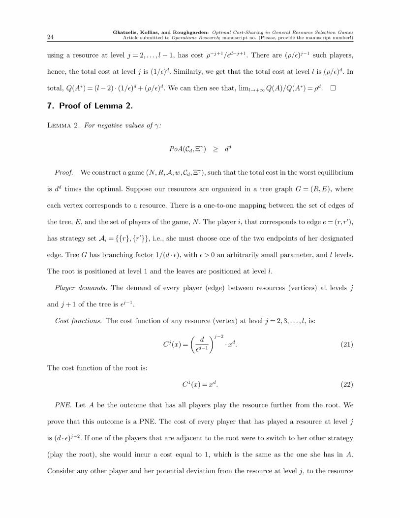
PoA. As we have shown, every player using a resource at level j has cost (ρ/ǫ)d−j in A. There

are (ρ/ǫ)j such players, which implies the total cost of A isQ(A) = (l−1) ·(ρ/ǫ)d, since there are l−1

levels of nonempty resources, and every level has the same total cost, (ρ/ǫ)d. Now, let A∗ be the

outcome that has all players play the resource further from the root. In this outcome, every player



using a resource at level j = 2, . . . , l − 1, has cost ρ−j+1/ǫd−j+1. There are (ρ/ǫ)j−1 such players,

hence, the total cost at level j is (1/ǫ)d. Similarly, we get that the total cost at level l is (ρ/ǫ)d. In

total, Q(A∗) = (l− 2) · (1/ǫ)d +(ρ/ǫ)d. We can then see that, liml→+∞Q(A)/Q(A∗) = ρd. �

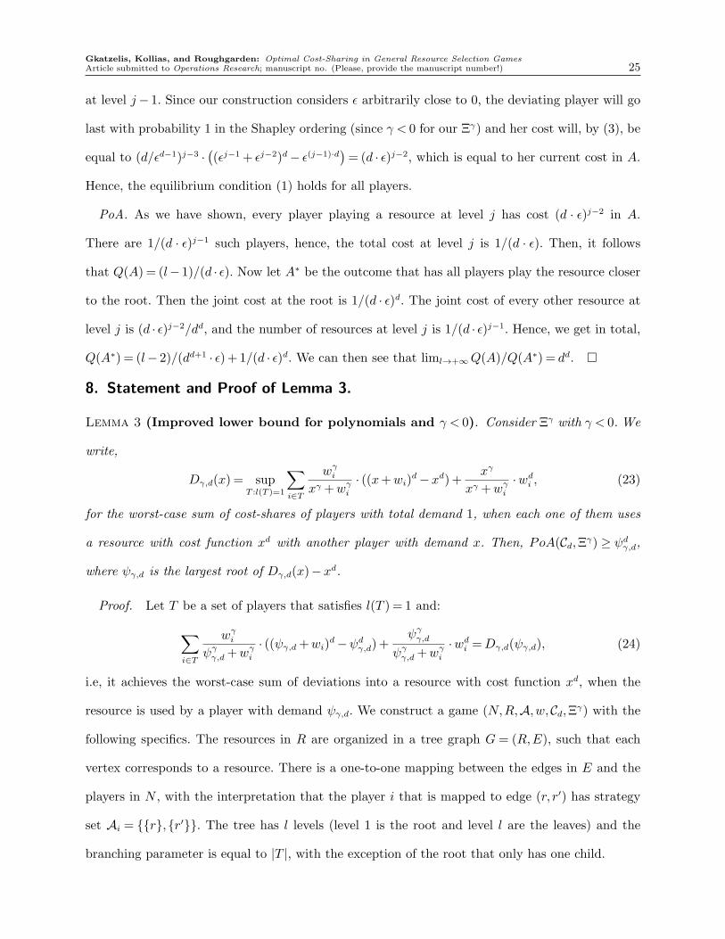
7. Proof of Lemma 2.

Lemma 2. For negative values of γ:

PoA(Cd,Ξγ) ≥ dd

Proof. We construct a game (N,R,A,w,Cd,Ξγ), such that the total cost in the worst equilibrium

is dd times the optimal. Suppose our resources are organized in a tree graph G = (R,E), where

each vertex corresponds to a resource. There is a one-to-one mapping between the set of edges of

the tree, E, and the set of players of the game, N . The player i, that corresponds to edge e= (r, r′),

has strategy set Ai = {{r},{r′}}, i.e., she must choose one of the two endpoints of her designated

edge. Tree G has branching factor 1/(d · ǫ), with ǫ > 0 an arbitrarily small parameter, and l levels.

The root is positioned at level 1 and the leaves are positioned at level l.

Player demands. The demand of every player (edge) between resources (vertices) at levels j

and j+1 of the tree is ǫj−1.

Cost functions. The cost function of any resource (vertex) at level j = 2,3, . . . , l, is:

Cj(x) =

(

d

ǫd−1

)j−2

·xd. (21)

The cost function of the root is:

C1(x) = xd. (22)

PNE. Let A be the outcome that has all players play the resource further from the root. We

prove that this outcome is a PNE. The cost of every player that has played a resource at level j

is (d · ǫ)j−2. If one of the players that are adjacent to the root were to switch to her other strategy

(play the root), she would incur a cost equal to 1, which is the same as the one she has in A.

Consider any other player and her potential deviation from the resource at level j, to the resource



at level j− 1. Since our construction considers ǫ arbitrarily close to 0, the deviating player will go

last with probability 1 in the Shapley ordering (since γ < 0 for our Ξγ) and her cost will, by (3), be

equal to (d/ǫd−1)j−3 ·(

(ǫj−1 + ǫj−2)d − ǫ(j−1)·d)

= (d · ǫ)j−2, which is equal to her current cost in A.

Hence, the equilibrium condition (1) holds for all players.

PoA. As we have shown, every player playing a resource at level j has cost (d · ǫ)j−2 in A.

There are 1/(d · ǫ)j−1 such players, hence, the total cost at level j is 1/(d · ǫ). Then, it follows

that Q(A) = (l− 1)/(d · ǫ). Now let A∗ be the outcome that has all players play the resource closer

to the root. Then the joint cost at the root is 1/(d · ǫ)d. The joint cost of every other resource at

level j is (d · ǫ)j−2/dd, and the number of resources at level j is 1/(d · ǫ)j−1. Hence, we get in total,

Q(A∗) = (l− 2)/(dd+1 · ǫ)+ 1/(d · ǫ)d. We can then see that liml→+∞Q(A)/Q(A∗) = dd. �

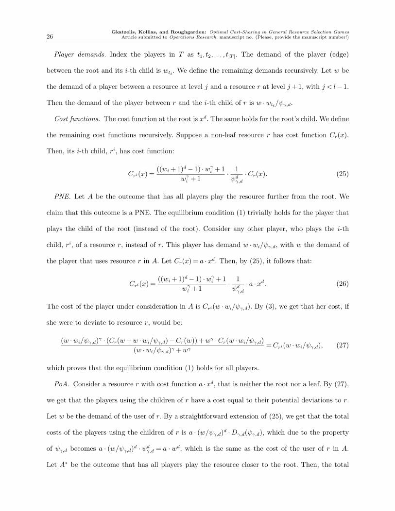
8. Statement and Proof of Lemma 3.

Lemma 3 (Improved lower bound for polynomials and γ < 0). Consider Ξγ with γ < 0. We

write,

Dγ,d(x) = supT :l(T )=1

∑

i∈T

wγi

xγ +wγi

· ((x+wi)d −xd)+

xγ

xγ +wγi

·wdi , (23)

for the worst-case sum of cost-shares of players with total demand 1, when each one of them uses

a resource with cost function xd with another player with demand x. Then, PoA(Cd,Ξγ) ≥ ψd

γ,d,

where ψγ,d is the largest root of Dγ,d(x)−xd.

Proof. Let T be a set of players that satisfies l(T ) = 1 and:

∑

i∈T

wγi

ψγγ,d +wγ

i

· ((ψγ,d +wi)d −ψd

γ,d)+ψγ

γ,d

ψγγ,d +wγ

i

·wdi =Dγ,d(ψγ,d), (24)

i.e, it achieves the worst-case sum of deviations into a resource with cost function xd, when the

resource is used by a player with demand ψγ,d. We construct a game (N,R,A,w,Cd,Ξγ) with the

following specifics. The resources in R are organized in a tree graph G = (R,E), such that each

vertex corresponds to a resource. There is a one-to-one mapping between the edges in E and the

players in N , with the interpretation that the player i that is mapped to edge (r, r′) has strategy

set Ai = {{r},{r′}}. The tree has l levels (level 1 is the root and level l are the leaves) and the

branching parameter is equal to |T |, with the exception of the root that only has one child.



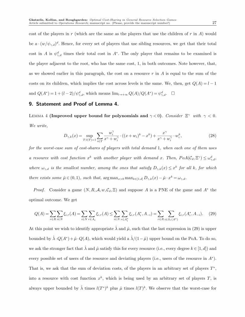
Player demands. Index the players in T as t1, t2, . . . , t|T |. The demand of the player (edge)

between the root and its i-th child is wti . We define the remaining demands recursively. Let w be

the demand of a player between a resource at level j and a resource r at level j+1, with j < l− 1.

Then the demand of the player between r and the i-th child of r is w ·wti/ψγ,d.

Cost functions. The cost function at the root is xd. The same holds for the root’s child. We define

the remaining cost functions recursively. Suppose a non-leaf resource r has cost function Cr(x).

Then, its i-th child, ri, has cost function:

Cri(x) =((wi +1)d − 1) ·wγ

i +1

wγi +1

·1

ψdγ,d

·Cr(x). (25)


claim that this outcome is a PNE. The equilibrium condition (1) trivially holds for the player that

plays the child of the root (instead of the root). Consider any other player, who plays the i-th

child, ri, of a resource r, instead of r. This player has demand w ·wi/ψγ,d, with w the demand of

the player that uses resource r in A. Let Cr(x) = a ·xd. Then, by (25), it follows that:

Cri(x) =((wi +1)d − 1) ·wγ

i +1

wγi +1

·1

ψdγ,d

· a ·xd. (26)

The cost of the player under consideration in A is Cri(w ·wi/ψγ,d). By (3), we get that her cost, if

she were to deviate to resource r, would be:

(w ·wi/ψγ,d)γ · (Cr(w+w ·wi/ψγ,d)−Cr(w))+wγ ·Cr(w ·wi/ψγ,d)

(w ·wi/ψγ,d)γ +wγ=Cri(w ·wi/ψγ,d), (27)

which proves that the equilibrium condition (1) holds for all players.

PoA. Consider a resource r with cost function a ·xd, that is neither the root nor a leaf. By (27),

we get that the players using the children of r have a cost equal to their potential deviations to r.

Let w be the demand of the user of r. By a straightforward extension of (25), we get that the total

costs of the players using the children of r is a · (w/ψγ,d)d ·Dγ,d(ψγ,d), which due to the property

of ψγ,d becomes a · (w/ψγ,d)d · ψd

γ,d = a · wd, which is the same as the cost of the user of r in A.

Let A∗ be the outcome that has all players play the resource closer to the root. Then, the total



cost of the players in r (which are the same as the players that use the children of r in A) would

be a · (w/ψγ,d)d. Hence, for every set of players that use sibling resources, we get that their total

cost in A is ψdγ,d times their total cost in A∗. The only player that remains to be examined is

the player adjacent to the root, who has the same cost, 1, in both outcomes. Note however, that,

as we showed earlier in this paragraph, the cost on a resource r in A is equal to the sum of the

costs on its children, which implies the cost across levels is the same. We, then, get Q(A) = l− 1

and Q(A∗) = 1+ (l− 2)/ψdγ,d, which means liml→+∞Q(A)/Q(A∗) =ψd

γ,d. �

9. Statement and Proof of Lemma 4.

Lemma 4 (Improved upper bound for polynomials and γ < 0). Consider Ξγ with γ < 0.

We write,

Dγ,k(x) = supT :l(T )=1

∑

i∈T

wγi

xγ +wγi

· ((x+wi)k −xk)+

xγ

xγ +wγi

·wki , (28)

for the worst-case sum of cost-shares of players with total demand 1, when each one of them uses

a resource with cost function xk with another player with demand x. Then, PoA(Cd,Ξγ) ≤ ωd

γ,d,

where ωγ,d is the smallest number, among the ones that satisfy Dγ,k(x) ≤ xk for all k, for which

there exists some µ∈ (0,1), such that, argmaxx>0maxk∈[1,d]Dγ,k(x)− µ ·xk = ωγ,d.

Proof. Consider a game (N,R,A,w,Cd,Ξ) and suppose A is a PNE of the game and A∗ the

optimal outcome. We get

Q(A) =∑

r∈R

∑

i∈N

ξi,r(A) =∑

i∈N

∑

r∈Ai

ξi,r(A)≤∑

i∈N

∑

r∈A∗

i

ξi,r(A∗i ,A−i) =

∑

r∈R

∑

i∈Sr(A∗)

ξi,r(A∗i ,A−i). (29)

At this point we wish to identify appropriate λ and µ, such that the last expression in (29) is upper

bounded by λ ·Q(A∗)+ µ ·Q(A), which would yield a λ/(1− µ) upper bound on the PoA. To do so,

we ask the stronger fact that λ and µ satisfy this for every resource (i.e., every degree k ∈ [1, d]) and

every possible set of users of the resource and deviating players (i.e., users of the resource in A∗).

That is, we ask that the sum of deviation costs, of the players in an arbitrary set of players T ∗,

into a resource with cost function xk, which is being used by an arbitrary set of players T , is

always upper bounded by λ times l(T ∗)k plus µ times l(T )k. We observe that the worst-case for



the deviating players (hence, the worst-case for our upper bound) is when T is a single player,

because γ < 0 (there is higher probability that the demand already in the resource is earlier than

the deviating player in the Shapley ordering). In short, if λ and µ satisfy, for every k ∈ [1, d],

x, y > 0, and every T ∗ such that l(T ∗) = x:

∑

i∈T∗

wγi

wγi +xγ

·(

(wi +x)k −xk)

+xγ

wγi +xγ

·wki ≤ λ · yk + µ ·xk, (30)

then, combining with (29), we get a λ/(1− µ) upper bound on the PoA. We can see that scaling

the player demands does not impact the constraint (30). Hence, by considering x and 1, as opposed

to x and y, and by considering only the worst-case T ∗, we can rewrite (30) as:

Dγ,k(x)≤ λ+ µ ·xk. (31)

We choose µ to be the value that lets ωγ,d be used as the worst-case value for x in (31). Then we

choose λ such as to make this worst-case for (31) tight. Then, from (31), we get:

Dγ,k(ωγ,d) = λ+ µ ·ωkγ,d ⇒

λ

1− µ=Dγ,k(ωγ,d)− µ ·ωk

γ,d

1− µ≤ ωk

γ,d ≤ ωdγ,d, (32)

where the final inequality follows from the properties of ωγ,d. �

Typically, and for the vast majority of γ, d pairs, this upper bound matches the lower bound

from Lemma 3. It is possible that there exist rare pathological cases, for which the two bounds do

not match, however, even finding one such γ, d pair is a difficult task.

10. Proof of Theorem 3.

Theorem 3. Let Ξ be any admissible cost-sharing method and N an arbitrarily large set of players:

1. If Ξ is balanced with respect to N , then PoA(Cd,Ξ) ≥ χdd ≈ 0.9 · d.

2. If Ξ is small-demand-punishing with respect to N , then PoA(Cd,Ξ) ≥ dd.

3. If Ξ is small-demand-favoring with respect to N , then PoA(Cd,Ξ) ≥ (21/d−1)−d ≈ (1.4 ·d)d.

It then follows that the PoA of χdd achieved by the Shapley value is optimal.

We prove the theorem via the following sequence of lemmas.



Lemma 5. Let Ξ be a weighted Shapley value that is balanced with respect to N , an arbitrarily large

set of players. With Cd the set of polynomials with nonnegative coefficients and degrees between 1

and d, we get that PoA(Cd,Ξ)≥ χdd.

Proof. We will construct a game (N,R,A,w,Cd,Ξ) such that the worst equilibrium cost is χdd

times the optimal cost. Focus on the subset of players whose designated sampling weight function

has a positive and finite limit at 0. In this subset, find a sequence of l players, i1, i2, . . . , il, such

that, if the limit at 0 of the sampling weight function for player i is λ0i , then λ

0i1≥ λ0

i2≥ . . .≥ λ0

il.

Such a sequence trivially exists. Now, suppose ǫ is a very small number, such that the value of

the sampling weight function of player i for any demand at most ǫ is arbitrarily close to λ0i . By

continuity, such an ǫ exists. The resources are arranged on a line as r1, r2, . . . , rl+1, and there is an

extra resource r0, which does not belong on the line. Each Player ij of the sequence we identified

at the start of the proof has strategy set Aij = {{rj},{rj+1}}, i.e., she must pick one of rj and rj+1.

All other players in N have only one possible strategy, which is to play r0.

Player demands. The demand of Player ij , for j = 1,2, . . . , l, is ǫ/χjd. The demand of any other

player in N is 0.

Cost functions. The cost function of r1 is xd and the cost function of rj, for j = 2, . . . , l, is χ

d·(j−1)d ·

xd. The cost function of r0 is xd.

PNE. Let A be the outcome where Player ij plays resource rj+1, for j = 1,2, . . . , l. The equi-

librium condition trivially holds for all players using r0 (since they have no other option) and for

Player i1 (since r1 and r2 have the same cost). Every other player has cost (ǫ/χd)d in A. The cost

of her potential deviation is at least her Shapley value on the other resource (by the choice of the

sequence of players i1, i2, . . . , il in the beginning), which is also (ǫ/χd)d.

PoA. Let A∗ be the outcome that has Player ij play resource j, for j = 1,2, . . . , l. We observe

that Q(A) = l · (ǫ/χd)d and Q(A∗) = (ǫ/χd)

d + (l− 1) · (ǫ/χ2d)

d. Then liml→+∞Q(A)/Q(A∗) = χdd.

Note that we can let l grow to infinity, since Ξ is balanced with respect to N and N is arbitrarily

large. �



Lemma 6. Let Ξ be a weighted Shapley value that is small-demand-punishing with respect to N ,

an arbitrarily large set of players. With Cd the set of polynomials with nonnegative coefficients and

degrees between 1 and d, we get that PoA(Cd,Ξ)≥ dd.

Proof. We construct a game (N,R,A,w,Cd,Ξ) such that the cost of the worst equilibrium is dd

times the cost of the optimal outcome. The resources in R are organized in a tree graph G =

(R\{r0},E), where each vertex corresponds to a resource, with the exception of a single resource r0,

which does not belong to the tree. The tree has l levels and the branching factor is 1/(d · ǫ), where ǫ

is an arbitrarily small parameter, with the exception of the root, which has only one child. Each

edge (r, r′)∈E corresponds to a distinct Player i∈N , who has strategy set Ai = {{r},{r′}}. Every

player from N that is not mapped to an edge, has playing r0 as her only available strategy.

Player placement and demands. Focus only on players such that their designated sampling weight

functions approach infinity as their demands approach 0. Since Ξ is small-demand-punishing with

respect to N and N is arbitrarily large, there is an infinite supply of such players. Fill the edges

of G with such players. As already stated, all other players will have r0 as their only strategy. All

players placed in r0 have demand 0. A player between levels j and j+1 of the tree has demand ǫj−1.

Cost functions. The cost function of any resource at level j = 2,3, . . . , l, is (d/ǫd−1)j−2 · xd. The

cost functions of the root is xd and the cost function of r0 is also xd.


prove that this outcome is a PNE. The cost of every player that has played a resource at level j

is (d · ǫ)j−2. If one of the players that are adjacent to the root were to switch to her other strategy

(play the root), she would incur a cost equal to 1, which is the same as the one she has in A.

Consider any other player and her potential deviation from the resource at level j, to the resource

at level j− 1. Since our construction considers ǫ arbitrarily close to 0, the deviating player will go

last with probability 1 in the Shapley ordering (since γ < 0 for our Ξγ) and her cost will, by (3), be

equal to (d/ǫd−1)j−3 ·(

(ǫj−1 + ǫj−2)d − ǫ(j−1)·d)

= (d · ǫ)j−2, which is equal to her current cost in A.

Hence, the equilibrium condition (1) holds for all players.



PoA. As we have shown, every player playing a resource at level j has cost (d · ǫ)j−2 in A.

There are 1/(d · ǫ)j−1 such players, hence, the total cost at level j is 1/(d · ǫ). Then, it follows

that Q(A) = (l− 1)/(d · ǫ). Now let A∗ be the outcome that has all players play the resource closer

to the root. Then the joint cost at the root is 1/(d · ǫ)d. The joint cost of every other resource at

level j is (d · ǫ)j−2/dd, and the number of resources at level j is 1/(d · ǫ)j−1. Hence, we get in total,

Q(A∗) = (l− 2)/(dd+1 · ǫ)+ 1/(d · ǫ)d. We can then see that liml→+∞Q(A)/Q(A∗) = dd. �

Lemma 7. Let Ξ be a weighted Shapley value that is small-demand-favoring with respect to N , an

arbitrarily large set of players. With Cd the set of polynomials with nonnegative coefficients and

degrees between 1 and d, we get that PoA(Cd,Ξ)≥ (21/d − 1)−d.

Proof. Let ρ= (21/d − 1)−1. We construct a game (N,R,A,w,Cd,Ξ) such that the cost of the

worst equilibrium is ρd times the cost of the optimal outcome. The resources are organized in a

tree graph G= (R \ {r0},E), which has a vertex for each resource, with the exception of a single

resource r0, which does not belong to the tree. The tree has l levels and the branching factor

is ρ/ǫ, where ǫ is an arbitrarily small parameter. Each edge (r, r′) ∈ E corresponds to a distinct

Player i ∈N , who has strategy set Ai = {{r},{r′}}. Every player from N that is not mapped to

an edge, has playing r0 as her only available strategy.

Player placement and demands. Focus only on players such that their designated sampling weight

functions goes to 0 as their demands approach 0. Since Ξ is small-demand-favoring with respect

to N and N is arbitrarily large, there is an infinite supply of such players. Fill the edges of G with

such players. All other players will have r0 as their only strategy. All players placed in r0 have

demand 0. A player between levels j and j+1 of the tree has demand ǫj−1.

Cost functions. The cost function at the root is xd. For levels 2,3, . . . , l− 1, we define the cost

functions recursively. Suppose the cost function of a resource r at level j < l − 2 is Cr(x) and

consider the player i that is between the resource and its child r′. Let A be the outcome that has all

players on the tree play the resource closer to the root. Suppose the fraction of the joint cost of r

in A that is covered by player i is αir. Then the cost function of resource r′ is Cr′(x) = αi

r ·Cr(x)/ǫd.



Finally, if the cost function of a resource r at level l − 1 is Cr(x), and the cost fraction that

is assigned to the player i between r and its child r′ in A is αir, then the cost function of r′

is Cr′(x) = αir · (ρ/ǫ)

d ·Cr(x).

PNE. Consider outcome A as in the previous paragraph. We will show that it is a PNE. Consider

a player i adjacent to a leaf. Let r be the resource that the player is using in A. Then her cost

is αir ·Cr(wi ·ρ/ǫ). If she were to deviate to the leaf resource, her cost would be αi

r · (ρ/ǫ)d ·Cr(wi).

We can easily verify that the two quantities are equal. Now consider any other player i that is

using a resource r at level j < l− 1. The cost of i in A is air ·Cr(wi · ρ/ǫ). If i deviates to the child

of r, her cost will be air · (Cr(wi · (1+ ρ))−Cr(wi · ρ))/ǫd (since, as we explained in Lemma 1, with

such sampling weights, the player’s cost share is as if she goes last in the Shapley ordering with

probability 1), which, by the fact that for our choice of ρ, (1+ρ)d−ρd = ρd, is equal to her current

cost in A. Hence, the equilibrium condition holds for all players.

PoA. The total cost of A is Q(A) = (l − 1) · (ρ/ǫ)d, since there are l − 1 levels of nonempty

resources, and every level has the same total cost, (ρ/ǫ)d, by the fact that∑

i∈Sr(A)αir = 1, for

every r. Now, let A∗ be the outcome that has all players play the resource further from the root. In

this outcome, the total cost at level j is (1/ǫ)d. Similarly, we get that the total cost at level l is (ρ/ǫ)d.

In total, Q(A∗) = (l− 2) · (1/ǫ)d +(ρ/ǫ)d. We can then see that, liml→+∞Q(A)/Q(A∗) = ρd. �

11. Proof of Theorem 4.

Theorem 4. Let ΞSV denote the Shapley value and Ξ any admissible cost-sharing method. Also,

let C denote any given set of positive, increasing, and convex cost functions which assign 0 cost to 0

demand, which has the property that if C(x) ∈ C, then a ·C(b · x) ∈ C for any positive a, b. Then,

PoA(C,ΞSV)≤ PoA(C,Ξ).

In this section, we will be using the following fact from Kollias and Roughgarden (2011):

Proposition 1 (Kollias and Roughgarden (2011)). Let PoA(C,ΞSV) denote the PoA of the

Shapley value for a given set of positive, increasing, and convex cost functions, which is closed

under dilation. Then, there exist C1,C2 ∈ C, x1, x2 > 1, and η ∈ [0,1], such that

η ·C1(x1)+ (1− η) ·C2(x2) = η · ξSVC1(1, x1)+ (1− η) · ξSVC2

(1, x2) = PoA(C,ΞSV), (33)



where ξSVC (1, x) denotes the Shapley value of a player with demand 1 that shares a resource with

cost function C with a player with demand x.

We now prove Theorem 4 via the following lemmas.

Lemma 8. Let Ξ be a weighted Shapley value that is balanced with respect to N , an arbitrarily large

set of players. Then PoA(C,Ξ)≥ PoA(C,ΞSV).

Proof. Suppose C1,C2, x1, x2, η, are as in Proposition 1 for C and the Shapley value ΞSV. We

describe a game (N,R,A,w,C,Ξ) and we present a PNE of the game such that the cost is η ·

C1(x1)+(1−η) ·C2(x2) = ζ times the optimal. We describe the game and the equilibrium strategies

simultaneously. We first construct a resource r0 which has some arbitrary cost function Cr0(x)

from C. In what follows in our construction, we only consider players i for whom the limit of the

sampling weight function at 0, λ0i , is a positive constant. Since N is arbitrarily large and Ξ is

balanced with respect to N , there is an infinite supply of such players. Every other player ID that

is in N and is not used in what follows, is given r0 as her only possible strategy and is supposed

to have demand 0.

Construction: players, resources, and strategies. We resume our construction with a single

resource and a player that is using it by herself. The cost function of the resource is C1(x) and the

demand of the player is ǫ, an arbitrarily small parameter the precise value of which we set later.

The ID of the player is the one that maximizes λ0i among the players we are willing to consider (i.e.,

the ones that have positive constant λ0i ). We then construct l levels using the following recursive

step. Consider any player that uses a resource which lies at a level earlier than l − 1. Suppose

the player has demand w and cost ξ on the resource. The other alternative of the player would

be to use two resources which we now construct and place at the next level. The first one has

cost function η · (ξ/ζ) ·C1(x/w) and is used by a player with demand w · x1. The second one has

cost function (1− η) · (ξ/ζ) ·C2(x/w) and is used by a player with demand w · x2. Again, for the

new players we place on our construction, we pick the ones that have the maximum λ0i among the

remaining available players. Finally, consider the players at level l− 1. Focus on one of them and



suppose she has demand w and cost ξ on her currently selected resource. Her other alternative

is a single resource at level l, which we construct now and has cost function ξ ·C1(x/w). We are

now ready to fix the value of ǫ. We ask that it is small enough, so that the largest demand in the

game δ is such that for every λi(·) of the players in N , the value of λi(δ) is within δ of λ0i , for some

parameter δ. As we let δ→ 0, all sampling weights become equal to the corresponding λ0i .

PNE. Call our constructed outcome A. We can see that it is a PNE. Players in r0 have no

other alternative, players at level l− 1 are clearly indifferent between their two alternatives. Con-

sider any other player with demand w and cost ξ in A. Since we have ensured the sampling

weights are nonincreasing as we move down the levels of our construction, the cost of the player’s

possible deviation would be at least her Shapley value on the two resources, which, using (33),

becomes (ξ/ζ) · (η ·C1(x1) + (1− η) ·C2(x2)) = ξ. Then it follows that the equilibrium condition

holds for all players.

PoA. Players in r0 have no contribution to the total cost since they have 0 demand and, hence,

0 cost. We first make the observation that every resource at level at most l− 2 incurs the exact

same cost as the total of its children. Then it follows that the cost is the same across levels in A.

Call A∗ the outcome that has all players play the opposite strategy from the one in A. This means

every player plays the children of her resource in A. We can see that every player, other than the

ones from level l−1 in A, will have a cost that is ζ times smaller in A∗. The players from level l−1

move to level l where they have the same cost as before. However, due to the fact that the cost

across levels is the same in A, these player become negligible as l→ +∞ and we get the lower

bound of ζ. �

Lemma 9. Let Ξ be a weighted Shapley value that is small-demand-favoring with respect to N , an

arbitrarily large set of players. Then PoA(C,Ξ)≥ PoA(C,ΞSV).


describe a game (N,R,A,w,C,Ξ) and we present a PNE of the game such that the cost is η ·

C1(x1) + (1 − η) · C2(x2) = ζ times the optimal. We describe the game and the PNE strategies



simultaneously. We first construct a resource r0 which has some arbitrary cost function Cr0(x)

from C. In what follows in our construction, we only consider players i for whom the limit of the

sampling weight function at 0, λ0i , is 0. Since N is arbitrarily large and Ξ is small-demand-favoring

with respect to N , there is an infinite supply of such players. Every other player ID that is in N

and is not used in what follows, is given r0 as her only possible strategy and is supposed to have

demand 0.

Construction: players, resources, and strategies. We resume our construction with a single

resource and a player that is using it by herself. The cost function of the resource is C1(x) and

the demand of the player is 1. We then construct l levels using the following recursive step. Con-

sider any player that uses a resource which lies at a level earlier than l − 1. Suppose the player

has demand w and cost ξ on the resource. The other alternative of the player would be to use

two resources which we now construct and place at the next level. The first one has cost func-

tion η · (ξ/ζ) ·C1(x/w) and is used by x1/ǫ players with demand w · ǫ each, where ǫ is an arbitrarily

small parameter. The second one has cost function (1− η) · (ξ/ζ) ·C2(x/w) and is used by x2/ǫ

players with demand w · ǫ each. Finally, consider the players at level l− 1. Focus on one of them

and suppose she has demand w and cost ξ on her currently selected resource. Her other alternative

is a single resource at level l, which we construct now and has cost function ξ ·C1(x/w).

PNE. Call our constructed outcome A. We can see that it is a PNE. Players in r0 have no other

alternative, players at level l − 1 are clearly indifferent between their two alternatives. Consider

any other player with demand w and cost ξ in A. Consider the possible deviation of the player

to the two children resources that have a large number of players with total demands w · x1

and w ·x2 respectively. As we explained in the proof of Lemma 1, with such sampling weights that

favor smaller demands, the player with demand w would be the last in the Shapley ordering with

probability 1 when she shares a resource with a large number of players with demand ǫ, as ǫ→ 0.

Then, her cost share would be at least her Shapley value on the same resources, versus single

players with demands w · x1 and w · x2 respectively. Then, we can see (with the same analysis as

in Lemma 8) that the equilibrium condition holds for all players.



PoA. We first make the observation that every resource at level at most l− 2 incurs the exact

same cost as the total of its children. Then it follows that the cost is the same across levels in A.

Call A∗ the outcome that has all players play the opposite strategy from the one in A. This means

every player plays the children of her resource in A. We can see that every player, other than the

ones from level l−1 in A, will have a cost that is ζ times smaller in A∗. The players from level l−1

move to level l where they have the same cost as before. However, due to the fact that the cost

across levels is the same in A, these player become negligible as l→ +∞ and we get the lower

bound of ζ. �

Lemma 10. Let Ξ be a weighted Shapley value that is small-demand-punishing with respect to N ,

an arbitrarily large set of players. Then PoA(C,Ξ)≥ PoA(C,ΞSV).


describe a game (N,R,A,w,C,Ξ) and we present a PNE of the game such that the ratio between

the PNE cost and the optimal cost is η · C1(x1) + (1− η) · C2(x2) = ζ. Our construction begins

with a resource r0 which has some arbitrary cost function Cr0(x) from C. In what follows, we only

consider players i for whom the limit l0i of the corresponding sampling weight function at 0, is +∞.

Since N is arbitrarily large and Ξ is small-demand-punishing with respect to N , there is an infinite

supply of such players. Every other player ID that is in N and is not used in what follows, is

assigned demand 0 and is given r0 as her only possible strategy.

Construction: players, resources, and strategies. With the exception of r0, our resources are

organized in l + 1 levels. Level j = 1,2, . . . , l has precisely 2l−j/ǫj−1 resources, where ǫ is a very

small parameter. Level 0 has the same number of resources as level 1. In the outcome, A, that will

serve as our PNE, every resource at level j ≥ 1 has exactly one distinct user. The player demands,

player alternative strategies, and resource cost functions are determined as follows. We begin from

level l, where the demand of every players is ǫl−1 and the cost function of every resource is the same

arbitrary C(x) from C. Now the construction proceeds recursively up to level 1, with the following

specifics. At the current level, j, partition the players into groups with cardinality 1/ǫ, in a way



such that all players in the same group have the same demand w and the same cost ξ in A. This is

trivially possible at level l. We will later see that this is the case for all other levels, up to level 2,

as well. For each group, select two resources from level j− 1 and let them be the only alternative

strategy of all the players in the group under consideration from level j. Note that our construction

can (by the number of resources/players in each level), and will, select a different pair of resources

at level j− 1 for each group of the partition of level j. Order the pair of resources selected for the

group under consideration and assign cost function η · (ξ/(ζ · ǫ) ·C1(x · ǫ/w) to the first and cost

function (1−η) · (ξ/(ζ · ǫ)) ·C2(x · ǫ/w) to the second. Also, let the player that is using the first have

demand x1 ·w/ǫ and the player that is using the second have demand x2 ·w/ǫ. We can now see

that at level j we will have 2l−j distinct demand values, with each one appearing (1/ǫ)j−1 times.

Moreover, players with the same demand are always using resources with the same cost functions.

Hence, we can always proceed with our partitioning up to level 2. Now, it only remains to specify

the construction at level 0 and the alternative strategies of the players at level 1. There are no

players at level 0. For every resource at level 1, there is exactly one resource at level 0 that has the

same cost function and is the only available alternative strategy of the corresponding player from

level 1.

PNE. We now show that A is in fact a PNE. Players in r0 have no alternative strategy and

players at level 1 are trivially indifferent between their action in A and their alternative. Consider

any other player who has demand w and cost ξ in A. Her other alternative would be to pick the

two corresponding resources of the previous level that have cost functions η · (ξ/(ζ · ǫ) ·C1(x · ǫ/w)

and (1− η) · (ξ/(ζ · ǫ)) ·C2(x · ǫ/w) and are occupied by players with demands x1 ·w/ǫ and x2 ·w/ǫ

respectively. As we let ǫ→ 0, it follows that the deviating player will be last in the Shapley ordering

of both resources with probability 1. Then the cost ξ she would incur by deviating would be:

ξ = η ·ξ

ζ · ǫ(C1(x1 + ǫ)−C1(x1))+ (1− η) ·

ξ

ζ · ǫ(C2(x2 + ǫ)−C2(x2)) (34)

=ξ

ζ·

(

η ·C1(x1 + ǫ)−C1(x1)

(x1 + ǫ)−x1

+(1− η) ·C2(x2 + ǫ)−C2(x2)

(x2 + ǫ)−x2

)

(35)



=ξ

ζ· (η ·C ′

1(x1)+ (1− η) ·C ′2(x2)) (36)

≥ξ

ζ·

(

η ·

(

1

2·C1(x1 +1)−C1(x1)

(x1 +1)−x1

+1

2·C1(0+ 1)−C1(0)

(0+1)− 0

)

+(1− η) ·

(

1

2·C2(x2 +1)−C2(x2)

(x2 +1)−x2

+1

2·C2(0+ 1)−C2(0)

(0+1)− 0

))

(37)

=ξ

ζ· (η ·C1(x1)+ (1− η) ·C2(x2)) = ξ, (38)

where (36) follows by the fact that ǫ→ 0., (37) follows by convexity of C1,C2, and (38) follows

by (33). This completes the proof that A is a PNE.

PoA. Let A∗ be the outcome that has all players that are out of r0 play the opposite strategy

from the one they picked in A. The players in r0 have 0 cost in both outcomes. Consider some

player at some level larger than 1 who has demand w and cost ξ in A. In A∗, this same player is

sharing two resources with cost functions η · (ξ/(ζ · ǫ) ·C1(x · ǫ/w) and (1−η) · (ξ/(ζ · ǫ)) ·C2(x · ǫ/w)

with another 1/ǫ− 1 players with demand w. It follows that their aggregate cost in A∗ is ξ/(ζ · ǫ),

while their aggregate cost in A is clearly ξ/ǫ. The players at level 1 have the same cost in both

outcomes, however as l → +∞, their contribution to the total costs Q(A) and Q(A∗) becomes

negligible, since the cost across levels remains the same (by the fact that any group of players

given by the partition described at the start of the proof has the same cost in A as the cost that

is induced at the pair of resources given to that group as their alternative strategy). Hence we

get liml→+∞Q(A)/Q(A∗) = ζ. �

Documents

Optimal Cost-Sharing in General Resource Selection Gamestheory.stanford.edu/~tim/papers/optcs.pdf · Gkatzelis, Kollias, and Roughgarden: Optimal Cost-Sharing in General Resource