Embed Size (px)
Citation preview

Optimal conventional and unconventional monetary policy in the
presence of collateral constraints and the zero bound
Charles Brendon�
Exeter College, Oxford
Matthias Paustiany
Bank of England
Tony Yatesz
Bank of England
February 15, 2011
Abstract
We take a sticky price business cycle model with collateral constrained entrepreneurs and investigate
how optimal monetary policy is a¤ected by the presence of the zero bound to central bank interest rates;
we also consider the advantages of using a second unconventional monetary policy instrument that loosely
approximates �credit easing�undertaken by some central banks recently. We compare commitment with
discretion, and explore how the cost of not being able to commit interacts with the zero bound and the
potential to use the second instrument. Solving under discretion, and with the 3 state variables our model
entails, requires us to make a small innovation to previous algorithms which we suggest may be of more
general use to others.
1 Introduction1
This paper studies questions of monetary policy design arising from several features of the recent �nancial crisis.
The �rst such feature is that the severe downturn in activity may be considered to have had its origin in �nancial
markets, via a sudden reduction in the quantity of lending advanced to �rms and a tightening of the terms on
which such lending was made. Second, whatever its origin, di¢ culties in the �nancial sector have served to
amplify and propagate the shock over time. Third, central bank interest rates were driven to the zero lower
bound (ZLB) as the monetary authorities in many countries sought to counter the e¤ects that the shock would
otherwise have had on in�ation and the real economy. Fourth, and as a result of �nding interest rates driven to
their natural �oor, central banks were forced to consider unconventional means of stimulating spending. One
such means was the possibility, advocated in work by Eggertson and Woodford (2003) and others, that central
�email: [email protected]:[email protected]: [email protected] thank Richard Harrisson for talking us through his algorithm for solving the model under commitment at the zero bound.
We thank seminar participants in the Monetary Assessment and Strategy Division for comments. Remaining errors are ours alone.Views expressed here are not those of the Bank of England nor the Monetary Policy Committee.
1

banks should commit themselves to maintaining interest rates low some time into the future. Another was the
purchase of certain �nancial assets including private securities - a practice dubbed by some �credit easing�- and
long term government securities - known as �quantitative easing�.
These features of the �nancial crisis lead naturally to the following questions: how should optimal monetary
policy respond to shocks that have their origin in the �nancial sector, or are ampli�ed by it? How does this
response depend on the ability of the authorities to commit to future actions? How does the ZLB to the
conventional interest rate tool a¤ect optimal interest rate policy? Of what bene�t is the purchase of assets
held by the private sector, and how should these purchases be orchestrated alongside the conventional monetary
policy tool, and in the light of the ZLB constraint on that tool?
The model laboratory we use to answer these questions is a version of Iacoviello (2005). In this model
patient consumers lend to impatient entrepreneurs, who combine the labour of the consumers with commercial
real estate to produce. They �nance production by borrowing against the expected net present value of their
commercial real estate, and, as in Iacoviello (2005) and Kiyotaki and Moore (1997) are assumed to be able to
borrow only up to a fraction of that value. To capture the notion that the �nancial crisis may have had its
origin in �nancial markets, we consider exogenous disturbances to the loan to value ratio.
Leverage for conventional monetary policy in this model exists due to two nominal rigidities: Calvo stickiness
in the price of the �nal consumption good; and nominal debt contracts. With this leverage over the real economy
also comes the familiar requirement that the central bank seek to stabilise in�ation so as to minimise unplanned
relative price changes that in�ation implies when some �rms are unable to change their price (and minimise
undesirable �uctuations in the real burden of debt). Against this the authorities trade o¤ the distortions
induced by the credit friction. In the face of a shock that would drive down demand and tighten credit, on
the one hand a monetary policy loosening, can, by stimulating aggregate demand and pushing up on collateral
values counteract this tightening of credit constraints, but the price for doing so will be in�ation which is itself
very costly. In our model, the zero lower bound interacts with these borrowing constraint via two channels.
First, debt is nominal and falls in the price level that may occur at the zero bound increase the real debt burden
and lead to further feedback e¤ects. Second, increases in the real interest rates that may occur at the zero
bound reduce the borrowing capacity of entrepreneurs further because the borrowing constraint is speci�ed in
present value terms.
We introduce a new instrument that the authorities - either the government or the central bank - can wield:
purchases of securitised loans made by banks to entrepreneurs. To induce banks to sell on claims to the loans
they have made to entrepreneurs, the authorities o¤er to buy these at a subsidy. This subsidy is then passed
onto entrepreneurs themselves. These purchases look most like the actions dubbed �credit easing�by the Fed
and some other central banks. Asset purchases are �nanced from a distortionary tax on labour income.
The model has no role for what has been dubbed �quantitative easing�, just as in the canonical New Keynesian
model. At the ZLB, expansions of the money supply to buy government securities that are not accompanied by
changes in expected future interest rates will not a¤ect allocations in this model, i.e. will not change demand or
2

in�ation. As has been noted by others, this was pre�gured in the �irrelevance proposition�of Wallace (1981).
One way of seeing why this irrelevance holds at the ZLB is to note that an operation to buy government bonds
with reserves is an exchange of one zero interest, default-risk free asset (central bank reserves) for another
(government bonds). Since private portfolios are not materially a¤ected, there is no need for agents to adjust
any other aspect of their behaviour. But note that we deploy a model that embodies this irrelevance for
simplicity, and not to take any stance on the e¢ cacy of quantitative easing, an issue we rule beyond the scope
of this paper. There is a relatively consistent seam of empirical evidence now showing that purchases of long-
dated government bonds lowered yields during the crisis - see Gagnon et al. (2010) and Joyce et al. (2010) - and
that relative bond supplies a¤ect relative yields in general - see, for example Greenwood and Vayanos (2010).
Harrison (2010) works through the consequences for optimal policy of assuming that long term government
bonds confer some special non-pecuniary value on their holders, and such a mechanism could readily be grafted
on to the framework we have here.
In our model, Wallace�s irrelevance proposition fails to hold regarding public purchases of private debt be-
cause the subsidies that these purchases entail transfer resources from unconstrained agents - patient consumers
- to those who are constrained - impatient, borrowing entrepreneurs. In addition, these subsidies are �nanced
by distortionary taxation.
The goal of the paper is to compute jointly optimal conventional and unconventional policy in the presence
of the ZLB, and in response to a �nancial disturbance, modelled as a shock to the pledgability ratio. Along
the way we discuss three dimensions of optimal monetary policy: the presence or absence of the ZLB to central
bank interest rates; the availability or otherwise of the instrument of private sector asset purchases; and the
bene�ts of commitment versus discretion. There are 3 reasons why considering discretion is useful, aside from
the usual concerns one might have about the lack of any technology to enforce commitment in stabilisation
policy. First, for most central banks operating unconventional policy, it was the �rst time they had done it
consciously, or on a signi�cant scale, so it might be optimistic to think that commitment equilibria could be
sustained. Second, the crisis constituted a large shock, which might be thought to put commitment strategies
under most strain. Third, at the ZLB, commitment strategies prescribe a prolonged period of very low interest
rates and a corresponding �overshooting�of desired long run in�ation rates. Many commentators have expressed
scepticism that such a commitment would be believed.
Previewing our main results: Optimal monetary policy with one instrument works by generating an income
e¤ect for entrepreneurs - a boom in demand for their goods - to o¤set the substitution e¤ect of the tightening
in the borrowing constraint encouraging them to deleverage and scale back on their commercial real estate
holdings, at the expense of a little in�ation on impact. Using the second instrument rather unsurprisingly
improve matters, because this second instrument - which takes the form of a subsidy to the cost of borrowing
- relaxes the borrowing constraint directly. We �nd that under discretion, the ZLB can have a dramatic e¤ect
on welfare relative to the case where it is absent causing large falls in output and in�ation. Part of the reason
for this is the e¤ect of de�ation induced by insu¢ ciently stabilising policy on the real burden of entrepreneurial
3

debt. In �ndings closely related to those of Eggertson (2010), we �nd that the expansionary policy that would
be pursued in the absence of a zero lower may be rendered impossible in its presence, because the excess capacity
that that policy implies would reduce in�ation expectations to such an extent that the real interest rate rises
- contracting aggregate demand rather than expanding it The potential for such large e¤ects was not evident
from previous studies which did not consider the interaction of the ZLB with credit frictions. The bene�t
of the second instrument is magni�ed by the presence of the zero lower bound (an extra instrument is even
more helpful when you can�t move the �rst) or when commitment is not possible. Our experiments allow
us to investigate the determinants of the welfare cost of not being able to commit. These are increased by
the presence of the zero lower bound: this eliminates the possibility of substituting cutting the short rate for
managing expected future short rates. And these costs are reduced by having a second instrument, with our
without the ZLB. In part, our unconventional tool makes up for not being able to manage expected future
short rates.
2 Related literature and our contribution
2.1 Building blocks
We give here a brief account of some of the papers on which we build organised along two themes: work
that serves as an analytical building block point for this paper; and other work studying conventional and
unconventional monetary policy.
The starting point, and the laboratory for our experiments, is Iacoviello (2005). We make two modi�cations
to Iacoviello�s model. One is to introduce costs of converting real estate from commercial to residential use or
vice versa. These costs are a function of the rate of change of the portion devoted to one use or the other. This
naturally has the e¤ect of slowing down the speed at which real estate is converted from housing to commercial
use or vice versa. This modi�cation appealed to us on grounds of realism. The second modi�cation we
make is to introduce a second policy instrument: central bank purchases of loans to entrepreneurs that are
originated by banks. At the same time we introduce a rule for distortionary labour taxes used to �nance these
purchases, so that the authorities have some discipline on their use of the second instrument. Iacoviello (2005)
focused on positive questions: on the ability of collateral constraints to propagate technology shocks and to
contribute to accounting for business cycle dynamics. Our focus is normative: on the implications of his model
for monetary policy design. We are assisted in our task by Andres et al. (2009) who studied study optimal
monetary policy (under commitment, with 1 instrument, and in the absence of the ZLB constraint) in their
version of the Iacoviello model, modi�ed to include a banking sector with endogenously time varying spreads.
The derivation of the criterion function for policymakers that approximates the welfare of the agents in our
model follows that in Andres et al. (2009), modi�ed only to account for the costs of adjusting real estate use.
Our analysis builds on theirs in a few directions: we incorporate the zero bound to nominal interest rates; we
4

consider how the availability of a second unconventional instrument a¤ects the policy problem; we also study
both commitment and discretion.
Our paper exploits but also contributes to the literature on how to compute rational expectations equilibria
under optimal policy in the presence of the zero lower bound. For the commitment case, we use the �piecewise
linear�algorithm set out in Eggertson and Woodford (2003). For the case of discretion, we develop our own
algorithm. This algorithm has the advantage that it can handle multiple state variables, of which there are
three endogenous states in our model and the shocks. A natural comparison is with Adam and Billi (2007).
They use projection methods on the non-linear system formed by the zero bound constraint and the other,
linearised equilibrium conditions of the model. Their method has the advantage of allowing for a solution in
which agents rationally expect the possibility of further shocks (we restrict ourselves to the situation in which
agents have the perfect foresight that there will be no further shocks) but would not be practical in our model
of multiple state variables. A realistic model of credit frictions generates multiple state variables and that is
what makes our solution algorithm useful. Our algorithm works by solving for a terminal Markov-stationary
equilibrium that will obtain once inequality constraints have ceased to bind, then iterates backward through
time on the value function problem associated with this to obtain the time-varying policy rule in each period
prior to this terminal regime. An appendix goes into more detail.
2.2 Other work on the ZLB and unconventional monetary policy
Our study of the impact of the zero bound constraint on optimal monetary policy follows and exploits methods
and insights from a line of work that has included Eggertson and Woodford (2003), Adam and Billi (2007),
Jung et al. (2005), Nakov (2008) and others. To this work has recently been added a few studies which consider
policy with an additional unconventional monetary policy instrument at the ZLB, which we recount brie�y
below.
Harrison (2010) assumes that a representative agent has a desire to keep the ratio of one period government
bonds to consuls (perpetuities) close to a target level. This gives the authorities leverage over aggregate
demand even when the short rate is at the ZLB, through purchases of long duration bonds, though these
purchases likewise entail costs (pushing agents away from their target level). This paper can be thought of as
characterising the optimal quantiative easing policy, starting from the assumption that this policy has traction.
Eggertson et al. (2009) study a sticky-price version of Kiyotaki and Moore (2008). Their model has a borrowing
constraint like the one we inherit from Iacoviello (2005) and a constraint that only a certain portion of illiquid
assets (shares) can be sold each period. The �nancial crisis is modelled as a disturbance to this resaleability
constraint, holding the (parameterization of the ) borrowing constraint constant. Their Fed has as a second
instrument purchases of illiquid assets held by the private sector (interpreted as referring to shares, mortgage
backed securities...). They document that, with interest rates following a Taylor Rule, in the absence of Fed
purchases of private assets, the US economy would have su¤ered a Great Depression style recession, and thus
that the second instrument facilitated the �great escape�in the title of their paper. In Gertler and Karadi (2009)
5
there are two agency problems, one between �rms and banks, and another between banks and their depositors.
They assume that the authorities have as a second instrument the facility to engage in purchases of private
bank equity. They simulate with interest rates and bank equity purchases following simple feedback rules.
They shock bank capital and demonstrate that the active rule for bank equity purchases substantially mutes
the response of the output gap and in�ation. The closest paper to ours in purpose is Curdia and Woodford
(2010). In their model, only a fraction of loans made by �nancial intermediaries are repaid, and they introduce
a �nancial disturbance by peturbing this fraction. Just as in our model, their central bank can purchase the
loans banks make to impatient consumer-borrowers. They compute jointly optimal interest rate policy and
central bank lending under commitment, �nding that there is a role for substantial central bank lending to
the private sector, particularly, but not exclusively, if interest rate setting is not optimal but instead follows a
Taylor rule. It is also worth noting the work of Eggertson and Woodford (2004). They also look at jointly
optimal, two-instrument policy in the presence of the ZLB. Their second instrument is a consumption tax.
Our second instrument is also loosely interpreted as a tax/subsidy, but it is levied on a factor of production
(borrowing to �nance production) rather than the �nal good. Conventional taxes are levied in the background,
in order to �nance the unconventional policy that subsidises, but these follow a simple rule to stabilise the
stock of government debt. Aside from the details of the instruments deployed or the frictions in the models,
our contribution relative to these two papers by Woodford and his co-authors is to contrast commitment with
discretion.
3 Model details
As noted, the model we use is a variant upon the basic model of Iacoviello (2005)/Andres et al. (2009), modi�ed
to include costs of converting real estate from one use to another, and to allow the policymaker to make use of an
alternative instrument. Six classes of agent feature: households, entrepreneurs, �nal goods �rms, construction
�rms, banks and the policymaker. We present their choice problems in turn.
3.1 Households
The model works with a measure ! 2 [0; 1] of households and (1� !) of entrepreneurs. At time t households
maximise the objective function:
Uht = Et
1Xs=0
�s
(c1��t+s � 11� � � (l
st )1+'
1 + '+ # ln (ht)
), (1)
where lst is the household�s labour supply, ht the quantity of housing it owns and ct is the usual Dixit-Stiglitz
sub-utility function across the unit-measure continuum of di¤erential goods produced:
ct =
�Z 1
0
ct (j)"t�1"t dj
� "t"t�1
, (2)
6

where we allow the possibility that the elasticity of substitution across goods, "t, is time-varying. If the
money price of good j is pt (j), the minimum expenditure required to obtain a unit of ct, Pt, is given by:
Pt =
�Z 1
0
pt (j)1�"t dj
� 11�"t
. (3)
The gross rate of consumer price in�ation, PtPt�1
, is denoted �t in what follows.
Households optimise subject to the period-by-period budget constraint (expressed in real terms):
wt (1� tt) lst + Tt +Rt�1�t
st�1 = ct + pht
��1 + �h
�ht � ht�1
�+ st, (4)
with wt the real wage, tt the rate of labour income taxation, pht the real price of housing, st the real
quantity of saving (in nominal bonds, paying gross interest Rt), Tt a collection of lump-sum transfers to and
from pro�t-making �rms and the government and �h a housing tax introduced to ensure steady-state e¢ ciency.
This constraint is coupled with a usual transversality/�no-Ponzi�restriction.
3.2 Entrepreneurs
Entrepreneurs employ workers and make use of commercial real estate to produce intermediate goods, yt, which
are sold in a perfectly competitive market at price pI to �nal goods �rms. These entrepreneurs maximise a
utility function expressed over consumption goods alone:
Uet = Et
1Xs=0
(�e)s
�cet+s
�1�� � 11� � , (5)
where the superscript e distinguishes their consumption of �nal goods from the household�s, and �e < �
holds. This is subject to the period-by-period budget constraint:
bt + (1� �e)�pIt yt � wtldt
�= cet + p
he
t
�het � het�1
�+Qt�1�t
bt�1, (6)
where ldt denotes labour demand, het commercial real estate (whose real price is p
he
t ) and bt real borrowing,
for which entrepreneurs are charged gross nominal rate Qt. �e is a tax on the proceeds of investment, also
introduced to ensure steady-state e¢ ciency. This is combined with an associated transversality/�no-Ponzi�
condition, along with the collateral constraint:
bt 6 mtEt�t+1Qt
phe
t+1het , (7)
with mt the fraction of the monetary value of next period�s commercial real estate that the entrepreneur
is permitted to commit to the repayment of loans (this is subject to random �uctuations about a steady-state
value denoted m), and the production function:
7

yt = at�ldt�1�v �
het�1�v, (8)
where the level of TFP, at, may likewise contain a stochastic component. So long as the expected returns
available to entrepreneurs from holding an extra unit of commercial real estate exceed the borrowing rate, the
collateral constraint must hold with equality.2 In this event entrepreneurs make their intertemporal choices
as if faced with a single �composite�asset, obtained by purchasing a unit of commercial real estate that they
then leverage to the maximum possible extent. Thus they face an e¤ective ex-post real rate of return on their
savings, say RRet+1, given by:
RRet+1 =(1� �e) vpIt+1
yt+1het
+ phe
t+1 �mtEt�t+1p
he
t+1
�t+1hph
e
t �mtEt
��t+1Qt
phe
t+1
�i . (9)
Many of the equilibrium consequences of �uctuations in the permitted leverage ratio mt are best understood
via their e¤ects on this e¤ective rate of return. In steady state it must equal the inverse of the entrepreneurial
discount factor �e. Notice that it is only by barring households from investing in commercial real estate that
we can provide the distinct rates of return that are necessary to guarantee stationary equilibrium consumption
pro�les for both entrepreneurs and households �despite the relative impatience of the former.
3.3 Final goods �rms
Final goods producers are monopolistically-competitive price setters owned by households, free to reset their
prices only at stochastically-determined intervals �as in Calvo (1983). Each �rm has access to a linear technol-
ogy, converting intermediate goods one-for-one into �nal goods. The period-t pro�t level of �rm j, �t (j), thus
satis�es:
�t (j) =�(1 + �) pt (j)� PtpIt
�yt (j) , (10)
where � is a production subsidy used to eliminate steady-state underemployment due to market power.
Prices are then chosen to maximise the net present value (to households) of the �rm�s future stream of pro�ts,
assuming a �xed probability of resetting prices equal to � each period.
3.4 Construction �rms
There exists in addition a construction sector, whose role is to convert real estate between commercial and
residential uses. This is done at the start of each time period, in order to satisfy the pattern of relative demand
2 If it did not then the entrepreneur could always take on an extra " units of commercial real estate, at real price phe
t , and borrowan extra "ph
e
t (for " su¢ ciently small). Given the rate of return di¤erential this would deliver an expected welfare gain at timet+ 1.
8

from households and entrepreneurs. Construction �rms are assumed to be perfectly competitive, with each �rm
that chooses to convert housing into CRE making use of the Leontief production function:
(het )c= min
(hct�1;max
(Cct
e�het � het�1
� ; 0)) , (11)
where (het )c denotes the number of units of real estate that the �rm in question converts to commercial
use, having purchased hct�1 units of property previously used for residential purposes and made use of Cct � 0
units of the ��nal�good as a productive input. e is a parameter that indexes the size of construction costs,
and het � het�1 is the aggregate change in the level of commercial real estate per entrepreneur �which our small
�rm treats as given.3 If the �rm instead wishes to convert CRE into housing, a symmetric production function
applies:
hct = min
(�het�1
�c;max
(Cct
e�het�1 � het
� ; 0)) .4 (12)
Pro�t maximisation on the part of construction �rms then requires that a wedge must exist in equilibrium
between the real price of CRE and that of housing, satisfying the equation:
phe
t = pht + e�het � het�1
�. (13)
It is perhaps useful to add a few words on the appropriate interpretation of these �rms�production functions.
The terms in�het � het�1
�imply that an externality e¤ect is present, linking the aggregate evolution of real estate
to the marginal cost of converting it between uses. The more real estate is converted from one use to the other,
the greater the real unit cost of that type of conversion for all �rms �though no construction �rm considers
how its actions worsen this �congestion�e¤ect when deciding on optimal behaviour. As justi�cation for this
approach, one could suppose that each conversion project demands the services of professionals (not modelled
formally) who are su¢ ciently few in number to attract a premium for their work when it is in particularly high
demand. From a more pragmatic perspective, it is a simple way to introduce frictions that prevent unrealistic
volatility in the use of real estate from one period to the next.
3.5 Banks
As in standard New Keynesian models, the monetary authority controls the gross interest rate Rt that is paid
on money, and by arbitrage this must equal the nominal interest rate faced by households (who are net holders
of �nancial assets in equilibrium, and always have the option of holding money). Entrepreneurs do not have
the right to issue money, and must instead borrow from banks when leveraging their commercial real estate
purchases. In normal times the monetary authority ensures that banks must borrow at rate Rt, and for
3 In the event that het = het�1 the production function given above is not well de�ned. In this case we assume it takes the form(het )
c = hct�1.
9
simplicity we assume that these banks then merely apply a time-invariant markup � when setting the rate
charged to entrepreneurs, so we have:
Qt = �Rt. (14)
3.6 Policy
In addition to setting the nominal interest rate, the monetary authority (in conjunction with the government)
also has the capacity to carry out �unconventional policy�, in the form of purchases of securitised loans from
commercial banks. The purpose of these purchases is to reduce the borrowing rate Qt directly: this may be the
only policy option available in the event that the conventional instrument, the nominal savings rate, has come
up against the zero lower bound. Speci�cally, we assume that banks are still able to apply the same markup of
� on the cost of their funds, but now can sell (risk-free) one-period nominal bonds to the monetary authority
at a price, St, that may exceed their market value, R�1t �so long as these bond sales are backed by equivalent
holdings of one-period debt issued by entrepreneurs. This is equivalent to presenting banks with a marginal
cost of funds equal to S�1t , to which they apply the spread � as before; hence:
Qt = �S�1t . (15)
Given this, in what follows we neglect the variable St and assume simply that the policymaker controls Qt
directly. Since banks are always able to raise funds from depositors at rate Rt, there is an upper bound on the
value of Qt that policy can implement: Qt � �Rt. This states that the central bank can bid up the market price
for entrepreneurial loans (the limiting factor on this being only the necessity to �nance such purchases using
distortionary taxation), but it cannot bid it down: if the state o¤ers a lower than market price for a loan, the
private bank will simply refuse to sell. We also consider the usual lower bound on the gross nominal interest
rate, Rt � 1. This has no formal justi�cation in a purely �cashless�economy such as the one treated here,
but if we were to make the additional assumption that households always have the right to convert one-period
nominal bonds issued by the central bank into zero-coupon perpetuities (at an exchange rate that is �xed over
time) interest-bearing money is dominated by the non-interest-bearing variant (�cash�) as soon as Rt � 1 ceases
to hold.
Central bank asset purchases are an indirect way of subsidising borrowing, and the funding of this re-
quires us to consider the public sector balance sheet. De�ning Dt as the stock of one-period nominal central
bank/government bonds issued at time t (equivalent to money in our New Keynesian environment), and BGt
the total quantity of entrepreneurial obligations that have e¤ectively been purchased by the government at time
t (paying interest rate Qt at the start of time t+ 1), the debt stock evolves according to:
Dt = Rt�1Dt�1 �Qt�1BGt�1 + �BGt � !Ptwtttlst . (16)
10

De�ning real net debt outstanding at the start of time t, dt, by 1Pt
�Rt�1Dt�1 �Qt�1BGt�1
�, and noting that
all entrepreneurial debt will be sold to the policymaker in the event that Qt < �Rt, this implies:
dt =Rt�1�t
�dt�1 � !wt�1tt�1lst�1
�+
��Rt�1 �Qt�1
�t
�(1� !) bt�1. (17)
The purpose of articulating the pro�le of conventional �scal instruments here is to provide some discipline on
use of the second instrument that we think accords with the real policy dilemma: policies that deliver e¤ective
subsidies to the private sector have to be �nanced, and real �nancing options for governments impose other
costs. Our distortionary labour income tax captures that. That said, we do not study the optimal setting of
these conventional �scal instruments in this paper: �rst, the two instrument problem in the presence of the
zero bound o¤ers enough complications. Second, our study mirrors the institutional separation of the wielding
of the conventional �scal tools - done by the �nance ministry - and the monetary policy tools - done usually
by the central bank. We use these terms ��scal�and �monetary�somewhat cautiously, acknowledging that the
unconventional monetary policy instrument is isomorphic to most economist�s de�nition of a �scal tool.
We assume labour income taxes are set via a simple feedback rule to ensure debt sustainability:
tt = �dt. (18)
Policy is chosen to maximise the objective function Wt:
Wt = Et
1Xs=0
�s
(!
"c1��t+s � 11� � � (l
st )1+'
1 + '+ # ln (ht)
#+ (1� !)
�cet+s
�1�� � 11� �
). (19)
Notice that this is not a �welfarist�objective, in the sense that it is not equivalent to a function that takes
as its inputs the t-dated subjective utility levels of households and entrepreneurs alone. The policymaker
discounts the value of future entrepreneurial consumption at a lower rate than entrepreneurs themselves, so
prefers them to be more patient than they themselves wish. This has the advantage of ensuring the steady
state is stationary. If the policymaker instead applied entrepreneurs�own discount factor to their consumption
utility the optimal policy from the perspective of time t would see a negative trend in entrepreneurial wealth
(and hence consumption) through time �with households gradually becoming richer. The disadvantage or
our approach is that optimal policies under the objective Wt will not generally be Pareto e¢ cient. Given the
option, entrepreneurs would always be willing to trade away some of their future consumption in return for some
of that currently enjoyed by households �who could in turn bene�t from the trade. The segmented market
structure �in particular the leverage constraints restricting entrepreneurial borrowing �rules out such trades in
equilibrium (borrowing is a direct way for entrepreneurs to sell on the future returns from investment projects
to households). But in general it remains the case that the policymaker may at times prefer one equilibrium
outcome to another despite both types of agent having the opposite preference ranking.
11

4 Model solution
4.1 Non-linear equations
Solving in the usual way, we proceed to list the basic model�s key equations. First, households�holdings of
nominal assets must satisfy a usual Euler equation:
c��t = �Etc��t+1
Rt�t+1
, (20)
whilst optimal housing purchases imply a similar condition:
�1 + �h
�c��t pht = �Etc
��t+1p
ht+1 + #h
�1t . (21)
Assuming that entrepreneurs�borrowing constraint always binds �that is, that the (risk-adjusted) expected
returns from commercial real estate always exceed the cost of borrowing �their optimal choices must satisfy an
Euler equation, given by:
�ph
e
t �mtEt
��t+1Qt
phe
t+1
��(cet )
��= �eEt
��cet+1
��� �(1� �e) vpIt+1
yt+1het
+ phe
t+1 �Qtbt�t+1het
��. (22)
The entrepreneurial borrowing constraint binds with equality:
bt = mtEt�t+1Qt
phe
t+1het , (23)
and entrepreneurs additionally satisfy the budget equation already speci�ed:
bt + (1� �e) vpIt yt = cet + phe
t
�het � het�1
�+Qt�1�t
bt�1. (24)
Optimal price-setting for Calvo-constrained �rms (where ePt is the price chosen by �rms resetting at t) gives:Et
1Xs=0
(��)t c
��t+s
c��t
((1 + �)
ePtPt+s
� "t"t � 1
pIt+s
)P "tt+sy
ft+s = 0, (25)
with the aggregate quantity of the �nal (composite) consumption good demanded, yft , equal to its supply �
which in turn is equal to the aggregate quantity of intermediate goods produced, corrected to allow for price
dispersion across the �nal goods:
�tyft = (1� !) yt, (26)
where the price dispersion index �t is de�ned by:
�t =
Z 1
0
�Pt (j)
Pt
��"tdj. (27)
12

The consumer price index then evolves in accordance with the Calvo pricing structure:
Pt =h�P 1�"tt�1 + (1� �) eP 1�"tt
i 11�"t . (28)
Allowing for labour market clearing, the production function is:
yt = at
�!
(1� !) lst
�1�v �het�1
�v, (29)
whilst equilibrium in the labour market in turn requires that the marginal revenue product of an extra
worker should be equal to the marginal rate of substitution between leisure and consumption:
(lst )'c�t = (1� tt) (1� v)
(1� !)!
pIt yt (lst )�1 (30)
Goods market clearing (making use of 26) gives:
!ct + (1� !) cet + e�het � het�1
�2= (1� !) yt��1t , (31)
where we note that the technology assumed for the construction sector renders aggregate costs quadratic in
the change in quantity of commercial real estate.
Market clearing in the real estate sector (with a �xed supply h) requires:
!ht + (1� !)het = h. (32)
As already noted, equilibrium in the construction sector demands the following relationship between the
prices of commercial real estate and housing:
phe
t = pht + e�het � het�1
�. (33)
The nominal interest rate charged to borrowers is a �xed markup on the cost to banks of obtaining funding
for the associated loans:
Qt = min��Rt;�S
�1t
, (34)
which incorporates the restriction that policy cannot raise the borrowing rate above �Rt.
Subsidising entrepreneurial borrowing results in public-sector debt accumulation, which we have already
noted follows the evolution equation:
dt =Rt�1�t
�dt�1 � !wt�1tt�1lst�1
�+
��Rt�1 �Qt�1
�t
�(1� !) bt�1, (35)
with labour income taxes set according to the rule:
13

tt = �dt (36)
Our simple rule for taxes re�ects that we are not analyzing jointly optimal �scal and monetary policy.
4.2 Linearised model
The linearised versions of these equations follow (eliminating ePt, �t and yft prior to linearising, e¤ectively
condensing equations 26, 25, 27 and 28 to one �which is the familiar New Keynesian Phillips Curve). We use
�hats�to denote log deviations from steady state, with the exception of the variables bdt � dt and btt � tt. We
assume that debt and taxes are zero in the steady state. This simplifying assumption is not innocuous because
zero steady state government debt implies that in�ation drops out of the log-linear accumulation equation for
public debt and in�ation cannot be used as a shock absorber. We leave the analysis of nonzero steady state
government debt for future work.
��bct = ��Etbct+1 + bRt � Etb�t+1 (37)
�1 + �h
�phssc
��ss
�bpht � �bct� = �c��ss phssEt
�bpht+1 � �bct+1�� #h�1ss bht (38)
phss
hbphet � ���1mEt�mt + b�t+1 � bQt + bphet+1�i� �phss �1�m���1� bcet
= ���e�(1� �e) v yss
hess+ phss (1�m)
�Etbcet+1
+�e[(1� �e) v ysshess
Et
�bpIt+1 + byt+1 � bhet�+ phssEtbphet+1���1� bss
hessEt
� bQt � b�t+1 +bbt � bhet�] (39)
bbt = bmt + Etb�t+1 � bQt + Etbphet+1 + bhet (40)
bssbbt + (1� �e) vyss �byt + bpIt � = cssbcet + phsshess �bhet � bhet�1�+ bss��1�� bQt�1 � b�t +bbt�1� (41)
b�t = (1� �) (1� ��)�
�bpIt + �t�+ �Etb�t+1 (42)
byt = bat + (1� v)blst + vbhet�1 (43)
14

(1 + ')blst + �bct = bpIt + byt � btt (44)
!bct + (1� !)bcet = byt (45)
bht = � (1� !)!
hesshssbhet (46)
bphet = bpht + ehessphss�bhet � bhet�1� (47)
bdt = ��1hbdt�1 � !c�ss (lsss)1+' btt�1 + (1� !) bss�� bRt�1 � bQt�1�i (48)
btt = �bdt (49)
The system is closed by adding a policy rule, assessed by minimising (either under commitment or discretion)
a loss function obtained as a second-order log approximation to a weighted average of household and entrepreneur
utility, discounted at the household rate of time preference. This is given by:
Lt = Et1
2
1Xs=0
�sc1��ss f1 + '1� v
�byt+s � byflt+s�2 + ! (1� !) �bct+s � bcet+s�2+(� � 1)
�!bc2t+s + (1� !) �bcet+s�2�+ 2 e (hess)2css
�bhet+s � bhet+s�1�2+
"�
(1� �) (1� ��)b�2t+s + �v!#+ �vc1��ss
!#
�bhet+s�2g, (50)
where byflt � bat+s + vbhet+s�1 is de�ned as the log deviation in intermediate goods production that would beobserved if labour supply were �xed at its steady-state level. The derivation of this objective is explained in
detail below.
4.3 Steady-state solutions
It remains for us to solve for the steady state of the economy. As in much of the literature, we focus on a
zero in�ation steady state. Such a zero in�ation steady state is often consistent with optimal policy under
commitment. Under discretion, it is likely that the long run in�ation rate will deviate from zero, possibly
substantially. We follow Adam and Billi (2007) and many others and abstract from this issue. That is, we keep
the quadratic objective and the linear constraints identical across the analysis for commitment and discretion.
15

Our strategy is to obtain an equation that implicitly de�nes hess, with the other steady state values solving
recursively from this. Market clearing in the real estate sector, together with the optimal allocation of real
estate between uses, implies:
#!c�ss = �vyss
�h
hess� (1� !)
�. (51)
Together with goods market clearing, this solves for css as a function of hss:
c��1ss =�v
#! (1� !)
�h
hess� (1� !)
�. (52)
Optimal labour supply together with goods market clearing gives:
lsss =
�1� v!
� 1'+1
c1��1+'ss . (53)
Plugging this into the production function, again making use of goods market clearing, and solving for c��1ss
we obtain:
c��1ss = (1� !)v(1+')� !(1�v)'� (1� v)(1�v)� (hess)v(1+')� , (54)
where we de�ne � � ��1'+v+�(1�v) . We have two expressions for c
��1ss in terms of hess and constants. Provided
� > 1,5 the the �rst expression ranges (monotonically) from +1 to �(1�!)�v#!(1�!) as h
ess goes from 0 to +1, whilst
the second ranges (monotonically) from 0 to +1; thus there is a unique solution for steady-state commercial
real estate in the desired domain, and we use numerical methods to solve for it in the model simulations.
5 Calibration
The starting point for our calibration is the values used in Iacoviello (2005). Relative to the Iacoviello calibration,
we make the following changes. First, we move away from what we consider to be an unrealistic case of log
utility and set the intertemporal elasticity of substitution a little lower. Second, we set �, the markup applied
by banks, equal to 0.01. In annualized terms this amounts to banks charging a spread of 4 percentage
points. Third, we set e, the parameter that determines the cost of adjusting real estate use, such that the
cost associated with a within-period change in he equal to 5% of its steady-state value would amount to 1% of
aggregate (not per-entrepreneur) output.
5Solving for the log-utility case is straightforward: hess =�vh
(1�!)(#!+�v) follows directly from earlier results. We restrict attentionto values of � � 1 in the analysis.
16

� household discount factor 0:993
�e entreprener discount factor 0:95
� inverse elasticity of intertemporal substitution 2
# weight on housing utility 0:11
' inverse Frisch elasticity of labour supply 2
" elasticity of substitution across �nal goods 6
! measure of household sector 0:979
v elasticity of output with respect to CRE 0:05
� Calvo hazard rate 0:67
e real estate adjustment cost parameter 5:7� 10�3
m steady state permitted collateral ratio 0:85
� banking sector markup 1:01
� �scal feedback parameter 0:21
Table 1: Calibration
6 Deriving the policymakers�loss function
This derivation closely follows Andres et al. (2009), the minor di¤erences relating to the introduction of costs
of adjusting commercial real estate. The details are provided in an appendix. The approximate loss function
that maximises the welfare of the agents in our model is given by:
Wt = �12c1��ss Et
1Xs=0
�sf! (1� !)�bct+s � bcet+s�2
+(� � 1)�!bc2t+s + (1� !) �bcet+s�2�+ 2 " (hess)
2
(1� !) yss
�bhet+s � bhet+s�1�2+1 + '
1� v
�byt+s � byflt+s�2 + "�
(1� �) (1� ��)b�2t+s + �v!#+ �vc1��ss
!#
�bhet+s�2g+t:i:p:+O3, (55)
where the terms in at+s and the initial states b�t�1 and bhet�1 are noted to be independent of policy.Given the calibrated values for our model parameters, the weights in our loss function can be shown to be
given by:
17

Lt = Et1
2
1Xs=0
�sf3:3689�byt+s � byflt+s�2 + 0:0219 �bct+s � bcet+s�2
+ 1:0444bc2t+s + 0:0224 �bcet+s�2 + 3:205�bhet+s � bhet+s�1�2+ 38:8294b�2t+s + 0:0790�bhet+s�2g, (56)
This reveals that despite the complications introduced into the basic New Keynesian model to characterise
credit frictions, the dominant motive for monetary policy is still price stability, since the in�ation term carries
a weight of almost 40, one or more orders of magnitude greater than the weights on other arguments.
7 Solving for equilibrium with inequality constraints
We consider two cases, discretion and commitment. For commitment, we apply the method of Harrison
(2010), which supplies a recipe for the case of multiple instruments at the zero bound, a generalisation of the
analysis in Eggertson and Woodford (2003) which presents the case for one instrument. For our analysis under
discretion, we present a new method, which combines the piecewise linear approach to inequality constraints of
Eggertson and Woodford (2003) with iterations on the policymaker�s value function under equilibrium-consistent
assumptions about future policy. The algorithm works by solving for a terminal Markov-stationary equilibrium
that will obtain once inequality constraints have ceased to bind, then iterates �backwards through time�on the
value function problem associated with this to obtain the (time-varying) policy rule in each period prior to this
terminal regime.
This innovation is necessary in order to cope with the multiple state variables in the model of credit frictions
that we are using. An alternative method described in Adam and Billi (2007) uses projection methods on
the non-linear system formed from combining the zero bound constraint with the other linearized equilibrium
conditions of the model. That method has an advantage over ours in that it allows one to solve for the
equilibrium under which agents expect there to be some chance of future shocks. By contrast, we preserve the
assumption of perfect foresight (that there will be no future shocks) inherited from Eggertson and Woodford
(2003). But the payo¤ from doing so is that we have the ability to cope with multiple state variables, something
that would not be practical to attempt using the method of Adam and Billi (2007). To study the recent crisis it
seemed to us that we needed a model that had both the ZLB and credit frictions, and that therefore a realistic
scrutiny of what policymakers did would require handling multiple state variables, and for that reason we hope
our methodological contribution is of some practical use. We present the logic in an appendix, as applies to a
general linear-quadratic problem.
18

8 Results
We hit the model with a negative shock of 5 percentage points to mt;the portion of commercial real estate that
can be pledged as collateral for loans from the banks, relative to its steady state value of 0.85. This shock is
our attempt to proxy for the reduction in the preparedness to lend of �nancial intermediaries that characterised
the early stages of the crisis. In order to illustrate the e¤ects of the zero lower bound constraint and the second
instrument, we begin by showing the behaviour of the model without either.
Chart 1 shows the model with one interest rate instrument, no ZLB constraint on interest rates, and compares
the behaviour of the model under optimal monetary policy and in the case where interest rates follow a Taylor
rule. The y axis in Chart 1 and subsequent charts is in terms of log deviations from log steady state. In
this simulation the policy rate is the �saving rate�, and is equal to the rate entrepreneurs borrow at. When
the second instrument is in play, these two rates di¤er, and the �borrowing rate� indicates the path of this
unconventional instrument.
5 10 15 20
0.030.020.01
00.01
Saving Rate
5 10 15 20
0.030.020.01
00.01
Borrowing Rate
5 10 15 20
5
0
5
x 103 HH. Consum ption
5 10 15 20
0
0.05
0.1
Ent. Consum ption
5 10 15 20
0.2
0.1
0
CRE
5 10 15 20
0.4
0.2
0
Leveraged returns
5 10 15 20
20246
x 103 Inflation
5 10 15 205
0
5
10
x 103 Output
commitment Taylor rule
5 10 15 20
0
0.02
0.04
Int Goods Price
Chart 1: optimal monetary policy with 1 instrument (commitment, no zlb)
We can see how, relative to the Taylor Rule policy, optimal monetary policy is to cut rates sharply so as
19

to engineer a consumption boom, which in turn generates an increase in the prices of the intermediate goods
that entrepreneurs produce, and thereby discourages them from deleveraging and shrinking the commercial real
estate they use. Optimal policy can be seen in part as an attempt to generate an income boost (in the form of
increased prices for the goods they make) to o¤set the substitution away from real estate holdings that occurs
because of the fall in the pledgeability ratio mt:
5 10 15 20
0.030.020.01
00.01
Saving Rate
5 10 15 200.04
0.02
0
Borrow ing Rate
5 10 15 20
5
0
5
x 10 3 HH. Consumption
5 10 15 200.020.040.060.08
0.1
Ent. Consumption
5 10 15 20
0.05
0
0.05
CRE
5 10 15 200.4
0.2
0
Leveraged returns
5 10 15 20
2
02
4x 10 3 Inflation
5 10 15 205
0
5
10x 10 3 Output
one instrument two instruments
5 10 15 20
0
0.02
0.04
Int Goods Price
Chart 2: Commitment: one instrument vs. two instruments (no ZLB)
Chart 2 shows the e¤ect of adding the option to use the second unconventional instrument. The ability
to use the second instrument allows the policymaker to spread the burden of accommodating the shock to the
pledgeability ratio; the saving rate now falls by less, and the borrowing rate now fails to track completely the
path of the saving rate, indicating that assets are being purchased from the banks. However, note that the paths
are still not much di¤erent, so not much use is being made of unconventional policy. Despite that, its use has
a noticeable impact. Whereas before optimal policy was about generating an income boost to entrepreneurs
by forcing up the price of the goods they sell, now the central bank has an instrument that can more directly
o¤set the e¤ect of the reduction in the pledgeability ratio. The borrowing constraint that entrepreneurs face
involves terms in the borrowing rate. Recall that bt = mtEt�t+1Qt
phe
t+1het . Here the borrowing rate refers to
Qt. So the e¤ect on bt of the fall in mt the pledgeability ratio is o¤set by the fall in Qt the borrowing rate.
There is no longer a need for such a large income e¤ect, and therefore no longer a need for an in�ation-inducing
20
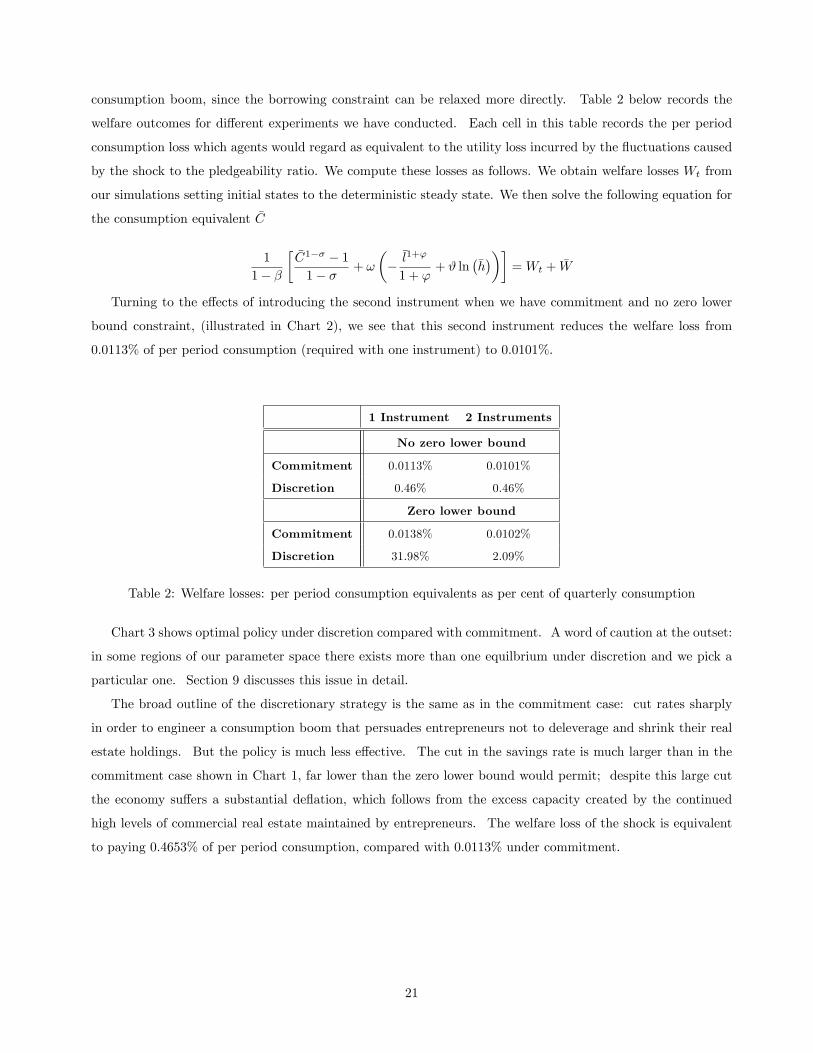
consumption boom, since the borrowing constraint can be relaxed more directly. Table 2 below records the
welfare outcomes for di¤erent experiments we have conducted. Each cell in this table records the per period
consumption loss which agents would regard as equivalent to the utility loss incurred by the �uctuations caused
by the shock to the pledgeability ratio. We compute these losses as follows. We obtain welfare losses Wt from
our simulations setting initial states to the deterministic steady state. We then solve the following equation for
the consumption equivalent �C
1
1� �
� �C1�� � 11� � + !
���l1+'
1 + '+ # ln
��h���
=Wt + �W
Turning to the e¤ects of introducing the second instrument when we have commitment and no zero lower
bound constraint, (illustrated in Chart 2), we see that this second instrument reduces the welfare loss from
0.0113% of per period consumption (required with one instrument) to 0.0101%.
1 Instrument 2 Instruments
No zero lower bound
Commitment 0.0113% 0.0101%
Discretion 0.46% 0.46%
Zero lower bound
Commitment 0.0138% 0.0102%
Discretion 31.98% 2.09%
Table 2: Welfare losses: per period consumption equivalents as per cent of quarterly consumption
Chart 3 shows optimal policy under discretion compared with commitment. A word of caution at the outset:
in some regions of our parameter space there exists more than one equilbrium under discretion and we pick a
particular one. Section 9 discusses this issue in detail.
The broad outline of the discretionary strategy is the same as in the commitment case: cut rates sharply
in order to engineer a consumption boom that persuades entrepreneurs not to deleverage and shrink their real
estate holdings. But the policy is much less e¤ective. The cut in the savings rate is much larger than in the
commitment case shown in Chart 1, far lower than the zero lower bound would permit; despite this large cut
the economy su¤ers a substantial de�ation, which follows from the excess capacity created by the continued
high levels of commercial real estate maintained by entrepreneurs. The welfare loss of the shock is equivalent
to paying 0.4653% of per period consumption, compared with 0.0113% under commitment.
21

5 10 15 200.3
0.2
0.1
0Saving Rate
5 10 15 200.3
0.2
0.1
0Borrowing Rate
5 10 15 200.040.02
00.020.04
HH. Consumption
5 10 15 20
0.1
0.2Ent. Consumption
5 10 15 20
0.05
0
0.05
CRE
5 10 15 200.4
0.2
0Leveraged returns
5 10 15 20
0.1
0.05
0Inflation
5 10 15 200.040.02
00.020.04
Output
discretion commitment
5 10 15 20
0.10
0.10.2
Int Goods Price
Chart 3: discretion vs commitment: 1 instrument, no zero lower bound
We next introduce the ZLB and compare commitment with discretion, in Chart 4. The outcome under
discretion is now much worse than that under commitment - the lines for commitment appear almost �at in
comparison with those under discretion. The welfare loss expressed as before rises from 0.4653% with no ZLB
to about 32% with the ZLB constraint. By contrast, under commitment, the ZLB is much less deleterious in
its e¤ects: the welfare loss of the shock rises from 0.0113% to 0.0138%. Note that under discretion we are
getting falls in output of more than 30%, and this far away from the steady state we have to take our �rst
order approximation with a pinch of salt. Chart 4 raises a few other questions. First, why is the welfare loss
imposed by the ZLB so much worse under discretion than commitment? Second, what is driving the result that
the outcomes are so bad under discretion? Third, why are interest rates actually rising under discretion with
the ZLB in place?
22

5 10 15 20
0
10
20x 103 Saving Rate
5 10 15 20
0
10
20x 103 Borrowing Rate
5 10 15 20
0.2
0.1
0HH. Consumption
5 10 15 204
2
0Ent. Consumption
5 10 15 206
4
2
0CRE
5 10 15 200.5
00.5
11.5
Leveraged returns
5 10 15 200.3
0.2
0.1
0Inflation
5 10 15 20
0.3
0.2
0.1
0Output
discretion commitment
5 10 15 20
1
0.5
0Int Goods Price
Chart 4: Discretion vs commitment at the ZLB with 1 instrument
One way to understand the di¤erence between the commitment and discretion is to recall the mechanism
by which policy operated in the absence of the zero lower bound. There, the reduction in permitted leverage
reduced the returns to �fully leveraged�commercial real estate investment, causing entrepreneurial investment
to drop in the absence of a countervailing policy strategy. That strategy was to cut the main policy rate when
the shock occurred, so as to induce a consumption boom that would raise entrepreneurs�pro�ts �and thereby
generate a positive income e¤ect boosting entrepreneurs� saving levels (mitigating the negative substitution
e¤ect associated with the initial reduction leveraged returns). With a zero lower bound this strategy becomes
impossible �a �paradox of stimulus�that has close parallels with the �paradox of toil�highlighted by Eggertson
2010. The reasoning is as follows. Suppose the policymaker were able to engineer a boom by reducing real
interest rates. This should increase entrepreneurial wealth, and thus raise their CRE holdings over the medium
term, as in Chart 3. But higher CRE implies that the economy would have a high level of productive capacity,
which in turn implies that intermediate goods prices would be relatively low over the medium term � since
commercial real estate, a productive input, would be relatively abundant. By pulling down �nal goods �rms�
marginal costs, this then implies that in�ation would be relatively muted in future periods. Note that in this
Calvo pricing setup in�ation can be expressed as a discounted sum of future intermediate goods prices.
But low future in�ation implies low initial in�ation expectations, which in turn implies a higher initial real
interest rate. This serves to undermine the initial attempt to cut real rates and stimulate consumption �and
if the zero lower bound features, it simply proves impossible to cut nominal rates by enough to ensure the
23
required initial consumption boom, given the subsequent de�ationary consequences. In short, stimulus implies
extra capacity, which induces disin�ationary (or de�ationary) pressure inconsistent with stimulus.
There is a slight complication that the above logic skirts. If a consumption boom were successfully engineered,
unit labour costs would presumably rise (re�ecting a reduced willingness on the part of workers to accept any
given wage, given that their marginal utility of consumption is lower in a boom). This is helpful to the
policymaker, putting upward pressure on in�ation expectations. For our �paradox of stimulus� to obtain we
need the disin�ationary consequences of increased CRE investment to exceed the in�ationary consequences of
a reduced willingness of household members to work.
So like Eggertson, we �nd that policymakers at the zero lower bound cannot be content with trying to
engineer higher potential output in future time periods, since this may actively preclude the intertemporal prices
required for demand to rise to meet this potential. Unlike Eggertson, we allow potential output to depend on
the (endogenous) level of commercial real estate investment in the economy, and hence to be in�uenced by
policy choices rather than being the product of consumers�exogenous desire to work. Thus our problem is more
a �paradox of stimulus�than a paradox of toil: if policymakers act under discretion, and so cannot commit to
higher in�ation at future horizons, they may �nd it impossible to inject stimulus via conventional monetary
policy instruments without destroying the very mechanism that boosts demand.
A prima facie reason for why the ZLB worsens outcomes so much more under discretion is that the �missing
stimulus� imposed by the ZLB is so much larger. This can be seen from Chart 3 where it is clear that the
optimal policy in the absence of the ZLB is for a larger cut on impact (thus a larger breach of the ZLB) than
under discretion. As to why outcomes are so bad, a key factor here is the interaction of the de�ation that
insu¢ ciently stabilising interest rate policy has with the borrowing constraint. Recall once more that this
constraint has bt = mtEt�t+1Qt
phe
t+1het . The failure to cut the savings rate induces a de�ation which exacerbates
the fall in borrowing bt necessitated by the fall in the pledgeability ratio mt, which in turn induces even greater
de�ationary pressure, and so on. Similarly, debt de�ation increases the real value of the debt burden and
reduces the borrowing capacity of entrepreneurs further. The impact of this debt de�ation can be seen by
simulating a version of the model in which private debt is indexed. Chart 5 does this. The impulses of all key
variables entering policymakers�loss function are substantially more benign when debt is indexed.
Finally, why are policy rates rising after the initial fall, especially when in�ation and output are so depressed?
The reason seems to be as follows. Partly because of the debt-de�ation mechanism described above, and its
anticipation, commercial real estate drops hugely on impact. Keeping interest rates low in the periods following
the shock would stimulate demand and push up on in�ation and output, but commercial real estate would move
back to steady state quickly following the large initial fall. Our quadratic loss function penalizes variations in
the growth rate of real estate and thus policymakers prefer to bring real estate back to target in a succession of
small steps following a large initial fall.
24
5 10 15 20
0
10
20x 103 Saving Rate
5 10 15 20
0
10
20x 103 Borrowing Rate
5 10 15 200.25
0.20.15
0.10.05
HH. Consumption
5 10 15 204
2
Ent. Consumption
5 10 15 206
4
2
CRE
5 10 15 200
1
Leveraged returns
5 10 15 200.3
0.2
0.1
0Inflation
5 10 15 20
0.3
0.2
0.1
Output
discretion nominal debt discretion indexed debt
5 10 15 20
1
0.5
0Int Goods Price
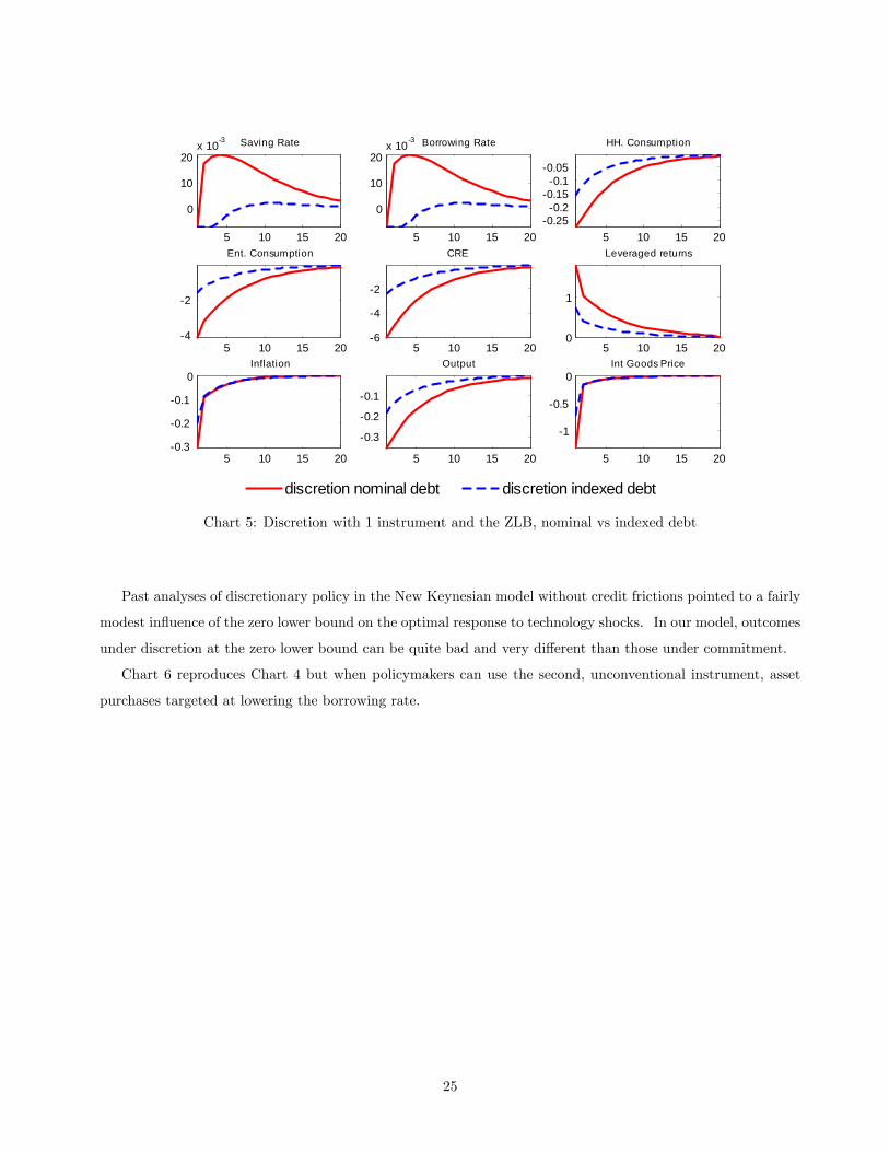
Chart 5: Discretion with 1 instrument and the ZLB, nominal vs indexed debt
Past analyses of discretionary policy in the New Keynesian model without credit frictions pointed to a fairly
modest in�uence of the zero lower bound on the optimal response to technology shocks. In our model, outcomes
under discretion at the zero lower bound can be quite bad and very di¤erent than those under commitment.
Chart 6 reproduces Chart 4 but when policymakers can use the second, unconventional instrument, asset
purchases targeted at lowering the borrowing rate.
25

5 10 15 20
5
0
5x 10 3 Saving Rate
5 10 15 200.80.60.40.2
0Borrow ing Rate
5 10 15 20
0.2
0.1
0HH. Consumption
5 10 15 202
1
0Ent. Consumption
5 10 15 20
0.05
0
0.05
CRE
5 10 15 200
2
4
Leveraged returns
5 10 15 200.3
0.2
0.1
0Inflation
5 10 15 20
0.2
0.1
0Output
discretion commitment
5 10 15 201
0.5
0Int Goods Price
Chart 6: optimal policy with 2 instruments and the ZLB
There are several points to note. Under commitment, the second instrument is used for stabililsation
purposes, but much less so than under discretion. This extra instrument improves the welfare loss associated
with the shock from 0.0138% to 0.0102% of quarterly consumption (Table 2). In the case of discretion there
is much greater exploitation of the second instrument (the borrowing rate falls dramatically). Outcomes for
in�ation and output are still of the same order of magnitude as with 1 instrument, but the stock of commercial
real estate falls by much less. This translates to a reduction in the welfare loss due to the shock of more than
a factor of 10, from about 32% to 2.1%of quarterly consumption. Once again, the precise numbers for the
discretion case are probably questionable, on account of the inaccuracy of our �rst order approximation so far
away from the steady state, but the qualitative point is clear. Having a second instrument is especially useful
when you can�t commit to managing expectations with the �rst.
The second point to take away from the experiment with 2 instruments and the ZLB (Chart 6) is that the
bene�ts of having the second instrument are magni�ed by the presence of the zero lower bound. This is true
for discretion and commitment. Looking back to Table 2: under commitment, the welfare gain from using
the second instrument (quanti�ed as before) amounts to a reduction in the compensating payments of 0.0012
percentage points without the ZLB, but with the ZLB this the second instrument reduces these payments by
26

0.0036 percentage points. For discretion, we record actually no bene�t of having the second instrument without
the ZLB, but a reduction in the payments required to compensate for the shock by a factor of more than 10
with the ZLB.
A �nal observation from our results concerns the bene�ts of commitment, or, as previous work termed it,
the size of the �stabilisation bias�. Using Table 2 we can deduce the following. With the ZLB, the bene�t of
commitment is greater when only 1 instrument is available than if 2 are. Without it, the bene�t of commitment
is not much a¤ected by the second instrument, but if anything the bene�t increases. The gain from commitment
is also much greater when the ZLB binds, regardless of whether the policymaker has access to 1 or 2 instruments.
9 Notes on multiplicity
For our baseline calibration, we �nd two Markov-stationary equilibria under discretion. The possibility that
there are multiple equilibria is a general property of rational expectations models with endogenous state variables
when policy is set optimally under discretion, as explained in Blake and Kirsanova (2010) or King and Wolman
(2004). In our model, the endogenous states are commercial real estate, entrepreneurial debt and the nominal
interest rate. Chart 7 below shows the dynamics for the two equilibria model under discretion when no zero
lower bound is imposed. Note that the second equilibrium displays a negative root in the decision rules giving
rise to oscillating dynamics.
5 10 15 200.30.20.1
0
Saving Rate
5 10 15 200.30.20.1
0
Borrowing Rate
5 10 15 200.05
0
0.05HH. Consumption
5 10 15 200.2
0
0.2Ent. Consumption
5 10 15 20
0.4
0.2
0
CRE
5 10 15 200.20.1
00.1
Leveraged returns
5 10 15 20
0.1
0.05
0Inflation
5 10 15 200.05
0
0.05
Output
equilibrium 1 equilibrium 2
5 10 15 20
0.10
0.10.2
Int Goods Price
Chart 7: Discretionary Policy: Dynamics under two di¤erent equilibria (no ZLB, one
instrument)
27

We neglect the equilibrium with oscillatory dynamics. We made this choice for 3 reasons. First, on
grounds of realism: if this economy were to be estimated, the oscillatory equilibrium would probably have
a lower likelihood. Second, on practical grounds: the oscillatory dynamics make it more cumbersome to
implement algorithm for solving for optimal policy in the presence of the zero bound. That process involves
guessing in which periods the lower bound is binding and when it is not, which is di¢ cult when interest rates
oscillates around zero. A third reason concerns what we �nd regarding the existence or otherwise of multiplicity
on a quick exploration of the parameter space de�ned by our model. The oscillatory equilibrium is the only one
that survives for values of our adjustment cost below the value we chose in our calibration. For values much
above our baseline value, only the non-oscillatory equilibrium survives. At intermediate values for adjustment
costs, both equilibria exist. If one assumes that the baseline calibration for adjustments is conservative and
adjustment costs could plausibly be higher, then focusing on the equilibrium that survives for higher adjustment
costs makes sense.
10 Conclusions
The contribution of this paper is to illustrate optimal monetary policy when there is access to a second uncon-
ventional instrument that a¤ects spreads on private borrowing rates, a zero lower bound constraint on moving
the conventional interest rate, when use of this second instrument has to be �nanced using distortionary tax-
ation, and when there is a shock to �nancial conditions that tightens borrowing constraints on �rms. Many
of these issues are dealt with in separate papers, but we bring them all together in one place, and by doing so
have a framework that can start to address what happened in the �nancial crisis.
The model we chose was a modi�cation of Iacoviello (2005) and Andres et al. (2009). The credit friction
in this model is that entrepreneurs,who are responsible for production, can only pledge a certain fraction of
their commercial real estate holdings as collateral against loans they need to �nance that production. We
modi�ed the model to incorporate costs of converting real estate from commercial to residential use and vice-
versa. We simulated the model in the face of a downward shock to this portion - the pledgeability ratio - which
reduces their borrowing capability. The unconventional policy instrument works directly against this friction.
This instrument involves central bank purchases of claims issued by banks on the income streams �owing from
loans made by them to entrepreneurs: essentially central bank purchases of securitised loans to �rms. These
purchases drive prices above (yields below) what would otherwise have prevailed.
Optimal monetary policy with one instrument aims at trying to generate an income e¤ect for entrepreneurs
to o¤set the substitution e¤ect of the tightening in the borrowing constraint encouraging them to deleverage
and scale back on their commercial real estate holdings. Using the second instrument rather unsurprisingly
improves matters, because this second instrument helps relax the borrowing constraint directly. The zero lower
bound constraint obviously has a deleterious e¤ect on welfare, relative to the case where it is absent, and a
disastrous e¤ect when policy is set with discretion, using 1 instrument only. The potential for such large e¤ects
28

was not evident from previous studies which did not consider the interaction of the zero bound with credit
frictions. The bene�t of the second instrument is magni�ed by the presence of the zero lower bound (an extra
instrument is even more helpful when you can�t move the �rst) or when commitment is not possible. Our
experiments allow us to investigate the determinants of the welfare cost of not being able to commit. These
are increased by the presence of the zero lower bound: this eliminates the possibility of substituting cutting
the short rate for managing expected future short rates. And these costs of discretion are reduced by having a
second instrument, with our without the zero lower bound. In part, our unconventional tool makes up for not
being able to manage expected future short rates.
References
K. Adam and R. Billi. Discretionary monetary policy and the zero lower bound on nominal interest rates.
Journal of Monetary Economics, 54(3):728�752, 2007.
J. Andres, O. Arce, and C. Thomas. Banking competition, collateral constraints and optimal monetary policy.
Bank of Spain working paper 1001, 2009.
A. Blake and T. Kirsanova. Discretionary policy and multiple equilibria in lq re models. University of Exeter,
2010.
Vasco Curdia and Michael Woodford. The central bank balance sheet as an instrument of monetary policy.
NBER working paper no 16208, 2010.
G.B. Eggertson and M. Woodford. The zero bound on interest rates and optimal monetary policy. Brookings
Papers on Economic Activity, 34:139�235, 2003.
G.B. Eggertson and M. Woodford. Optimal monetary and �scal policy in a liquidity trap. NBER working
papers no 10840, 2004.
G.B. Eggertson, M. DelNegro, A. Ferrero, and N. Kiyotaki. The great escape? a quantitative evaluation of the
fed�s non-standard policies. Federal Reserve Bank of New York, 2009.
Joseph Gagnon, Matthew Raskin, Jile Remache, and Brian Sack. Large-scale asset purchases by the federal
reserve: Did they work? Federal Reserve Bank of New York Sta¤ Report no 441, March 2010.
M. Gertler and P. Karadi. A model of unconventional monetary policy. New York University, 2009.
Robin Greenwood and Dimitri Vayanos. Price pressure in the government bond market. American Economic
Review, pages 585�590, 2010.
R. Harrison. Asset purchase policy at the e¤ective lower bound for interest rates. Bank of England, 2010.
29

M. Iacoviello. House prices, borrowing constraints, and monetary policy in the business cycle. American
Economic Review, 95(3):739�764, 2005.
Michael Joyce, Ana Lasosa, Ibrahim Stevens, and Matthew Tong. The �nancial market impact of quantitative
easing. Bank of England working paper no 393, 2010.
Taehun Jung, Yuki Teranishi, and Tsutomu Watanabe. Optimal monetary policy at the zero-interest-rate
bound. Journal of Money, Credit and Banking, 37(5):813�35, October 2005.
Nobuhiro Kiyotaki and John Moore. Credit cycles. Journal of Political Economy, 105(2):211�248, 1997.
N. Kiyotaki and J. Moore. Liquidity, monetary policy and business cycles. Princeton University, 2008.
Anton Nakov. Optimal and simple monetary policy rules with zero �oor on the nominal interest rate. Interna-
tional Journal of Central Banking, 4(2):73�127, June 2008.
Neil Wallace. A modigliani-miller theorem for open-market operations. American Economic Review, 71(2):267�
74, 1981.
11 Appendix: deriving the policymaker�s loss function
This derivation follows closely Andres et al (2010), which applies the logic set out in Woodford (2003) and
elsewhere to derive an approximation to a function that maximises the welfare of the agents inhabiting our
model economy. The loss function is derived from a second-order log approximation to the policymaker�s
objective function in the region of a zero-in�ation, optimal steady state.6 We �rst present the derivation of that
approximation, and then turn to explain the derivation of the tax processes required to ensure that the steady
state is distortion free.
First, we take a second-order log approximation to Wt directly:
Wt = Et
1Xs=0
�sf!c1��ss
�bct+s + 12(1� �)bc2t+s�
+(1� !) c1��ss
�bcet+s + 12 (1� �) �bcet+s�2�
�!l1+'ss
�blst+s + 12 (1 + ')�blst+s�2�+ !#bht+sg+O3. (57)
Next, we do likewise to the goods market equilibrium condition, making use of the fact that small deviations
in prices do not a¤ect the price dispersion index in a zero-in�ation steady state, so linear deviations in the log
of this index are already re�ecting �second-order��uctuations:6Approximating the model with log deviations makes the algebra more tractable, but requires us to neglect cases where � < 1
if we are to use standard linear-quadratic techniques subsequently, since in this event consumption utility is a convex function ofits log deviation from steady state, and the objective weight matrix may no longer be positive-semi-de�nite.
30

(1� !) yss�byt + 1
2by2t � b�t� = !css
�bct + 12bc2t�
+(1� !) css�bcet + 12 (bcet )2
�+ " (hess)
2�bhet � bhet�1�2 +O3, (58)
where we have also used the fact that ct = cet must hold in any optimal steady state. Squaring both sides of
this last equation and rearranging then gives:
by2t = � !
(1� !)cssyss
�2 bc2t + � cssyss�2(bcet )2 + 2 !
(1� !)
�cssyss
�2 bctbcet +O3, (59)
which, together with the condition cssyss
= (1� !) (which follows from goods market clearing when ct = cet )
and some manipulation, gives us:
byt = !bct + (1� !)bcet + b�t + 12! (1� !) (bct � bcet )2 + " (hess)2
(1� !) yss
�bhet � bhet�1�2 +O3. (60)
The production function is log-linear, and can be used to replace terms in labour supply; we have:
byt = bat + (1� v)blst + vbhet�1. (61)
Collecting these expressions together, the objective can be written as:
Wt = Et
1Xs=0
�sfc1��ss [byt+s � b�t+s � 12! (1� !)
�bct+s � bcet+s�2� " (hess)
2
(1� !) yss
�bhet+s � bhet+s�1�� 12 (� � 1)�!bc2t+s + (1� !) �bcet+s�2�� (1� v)
byt+s � at+s � vbhet+s�1(1� v) +
1
2
(1 + ')
(1� v)2�byt+s � bat+s � vbhet+s�1�2
!]
+!#bht+sg+O3. (62)
(This uses the fact that ! (lsss)1+'
= (1� v) c1��ss follows jointly from steady-state equilibrium in the goods
and labour markets �assuming that the distortionary impact of �nal goods �rms�market power has been o¤set,
as outlined below.)
Next we exploit a second-order approximation to the real-estate market clearing condition, giving:
!hss
�bht + 12bh2t�+ (1� !)hess�bhet + 12 �bhet�2
�= 0. (63)
An optimal steady state must involve the marginal (social) value product of a unit of real estate used
31

for commercial purposes being equal to the marginal (social) value of the residential services it could deliver.
Together with goods market clearing, that implies:
#h�1ss =�v
(1� !)c1��ss
hess. (64)
Inserting this in the previous equation and simplifying:
!#bht + �vc1��ssbhet = �12
�!#bh2t + �vc1��ss
�bhet�2� . (65)
Some protracted but ultimately straightforward algebra (see, for instance, Woodford, 2003) allows the price
dispersion terms near a zero-in�ation steady state to be expressed as squared deviations of the in�ation rate:
1Xs=0
�s b�t+s = �
1� ��b�t�1 + 1
2
"�
(1� �) (1� ��)
1Xs=0
�sb�2t+s. (66)
So that we �nally have:
Wt = �12c1��ss Et
1Xs=0
�sf! (1� !)�bct+s � bcet+s�2
+(� � 1)�!bc2t+s + (1� !) �bcet+s�2�+ 2 " (hess)
2
(1� !) yss
�bhet+s � bhet+s�1�2+1 + '
1� v
�byt+s � byflt+s�2 + "�
(1� �) (1� ��)b�2t+s + �v!#+ �vc1��ss
!#
�bhet+s�2g+t:i:p:+O3, (67)
where the terms in at+s and the initial states b�t�1 and bhet�1 are noted to be independent of policy.
12 Appendix: steady-state taxes
A �simple�linear-quadratic approach to the optimal policy problem �in which a second-order approximation
to the policymaker�s objective criterion is maximised subject to �rst-order approximations to the economy�s
equilibrium conditions �will in general only be appropriate to �nding the best path in the neighbourhood of a
steady state that is itself optimal from the policymaker�s perspective. This steady-state optimality implies the
�rst-order e¤ects of �uctuations on the value of the objective function are zero (given the equilibrium restrictions
constraining their impact) �a fact that can be used to eliminate linear terms from the second-order expansion
of the welfare criterion, as we do above. Given a purely quadratic approximation to the objective, the second-
order e¤ects of �uctuations on the policymaker�s constraints can be neglected �since the impact on welfare of
�rst-order relaxations of these constraints is already of second order at best.7 To ensure this approximation is7Benigno and Woodford (2008) present general methods for obtaining a linear-quadratic formulation of the optimal policy
problem without introducing steady-state taxes. But their method relies on the �timeless perspective�criterion for ranking stationary
32
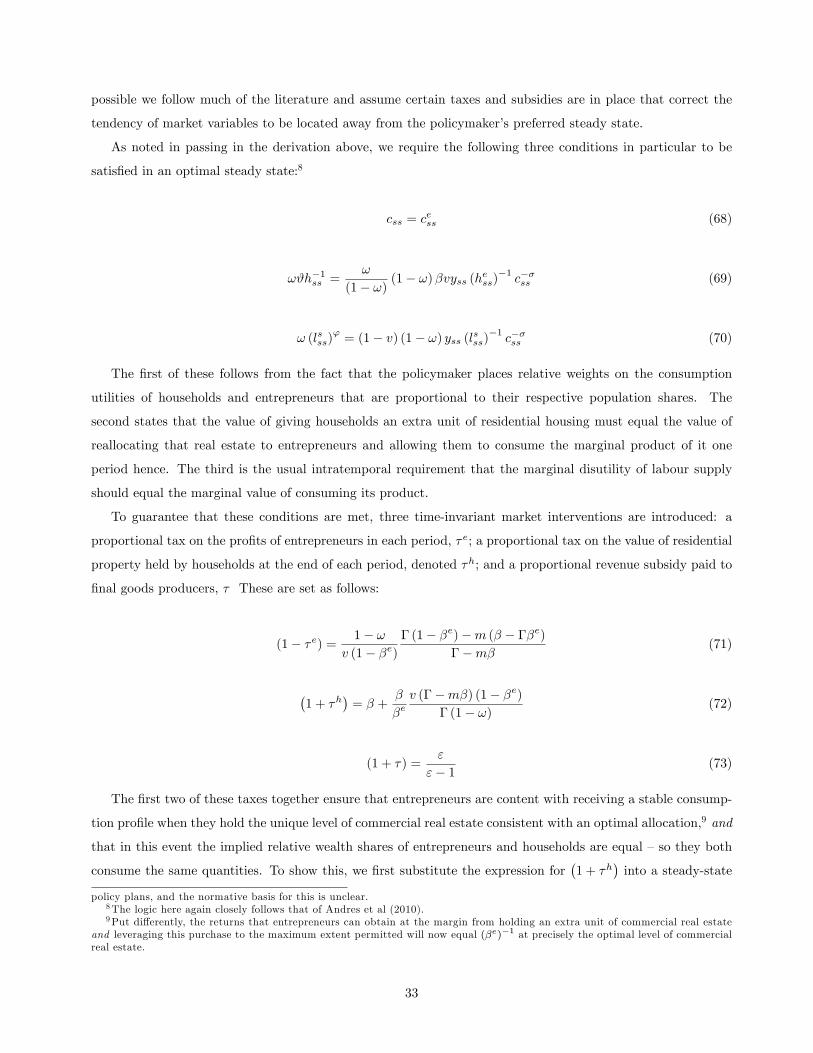
possible we follow much of the literature and assume certain taxes and subsidies are in place that correct the
tendency of market variables to be located away from the policymaker�s preferred steady state.
As noted in passing in the derivation above, we require the following three conditions in particular to be
satis�ed in an optimal steady state:8
css = cess (68)
!#h�1ss =!
(1� !) (1� !)�vyss (hess)
�1c��ss (69)
! (lsss)'= (1� v) (1� !) yss (lsss)
�1c��ss (70)
The �rst of these follows from the fact that the policymaker places relative weights on the consumption
utilities of households and entrepreneurs that are proportional to their respective population shares. The
second states that the value of giving households an extra unit of residential housing must equal the value of
reallocating that real estate to entrepreneurs and allowing them to consume the marginal product of it one
period hence. The third is the usual intratemporal requirement that the marginal disutility of labour supply
should equal the marginal value of consuming its product.
To guarantee that these conditions are met, three time-invariant market interventions are introduced: a
proportional tax on the pro�ts of entrepreneurs in each period, �e; a proportional tax on the value of residential
property held by households at the end of each period, denoted �h; and a proportional revenue subsidy paid to
�nal goods producers, � These are set as follows:
(1� �e) = 1� !v (1� �e)
� (1� �e)�m (� � ��e)��m� (71)
�1 + �h
�= � +
�
�ev (��m�) (1� �e)
� (1� !) (72)
(1 + �) ="
"� 1 (73)
The �rst two of these taxes together ensure that entrepreneurs are content with receiving a stable consump-
tion pro�le when they hold the unique level of commercial real estate consistent with an optimal allocation,9 and
that in this event the implied relative wealth shares of entrepreneurs and households are equal �so they both
consume the same quantities. To show this, we �rst substitute the expression for�1 + �h
�into a steady-state
policy plans, and the normative basis for this is unclear.8The logic here again closely follows that of Andres et al (2010).9Put di¤erently, the returns that entrepreneurs can obtain at the margin from holding an extra unit of commercial real estate
and leveraging this purchase to the maximum extent permitted will now equal (�e)�1 at precisely the optimal level of commercialreal estate.
33

version of the household optimality condition for residential property holdings, obtaining:
c��ss phss
�
�ev (��m�) (1� �e)
� (1� !) = #h�1ss . (74)
Similarly, inserting the expression for (1� �e) into a steady-state version of the entrepreneur�s Euler condi-
tion and simplifying gives:
phss = �e(1� !) �
v (��m�) (1� �e)vysshess
. (75)
Using this equation in the previous con�rms that the allocation of real estate is optimal. To show that entre-
preneurial and household consumption levels are equal, we use the entrepreneurial budget constraint together
with the expression for (1� �e) and the solution for phss just derived, simplifying down to obtain:
cess = (1� !) yss. (76)
Steady-state goods market clearing gives us !css + (1� !) cess = (1� !) yss, and equal consumption imme-
diately follows.
Finally, the �rst-order condition for optimal price-setting on the part of �nal goods �rms in steady state
gives:
(1 + �) ="
"� 1pIss. (77)
Intermediate goods �rms set the (real) marginal revenue product of hiring an additional worker equal to the
real wage:
pIss (1� v)yssldss
= wss. (78)
Workers allow their marginal rate of substitution to equal the same:
(lsss)'c�ss = wss. (79)
Labour market clearing (!lsss = (1� !) ldss), together with the value pIss = 1 implied by � , then con�rms the
�nal optimality condition.
13 Appendix: a new algorithm for solving for optimal monetary
policy under discretion with inequality constraints
The economy is described by a set of linear rational-expectations equations, stacked in matrix form to give:
34

A0yt = A1yt�1 +A2Etyt+1 +A3xt +A4xt�1 +A5vt, (80)
where yt is a vector of endogenous variables, xt a vector of controls and vt a vector of mean-zero, iid
disturbances. Additionally, a set of inequality restrictions constrain the behaviour of the control variables:
Sxt � s, (81)
where s is a vector of constants and S a coe¢ cient matrix. The policymaker sets these controls in order to
minimise the discounted sum of loss Lt:
Lt = Et
1Xs=0
�sy0t+sWyt+s, (82)
where W is a symmetric, positive-semi-de�nite weighting matrix and � 2 [0; 1) the rate of pure time
preference.10
The policymaker at time t is unable to commit to a policy strategy at later dates, and must therefore take
future policy responses to the state of the economy as given �e¤ectively playing the role of Stackelberg leader
in a non-cooperative game with its own future incarnations. We initially assume that in the equilibrium under
study the policymaker at time t+ 1 behaves in a way that ensures the following state-contingent evolution for
the endogenous variables:
yt+1 = H1;t+1yt +H2;t+1xt +H3;t+1vt+1 +H4;t+1, (83)
where the transition matrices are indexed by the time period to which they apply. H4;t+1 is a vector of
constants that will enter into equilibrium behaviour in the event that certain policy variables are constrained
to equal non-zero scalar values.
This implies that the policymaker acting at time t faces the following consolidated constraint, alongside the
inequality restrictions:
(A0 �A2H1;t+1) yt = A1yt�1 + (A3 +A2H2;t+1)xt +A4xt�1 +A5vt +A2H4;t+1. (84)
We require for what follows that (A0 �A2H1;t+1) is invertible. The piecewise approach to solving the
model under inequality constraints assumes perfect foresight in the aftermath of a shock, allowing one to
specify the precise timing of transition from one �regime�to another along the stabilisation path (where each
regime is characterised by a distinct subset of the inequality constraints binding). This is an extremely useful
simpli�cation for our purposes, as it allows us to �nd a discretionary equilibrium by working backwards ��rst
solving for a stationary Markov equilibrium in the regime consistent with the control variables being close to
10 It would be straightforward to generalise to cases in which the policymaker also faces loss directly from deviations in the controlvariables xt, and indeed to cases in which expected future values of the controls feature in the model�s structural equations.
35

steady state, then �nding the optimal response to this future behaviour in earlier periods, that are subject to
di¤erent binding policy constraints. To this end we set up a value function problem with the advantage that it
can be solved iteratively for a stationary solution in the terminal regime whilst still characterising the optimal
policy problem along the prior, non-stationary path. Given the linear-quadratic nature of the problem, it makes
sense to conjecture that the value function in the arbitrary time period t+ 1 satis�es:
Vt+1 (yt; xt) = y0tVyyt+1yt + 2y
0tV
yxt+1xt + x
0tV
xxt+1xt + 2y
0tV
yct+1 + 2x
0tV
xct+1 +�t+1, (85)
using superscript notation in the obvious way (c indicates constant terms), and collecting in �t+1 the sum
of all terms that involve the shock vector, together with a constant (these are not relevant to the analysis that
follows). The linear terms in the lagged endogenous and control variables will be non-zero in the event that
policy is constrained by a non-zero scalar. We assume that the combined value matrix conformable with the
vector zt � [y0t; x0t]0, obtained by collecting the relevant sub-components above, is positive semi-de�nite. Given
this, by the de�nition of the value function the policymaker at time t faces the following problem (written in
Lagrangian form):
minxt;yt
max�t;�t=0
fy0tWyt + �Vt+1 (yt; xt)� 2�0t[(A0 �A2H1;t+1) yt
�A1yt�1 � (A3 +A2H2;t+1)xt �A4xt�1 �A5vt �A2H4;t+1]
�2�0t (Sxt � s)g. (86)
Reasoning in the usual way, four necessary conditions for an optimum are:
�W + �V yyt+1
�yt + �V
yxt+1xt + �V
yct+1 �
�A00 �H 0
1;t+1A02
��t = 0, (87)
��V yxt+1
�0yt + �V
xxt+1xt + �V
xct+1 +
�A03 +H
02;t+1A
02
��t � S0�t = 0, (88)
(A0 �A2H1;t+1) yt �A1yt�1 � (A3 +A2H2;t+1)xt �A4xt�1 �A5vt �A2H4;t+1 = 0, (89)
�0t (Sxt � s) = 0. (90)
Manipulating the �rst of these:
�t =�A00 �H 0
1;t+1A02
��1 ��W + �V yyt+1
�yt + �V
yxt+1xt + �V
yct+1
�, (91)
which implies:
36

��V yxt+1
�0yt + �V
xxt+1xt + �V
xct+1
+�A03 +H
02;t+1A
02
� �A00 �H 0
1;t+1A02
��1 ��W + �V yyt+1
�yt + �V
yxt+1xt + �V
yct+1
�= S0�t. (92)
The third condition solves for yt:
yt = (A0 �A2H1;t+1)�1[A1yt�1 + (A3 +A2H2;t+1)xt +A4xt�1 +A5vt +A2H4;t+1] . (93)
Combining the previous two equations, we have a relationship describing the optimal values for the t-dated
controls, of the form:
�1xt +�2yt�1 +�3xt�1 +�4vt +�5 � S0�t = 0, (94)
where:
�1 = [��V yxt+1
�0+�A03 +H
02;t+1A
02
� �A00 �H 0
1;t+1A02
��1 �W + �V yyt+1
�] (95)
� (A0 �A2H1;t+1)�1(A3 +A2H2;t+1) + �V
xxt+1 +
�A03 +H
02;t+1A
02
� �A00 �H 0
1;t+1A02
��1�V yxt+1,
�2 =h��V yxt+1
�0+�A03 +H
02;t+1A
02
� �A00 �H 0
1;t+1A02
��1 �W + �V yyt+1
�i(A0 �A2H1;t+1)
�1A1, (96)
�3 =h��V yxt+1
�0+�A03 +H
02;t+1A
02
� �A00 �H 0
1;t+1A02
��1 �W + �V yyt+1
�i(A0 �A2H1;t+1)
�1A6, (97)
�4 =h��V yxt+1
�0+�A03 +H
02;t+1A
02
� �A00 �H 0
1;t+1A02
��1 �W + �V yyt+1
�i(A0 �A2H1;t+1)
�1A5, (98)
�5 = [��V yxt+1
�0+�A03 +H
02;t+1A
02
� �A00 �H 0
1;t+1A02
��1 �W + �V yyt+1
�] (99)
� (A0 �A2H1;t+1)�1A2H4;t+1 + �V
xct+1 +
�A03 +H
02;t+1A
02
� �A00 �H 0
1;t+1A02
��1�V yct+1.
Provided �1 is non-singular, this relationship will allow us to tie down the value of the controls at time
t in precisely as many dimensions as are left free by the complementary slackness condition on the inequality
constraints (where an inequality constraint binds, the above condition tells us the value of the multiplier on it).
Solving for xt is therefore a matter of combining the inequality constraints with the previous expression in a
37

way that will always permit a solution for xt. Stacking the two, we have:24 I � Jk JkS
�S0Jk �1
3524 �t
xt
35 =24 0 0
��2 ��3
3524 yt�1
xt�1
35+24 0 JkS
��4 ��5
3524 vt
1
35 , (100)
where Jk is an indicator matrix that has unit entries on the diagonal at positions corresponding to non-zero
elements of �t, and zeros elsewhere. The coe¢ cient matrix on the left-hand side here is then invertible by
construction (again, provided �1 is non-singular). Inverting it allows us to extract a solution for xt in the form:
xt = F1;tyt�1 + F2;txt�1 + F3;tvt + F4;t, (101)
where the coe¢ cient matrices here are read o¤ from the relevant blocks in the matrices
24 I � Jk JkS
�S0Jk �1
35�1 24 0 0
��2 ��3
35 and24 I � Jk JkS
�S0Jk �1
35�1 24 0 JkS
��4 ��5
35.
Using this to replace the contemporaneous controls in the earlier solution for yt, we have an evolution
equation for the endogenous variables in the desired form:
yt = H1;tyt�1 +H2;txt�1 +H3;tvt +H4;t, (102)
where:
H1;t = (A0 �A2H1;t+1)�1[A1 + (A3 +A2H2;t+1)F1;t] , (103)
H2;t = (A0 �A2H1;t+1)�1[A4 + (A3 +A2H2;t+1)F2;t] , (104)
H3;t = (A0 �A2H1;t+1)�1[A5 + (A3 +A2H2;t+1)F3;t] , (105)
H4;t = (A0 �A2H1;t+1)�1[A2H4;t+1 + (A3 +A2H2;t+1)F4;t] . (106)
This therefore gives us an updating procedure for the policymaker�s optimal law of motion for the endogenous
variables, given the behaviour of future policymakers. Using these solutions for xt and yt, we are able to
substitute in to the t-dated objective function directly, and express the minimum value of the policymaker�s loss
function in terms of yt�1, xt�1, vt and a constant. Doing so yields the following solutions for the value matrices
speci�ed above:
38

V yyt = H 01;t
�W + �V yyt+1
�H1;t + �H
01;tV
yxt+1F1;t + �F
01;t
�V yxt+1
�0H1;t + �F
01;tV
xxt+1F1;t, (107)
V yxt = H 01;t
�W + �V yyt+1
�F2;t + �H
01;tV
yxt+1F2;t + �F
01;t
�V yxt+1
�0H2;t + �F
01;tV
xxt+1F2;t, (108)
V xxt = H 02;t
�W + �V yyt+1
�H2;t + �H
02;tV
yxt+1F2;t + �F
02;t
�V yxt+1
�0H2;t + �F
02;tV
xxt+1F2;t, (109)
V yct = H 01;t
�W + �V yyt+1
�H4;t + �H
01;tV
yxt+1F4;t + �F
01;t
�V yxt+1
�0H4;t
+�F 01;tVxxt+1F4;t + �H
01;tV
yct+1 + �F
01;tV
xct+1, (110)
V xct = H 02;t
�W + �V yyt+1
�H4;t + �H
02;tV
yxt+1F4;t + �F
02;t
�V yxt+1
�0H4;t
+�F 02;tVxxt+1F4;t + �H
02;tV
yct+1 + �F
02;tV
xct+1. (111)
Given a particular �steady state�regime �characterised by the relevant indicator matrix Jk (denoting the
inequality constraints that bind in the region of steady state) � we can use the results above to obtain a
stationary Markov equilibrium, which is assumed to obtain in perpetuity in our perfect foresight equilibrium
once the impact of initial shocks has faded su¢ ciently. To be clear, the algorithm for �nding this equilibrium
is as follows:
1. Initialise values for the H and V matrices that are assumed to apply at some terminal date T . In appli-
cations we have found that null matrices usually su¢ ce, though if multiple stationary Markov equilibria
exist, di¤erent initialisations for the terminal value matrices can be used to �nd these.11
2. Iterate �backwards through time�, solving for the H and V matrices at each horizon given their next-period
value, using the method outlined above. Continue until all matrices have converged (with H1;t = H1;t+1,
V yyt = V yyt+1 and so on).
The �terminal�stationary equilibrium found, we know that the policymaker choosing in the last period of the
regime that is immediately prior to the terminal one faces a next-period value function and transition equation
consistent with that terminal equilibrium, but must optimise with a di¤erent sub-set of the inequality constraints
binding (that is, applying a di¤erent value of the indicator matrix Jk). Optimal dynamics in that period will
thus satisfy H and F matrices that are obtained from a single application of the solution procedure above,
11One might conjecture that a set of null terminal value matrices should always deliver convergence on the stationary equilibriumthat delivers lowest loss, though this may not be true for all initialisations of the H matrices.
39
inputting next-period value and transition matrices associated with the terminal equilibrium but constraints
consistent with the prior regime. This in turn implies a distinct set of value matrices associated with that
particular time period. One can work backwards in precisely the same way for as many periods (and through
as many regime shifts) as required, retaining the value and transition matrices (both H and F ) at each horizon,
so as to be able to chart the non-stationary evolution of the variables of interest proceeding from any initial
shocks.
The precise sequencing of regimes unfortunately requires some guesswork. In general a solution must be
characterised by the inequality constraints being satis�ed, and the multipliers associated with these inequality
constraints being non-negative, at all horizons. But these conditions can only be checked after solving the model
for a hypothetical sequencing: if satis�ed, the associated dynamics constitute a discretionary equilibrium; if not,
one must start again with a new conjecture for the timing of the di¤erent regimes.
40