Optimal Control with State Observer of - serialsjournals.com · Optimal Control with State Observer of ... in three-phase stator winding (a1, b1, c1, a2, b2, c2) of a two-phase model

I J C T A, 9(2-A), 2016, pp. 369-384

© International Science Press

* U.R Automation & Robotics Marine (ARM), Naval Academy, Emails: [email protected], [email protected],

[email protected]

Optimal Control with State Observer ofShip Electric Propulsion System UsingDouble Star Synchronous MachineHabib Dallagi*, Salmen Jaouidi* and Samir Nejim*

ABSTRACT

In this paper we are interested on themodelling, optimal control and numerical simulation of the ship electric

propulsion system provided by a double star synchronous machine. The in-depth analysis of the operation of the

propulsion system of the vessel allowed us to model elements of the propulsion system. Thus, a non-linear global

model was obtained describing the operation of the entire propulsion system. The global model of the electric

propulsion system of describing the dynamic behavior of the ship is nonlinear, multivariable and strongly coupled,

which makes its control difficult. The nonlinear model is linearized about the nominal operating point on which an

optimal control using a ship speed state observer is applied. The performances and the effectiveness of the studied

approach applied to a ship electric propulsion is highlighted through numerical simulation, using Matlab/Simulink,

to ensure perfect tracking of ship speed.

Keywords: Optimal control, Sate observer, Double star Synchronous motor, Ship electrical propulsion system.

1. INTRODUCTION

Today one notes a tendency toward the use of electrical power for ship propulsion which is made possible thanks

to the improvement of the power electronics components. The advantage of the electric propulsion ship is to

globalize all needs in energy, and with the same generators, to provide the necessary electrical power to the

propulsion and to the local electric network [4], [10]. Some recent control methods are discussed in [15-20].

The major decision criteria for the adoption of electric propulsion vary from one ship type to another,

acoustic discretion for submarines, research vessels and military ship, low noise and vibration for the ship

cruise, perfect torque control at all speeds for an icebreaker, precision and flexibility for maneuverfor

dynamic positioning ships, ferries or fishing vessels, space saving on tankers, to increase cargo or decrease

the length of the vessels. To these criteria are added the advantages common to all types of ship, such as:

reduced maintenance, increased operational safety, reduced pollution.

The multiphase machines are the subject of growing interest, especially the double synchronous motor

star ‘DSMS’ for different reason, such as:

- As the multiphase machine contains several phases, this for a given power, the electric currents are

reduced by phase and that power is distributed over the number of phases.

- Improved reliability by providing the ability to function properly degraded systems.

Generally the electrical equipment comprises two sets: Power & Propulsion:

- The power plant comprises generators driven by diesel engines. It supplies energy for all the

distributors on the ship and in particular for propulsion equipment.

370 Habib Dallagi, Salmen Jaouidi and Samir Nejim

- The propulsion equipment comprises electric motors, controlled continuously by frequency

converters for varying the speed of the propellers from 0 to 100% in both directions of rotation.

Unlike diesel engines, the electric motors powered by the frequency converters are able to provide

maximum torque at all times, even at very low speeds and in both directions of rotation. They

therefore used the propeller with fixed blades whose braking ability of the ship is excellent when

the rate is controlled by an electric motor. The torque provided by the electric motor is used to drive

the propeller back whatever the speed of the ship. This paper deals mainly electric propulsion of a

vessel equipped with a double Star synchronous motor. Modeling techniques for vessels electrically

driven such that the electric drive motor, the propeller and movement of the ship, having a non-

linear behaviour, have been developed. A simulation of the electric propulsion system of a vessel

with control loop has been performed using the Matlab/Simulink software.

The first section is consecrated to the ship electric propulsion. The second section is devoted to the

modeling of ship electric propulsion system. The resulting nonlinear model is linearized around nominal

operating point is treated to third section. The fourth section focuses to techniques of optimal control and

its main criteria. The observer construction is studied in the fifth section and in the last section numerical

simulations using the Matlab/Simulink software are reported to highlight the efficiency of the proposed

control scheme.

2. SHIP ELECTRIC PROPULSION SYSTEM MODEL

2.1. Description of ship propulsion system

The electric motor of propulsion is entirely integrated in a directional nacelle fixed under the hull outside

the ship Fig.1. The motor is coupled mechanically with a fixed blade propeller shaft. The electric machine,

which equips the ships, must be [4]:

- Compact, light and reliable.

- Robust to the marine environment (vibration, moisture, saline environment, temperature variation).

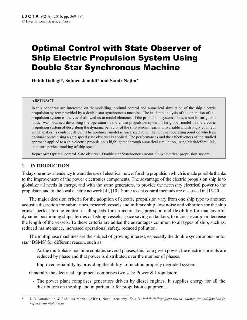
- Discrete with low noises and vibrations. In addition the forces applied to the ship are:

T: thrust developed by propeller,

R: the hull resistance applied by the sea opposing the ship movement

Text

: applied strength by the outside environment on the ship, induced by the wind and the waves

Fig.1.

Figure 1: The force representation applied to a ship

Optimal Control with State Observer of Ship Electric Propulsion System... 371

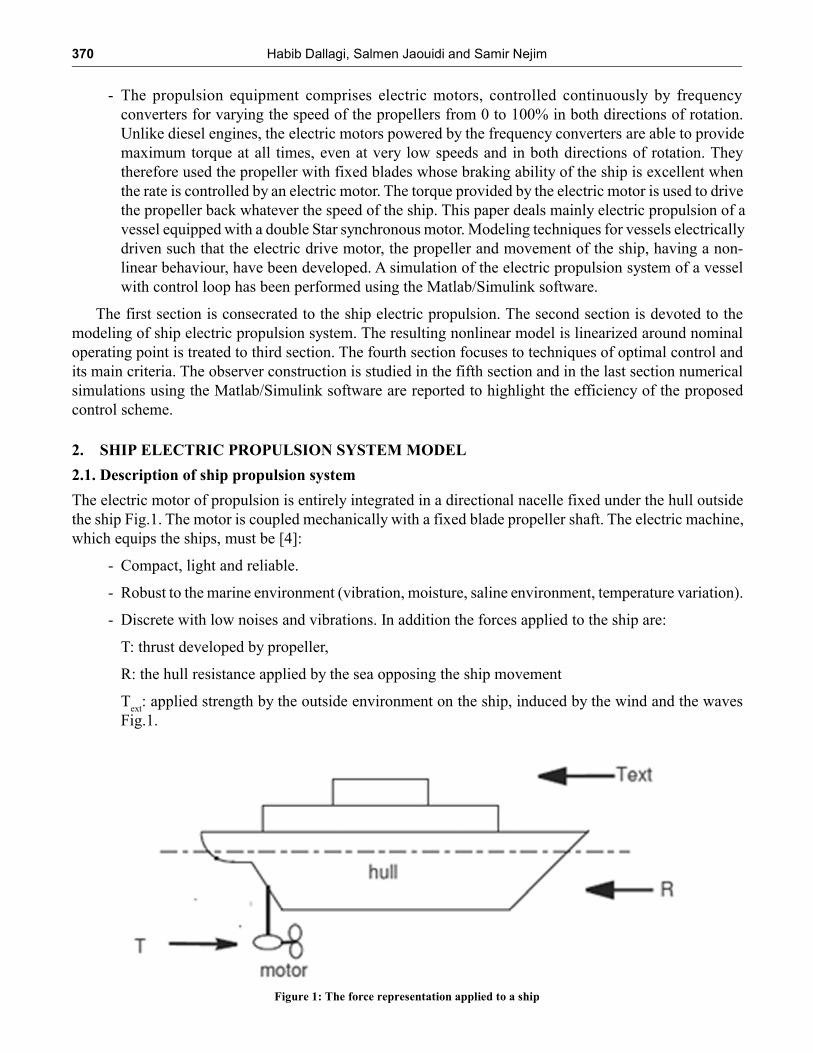
2.2. Double star synchronous motor model

The propulsion of the ship is provided by a motor MSDE. The model of the machine in the natural base is

significantly complicated because of the dependence of the inductance to the rotor position Fig. 1. To

overcome to this complexity, that the Park transformation consists in converting the model of the machine

in three-phase stator winding (a1, b1, c1, a2, b2, c2) of a two-phase model axis (d, q is used ) [1, 2, 10]. This

transformation is represented by the Fig. 2. The double star synchronous motor built with two symmetrical

tree phase armature winding systems, electrically shifted by 30° and its rotor is excited by current source.

Figure 2: MSDE Machine and Park MSDE representation, with = 30°

The voltage equations of the double star synchronous motor are written as follows [2], [11], [12], [13].

1 1 1 1

2 2 2 2

1 1 1 1

2 2 2 2

d S d d r q

d S d d r q

q S q q r d

q S q q r d

f

f f f

dV R I

dt

dV R I

dt

dV R I

dt

dV R I

dt

dV R I

dt

(1)

2.2.1. Magnetic Equations

1 1 2

2 2 1

1 1 2

2 2 1

1 2

d d d d d fd f

d d d d d fd f

q q q q q

q q q q q

f f f fd d d

L I M I M I

L I M I M I

L I M I

L I M I

L I M I I

(2)


The different currents 1 2 1 2, , , ,

d d q q fI I I I I are calculated based on flux

1 2 1 2, , , ,

d d q q f

From the eq. (2) of flux we obtain the following expressions:

1 21 2 2

1 22 2 2

1 2

1 2 2

1 2

2 2 2

fdd d d dd f

d d d d

fdd d d dd f

d d d d

q q q q

q

q q

q q q q

q

q q

ML MI I

L M L M

MM LI I

M L L M

L MI

L M

M LI

M L

(3)

2.2.2. Electromagnetic torque

The electromagnetic torque is produced by the interaction between the poles formed by magnets to the

rotor and the poles caused by magneto-motive F.M.M force in the gap generated by the stator currents. It is

expressed by: 1 2 em em emC C C

With: 1 1 1 1 1 em d q q dC p I I and 2 2 2 2 2 em d q q dC p I I

Where the Electromagnetic torque:

1 1 2 2 1 1 2 2 em d q d q q d q dC p I I I I (4)

2.2.3. Mechanical equation

m em f

dI C Q Q

dt(5)

The mechanical equation of the shaft is:

1 1 2 2 1 1 2 2 m d q d q q d q d fI p I I I I Q Q (6)

2.2.4. Modelling of the hull resistance

The total resistance is given in Newton and it is estimated by the expression [11], [12]:

1(1 ) (1.0 /100) T F W APP B TR A AIRR R K R R R R R R DMRA (7)

Where:

• Rf: friction resistance,

• 1 + K1 = coefficient depending on the shape of the hull,

• RAPP

: appendages resistance (rudder, ailerons stabilizers ..)

• RW

: wave resistance,


• RB: resistance due to the presence of a bulbous bow near the water surface,

• RA: resistance due to the roughness of the hull and air resistance,

• RTR

: Whirlpool resistance can be neglected because the hull’s shape,

• Rair

: aerodynamic drag,

• DMAR: design margin on the strength in percent. The total resistance is increased by the term

(+1.0 DMAR/100)

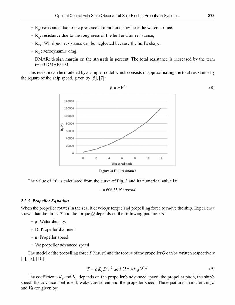
This resistor can be modeled by a simple model which consists in approximating the total resistance by

the square of the ship speed, given by [5], [7]:

2R a V (8)

Figure 3: Hull resistance

The value of “a” is calculated from the curve of Fig. 3 and its numerical value is:

a 606.53 / N noeud

2.2.5. Propeller Equation

When the propeller rotates in the sea, it develops torque and propelling force to move the ship. Experience

shows that the thrust T and the torque Q depends on the following parameters:

• : Water density.

• D: Propeller diameter

• n: Propeller speed.

• Va: propeller advanced speed

The model of the propelling force T (thrust) and the torque of the propeller Q can be written respectively

[5], [7], [10]:

4 2 TT K D n and5 2 QQ K D n (9)

The coefficients KT and K

Q depends on the propeller’s advanced speed, the propeller pitch, the ship’s

speed, the advance coefficient, wake coefficient and the propeller speed. The equations characterizing J

and Va are given by:


aV

J andnD

a 1 V V (10)

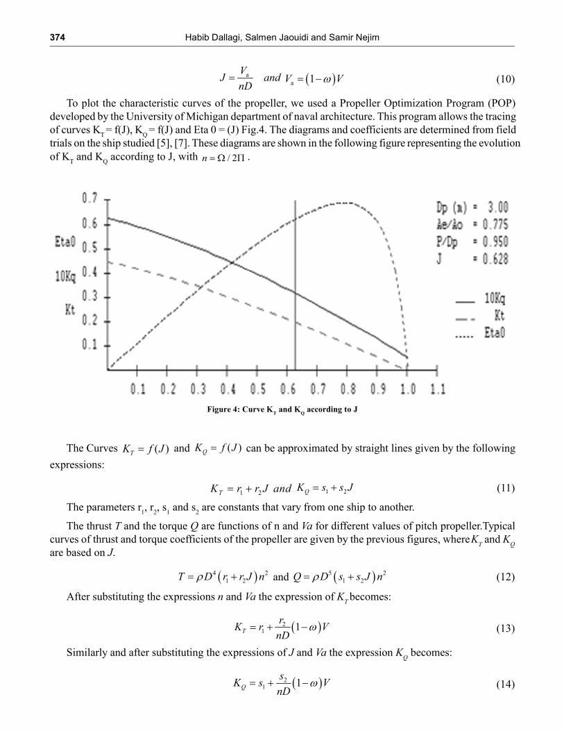
To plot the characteristic curves of the propeller, we used a Propeller Optimization Program (POP)

developed by the University of Michigan department of naval architecture. This program allows the tracing

of curves KT = f(J), K

Q = f(J) and Eta 0 = (J) Fig.4. The diagrams and coefficients are determined from field

trials on the ship studied [5], [7]. These diagrams are shown in the following figure representing the evolution

of KT and K

Q according to J, with / 2 n .

Figure 4: Curve KT and K

Q according to J

The Curves ( )TK f J and ( )QK f J can be approximated by straight lines given by the following

expressions:

1 2 TK r r J and 1 2 QK s s J (11)

The parameters r1, r

2, s

1 and s

2 are constants that vary from one ship to another.

The thrust T and the torque Q are functions of n and Va for different values of pitch propeller.Typical

curves of thrust and torque coefficients of the propeller are given by the previous figures, where KT and K

Q

are based on J.

4 2

1 2 T D r r J n and 5 2

1 2 Q D s s J n (12)

After substituting the expressions n and Va the expression of KT becomes:

21 1 T

rK r V

nD(13)

Similarly and after substituting the expressions of J and Va the expression KQ becomes:

21 1 Q

sK s V

nD(14)


By replacing the coefficients KT in the expression T of the propeller thrust T, the new expression of T is:

2 4 2 3

1 2 1 T r n D r n D V (15)

By replacing the coefficients KQ in the expression Q of the propulsion torque Q becomes, the new

expression of Q is:

2 5 2 4

1 21 Q s n D s n D V (16)

2.2.6. Ship motion equation

The ship floating on the sea surface is subjected to external and hydrodynamic forces. The propulsion

system comprises a motor coupled to a propeller shaft and a propeller with fixed blades. The equation of

vessel motion is given by the following relationship [10]:

1 ext

mV R t T T (17)

The equation of the shaft mechanical of the double star synchronous motor is:

m em f

I C Q Q (18)

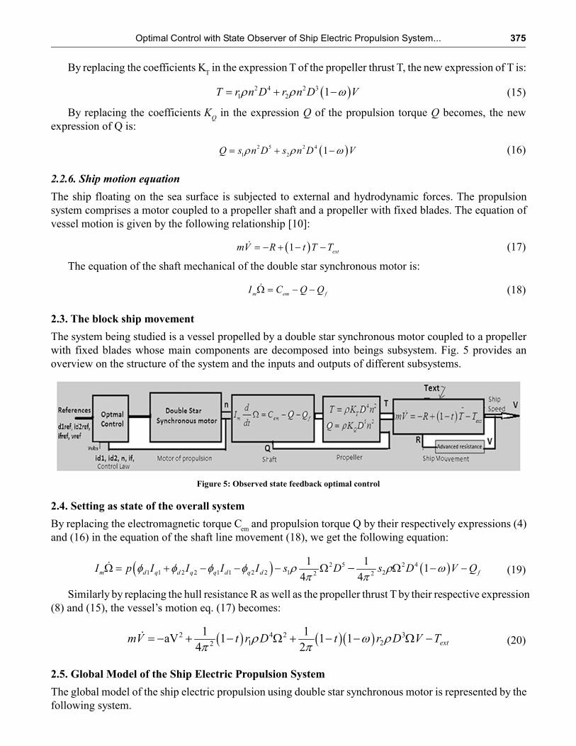
2.3. The block ship movement

The system being studied is a vessel propelled by a double star synchronous motor coupled to a propeller

with fixed blades whose main components are decomposed into beings subsystem. Fig. 5 provides an

overview on the structure of the system and the inputs and outputs of different subsystems.

2.4. Setting as state of the overall system

By replacing the electromagnetic torque Cem

and propulsion torque Q by their respectively expressions (4)

and (16) in the equation of the shaft line movement (18), we get the following equation:

2 5 2 4

1 1 2 2 1 1 2 2 1 22 2

1 11

4 4

m d q d q q d q d fI p I I I I s D s D V Q (19)

Similarly by replacing the hull resistance R as well as the propeller thrust T by their respective expression

(8) and (15), the vessel’s motion eq. (17) becomes:

2 4 2 31 22

1 1aV 1 1 1

4 2

extmV t r D t r D V T (20)

2.5. Global Model of the Ship Electric Propulsion System

The global model of the ship electric propulsion using double star synchronous motor is represented by the

following system.

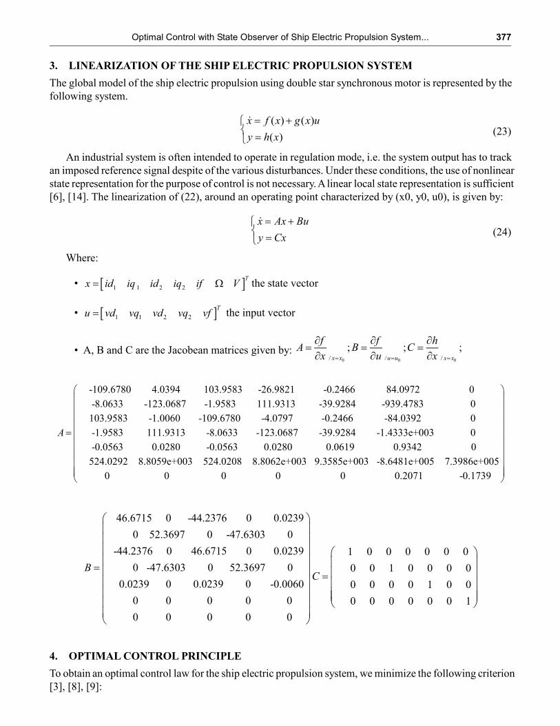
Figure 5: Observed state feedback optimal control


1 2

1 2 2

1 2

1 2 2

1 2

2 2 2

1 2

2 2 2

1 2

11

( )

1

d d d d fd

d dd d

q qq q

q q

d d d d fd

d dd d

q qq q

q q

f fd d d

f

qdm

d dL M Md difdt dtid

dt L M dtL M

d dL Md dt dtiq

dt L M

d dM L Md difdt dtid

dt L M dtM L

d dM Ld dt dtiq

dt M L

d d dM i id dt dt dtif

dt L

dp I

dt I

2 5 2 42 1 2 1 22 1 2 2 2

2 4 2 31 22

1 11

4 4

1 1 1aV 1 1 1

24

q q qd d d f

ext

I I I s D s D V Q

dVt r D t r D V T

dt m

(21)

By replacing the eq. (2) in eq. (21) it yields the system (22). Thus there was obtained a highly non-linear

system of order seven. The parameters of the system are given the in appendix.

11 1 2 1 3 2 4 2 5 6 1 7 2 8

11 1 2 1 3 2 4 2 5 6 1 7 2

21 1 2 1 3 2 4 2 5 6 1 7 2 8

21 1 2 1 3 2 4 2 5 6

d q d q f d d f

d q d q f q q

d q d q f d d f

d q d q f

didk I k I k I k I k I k V k V k V

dt

diql I l I l I l I l I l V l V

dt

didm I m I m I m I m I m V m V m V

dt

diqn I n I n I n I n I n V

dt1 7 2

1 1 2 1 3 2 4 2 5 6 1 7 2 8

1 1 1 2 2 1 3 1 4 2 5 2 2 6 1 2 7 8 9

1 2 3 4

² ²

² ²

q q

f

d q d q f d d f

d q d q f q f q d q d q

n V

dip I p I p I p I p I p V p V p V

dt

dq I I q I I q I I q I I q I I q I I q q V q

dt

dVt V t t V t

dt

(22)


3. LINEARIZATION OF THE SHIP ELECTRIC PROPULSION SYSTEM

The global model of the ship electric propulsion using double star synchronous motor is represented by the

following system.

( ) ( )

( )

x f x g x u

y h x(23)

An industrial system is often intended to operate in regulation mode, i.e. the system output has to track

an imposed reference signal despite of the various disturbances. Under these conditions, the use of nonlinear

state representation for the purpose of control is not necessary. A linear local state representation is sufficient

[6], [14]. The linearization of (22), around an operating point characterized by (x0, y0, u0), is given by:

x Ax Bu

y Cx(24)

Where:

• 1 1 2 2 T

x id iq id iq if V the state vector

• 1 1 2 2T

u vd vq vd vq vf the input vector

• A, B and C are the Jacobean matrices given by: 0 0 0/ / /

; ; ;

x x u u x x

f f hA B C

x u x

-109.6780 4.0394 103.9583 -26.9821 -0.2466 84.0972 0

-8.0633 -123.0687 -1.9583 111.9313 -39.9284

A

-939.4783 0

103.9583 -1.0060 -109.6780 -4.0797 -0.2466 -84.0392 0

-1.9583 111.9313 -8.0633 -123.0687 -39.9284 -1.4333e+003 0

-0.0563 0.0280 -0.0563 0.0280 0.0619 0.9342 0

524.0292 8.8059e+003 524.0208 8.8062e+003 9.3585e+003 -8.6481e+005 7.3986e+005

0 0 0 0 0 0.2071 -0.1739

46.6715 0 -44.2376 0 0.0239

0 52.3697 0 -47.6303 0

-44.2376 0 46.6715 0 0.0239

0 -47.6303 0 52.369B 7 0

0.0239 0 0.0239 0 -0.0060

0 0 0 0 0

0 0 0 0 0

1 0 0 0 0 0 0

0 0 1 0 0 0 0

0 0 0 0 1 0 0

0 0 0 0 0 0 1

C

4. OPTIMAL CONTROL PRINCIPLE

To obtain an optimal control law for the ship electric propulsion system, we minimize the following criterion

[3], [8], [9]:


0

1( )

2

T TJ u R u Q dt

(25)

With: R a symmetric positive definite matrix, Q a symmetric non-negative definite matrix. The control

law is then given by:

( ) ( ) ( )u t Fe t Kx t (26)

Where: ( ) ( ) ( )t e t y t is the difference between the reference and the output vector..

With 1ref 2ref ref frefe(t)= id id v iT

the reference vector

The gain F is given by:

1 1 1( )T T TF R B A PBR B PCQ (27)

The gain K is given by the equation:

1 TK R B P (28)

Where P is the solution of the Riccati equation:

1 0T TP PA A P PBR B P Q (29)

with TQ C QC

5. SHIP SPEED STATE OBSERVER

To design the sate feedback optimal control law, it is necessary to reconstruct the ship speed V in order to

be controlled. For this purpose, we propose a linear state observer using the output vector

1 2y(t)= id idT

if n and the input vector d d 1 21 2u(t)= u u

T

q q fu u u

The structure of a Luenberger observer is given by:

ˆ ˆ ˆ( )

ˆ ˆ

x Ax Bu L y y

y Cx

(30)

Where: is the output vector of the state observer. The matrix L is the observer gain. This structure can

be written in this form:

ˆˆ ˆx Ax Bu Ly (31)

with A A LC

To have an asymptotic convergence of the observed state towards the real state, it is necessary to

choose the gain L such that the matrix (A–LC) has negative real part eigen values. The control law using the

state observer is presented as follows [8], [9]:

ˆ( ) ( ) ( )u t Fe t Kx t (32)

6. NUMERICAL SIMULATION RESULTS

The Q and R matrices are chosen as follows:


1 0 0 0 0

0 1 0 0 0

0 0 1 0 0

0 0 0 1 0

0 0 0 0 1

R

1 0 0 0

0 1 0 0

0 0 1 0

0 0 0 1

Q

The gain of the optimal control Kopt obtained is the following:

0.2156 -0.0270 0.0123 -0.0491 0.5529 0.0001 9.9110

0.2804 -0.0689 0.2750 -0.1089 0.1815 0.0003 12.6652

0.0297 -0.0326 0.2339 -0.0450 0.5552 0optK .0001 10.4330

-0.4321 0.1126 -0.4269 0.1746 0.0328 -0.0004 -12.5267

0.0024 -0.0007 0.0024 -0.0011 -0.1366 0.0000 -1.4717

The gain matrix of the observer obtained L is:

-33.1224 -38.1385 3.7903 0

-4.4125 2.0247e+003 -77.9131 0

115.8725 32.9322 -2.4066 0

-60.0017 1.9653e+003 -77.0144 L 0

-0.1563 -4.5709 0.1902 0

471.5962 611.1918 9.3571e+003 0

-0.0077 -6.7310 -0.0170 0

Figure 6: Observed state feedback optimal control


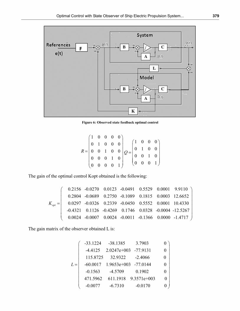
The reference gain matrix F obtained by the resolution of the eq. (27):

-0.0128 -0.0120 -0.7868 24.2730

-0.0225 -0.0225 5.1470 -64.2004

-0.0130 -0.0139 -0.4640 22.0222

0.0165 0.0166 -7.2765 22.0306

0.0016 0.0016 0.7343 -9.78

F

74

The transition matrix P determined from the Riccati equation is:

0.0514 -0.0124 0.0493 -0.0196 0.0038 4.6558e-005 1.6386

-0.0124 0.0037 -0.0125 0.0055

P

0.0234 -1.3096e-005 0.1406

0.0493 -0.0125 0.0518 -0.0195 0.0038 4.6117e-005 1.6444

-0.0196 0.0055 -0.0195 0.0083 0.0219 -1.9839e-005 -0.1113

0.0038 0.0234 0.0038 0.0219 22.7619 2.4780e-005 258.0307

4.6558e-005 -1.3096e-005 4.6117e-005 -1.9839e-005 2.4780e-005 4.7843e-008 0.0028

1.6386 0.1406 1.6444 -0.1113 258.0307 0.0028 1.0270e+004

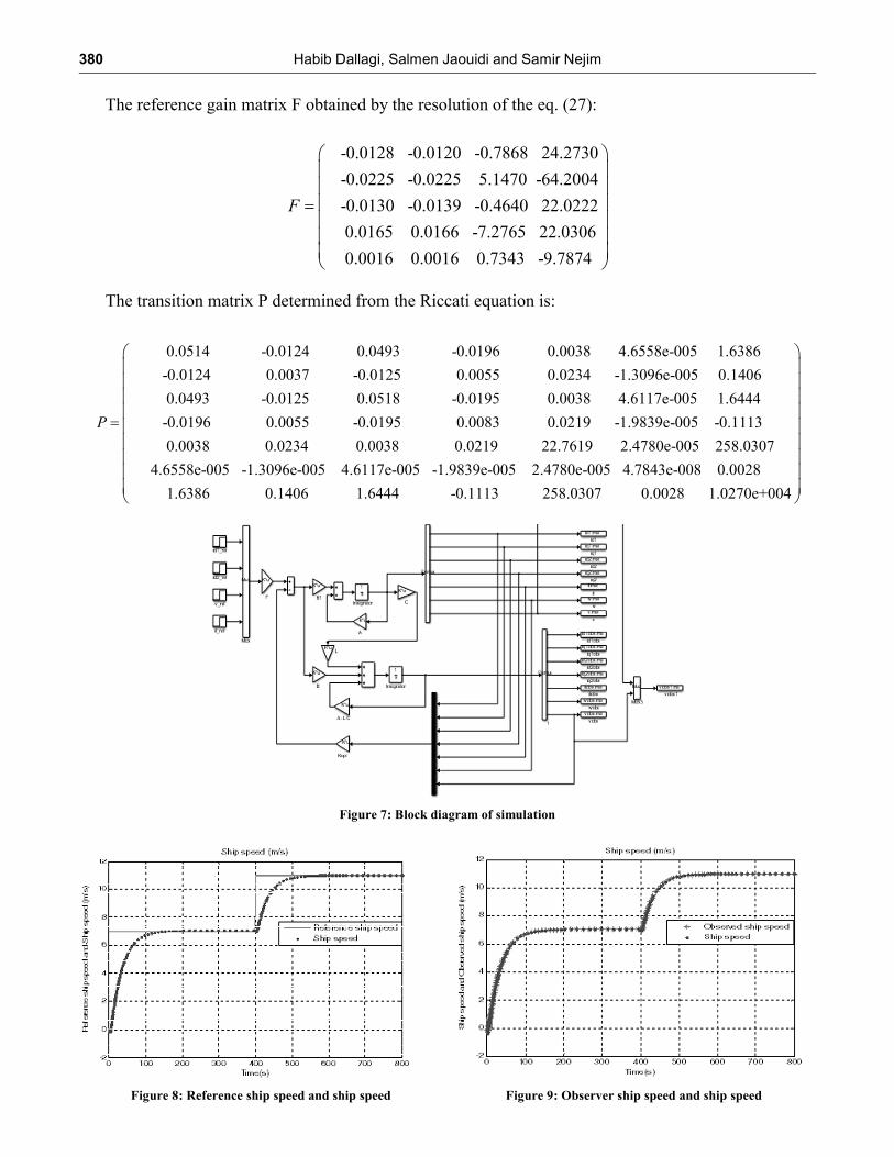
Figure 7: Block diagram of simulation

Figure 8: Reference ship speed and ship speed Figure 9: Observer ship speed and ship speed


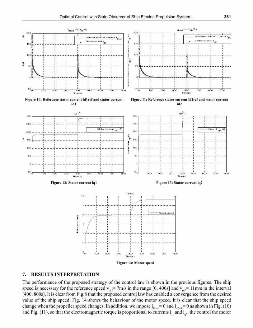
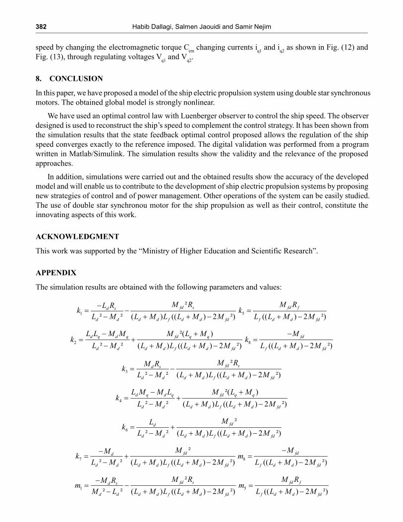
Figure 10: Reference stator current id1ref and stator current

id1

Figure 11: Reference stator current id2ref and stator current

id2

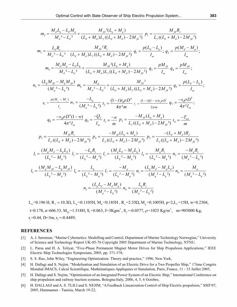
Figure 12: Stator current iq1 Figure 13: Stator current iq2

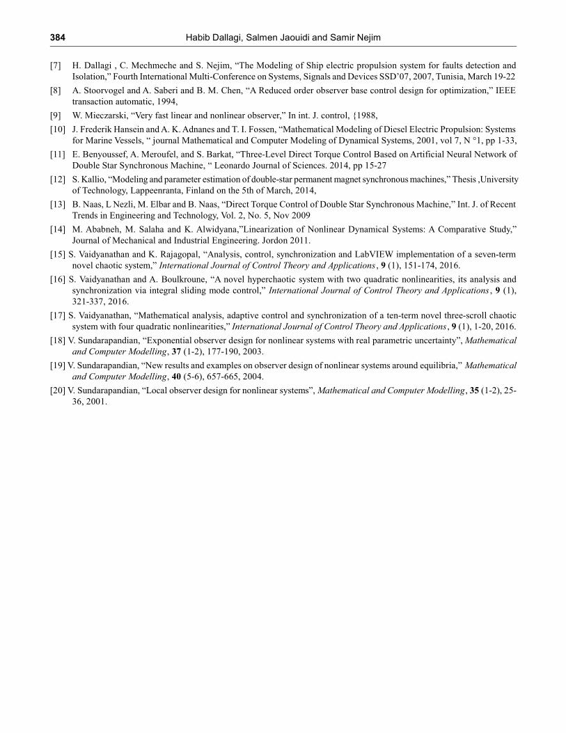
Figure 14: Motor speed

7. RESULTS INTERPRETATION

The performance of the proposed strategy of the control law is shown in the previous figures. The ship

speed is necessary for the reference speed vre f

= 7m/s in the range [0, 400s] and vref

= 11m/s in the interval

[400, 800s]. It is clear from Fig.8 that the proposed control law has enabled a convergence from the desired

value of the ship speed. Fig. 14 shows the behaviour of the motor speed. It is clear that the ship speed

change when the propeller speed changes. In addition, we impose id1ref

= 0 and id2ref

= 0 as shown in Fig. (10)

and Fig. (11), so that the electromagnetic torque is proportional to currents iq1

and iq2

, the control the motor


speed by changing the electromagnetic torque Cem

changing currents iq1

and iq2

as shown in Fig. (12) and

Fig. (13), through regulating voltages Vq1

and Vq2

.

8. CONCLUSION

In this paper, we have proposed a model of the ship electric propulsion system using double star synchronous

motors. The obtained global model is strongly nonlinear.

We have used an optimal control law with Luenberger observer to control the ship speed. The observer

designed is used to reconstruct the ship’s speed to complement the control strategy. It has been shown from

the simulation results that the state feedback optimal control proposed allows the regulation of the ship

speed converges exactly to the reference imposed. The digital validation was performed from a program

written in Matlab/Simulink. The simulation results show the validity and the relevance of the proposed

approaches.

In addition, simulations were carried out and the obtained results show the accuracy of the developed

model and will enable us to contribute to the development of ship electric propulsion systems by proposing

new strategies of control and of power management. Other operations of the system can be easily studied.

The use of double star synchronou motor for the ship propulsion as well as their control, constitute the

innovating aspects of this work.

ACKNOWLEDGMENT

This work was supported by the “Ministry of Higher Education and Scientific Research”.

APPENDIX

The simulation results are obtained with the following parameters and values:

1

²

² ² ( ) (( ) 2 ²)

fd sd s

d d d d f d d fd

M RL Rk

L M L M L L M M

5

(( ) 2 ²)

fd f

f d d fd

M Rk

L L M M

2

²( )

² ² ( ) (( ) 2 ²)

d q d q fd q q

d d d d f d d fd

L L M M M L Mk

L M L M L L M M

8

(( ) 2 ²)

fd

f d d fd

Mk

L L M M

3

²

² ² ( ) (( ) 2 ²)

fd sd s

d d d d f d d fd

M RM Rk

L M L M L L M M

4

²( )

² ² ( ) (( ) 2 ²)

d q d q fd q q

d d d d f d d fd

L M M L M L Mk

L M L M L L M M

6

²

² ² ( ) (( ) 2 ²)

fdd

d d d d f d d fd

MLk

L M L M L L M M

7

²

² ² ( ) (( ) 2 ²)

fdd

d d d d f d d fd

MMk

L M L M L L M M

8

(( ) 2 ²)

fd

f d d fd

Mm

L L M M

1

²

² ² ( ) (( ) 2 ²)

fd sd s

d d d d f d d fd

M RM Rm

M L L M L L M M

5

(( ) 2 ²)

fd f

f d d fd

M Rm

L L M M


2

²( )

² ² ( ) (( ) 2 ²)

d q d q fd q q

d d d d f d d fd

M L L M M L Mm

M L L M L L M M

1

(( ) 2 ²)

fd s

f d d fd

M Rp

L L M M

3

²

² ² ( ) (( ) 2 ²)

fd sd s

d d d d f d d fd

M RL Rm

M L L M L L M M

1

( );

d q

m

p L Lq

I

2

( );

d q

m

p M Mq

I

4

²( )

² ² ( ) (( ) 2 ²)

d q d q fd q q

d d d d f d d fd

M M L L M L Mm

M L L M L L M M

3

fd

m

pMq

I 4 ;

fd

m

pMq

I

5

( )

( ² ²)

q fd q fd

q q

L M M Mn

M L

6

²

² ² ( ) (( ) 2 ²)

fdd

d d d d f d d fd

MMm

M L L M L L M M

5

( );

d q

m

p L Lq

I

6

( )d q

m

p M Mq

I

7

( ² ²)

q

q q

Ln

M L

4

12

(1 )

4 ²

t r Dt

m

3

2

3

(1 )(1 )

2

t w r Dt

m

5

17 ;

4 ² m

s Dq

I

4

28

(1 )

4 ² m

s D wq

I

9

f

m

Qq

I

1

at

m

2

( )

(( ) 2 ²)

fd q q

f d d fd

M L Mp

L L M M

4extT

tm

3(( ) 2 ²)

fd s

f d d fd

M Rp

L L M M

4

( )

(( ) 2 ²)

fd q q

f d d fd

M L Mp

L L M M

5

( )

(( ) 2 ²)

d d f

f d d fd

L M Rp

L L M M

1

( )

( ² ²)

q d q d

q q

M M L Ll

L M

2

( ² ²)

q s

q q

L Rl

L M

3

( )

( ² ²)

q d d q

q q

M L M Ll

L M

4

( ² ²)

q s

q q

M Rl

L M

2

( ² ²)

q s

q q

M Rn

M L

5

( )

( ² ²)

q fd q fd

q q

M M L Ml

L M

6

( ² ²)

q

q q

Ll

L M

7

( ² ²)

q

q q

Ml

L M

1

( )

( ² ²)

q d q d

q q

L M M Ln

M L

6

( ² ²)

q

q q

Mn

M L

3

( )

( ² ²)

q d d q

q q

L L M Mn

M L

4

( ² ²)

q s

q q

L Rn

M L

d f q d s q f

2 3

fd 1 2

1 2

L =0.196 H, R 10.3 , L =0.1105H, M =0.185H , R =2.35 , M =0.1005H, p=2,L =15H, w=0.2304,

t=0.178, a=606.53, M =1.518H, S =0.063, J=3Kgm , S =-0.0577, =1025 Kg/m , m=905000 Kg,

r =0.44, D=3m, r =-0.4489;

REFERENCES

[1] A. J. Sørensen, “Marine Cybernetics: Modelling and Control, Department of Marine Technology Norwegian,” University

of Science and Technology Report UK-05-76 Copyright 2005 Department of Marine Technology, NTNU.

[2] L. Parsa and H. A. Toliyat, “Five-Phase Permanent Magnet Motor Drives for Ship Propulsion Applications,” IEEE

Electric Ship Technologies Symposium, 2005, pp. 371-378,

[3] S. S. Rao, John Wiley, “Engineering Optimization: Theory and practice,” 1996, New York,

[4] H. Dallagi and S. Nejim, “Modelisation and Simulation of an Electric Drive for a Two Propeller Ship,” 17ème Congrès

Mondial IMACS, Calcul Scientifique, Mathématiques Appliquées et Simulation, Paris, France, 11 - 15 Juillet 2005,

[5] H. Dallagi and S. Nejim, “Optimization of an Integrated Power System of an Electric Ship,” International Conference on

ship propulsion and railway traction systems, Bologna-Italy, 2006, 4, 5, 6 Octobre,

[6] H. DALLAGI and A. S. TLILI and S. NEJIM, “A Feedback Linearization Control of Ship Electric propulsion,” SSD’07,

2005, Hammamet - Tunisia, March 19-22,


[7] H. Dallagi , C. Mechmeche and S. Nejim, “The Modeling of Ship electric propulsion system for faults detection and

Isolation,” Fourth International Multi-Conference on Systems, Signals and Devices SSD’07, 2007, Tunisia, March 19-22

[8] A. Stoorvogel and A. Saberi and B. M. Chen, “A Reduced order observer base control design for optimization,” IEEE

transaction automatic, 1994,

[9] W. Mieczarski, “Very fast linear and nonlinear observer,” In int. J. control, {1988,

[10] J. Frederik Hansein and A. K. Adnanes and T. I. Fossen, “Mathematical Modeling of Diesel Electric Propulsion: Systems

for Marine Vessels, “ journal Mathematical and Computer Modeling of Dynamical Systems, 2001, vol 7, N °1, pp 1-33,

[11] E. Benyoussef, A. Meroufel, and S. Barkat, “Three-Level Direct Torque Control Based on Artificial Neural Network of

Double Star Synchronous Machine, “ Leonardo Journal of Sciences. 2014, pp 15-27

[12] S. Kallio, “Modeling and parameter estimation of double-star permanent magnet synchronous machines,” Thesis ,University

of Technology, Lappeenranta, Finland on the 5th of March, 2014,

[13] B. Naas, L Nezli, M. Elbar and B. Naas, “Direct Torque Control of Double Star Synchronous Machine,” Int. J. of Recent

Trends in Engineering and Technology, Vol. 2, No. 5, Nov 2009

[14] M. Ababneh, M. Salaha and K. Alwidyana,”Linearization of Nonlinear Dynamical Systems: A Comparative Study,”

Journal of Mechanical and Industrial Engineering. Jordon 2011.

[15] S. Vaidyanathan and K. Rajagopal, “Analysis, control, synchronization and LabVIEW implementation of a seven-term

novel chaotic system,” International Journal of Control Theory and Applications , 9 (1), 151-174, 2016.

[16] S. Vaidyanathan and A. Boulkroune, “A novel hyperchaotic system with two quadratic nonlinearities, its analysis and

synchronization via integral sliding mode control,” International Journal of Control Theory and Applications , 9 (1),

321-337, 2016.

[17] S. Vaidyanathan, “Mathematical analysis, adaptive control and synchronization of a ten-term novel three-scroll chaotic

system with four quadratic nonlinearities,” International Journal of Control Theory and Applications , 9 (1), 1-20, 2016.

[18] V. Sundarapandian, “Exponential observer design for nonlinear systems with real parametric uncertainty”, Mathematical

and Computer Modelling, 37 (1-2), 177-190, 2003.

[19] V. Sundarapandian, “New results and examples on observer design of nonlinear systems around equilibria,” Mathematical

and Computer Modelling, 40 (5-6), 657-665, 2004.

[20] V. Sundarapandian, “Local observer design for nonlinear systems”, Mathematical and Computer Modelling, 35 (1-2), 25-

36, 2001.

Documents

Optimal Control with State Observer of - serialsjournals.com · Optimal Control with State Observer of ... in three-phase stator winding (a1, b1, c1, a2, b2, c2) of a two-phase model