Embed Size (px)
Citation preview

Optimal control of treatment time
in a diffuse interface model of tumor growth and related issues
E. Rocca
Universita degli Studi di Pavia
June 28, 2018 – MOX - Politecnico di Milano
joint works with Harald Garcke (Regensburg)-Kei Fong Lam (Hong-Kong)
and Sergio Frigeri (Brescia)-Kei Fong Lam (Hong-Kong)-Giulio Schimperna (Pavia)
Fondazione Cariplo and Regione Lombardia Grant MEGAsTaR 2016-2019
E. Rocca (Universita degli Studi di Pavia) Diffuse interface models of tumor growth June 28,2018 1 / 46

Outline
1 Phase field models for tumor growth
2 The optimal control problem
3 First order optimality conditions
4 Some simulations
5 A multispecies model with velocity
6 Perspectives and Open problems
E. Rocca (Universita degli Studi di Pavia) Diffuse interface models of tumor growth June 28,2018 2 / 46
Outline
1 Phase field models for tumor growth
2 The optimal control problem
3 First order optimality conditions
4 Some simulations
5 A multispecies model with velocity
6 Perspectives and Open problems
E. Rocca (Universita degli Studi di Pavia) Diffuse interface models of tumor growth June 28,2018 3 / 46

Setting
Tumors grown in vitro often exhibit “layered” structures:
Figure: Zhang et al. Integr. Biol., 2012, 4, 1072–1080. Scale bar 100µm = 0:1mm
A continuum thermodynamically consistent model is introduced with the ansatz:
sharp interfaces are replaced by narrow transition layers arising due to adhesive forces
among the cell species: a diffuse interface separates tumor and healthy cell regions
proliferating tumor cells surrounded by (healthy) host cells, and a nutrient (e.g.
glucose)
E. Rocca (Universita degli Studi di Pavia) Diffuse interface models of tumor growth June 28,2018 4 / 46

Diffuse interfaces
E. Rocca (Universita degli Studi di Pavia) Diffuse interface models of tumor growth June 28,2018 5 / 46

Advantages of diffuse interfaces in tumor growth models
It eliminates the need to enforce complicated boundary conditions across the
tumor/host tissue and other species/species interfaces
It eliminates the need to explicitly track the position of interfaces, as is required in
the sharp interface framework
The mathematical description remains valid even when the tumor undergoes
toplogical changes (e.g. metastasis)
Regarding modeling of diffuse interface tumor growth we can quote, e.g.,
Ciarletta, Cristini, Frieboes, Garcke, Hawkins, Hilhorst, Lam, Lowengrub, Oden,
Wise, also for their numerical simulations → complex changes in tumor
morphologies due to the interactions with nutrients or toxic agents and also due to
mechanical stresses
Frieboes, Jin, Chuang, Wise, Lowengrub, Cristini, Garcke, Lam, Nurnberg, Sitka, for
the interaction of multiple tumor cell species described by multiphase mixture models
E. Rocca (Universita degli Studi di Pavia) Diffuse interface models of tumor growth June 28,2018 6 / 46

Theoretical analysis: two-phase models
In terms of the theoretical analysis most of the recent literature is restricted to the
two-phase variant, i.e., to models that only account for the evolution of a tumor
surrounded by healthy tissue.
In this setting, there is no differentiation among the tumor cells that exhibit
heterogeneous growth behavior. Hence this kind of two-phase models are just able to
describe the growth of a young tumor before the onset of quiescence and necrosis.
Analytical results related to well-posedness, asymptotic limits and long-timebehavior, but also optimal control and sliding modes, have been established in anumber of papers of a number of authors which include: Agosti, Ciarletta, Colli,Frigeri, Garcke, Gilardi, Grasselli, Hilhorst, Lam, Marinoschi, Melchionna, E.R.,Scala, Sprekels Wu, etc...
I for tumor growth models based on the coupling of Cahn–Hilliard (for the tumor
density) and reaction–diffusion (for the nutrient) equations, and
I for models of Cahn–Hilliard–Darcy type.
E. Rocca (Universita degli Studi di Pavia) Diffuse interface models of tumor growth June 28,2018 7 / 46

Optimization over the treatment time: H. Garcke, K.F. Lam, E. Rocca,
Applied Mathematics & Optimization, 2017
Common treatment for tumors are
Chemotheraphy
Radiation therapy
Surgery
For treatment involving drugs, the patient is given several doses of drugs over a few days,
followed by a rest period of 3 - 4 weeks, and the cycle is repeated. Goal is to shrink the
tumor into a more manageable size for which surgery can be applied.
Unfortunately, cytotoxic drugs also harms the healthy host tissues, and can accumulate in
the body. Furthermore, drug clearance may also cause damage to various vital organs
(e.g. kidneys and liver).
Worst case scenario: Cytotoxins may have cancer-causing effects, and tumor cells can
mutate to become resistant to the drug.
Thus, aside from optimising the drug distribution, we should also consider optimising the
treatment time.
E. Rocca (Universita degli Studi di Pavia) Diffuse interface models of tumor growth June 28,2018 8 / 46

Cahn–Hilliard + nutrient models with source terms
The simplest phase field model is a Cahn–Hilliard system with source terms for ϕ: the
difference in volume fractions (ϕ = 1: tumor phase, ϕ = −1: healthy tissue phase):
∂tϕ = ∆µ+M, µ = Ψ′(ϕ)−∆ϕ
The source term M accounts for biological mechanisms related to proliferation and
death. Introduce a Reaction-diffusion equation for the nutrient proportion σ:
∂tσ = ∆σ − S
where S models interaction with the tumor cells
In [Chen, Wise, Shenoy, Lowengrub (2014)], [Garcke, Lam, Sitka, Styles (2016)]:
M = h(ϕ)(Pσ −A), S = h(ϕ)Cσ
Here h(s) is an interpolation function such that h(−1) = 0 and h(1) = 1, andI h(ϕ)Pσ - proliferation of tumor cells proportional to nutrient concentrationI h(ϕ)A - apoptosis of tumor cellsI h(ϕ)Cσ - consumption of nutrient by the tumor cells
A regular double-well potential Ψ, e.g., Ψ(s) = 1/4(1− s2)2
E. Rocca (Universita degli Studi di Pavia) Diffuse interface models of tumor growth June 28,2018 9 / 46

Cahn–Hilliard + nutrient models with source terms
The simplest phase field model is a Cahn–Hilliard system with source terms for ϕ: the
difference in volume fractions (ϕ = 1: tumor phase, ϕ = −1: healthy tissue phase):
∂tϕ = ∆µ+M, µ = Ψ′(ϕ)−∆ϕ
The source term M accounts for biological mechanisms related to proliferation and
death.
Introduce a Reaction-diffusion equation for the nutrient proportion σ:
∂tσ = ∆σ − S
where S models interaction with the tumor cells
In [Chen, Wise, Shenoy, Lowengrub (2014)], [Garcke, Lam, Sitka, Styles (2016)]:
M = h(ϕ)(Pσ −A), S = h(ϕ)Cσ
Here h(s) is an interpolation function such that h(−1) = 0 and h(1) = 1, andI h(ϕ)Pσ - proliferation of tumor cells proportional to nutrient concentrationI h(ϕ)A - apoptosis of tumor cellsI h(ϕ)Cσ - consumption of nutrient by the tumor cells
A regular double-well potential Ψ, e.g., Ψ(s) = 1/4(1− s2)2
E. Rocca (Universita degli Studi di Pavia) Diffuse interface models of tumor growth June 28,2018 9 / 46

Cahn–Hilliard + nutrient models with source terms
The simplest phase field model is a Cahn–Hilliard system with source terms for ϕ: the
difference in volume fractions (ϕ = 1: tumor phase, ϕ = −1: healthy tissue phase):
∂tϕ = ∆µ+M, µ = Ψ′(ϕ)−∆ϕ
The source term M accounts for biological mechanisms related to proliferation and
death. Introduce a Reaction-diffusion equation for the nutrient proportion σ:
∂tσ = ∆σ − S
where S models interaction with the tumor cells
In [Chen, Wise, Shenoy, Lowengrub (2014)], [Garcke, Lam, Sitka, Styles (2016)]:
M = h(ϕ)(Pσ −A), S = h(ϕ)Cσ
Here h(s) is an interpolation function such that h(−1) = 0 and h(1) = 1, andI h(ϕ)Pσ - proliferation of tumor cells proportional to nutrient concentrationI h(ϕ)A - apoptosis of tumor cellsI h(ϕ)Cσ - consumption of nutrient by the tumor cells
A regular double-well potential Ψ, e.g., Ψ(s) = 1/4(1− s2)2
E. Rocca (Universita degli Studi di Pavia) Diffuse interface models of tumor growth June 28,2018 9 / 46

Cahn–Hilliard + nutrient models with source terms
The simplest phase field model is a Cahn–Hilliard system with source terms for ϕ: the
difference in volume fractions (ϕ = 1: tumor phase, ϕ = −1: healthy tissue phase):
∂tϕ = ∆µ+M, µ = Ψ′(ϕ)−∆ϕ
The source term M accounts for biological mechanisms related to proliferation and
death. Introduce a Reaction-diffusion equation for the nutrient proportion σ:
∂tσ = ∆σ − S
where S models interaction with the tumor cells
In [Chen, Wise, Shenoy, Lowengrub (2014)], [Garcke, Lam, Sitka, Styles (2016)]:
M = h(ϕ)(Pσ −A), S = h(ϕ)Cσ
Here h(s) is an interpolation function such that h(−1) = 0 and h(1) = 1, andI h(ϕ)Pσ - proliferation of tumor cells proportional to nutrient concentrationI h(ϕ)A - apoptosis of tumor cellsI h(ϕ)Cσ - consumption of nutrient by the tumor cells
A regular double-well potential Ψ, e.g., Ψ(s) = 1/4(1− s2)2
E. Rocca (Universita degli Studi di Pavia) Diffuse interface models of tumor growth June 28,2018 9 / 46

Outline
1 Phase field models for tumor growth
2 The optimal control problem
3 First order optimality conditions
4 Some simulations
5 A multispecies model with velocity
6 Perspectives and Open problems
E. Rocca (Universita degli Studi di Pavia) Diffuse interface models of tumor growth June 28,2018 10 / 46

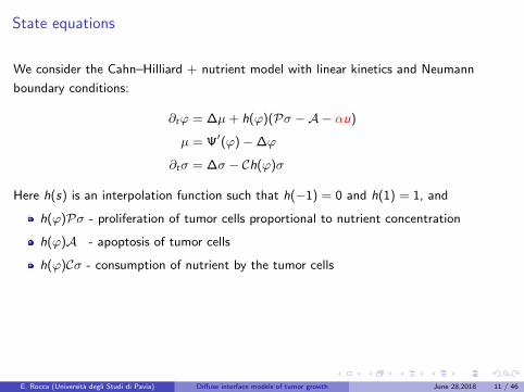
State equations
We consider the Cahn–Hilliard + nutrient model with linear kinetics and Neumann
boundary conditions:
∂tϕ = ∆µ+ h(ϕ)(Pσ −A− αu)
µ = Ψ′(ϕ)−∆ϕ
∂tσ = ∆σ − Ch(ϕ)σ
Here h(s) is an interpolation function such that h(−1) = 0 and h(1) = 1, and
h(ϕ)Pσ - proliferation of tumor cells proportional to nutrient concentration
h(ϕ)A - apoptosis of tumor cells
h(ϕ)Cσ - consumption of nutrient by the tumor cells
h(ϕ)αu - elimination of tumor cells by cytotoxic drugs at a constant rate α,
u acts as a control here. In applications u : [0,T ]→ [0, 1] is spatially constant,
where u = 1 represents full dosage, u = 0 represents no dosage
E. Rocca (Universita degli Studi di Pavia) Diffuse interface models of tumor growth June 28,2018 11 / 46

Objective functional
For positive βT , βu and non-negative βQ , βΩ, βS , we consider
J(ϕ, u, τ) :=
∫ τ
0
∫Ω
βQ2|ϕ− ϕQ |2 +
∫Ω
βΩ
2|ϕ(τ)− ϕΩ|2
+
∫Ω
βS2
(1 + ϕ(τ)) +
∫ τ
0
∫Ω
βu2|u|2 + βT τ
the variable τ denotes the unknown treatment time to be optimised,
ϕQ is a desired evolution of the tumor over the treatment,
ϕΩ is a desired final state of the tumor (stable equilibrium of the system),
the term 1+ϕ(τ)2
measures the size of the tumor at the end of the treatment,
the constant βT penalizes long treatment times.
Expectation: An optimal control will be a pair (u∗, τ∗) and we will obtain two optimality
conditions.
E. Rocca (Universita degli Studi di Pavia) Diffuse interface models of tumor growth June 28,2018 12 / 46

Regarding the terms appearing in the cost functional
J(ϕ, u, τ) :=
∫ τ
0
∫Ω
βQ2|ϕ− ϕQ |2 +
∫Ω
βΩ
2|ϕ(τ)− ϕΩ|2
+
∫Ω
βS2
(1 + ϕ(τ)) +
∫ τ
0
∫Ω
βu2|u|2 + βT τ
A large value of |ϕ− ϕQ |2 would mean that the patient suffers from the growth of
the tumor, and a large value of |u|2 would mean that the patient suffers from high
toxicity of the drug;
The function ϕΩ can be a stable configuration of the system, so that the tumor does
not grow again once the treatment is completed or a configuration which is suitable
for surgery;
The variable τ can be regarded as the treatment time of one cycle, i.e., the amount
of time the drug is applied to the patient before the period of rest, or the treatment
time before surgery;
It is possible to replace βT τ by a more general function f (τ) where f : R+ → R+ is
continuously differentiable and increasing.
E. Rocca (Universita degli Studi di Pavia) Diffuse interface models of tumor growth June 28,2018 13 / 46

Relaxed objective functional
However, we will not study the functional
J(ϕ, u, τ) :=
∫ τ
0
∫Ω
βQ2|ϕ− ϕQ |2 +
∫Ω
βΩ
2|ϕ(τ)− ϕΩ|2
+
∫Ω
βS2
(1 + ϕ(τ)) +
∫ τ
0
∫Ω
βu2|u|2 + βT τ
but a relaxed version - in order to keep a control u just bounded without requiring more
regularity
Let r > 0 be fixed and let T ∈ (0,∞) denote a fixed maximal time in which the patient
is allowed to undergo a treatment, we define
Jr (ϕ, u, τ) :=
∫ τ
0
∫Ω
βQ2|ϕ− ϕQ |2 +
1
r
∫ τ
τ−r
∫Ω
βΩ
2|ϕ− ϕΩ|2
+1
r
∫ τ
τ−r
∫Ω
βS2
(1 + ϕ) +
∫ T
0
∫Ω
βu2|u|2 + βT τ
E. Rocca (Universita degli Studi di Pavia) Diffuse interface models of tumor growth June 28,2018 14 / 46

Relaxed objective functional
Let r > 0 be fixed and let T ∈ (0,∞) denote a maximal time, we define
Jr (ϕ, u, τ) :=
∫ τ
0
∫Ω
βQ2|ϕ− ϕQ |2 +
1
r
∫ τ
τ−r
∫Ω
βΩ
2|ϕ− ϕΩ|2
+1
r
∫ τ
τ−r
∫Ω
βS2
(1 + ϕ) +
∫ T
0
∫Ω
βu2|u|2 + βT τ.
The optimal control problem is
min(ϕ,u,τ)
Jr (ϕ, u, τ)
subject to τ ∈ (0,T ), u ∈ Uad = f ∈ L∞(Ω× (0,T )) : 0 ≤ f ≤ 1, and
∂tϕ = ∆µ+ h(ϕ)(Pσ −A− αu) in Ω× (0,T ) = Q,
µ = Ψ′(ϕ)−∆ϕ in Q,
∂tσ = ∆σ − Ch(ϕ)σ in Q,
0 = ∂nϕ = ∂nσ = ∂nµ on ∂Ω× (0,T ),
ϕ(0) = ϕ0, σ(0) = σ0 in Ω.
E. Rocca (Universita degli Studi di Pavia) Diffuse interface models of tumor growth June 28,2018 15 / 46

Well-posedness of state equations
Theorem
Let ϕ0 ∈ H3, σ0 ∈ H1 with 0 ≤ σ0 ≤ 1, h ∈ C 0,1(R) ∩ L∞(R) non-negative, and Ψ is a
quartic potential, then for every u ∈ Uad there exists a unique triplet
ϕ ∈ L∞(0,T ;H2) ∩ L2(0,T ;H3) ∩ H1(0,T ; L2) ∩ C 0(Q),
µ ∈ L2(0,T ;H2) ∩ L∞(0,T ; L2),
σ ∈ L∞(0,T ;H1) ∩ L2(0,T ;H2) ∩ H1(0,T ; L2), 0 ≤ σ ≤ 1 a.e. in Q
satisfying the state equations.
Key points:
Boundedness of σ comes from a weak comparison principle applied to
∂tσ = ∆σ − Ch(ϕ)σ
and it is an essential ingredient for the existence proof
Proof utilises a Schauder fixed point argument
E. Rocca (Universita degli Studi di Pavia) Diffuse interface models of tumor growth June 28,2018 16 / 46

Existence of a minimiser
Using that ϕ ∈ L1(0,T ; L1), Jr is bounded from below:
Jr (ϕ, u, τ) :=
∫ τ
0
∫Ω
βQ2|ϕ− ϕQ |2 +
1
r
∫ τ
τ−r
∫Ω
βΩ
2|ϕ− ϕΩ|2
+1
r
∫ τ
τ−r
∫Ω
βS2
(1 + ϕ) +
∫ T
0
∫Ω
βu2|u|2 + βT τ
≥ −βS2r
∫ τ
τ−r
∫Ω
|ϕ| ≥ −βS2r‖ϕ‖L1(0,T ;L1) ≥ −C .
Minimising sequence (un, τn) ∈ Uad × (0,T ), with corresponding state variables
(ϕn, µn, σn) such that
limn→∞
Jr (ϕn, un, τn) = inf(φ,w,s)
Jr (φ,w , s).
We extract a convergent subsequence un ∗ u∗ ∈ L∞(Q) and limit functions
(ϕ∗, µ∗, σ∗) satisfying the state equations and
ϕn → ϕ∗ in C 0([0,T ]; L2) ∩ L2(Q).
As τnn∈N is a bounded sequence, we extract a convergent subsequence
τn → τ∗ ∈ [0,T ].
E. Rocca (Universita degli Studi di Pavia) Diffuse interface models of tumor growth June 28,2018 17 / 46

Existence of a minimiser
Using that ϕ ∈ L1(0,T ; L1), Jr is bounded from below:
Jr (ϕ, u, τ) ≥ −βS2r
∫ τ
τ−r
∫Ω
|ϕ| ≥ −βS2r‖ϕ‖L1(0,T ;L1) ≥ −C .
Minimising sequence (un, τn) ∈ Uad × (0,T ), with corresponding state variables
(ϕn, µn, σn) such that
limn→∞
Jr (ϕn, un, τn) = inf(φ,w,s)
Jr (φ,w , s).
We extract a convergent subsequence un ∗ u∗ ∈ L∞(Q) and limit functions
(ϕ∗, µ∗, σ∗) satisfying the state equations and
ϕn → ϕ∗ in C 0([0,T ]; L2) ∩ L2(Q).
Key point: All of the convergence are with respect to the interval [0,T ].
As τnn∈N is a bounded sequence, we extract a convergent subsequence
τn → τ∗ ∈ [0,T ].
E. Rocca (Universita degli Studi di Pavia) Diffuse interface models of tumor growth June 28,2018 17 / 46

Existence of a minimiser
Using that ϕ ∈ L1(0,T ; L1), Jr is bounded from below:
Jr (ϕ, u, τ) ≥ −βS2r
∫ τ
τ−r
∫Ω
|ϕ| ≥ −βS2r‖ϕ‖L1(0,T ;L1) ≥ −C .
Minimising sequence (un, τn) ∈ Uad × (0,T ), with corresponding state variables
(ϕn, µn, σn) such that
limn→∞
Jr (ϕn, un, τn) = inf(φ,w,s)
Jr (φ,w , s).
We extract a convergent subsequence un ∗ u∗ ∈ L∞(Q) and limit functions
(ϕ∗, µ∗, σ∗) satisfying the state equations and
ϕn → ϕ∗ in C 0([0,T ]; L2) ∩ L2(Q).
As τnn∈N is a bounded sequence, we extract a convergent subsequence
τn → τ∗ ∈ [0,T ].
E. Rocca (Universita degli Studi di Pavia) Diffuse interface models of tumor growth June 28,2018 17 / 46

Existence of minimiser
To pass to the limit in:
Jr (ϕn, un, τn) :=
∫ τn
0
∫Ω
βQ2|ϕn − ϕQ |2 +
1
r
∫ τn
τn−r
∫Ω
βΩ
2|ϕn − ϕΩ|2
+1
r
∫ τn
τn−r
∫Ω
βS2
(1 + ϕn) +
∫ T
0
∫Ω
βu2|un|2 + βT τn,
we make use of
χ[0,τn ](t)→ χ[0,τ∗](t), ϕn − ϕQ → ϕ∗ − ϕQ strongly in L2(Q)
to obtain
limn→∞
∫ τn
0
∫Ω
|ϕn − ϕQ |2 = limn→∞
∫Q
|ϕn − ϕQ |2 χ[0,τn ](t) =
∫ τ∗
0
∫Ω
|ϕ∗ − ϕQ |2 .
Weak lower semi-continuity of the L2(Q) norm then yields
inf(φ,w,s)
Jr (φ,w , s) ≥ lim infn→∞
Jr (ϕn, un, τn) ≥ Jr (ϕ∗, u∗, τ∗).
That is, (u∗, τ∗) is a minimiser.
E. Rocca (Universita degli Studi di Pavia) Diffuse interface models of tumor growth June 28,2018 18 / 46

Outline
1 Phase field models for tumor growth
2 The optimal control problem
3 First order optimality conditions
4 Some simulations
5 A multispecies model with velocity
6 Perspectives and Open problems
E. Rocca (Universita degli Studi di Pavia) Diffuse interface models of tumor growth June 28,2018 19 / 46

Frechet differentiability with respect to the control
We set S(u) = (ϕ, µ, σ) as the solution operator on the interval [0,T ], and introduce the
linearized state variables (Φw ,Ξw ,Σw ) corresponding to w as solutions to
∂tΦ = ∆Ξ + h(ϕ)(PΣ− αw) + h′(ϕ)Φ(Pσ −A− αu),
Ξ = Ψ′′(ϕ)Φ−∆Φ,
∂tΣ = ∆Σ− C(h(ϕ)Σ + h′(ϕ)Φσ),
with Neumann boundary conditions and zero initial conditions.
Expectation: The Frechet derivative of S at u ∈ Uad in the direction w is
DuS(u)w = (Φw ,Ξw ,Σw ).
Consequence: For the reduced functional Jr (u, τ) := Jr (ϕ, u, τ),
DuJr (u∗, τ)[w ] = βQ
∫ τ
0
∫Ω
(ϕ∗ − ϕQ)Φw +
∫Q
βuu∗w
+1
2r
∫ τ
τ−r
∫Ω
(βΩ(ϕ∗ − ϕΩ)Φw + βSΦw ) .
E. Rocca (Universita degli Studi di Pavia) Diffuse interface models of tumor growth June 28,2018 20 / 46

Frechet differentiability with respect to the control
We set S(u) = (ϕ, µ, σ) as the solution operator on the interval [0,T ], and introduce the
linearized state variables (Φw ,Ξw ,Σw ) corresponding to w as solutions to
∂tΦ = ∆Ξ + h(ϕ)(PΣ− αw) + h′(ϕ)Φ(Pσ −A− αu),
Ξ = Ψ′′(ϕ)Φ−∆Φ,
∂tΣ = ∆Σ− C(h(ϕ)Σ + h′(ϕ)Φσ),
with Neumann boundary conditions and zero initial conditions.
Theorem
For any w ∈ L2(Q) there exists a unique triplet (Φ,Ξ,Σ) with
Φ ∈ L∞(0,T ;H1) ∩ L2(0,T ;H3) ∩ H1(0,T ; (H1)∗) =: X1,
Ξ ∈ L2(0,T ;H1) =: X2,
Σ ∈ L∞(0,T ;H1) ∩ H1(0,T ; L2) ∩ L2(0,T ;H2) =: X3,
and
‖Φ‖X1 + ‖Ξ‖X2 + ‖Σ‖X3 ≤ C‖w‖L2(Q)
Expectation: The Frechet derivative of S at u ∈ Uad in the direction w is
DuS(u)w = (Φw ,Ξw ,Σw ).
Consequence: For the reduced functional Jr (u, τ) := Jr (ϕ, u, τ),
DuJr (u∗, τ)[w ] = βQ
∫ τ
0
∫Ω
(ϕ∗ − ϕQ)Φw +
∫Q
βuu∗w
+1
2r
∫ τ
τ−r
∫Ω
(βΩ(ϕ∗ − ϕΩ)Φw + βSΦw ) .
E. Rocca (Universita degli Studi di Pavia) Diffuse interface models of tumor growth June 28,2018 20 / 46

Frechet differentiability with respect to the control
We set S(u) = (ϕ, µ, σ) as the solution operator on the interval [0,T ], and introduce the
linearized state variables (Φw ,Ξw ,Σw ) corresponding to w as solutions to
∂tΦ = ∆Ξ + h(ϕ)(PΣ− αw) + h′(ϕ)Φ(Pσ −A− αu),
Ξ = Ψ′′(ϕ)Φ−∆Φ,
∂tΣ = ∆Σ− C(h(ϕ)Σ + h′(ϕ)Φσ),
with Neumann boundary conditions and zero initial conditions.
Expectation: The Frechet derivative of S at u ∈ Uad in the direction w is
DuS(u)w = (Φw ,Ξw ,Σw ).
Theorem
Let U ⊂ L2(Q) be open such that Uad ⊂ U . Then S : U ⊂ L2(Q)→ Y is Frechet
differentiable, where
Y =[L2(0,T ;H2) ∩ L∞(0,T ; L2) ∩ H1(0,T ; (H2)∗) ∩ C 0([0,T ]; L2)
]× L2(Q)×
[L∞(0,T ;H1) ∩ H1(0,T ; L2)
]
Consequence: For the reduced functional Jr (u, τ) := Jr (ϕ, u, τ),
DuJr (u∗, τ)[w ] = βQ
∫ τ
0
∫Ω
(ϕ∗ − ϕQ)Φw +
∫Q
βuu∗w
+1
2r
∫ τ
τ−r
∫Ω
(βΩ(ϕ∗ − ϕΩ)Φw + βSΦw ) .
E. Rocca (Universita degli Studi di Pavia) Diffuse interface models of tumor growth June 28,2018 20 / 46

Frechet differentiability with respect to the control
We set S(u) = (ϕ, µ, σ) as the solution operator on the interval [0,T ], and introduce the
linearized state variables (Φw ,Ξw ,Σw ) corresponding to w as solutions to
∂tΦ = ∆Ξ + h(ϕ)(PΣ− αw) + h′(ϕ)Φ(Pσ −A− αu),
Ξ = Ψ′′(ϕ)Φ−∆Φ,
∂tΣ = ∆Σ− C(h(ϕ)Σ + h′(ϕ)Φσ),
with Neumann boundary conditions and zero initial conditions.
Expectation: The Frechet derivative of S at u ∈ Uad in the direction w is
DuS(u)w = (Φw ,Ξw ,Σw ).
Consequence: For the reduced functional Jr (u, τ) := Jr (ϕ, u, τ),
DuJr (u∗, τ)[w ] = βQ
∫ τ
0
∫Ω
(ϕ∗ − ϕQ)Φw +
∫Q
βuu∗w
+1
2r
∫ τ
τ−r
∫Ω
(βΩ(ϕ∗ − ϕΩ)Φw + βSΦw ) .
E. Rocca (Universita degli Studi di Pavia) Diffuse interface models of tumor growth June 28,2018 20 / 46

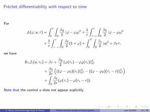
Frechet differentiability with respect to time
For
Jr (ϕ, u, τ) =
∫ τ
0
∫Ω
βQ2|ϕ− ϕQ |2 +
1
r
∫ τ
τ−r
∫Ω
βΩ
2|ϕ− ϕΩ|2
+1
r
∫ τ
τ−r
∫Ω
βS2
(1 + ϕ) +
∫ T
0
∫Ω
βu2|u|2 + βT τ,
we have
DτJr (u, τ∗) = βT +βQ2‖ϕ(τ∗)− ϕQ(τ∗)‖2
L2
+βΩ
2r
(‖(ϕ− ϕΩ)(τ∗)‖2
L2 − ‖(ϕ− ϕΩ)(τ∗ − r)‖2L2
)+
∫Ω
βS2r
(ϕ(τ∗)− ϕ(τ∗ − r)).
Note that the control u does not appear explicitly.
E. Rocca (Universita degli Studi di Pavia) Diffuse interface models of tumor growth June 28,2018 21 / 46
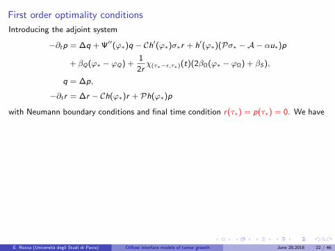
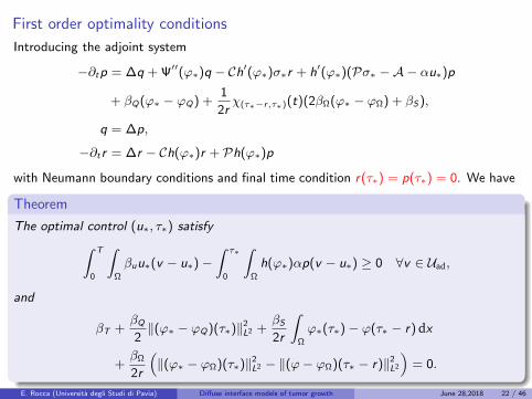
First order optimality conditions
Introducing the adjoint system
−∂tp = ∆q + Ψ′′(ϕ∗)q − Ch′(ϕ∗)σ∗r + h′(ϕ∗)(Pσ∗ −A− αu∗)p
+ βQ(ϕ∗ − ϕQ) +1
2rχ(τ∗−r,τ∗)(t)(2βΩ(ϕ∗ − ϕΩ) + βS),
q = ∆p,
−∂tr = ∆r − Ch(ϕ∗)r + Ph(ϕ∗)p
with Neumann boundary conditions and final time condition r(τ∗) = p(τ∗) = 0. We have
Theorem
The optimal control (u∗, τ∗) satisfy∫ T
0
∫Ω
βuu∗(v − u∗)−∫ τ∗
0
∫Ω
h(ϕ∗)αp(v − u∗) ≥ 0 ∀v ∈ Uad,
and
βT +βQ2‖(ϕ∗ − ϕQ)(τ∗)‖2
L2 +βS2r
∫Ω
ϕ∗(τ∗)− ϕ(τ∗ − r) dx
+βΩ
2r
(‖(ϕ∗ − ϕΩ)(τ∗)‖2
L2 − ‖(ϕ− ϕΩ)(τ∗ − r)‖2L2
)= 0.
E. Rocca (Universita degli Studi di Pavia) Diffuse interface models of tumor growth June 28,2018 22 / 46

First order optimality conditions
Introducing the adjoint system
−∂tp = ∆q + Ψ′′(ϕ∗)q − Ch′(ϕ∗)σ∗r + h′(ϕ∗)(Pσ∗ −A− αu∗)p
+ βQ(ϕ∗ − ϕQ) +1
2rχ(τ∗−r,τ∗)(t)(2βΩ(ϕ∗ − ϕΩ) + βS),
q = ∆p,
−∂tr = ∆r − Ch(ϕ∗)r + Ph(ϕ∗)p
with Neumann boundary conditions and final time condition r(τ∗) = p(τ∗) = 0. We have
Theorem
There exists a unique (p, q, r) to the adjoint system such that
p ∈ L2(0, τ∗;H2) ∩ H1(0, τ∗; (H2)∗) ∩ L∞(0, τ∗; L
2) ∩ C 0([0, τ∗]; L2),
q ∈ L2(0, τ∗; L2),
r ∈ L2(0, τ∗;H2) ∩ L∞(0, τ∗;H
1) ∩ H1(0, τ∗; L2) ∩ C 0([0, τ∗]; L
2).
Theorem
The optimal control (u∗, τ∗) satisfy∫ T
0
∫Ω
βuu∗(v − u∗)−∫ τ∗
0
∫Ω
h(ϕ∗)αp(v − u∗) ≥ 0 ∀v ∈ Uad,
and
βT +βQ2‖(ϕ∗ − ϕQ)(τ∗)‖2
L2 +βS2r
∫Ω
ϕ∗(τ∗)− ϕ(τ∗ − r) dx
+βΩ
2r
(‖(ϕ∗ − ϕΩ)(τ∗)‖2
L2 − ‖(ϕ− ϕΩ)(τ∗ − r)‖2L2
)= 0.
E. Rocca (Universita degli Studi di Pavia) Diffuse interface models of tumor growth June 28,2018 22 / 46
First order optimality conditions
Introducing the adjoint system
−∂tp = ∆q + Ψ′′(ϕ∗)q − Ch′(ϕ∗)σ∗r + h′(ϕ∗)(Pσ∗ −A− αu∗)p
+ βQ(ϕ∗ − ϕQ) +1
2rχ(τ∗−r,τ∗)(t)(2βΩ(ϕ∗ − ϕΩ) + βS),
q = ∆p,
−∂tr = ∆r − Ch(ϕ∗)r + Ph(ϕ∗)p
with Neumann boundary conditions and final time condition r(τ∗) = p(τ∗) = 0. We have
Theorem
The optimal control (u∗, τ∗) satisfy∫ T
0
∫Ω
βuu∗(v − u∗)−∫ τ∗
0
∫Ω
h(ϕ∗)αp(v − u∗) ≥ 0 ∀v ∈ Uad,
and
βT +βQ2‖(ϕ∗ − ϕQ)(τ∗)‖2
L2 +βS2r
∫Ω
ϕ∗(τ∗)− ϕ(τ∗ − r) dx
+βΩ
2r
(‖(ϕ∗ − ϕΩ)(τ∗)‖2
L2 − ‖(ϕ− ϕΩ)(τ∗ − r)‖2L2
)= 0.
E. Rocca (Universita degli Studi di Pavia) Diffuse interface models of tumor growth June 28,2018 22 / 46

Issues with the original functional
To deal with the original functional:
J(ϕ, u, τ) =
∫ τ
0
∫Ω
βQ2|ϕ− ϕQ |2 +
∫Ω
βΩ
2|ϕ(τ)− ϕΩ|2 +
∫ τ
0
∫Ω
βu2|u|2 + βT τ.
Then, the optimality condition for τ∗ is
0 = DτJ |(u∗,τ∗) =
∫Ω
βQ2|(ϕ∗ − ϕQ)(τ∗)|2 +
βΩ
2(ϕ∗(τ∗)− ϕΩ)∂tϕ∗(τ∗) +
βu2|u∗(τ∗)|2 dx
+ βT .
Issues: For the above expression to be well-defined, we need
∂ttϕ∗ ∈ L2(0,T ; L2), u∗ ∈ H1(0,T ; L2).
If we define Uad = u ∈ H1(0,T ; L2) : 0 ≤ u ≤ 1, ‖∂tu‖L2(Q) ≤ K for fixed K > 0, and
impose ϕ0 ∈ H5, σ0 ∈ H3, then we get ϕ ∈ H2(0,T ; L2) ∩W 1,∞(0,T ;H1).
However, to require the a-priori boundedness of ∂tu is difficult to verify in applications.
E. Rocca (Universita degli Studi di Pavia) Diffuse interface models of tumor growth June 28,2018 23 / 46
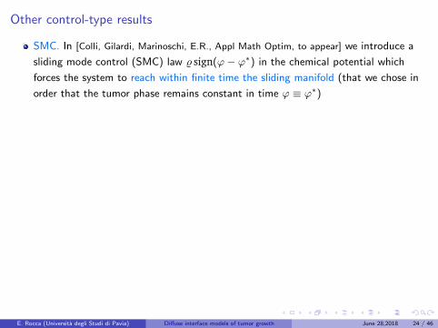
Other control-type results
SMC. In [Colli, Gilardi, Marinoschi, E.R., Appl Math Optim, to appear] we introduce a
sliding mode control (SMC) law % sign(ϕ− ϕ∗) in the chemical potential which
forces the system to reach within finite time the sliding manifold (that we chose in
order that the tumor phase remains constant in time ϕ ≡ ϕ∗)
Different sources. In the phase field model we introduced
∂tϕ = ∆µ+M,
µ = Ψ′(ϕ)−∆ϕ
∂tσ = ∆σ − S + u,
we can choose different form of M and S: linear phenomenological laws for
chemical reactions cf. [Hawkins–Daarud, Prudhomme, van der Zee, Oden (2012)],
[Frigeri, Grasselli, E.R. (2015)]:
M = S = h(ϕ)(σ − µ)
In [Colli, Gilardi, E.R., Sprekels, Nonlinearity (2017)]: the optimal control with respect
to the drug distribution which acts as a control u in the nutrient equation
E. Rocca (Universita degli Studi di Pavia) Diffuse interface models of tumor growth June 28,2018 24 / 46

Outline
1 Phase field models for tumor growth
2 The optimal control problem
3 First order optimality conditions
4 Some simulations
5 A multispecies model with velocity
6 Perspectives and Open problems
E. Rocca (Universita degli Studi di Pavia) Diffuse interface models of tumor growth June 28,2018 25 / 46
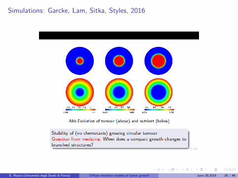
Simulations: Garcke, Lam, Sitka, Styles, 2016
E. Rocca (Universita degli Studi di Pavia) Diffuse interface models of tumor growth June 28,2018 26 / 46

Simulations: Garcke, Lam, Sitka, Styles, 2016
E. Rocca (Universita degli Studi di Pavia) Diffuse interface models of tumor growth June 28,2018 27 / 46

Outline
1 Phase field models for tumor growth
2 The optimal control problem
3 First order optimality conditions
4 Some simulations
5 A multispecies model with velocity
6 Perspectives and Open problems
E. Rocca (Universita degli Studi di Pavia) Diffuse interface models of tumor growth June 28,2018 28 / 46

FLRS: A multispecies model with velocities - with Frigeri, Lam, Schimperna
Typical structure of tumors grown in vitro:
Figure: Zhang et al. Integr. Biol., 2012, 4, 1072–1080. Scale bar 100µm = 0:1mm
A continuum thermodynamically consistent model is introduced with the ansatz:
sharp interfaces are replaced by narrow transition layers arising due to adhesive forces
among the cell species: a diffuse interface separates tumor and healthy cell regions
proliferating and dead tumor cells and healthy cells are present, along with a
nutrient (e.g. glucose or oxigene)
tumor cells are regarded as inertia-less fluids: include the velocity - satisfying a
Darcy type law with Korteveg term
E. Rocca (Universita degli Studi di Pavia) Diffuse interface models of tumor growth June 28,2018 29 / 46

S. Frigeri, K.-F. Lam, E. R., G. Schimperna, arXiv:1709.01469 (2017)
The model is a variant of the one introduced in [Y. Chen, S.M. Wise, V.B. Shenoy and
J.S. Lowengrub, Int. J. Numer. Meth. Biomed. Engng. (2014)]:
ϕp, ϕd , ϕh ∈ [0, 1]: the volume fractions of the cells:
I ϕp : proliferating tumor cell fraction
I ϕd : dead tumor cell fraction
I ϕh: healthy cell fraction
The variables above are naturally constrained by the relation ϕp + ϕd + ϕh = 1
hence it suffices to track the evolution of ϕp and ϕd and the vector ϕ := (ϕp, ϕd)>
lies in the simplex ∆ := y ∈ R2 : 0 ≤ y1, y2, y1 + y2 ≤ 1 ⊂ R2
n: the nutrient concentration (it was σ before)
u:=ui , i = 1, 2, 3: the tissue velocity field. We treat the tumor and host cells as
inertial-less fluids and assume that the cells are tightly packed and they march
together
q: the cell-to-cell pressure
E. Rocca (Universita degli Studi di Pavia) Diffuse interface models of tumor growth June 28,2018 30 / 46

FLRS: the balance law
Letting Ji , i ∈ p, d , h, denote the mass fluxes for the cells, then the general balance
law for the volume fractions reads as
∂tϕi + div(ϕiu) = −divJi + Si for i ∈ p, d , h
where we set Sh = 0, whereas Sp, Sd may depend on n, ϕp and ϕd
Assume: the tumor growth process tends to evolve towards (local) minima of the free
energy functional of Ginzburg–Landau type:
E(ϕp, ϕd) :=
∫Ω
F (ϕp, ϕd) +1
2|∇ϕp|2 +
1
2|∇ϕd |2 dx
where F = F0 + F1 is a multi-well configuration potential, e.g.
F0(ϕp, ϕd):= ϕp logϕp + ϕd logϕd + (1− ϕp − ϕd) log(1− ϕp − ϕd)
F1(ϕp, ϕd) :=χ
2(ϕd(1− ϕd) + ϕp(1− ϕp) + (1− ϕd − ϕp)(ϕd + ϕp))
The fluxes Ji are defined as follows:
Ji = −Mi∇µi , µi :=δE
δϕi= −∆ϕi + F,ϕi for i = p, d
E. Rocca (Universita degli Studi di Pavia) Diffuse interface models of tumor growth June 28,2018 31 / 46

FLRS: the velocity and nutrient evolutions
We set Jh = −Jp − Jd , then upon summing up the three mass balances for i = p, d , h,
using the fact that ϕp + ϕd + ϕh = 1 and Sh = 0, we deduce the following relation:
div u = Sp + Sd =: St
The velocity field u is assumed to fulfill Darcy’s law:
u = −∇q − ϕp∇µp − ϕd∇µd
where q denotes the cell-to-cell pressure and the subsequent two terms have the meaning
of Korteweg forces
Since the time scale of nutrient diffusion is much faster (minutes) than the rate of cell
proliferation (days), the nutrient is assumed to evolve quasi-statically:
0 = −∆n + ϕpn
where ϕpn models consumption by the proliferating tumor cells
E. Rocca (Universita degli Studi di Pavia) Diffuse interface models of tumor growth June 28,2018 32 / 46
The goal and the main difficulties of FLRS
Goal: to study this multispecies model including different mobilities, singular potential
and non-Dirichlet b.c.s on the chemical potential. The main problems are:
we have two different Cahn-Hilliard equations with non-zero right hand sides:
∂tϕi − div(Mi∇µi −ϕiu) = Si and if we do not choose the Dirichlet b.c.s on µi then
we need to estimate the mean values of µi = −∆ϕi + F,ϕi containing a multiwell
logarithmic type potential F0
we need the mean values of ϕi (the proliferating and dead cells phases) to be away
from the potential bareers =⇒ ad hoc estimate based on ODEs technique
indeed, integrating the equations for ϕp and ϕd we obtain an evolution law for the
mean values yi := 1|Ω|
∫Ωϕi dx for i = p, d
such a relation does not involve directly the singular part F0. Hence, the evolution of
yp, yd are not automatically compatible with the physical constraint and this has to
be proved by assuming proper conditions on coefficients and making a careful choice
of the boundary conditions
the choice (Mi∇µi − ϕiu) · n = 0 seems essential
E. Rocca (Universita degli Studi di Pavia) Diffuse interface models of tumor growth June 28,2018 33 / 46

FLRS: The weak notion of solution
Definition. (ϕp , ϕd , u, q, n) is a weak solution to the problem in (0,T )× Ω if the previous
equations hold, for a.e. t ∈ (0,T ) and for i = p, d , in the following weak sense:
〈∂tϕi , ζ〉+
∫ΩMi∇µi · ∇ζ − ϕiu · ∇ζ dx =
∫ΩSiζ dx ∀ζ ∈ H1(Ω),∫
Ωµiζ dx =
∫Ω∇ϕi · ∇ζ + ηiζ + F1,ϕi
(ϕp , ϕd )ζ dx ∀ζ ∈ H1(Ω),∫Ω
u · ∇ξ dx = −∫
Ω(Sp + Sd )ξ dx ∀ξ ∈ H1
0 (Ω),∫Ω
u · ζ dx =
∫Ω−∇q · ζ − ϕp∇µp · ζ − ϕd∇µd · ζ dx ∀ζ ∈ (L2(Ω))d ,
0 = −∆n + ϕpn a.e. in Ω,
ηi = F0,ϕi(ϕp , ϕd ) a.e. in Ω,
Sp = Σp(n, ϕp , ϕd ) + mppϕp + mpdϕd a.e. in Ω,
Sd = Σd (n, ϕp , ϕd ) + mdpϕp + mddϕd a.e. in Ω.
Moreover, there hold the initial conditions
ϕp(x , 0) = ϕp,0(x), ϕd (x , 0) = ϕd,0(x) a.e. in Ω,
where 〈·, ·〉 denotes the duality pairing between H1(Ω) and its dual H1(Ω)′.
E. Rocca (Universita degli Studi di Pavia) Diffuse interface models of tumor growth June 28,2018 34 / 46

FLRS: Assumptions on the mass sources and on the initial data
Set Σ(n, ϕp, ϕd) := (Σp,Σd) and M = (mij), i , j ∈ p, d, the matrix of the coefficients
of the mass souces in the Cahn-Hilliard equations: (Sp, Sd) = Σ + M(ϕp, ϕd)T
Assumption on the mass sources:
Σ is globally Lipschitz and
that there exist a closed and sufficiently regular subset ∆0 contained in the open
simplex ∆ and constants Kp,−,Kp,+,Kd,−,Kd,+ ∈ R, with Kp,− ≤ Kp,+ and
Kd,− ≤ Kd,+, such that Σ(R3) ⊂ [Kp,−,Kp,+]× [Kd,−,Kd,+]
for any x = (xp, xd) ∈ [Kp,−,Kp,+]× [Kd,−,Kd,+], there holds
(My + x) · n < 0 for all y ∈ ∂∆0,
where n denotes the outer unit normal vector to ∆0
Assumptions on the initial data :
ϕp,0, ϕd,0 ∈ H1(Ω) with 0 ≤ ϕp,0, 0 ≤ ϕd,0, ϕp,0 + ϕd,0 ≤ 1 a.e. in Ω,
the mean values satisfy ( 1|Ω|
∫Ωϕp,0(x) dx , 1
|Ω|
∫Ωϕd,0(x) dx) ∈ int ∆0 and
F0(ϕp,0, ϕd,0) ∈ L1(Ω)
E. Rocca (Universita degli Studi di Pavia) Diffuse interface models of tumor growth June 28,2018 35 / 46

FLRS: Examples of mass sources
Examples of mass sources in ∂tϕi − div(Mi∇µi − ϕiu) = Si for i ∈ p, d complying
with the assumptions in the “logarithmic” case are:
Sp = λMg(n)−λAϕp
Sd = λAϕp−λLϕd
for positive constants λM , λA, λL (with λM(λA + λL) < λAλL, λA < 2λL) and a bounded
positive function g such that 0 < g(s) ≤ 1, e.g., g(s) = max(nc ,min(s, 1)) for some
constant nc ∈ (0, 1).
The biological effects we want to model are:
the growth of the proliferating tumor cells due to nutrient consumption at a
constant rate λM
the death of proliferating tumor cells at a constant rate λA, which leads to a source
term for the necrotic cells
the lysing/disintegration of necrotic cells at a constant rate λL
E. Rocca (Universita degli Studi di Pavia) Diffuse interface models of tumor growth June 28,2018 36 / 46

FLRS: Examples of mass sources
Examples of mass sources in ∂tϕi − div(Mi∇µi − ϕiu) = Si for i ∈ p, d complying
with the assumptions in the “logarithmic” case are:
Sp = λMg(n)−λAϕp
Sd = λAϕp−λLϕd
for positive constants λM , λA, λL (with λM(λA + λL) < λAλL, λA < 2λL) and a bounded
positive function g such that 0 < g(s) ≤ 1, e.g., g(s) = max(nc ,min(s, 1)) for some
constant nc ∈ (0, 1). The biological effects we want to model are:
the growth of the proliferating tumor cells due to nutrient consumption at a
constant rate λM
the death of proliferating tumor cells at a constant rate λA, which leads to a source
term for the necrotic cells
the lysing/disintegration of necrotic cells at a constant rate λL
E. Rocca (Universita degli Studi di Pavia) Diffuse interface models of tumor growth June 28,2018 36 / 46

FLRS: Existence of weak solutions
The main result of S. Frigeri, K.-F. Lam, E. R., G. Schimperna, arXiv:1709.01469 (2017)
Theorem
For every T > 0 here exists at least one weak solution (ϕp, µp, ηp, ϕd , µd , ηd , u, q, n) to
the multi-species tumor model on [0,T ] with the regularity
ϕi ∈ H1(0,T ;H1(Ω)′) ∩ L∞(0,T ;H1(Ω)) ∩ L2(0,T ;H2(Ω)),
with 0 ≤ ϕi ≤ 1, ϕp + ϕd ≤ 1 a.e. in Q, for i = p, d ,
µi ∈ L2(0,T ;H1(Ω)), ηi ∈ L2(Q),
u ∈ L2(Q) with div u ∈ L2(Q), q ∈ L2(0,T ;H10 (Ω)),
n ∈ (1 + L2(0,T ;H2(Ω) ∩ H10 (Ω))), 0 ≤ n ≤ 1 a.e. in Q.
Notice that the boundary conditions:
(Mi∇µi − ϕiu) · n = 0, ∂nϕi = 0, q = 0, n = 1 on Γ
are incorporated in the definition of weak solutions
E. Rocca (Universita degli Studi di Pavia) Diffuse interface models of tumor growth June 28,2018 37 / 46
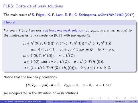
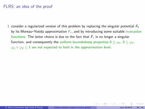
FLRS: an idea of the proof
1 consider a regularized version of this problem by replacing the singular potential F0
by its Moreau–Yosida approximation Fε, and by introducing some suitable truncation
functions. The latter choice is due to the fact that Fε is no longer a singular
function, and consequently the uniform boundedness properties 0 ≤ ϕp, 0 ≤ ϕd ,
ϕp + ϕd ≤ 1 are not expected to hold in the approximation level.
2 to prove existence of a solution to the regularized system a further regularization and
a Schauder fixed point argument: only exploits elementary existence and uniqueness
results methods for PDEs
3 derive the bounds - independent of the regularization parameters - in order to pass
to the limit in the approximation scheme via compactness tools: the main problem is
to bound the mean values of ϕi away from the potential bareers
E. Rocca (Universita degli Studi di Pavia) Diffuse interface models of tumor growth June 28,2018 38 / 46
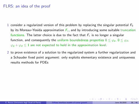

The bound of the mean values
Denoting y(t) := ((ϕp)Ω(t), (ϕd)Ω(t)), (Σ)Ω = ((Σp)Ω, (Σd)Ω), then by testing by 1 the
mass balances
〈∂tϕi , ζ〉+
∫Ω
Mi∇µi · ∇ζ − ϕiu · ∇ζ dx =
∫Ω
Siζ dx ,
where (Sp, Sd) = (Σp,Σd) + M(ϕp, ϕd)T , leads to the following system of ODE’s:
d
dty(t) = (Σ)Ω(t) + My(t) ∀t ∈ [0,T ].
Using the assumption
(My + x) · n < 0 for all y ∈ ∂∆0
we infer that the vector y(t) = ((ϕp)Ω(t), (ϕd)Ω(t)) ∈ int ∆0 for all t ∈ [0,T ]. Indeed, at
the time t = 0, y(0) ∈ int ∆0 by assumption. Suppose that ∃ t∗ such that y(t∗) ∈ ∂∆0.
Taking t = t∗ in the ODE, multiplying with n, we get
d
dty(t∗) · n < 0.
Hence y(t) cannot leave ∆0 and so there exist positive constants 0 < c1 < c2 < 1:
c1 ≤ (ϕp)Ω(t), (ϕd)Ω(t) ≤ c2, c1 ≤ (ϕp + ϕd)Ω(t) ≤ c2 ∀t ∈ [0,T ].
E. Rocca (Universita degli Studi di Pavia) Diffuse interface models of tumor growth June 28,2018 39 / 46

The bound of the mean values
Denoting y(t) := ((ϕp)Ω(t), (ϕd)Ω(t)), (Σ)Ω = ((Σp)Ω, (Σd)Ω), then by testing by 1 the
mass balances
〈∂tϕi , ζ〉+
∫Ω
Mi∇µi · ∇ζ − ϕiu · ∇ζ dx =
∫Ω
Siζ dx ,
where (Sp, Sd) = (Σp,Σd) + M(ϕp, ϕd)T , leads to the following system of ODE’s:
d
dty(t) = (Σ)Ω(t) + My(t) ∀t ∈ [0,T ].
Using the assumption
(My + x) · n < 0 for all y ∈ ∂∆0
we infer that the vector y(t) = ((ϕp)Ω(t), (ϕd)Ω(t)) ∈ int ∆0 for all t ∈ [0,T ].
Indeed, at
the time t = 0, y(0) ∈ int ∆0 by assumption. Suppose that ∃ t∗ such that y(t∗) ∈ ∂∆0.
Taking t = t∗ in the ODE, multiplying with n, we get
d
dty(t∗) · n < 0.
Hence y(t) cannot leave ∆0 and so there exist positive constants 0 < c1 < c2 < 1:
c1 ≤ (ϕp)Ω(t), (ϕd)Ω(t) ≤ c2, c1 ≤ (ϕp + ϕd)Ω(t) ≤ c2 ∀t ∈ [0,T ].
E. Rocca (Universita degli Studi di Pavia) Diffuse interface models of tumor growth June 28,2018 39 / 46

The bound of the mean values
Denoting y(t) := ((ϕp)Ω(t), (ϕd)Ω(t)), (Σ)Ω = ((Σp)Ω, (Σd)Ω), then by testing by 1 the
mass balances
〈∂tϕi , ζ〉+
∫Ω
Mi∇µi · ∇ζ − ϕiu · ∇ζ dx =
∫Ω
Siζ dx ,
where (Sp, Sd) = (Σp,Σd) + M(ϕp, ϕd)T , leads to the following system of ODE’s:
d
dty(t) = (Σ)Ω(t) + My(t) ∀t ∈ [0,T ].
Using the assumption
(My + x) · n < 0 for all y ∈ ∂∆0
we infer that the vector y(t) = ((ϕp)Ω(t), (ϕd)Ω(t)) ∈ int ∆0 for all t ∈ [0,T ]. Indeed, at
the time t = 0, y(0) ∈ int ∆0 by assumption. Suppose that ∃ t∗ such that y(t∗) ∈ ∂∆0.
Taking t = t∗ in the ODE, multiplying with n, we get
d
dty(t∗) · n < 0.
Hence y(t) cannot leave ∆0 and so there exist positive constants 0 < c1 < c2 < 1:
c1 ≤ (ϕp)Ω(t), (ϕd)Ω(t) ≤ c2, c1 ≤ (ϕp + ϕd)Ω(t) ≤ c2 ∀t ∈ [0,T ].
E. Rocca (Universita degli Studi di Pavia) Diffuse interface models of tumor growth June 28,2018 39 / 46

The bound of the mean values
Denoting y(t) := ((ϕp)Ω(t), (ϕd)Ω(t)), (Σ)Ω = ((Σp)Ω, (Σd)Ω), then by testing by 1 the
mass balances
〈∂tϕi , ζ〉+
∫Ω
Mi∇µi · ∇ζ − ϕiu · ∇ζ dx =
∫Ω
Siζ dx ,
where (Sp, Sd) = (Σp,Σd) + M(ϕp, ϕd)T , leads to the following system of ODE’s:
d
dty(t) = (Σ)Ω(t) + My(t) ∀t ∈ [0,T ].
Using the assumption
(My + x) · n < 0 for all y ∈ ∂∆0
we infer that the vector y(t) = ((ϕp)Ω(t), (ϕd)Ω(t)) ∈ int ∆0 for all t ∈ [0,T ]. Indeed, at
the time t = 0, y(0) ∈ int ∆0 by assumption. Suppose that ∃ t∗ such that y(t∗) ∈ ∂∆0.
Taking t = t∗ in the ODE, multiplying with n, we get
d
dty(t∗) · n < 0.
Hence y(t) cannot leave ∆0 and so there exist positive constants 0 < c1 < c2 < 1:
c1 ≤ (ϕp)Ω(t), (ϕd)Ω(t) ≤ c2, c1 ≤ (ϕp + ϕd)Ω(t) ≤ c2 ∀t ∈ [0,T ].
E. Rocca (Universita degli Studi di Pavia) Diffuse interface models of tumor growth June 28,2018 39 / 46

Outline
1 Phase field models for tumor growth
2 The optimal control problem
3 First order optimality conditions
4 Some simulations
5 A multispecies model with velocity
6 Perspectives and Open problems
E. Rocca (Universita degli Studi di Pavia) Diffuse interface models of tumor growth June 28,2018 40 / 46

Perspectives and Open problems
1. To study the long-time behavior of solutions in terms of attractors and/or
trajectories: in case of two-phase models: we have three projects going on: with C.
Cavaterra and H. Wu (on a model by Oden et al.), with A. Miranville and G.
Schimperna (on a model proposed by H. Garcke et. al.), with A. Giorgini, K.-F.
Lam, and G. Schimperna (on the reduction of this model to the two-phase variant).
2. To add the mechanics in Lagrangean coordinates in the problem: for example
considering the tumor sample as a porous media (ongoing project with P. Krejcı and
J. Sprekels).
3. The study of optimal control: we are studying an optimal control problem for a
prostate model introduced by H. Gomez et al. and proposed to us by G. Lorenzo
and A. Reali (ongoing project with P. Colli and G. Marinoschi).
4. Include a stochastic term in phase-field models for tumor growth representing for
example uncertainty of a therapy or random oscillations of the tumor phase (ongoing
project with C. Orrieri and L. Scarpa).
E. Rocca (Universita degli Studi di Pavia) Diffuse interface models of tumor growth June 28,2018 41 / 46

Many thanks to all of you for the attention!
http://matematica.unipv.it/rocca/
E. Rocca (Universita degli Studi di Pavia) Diffuse interface models of tumor growth June 28,2018 42 / 46

Simulations: Garcke, Lam, Sitka, Styles, 2016
E. Rocca (Universita degli Studi di Pavia) Diffuse interface models of tumor growth June 28,2018 43 / 46

Issues with the well-posedness
The state equations
∂tϕ = ∆µ+ h(ϕ)(Pσ −A− αu),
µ = Ψ′(ϕ)−∆ϕ,
∂tσ = ∆σ − Ch(ϕ)σ.
satisfies the energy identity
ddt
∫Ω
(Ψ(ϕ) +
1
2|∇ϕ|2 +
1
2|σ|2)
︸ ︷︷ ︸=:E
+
∫Ω
(|∇µ|2 + |∇σ|2 + h(ϕ)C |σ|2
)
=
∫Ω
h(ϕ) (Pσ −A− αu)µ.
We can estimate the right-hand side as
δ‖µ‖2L2 +
C
δ(P2‖σ‖2
L2 + . . . ) for some δ > 0,
leading to
E(t) +
∫ t
0
∫Ω
(|∇µ|2 + |∇σ|2
)≤ E(0) +
∫ t
0
∫Ω
(δ |µ|2 + other terms...
).
To apply Poincare inequality to the ‖µ‖L2(L2) on the RHS, we need to estimate the square
of the mean of µ using
µ = Ψ′(ϕ)−∆ϕ.
If |Ψ′(s)| ≤ C(1 + |s|p) for some p, then we have∥∥∥∥ 1
|Ω|
∫Ω
µ
∥∥∥∥2
L2(L2)
≤ C(1 + ‖ϕ‖2p
L2p(L2p)) + other terms ...
But, to control ‖ϕ‖2p
L2p(L2p)in the absence of any a priori estimate, we need p = 1! I.e., Ψ
can only be a quadratic potential [Garcke, L.].
E. Rocca (Universita degli Studi di Pavia) Diffuse interface models of tumor growth June 28,2018 44 / 46

Issues with the well-posedness
If σ is bounded in Q, then∣∣∣∣∫Ω
h(ϕ)(Pσ −A− αu)µ
∣∣∣∣ ≤ C‖µ‖L1
and by the Poincare inequality, we have
‖µ‖L1 ≤ C‖∇µ‖L1 + C
∣∣∣∣ 1
|Ω|
∫Ω
µ
∣∣∣∣ .
Then one obtains
E(t) +
∫ t
0
∫Ω
(|∇µ|2 + |∇σ|2
)≤ E(0) + C
∫ t
0
(δ‖∇µ‖L1 + ‖Ψ′(ϕ)‖L1 + other terms...
).
With an assumption like ∣∣Ψ′(s)∣∣ ≤ C1Ψ(s) + C2,
we obtain a priori estimates for potentials with higher polynomial growth.
E. Rocca (Universita degli Studi di Pavia) Diffuse interface models of tumor growth June 28,2018 45 / 46

Issues with the well-posedness
If σ is bounded in Q, then∣∣∣∣∫Ω
h(ϕ)(Pσ −A− αu)µ
∣∣∣∣ ≤ C‖µ‖L1
and by the Poincare inequality, we have
‖µ‖L1 ≤ C‖∇µ‖L1 + C
∣∣∣∣ 1
|Ω|
∫Ω
µ
∣∣∣∣ .Then one obtains
E(t) +
∫ t
0
∫Ω
(|∇µ|2 + |∇σ|2
)≤ E(0) + C
∫ t
0
(δ‖∇µ‖L1 + ‖Ψ′(ϕ)‖L1 + other terms...
).
With an assumption like ∣∣Ψ′(s)∣∣ ≤ C1Ψ(s) + C2,
we obtain a priori estimates for potentials with higher polynomial growth.
E. Rocca (Universita degli Studi di Pavia) Diffuse interface models of tumor growth June 28,2018 45 / 46

The Schauder argument
Given φ ∈ L2(Q), consider the mapping
M1 : L2(Q)→ L∞(0,T ;H1) ∩ L2(0,T ;H2) ∩ H1(0,T ; L2) ∩ L∞(Q),
φ 7→ σ,
where σ solves
∂tσ = ∆σ − Ch(φ)σ.
Then define the mapping
M2 : L2(Q)→ L∞(0,T ;H2) ∩ L2(0,T ;H3) ∩ H1(0,T ; L2),
φ 7→ ϕ,
where ϕ solves
∂tϕ = ∆µ− h(ϕ)(PM1(φ)−A− αu), µ = Ψ′(ϕ)−∆ϕ.
The solution to the fixed point problem
z = M2(z)
yields a triplet (ϕ, µ, σ) which solves the state equations.
E. Rocca (Universita degli Studi di Pavia) Diffuse interface models of tumor growth June 28,2018 46 / 46

The Schauder argument
Given φ ∈ L2(Q), consider the mapping
M1 : L2(Q)→ L∞(0,T ;H1) ∩ L2(0,T ;H2) ∩ H1(0,T ; L2) ∩ L∞(Q),
φ 7→ σ,
where σ solves
∂tσ = ∆σ − Ch(φ)σ.
Then define the mapping
M2 : L2(Q)→ L∞(0,T ;H2) ∩ L2(0,T ;H3) ∩ H1(0,T ; L2),
φ 7→ ϕ,
where ϕ solves
∂tϕ = ∆µ− h(ϕ)(PM1(φ)−A− αu), µ = Ψ′(ϕ)−∆ϕ.
The solution to the fixed point problem
z = M2(z)
yields a triplet (ϕ, µ, σ) which solves the state equations.E. Rocca (Universita degli Studi di Pavia) Diffuse interface models of tumor growth June 28,2018 46 / 46