DI

SC

US

SI

ON

P

AP

ER

S

ER

IE

S

Forschungsinstitut zur Zukunft der ArbeitInstitute for the Study of Labor

Optimal Commodity Taxation andRedistribution within Households

IZA DP No. 5608

March 2011

Olivier BargainOlivier Donni

Optimal Commodity Taxation and Redistribution within Households

Olivier Bargain University College Dublin, IZA and CHILD

Olivier Donni

Université de Cergy-Pontoise, THEMA and IZA

Discussion Paper No. 5608 March 2011

IZA

P.O. Box 7240 53072 Bonn

Germany

Phone: +49-228-3894-0 Fax: +49-228-3894-180

E-mail: iza@iza.org

Any opinions expressed here are those of the author(s) and not those of IZA. Research published in this series may include views on policy, but the institute itself takes no institutional policy positions. The Institute for the Study of Labor (IZA) in Bonn is a local and virtual international research center and a place of communication between science, politics and business. IZA is an independent nonprofit organization supported by Deutsche Post Foundation. The center is associated with the University of Bonn and offers a stimulating research environment through its international network, workshops and conferences, data service, project support, research visits and doctoral program. IZA engages in (i) original and internationally competitive research in all fields of labor economics, (ii) development of policy concepts, and (iii) dissemination of research results and concepts to the interested public. IZA Discussion Papers often represent preliminary work and are circulated to encourage discussion. Citation of such a paper should account for its provisional character. A revised version may be available directly from the author.

IZA Discussion Paper No. 5608 March 2011

ABSTRACT

Optimal Commodity Taxation and Redistribution within Households

Using a collective model of consumption, we characterize optimal commodity taxes aimed at targeting specific individuals within the household. The main message is that distortionary indirect taxation can circumvent the agency problem of the household. Essentially, taxation should discourage less the consumption of a certain group of goods: those for which the slope of the Engel curves is larger for the targeted person. JEL Classification: D13, D31, D63, H21, H31 Keywords: optimal commodity taxation, targeting, intrahousehold distribution Corresponding author: Olivier Bargain UCD Newman Building Dublin 4 Ireland E-mail: olivier.bargain@ucd.ie

1 Introduction

As is well known, commodity taxation can be used as a redistributive device. In optimal

taxation, Diamond (1975) shows that commodities consumed by the targeted group should

be less discouraged by the tax system. Related approaches are interested in the role of

(marginal) commodity taxation in improving social welfare (Ahmad and Stern, 1984) or

reducing poverty (Makdissi and Wodon, 2002). In the same way, it may be possible

to target speci�c, possibly disadvantaged, individuals within households (e.g., children,

women) by choosing optimally the tax rates of some commodities. Despite evidence

that deprivation a¤ects particular individuals within families (e.g., Haddad and Kanbur,

1990), there is little theoretical foundation of the e¤ect of price distortions on the welfare

of individuals within households.

There exists nonetheless a growing literature on the optimal or marginal taxation of

multi-person households (see the general discussion in Pollak, 2005). In particular, the

model of Apps and Rees (1988), concerned with labor supply decisions, focuses on optimal

(linear) income taxation. Balestrino (2004) makes use of a non-cooperative household

model where public goods (children) generate ine¢ ciencies within the household. Cigno

et al. (2003) examine policies that aim to improve child welfare while Bargain and Donni

(2011) compare the e¤ect of price subsidies and cash transfers on child welfare and child

poverty (following the literature on targeting, cf., Besley and Kanbur, 1988). Cremer

and Pestieau (2001) study the optimal non-linear taxation of bequest using a model with

altruistic parents. A few authors also study marginal tax reforms in a collective framework

(Brett, 1988, and with extension to domestic production and labor supply, Allgood, 2009).

More generally, the recent paper of Kleven et al. (2009) on the optimal taxation of couples

focuses on across-family redistribution, yet provides ample motivations to study the e¤ect

of redistributive taxation within families by use of collective models.

This paper aims to bring the literature forward by studying the intra-household redistrib-

ution operated via optimal commodity taxation. Using a multi-person household model,

1

which corresponds to the collective model or to prior versions where Pareto weights are

constant, we characterize the optimal commodity taxes or subsidies that favor speci�c

individuals in the household in a way which possibly departs from the household�s own

redistributive rules (i.e., there is dissonance, in the terminology of Apps and Rees, 1988).

Essentially, we show that the consumption of the goods for which the slope of the En-

gel curves is larger for the targeted person should be less discouraged. This conclusion

contrasts with that of Diamond (1975). We then examine the robustness of this result

when alternative instruments are available, notably instruments that allow governments

to collect tax revenue without distortion (lump-sum taxation) or to directly a¤ect indi-

vidual resource shares in the household. Given that the two latter types of policies are

rarely available, our results suggest using distortionary indirect taxation to circumvent

the agency problem of the household. Since children, men and women tend to consume

di¤erent products/services, there is ample scope for the implementation of redistributive

policies of that type.

2 The Household Model

2.1 The Model and its Comparative Statics

In this section, we consider a two-person household whereby each member i (i = 1; 2)

is characterized by a monotonic, concave, and twice di¤erentiable utility function ui (xi)

which depends on a n�vector of private goods xi. The n�vector of prices is denoted by

p and household income by Y . To specify household behavior, we assume the following.

A1. The outcome of the decision process is assumed to be Pareto-e¢ cient. The house-

hold optimization program can thus be written:

maxx1;x2

��(p; Y ) � u1 (x1) + (1� ��(p; Y )) � u2 (x2) s.t. (x1 + x2)0p � Y: (P)

The weight �� determines the location of the household along the Pareto frontier; it is

2

supposed to be di¤erentiable with respect to prices and income. Several comments must

be made. Firstly, this framework is completely standard. In particular, the separability

in the household welfare function is accepted by the majority of economists, even if not

without reservations (Gronau, 1988). Secondly, the generalization to more than two

household members is feasible but results are more di¢ cult to interpret. The presence of

a disadvantaged versus an advantaged person in the household is enough for our argument.

Thirdly, this setting is very general. For instance, the household may comprise a single

decision maker (the parent, 1) and a powerless person (the child, 2), so that the household

welfare function is simply the objective function of the benevolent parent while Pareto

weights re�ect her level of altruism vis�à-vis the child (Becker, 1991, Bargain and Donni,

2011).1 The model may also describe the behavior of two adults whose relative bargaining

positions are represented by the Pareto weights. In that case, prices and income are likely

to a¤ect adults�bargaining position, as in the model of Apps and Rees (1988) or the

collective model of Chiappori (1988). These two adults are typically the spouses, but

they may also correspond to the head of household and another decision maker like an

older child (see Dauphin et al., 2011).

The �rst order conditions of the optimization program (P) are:

@ui@xi

= �ip;

for i = 1; 2, where �i = ��=��i is the marginal utility of wealth for member i, with ��

the Lagrange multiplier associated to the budget constraint, ��1 = �� and ��2 = 1 � ��.

Solving �rst order conditions with the budget constraint yields the vectors of individual

and household demands:

xi = xi (p; Y ) , i = 1; 2:

1With this interpretation, it may be acceptable to assume that Pareto weights are independent of

prices and income, which is compatible with early representations of multi-person households such as the

Rotten Kid model (Becker 1974, 1991) or the Consensus model (Samuelson, 1956). See Chiappori and

Donni (2011) for a survey of the multi-person household literature.

3

The optimization program (P) is separable so that the decision process can be decen-

tralized: total income is �rst divided between members according to a sharing rule, then

individual programs are solved as if each individual maximized her own utility subject

to her own share of income. Let vi (p; �i) be member i�s indirect utility function where

�i is her share of income. The latter is the solution to:

max�1;�2

��(p; Y ) � v1 (p; �1) + (1� ��(p; Y )) � v2 (p; �2) s.t. �1 + �2 = Y: (P̄)

The �rst order condition of this program is:

��1@v1@�1

� ��2@v2@�2

= 0; (1)

and determines the intra-household sharing of income. Once this is done, individual

programmes can be written:

maxxiui(xi) subject to p0xi � �i(p; Y ): (Pi)

Hence, individual demands are characterized by the following structure:

xi = �i(p; �i); (2)

where �i (�) is a traditional Marshallian demand function. To simplify notation, let � = �1and Y � � = �2, where � (p; Y ) is the so-called sharing rule.

To determine how the intra-household distribution of resources is a¤ected by taxation,

we calculate the derivatives of the sharing rule with respect to income and prices. First,

we di¤erentiate the condition (1) with respect to Y and, after some manipulations, we

obtain:@�

@Y= ��

02=�2�

+MY ; (3)

with

� = ���01�1+�02�2

�> 0 and MY =

1

�

�@ log ��1@Y

� @ log ��2

@Y

�;

where �i = @vi=@�i and �0i = @

2vi=@�2i . The �rst term on the right-hand-side of expression

(3) tells us that, when bargaining weights are kept constant, an increase in income should

4

bene�t both members, but the share is larger for the individual located on the least curved

portion of her utility function. The second term represents the e¤ect of bargaining weights:

if the (log-)weight of member 1 (relatively to that of member 2) increases with income,

then her share of income will increase as well. Bargain and Donni (2011) show that

the term � corresponds to the derivative of the household marginal rate of substitution,

computed at the equilibrium, between the two persons� allocations (a measure of the

convexity of household preferences regarding allocations �1 and �2). It tends to zero

when the substitution between members� income share in problem (P̄) is perfect (i.e.,

indi¤erence curves are straight lines) and equal to in�nity when the complementarity is

perfect (i.e., indi¤erence curves are right-angled lines). The term � is therefore referred

to as the index of complementarity henceforth.

We can now compute the e¤ect of prices on member 1�s income share. First, from Roy�s

identity, we have:@vi@p

= ��ixi;@2vi@p@�i

= ��0ixi � �i@�ji@�i

:

Introducing these expressions in the derivative of (1) with respect to p, and using (3),

leads to:@�

@p=

�(x1 �R)�

@�

@Yx

�� (Mp � xMY ) (4)

where x = x1 + x2 and

R =1

�

�@�1@�1

� @�2@�2

�and Mp =

1

�

�@ log ��1@p

� @ log ��2

@p

�: (5)

The �rst term (bracket) on the right hand side of expression (4) is the price e¤ect when

bargaining weights remain constant while the second term represents the redistribution

due to the e¤ect of prices on bargaining weights. The latter include the direct e¤ect of

prices on weights and an income e¤ect. The former has two components. First, Bargain

and Donni (2011) show that the term (x1 �R) is the change in member 1�s share of income

resulting from a simultaneous variation in prices and in income that keeps total household

welfare unchanged. Second, the term (@�=@Y )x is a �conventional�income e¤ect: person

5

1�s endowment decreases because the real income of the household is reduced by the rise

in the commodity price.

2.2 Elements of Duality Theory.

Some elements of duality theory will be necessary to interpret the optimal tax rates

we shall obtain. Let ei(p; ui) be the expenditure function of member i (dual to the

indirect utility function vi (p; �i)). The �household�expenditure function e(p;u1; u2) is

then de�ned as follows:

e(p;u1; u2) = e1(p;u1) + e2(p;u2):

This function represents the minimum level of expenditure which is required for household

members to attain levels of utility (u1; u2) when prices are equal to p.2 The Envelop

Theorem then gives:

@e

@p(p;u1; u2) = �c1(p;u1) + �

c2(p;u2)

= �c(p;u1; u2)

where �ci (�) denotes the vector of member i�s compensated demand functions, �c (�) the

vector of household compensated demand functions (that is, the minimum level of goods

necessary to attain levels of utility (u1; u2) for prices equal to p, and

@2e

@p@p0(p;u1; u2) =

@�c

@p0(p;u1; u2) = S (6)

where S is a symmetric, semi-de�nite negative matrix. Let us de�ne �S as the pseudo-

Slutsky matrix of the household:

�S =@x

@p0+@x

@Yx0:

2Other representations of the �collective� expenditure function can be found in the literature. See

Browning and Chiappori (1998) for instance.

6

In the appendix, it is shown that

�S = (S� �RR0) + �R (Mp � xMY )0 (7)

On the right-hand-side, the �rst matrix in brackets is the �unitary� substitution e¤ect

under the assumption that bargaining weights are constant. The second matrix, of rank

one, corresponds to the move along the Pareto frontier due to changes in bargaining

weights (Browning and Chiappori, 1998; Donni, 2006). Importantly, if bargaining weights

are constant, the second matrix is equal to zero so that:

�S = (S� �RR0) (8)

is a symmetric, semi-de�nite negative matrix.

3 Optimal Commodity Taxation

We suppose that the household is representative and the government may use excise taxes

on the goods 1; :::; N to raise a certain amount of required revenue B. We consider two

cases: (a) constant bargaining weights, and (b) variable bargaining weights.

3.1 Constant Bargaining Weights

If bargaining weights are interpreted as altruistic terms (caring, in the sense of Becker,

1991), for instance when 2 is a powerless household member, it is not unreasonable to

suppose that they do not depend on prices and income. Formally we suppose the following:

A2. The bargaining weights are constant, that is, ��i (p; Y ) = ���i , for i = 1; 2.

This assumption simpli�es the whole reasoning. The social planner has a set of tax rates

t as instruments and desire to maximize a social welfare function as follows:

maxt�1v1(q+ t; �) + �2v2(q+ t; Y � �);

7

with �1 + �2 = 1, subject to a revenue constraint

(x1 + x2)0t = B

where q is the set of pre-tax commodity prices (and q = p � t), �i is the social welfare

weight on member i in the planner�s function and B the revenue target. If the social

weights �i coincide with the bargaining weights ��i that characterize the decision process

in the household, the traditional Ramsey rule applies and the derivation of the optimal tax

rates is straightforward. However, this will not necessarily be the case, i.e., there may be

dissonance between the preferences of the household and those of the social planner (Apps

and Rees, 1988). We shall focus on this very case for the intra-household redistributive

is important. The �rst order conditions are:

�1�

�@v1@p0

+@v1@�

@�

@p0

�+�2�

�@v2@p0

� @v2@�

@�

@p0

�= �x0 � t0 @x

@p0;

where ��1 is the price of one unit of social welfare in terms of �scal revenue. Since

@vi@�i

=��

��i;

@vi@p

= ���

��ixi;

it can be rewritten as:

�1

�x01 �

@�1@p0

�+ �2

�x02 �

@�2@p0

�= x0 + t0

@x

@p0

where

�i =��=�

��i =�i, i = 1; 2:

The term �=��, the price of one unit of social welfare in terms of household welfare, is

common to both � coe¢ cients. The ratio of social weight and household weight �i=��i

re�ects the dissonance. Then �1 > �2 if social preferences are relatively more favorable

to member 1 than household preferences are.

The tax policy can be broken down into an e¢ ciency motive and a redistributive motive.

To show this, we use the Slutsky condition (7) and the derivative of the sharing rule (4),

and obtain:

�St = �x+ (�1 � �2)R (9)

8

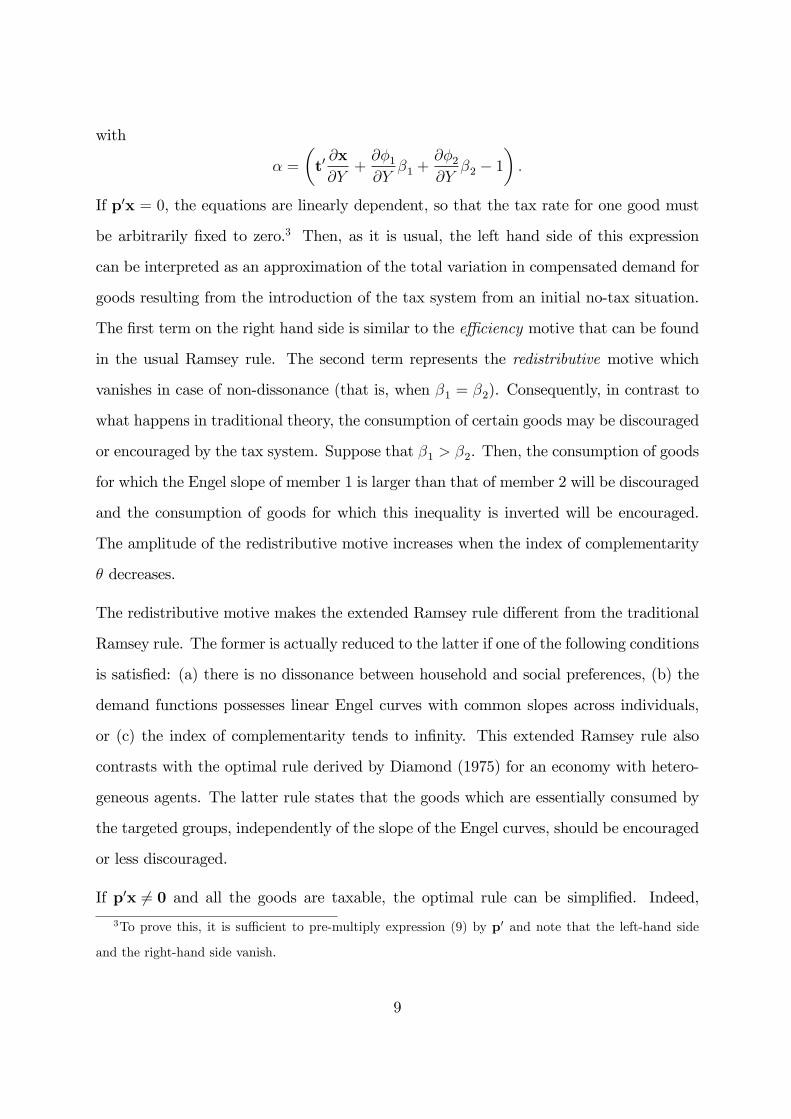
with

� =

�t0@x

@Y+@�1@Y

�1 +@�2@Y

�2 � 1�:

If p0x = 0, the equations are linearly dependent, so that the tax rate for one good must

be arbitrarily �xed to zero.3 Then, as it is usual, the left hand side of this expression

can be interpreted as an approximation of the total variation in compensated demand for

goods resulting from the introduction of the tax system from an initial no-tax situation.

The �rst term on the right hand side is similar to the e¢ ciency motive that can be found

in the usual Ramsey rule. The second term represents the redistributive motive which

vanishes in case of non-dissonance (that is, when �1 = �2). Consequently, in contrast to

what happens in traditional theory, the consumption of certain goods may be discouraged

or encouraged by the tax system. Suppose that �1 > �2. Then, the consumption of goods

for which the Engel slope of member 1 is larger than that of member 2 will be discouraged

and the consumption of goods for which this inequality is inverted will be encouraged.

The amplitude of the redistributive motive increases when the index of complementarity

� decreases.

The redistributive motive makes the extended Ramsey rule di¤erent from the traditional

Ramsey rule. The former is actually reduced to the latter if one of the following conditions

is satis�ed: (a) there is no dissonance between household and social preferences, (b) the

demand functions possesses linear Engel curves with common slopes across individuals,

or (c) the index of complementarity tends to in�nity. This extended Ramsey rule also

contrasts with the optimal rule derived by Diamond (1975) for an economy with hetero-

geneous agents. The latter rule states that the goods which are essentially consumed by

the targeted groups, independently of the slope of the Engel curves, should be encouraged

or less discouraged.

If p0x 6= 0 and all the goods are taxable, the optimal rule can be simpli�ed. Indeed,3To prove this, it is su¢ cient to pre-multiply expression (9) by p0 and note that the left-hand side

and the right-hand side vanish.

9

pre-multiplying expression (9) by p0 and using the homogeneity of demand functions

demonstrate that � = 0. The optimal tax rule then becomes:

�St = (�1 � �2)R: (10)

In particular, a proportional taxation is not optimal unless the right-hand-side of expres-

sion (10) is equal to zero. That is, a proportional tax is optimal if the demand functions

possesses linear Engel curves with common slopes across individuals �this result is remi-

niscent of Deaton (1976) �or if there is no dissonance between the household redistribution

scheme and the social planner�s redistributive objectives.

The interpretation of the optimality rule becomes clearer if commodity j is exclusively

consumed, for example, by member 1. In that case, the rule can be written:Pnk=1 �sjktkxj

= �+ �"j;

where �sjk is a generic element of �S, and

� = � �1 � �2Y (�02=�2)

,

is measure of the redistributive capacity of the tax system, and

"j =Y

xj

@�j1@�1

@�1@Y

!

is the income elasticity of good j; the left-hand-side is the �index of discouragement�in

Mirrless (1976)�s terminology. The level of taxation of an exclusive good is thus related

to the elasticity of its demand with respect to income. In particular, if � > 0, i.e., social

preferences are relatively more favorable to member 1 than household preferences are, and

if the exclusive good j is normal, then its consumption will be relatively encouraged (or

less discouraged) by the tax system.

10

3.2 Varying Pareto Weights

We now extend the previous framework to the case where Pareto weights depend on

post-tax prices and income, i.e., �� = ��(p; Y ).4 In this more general case, the program

(P) corresponds to a collective model with private consumption (Chiappori, 1988). After

some manipulations, the optimal tax rule is now:

(S� �RR0) t = �x+ (�1 � �2)R+ [(�1 � �2) + ] (Mp � xMY ) ; (11)

where = �R0t. The left-hand-side is de�ned by equation (8); it can again be interpreted

as the total variation of the compensated demand functions (on the condition that the

latter are de�ned as the demand functions conditional on the level of total utility and

on bargaining weights). The �rst and second terms on the right-hand-side have a similar

interpretation to that in (9). The third term necessary re�ects the additional redistribu-

tive e¤ects from commodity taxation induced by changes in the bargaining weights. To

interpret it better, suppose that an increase in the price of good j is favorable to the

weight of member 1 (relative to the weight of member 2). That means that Mp�xMY is

positive. If the social planner is relatively more favorable to member 1, i.e., �1 � �2 > 0,

then, all other things being the same, the tax system must encourage the consumption

of good j. However, the tax system also creates distortion at the household level due to

variations in the bargaining weights. In particular, the gain or loss in tax revenue for the

government when one dollar is transferred from member 2 to member 1 via the sharing

rule is represented by . If, for instance, > 0, the empowerment of member 1 increases

tax revenue and the consumption of good j must be all the more encouraged. If < 0,

encouraging the consumption of good j has a cost in terms of tax revenue.

The sign of Mp � xMY can be positive or negative so that it is di¢ cult to draw clear-

cut conclusions. To restrict the dependence of bargaining weights on prices, however, we

follow Browning and Chiappori (1998) and impose some additional structure:4Alternatively, we can also suppose that tax rates enter bargaining weights as speci�c arguments, i.e.,

�� = ��(p; t; y). However, it is di¢ cult to draw strong conclusions at this level of generality.

11

A3. The bargaining weights depend on income de�ated by a linear homogeneous price

index �(p), that is,

��i (p; Y ) = m�i

�Y

�(p)

�:

In other words, the bargaining weights are a¤ected by prices in as much as the prices

in�uence the real income of the household. This re�ects the idea that prices are likely to

have a moderate impact on bargaining weights.5 Then,

Mp � xMY = �@�

@p;

where

� = � Y

��2��@ logm�

1

@ (Y=�(p))� @ logm�

2

@ (Y=�(p))

�:

The optimal rule (11) then becomes:

(S� �RR0) t = �x+ (�1 � �2)R+ [(�1 � �2) + ] �@�

@p: (12)

In addition, some empirical evidence (Haddad and Kanbur, 1994) seems to indicate that

resources are more equally distributed in high-income households than in low-income

households. In that case, a larger Y implies a larger m�1=m

�2, if we assume that 1 is the

disadvantaged person, and � is therefore negative. Then, if the government is supposed to

be favorable to a more equal distribution of resources within the household, the sign of �

must be opposed to that of (�1 � �2), the latter being positive. Neglecting , this implies

that the last term on the right-hand-side of expression (12) is negative and proportional

to @�=@p. Intuitively, if the value of @�=@pj for some good j is particularly large and

positive, the increase in the tax rate on this very good will have a signi�cant e¤ect on the

household real income and, according to the empirical evidence mentioned above, on the

bargaining position of member 1 (relatively to that of member 2) in the household. This

is why the tax placed on good j will tend to be large.

5One exception is wage rates that are known to in�uence bargaining positions in the household.

12

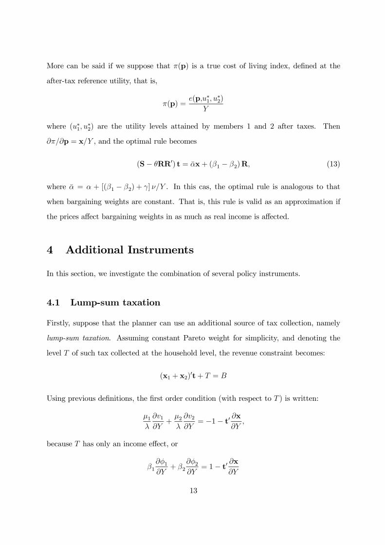
More can be said if we suppose that �(p) is a true cost of living index, de�ned at the

after-tax reference utility, that is,

�(p) =e(p;u�1; u

�2)

Y

where (u�1; u�2) are the utility levels attained by members 1 and 2 after taxes. Then

@�=@p = x=Y , and the optimal rule becomes

(S� �RR0) t = ��x+ (�1 � �2)R; (13)

where �� = � + [(�1 � �2) + ] �=Y . In this cas, the optimal rule is analogous to that

when bargaining weights are constant. That is, this rule is valid as an approximation if

the prices a¤ect bargaining weights in as much as real income is a¤ected.

4 Additional Instruments

In this section, we investigate the combination of several policy instruments.

4.1 Lump-sum taxation

Firstly, suppose that the planner can use an additional source of tax collection, namely

lump-sum taxation. Assuming constant Pareto weight for simplicity, and denoting the

level T of such tax collected at the household level, the revenue constraint becomes:

(x1 + x2)0t+ T = B

Using previous de�nitions, the �rst order condition (with respect to T ) is written:

�1�

@v1@Y

+�2�

@v2@Y

= �1� t0 @x@Y;

because T has only an income e¤ect, or

�1@�1@Y

+ �2@�2@Y

= 1� t0 @x@Y

13

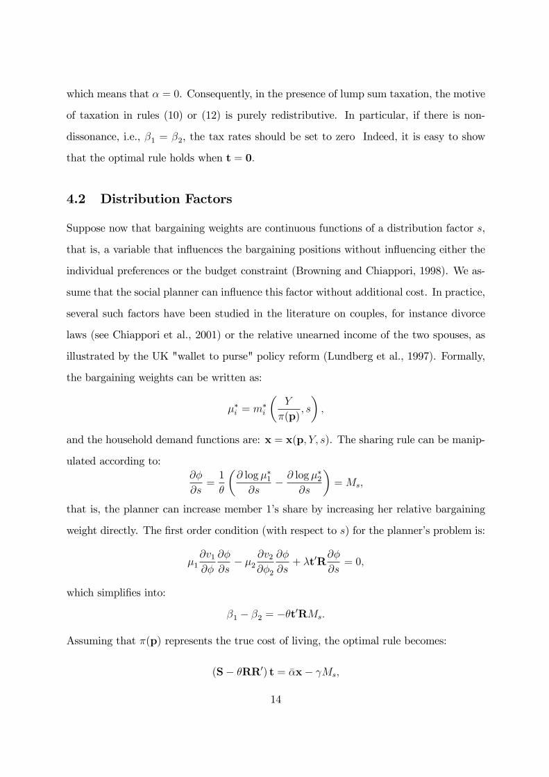
which means that � = 0. Consequently, in the presence of lump sum taxation, the motive

of taxation in rules (10) or (12) is purely redistributive. In particular, if there is non-

dissonance, i.e., �1 = �2, the tax rates should be set to zero Indeed, it is easy to show

that the optimal rule holds when t = 0:

4.2 Distribution Factors

Suppose now that bargaining weights are continuous functions of a distribution factor s,

that is, a variable that in�uences the bargaining positions without in�uencing either the

individual preferences or the budget constraint (Browning and Chiappori, 1998). We as-

sume that the social planner can in�uence this factor without additional cost. In practice,

several such factors have been studied in the literature on couples, for instance divorce

laws (see Chiappori et al., 2001) or the relative unearned income of the two spouses, as

illustrated by the UK "wallet to purse" policy reform (Lundberg et al., 1997). Formally,

the bargaining weights can be written as:

��i = m�i

�Y

�(p); s

�;

and the household demand functions are: x = x(p; Y; s). The sharing rule can be manip-

ulated according to:@�

@s=1

�

�@ log ��1@s

� @ log ��2

@s

�=Ms;

that is, the planner can increase member 1�s share by increasing her relative bargaining

weight directly. The �rst order condition (with respect to s) for the planner�s problem is:

�1@v1@�

@�

@s� �2

@v2@�2

@�

@s+ �t0R

@�

@s= 0;

which simpli�es into:

�1 � �2 = ��t0RMs:

Assuming that �(p) represents the true cost of living, the optimal rule becomes:

(S� �RR0) t = ��x� Ms;

14

where = �t0R is de�ned as previously. Quite surprisingly, the introduction of a dis-

tribution factor, although allowing the government to directly a¤ect the intra-household

distribution of resources, does not allow us to retrieve the traditional Ramsey rule. Indeed,

variations in the distribution factor directly a¤ect the household demand and, thereby,

in�uence the revenue collected by the government. However, if all goods are taxed and

if p0x 6= 0, then a proportional tax will be optimal. This is completely analogous to the

traditional Ramsey rule. To prove this, we suppose that � is a proportional tax and then

show that t = �p solves the system of equation for �� = 0. In that case, the dead weight

loss of the system of taxation is simply equal to zero.

Similarly, if both lump-sum tax and distribution factors are available, a su¢ cient solution

corresponds to setting distribution factors so that dissonance disappears while lump-sum

tax is in charge of revenue collection. Commodity tax is super�uous.

5 Conclusion

Income taxation or transfer to speci�c household members may not achieve its redistrib-

utive goal due to a well-known agency problem: it may be partly or totally neutralized

by the intra-household redistribution process. The main message of our paper is that

distortionary indirect taxation can circumvent the agency problem. That is, it is possi-

ble to operate redistribution in the household via "good" distortions of the price system.

Simply stated, the planner should discourage less the consumption of those goods for

which the slope of the Engel curves of the targeted person is the greater. Since children,

men and women tend to consume di¤erent goods/services, there is ample scope for the

implementation of redistributive policies of that type.

Future work should overcome some of the primary limitations of this contribution, in-

cluding the facts that the analysis is in partial equilibrium and that we account only

for private consumption (it is possible to extend the present model to public goods in

15

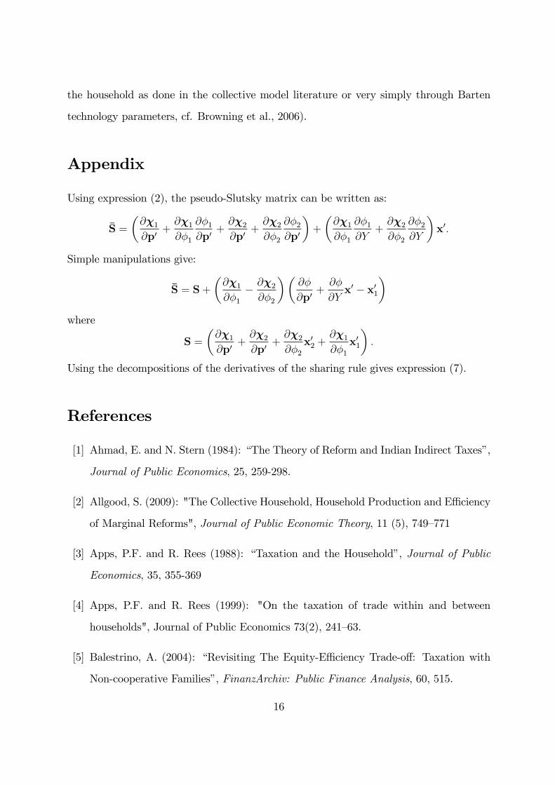
the household as done in the collective model literature or very simply through Barten

technology parameters, cf. Browning et al., 2006).

Appendix

Using expression (2), the pseudo-Slutsky matrix can be written as:

�S =

�@�1@p0

+@�1@�1

@�1@p0

+@�2@p0

+@�2@�2

@�2@p0

�+

�@�1@�1

@�1@Y

+@�2@�2

@�2@Y

�x0:

Simple manipulations give:

�S = S+

�@�1@�1

� @�2@�2

��@�

@p0+@�

@Yx0 � x01

�where

S =

�@�1@p0

+@�2@p0

+@�2@�2

x02 +@�1@�1

x01

�:

Using the decompositions of the derivatives of the sharing rule gives expression (7).

References

[1] Ahmad, E. and N. Stern (1984): �The Theory of Reform and Indian Indirect Taxes�,

Journal of Public Economics, 25, 259-298.

[2] Allgood, S. (2009): "The Collective Household, Household Production and E¢ ciency

of Marginal Reforms", Journal of Public Economic Theory, 11 (5), 749�771

[3] Apps, P.F. and R. Rees (1988): �Taxation and the Household�, Journal of Public

Economics, 35, 355-369

[4] Apps, P.F. and R. Rees (1999): "On the taxation of trade within and between

households", Journal of Public Economics 73(2), 241�63.

[5] Balestrino, A. (2004): �Revisiting The Equity-E¢ ciency Trade-o¤: Taxation with

Non-cooperative Families�, FinanzArchiv: Public Finance Analysis, 60, 515.

16

[6] Bargain, O. and O. Donni (2011): �Targeting and Child Poverty�, in revision for

Social Choice and Welfare

[7] Becker, G.S. (1991): A Treatise on the Family, Enl. Edition, Cambridge University

Press.

[8] Besley, T.J. and R. Kanbur (1988): �The Principles of Targeting�, in: Lipton and

ven der Gaag (eds), Including the Poor, World Bank.

[9] Brett, C. (1998): "Tax reform and collective family decision-making", Journal of

Public Economics 70(3), 425�440

[10] Browning, M. and P.-A. Chiappori (1998): �E¢ cient Intra-household Allocations: A

General Characterization and Empirical Tests�, Econometrica, 66, 1241-1278.

[11] Browning, M., P.A. Chiappori and A. Lewbel (2006): �Estimating Consumption

Economies of Scale, Adult Equivalence Scales, and Household Bargaining Power�,

Boston College Working Paper in Economics 588.

[12] Chiappori, P.-A. (1988): �Rational Household Labor Supply�, Econometrica, 56,

63-89.

[13] Chiappori, P.-A. and O. Donni (2011): �Non-unitary Models of Household Behavior:

A Survey�. In: A. Molina (eds), Household Economic Behaviors, Berlin: Springer.

[14] Dauphin, A., A-R. El Lahga, B. Fortin and G. Lacroix (2011): "Are Children

Decision-Makers Within the Household?", Economic Journal, forthcoming.

[15] Deaton, A. (1979): �Optimally Uniform Commodity Taxes�, Economics Letters, 2,

357-361.

[16] Diamond, P.A. (1975): "A Many-Person Ramsey Rule", Journal of Public Eco-

nomics, 4, 335-42.

17

[17] Donni, O. (2006): �Collective Consumption and Welfare�, Canadian Journal of Eco-

nomics, 39, 124-144.

[18] Donni, O. (2003): "Collective household labor supply: Nonparticipation and income

taxation", Journal of Public Economics 87(5-6), 1179�1198

[19] Gronau, R. (1988): �Consumption technology and the intrafamily distribution of

resources �Adult equivalence scales reexamined�. Journal of Political Economy, 96,

1183�1205.

[20] Haddad, L. and R. Kanbur (1990): �How Serious is the Neglect of Intrahousehold

Inequality?", Economic Journal, 100, 866-881.

[21] Kanbur, R. and L. Haddad (1994): �Are Better O¤ Household More Equal or Un-

equal?�, Oxford Economic Papers, 46, 445-458.

[22] Kleven H.J., C.T. Kreiner and E. Saez (2009): "The optimal income taxation of

couples", Econometrica, 77(2), 537-560.

[23] Lundberg S.J., R.A. Pollak and T.J. Wales (1997): � Do Husbands and Wives Pool

Their Resources? Evidence from the U.K. Child Bene�t�, Journal of Human Re-

sources, 32, 3, 463-480.

[24] Makdissi P. and Q.Wodon (2002): �Consumption Dominance Curves: Testing for

the Impact of Indirect Tax Reforms on Poverty�Economics Letters, 75, 227-235

[25] Mirrlees, J.A. (1976), �Optimal Tax Theory: A Synthesis�, Journal of Public Eco-

nomics, 6, 327-358.

[26] Pollak, R. (2005): "Family Bargaining and Taxes: A Prolegomenon to the Analysis

of Joint Taxation", Taxation and the Family, CESifo Economic Studies, MIT Press.

[27] Samuelson P. (1956): �Social Indi¤erence Curves ", Quarterly Journal of Economics,

70, 1�22.

18