NBER WORKING PAPER SERIES

MAJORITY CHOICE OF TAXATION AND REDISTRIBUTION IN A FEDERATION

Stephen CalabreseDennis Epple

Richard Romano

Working Paper 25099http://www.nber.org/papers/w25099

NATIONAL BUREAU OF ECONOMIC RESEARCH1050 Massachusetts Avenue

Cambridge, MA 02138September 2018

The authors thank Roland Benabou and Thomas Nechyba for his comments. The views expressed herein are those of the authors and do not necessarily reflect the views of the National Bureau of Economic Research.

NBER working papers are circulated for discussion and comment purposes. They have not been peer-reviewed or been subject to the review by the NBER Board of Directors that accompanies official NBER publications.

© 2018 by Stephen Calabrese, Dennis Epple, and Richard Romano. All rights reserved. Short sections of text, not to exceed two paragraphs, may be quoted without explicit permission provided that full credit, including © notice, is given to the source.

Majority Choice of Taxation and Redistribution in a FederationStephen Calabrese, Dennis Epple, and Richard RomanoNBER Working Paper No. 25099September 2018JEL No. H2,H7,H71

ABSTRACT

We provide a model with a federal government and multiple local governments, the former with power to levy an income tax for redistribution, and the latter choosing a local income tax, property tax, lump-sum tax or subsidy, and a local public good. Policy is set by majority choice at each tier of government by households that differ by income and ability to move across communities. We provide sufficient conditions for existence of equilibrium and examine its properties. Central findings are federal income distribution, little local redistribution, and local preference for property taxation over income taxation to fund local public goods.

Stephen CalabreseTepper School of BusinessCarnegie Mellon UniversityPosner Hall, Room 243Pittsburgh, PA 15213sc45@qatar.cmu.edu

Dennis EppleTepper School of BusinessCarnegie Mellon UniversityPosner Hall, Room 257BPittsburgh, PA 15213and NBERepple@cmu.edu

Richard RomanoUniversity of Florida Department of Economics PO Box 117140Gainesville, FL 32611richard.romano@warrington.ufl.edu

1  

1. Introduction

The division of responsibility for redistribution between federal and local governments has been an issue

of longstanding interest within economics. In his submission to the Joint Economic Committee on Federal

Expenditure Policy for Economic Growth and Stability, Stigler (1957) argued that “redistribution is

intrinsically a national policy.” In making his case, he commented that “If 99 communities tax the rich to

aid the poor, the rich may congregate in the hundredth community, so this uncooperative community sets

the tune.” Echoing this theme Musgrave (1971) states “Policies to adjust the distribution of income

among individuals must be conducted on a nationwide basis. Unless such adjustments are very minor,

regional differentiation leads to severe locational inefficiencies. Moreover, regional measures are self-

defeating, as the rich will leave and the poor will move to the more egalitarian-minded jurisdictions.”

Formalizing these ideas in a positive collective choice model has proven elusive. Meltzer and

Richard (1981) develop a positive model with majority choice of redistribution by a national government.

Epple and Romer (1991) develop a positive model with majority choice of redistribution by local

governments in a multi-community setting with mobile households. The challenge of combining these

elements in a single model is compounded by the requirement that a realistic positive model also take

account of the important role of local jurisdictions in providing local public goods. In addition, a positive

model needs to reflect the ability of local governments to choose how much to rely on property versus

income taxation. Combining these elements requires confronting the well-known result (Plott, 1967) that

existence of majority voting equilibrium with multiple policy instruments is problematic, even in a single

jurisdiction. Our goal in this paper is to develop and draw out the implications of a model with majority

choice that embodies all of the elements just enumerated: 1) The model endows national governments

with the authority to tax income and redistribute. 2) The model endows local governments with the

authority to levy property, income, and lump-sum taxes, provide local public goods, and redistribute. 3)

Decisions at both governmental levels are made by majority rule.

More specifically, our model has two tiers of government, a federal government and multiple

local jurisdictions. Policy is determined by majority choice of tax instruments by each government in the

federation. At the federal level, the electorate is the entire population. The federal government can

impose an income tax and use the funds for redistribution. At the local level, eligibility to vote in a

jurisdiction is limited to residents. Each local jurisdiction has purview over a defined geographic area,

with housing supply constrained by the given developable land. The government of each jurisdiction has

access to four policy instruments: property tax, income tax, lump-sum tax or local income subsidy, and

provision of a local (congested) public good. Households are mobile and heterogeneous in incomes.

2  

Of course, despite this array of features, the model does not embody all elements of U.S. governmental

structure. For example, the model has two governmental tiers whereas the U.S. has three. Our goal is to

provide a framework that permits tractable and insightful analysis while avoiding excessive complexity.

We hope that readers will see this balance as being struck judiciously.

We provide conditions sufficient for existence of equilibrium in our theoretical analysis, and we

find those conditions to be satisfied in a quantitative counterpart to our theoretical model. As we noted

above, (Plott, 1967) shows that existence of majority voting equilibrium with multiple policy instruments

is problematic, even in a single jurisdiction. Hence, it may be surprising that existence of majority voting

equilibrium can be established with two independent levels of government, and with multiple local

jurisdictions each of which uses majority rule to choose the values of multiple policy instruments. We

adopt a preference structure that preserves empirically relevant features of the policy environment while

permitting existence and characterization of equilibrium with multiple communities voting over multiple

policy instruments. We view our approach to demonstration of existence to be a key contribution that is

of interest in its own right.

Our analysis provides new insights into the role of household choice of community of residence.

This choice is captured in our model in two ways. Households choose a jurisdiction prior to voting on

local tax-expenditure policies. This gives rise to income stratification. Hence, we refer to this initial

community choice as “sorting.” We also study the effects of potential relocation following voting. We

refer to the latter as “mobility”, and we investigate the effect of varying the proportion of households that

are mobile.1 Thus, our model permits us to examine the differential effects of sorting and mobility, which

we show to be important.

Four key positive implications from our theoretical and quantitative analysis accord well with

features observed in the U.S.2 1) At the federal level, an income tax is adopted to fund income

redistribution. 2) At the local level, there is income stratification across jurisdictions. 3) When use of

lump-sum taxes is constitutionally limited, as observed in practice, localities other than the central city

rely on property taxation to fund provision of local public goods. They eschew use of income taxes, and

they do not redistribute. 4) Within the central city, revenue is raised with property taxes supplemented

with very modest income taxation. This revenue is used to provide local public goods and to provide

some limited income redistribution.

                                                            1 Kessler and Lufesmann (2005) likewise model household locational choice and examine redistribution in a Tiebout model with one tier of government. 2 See Baicker, Clemens, and Singhal (2012) for U.S. evidence regarding federal vs. local public expenditure and taxation policies.

3  

As we noted above, the traditional argument, going back to Stigler (1957) and Musgrave (1971),

is that households’ ability to relocate among local jurisdictions curtails the incentive to attempt local

redistribution; an attempt by the pivotal voter in a community to redistribute would cause richer

households to emigrate and poorer households to immigrate, with dire consequences for the tax base. Our

findings support the prediction that localities will not redistribute, but, interestingly, the mechanism

giving rise to this outcome is somewhat different from that suggested by Stigler and Musgrave. The

mechanism is as follows. Households sort across communities because of differing preferences for local

public goods. This gives rise to income stratification across communities. Median income is typically less

than the mean in communities, seemingly setting the stage for pivotal voters in all communities to tax for

redistribution. However, because of sorting, the difference between median and mean income within

communities is relatively small. In addition, any local taxes for redistribution come atop taxes that fund

the local public good and atop the federal income tax. Such additional local taxes would create an

additional deadweight loss larger than the gain that the pivotal voter would obtain from the redistribution.

Thus, we find that local redistributive taxes would not arise even if voters could not relocate to avoid such

a tax. In short, it is not mobility that precludes local redistribution, rather it is sorting. The sorting effects

and implied differences in voter preferences for redistribution at the federal and local levels also imply

contrasting findings to those of Boadway, Marchand, and Vigneault (1998) and Gordon and Cullen

(2011), discussed below.

We also undertake quantitative comparison of normative properties of equilibrium in federal

systems to cases of one-tiered government. The main results here are: 1) Permitting federal taxation for

redistribution increases equity but reduces efficiency as a result of their redistributive policy; and 2)

Household sorting across localities in a federal system is highly inefficient unless local lump-sum

taxation is unrestricted, this a generalization of the key finding in Calabrese, Epple, and Romano (2012).

As noted, a key theoretical challenge is the “Plott (1967) problem” that arises with majority

choice equilibrium over multiple policy variables. The preference function we adopt permits us to map

preferences over a 6-element policy and price vector into a simple linear indirect utility function over two

“composite public goods.” This greatly simplifies the analysis and provides intuition about relative

policy preference of households with differing incomes. It facilitates proving existence of majority

choice in the local jurisdictions and also facilitates the analysis of household sorting.3 In addition, this

characterization permits development of sufficient conditions for existence of majority choice of the

federal income tax for direct redistribution. This approach may in turn prove valuable in other

applications with multiple policy instruments, discussed in the Conclusion.

                                                            3 This simplification permits us to use single-crossing properties to establish existence results, placing the Plott existence conditions in the background.

4  

This paper bridges two literatures in public finance. The equilibrium among the local

jurisdictions in our model conforms to a Tiebout equilibrium, so this paper relates to the large theoretical

Tiebout (1956) literature on multi-jurisdictional economies with endogenous policy determination.4

Much of this literature is focused on efficiency issues, while our key contribution about existence is

positive. There is limited positive research on multiple tax instruments, surely because of the Plott

existence problem, with the following exceptions. Along the lines of the Plott conditions, Bucovetsky

(1991) provides sufficient restrictions on voters’ utility function that imply existence of majority choice

equilibrium in a single jurisdiction setting with multiple policy instruments. Krelove (1993) examines the

preferred tax form in a multi-jurisdictional model assuming identical households. Henderson (1994) also

studies choice of tax instruments in a multi-jurisdictional setting with identical households, comparing

voting equilibrium to developer equilibrium. The assumption of identical households resolves the

existence problem among voters in the latter two papers. Nechyba (1997) shows in a multi-jurisdictional

model with mobile heterogeneous households that, with availability of both income and property taxes to

finance public goods, only property taxation arises unless jurisdictions collude (or there is another

centralized tier of government). Voting is over just the property tax with community planners (or a

central authority) setting income taxes. The dominance of property taxes absent collusion is due to

household mobility. Our models differ in several ways, including our examination of majority choice in

both tiers of government and of direct redistribution.5 The utility specification used here to establish

existence of majority choice equilibrium is presented in Calabrese, Cassidy, and Epple (2002). We

generalized the latter analysis in Calabrese, Epple, and Romano (2015; CER henceforth). In this paper,

we generalize the CER (2015) model to include a centralized government.6 Adding a central government

is essential for providing a positive analysis of tax and expenditure instruments chosen at different

government levels, for explaining the extent of redistribution that arises in reality, and for analyzing how

local majority choice is affected by the central government. Adding a multi-layered governmental

structure poses new theoretical challenges that we address in this paper. Epple and Romer (1991) show

local redistribution can characterize equilibrium in a single-tiered Tiebout model that assumes local

property taxation, in contrast to our findings. As summarized above and discussed further below, the key

                                                            4 Important references not noted elsewhere are Ellickson (1971), Hamilton (1975), Westhoff (1977), Wooders (1980), Wildasin (1980), Boadway (1982), Brueckner (1983,2004), Zodrow (1984), Epple, Filimon, and romer (1984), Inman (1989), deBartolome (1990), Benabou (1993,1996), Wilson (1997), Nechyba (1999,2000), Fernandez and Rogerson (1996,1998), and Epple and Platt (1998), and Epple and Romano (2003). A strand of the literature concerns taxation of mobile capital which is not an element of our model. 5 Nechyba’s model includes a national public good, which we do not have. Nechyba’s consideration of state income taxation with local property taxation relates to the fiscal federalism literature discussed below.    6 For tractability in the more complex setting here, we use a “utility taking” assumption concerning voter’s beliefs, while a Nash assumption in made in CER (2015). This is explained below.

5  

difference explaining the alternative findings about local redistribution is the existence of local public

goods in our model: Local public good provision increases the distortion from property taxation,

deterring local property taxation to redistribute.7

Another large literature on fiscal federalism concerns the vertical relationship between tiers of

government. Much of the fiscal federalism literature is intended to explain decentralized (local) versus

centralized (federal) provision of public goods, with Oates’ (1972a, 1972b) Decentralization Theorem the

centerpiece.8 Within the fiscal federalism literature, papers most closely related to ours are those that

examine equilibrium choice with two tiers of government. In particular, Boadway, Marchand, and

Vigneault (1998; BMV henceforth) and Gordon and Cullen (2011; GC henceforth) make headway in

modeling redistributive income taxation in two tiered government employing an alternative to majority

decision making.9 BMV and GC both assume the objective of the central government’s decision maker

weighs all households, with an incentive to redistribute wealth, and local government decision makers

have the same form of objective but place weight only on residents in their locality.10 Assuming imperfect

mobility of households between local jurisdictions and some taxation and redistribution by the central

government, the local government decision makers have one incentive to engage in excessive local

redistribution since part of the efficiency costs spill over to other localities through the effects on central

redistribution – a vertical externality - but they (sometimes in BMV) have a counter-incentive to

redistribute too little to attract (repel) wealthier (poorer) households – a horizontal externality. The

central government engenders the efficient allocation by taxing and redistributing so that the vertical

externality localities face offsets the horizontal externality. Then equilibrium has both federal and local

income taxation and redistribution, in sharp contrast to our findings. What underlies the contrasting

                                                            7 Hansen and Kessler (2001) examine mobility, redistribution, and income sorting assuming income taxation with one tier of government and two jurisdictions. If one jurisdiction is sufficiently small, then income stratification results in equilibrium with the rich clustered in the small jurisdiction and very limited redistribution there. The latter finding is akin to the lack of local redistribution we find resulting from sorting. In a very similar model, Rohrs and Stadelmann (2014) show that a sufficiently large immobile population (equated to home owners in their model) supports equilibrium income sorting and local redistribution can arise. Like in Epple and Romer (1991), these models have no local public good. 8 The thrust of the Theorem is that public good provision should be locally determined whenever no externalities outside the locality arise, this to facilitate local preference matching. See Oates (1999) for discussion and references and Nechyba and Epple (2004) for a wider survey and additional references. A second wave of research on centralization v. decentralization begins with the observation that centralized provision can vary across localities, thus expanding the inquiry about the relative advantage of decentralized provision. This strand of the literature shows alternative political regimes can explain whether centralization or decentralization is relatively efficient. See Lockwood (2006) for a survey and references. 9 See also Gordon (1983), Johnson (1988), Wildasin (1991), Inman and Rubinfeld (1996), and Feldstein and Wrobel (1998). 10 For expositional efficiency, our discussion of these two papers suggests the papers are essentially the same, when in fact GC significantly advance the analysis. BMV assumes linear income taxation, while GC examine fully nonlinear taxation. GC use a more general objective function of the government decision makers. GC evaluate their more complete predictions empirically.

6  

findings? While several differences characterize the models (e.g., we consider multiple local tax

instruments), the crucial distinction is our examination of majority choice at each government tier

combined with equilibrium household sorting across local jurisdictions. The effective federal decision

maker in our model, who is the pivotal federal voter, has median income, strong incentive to redistribute,

and then does so. The effective local decision makers, the local pivotal voters, have much weaker

incentives to redistribute as a result of equilibrium income stratification and tax distortions from federal

taxation and local provision of public goods. Their net incentives typically imply no local redistribution.

In the main models of BMV and GC, the federal and local decision makers have the same strong

objective to redistribute, though face different constraints. Equilibrium then has both engage in some

redistribution.

To summarize our contributions, first we show existence of equilibrium for a federation with two

tiers of government and majority choice of tax instruments and redistribution at both tiers. Second, our

model explains how redistribution emerges as the purview of the federal government when there is

majority choice at two tiers of. In particular, we demonstrate that sorting across local jurisdictions is of

first-order importance in driving this division of responsibility across tiers, and we also demonstrate that

this division of responsibility is little affected by the potential for households to relocate after policy is

set. Third, we show a strong preference for not taxing income locally, either to provide local public goods

or to redistribute. Instead, voters prefer relying on property taxation and lump-sum taxes (if allowed).

Finally, we generalize a result (Calabrese, Epple, and Romano, 2012) concerning the inefficiency of

household sorting in Tiebout equilibria that proscribes lump-sum taxation and relies on property taxation.

This paper proceeds as follows. In the next section, we present the model. General theoretical

results are presented in Section 3. The quantitative analysis makes up Section 4, including analysis of

variations in the main model. Section 5 concludes. Some technical analysis is collected in an on-line

appendix.

2. The Model

Here we develop the main federal system model.

2.1 Households. The economy consists of a continuum of households that differ in their endowed income

y and whether they are mobile. The economy pdf of income is denoted f(y), positive on its support

min maxS [y , y ] R . Normalize the economy’s population to equal 1. An exogenous proportion

(y) [0,1] of income y households are mobile, the precise meaning clarified below. Households obtain

utility from consumption of a local public good, g, the quality/quantity of housing consumed, h, and

numeraire consumption, b. Households have the same utility function of form:

7  

(1) U(g,h,b) v(g)u(h,b)

with all functions increasing and twice differentiable, and with u(h,b) quasi-concave and homogeneous of

degree 1.11 While obviously restrictive, (1) permits substantial variation in preferences, and income

affects demands in a realistic way. There is variation in estimates of the income elasticity of housing

demand, but unitary elasticity implied by this specification falls well within the range of empirical

estimates (e.g., Harmon 1988). Higher income households obtain a higher marginal benefit from

increases in the local public good.

2.2 Jurisdictions and Housing Supplies. The economy is divided into an integer number of jurisdictions, J,

each characterized by a non-decreasing housing supply function: j js hH (p ), j 1,2,...J; where j

hp denotes

the supplier price of housing services. Throughout we use a j superscript to indicate a value for

jurisdiction j, though dropping it where obvious by context. The notation ‘ j ’ indicates the set of

jurisdictions other than j. Households rent housing in their local competitive housing market. We assume

housing suppliers are absentee for simplicity. We later show the main results carry over to a case with

housing owners. We frequently refer to a jurisdiction alternatively as a “community.”

2.3 Policy and Timing of Choices. We first give a brief overview of the timing of choices, and then

provide the detail. Equilibrium unfolds in five stages (see Figure 1). In Stage 1, households choose by

majority vote an economy-wide or federal income tax fm 0, the proceeds of which are used for a lump-

sum income transfer, rf. Second, in Stage 2, households select a jurisdiction where they plan to live and

will vote on local policy. Third, in Stage 3, households vote on local policy consisting of a property tax, jt 0; local income tax, jm 0; and local lump-sum transfer (or tax if negative), rj; with net tax revenues

used to provide a local public good, gj. Fourth, in Stage 4, mobile households can costlessly relocate to

another jurisdiction.12 Fifth, in Stage 5, housing is chosen and local housing markets clear, federal and

local budgets balance determining respectively rf and gj, and households consume.

We can now provide a more detailed description, working backward from Stage 5. Entering

Stage 5, the policy vector j j j j fP (m ,t ,r ,m ) in each jurisdiction j is given, where we include the federal

income tax rate in the vector. Each jurisdiction’s measure of income types, denoted fj(y), is also

determined prior to Stage 5. Let j j

Sn f (y)dy denote the “number” of households residing in j. In

Stage 5, the values of individual housing consumption, jdh (y), numeraire consumption, j

db (y), taxable

                                                            11 Our results apply to an extended version of the utility function with U = vꞏ(u+φ), with φ a constant. 12 We use the expression “mobility” here to refer to the ability to move between jurisdictions following initial community choice, in contrast to Epple and Romer (1991) who use mobility to refer to the ability to select a jurisdiction in which to live prior to local policy choices. The present model also assumes the latter “mobility.”

8  

income, jx (y), the gross and net housing prices, j jh(p ,p ), local public good levels, and the federal

transfer are determined, satisfying the following set of equations.

(2) j j

j j j j jd d h ,b

j j j j f f j f j

(h ,b ) ARGMAX v(g )u(h ,b )

s.t. b p h r r y{1 [1 (m m )](m m )}

(3) f j f j

jf j

y {1 [1 (m m )](m m )}x (y) .1 m m

(4) j j j jd s hS

h (y)f (y)dy H (p )

(5) j j jhp (1 t )p

(6) j j j j j j j j js hS

n (r g ) m x (y)f (y)dy t p H (p )

(7) Jf f j j jj 1 S

r m x (y)[f (y) / n ]dy

Equations (2) and (3) describe individual consumption, where ( ) 0 is a non-decreasing and continuous

income tax distortion function. This specification follows Feldstein (1999). Feldstein (1999) shows that

the deadweight loss of tax avoidance through changes in forms of compensation (e.g., provision of health

insurance by employers) and through changes in the patterns of consumption that avoid taxation (e.g.,

leisure consumption) can be evaluated as the deadweight loss of an excise tax on non-deductible

consumption. Total non-deductible consumption is given by housing expenditures (pjhj) plus

consumption of the composite good bj, but subtracting the lump-sum transfers rj +rf that we assume are

not taxed. Thus, the household’s budget constraint is as stated in (2). In turn, taxed income, xj, satisfies

(3). Our subscripts d on the consumption values are to denote Marshallian demand.

Equations (4) is the housing-market clearance condition, with (5) the identity between gross and

net housing price. Equation (6) is the local government budget balance condition. Equation (7) is the

federal government budget balance condition.

With our assumption on the utility function and the housing supply functions, all values

determined in Stage 5 are unique given the input vector (Pj,fj(y)).

In Stage 4, mobile households can costlessly relocate to another community. The 1 (y)

immobile households with income y are locked into the community they choose in Stage 2. We

investigate computationally how varying (y) affects equilibrium. Following the literature on club

goods, we assume mobile households are “utility takers” in making their own relocation choice and in

9  

anticipating relocation choices of others. To clarify this simplifying assumption, note first that no one

relocates in equilibrium as explained below, but relocation can occur off the equilibrium path. Utility

taking means that households in community j take the equilibrium policies and prices in communities

k j as given, and then compute utilities of any mobile households under this assumption in predicting

moving. This is an approximation since this utility would not generally equal the continuation utility if

there is a finite population change in community k.13 Note that households correctly anticipate all

continuation equilibrium values in their initially chosen community given the latter relocations.

Entering Stage 3, initial locations and the federal tax rate are fixed. In each community j,

majority choice of the local policy vector (mj,tj,rj) occurs, with all households anticipating the

continuation values in Stages 4 and 5.

In Stage 2, given mf, households choose their “initial” communities, anticipating how equilibrium

will unfold. Since households are atomistic and thus individually have no effect on policy, mobile

households are actually indifferent to their initial community choice. We then restrict attention to “no-

relocation equilibria,” which assumes mobile households select the community where they will ultimately

reside. As noted above, no household relocates on the equilibrium path. A no-relocation equilibrium is

also the only type of equilibrium if households discover whether they are mobile after having chosen their

initial community.14

In Stage 1, majority choice by all households of the federal income tax occurs, with households

anticipating the resulting equilibrium from Stage 2 forward. In Section 5 we analyze some variations in

the model and discuss further some of our modelling assumptions.

2.4 Existence of Equilibrium, Community Differentiation, and Equilibrium Selection. We do not have a

general existence proof, but develop sufficient conditions for existence that can be checked

computationally. We confirm that these conditions hold in our quantitative analysis. We also

demonstrate in our computational analysis that equilibrium exhibits stratification of households by

income across all jurisdictions. By contrast, in many multi-jurisdictional models where equilibria with

differentiated communities exists, equilibria also exist in which two or more jurisdictions have the same

income distributions and the same policies.15 We do not find such “clone community” equilibria due to

                                                            13 Since P-j is committed before Stage 4, it is the values of g-j and rf that can change following finite relocations and then change utility from the models’ equilibrium utility. Utility taking then means that households do not have fully rational expectations off the equilibrium path. This assumption greatly simplifies computation of equilibrium and some proofs, and we have found it in closely related analysis (e.g., CER, 2015) to have very minor quantitative effects relative to assuming full rationality and subgame perfection. 14 Specifically, then let (y) denote the known probability that a household with income y will be mobile, an individual’s mobility discovered following initial location but before Stage 3 commences. 15 Models where this arises that include housing markets assume that jurisdictional housing supplies are proportional, e.g., the same. This permits equilibrium housing prices to be the same in every jurisdiction.

10  

household mobility. In such equilibria, households anticipate the same populations and policies, and then

are indifferent to where they locate initially, thus are content to sort to have clone communities.

Moreover, with the same community populations, equilibrium policy choices will be the same. However,

provided some households are mobile (i.e., (y) is bounded above 0) and the same local policies and

populations characterize communities, then a marginal policy change in one jurisdiction will induce finite

population relocation. We find that the pivotal voter would generally prefer a small policy change to

induce “massive” desirable household relocations (e.g., increasing the local lump-sum tax to draw in

richer households, while driving out poorer households). With jurisdictions stratified by income,

marginal local policy changes induce marginal relocations so that equilibrium can exist.

Regarding equilibria with income stratification, a multiplicity issue arises if jurisdictional housing

supplies differ. Suppose, for example, that J= 2 and one jurisdiction has rightward shifted housing supply

relative to the other. Any stratified equilibrium has a rich and poor jurisdiction. Two such equilibria can

then arise, one with the “larger” community being the rich one, and the other with the larger community

the poor one. The threshold income separating the two income strata in the two equilibria will generally

differ. More generally, there can be J! alternative stratified equilibria. We resolve this issue by assuming

the largest jurisdiction (i.e., with most rightward shifted housing supply) is the poorest (the central city),

the second largest is the second poorest (poorest suburb), and so on. Thus, when voting in Stage 1 on the

federal income tax rate and when making their initial community choices in Stage 2, households

anticipate among any multiplicity of stratified equilibria the latter type equilibrium. Note, too, that if each

jurisdiction has the same housing supply, this multiplicity issue does not arise.

3. Theoretical Results

3.1 Indirect Utility over Composite Public Goods. The form of the utility function in (1) underlies

existence of equilibrium, especially with regard to existence of majority choice equilibrium over local

policies. Lemma 1 describes an indirect utility function that facilitates showing our main results.

Lemma 1. Indirect utility of household y living in community j is given by:

(8)

j j j j

j j f j f j j

j j f j j

j

V( , , y) y ;v(g ) [1 (1 (m m ))(m m )] w(p );v(g ) (r r ) w(p );

where w (p ) 0.

11  

Lemma 1 is shown by solving the maximization in (2) using the assumed form of utility in (1).16 Lemma

1 is closely related to Proposition 1a in CER (2015).17 A proof is provided in the on-line appendix, which

closely tracks the proof in the latter paper.

The value of Lemma 1 is that for given policies (Pj,gj,rf) and housing price pj, whether set or

anticipated, utility is a simple linear form in the “composite public goods” j j( , ) and income. In

addition, it is implied that higher income households have a relative preference for j, with indifference

curves j jV( , ,y) const. linear if drawn in the j j( , ) plane and satisfying single crossing in income.

Higher income households are willing to give up more j for j at any ( , ); j j the indifference curves

flatten as income rises. As one can see by inspection of (8), higher income households are more averse to

income taxes, while lower income households place a higher relative value on lump-sum positive income

transfers. Note, though, that the converse of the latter observation is that higher income households have

a relative preference for a local lump sum tax (i.e., rj < 0).18 Aversion to property taxes is implied by (5)

and that jw (p ) 0 in (8).19 This simple form of the indirect utility function plays a central role in all the

propositions that follow.

3.2 Jurisdictional Majority Choice Equilibrium. The first proposition regards majority choice

equilibrium of local policies in the J jurisdictions, or the continuation equilibrium of the model at the

beginning of Stage 3. To characterize and understand this continuation equilibrium, define jurisdiction j’s

government budget constraint (GBCj) as the locus of values of j j( , ) as policies (mj,tj,rj) vary over their

feasible values. Along a GBCj, mf is given (pre-determined), and with (gj,pj,rf) satisfying (2)-(6) given

initial locations and anticipated relocations by community j residents that satisfy the utility taking

assumption (determining fj(y)). We write the locus as j j j fGBC ( , ;m ) 0. Figure 2 shows an example

of a GBC.

A voter in jurisdiction j has preferred policy that solves:

(9) j j

j j,

j j j f

MAX y

s.t. GBC ( , ;m ) 0

                                                            16 The indirect utility function is an example of what Grandmont (1978) termed “intermediate preferences.” 17 In CER (2015), there is no federal government, hence no federal income tax and transfer. Lemma 1 generalizes Proposition 1a in CER (2015) to the presence of a federal policy. 18  j is negative if community j has a lump sum tax that is higher than the federal income transfer rf. 19 Aversion to property taxes assumes a non-zero housing supply elasticity so that housing suppliers do not bear the full incidence of a property tax.

12  

The main result here is:

Proposition 1. For any mf, majority choice equilibrium of policy exists in each jurisdiction j, and an

equilibrium policy in jurisdiction j is a preferred policy of the median income household residing there.

Proof of Proposition 1. To make the argument, first assume that when voting every resident of

jurisdiction j does not itself plan to relocate for any policy in jurisdiction j, though anticipating all others’

relocations under the utility taking assumption. Then, using the single-crossing property of the indirect

utility function, a standard argument implies the results in the Proposition regardless of the shape of the

GBC.20 We must argue that this pseudo-equilibrium continues to be the majority choice equilibrium

when mobile voters contemplate their own relocation if optimal. No one household’s relocation choice

affects the GBC, so the GBC is the same as in the pseudo-equilibrium. The pseudo-equilibrium is in fact

an equilibrium, for the following reason. All those in the majority that vote against any alternative policy

to the candidate equilibrium policy in the pseudo-equilibrium would continue to do so allowing them to

move if they prefer. Obviously, any in this majority would continue to vote against an alternative policy

if they would not relocate under the alternative policy. If they would relocate, then they anticipate lower

utility than in the candidate equilibrium. This follows because their initial community choice maximizes

utility among the policies that arise in equilibrium in all communities (by the no-move element of

equilibrium on the equilibrium path). Thus, all in the majority would continue to prefer the candidate

equilibrium policy and vote against the alternative. Thus, the candidate equilibrium policy continues to

garner a majority against all other policies and is therefore an equilibrium.

To complete the proof we must show that only a preferred choice of the median income

household in the community is a majority choice equilibrium. Again, first assuming no voter

contemplates their own moving when voting, the single-crossing property implies a preferred choice of

the median income household is majority preferred to any other feasible policy (on or below the GBC).

But since no one relocates in equilibrium and relocating out of equilibrium implies lower utility than in

equilibrium, the majority preference for a median income household’s preferred policy over any other is

sustained. ▀

Given household sorting and mf, equilibrium in any jurisdiction is generically unique since the

preferred policy of a median income household is generically unique. This follows since the equilibrium

is a tangency between the median income household’s indifference curve and the GBC (see Figure 2), and

multiple tangencies between the GBC and the given indifference curve will not arise generically as the

GBC depends on the entire population of the community.

                                                            20 See, e.g., Epple and Romer (1991). 

13  

While dependent on the assumed form of the utility function, the generality of existence of the

community majority choice equilibrium bears emphasis. In particular, equilibrium will exist regardless of

the shape of the GBC, thus regardless of the incomes of households that make up the community and the

federal income tax rate. This is because existence depends only on the single-crossing property of the

indifference curves. Likewise, exogenous restrictions on tax rates (e.g., a property tax limit) or on tax

forms (e.g., disallowance of a local lump-sum tax) does not disrupt Proposition 1 because only the GBC

is affected.

Corollary to Proposition 1. For any mf and restrictions on local taxes, majority choice equilibrium of

policy exists in each jurisdiction j, and an equilibrium policy in jurisdiction j is a preferred policy of the

median income household residing there.

3.3 Household Sorting. Now we develop the main result about household sorting in Stage 2, assuming

community differentiation arises. In equilibrium entering Stage 2, households anticipate the equilibrium

values of j j( , ), j 1,2,...,J. Households optimally select a community that maximizes j jV( , ,y).

The main result here is stated next.

Proposition 2. Assume J J 1 1... and all communities are occupied. Then:

(i) J J 1 1... ; (ii) those with income on (yj-1,yj) select community j 1,2,..., J 1, where y0 =

ymin and j j j 1 j 1j jV( , , y ) V( , , y ), j 1,2,..., J 1; and those with income J 1y y select community

J.

Proof of Proposition 2. (i) If j j 1 for any communities j and j-1, then everyone would prefer

community j to j-1, and j-1 would attract no residents. (ii) Using (i), this follows by a simple single-

crossing argument using that higher income types have flatter indifference curves in the ( , ) plane. ▀

When differentiated communities arise, income stratification across communities arises, with

higher communities attracting richer income strata. The threshold yj households are indifferent

between communities j and j+1, and equilibrium is unaffected by where they reside due to atomism of

households. We illustrate these equilibria in the next section.

3.4 Majority Choice of the Federal Income Tax. The next proposition provides sufficient conditions for

existence of a majority choice equilibrium of the federal income tax rate, given continuation equilibrium

exists for all mf. Given satisfaction of the conditions, equilibrium in the entire model exists. We show

such computationally in well-motivated cases below. If multiple continuation equilibria exist for any

14  

given mf, then we assume the equilibrium selection discussed above.21 Number the J communities so that J J 1 1... in all continuation equilibria. Let ym denote median income in the population, and let

fmm denote the median income type’s preferred federal income tax. Let k J denote the number of the

community that the median income type chooses to reside in in the continuation equilibrium with f f

mm m .

Proposition 3. fmm is a majority choice of the federal income tax rate if: (i) ymax and all

jy , j k, k 1,...,J 1, are worse off in any continuation equilibrium with f fmm m ; and (ii) ymin and all

jy , j 1, 2,...,k 1, are worse off in any continuation equilibrium with f fmm m .

Comment: Recall that yj denotes an income type that is indifferent between residing in communities j and

j+1. The number of yj values in the conditions of Proposition 3 depends on J and k. In the main cases

we examine below, J =3 and the median income household resides in community 2, i.e., k = 2. Then

there is one value of yj in Condition (i), the household indifferent between residing in communities 2 and

3, and one value of yj in Condition (ii), the household indifferent between residing in communities 1 and

2.

Proof of Proposition 3. Refer to Figure 3. It shows the values of the composite public goods in

community k and in community k+1 in the candidate equilibrium, assuming a community k+1 exists. It

also shows the equilibrium indifference curve of the median income household my(I ), the equilibrium

indifference curve of yk, and the equilibrium indifference curve of a household with income m ky (y , y ).

We next argue that Condition (i) implies any households with incomes in the range [ym,yk] would vote

against any values of f fmm m . Obviously this holds for y = ym, since f

mm is ym’s preferred federal

income tax. Any value of mf implies a continuation equilibrium with a set of community choices and

corresponding composite public good pairs j j( , ), j 1,2,...,J. All these points, for any f fmm m must

lie below myI in Figure 3, or the preference of the median income type is contradicted. Condition (i)

implies all these points must also lie below kyI , or the assumed preference of yk is contradicted.

Obviously, yk votes against any increase in mf. From Proposition 2, all those with income on (ym,yk)

reside in community k in the candidate equilibrium, and so their equilibrium indifference curve goes

                                                            21 Proposition 3 that follows does not require this selection criteria, but only that there is some selection criterion that is common knowledge among households.

15  

through k k( , ), with slope between that of m ky yI and I . Thus, one can see that any of these household

would also vote against any f fmm m .

Storing the latter result for the moment, now suppose instead that there is no community k+1, i.e.,

the median income household in the candidate equilibrium resides in the community with the highest .

Then, by Proposition 2, the highest income household ymax resides in that community, and has flatter

equilibrium indifference curve through k k( , ) than does ym. The graph of this is analogous to Figure 3

but with the equilibrium indifference curve of ymax replacing that of yk and with no point k 1 k 1( , ).

Using Condition (i), a parallel argument to that in the latter paragraph implies all those with income on

[ym,ymax] would vote against any federal income tax increase, which is a majority.

Now return to the previous case where a community k+1 exists in the candidate equilibrium.

There are two possibilities. One is where there is no community k+2, i.e., community k+1 has the highest

in the candidate equilibrium. Then ymax lives in community k+1, and one can use Condition (i) and the

equilibrium indifference curves of yk and ymax to make the parallel argument as in the previous paragraph

to show that all those with income [yk ,ymax] would vote against any increase in the federal income tax

rate. Again, using the earlier result, a majority then vote against any increase in the federal income tax.

In the second case there exists another community k+2, with k 2 k 1. Using Condition (i) and the

indifference curves of the indifferent households yk and yk+1, one can make the parallel argument that all

those with income on [yk,yk+1] would vote against any increase in the federal income tax. Making this

argument successively until all communities with higher than k implies a majority would vote

against a federal income tax increase.

An analogous argument using Condition (ii) shows that a majority consisting of households with

income below ym vote against any federal income tax decrease, completing the proof. ▀

The conditions in Proposition 3 are fairly intuitive and can be applied. Regarding intuition, one

would expect relatively higher income households to be averse to federal income tax increases, and the

reverse for relatively lower income households, keeping in mind revenues are used for a lump-sum

income transfer. Proposition 3 pins down a subset of households such that if the latter preferences hold,

the preference of the median type is an equilibrium. Regarding application, we use these conditions to

confirm equilibrium in non-trivial cases in the next section.

While the proof uses the single crossing property of the indirect preferences over composite

public goods, it bears emphasis that this is not a standard single crossing argument. In the standard single

crossing argument for existence of majority choice equilibrium, any policy alternative leads to the same

16  

point in the relevant policy space determining utility for every voter. This is not the case here. Rather, a

policy (mf) leads to a set of outcomes, namely j j( , ), j 1,2,...,J, over which voters choose. Generally,

voters choose different alternatives in the set. The theoretical argument for existence of majority choice

equilibrium is new to our knowledge and has potential to be applied in other public choice problems with

stages of choices.

4 Quantitative Model

4.1 Model Calibration. To show existence and develop more specific implications about the features of

equilibrium, we specify and calibrate a quantitative model. The parameterization utilizes functional

forms and parameter values that are broadly consistent with empirical evidence on housing supply,

demand functions, government expenditures, and the distribution of income in the U.S.

We assume a Cobb-Douglas utility function, with parameters that satisfy the homogeneity

assumption required of (1):

(10) 1U(g,h,b) g h b .

We choose values for and such that, if g, h, and b were all privately purchased goods, the gross-of-

tax expenditure on housing would be 20%22 and the fraction spent on local public goods would be 9%,

which is approximately the share of GDP spent on local public goods.23 This yields = 0.21978 and =

0.098901.

To calibrate the housing supply functions, we assume price taking housing producers combine the

community’s given developable land and perfectly elastically supplied non-land factors to produce

housing according to a constant returns to scale Cobb-Douglas production function. Under these

assumptions, a community’s housing supply is given by a constant elasticity supply function:24

(11) 11

j j j js h H

1 1H (p ) L (p ) , ;w

where jL is the land area of community j as a proportion of total (developable) land area in the economy

(normalized to 1), is the ratio of non-land to land expenditure in the production of housing, H is the

housing supply elasticity, and w is the price per unit of non-land factors. Based on available evidence

regarding the share of land and non-land inputs in housing (Epple, Gordon, and Sieg, 2010), H is set

                                                            22 The share of aggregate income spent on housing of 20% is in the range of values estimated in the literature. 23 Data for this approximation are from the 2008 Statistical Abstract Tables 442 and 645 for 2004.  24 See Epple and Zelenitz (1981). This derivation is also provided in the on-line appendix.

17  

equal to three. Since the choice of w does not affect equilibrium variable values that impact households’

relative utilities, we choose w so that 1 1w

when H 3. This implies w 3 / 4. 25

We assume the economy’s income distribution is lognormal. The distribution is calibrated using

the 2010 U.S. Census findings of mean and median household income of $67,392 and $49,276,

respectively.26 These values imply ln y ~ N(10.805, 0.791).

To calibrate the income tax distortion function, we assume for simplicity that f j(m m ) is

constant. We then compute a value of that produces an empirically relevant equilibrium for a single

community model (J = 1), which we refer to as the “Unitary State.” Of course, in this Unitary State

equilibrium, the median income household is pivotal on all the policy variables, namely (mf, tj, rj, mj),

which imply the values of (rf,gj,pj) . It can be shown that since mf only finances rf, the pivotal voter is

indifferent between combinations of mf and mj such that mf + mj = m*, and combinations of rf and rj such

that rf + rj = r*, where m* is the pivotal voter’s optimal income tax rate and r* is the pivotal voter’s optimal

lump-sum grant. That is, the Unitary State equilibrium can be characterized by one m and one r.27 Using

the 2010 U.S. Census, we calculate aggregate household income of $7,865,744 million. Total U.S.

Federal Income tax receipts in 2010 were $898,549 million.28 Hence, we estimate the average 2010

household income tax rate as 11.4%. Given the other calibrated parameters, we then find the such that

the equilibrium has m = 11.4%. This implies = 0.2471. The first column of reports key variable

values of this Unitary State computational equilibrium, which are the same as in CER (2015). We report

the equilibrium population proportion (n), property tax rate (t), the income tax rate (m), the lump-sum

income transfer (r, or lump-sum tax if negative), and the per capita expenditure on the public good (g).29

The equilibrium has a positive lump-sum income transfer of $9,415, with $7,438 financed by the income

tax rate and the remainder financed by part of the proceeds from the property tax rate. The positive

transfer results because the pivotal voter has lower income than the mean, implying an income tax price to

finance a transfer less than 1, but with the transfer limited by the tax distortion. Property taxes not

contributed to the transfer finance the local public good, with expenditure of $4,799 per capita. Part of

the incidence of the property tax falls on the absentee housing suppliers, but higher housing rents as taxes

                                                            25 The choice of w does not affect equilibrium relative utilities because the percentage of income households spend on housing is independent of the price of housing, given the adopted utility function in equation (10). 26 U.S. Census Bureau, 2011, Table H-6 from Historical Income Tables. 27 This result will be provided upon request. 28 Budget of the U.S. Government, Fiscal Year 2015, Historical tables, Table 2.1 Receipts by Source: 1934-2019. 29The income tax rate can be described as the federal or local rate or their sum, and we report it as the federal rate in the tables for the Unitary State cases. To be clear, the total rate (mf +mj) is 11.4%. We do the same for the lump-sum transfer.

18  

rise curtail property taxation by the pivotal voter. The property tax rate of 85% may appear very high, but

this is a tax rate on services (rent), not value.30 Using Poterba’s (1992) conversion, a .85 tax on rent

translates to a .09 tax on value.31 This equilibrium will be used as the baseline case in examining the

positive and normative impacts of multi-community federal systems.

In computation of federal systems with multiple local communities, we assume the number of

local jurisdictions is J = 3. The idea is to have a central city and two suburbs. We must calibrate the land

areas. As mentioned above, if the land areas and thus housing supplies differ, then multiple stratified

equilibria can result that differ with respect to which income strata live in the variably “sized”

communities. To resolve this multiplicity, we designate the largest community to be the city and assume

it is the poorest jurisdiction.32 We calibrate the land shares in the city and in the suburbs so that the

population proportions in the city and both suburbs approximate empirical values. Based on the results of

the 2010 U.S. Census, the total U.S. population living in Metropolitan Statistical Areas (MSA’s) was

258,317,763, of which 39%, or 100,742,583, live in principle MSA cities. Hence, to calibrate land shares

in the baseline federal system computational equilibrium, we constrain the city’s population to 40% of the

total population, while assuming the population shares in the two suburbs to be equal and thus 30% each.

In addition, in our calibration, we assume full household mobility ( (y) 1 ), and we constrain any local

lump-sum taxes (rj) to be less than 5% of the total expenditure on public goods (gj) in a community. We

do not assume a constraint on local lump-sum grants should the pivotal voter in a community find this

optimal. Given these assumptions and constraints, and the other already calibrated parameter values, the

baseline federal system computation results in the city having 67.45% of the land area, the poor suburb

having 20.59% of the land area, and the rich suburb having 11.96% of the land area.

4.2 Computational Findings.

4.2.1 Positive Analysis. The second through fifth columns of Table 1 report equilibrium values for four

multi-community specifications, with the positive results in the upper part of the table and normative

values in the lower part. In this Table, all households are mobile. We first discuss the positive values.

Though we view the third column as the preferred case because it limits local lump-sum taxation (and

which we used to calibrate the land areas), we first discuss the second column of the table, which is the

                                                            30 To save space, we do not report equilibrium housing prices, but these are available on request. 31 In his analysis of housing user cost, Poterba (1992) derives a conversion for which annualized rent (i.e., ph) on housing services is 11% of housing value. Letting z denote the “user cost factor” and W the value of housing, the equilibrium rental rate of housing equals its user cost, according to: hp z W. The user cost factor is the sum of four values, z = z1+z2+z3+z4, where z1 is the real interest rate, z2 the risk premium from housing investment, z3 is proportional maintenance cost, and z4 is depreciation. Poterba’s calculation yields z .11, the value for the conversion reported in the text. 32 DeBartolome and Ross (2002) provide a dynamic analysis that predicts the relative wealth of the city as compared to the suburbs.

19  

federal model with no limits on taxes. A key finding is that equilibrium exists. To our knowledge, we are

the first to find equilibrium with majority choice with two tiers of government and heterogeneous

households. Using the Propositions above, we are able to write and execute a program that confirms and

identifies equilibrium.33 Numerous examples of this existence are provided as we continue the

discussion.

A specific property of the equilibrium that bears emphasis is that no redistribution nor income

taxation arises in the local jurisdictions, though substantial federal income taxation and redistribution

arises, more than in the Unitary State. Local taxation, which finances the local public goods, combines

local lump-sum taxation and property taxation. We will see that no or very limited local redistribution

and no or very limited local income taxation arises as we consider alternative cases (e.g., with tax limits).

This is in contrast to the findings of BMV (1998) and GC (2011), who show local redistribution arises in

a federal system due to the vertical externality that part of the burden of local income taxation is born by

other jurisdictions as federal tax collection is reduced from the distortion of local taxation. What differs

here? In BMV and GC the effective federal and local policy makers have similar redistribution

incentives, facing the same tax bases (income distributions) and as if they have the same incomes,34 their

incentives differing somewhat due to the vertical externality and the horizontal externality as local

taxation induces relocations. The key difference in our model is that the effective federal and local policy

makers, i.e., the relevant pivotal voters, have different incomes and face different tax bases, as a result of

the equilibrium income sorting and endogenous determination of the local pivotal voters. The

equilibrium has income stratification, with the poorest 71.6% living in the city, the middle-income 23.0 %

living in the poorer suburb, and the richest 5.4% living in the rich suburb. In this column and in most of

the examples we present, the local pivotal voter has income below the local mean income, implying some

incentive to redistribute locally, but this incentive is relatively weak and largely (or completely) offset by

the income tax distortion.35 The on-line appendix provides theoretical analysis that confirms this. Note

that the vertical externality in BMV and GC is present here, reinforcing the incentive to employ local

income taxation. But it still does not occur. One might also expect that the mobility of households, i.e.,

the horizontal externality, is what underlies no or limited local income taxation: Local redistribution

                                                            33 The program is outlined in the on-line appendix. 34 Their models do not specify decision makers, rather specify the federal and local objective functions that determine policies. The federal and local objective functions contain a redistribution incentive and are the same except the local objective function only weighs utilities of local residents. 35 In Table 1 and the other tables, the community percentage is bolded if the median income is above the mean, these few cases implying no local incentive to redistribute using an income tax. For home renters, an incentive to employ property taxation to redistribute arises because partial incidence of the tax on the absentee housing suppliers.

20  

would attract (repel) poorer (richer) households that are mobile, lowering the tax base.36 But this is not

what drives the lack of local redistribution. We know this because the same outcome arises as mobility is

reduced, even to when only 1% of households are mobile. This is shown in Tables 2 and A1, which we

discuss shortly. To our knowledge, we are the first to clarify that local income sorting that can result in a

federated economy itself curtails local incentives to redistribute, independent of household potential to

subsequently flee jurisdictions that impose significant redistribution.

Column 3 of Table 1 reports equilibrium values for our preferred case, the federal system with

local lump-sum taxes constrained to not exceed 5% of expenditure on the local public good. One can see

in Column 2 by comparing the lump-sum taxes to the per capita expenditures on the local public goods

that lump-sum taxation is the predominant form of local finance in the suburbs if allowed. In fact, local

jurisdictions in the U.S. generally do not seem to have the authority to impose lump-sum taxes.37

However, Hamilton (1975) argued some time ago that zoning restrictions on housing consumption

combined with a property tax can provide a substitute for local lump-sum taxation. Building on this idea,

we (2007) showed the near equivalence of political equilibrium with local lump-sum taxes to that with

property taxes and minimum housing quality restrictions in a model with multiple jurisdictions. This

provides an argument for the legitimacy of considering lump-sum taxes even in the presence of legal

barriers, but the near equivalence breaks down when property taxes would also be enacted to appropriate

housing supplier surplus as arises in the present model. More research is needed here.38 We take the

position that a small amount of local expenditure might effectively be financed by lump-sum taxation,

specifically assuming 5%.39

We provide a graphical illustration of the workings of the model following initial community

choice using the city for our preferred case in column (3) of Table 1. Figure 4 shows the government

                                                            36 The likelihood that mobility would limit the scope for local distribution was noted in early writings, including Stigler (1957) and Oates (1972). We should note that there is a counter-incentive to repel rich households, in fact all households, to keep down the equilibrium housing rents. 37 Local taxing authority in the U.S. varies by state, with some federal constitutional restrictions. The disallowance of local lump-sum taxes we claim in the text is implicit in the character of what taxation is permitted in state constitutions. There are “occupational privilege taxes” used in localities of some states, which are also sometimes of a fixed amount. But these are collected by employers, on employees that earn a minimum amount, and generally linked to location of the employer rather than the employee’s residence. It is an interesting legal question as to whether use of local lump-sum taxes would satisfy federal law. Federal law requires that taxes are nondiscriminatory, but whether local lump-sum taxes would be legally discriminatory is unclear. 38 We have seen that with multiple tax instruments, renter households combine lump-sum taxes and property taxes, the latter due to incidence on housing suppliers. If lump-sum taxes are unavailable but minimum housing consumption can be required, renter households would face a trade off in undoing appropriation with minimum housing consumption requirements while approximating lump-sum taxation. In our 2007 paper, we did not consider multiple tax instruments so this trade off did not arise.  39 To be clear, the choice of 5% is arbitrary, just a low amount. The essential findings carry over for other “low amounts.” Note, however, that shutting down completely lump-sum taxation causes existence problems unless we modify the utility function. 

21  

budget constraint for the city. Utility is increasing as the composite public goods increase so no voter

would want policies that would lead to an outcome on the upward-sloping part of the GBC. As shown in

Figure 3, voter indifference curves become flatter as income rises. Hence, as voter income rises, the

voter’s most-preferred point on the GBC moves upward to the left.

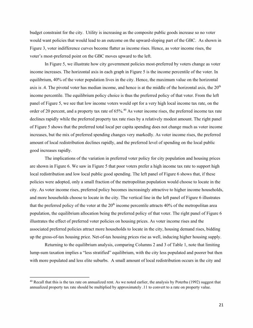
In Figure 5, we illustrate how city government policies most-preferred by voters change as voter

income increases. The horizontal axis in each graph in Figure 5 is the income percentile of the voter. In

equilibrium, 40% of the voter population lives in the city. Hence, the maximum value on the horizontal

axis is .4. The pivotal voter has median income, and hence is at the middle of the horizontal axis, the 20th

income percentile. The equilibrium policy choice is thus the preferred policy of that voter. From the left

panel of Figure 5, we see that low income voters would opt for a very high local income tax rate, on the

order of 20 percent, and a property tax rate of 65%.40 As voter income rises, the preferred income tax rate

declines rapidly while the preferred property tax rate rises by a relatively modest amount. The right panel

of Figure 5 shows that the preferred total local per capita spending does not change much as voter income

increases, but the mix of preferred spending changes very markedly. As voter income rises, the preferred

amount of local redistribution declines rapidly, and the preferred level of spending on the local public

good increases rapidly.

The implications of the variation in preferred voter policy for city population and housing prices

are shown in Figure 6. We saw in Figure 5 that poor voters prefer a high income tax rate to support high

local redistribution and low local public good spending. The left panel of Figure 6 shows that, if these

policies were adopted, only a small fraction of the metropolitan population would choose to locate in the

city. As voter income rises, preferred policy becomes increasingly attractive to higher income households,

and more households choose to locate in the city. The vertical line in the left panel of Figure 6 illustrates

that the preferred policy of the voter at the 20th income percentile attracts 40% of the metropolitan area

population, the equilibrium allocation being the preferred policy of that voter. The right panel of Figure 6

illustrates the effect of preferred voter policies on housing prices. As voter income rises and the

associated preferred policies attract more households to locate in the city, housing demand rises, bidding

up the gross-of-tax housing price. Net-of-tax housing prices rise as well, inducing higher housing supply.

Returning to the equilibrium analysis, comparing Columns 2 and 3 of Table 1, note that limiting

lump-sum taxation implies a “less stratified” equilibrium, with the city less populated and poorer but then

with more populated and less elite suburbs. A small amount of local redistribution occurs in the city and

                                                            40 Recall that this is the tax rate on annualized rent. As we noted earlier, the analysis by Poterba (1992) suggest that annualized property tax rate should be multiplied by approximately .11 to convert to a rate on property value.

 

22  

a very small amount in the poorer suburb, with a low income tax of 2.14% in the city.41 The pivotal voter

in the city is quite poor and has income slightly above the mean, choosing a tax package that deters richer

households to keep down the rental price of housing. The federal income tax drops by about 3%, and less

redistribution takes place overall. Property taxes rise everywhere substantially to finance the local public

good, not surprisingly given the loss of potential tax revenues from the lump-sum tax and the reluctance

to tax income. Some of the proceeds of the property tax are used to finance the small redistribution in the

city and the smaller yet redistribution in the poorer suburb. It bears emphasis that, when lump-sum taxes

are limited, we find the property tax rather than the income tax to be the local tax of choice. Comparing

Columns 2 and 3, we see that limiting lump sum taxation results in a decline in the levels of the local

public good in all communities, but the declines in the local values are somewhat misleading as the

sorting changes imply the economy per capita average level of local public good consumption declines by

only $241 (e.g., the rich suburb has many more households consuming a relatively large amount).

Motivated by the passage of property tax limits in some jurisdictions in the U.S., we also consider

the equilibrium with the same limit on local lump-sum taxes and with property taxes restricted to be no

higher than 35%, which, recall implies a much lower limit of about 3.2% on property value using the

Poterba conversion. This restriction on property taxes is in the range of observed property tax rates in the

U.S., which vary between about 0.2% and 4.5% of home value.42 Also, 48 states do limit property taxes,

the exceptions being Connecticut, Hawaii, New Hampshire, and Vermont. Rate limits impose maximum

rates on jurisdictions (e.g., counties, municipalities, and school districts) and apply to property market

value.43 Maximum authorized property tax rates range from 0.5 percent (Kentucky) to 5% (Michigan) of

property value.44 Hence, this 3.2% limit we impose is also within the range of actual property tax limits.

Equilibrium values with this property tax limit are reported in Column 4 of Table 1. Stratification is very

                                                            41 Although most local jurisdictions do not impose a local income tax, they are imposed by 4,943 jurisdictions in 17 states, or approximately 13% of all local jurisdiction. As mentioned above, the local income tax rates that arise in our model are within the range of empirically observed rates, which range from very 0.1% to almost 4.0%. In addition, in general local income taxes are levied by the central cities of metropolitan areas and not the suburbs. For instance, of these 17 states that have local income taxes, eight of them each have a total of 3 or less jurisdictions with income taxes, and almost all of these particular jurisdictions are central cities in metropolitan areas. If suburbs in a metropolitan area do impose income taxes, the rates for the most part are less than the central city’s. For instance, almost 60% of the local jurisdictions that impose income taxes are in Pennsylvania and most of these 2,621 jurisdictions impose income taxes not exceeding 2%. The six cities that impose higher rates (Philadelphia 3.98%, Scranton 3.4%, Pittsburgh 3%, Wilkes-Barre 2.85%, and Reading 2.7%) are all central cities in metropolitan areas. In Kentucky, where 218 local jurisdictions impose income taxes, the highest rates are in the central cities of the two major metropolitan areas, which are Louisville 2.2% and Lexington 2.25% (Henchman and Sapia, 2011). 42Siniavskaia, 2016. 43Tax Policy Center Foundation, Urban Institute and Brookings Institution, Tax Policy Center Briefing Book, Sate (and Local) Taxes, http://www.taxpolicycenter.org/briefing-book/what-are-tax-and-expenditure-limits 44Advisory Commission on Intergovernmental Relations, 1995(a). Tax and Expenditure Limits on local Governments. Washington, D.C. 

23  

similar to the previous case. Property taxes are at the bound in each local jurisdiction. A moderate local

income tax of 3.62% arises in the city, with per capita revenues of $882 split between financing a small

local redistribution ($500) and the rest put toward financing the local public good. No local redistribution

takes place in either suburb, though a small income tax arises in the poorer suburb to help finance the

local public good there. Both suburbs have lump-sum taxation, with the rich suburb at the bound. Local

public good levels decline given the restrictions on tax instruments and the reluctance to tax income,

especially in the suburbs.45 Property taxation still dominates local finance. The federal tax increases a

little as the pivotal federal voter (i.e., median income household) anticipates less (negative) redistribution

in his community, the poorer suburb.

Ignoring the fifth column for the moment, which is mainly of interest for its normative

implications, consider the effects of reducing mobility. Table 2 presents equilibrium values as in Table 1

for the several policy regimes but assuming one-half of each income type are mobile ( (y) .5 ) , i.e.,

can costlessly relocate jurisdictions after their initial choice and local voting. Table A1 in the appendix

presents the same with only 1% of each income type mobile (i.e., with (y) .01 ). The main point is

that the same fundamentals carry over, i.e., little or no local redistribution and little or no local income

taxation. Focusing on the case of 50% mobility, considering the main cases of interest in Columns 2,3,

and 4, observe that in only the two cases with lump-sum taxation restricted does any local redistribution

arise and only in the city. For example, with just a restriction on local lump-sum taxation (Column 3),

city residents obtain a locally financed lump-sum redistribution of $695, financed by a small local income

tax just below 1% and with some of the proceeds from the local property tax. Imposing also the property

tax ceiling of 35% (Column 4), the city lump-sum redistribution drops to just $263. The income tax rises

in the city to 2.82%, but about half of the proceeds from it are used to help finance the local public good

given the property tax limit. The only other case of any local income tax is in the latter case in the poorer

suburb, but with all the proceeds from the 1.65% local income tax supplementing provision of the local

public good. The lack of local redistribution carries over to the case of virtually no mobility (see Table

A1): With only 1% mobile, in none of the cases we examine is there any local redistribution. With both

the local lump-sum tax and property tax restrictions, small local income taxes arise, but to help finance

the local public goods. We can infer that the potential for relocation is not the explanation for limited or

no local redistribution. As we have discussed, it is the weak incentive to redistribute locally resulting

from income sorting that explains this finding.

                                                            45 The economy per capita local public good consumption equals $4,244 in this case, as compared to $6,273 in the previous case with just the local lump-sum tax constrained. These per capita consumption levels for all cases are available from the authors.

24  

Restricting mobility does have some other equilibrium effects. Sorting is a bit different, but not

much. Interestingly, the federal income tax rate rises some, e.g., from 11.7% to 13.5% as mobility drops

form 100% to 50% for the case with just the restriction on the local lump-sum tax (Columns 3 in Tables 1

and 2). The higher federal income tax discourages local income taxation because it exacerbates the

income tax distortion. Actually, the net effects yield higher income redistribution as mobility is reduced.

4.2.2. Normative Analysis. We return to the case of 100% mobility with a normative focus. Using the

unitary state as the baseline, we measure welfare as the sum of average EV plus the change in housing

rents, the latter since we have absentee housing owners. Refer to the lower entries in Table 1. Note that

in all cases either the welfare effect on households and housing owners is the same sign, or the effect on

households dominates. In any case, we report both effects (i.e., we report EV and EV plus housing rents).

We also report the income range that is worse off with the regime change, and, in Figure 4, graph EV as a

function of income. As seen in Column 2 of Table 1, the federal system with no tax restrictions leads to

an average welfare gain, but a large majority of poorer households (82.3%) are worse off. Average

welfare rises because of the efficiencies from Tiebout-type sorting, also with relatively efficient taxation,

in particular heavy reliance on local lump-sum taxes. Local lump sum taxes are efficient both because

they are non-distortionary and because they induce relatively efficient household sorting, the latter

because they efficiently price community access in as much as they equal the cost of the local public good

(see, e.g., Calabrese, Epple, and Romano, 2012). Direct redistribution is a little higher in the federal

equilibrium than in the unitary state, but all those in the city in the former regime (71.6%) consume

substantially less of the local public good, implying a net welfare loss.46 In short, there is an equity-

efficiency trade off in this comparison.

Examining Columns 3 and 4 of Table 1, one sees that in the cases of the federation with the lump-

sum tax restrictions, welfare is lower than in the unitary state and either everyone or almost everyone is

worse off! This finding generalizes the main result in Calabrese, Epple, and Romano (2012). In the

latter, we show that Tiebout equilibria that restrict local taxes to property taxes are inefficient. We show

that this is explained by inefficient sorting that results, which increases the costs of free riding in

consumption of local public goods, to the determinant of almost everyone. This is shown by

demonstrating that directly restricting access of poorer households to richer jurisdictions, with otherwise

equilibrium choices (e.g., majority choice of local property taxes), produces welfare gains. The welfare

losses we find here generalize this finding in two ways. The present model also has a central government,

not presents in our 2012 paper. Here, choice of local property taxation is endogenous, i.e., in these cases

local income taxation is an option, while we assumed only property taxation in the 2012 paper.

                                                            46 The housing price in the city in the federal equilibrium is lower than in the unitary state, so this effect pulls for gains to the poorer households.

25  

Consider last the equilibrium in Column 5 of Table 1. This is a Tiebout equilibrium, with no

central government, and with no restrictions on the local tax instruments.47 We study such equilibria in

CER (2015). Observe that this is the most efficient allocation, which means that having a central

government with power to redistribute is inefficient. It is natural to compare this equilibrium to that in

Column 2, with the latter adding the federal government to the Tiebout equilibrium. One can see that the

equilibria are quite similar (e.g., sorting is close), the key difference just being the federal income tax and

associated redistribution in the federal case. Creating scope for central government to redistribute lowers

efficiency and also hurts the rich and upper middle class. However, poorer households, specifically those

with income below $52,150 are better off in the case with the federal government. Introducing the federal

government entails, again, an equity-efficiency trade off.

Another normative perspective, presented in Figure 5, shows the distribution of “generalized

consumption” in the policy regimes, which we define to equal expenditure on private goods plus

consumption of the local public good. We omit the federal regime with both of the tax limits just to

reduce clutter. One can see that, relative to the unitary state (this distribution included in the graph), the

two federal regimes and the pure Tiebout regime (no central government) have a greater proportion of

households with very low generalized consumption, with the Tiebout regime the least equitable in this

regard. The federal regime with restricted lump-sum taxation has the most households with generalized

consumption above $83,387.48 One might expect the federal regime with no tax restrictions and the pure

Tiebout regime would have the largest group with very high generalized consumption, but the substantial

lump-sum tax in the rich suburb in these regimes curtails very high consumption by other than the very

rich. One can also see that the pure Tiebout regime has the widest generalized consumption distribution

followed by the federal regime with limited lump-sum taxation.

All the normative comparisons are qualitatively analogous in the cases of restricted mobility, as

can been seen in Tables 2 and A1.

                                                            47 To compare our findings on redistribution to Epple and Romer (1991), another model variation we have considered is that with no central government and with the restriction on local lump-sum taxation. Epple and Romer (1991) find significant local income redistribution in a one-tiered multi-community Tiebout model that assumes local property taxation. Our model with no central government, limited lump-sum taxation, and 100% mobility is most similar, though it allows local income taxation in addition to property taxation. Nevertheless, we obtain substantially less local redistribution than Epple and Romer (1991). The explanation is that our model has a local public good whereas Epple and Romer (1991) does not. In our equilibrium, provision of the local public good increases the distortion if property taxes are to be increased to provide local redistribution, and hardly any results. Nor are income taxes used due to their distortion. We confirm this logic by showing that local redistribution increases as the weight on the local public good in the utility function declines. This analysis is available on request. 48 The $83,387 is the minimum generalized consumption among residents in the richest suburb in this regime, at the rightward jump in the distribution (see Figure 5). In the cases with multiple communities (i.e., other than the unitary state), jumps in the distribution occur at community boundary incomes, but, in the cases with significant lump-sum taxation, they are not very apparent.

26  

4.2.3. Housing Owners. We have so far assumed households rent housing. Housing owners will have

weaker incentives to tax property, so it is of interest to examine whether home ownership alters our main

findings, especially the reluctance to employ local income taxes. To investigate this, we adapt the home-

ownership specification in CER (2015) to the present model. We assume all households are owners, or,

otherwise, existence issues arise. Refer to Figure 1. Stage 1 is the same. Stage 2 is modified to have

households sign a contract with a competitive housing supplier in the community they initially select to

build them a house in Stage 5 of quality/quantity h, at agreed upon price per unit of h. The contract may

be renegotiated in Stage 5 when housing is actually built and consumed. The price in the contract must

equal the ultimate equilibrium housing price since all agents have rational expectations, but it is

convenient to have different notation for the equilibrium contract price, jh1p . Stages 3 and 4 are the same

as with renters. While no capital gains or losses arise on the equilibrium path, relocation by mobile

households and consumption adjustments for out-of-equilibrium policies could change the supplier price

of housing. Specifically, housing value would change by j jh h1(p p )h, out of equilibrium. In Stage 5,

households optimally “buy out” of their housing contract and adjust consumption to the level of h equal to

demand at price j jh(1 t )p and with income including capital gain/loss equal to j j

h h1(p p )h. Housing

suppliers are just as well off under the buy-out, and owners are better off.49 If j jh h1p p , owners

experience a capital gain. The housing supplier is just as well off paying the buyer j jh h1(p p )h to not

build since the supplier can instead supply h at equilibrium price jhp . If j j

h h1p p , then the buyer must

compensate the supplier j jh1 h(p p )h to not build as agreed upon. Buyers are better off since they can

adjust their housing consumption reflecting the change in housing price. Note that these prospective

capital gains/losses imply the full incidence of property taxes falls on buyers. For tractability, we maintain

the utility taking assumption regarding how a voter assesses utility in other jurisdictions of movers.

The only difference in the primitive equations (i.e., (2)-(7)) is that f j f jy[1 (1 ω(m m ))(m m )] is replaced for non-movers everywhere by

f j f j j j jh h1 dy[1 (1 ω(m m )(m m )] (p p )h (y,p ), where we assume households contract for their

equilibrium preferred level of housing initially.50 While no capital gain/loss arises in equilibrium, the

potential for a gain or loss will have a marked effect on equilibrium policies. In particular, in

                                                            49 One might alternatively assume suppliers and buyers share in capital gains/losses, by specifying the capital gain/loss to buyers equal to j j

h h1θ (p p )h, with θ (0,1); and with the remainder accruing to the supplier. 50 This is an optimal choice since no capital gains or losses actually materialize in equilibrium. As above, we continue to write hd(y,p) for housing demand, but the relevant y is after taxes and any capital gains.

27  

contemplating the effects of voting on the property tax, the capital gains/losses that arise out-of-

equilibrium make owners relatively averse to property taxation. As shown in the on-line appendix,

indirect utility is modified to be:

(12)

j j j jo o o o

j j f j f j j j j jo h h1

j j j j j j jo h h1

j

V(Γ ,Ω , y) y Γ Ω ;

Γ v(g ) [1 (1 ω(m m ))(m m )] [1 (p p )G(p )] w(p );Ω v(g ) r [1 (p p )G(p )] w(p );

where G (p ) 0.

The analysis and above propositions for the case of renters’ carries over to the owners’ case with jo and

jo everywhere replacing respectively j and j.

Turning to the computational analysis, we use the same calibration for a cleaner comparison to

the renters’ case, and we focus on the case with all households mobile. For tractability in the

computational analysis, we assume households consider only their own capital gains/losses and that their

housing contracts are voided if they relocate.51 Table 3 summarizes positive and normative properties of

equilibrium in the same policy regimes as in Tables 2 and 3, but omitting the case with no central

government (available from the authors). Equilibrium exists in all the cases presented here, so we again

find equilibrium in interesting cases. The Unitary State Case is presented in Column 1 and the federal

case with no tax restrictions in Column 2. Comparing these respectively to Columns 1 and 2 of Table 1

for renters, a salient effect is lower property tax rates, with the exception of the richest suburb in the

federal cases. The property tax rate is, however, quite low in the latter cases. No local redistribution

arises in the federal case with owners, and local property taxes are 0 in each jurisdiction. The federal

income tax rates change little. Considering restrictions on local taxes, existence of equilibrium fails if the

local lump-sum tax level is severely restricted. We then examine the case with local lump-sum taxes

restricted to be no higher than 20% of expenditure on the local public good, where equilibrium exists.

Equilibrium values for owners with just this restriction in the federal system are presented in Column 3 of

Table 3. For comparison, the equilibrium with renters and the same restriction is presented in Column 5.

No local redistribution results with owners. A small property tax (1.88%) arises in the richer suburb,

which helps to finance the local public good there. Property tax rates are lower in the city and in the

richer suburb in the owners’ case, though somewhat higher in the poorer suburb with owners. The federal

income tax is about the same. Imposing the property tax rate restriction (Column 4), lowers the property

                                                            51 The first part of this simplification means that voters do not anticipate income effects of others’ capital gains or losses off the equilibrium path. The second simplification means that voters do not realize capital gains or losses if they relocate, again off the equilibrium path, this consistent with the utility taking assumption (though not to suggest this is realistic).

28  

tax to the bound in the city and poorer suburb, induces small local income taxes, and leads to less of the

local public good provided in these two jurisdictions.

The normative comparisons and interpretations are the same as with renters. Restricting mobility

has similar effects to doing so with renters, and, in particular, does not lead to local redistribution.52 In

short, all the main qualitative results regarding renters carry over to owners.

5. Concluding Remarks

We have provided a model with two tiers of government, multiple local jurisdictions, households that

differ by income with at least some able to move among local jurisdictions, and with majority choice of a

redistributive linear income tax at both tiers. In addition, property taxation and lump-sum taxes in local

jurisdictions are majority selected, in some cases with limits, the proceeds used to finance a local public

good and/or local redistribution. Assuming a household utility function that is homogenous of degree 1 in

the numeraire and housing consumption and multiplicative in the local public good, we show theoretically

that: (i) an indirect utility function that is linear in income over two composite public goods arises, their

values depending on all taxes, the level of the housing price, and expenditure on the local public good; (ii)

majority choice of local tax instruments exists given the federal income tax and federal redistribution; and

(iii) income stratification across jurisdictions arises assuming equilibrium exists; and (iv) we provide an

algorithm for determining and confirming majority choice of the federal income tax. We then specify a

quantitative model that we use to confirm equilibrium and explore its properties. We show equilibrium

does exist in a series of examples that vary with respect to the degree of mobility of households, whether

there are tax limits, and whether households rent or own housing. We find the equilibrium has little or no

local redistribution and very limited use of local income taxation. We show that the explanation for the

lack of local redistribution is weak local incentives to do so, this driven by income sorting. We show a

preference for local property taxation over local income taxation, whether or not households rent of own

housing. Normative findings are these: (v) assuming local lump-sum taxes are permitted, equilibrium

with no central government is more efficient but less equitable than the federal system equilibrium; (vi)

the latter federal system is, however, more efficient but less equitable than having just a central

government; and (vii) a federal system with highly constrained local lump-sum taxes is inefficient and

inequitable relative to having just a central government.

The model has limitations, and we conclude with discussion of some of these and challenges that

arise in addressing them. In our model, household heterogeneity is just with respect to income and

whether or not a household can costlessly relocate. Introducing preference heterogeneity over local

                                                            52 This analysis is available from the authors, as well as the analogues to Figures 4 and 5.

29  

public goods or for locations can be expected to induce some degree of income mixing. This might

increase incentives for local redistribution. The challenge in extending our model to have such difference

in preferences regards existence of equilibrium. We have not considered taxation of the numeraire, i.e.,

sales taxes, at either the federal of local level. As discussed in CER (2015), local majority choice of sales

taxes does not disrupt local majority choice equilibrium, but it would not arise if households can travel

costlessly among local jurisdictions to consume the numeraire. We have not considered a model with

frictions in this. Federal sales taxation or any other federal taxation is of interest to examine. One might

also consider provision of a national public good and/or federal subsidies to local public goods. We think

that Proposition 3 can be extended to investigate a greater federal role, though existence is not assured

and the problem is challenging computationally. We believe that progress can be made on these various

extensions, but are topics for future research.

30  

References

Advisory Commission on Intergovernmental Relations, Tax and Expenditure Limits on local Governments. Washington, D.C. (1995). Advisory Commission on Intergovernmental Relations, Local Revenue Diversification: Local Income Taxes. Staff report, Washington, D.C (1988).

Baicker, Katherine, Jeffrey Clemens, and Monica Singhal, “The Rise of the States: U.S. Fiscal Decentralization in the Postwar Period,” Journal of Public Economics, 96 (2012), 1079-1091.

Benabou, Roland, “Equity and Efficiency in Human Capital Investment: The Local Connection,” Review of Economic Studies, 63 (1996), 237-264.

_______, “Workings of a City: Location, Education, and Production,” Quarterly Journal of Economics, 108 (1993), 619-652.

Boadway, Robin, 1982. “The method of taxation and the provision of local public goods: comment. Am. Econ. Rev. 72(4), 846-851.

Boadway, Robin, Maurice Marchand, and Marianne Vigneaulty, “The Consequences of Overlapping Tax Bases for Redistribution and Public Spending in a Federation,” Journal of Public Economics, 68(1998), 453-478.

Brueckner, Jan, 1983. Property value maximization and public sector efficiency. J. Urban Econ. 14(1), 1-15. __________, 2004. Fiscal decentralization with distortionary taxation: Tiebout vs. tax competition. International Tax and Public Finance 11(2), 133-153. Bucovetsky, Sam, “Choosing Tax Rates and Public Expenditure Levels Using Majority Rule,” Journal of Public Economics, 46 (1991), 113-131.

Calabrese, Stephen, Glenn Cassidy, and Dennis Epple, “Local Government Fiscal Structure and Metropolitan Consolidation,” Brookings-Wharton Papers on Urban Affairs, 2002, 1-43.

Calabrese, Steve, Dennis Epple, and Richard Romano, “On the Political Economy of Zoning,” Journal of Public Economics, 91 (February 2007), 25-49. ____________________________, “Inefficiencies from Metropolitan Political and Fiscal Decentralization: Failures of Tiebout Competition,” Review of Economic Studies, 79 (July 2012), 1081-1111. ____________________________, “Majority Choice of Tax Systems in Single- and Multi-Jurisdictional Economies,” Journal of Public Economics, 131 (November 2015), 58-70.

deBartolome, Charles, “Equilibrium and Inefficiency in a Community with Peer Group Effects,” Journal of Political Economy, 98 (1990), 110-133.

deBartolome, Charles and Stephen L. Ross, “The Race to the Suburb: The Location of the Poor in a Metropolitan,” 2002, University of Connecticut Working Paper #2002-02.

Department of Commerce, Bureau of Census, Historical Statistics on Governmental Finances and Employment, an annual report, Government Finances (1968).

31  

Ellickson, Robert C., “Jurisdictional Fragmentation and Residential Choice,” American Economic Review, 61, 2 (1971), 334-339.

Epple, Dennis, Filimon, Radu, and Romer, Thomas, 1984. Equilibrium among local jurisdictions: toward an integrated treatment of voting and residential choice. J. Public Econ. 24(3), 281-399.

Epple, Dennis, Brett Gordon, and Holger Sieg, “A New Approach for Estimating the Housing Production Function,” American Economic Review, 100, 1(June 2010), 905-924.

Epple, Dennis and Glenn Platt, “Equilibrium and Local Redistribution in an Urban Economy when Households Differ in both Preferences and Incomes,” Journal of Urban Economics, 43,1 (1998), 23-51.

Epple, Dennis and Richard Romano, “Public School Choice and Finance Policies, Neighborhood Formation, and the Distribution of Educational Benefits,” Chapter 7 in The Economics of School Choice, Caroline Hoxby, ed., National Bureau of Economic Research, University of Chicago Press, 2003, 227-286.

Epple, Dennis, Richard Romano, and Holger Sieg, “The Intergenerational Conflict over the Provision of Public Education,” Journal of Public Economics, 96 (April 2012), 255-268.

Epple, Dennis and Thomas Romer, “Mobility and Redistribution,” Journal of Political Economy, 99 (August 1991), 828-858.

Epple, Dennis and Allan Zelenitz, “The Implications of Competition among Jurisdictions: Does Tiebout Need Politics?” Journal of Political Economy, 89, 6 (1981), 1197-1217.

Feldstein, Martin, “Tax Avoidance and the Deadweight Loss of the Income Tax,” The Review of Economics and Statistics, 81, 4 (November 1999), 674-680.

Feldstein, Martin and Marian Wrobel, “Can State Taxes Redistribute Income,” Journal of Public Economics, 68 (1998), 369-396.

Fernandez, Raquel and Richard Rogerson, “Income Distribution, Communities, and the Quality of Public Education,” Quarterly Journal of Economics, 111, 1(February 1996), 135-164.

________________________ , “Public Education and Income Distribution: A Quantitative Analysis of Education Finance Reform,” American Economic Review, 88 (1998), 813-833.

Goodspeed, Timothy J., “Local Income Taxation: An Externality, Pigouvian Solution, and Public Policies,” Regional Science and Urban Economics, 25 (1995), 279-296.

Gordon, Roger H., “An Optimal Taxation Approach to Fiscal Federalism,” Quarterly Journal of Economics, 98 (1983), 567-586.

Gordon, Roger H. and Julie Cullen, “Income Redistribution in a Federal System of Governments,” Journal of Public Economics, 96 (2012), 1100-1109.

Grandmont, Jean-Michel, “Intermediate Preferences and the Majority Rule,” Econometrica, 46, 2 (March 1978), 317-330.

Hamilton, Bruce, “Zoning and Property Taxation in a System of Local Governments,” Urban Studies, 1-2 (June 1975), 205-211.

32  

Hansen, Nico and Anke Kessler, “The Political Geography of Tax H(e)avens and Tax Hells,” American Economic Review, 91 (September 2001), 1103-1115.

Harmon, Oskar R., “The Income Elasticity of Demand for Single-Family Owner-Occupied Housing: An Empirical Reconciliation,” Journal of Urban Economics, 38 (1988), 75-85.

Henchman, Joseph and Jason Sapia, “Local Income Taxes: City- and County-Level Income and Wage Taxes Continue to Wane,” Fiscal Fact, Tax Foundation, August 31, 2011, https://taxfoundation.org/local-income-taxes-city-and-county-level-income-and-wage-taxes-continue-wane/

Henderson, J. Vernon, “Community Choice of Revenue Instruments,” Regional Science and Urban Economics, 24, 2 (1994), 159-183.

Inman, Robert, “The Local Decision to Tax: Evidence from Large U.S. Cities,” Regional Science and Urban Economics, 19, 3(1989), 455-491.

Inman, Robert and Daniel Rubinfeld, “Designing Tax Policies in Federalist Economies: An Overview,” Journal of Public Economics, 60 (1996), 307-334.

Johnson, William, “Income Redistribution in a Federal system,” American Economic Review, 78 (June 1988), 57-573.

Kessler, Anke and Chritoph Lulfesmann, “Tiebout and Redistribution in a Model of Residential and Political Choice,” Journal of Public Economics, 89 (2005), 501-528.

Krelove, Russell, “The Persistence and Inefficiency of Property Tax Finance of Local Public Expenditures,” Journal of Public Economics, 51 (July 1993), 415-435.

Lockwood, Ben, “Fiscal Decentralization: A Political Economy Perspective,” Handbook of Fiscal Federalism, E. Ahmad and G. Brosio, eds., Edward Elgar, 2006. Meltzer, Alan and Scott Richard, “A Rational Theory of the Size of Government,” Journal of Political Economy, 89 (1981), 914-927.

Musgrave, Richard A., “Economics of Fiscal Federalism,” Nebraska Journal of Economics and Business, 10 (1971), 3-13.

Nechyba, Thomas, “Local Property and State Income Taxes: The Role of Interjurisdictional Competition and Collusion,” Journal of Political Economy, 105, 2 (1997), 351-384.

__________, “School Finance Induced Migration Patterns: The Impact of Private School Vouchers,” Journal of Public Economic Theory, 1,1 (1999), 5-50.

__________, “Mobility, Targeting, and Private School Vouchers,” American Economic Review, 90, 1 (2000), 130-46.

Oates, Wallace E, Fiscal Federalism, 1972a, New York: Harcourt Brace Jovanovich. ___________, “An Economist’s Perspective on Fiscal Federalism,” in Oates, W.E. (Ed), The Political Economy of Fiscal Federalism, Lexington, MA, D.C. Heath, 1972b, 3-20. ___________, “An Essay on Fiscal Federalism,” Journal of Economic Literature, 37 (September 1999), 1120-1149.

33  

Plott, Charles, “A Notion of Equilibrium and its Possibility under Majority Rule,” American Economic Review, 57, 4 (September 1967), 787-806.

Poterba, James, “Taxation and Housing: Old Questions, New Answers,” American Economic Review, 82, 2 (1992), 237-242.

Rohrs, Sigrid and David Stadelmann, “Homeownership, Mobility, and Local Income Redistribution,” Journal of Public Economic Theory, 16 (August 2014), 569-605.

Siniavskaia, Natalia, “Property Tax Rates in and Within Counties,” Economics and Housing Policy Group, National Association of Home Builders, Special Studies, April 1, 2016 www.nahb.org

Stigler, George, “The Tenable Range of Functions of Local Government,” Joint Economic Committee, Federal Expenditure Policy for Economic Growth and Stability. U.S. Government Printing Office, Washington, D.C., 1957, 213-219.

Tax Policy Center Foundation, Urban Institute and Brookings Institution, Tax Policy Center Briefing Book, Sate (and Local) Taxes, http://www.taxpolicycenter.org/briefing-book/what-are-tax-and-expenditure-limits

Tax Foundation, Local Income Tax Rates by Jurisdiction, 2011. Compilation from State revenue departments and other sources. www.TaxFoundation.org

Tiebout, Charles. M., “A Pure Theory of Local Expenditures,” Journal of Political Economy, 64 (1956), 416-424.

Westhoff, Frank, “Existence of Equilibrium in Economies with a Local Public Good,” Journal of Economic Theory, 14 (February 1977), 84-112.

Wildasin, David, “Locational Efficiency in a Federal System,” Regional Science and Urban Economics, 10 (1980), 453-471.

____________, “Income Redistribution in a Common Labor Market,” American Economic Review, 81 (September 1991), 757-774.

Wilson, J., “Property Taxation, Congestion, and Local Public Goods,” Journal of Public Economics, 64 (1997), 207-217.

Wooders, Myrna, “The Tiebout Hypothesis: Near-optimality in Local Public Good Economies,” Econometrica, 48 (1980), 1467-1485.

Zodrow, George, “The Incidence of Metropolitan Property Tax Base Sharing and Rate Equalization,” Journal of Urban Economics, 15, 2(1984), 210-229.

34  

Figure 1 Stage 1 Stage 2 Stage 3 Stage 4 Stage 5

All Households Vote on Federal

Income Tax

Households Choose Initial

Local Jurisdiction

Households Vote Over Local Policy

Mobile Households Costlessly Relocate

Households Consume,

Government Budgets Balance,

Markets Clear

 

 

 

 

Ωj  

Figure 2: Equilibrium in Community j  

Γj  

Indifference Curve of 

Median Income Household 

in Community j  

Equilibrium 

GBCj   

.  

35  

 

 

 

 

 

 

 

 

 

 

36  

 

Figure 4  

 

 

 

 

 

 

 

 

 

 

 

Government Budget Constraint for the City

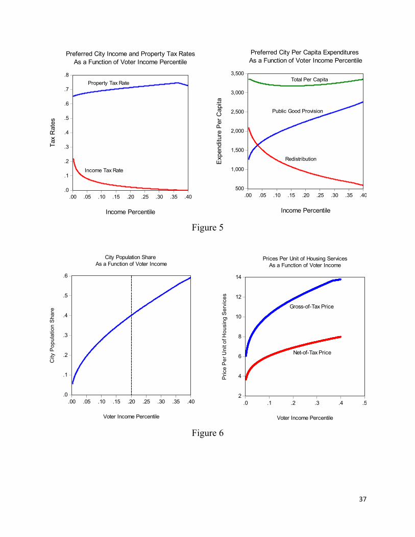
37  

 

Figure 5  

 

Figure 6  

   

.0

.1

.2

.3

.4

.5

.6

.7

.8

.00 .05 .10 .15 .20 .25 .30 .35 .40

Preferred City Income and Property Tax RatesAs a Function of Voter Income Percentile

Income Tax Rate

Property Tax Rate

Tax

Rat

es

Income Percentile

500

1,000

1,500

2,000

2,500

3,000

3,500

.00 .05 .10 .15 .20 .25 .30 .35 .40

Redistribution

Public Good Provision

Total Per Capita

Income PercentileE

xpen

ditu

re P

er C

apita

Preferred City Per Capita Expenditures As a Function of Voter Income Percentile

.0

.1

.2

.3

.4

.5

.6

.00 .05 .10 .15 .20 .25 .30 .35 .40

Voter Income Percentile

City

Po

pu

latio

n S

ha

re

City Population Share As a Function of Voter Income

2

4

6

8

10

12

14

.0 .1 .2 .3 .4 .5

Voter Income Percentile

Pri

ce P

er

Un

it o

f Ho

usi

ng

Se

rvic

es

Prices Per Unit of Housing ServicesAs a Function of Voter Income

Net-of-Tax Price

Gross-of-Tax Price

34  

35  

36  

 

Table 1: Renters' Model w. 100% Mobility* 

     Unitary State 

 

 

Fed. System Fed. System Lump‐Sum 

Fed. System Local Lump‐Sum and Property  No Central 

   No Tax Limits  Tax Limits**  Tax Limits***  Government 

Positive Properties   

n1 =   100%  71.6%  40.0%****  41.6%****  70.8% 

  n2 =   n/a  23.0%  30.0%  28.6%  23.7% 

  n3 =   n/a  5.4%  30.0%  29.8%  5.6% 

  t1 =  84.7%  54.0%  71.4%  35.0%  53.1% 

  t2 =  n/a  15.8%  61.3%  35.0%  17.1% 

  t3 =  n/a  4.9%  79.5%  35.0%  6.4% 

  m1 =  n/a  0.0%  2.1%  3.6%  0.0% 

  m2 =  n/a  0.0%  0.0%  1.9%  0.0% 

  m3 =  n/a  0.0%  0.0%  0.0%  0.0% 

  r1 =  n/a  ($349)  $939  $500  ($378) 

  r2 =  n/a  ($7,779)  $96  ($69)  ($8,168) 

  r3 =  n/a  ($22,845)  ($630)  ($369)  ($25,506) 

  g1 =  $4,799  $3,500  $2,248  $2,031  $3,276 

  g2 =  n/a  $10,549  $4,500  $4,187  $11,424 

  g3 =  n/a  $24,832  $12,609  $7,383  $28,553 

  mf =  11.4%  14.8%  11.7%  12.3%  n/a 

  rf =  $9,415  $9,535  $7,641  $7,940  n/a 

Norm. Props.*****    EV =  n/a  $553  ($1,250)  ($1,581)  $3,967 

EV+ΔHouse Rents=   n/a  $1,167  ($1,182)  ($965)  $4,723 

Interval Worse Off  n/a  <  $102,800  < $228,000  All Incomes  < $59,700 

% Worse Off =  n/a  82.4%  97.4%  100.0%  59.5% 

 

*Utility is g.10h.22b.78.  Economy income lognormal with mean $67,392 and median $49,267.   Tax distortion parameter ω = .247.  Community housing supply elasticities equal 3.  Community areas are L1 = .675, L2 = .206, and L3 = .120.  Median community income below mean except where community proportion bolded. 

 

**rj ≥ ‐.05gj, j = 1,2,3. ***rj ≥ ‐.05gj, tj ≤ 35%, j = 1,2,3. ****Median community income exceeds mean. *****Positive (negative) EV and EV + ΔHouse Rents indicate average welfare gains (losses). 

 

   

 

37  

Table 2: Renters' Model w. 50% Mobility* 

     Unitary State 

 

 

Fed. System Fed. System Lump‐Sum 

Fed. System Local Lump‐Sum and Property  No Central 

   No Tax Limits  Tax Limits**  Tax Limits***  Government 

Positive Properties   

n1 =   100%  67.7%  43.6%****  44.9%****  66.5% 

  n2 =   n/a  24.1%  28.1%  27.5%  24.8% 

  n3 =   n/a  8.3%  28.3%  27.6%  8.6% 

  t1 =  84.7%  50.7%  71.4%  35.0%  50.2% 

  t2 =  n/a  22.9%  59.6%  35.0%  24.0% 

  t3 =  n/a  16.1%  69.6%  35.0%  17.7% 

  m1 =  n/a  0.0%  1.0%  2.8%  0.0% 

  m2 =  n/a  0.0%  0.0%  1.7%  0.0% 

  m3 =  n/a  0.0%  0.0%  0.0%  0.0% 

  r1 =  n/a  ($528)  $695  $263  ($515) 

  r2 =  n/a  ($5638)  $(34)  ($195)  ($5,830) 

  r3 =  n/a  ($14,804)  ($590)  ($338)  ($16,225) 

  g1 =  $4,799  $3,416  $2,388  $2,184  $3,138 

  g2 =  n/a  $9,113  $4,736  $4,375  $9,728 

  g3 =  n/a  $20,213  $11,804  $7,554  $22,989 

  mf =  11.4%  14.9%  13.5%  13.7%  n/a 

  rf =  $9,415  $9,590  $8,733  $8,574  n/a 

Norm. Props.*****    EV =  n/a  $459  ($1,295)  ($1,520)  $3,828 

EV+ΔHouse Rents=   n/a  $1,031  ($1,168)  ($914)  $4,531 

Interval Worse Off  n/a  <  $98,900  All Incomes  All Incomes  < $58,500 

% Worse Off =  n/a  81.1%  100%  100.0%  58.5% 

 

*Utility is g.10h.22b.78.  Economy income lognormal with mean $67,392 and median $49,267.   Tax distortion parameter ω = .247.  Community housing supply elasticities equal 3.  Community areas are L1 = .675, L2 = .206, and L3 = .120.  Median community income below mean except where community proportion bolded. 

 

**rj ≥ ‐.05gj, j = 1,2,3. ***rj ≥ ‐.05gj, tj ≤ 35%, j = 1,2,3. ****Median community income exceeds mean. *****Positive (negative) EV and EV + ΔHouse Rents indicate average welfare gains (losses). 

   

38  

Table 3: Owners' Model w. 100% Mobility* 

     Unitary State 

 

 

Fed. System Fed. System Lump‐Sum 

Fed. System Local Lump‐Sum and Property 

 Renters’ 

Fed. System Lump‐Sum Tax Limits** 

   No Tax Limits  Tax Limits**  Tax Limits***   

Positive Properties   

n1 =   100%  79.0%  59.8%  55.8%  51.5% 

  n2 =   n/a  15.4%  22.8%  24.9%  30.0% 

  n3 =   n/a  5.6%  17.4%  19.3%  18.6% 

  t1 =  53.1%  9.3%  43.3%  35.0%  73.7% 

  t2 =  n/a  2.1%  76.9%  35.0%  53.6% 

  t3 =  n/a  8.4%  20.9%  25.7%  85.9% 

  m1 =  n/a  0.0%  0.0%  0.1%  0.0% 

  m2 =  n/a  0.0%  0.0%  0.5%  0.0% 

  m3 =  n/a  0.0%  1.9%  1.2%  0.0% 

  r1 =  n/a  ($3,099)  ($594)  ($502)  $594 

  r2 =  n/a  ($9,400)  ($1,717)  ($1,049)  ($1,267) 

  r3 =  n/a  ($14,871)  ($2,132)  ($1,998)  ($3,596) 

  g1 =  $4,642  $3,878  $2,968  $2,512  $2,599 

  g2 =  n/a  $9,854  $8,586  $5,243  $6,336 

  g3 =  n/a  $18,366  $10,659  $9,990  $17,981 

  mf =  11.3%  13.9%  14.1%  16.2%  15.0% 

  rf =  $7,755  $8,960  $9,067  $10,340  $964 

Norm. Props.****    EV =  n/a  $568  ($738)  ($1,416)  ($959) 

EV+ΔHouse Rents=   n/a  $1,288  ($626)  ($1,143)  ($915)   Interval Worse 

Off  n/a  <  $95,600  > $27,100  > $37,400 > $19,350 <$302,900 

% Worse Off =  n/a  79.9%  72.4%  63.6%  87.0% 

 

*Utility is g.10h.22b.78.  Economy income lognormal with mean $67,392 and median $49,267.      Tax distortion parameter ω = .247.  Community housing supply elasticities equal 3.  Community    areas are L1 = .675, L2 = .206, and L3 = .120.  Median community income is less than mean in all cases. 

  **rj ≥ ‐.20gj, j = 1,2,3. 

  ***rj ≥ ‐.20gj, tj ≤ 35%, j = 1,2,3. ****Positive (negative) EV and EV + ΔHouse Rents indicate average welfare gains (losses).