Embed Size (px)
Citation preview
Optimal Call Center Staffing via Simulation
Conover, Arthur
Justice, Samuel
Lee, Aidan
Weiss-Christoff, Alexander
Advisor: Farnell, Elin
Department of Mathematics and Statistics, Kenyon College
April 22, 2016
Abstract
We discuss the methodology and results of a semester-long project in mathematical modeling, in
which we seek to create an optimal staffing plan for a call center for Nationwide Mutual Insurance
Company. The company provided data to use for this purpose along with the mandate that an optimal
staffing plan should staff a sufficient number of workers to answer 80% of calls within 30 seconds. We use
statistical models based on the data provided as input to Monte Carlo simulations in order to propose
an appropriate number of call service representatives needed for a given call type, day, and time interval.
Using these results, we explore potential approaches for devising staffing plans for the call center.
1 Introduction
In this paper, we discuss the results from a semester-long project for a course in mathematical modeling at
Kenyon College in Gambier, Ohio. This work was completed as part of the PIC Math Program (Preparation
for Industrial Careers in the Mathematical Sciences1). We seek to determine an optimal staffing plan for a
call center for Nationwide Mutual Insurance Company (hereafter Nationwide)2.
Like many businesses, Nationwide maintains a call center that allows customers to have their servicing
needs met via a phone conversation with a customer service representative. Nationwide expressed an interest
1Support for this Mathematical Association of America (MAA) and Society for Industrial and Applied Mathematics (SIAM)
program is provided by the National Science Foundation (NSF grant DMS-1345499).2Nationwide, a Fortune 100 company based in Columbus, Ohio, is one of the largest and strongest diversified insurance and
financial services organizations in the U.S. and is rated A+ by both A.M. Best and Standard & Poor’s. The company provides
a full range of insurance and financial services, including auto, commercial, homeowners, farm and life insurance; public and
private sector retirement plans, annuities and mutual funds; banking and mortgages; pet, motorcycle and boat insurance. For
more information, visit www.nationwide.com.
196
in finding ways to improve its short-term and long-term call-center staffing models. The short-term model
focuses on staffing the call center over the course of a given day, while the long-term model focuses on staffing
the call center over an entire year. Improvements in these areas would ideally help minimize both staffing
overages that lead to excess costs and staffing deficiencies that lower customer satisfaction. To address these
goals, Nationwide shared with us fictionalized details about the call center and a simulated sample of call
data. These materials were intended to provide a conceptually accurate portrayal of the staffing challenges
that Nationwide (and likely other companies) face without involving the use of sensitive or proprietary
information.
The call center is described as being open from 6 AM to 12 AM daily and is responsible for processing
a variety of calls related to the company’s business operations. In particular, the call center handles four
different types of calls, which we will refer to as Types A, B, C, and D. The content of each call type was not
provided by Nationwide due to confidentiality concerns. We assume that every call service representative at
Nationwide specializes in one of these four call types and exclusively answers the type of call in which he/she
specializes. Staffing needs are sensitive to several factors, including call type, time of day, day of week, and
time of year. Moreover, our analysis in this project is guided by Nationwide’s stated service-level agreement
to answer 80% of inbound calls within 30 seconds. For the rest of the paper, this customer service agreement
will be referred to as “successful operation.”
The simulated data set consisted of 105,396 observations based on the span of a year and a half from
July 1, 2013 to December 31, 2014. The data was aggregated at the half hour level, with each observation
in the data set designating both the number of calls and the average handle time of calls during a particular
30-minute interval for a given day of the year and call type. So, for example, one data point might tell us
the number and average handle time of Type B calls from 9:00 AM to 9:30 AM on June 21, 2014. The
definition of the number of calls is self-explanatory, but the definition of average handle time deserves special
attention. The average time required to handle a call includes both the actual phone call and the work that
the representative does afterward to process information related to the call.
We use the data provided to us by Nationwide to perform Monte Carlo simulations of daily call center
operations. We begin by creating sampling distributions for the number of calls, the handle time of each call,
and the time between each call based on the data. We then take random samples from these distributions
utilizing the statistical software R [5] and run simulations in C++. Employing a binary search algorithm in
our simulation enables us to quickly and efficiently find the minimum number of call service representatives
needed to ensure successful operations for all of the given time intervals and call types.
The paper proceeds as follows. We first discuss the details of our Monte Carlo simulations. Next we
discuss how we utilize the Nationwide data set to generate appropriate input for the simulations. We then
examine the results of our simulations and potential staffing plans. We conclude with an exploration of
future directions for our research.
2 Monte Carlo Simulation
We begin by adapting an algorithm for modeling ships arriving at a harbor as described in [4]. In this
example, it is assumed that there is one dock in the harbor at which ships unload cargo. The inputs to this
197
algorithm include the number of ships arriving to the harbor, the ship arrival times, and the ship unloading
times. When the first ship arrives to the harbor, it immediately begins unloading its cargo at the dock since
the dock is idle. Depending on the unloading time of the first ship and the arrival time of the next ship, the
dock may or may not be idle by the time the next ship arrives. If the dock is busy, then the arriving ship
has to wait until the dock is idle to begin unloading its cargo. In this way, a queue can form for the dock.
As soon as the cargo of one ship is completely unloaded, the next ship in the queue immediately begins
unloading its cargo at the dock. The outputs of the algorithm include the wait time of each ship before
unloading its cargo and the amount of time that the dock is idle.
We adapt this algorithm so that the dock becomes a call service representative and the ships become phone
calls. The algorithm in [4] uses only one dock (one call service representative), so we modify the algorithm
to accommodate an arbitrary number of representatives. In doing so, we make several assumptions. First,
a call service representative can only answer one call at a time. Second, if there is at least one available
representative when a call comes in, one of these available representatives will immediately answer the call.
Third, if there are no available representatives when a call comes in, the call is added to a queue, and the
instant a representative becomes idle, that representative answers the next call in the queue. According to
our algorithm, each time a call comes into the call center, the program checks to see if there are any idle
service representatives. If there are, the call is answered with a wait time of zero seconds. If there are no
idle service representatives, the call is added to the queue. When the call is answered, the wait time of the
call is the difference between the time at which the call arrives and the time at which the call is answered.
Using the assumptions above, we implement a C++ program that outputs the percentage of calls answered
within 30 seconds given the following inputs: the number of calls, the call handle times, the time between call
arrivals, and the number of call service representatives working at the call center. We generate the number
of calls, the handle time of each call, and the time between each call from sampling distributions that we
will describe in the next section. We write these three pieces of information into text files so that they can
then be read into dynamic arrays by the C++ program. In order to obtain reliable results, we run several
simulations for each call type, day of the week, and interval. We design our program to run 100 simulations
using a given number of call service representatives, with different sets of randomly generated data for each
simulation. The program outputs the average percentage of calls answered within 30 seconds taken across
the 100 simulations.
At the conclusion of 100 simulations, we use the average percentage of calls answered within 30 seconds
to determine whether the assumed number of call service representatives leads to successful operation of the
call center. Rather than running 100 simulations for every possible number of call service representatives,
we implement a binary search algorithm so that the program automatically outputs the minimum number
of representatives necessary to ensure successful operation. The binary search algorithm requires that we
input a minimum and maximum possible number of call service representatives required for successful oper-
ation. The program runs the simulations with the number of call service representatives set at the midpoint
between the specified minimum and maximum values. If the call center does not experience successful op-
eration, the program knows that the bottom half of the range of possible representatives will not achieve
successful operation, and it eliminates the bottom half of the range. It then starts the process again in
the middle of the new, smaller range. If the program runs the simulations with a certain number of call
198
service representatives and achieves successful operation, it runs the simulations again with the number of
call service representatives decreased by one. If the operation is not successful, then the previous number of
call service representatives must be the minimum number required to achieve successful operation, and the
program outputs that number. If the operation is successful, then the upper half of the range of possible
representatives is eliminated, and the program starts the process again in the middle of the now even smaller
range. This process continues until the program finds the minimum number of call service representatives
needed to achieve successful operation.
The binary search algorithm presents an efficient way to find the minimum number of representatives,
as it halves the search size for this minimum number with each iteration. Based on observed qualitative
differences in the data, we choose to run the program separately for each call type and day of the week
combination, for a total of 28 times. At the conclusion of these simulations we have the minimum number
of call service representatives needed for successful operation for each interval of each day of the week for
each call type, thus giving us the call center’s staffing needs (without consideration for the time of year).
3 Development of Simulated Data
We seek to utilize the data set that Nationwide provided to create realistic call center simulations. We begin
this process by organizing the data according to call type and day of the week. We then choose probability
distributions that are appropriate for modeling the data on the number of calls, the handle time of each call,
and the time between each call in order to provide input to the simulations. We will discuss our development
of these different distributions in turn.
We start by standardizing the data. Working with standardized data enables us to compare variation
in the number of calls across different call types, days of the week, and 30-minute intervals. The data
set indicates differing magnitudes of variation in the number of calls depending on the combination of
type, day, and interval, and standardization allows us to examine the extent of this variation within these
different combinations. We employ a common method of standardization whereby we take each data point
corresponding to a particular call type, day of the week, and interval combination, subtract the corresponding
mean, and then divide by the corresponding standard deviation. That is, suppose that Xi denotes the number
of calls for a particular call type, day of the week, and interval (for example, Type A, Monday, 9:00-9:30
AM), where i ranges across an indexing set for all occurrences of such calls. Then we define X̄ as the mean
number of calls across that call type, day of the week, and interval, and we define S to be the standard
deviation of the number of calls for that call type, day of the week, and interval. We obtain the standardized
data point X∗i by the following calculation:
X∗i =
Xi − X̄
S.
Hence each standardized data point is the number of standard deviations by which the observed number
of calls differs from the mean number of calls for the specified call type, day of the week, and interval. Once
we standardize all of the data for the number of calls, we collate the data into histograms according to call
type and day. Note that we disregard interval in collating the data since we do not have enough observations
199
for each individual interval to make the corresponding histograms meaningful. As there are four different
call types and seven days in a week, this gives us 28 histograms for the standardized data. Interestingly, the
standardized histograms corresponding to a specific call type appear similar in shape and location regardless
of the day of the week. Based on this observation, we choose to further aggregate the data and work with
only four data sets, one for each call type.
Next we fit probability distributions to each of the four data sets using R. Doing so allows us to construct
random samples from these fitted distributions for our simulations. We use R’s fitdistr function to experiment
with several different probability distributions for each of the four data sets. The fitdistr function employs
maximum likelihood estimation to fit a distribution and obtain its parameters. For a given probability
distribution, maximum likelihood estimation chooses those values for the parameters of the distribution for
which the observed data are most likely. For more information on maximum likelihood, see, for example, [2].
Ultimately, we use gamma distributions to approximate the Type A and Type C histograms, and logistic
distributions to approximate the Type B and Type D histograms. These probability distributions provide
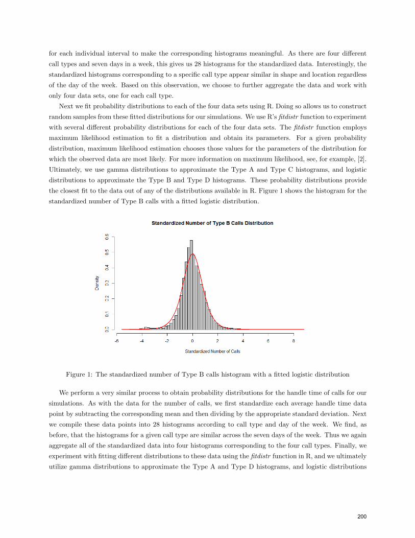
the closest fit to the data out of any of the distributions available in R. Figure 1 shows the histogram for the
standardized number of Type B calls with a fitted logistic distribution.
Figure 1: The standardized number of Type B calls histogram with a fitted logistic distribution
We perform a very similar process to obtain probability distributions for the handle time of calls for our
simulations. As with the data for the number of calls, we first standardize each average handle time data
point by subtracting the corresponding mean and then dividing by the appropriate standard deviation. Next
we compile these data points into 28 histograms according to call type and day of the week. We find, as
before, that the histograms for a given call type are similar across the seven days of the week. Thus we again
aggregate all of the standardized data into four histograms corresponding to the four call types. Finally, we
experiment with fitting different distributions to these data using the fitdistr function in R, and we ultimately
utilize gamma distributions to approximate the Type A and Type D histograms, and logistic distributions
200
to approximate the Type B and Type C histograms. Again, we choose these probability distributions not
based on precedents in the literature, but because they give the best fit to the data of any of the distributions
available in R. Table 1 in Appendix A displays the estimated gamma and logistic parameters corresponding
to the fitted number of call and handle time distributions.
The only other data we need for the simulations is the time between each call. Unfortunately, Nationwide’s
data set provides no information on this particular quantity. However, it is common in the literature on call
center modeling to assume that call arrivals form a Poisson process, and hence that the time between phone
calls follows an exponential distribution (see, e.g. [5]). Thus we obtain the time between calls for each 30-
minute interval corresponding to a particular call type and day of the week by sampling from an exponential
distribution based on the average number of calls in that interval (as calculated from the Nationwide data
set).
The process of generating random samples from the appropriate distributions for a given simulation is
fairly simple in R. For each 30-minute interval of the workday corresponding to a particular call type and
day of the week, we generate both the number of calls and the handle time of each call using R’s rgamma and
rlogis functions with the parameters of the corresponding fitted distributions. In order to put the random
data generated from these standardized distributions into the correct units for the simulations, we multiply
each data point by the appropriate standard deviation, add the appropriate mean, and round the resulting
number to the nearest integer (we assume that the number of calls and the handle time of each call are
integer variables). We generate data for the time between calls using an exponential distribution with the
appropriate parameter (as outlined in the previous paragraph), and we round the resulting numbers to the
nearest integer. Finally, we output the randomly generated data for the number of calls, the handle time
of each call, and the time between each call to files so that the data can be read from these files into the
simulations.
4 Results
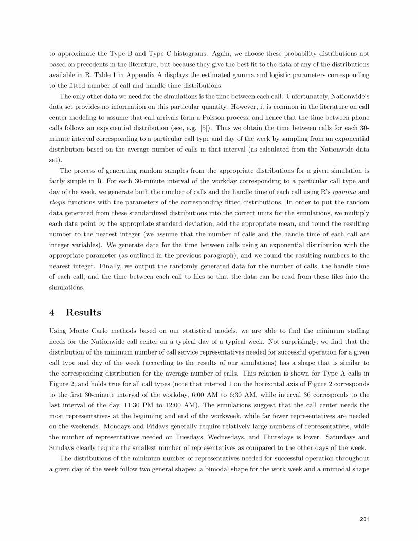
Using Monte Carlo methods based on our statistical models, we are able to find the minimum staffing
needs for the Nationwide call center on a typical day of a typical week. Not surprisingly, we find that the
distribution of the minimum number of call service representatives needed for successful operation for a given
call type and day of the week (according to the results of our simulations) has a shape that is similar to
the corresponding distribution for the average number of calls. This relation is shown for Type A calls in
Figure 2, and holds true for all call types (note that interval 1 on the horizontal axis of Figure 2 corresponds
to the first 30-minute interval of the workday, 6:00 AM to 6:30 AM, while interval 36 corresponds to the
last interval of the day, 11:30 PM to 12:00 AM). The simulations suggest that the call center needs the
most representatives at the beginning and end of the workweek, while far fewer representatives are needed
on the weekends. Mondays and Fridays generally require relatively large numbers of representatives, while
the number of representatives needed on Tuesdays, Wednesdays, and Thursdays is lower. Saturdays and
Sundays clearly require the smallest number of representatives as compared to the other days of the week.
The distributions of the minimum number of representatives needed for successful operation throughout
a given day of the week follow two general shapes: a bimodal shape for the work week and a unimodal shape
201
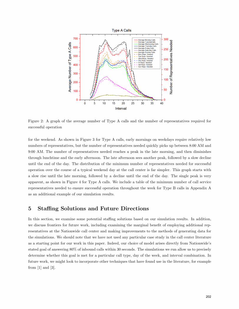
Figure 2: A graph of the average number of Type A calls and the number of representatives required for
successful operation
for the weekend. As shown in Figure 3 for Type A calls, early mornings on weekdays require relatively low
numbers of representatives, but the number of representatives needed quickly picks up between 8:00 AM and
9:00 AM. The number of representatives needed reaches a peak in the late morning, and then diminishes
through lunchtime and the early afternoon. The late afternoon sees another peak, followed by a slow decline
until the end of the day. The distribution of the minimum number of representatives needed for successful
operation over the course of a typical weekend day at the call center is far simpler. This graph starts with
a slow rise until the late morning, followed by a decline until the end of the day. The single peak is very
apparent, as shown in Figure 4 for Type A calls. We include a table of the minimum number of call service
representatives needed to ensure successful operation throughout the week for Type B calls in Appendix A
as an additional example of our simulation results.
5 Staffing Solutions and Future Directions
In this section, we examine some potential staffing solutions based on our simulation results. In addition,
we discuss frontiers for future work, including examining the marginal benefit of employing additional rep-
resentatives at the Nationwide call center and making improvements to the methods of generating data for
the simulations. We should note that we have not used any particular case study in the call center literature
as a starting point for our work in this paper. Indeed, our choice of model arises directly from Nationwide’s
stated goal of answering 80% of inbound calls within 30 seconds. The simulations we run allow us to precisely
determine whether this goal is met for a particular call type, day of the week, and interval combination. In
future work, we might look to incorporate other techniques that have found use in the literature, for example
from [1] and [3].
202
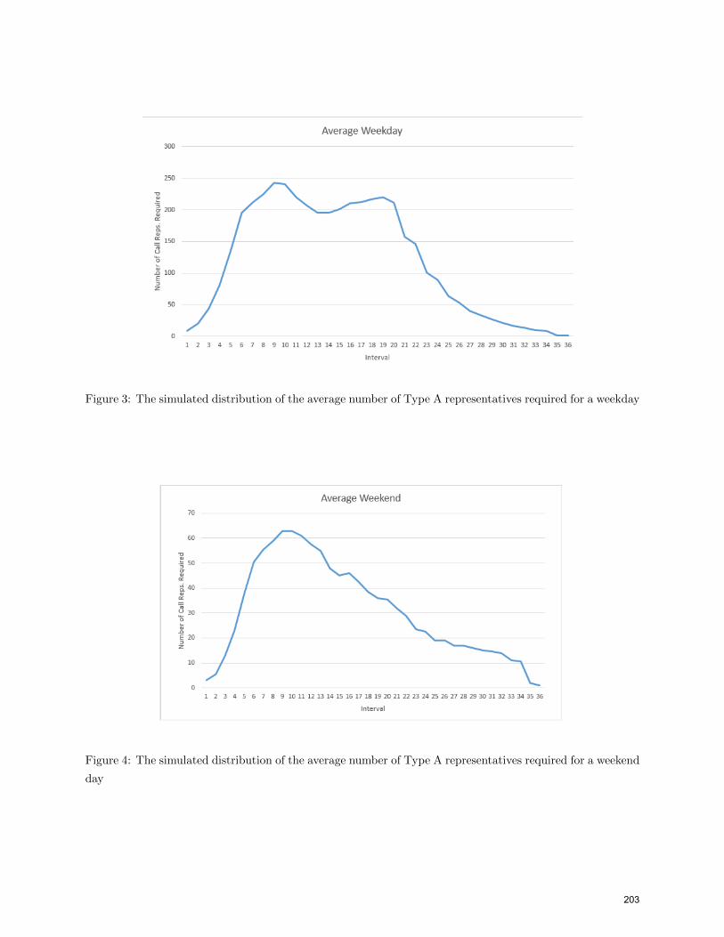
Figure 3: The simulated distribution of the average number of Type A representatives required for a weekday
Figure 4: The simulated distribution of the average number of Type A representatives required for a weekend
day
203
5.1 Staffing Solutions
Having acquired information regarding the staffing needs of the Nationwide call center via simulation, we
analyze different staffing plans, paying particular attention to the length and timing of shifts. The premise
for this work is that an existing call center employs a staffing system involving two nine-hour shifts: one from
6:00 AM to 3:00 PM, and the other from 3:00 PM until midnight. The results of our simulations suggest that
this staffing plan is not optimal, as the number of representatives needed for each call type varies drastically
(often by orders of magnitude) throughout the course of a given day.
We focus here on an algorithmic approach to developing a viable staffing plan that might produce an
improvement over the existing staffing plan. We devise and implement (via C++) an algorithm that attempts
to iteratively minimize the discrepancy between the number of call service representatives required to assure
successful operation for a given call type, day of the week, and interval combination (as prescribed by our
simulations) and the actual number of representatives on staff for that interval subject to restrictions on
shift length. We experiment with both the objective function that we seek to minimize and the constraint
of assumed shift lengths. We explore two particular objective functions: the sum of the absolute differences
between the ideal number of call service representatives and the actual number on staff, and the sum of the
squared differences between these two quantities (in the spirit of least squares regression). We implement
the algorithm subject to shift lengths of two hours up to shift lengths of ten hours (in integer increments).
We note here that we have explored modifications of the algorithm in which shift lengths are allowed to vary
in order to minimize the aforementioned criteria; however, for the purposes of this work, we assume each
employee has the same shift length.
As an example, we obtain the results in Figure 5 by implementing the algorithm under the assumption
that each call service representative works a two-hour shift and that the objective function is the sum of the
squared differences. The blue curve represents the ideal number of representatives that we obtain from our
simulations, while the orange curve represents the actual number of representatives on staff as recommended
by the algorithm. This graph is for Type B calls on Wednesday. We see that the orange curve is fairly close
to the blue curve for most of the day, but that there are some clear deviations between the two curves. The
program creates a staffing plan whereby representatives come to work on a rolling basis for each half-hour
interval, in contrast to the rigid system in which all employees work one of two possible shifts on a given
day.
A brute force search that guarantees a global minimum for the selected shift lengths and objective
function would be computationally expensive; we instead implement an iterative algorithm that runs until
the shifts appear to stabilize. Typically, proposed staffing numbers stabilize after about four iterations; we
therefore choose to run 10 iterations for each day. From experimentation, it appears that the sum of squared
differences objective function gives the best results; all further discussion pertains to the use of this objective
function.
While this staffing algorithm is not guaranteed to produce a global minimum, preliminary results of
applying the algorithm are promising. First and foremost, the algorithm does a much better job of staffing
than we are generally able to do manually (by trial and error). Indeed, when we graph the number of
representatives suggested by our algorithm for a given call type and day against the number of representatives
204
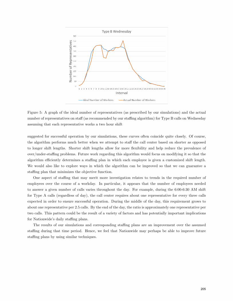
Figure 5: A graph of the ideal number of representatives (as prescribed by our simulations) and the actual
number of representatives on staff (as recommended by our staffing algorithm) for Type B calls on Wednesday
assuming that each representative works a two hour shift
suggested for successful operation by our simulations, these curves often coincide quite closely. Of course,
the algorithm performs much better when we attempt to staff the call center based on shorter as opposed
to longer shift lengths. Shorter shift lengths allow for more flexibility and help reduce the prevalence of
over/under-staffing problems. Future work regarding this algorithm would focus on modifying it so that the
algorithm efficiently determines a staffing plan in which each employee is given a customized shift length.
We would also like to explore ways in which the algorithm can be improved so that we can guarantee a
staffing plan that minimizes the objective function.
One aspect of staffing that may merit more investigation relates to trends in the required number of
employees over the course of a workday. In particular, it appears that the number of employees needed
to answer a given number of calls varies throughout the day. For example, during the 6:00-6:30 AM shift
for Type A calls (regardless of day), the call center requires about one representative for every three calls
expected in order to ensure successful operation. During the middle of the day, this requirement grows to
about one representative per 2.5 calls. By the end of the day, the ratio is approximately one representative per
two calls. This pattern could be the result of a variety of factors and has potentially important implications
for Nationwide’s daily staffing plans.
The results of our simulations and corresponding staffing plans are an improvement over the assumed
staffing during that time period. Hence, we feel that Nationwide may perhaps be able to improve future
staffing plans by using similar techniques.
205
5.2 Marginal Benefit of Additional Representatives
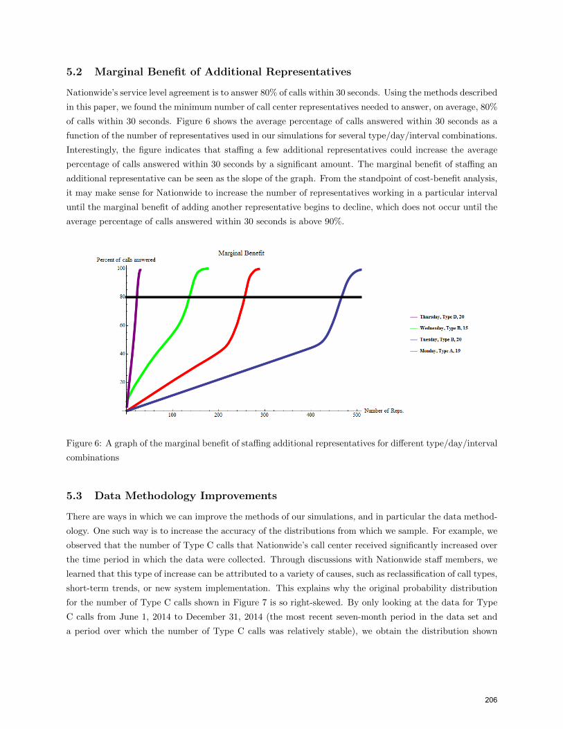
Nationwide’s service level agreement is to answer 80% of calls within 30 seconds. Using the methods described
in this paper, we found the minimum number of call center representatives needed to answer, on average, 80%
of calls within 30 seconds. Figure 6 shows the average percentage of calls answered within 30 seconds as a
function of the number of representatives used in our simulations for several type/day/interval combinations.
Interestingly, the figure indicates that staffing a few additional representatives could increase the average
percentage of calls answered within 30 seconds by a significant amount. The marginal benefit of staffing an
additional representative can be seen as the slope of the graph. From the standpoint of cost-benefit analysis,
it may make sense for Nationwide to increase the number of representatives working in a particular interval
until the marginal benefit of adding another representative begins to decline, which does not occur until the
average percentage of calls answered within 30 seconds is above 90%.
Figure 6: A graph of the marginal benefit of staffing additional representatives for different type/day/interval
combinations
5.3 Data Methodology Improvements
There are ways in which we can improve the methods of our simulations, and in particular the data method-
ology. One such way is to increase the accuracy of the distributions from which we sample. For example, we
observed that the number of Type C calls that Nationwide’s call center received significantly increased over
the time period in which the data were collected. Through discussions with Nationwide staff members, we
learned that this type of increase can be attributed to a variety of causes, such as reclassification of call types,
short-term trends, or new system implementation. This explains why the original probability distribution
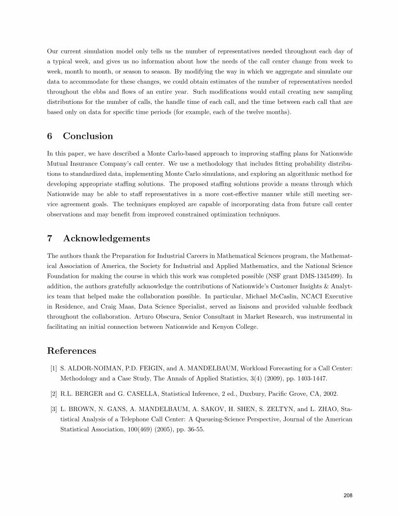
for the number of Type C calls shown in Figure 7 is so right-skewed. By only looking at the data for Type
C calls from June 1, 2014 to December 31, 2014 (the most recent seven-month period in the data set and
a period over which the number of Type C calls was relatively stable), we obtain the distribution shown
206
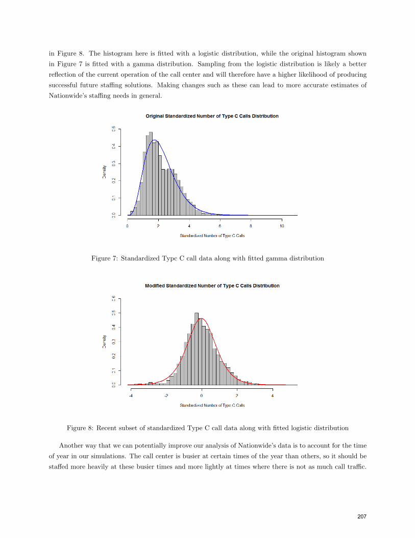
in Figure 8. The histogram here is fitted with a logistic distribution, while the original histogram shown
in Figure 7 is fitted with a gamma distribution. Sampling from the logistic distribution is likely a better
reflection of the current operation of the call center and will therefore have a higher likelihood of producing
successful future staffing solutions. Making changes such as these can lead to more accurate estimates of
Nationwide’s staffing needs in general.
Figure 7: Standardized Typc C call data along with fitted gamma distribution
Figure 8: Recent subset of standardized Type C call data along with fitted logistic distribution
Another way that we can potentially improve our analysis of Nationwide’s data is to account for the time
of year in our simulations. The call center is busier at certain times of the year than others, so it should be
staffed more heavily at these busier times and more lightly at times where there is not as much call traffic.
207
Our current simulation model only tells us the number of representatives needed throughout each day of
a typical week, and gives us no information about how the needs of the call center change from week to
week, month to month, or season to season. By modifying the way in which we aggregate and simulate our
data to accommodate for these changes, we could obtain estimates of the number of representatives needed
throughout the ebbs and flows of an entire year. Such modifications would entail creating new sampling
distributions for the number of calls, the handle time of each call, and the time between each call that are
based only on data for specific time periods (for example, each of the twelve months).
6 Conclusion
In this paper, we have described a Monte Carlo-based approach to improving staffing plans for Nationwide
Mutual Insurance Company’s call center. We use a methodology that includes fitting probability distribu-
tions to standardized data, implementing Monte Carlo simulations, and exploring an algorithmic method for
developing appropriate staffing solutions. The proposed staffing solutions provide a means through which
Nationwide may be able to staff representatives in a more cost-effective manner while still meeting ser-
vice agreement goals. The techniques employed are capable of incorporating data from future call center
observations and may benefit from improved constrained optimization techniques.
7 Acknowledgements
The authors thank the Preparation for Industrial Careers in Mathematical Sciences program, the Mathemat-
ical Association of America, the Society for Industrial and Applied Mathematics, and the National Science
Foundation for making the course in which this work was completed possible (NSF grant DMS-1345499). In
addition, the authors gratefully acknowledge the contributions of Nationwide’s Customer Insights & Analyt-
ics team that helped make the collaboration possible. In particular, Michael McCaslin, NCACI Executive
in Residence, and Craig Maas, Data Science Specialist, served as liaisons and provided valuable feedback
throughout the collaboration. Arturo Obscura, Senior Consultant in Market Research, was instrumental in
facilitating an initial connection between Nationwide and Kenyon College.
References
[1] S. ALDOR-NOIMAN, P.D. FEIGIN, and A. MANDELBAUM, Workload Forecasting for a Call Center:
Methodology and a Case Study, The Annals of Applied Statistics, 3(4) (2009), pp. 1403-1447.
[2] R.L. BERGER and G. CASELLA, Statistical Inference, 2 ed., Duxbury, Pacific Grove, CA, 2002.
[3] L. BROWN, N. GANS, A. MANDELBAUM, A. SAKOV, H. SHEN, S. ZELTYN, and L. ZHAO, Sta-
tistical Analysis of a Telephone Call Center: A Queueing-Science Perspective, Journal of the American
Statistical Association, 100(469) (2005), pp. 36-55.
208
[4] W. FOX, F. GIORDANO, S. HORTON, and M. WEIR, A First Course in Mathematical Modeling, 4
ed., Cengage Learning, Belmont, CA, 2008.
[5] N. GANS, G. KOOLE, and A. MANDELBAUM, Telephone Call Centers: Tutorial, Review, and Re-
search Prospects, Manufacturing & Service Operations Management, 5(2) (2003), pp. 79-141.
[6] D.S. MALIK, Data Structures Using C++, 2 ed., Cengage Learning, Boston, MA, 2009.
[7] Nationwide and Affiliated Companies. Retrieved 18 June 2015 from http://www.nationwide.com/about-
us/affiliated-companies.jsp.
[8] R Core Team (2013). R: A language and environment for statistical computing. R Foundation for
Statistical Computing, Vienna, Austria. URL http://www.R-project.org/.
209
Appendix A
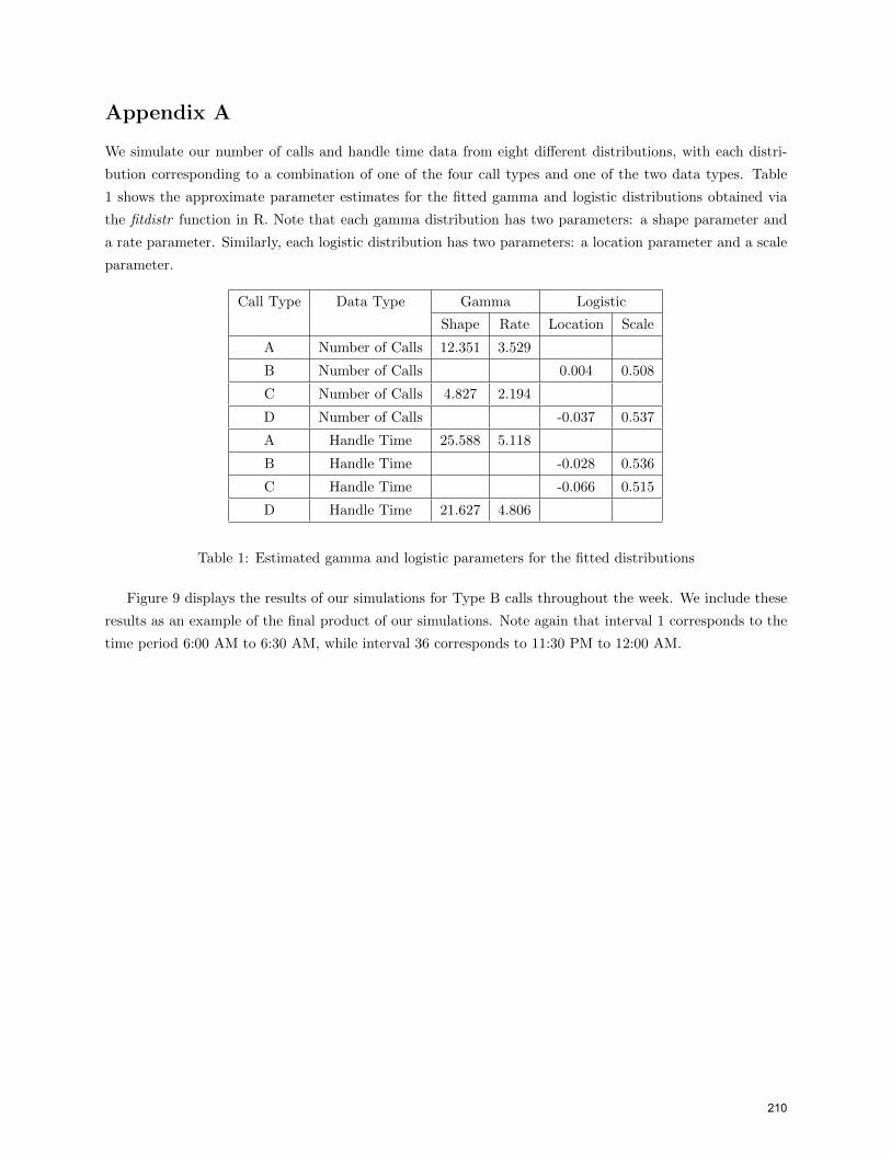
We simulate our number of calls and handle time data from eight different distributions, with each distri-
bution corresponding to a combination of one of the four call types and one of the two data types. Table
1 shows the approximate parameter estimates for the fitted gamma and logistic distributions obtained via
the fitdistr function in R. Note that each gamma distribution has two parameters: a shape parameter and
a rate parameter. Similarly, each logistic distribution has two parameters: a location parameter and a scale
parameter.
Call Type Data Type Gamma Logistic
Shape Rate Location Scale
A Number of Calls 12.351 3.529
B Number of Calls 0.004 0.508
C Number of Calls 4.827 2.194
D Number of Calls -0.037 0.537
A Handle Time 25.588 5.118
B Handle Time -0.028 0.536
C Handle Time -0.066 0.515
D Handle Time 21.627 4.806
Table 1: Estimated gamma and logistic parameters for the fitted distributions
Figure 9 displays the results of our simulations for Type B calls throughout the week. We include these
results as an example of the final product of our simulations. Note again that interval 1 corresponds to the
time period 6:00 AM to 6:30 AM, while interval 36 corresponds to 11:30 PM to 12:00 AM.
210
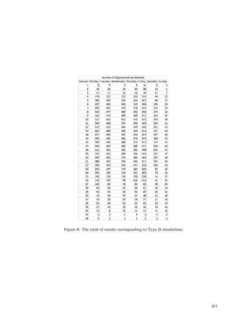
Figure 9: The table of results corresponding to Type B simulations
211