Optimal Borrowing Constraints and Growth

in a Small Open Economy

Amanda Michaud Jacek Rothert∗

Indiana University U.S. Naval Academy

March 4, 2014

Abstract

Chinese high growth has been accompanied by government restrictions on inter-

national borrowing (capital controls). In this paper, we ask: are such restrictions a

useful policy tool to facilitate growth? We provide a theory of borrowing constraints on

households as a tool to correct a learning-by-doing externality. Borrowing constraints

operate as a policy tool through two channels: (i) increasing labor supply and (ii)

reallocating labor towards traded goods. We find welfare gains are closest to that of

the Pareto efficient allocation when the externality is not too big or too small. We

compute the sequence of optimal constraints along the growth path and measure their

contribution to repressed wages, the current account, and real exchange rate underval-

uation.

Keywords: learning-by-doing, borrowing constraints, Chinese economy

∗Corresponding author; E-mail: jacek.rothert@gmail.com; Phone: (1)-410-293-5379;

Mailing address:

Department of Economics, United States Naval Academy; 589 McNair Rd, Annapolis, MD 21402

1

1 Introduction

Financial liberalizations of the late 1980’s and 1990’s came on the heels of economic literature

linking underdeveloped financial markets to poor economic outcomes.1 China has followed

a different path. For several decades Chinese policy repressed financial markets while the

country experienced extraordinary economic growth. As the world seeks to take a lesson from

the Chinese experience, important questions remain unsolved. Did China grow in spite of

these policies, or can financial repression promote growth? If the latter is true and financial

repression can increase growth, is it at the cost or the benefit to the welfare of households?

Our goal is to address these questions by better understanding financially repressive polices

as a tool to facilitate growth.

We provide a theory of borrowing constraints on households as a means to facilitate

growth through a “learning-by-doing” (LBD) externality (Arrow (1962), Romer (1986)).

LBD is the idea that increased production accelerates productivity growth through institu-

tional learning. The mechanism is straightforward. Borrowing constraints have a negative

wealth effect on households.2 If leisure is a normal good, poorer households consume less

leisure and work more. The LBD externality translates higher labor today into higher growth

by increasing future productivity. Thus, borrowing constraints facilitate growth.

What is not obvious is how borrowing constraints affect welfare. Our main finding is

optimal borrowing constraints produce outcomes closest to Pareto efficiency for values of the

learning-by-doing externality that are not too large or too small. This result is explained as

follows. Correcting a large learning by doing externality implies a large increase in permanent

income. However, if borrowing constraints are used to correct the externality, households will

be limited in smoothing consumption. Therefore, households enjoy a smaller share of the

welfare gains from correcting the externality when LBD is large. For smaller values of LBD,

the increase in permanent income is smaller, and the contemporaneous increase in output

1Financial reforms were one part of a general package of market-based reforms prescribed to developing

countries by the IMF, World Bank, and US Treasury during this time. This broad-based unanimity of this

view in these international institutions is referred to as the Washington Consensus.2Technically, total wealth is unchanged, but the availability of wealth in a given period is constrained.

2

from higher labor supply today is sufficient to smooth consumption without borrowing.

Therefore households enjoy a large share of the welfare gains from correcting the externality

when LBD is moderate-sized.

We provide a quantitative example to explore our theory in the context of the Chinese

growth experience. We consider a two-sector model of traded (manufacturing) and non-

traded goods, where LBD occurs in the traded sector. We calibrate the model to the Chinese

economy from 1990-2009, considering several LBD elasticities and choosing a sequence of

borrowing constraints to match the time series of differences between average Chinese and

US real GDP per capita growth. First, we find the elasticity of substitution between traded

and non-traded goods is the most important determinate of whether the policy is welfare

improving. Second, the quantitative experiment provides evidence the mechanics at work

in our model are supported by the data. The model with borrowing constraints provides

annual real wage growth, current account balance, and ending net foreign asset position of

magnitudes significantly closer to the data than implied by the laissez faire allocation.

Optimal, government-imposed borrowing constraints on households are one of several

second-best policy tools, so why are we studying them? First, we observe these policies in

practice3. Second, alternative first-best and second-best tools may be unavailable. Pigovian

taxes can achieve the first-best in theory, but are unlikely to be perfectly implementable. This

is because: (i) difficulties implementing subsidies specifically targeted at sources of growth

externalities; (ii) WTO regulations may preclude uses in tradeable sectors; and (iii) non-

distortionary (lump-sum) taxes/transfers necessary to achieve the first best are unrealistic.

Capital controls, exchange rate, and monetary policy are all second-best instruments in our

framework. We do not claim that all other tools are off the table, but acknowledge the

practicality of any one tool may be limited by changing circumstances. Although these

tools may interact, we analyze capital controls in isolation to provide clear insight into the

mechanism. We learn under what circumstances capital controls capture the largest share of

available welfare gains and conclude these are the circumstances where capital controls are

most useful relative to other second-best policies.

3See Ostry et al. (2010) for empirical analysis on the incidence and outcomes of different regulations to

manipulate capital flows.

3

Related Literature The use of welfare improving capital controls to correct externalities

is an area of active research.4 Recent literature mainly focuses on prudential controls to

regulate pecuniary externalities from over-borrowing.5 Another application is regulating the

interaction between private credit markets and sovereign debt markets.6 We focus instead on

growth externalities, similar to the ones studied in Costinot et al. (2011). Our contribution

is (i) an analytic and quantitative study of the effects of capital controls on labor supply and

allocation across sectors; and (ii) we compute the entire time path of the optimal policy, in

the Ramsey sense, both on and off equilibrium path.

Our work belongs to the literature in which financial repression fosters growth. The mech-

anism typically analyzed is how financial repression increases savings rates providing higher

capital investment to firms (Jappelli and Pagano (1994), Castro et al. (2004))7. In contrast,

we consider financial repression also generates a negative income effect on households which

increases labor supply to firms.

We integrate our work with the previous literature by incorporating the channel of sub-

stitution studied in Deaton and Laroque (1999). They show the laissez-faire allocation is

inefficient if assets in one sector (manufacturing) contribute to growth while assets in other

sectors (agriculture or construction) do not. Policies reallocating resources to sectors with

the learning-by-doing externality can then improve welfare. We model this channel using a

two sector model where the growth externality is higher in traded than non-traded sectors.

We then decompose the effect of the borrowing constraint into an increase in labor from the

income effect and a reallocation of labor across sectors.

A difference between our work and Deaton and Laroque (1999) and Jappelli and Pagano

(1994) is that we consider an open economy. This connects us to the literature on learning-

by-doing and the current account. Korinek and Serven (2010) show real exchange rate

(RER) undervaluation can correct the learning-by-doing externality. Aizenman and Lee

(2010) show undervaluation of RER will improve welfare only if learning-by-doing occurs

4See Farhi and Werning (2012) and Korinek (2011) for overviews of applications.5Including Schmitt-Grohe and Uribe (2012), Benigno et al. (2013) and Bianchi (2011) in two-sector small

open economies similar to our environment.6Wright (2006), Jeske (2006), Dovis (2012)7See Pagano (1993) for an early discussion of the two competing effects of financial repression.

4

through increased employment (rather than higher capital stock). Our paper adds to this

literature by considering elastic labor supply and by developing a non-monetary policy tool.

Like several other papers on current account surpluses in East Asia,8 we focus on credit

market imperfections. Unlike previous literature we consider government imposed restric-

tions on household borrowing. This is different from Buera and Shin (2009) or Song et al.

(2011) in that we focus on households rather than firms. It is also different from Mendoza

et al. (2009) or Carroll and Jeanne (2009) in that we consider government imposed re-

strictions, rather than exogenous “credit market imperfections” or “underdeveloped banking

sectors”.

The empirical literature provides evidence the learning-by-doing externality we consider

may be significant.9 These estimates depend on where one is looking for the externality. Esti-

mates for industrial sectors and learning-by-exporting are generally significant(Harrison and

Rodriguez-Clare (2009), Rodrik (2008)). Empirical studies of China, the country motivating

our work, also find strong evidence for these externalities, (Jarreau and Poncet (2009) and

Du et al. (2012)). The inconclusiveness of this literature precisely motivates our theoretical

study to provide additional testable implications to guide empirical efforts.

2 Theory

We break the model apart to clarify the economics behind each mechanism. We use a one-

sector model with elastic labor supply to isolate the income effect borrowing constraints

have on labor supply. We then use a two-sector model with inelastic labor supply to isolate

the reallocation effect borrowing constraints have in moving labor from non-tradeables to

tradeables.

8See Gourinchas and Jeanne (2013) for the empirical analysis.9Giles and Williams (2001a) and Giles and Williams (2001b) provide a literature review.

5

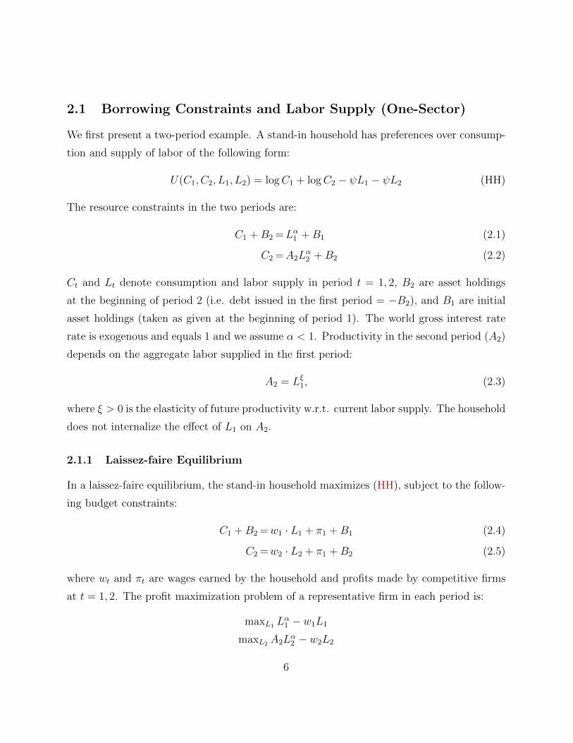
2.1 Borrowing Constraints and Labor Supply (One-Sector)

We first present a two-period example. A stand-in household has preferences over consump-

tion and supply of labor of the following form:

U(C1, C2, L1, L2) = logC1 + logC2 − ψL1 − ψL2 (HH)

The resource constraints in the two periods are:

C1 +B2 =Lα1 +B1 (2.1)

C2 =A2Lα2 +B2 (2.2)

Ct and Lt denote consumption and labor supply in period t = 1, 2, B2 are asset holdings

at the beginning of period 2 (i.e. debt issued in the first period = −B2), and B1 are initial

asset holdings (taken as given at the beginning of period 1). The world gross interest rate

rate is exogenous and equals 1 and we assume α < 1. Productivity in the second period (A2)

depends on the aggregate labor supplied in the first period:

A2 = Lξ1, (2.3)

where ξ > 0 is the elasticity of future productivity w.r.t. current labor supply. The household

does not internalize the effect of L1 on A2.

2.1.1 Laissez-faire Equilibrium

In a laissez-faire equilibrium, the stand-in household maximizes (HH), subject to the follow-

ing budget constraints:

C1 +B2 =w1 · L1 + π1 +B1 (2.4)

C2 =w2 · L2 + π1 +B2 (2.5)

where wt and πt are wages earned by the household and profits made by competitive firms

at t = 1, 2. The profit maximization problem of a representative firm in each period is:

maxL1 Lα1 − w1L1

maxL2 A2Lα2 − w2L2

6

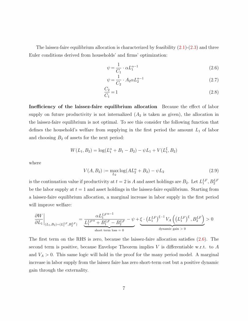
The laissez-faire equilibrium allocation is characterized by feasibility (2.1)-(2.3) and three

Euler conditions derived from households’ and firms’ optimization:

ψ=1

C1

· αLα−11 (2.6)

ψ=1

C2

· A2αLα−12 (2.7)

C2

C1

= 1 (2.8)

Inefficiency of the laissez-faire equilibrium allocation Because the effect of labor

supply on future productivity is not internalized (A2 is taken as given), the allocation in

the laissez-faire equilibrium is not optimal. To see this consider the following function that

defines the household’s welfare from supplying in the first period the amount L1 of labor

and choosing B2 of assets for the next period:

W (L1, B2) = log(Lα1 +B1 −B2)− ψL1 + V (Lξ1, B2)

where

V (A,B2) := maxL2

log(ALα2 +B2)− ψL2 (2.9)

is the continuation value if productivity at t = 2 is A and asset holdings are B2. Let LLF1 , BLF2

be the labor supply at t = 1 and asset holdings in the laissez-faire equilibrium. Starting from

a laissez-faire equilibrium allocation, a marginal increase in labor supply in the first period

will improve welfare:

∂W

∂L1

∣∣∣∣(L1,B2)=(LLF1 ,BLF2 )

=αLLF1

α−1

LLF1α

+BLF1 −BLF

2

− ψ︸ ︷︷ ︸short term loss = 0

+ ξ ·(LLF1

)ξ−1VA

((LLF1

)ξ, BLF

2

)︸ ︷︷ ︸

dynamic gain > 0

> 0

The first term on the RHS is zero, because the laissez-faire allocation satisfies (2.6). The

second term is positive, because Envelope Theorem implies V is differentiable w.r.t. to A

and VA > 0. This same logic will hold in the proof for the many period model. A marginal

increase in labor supply from the laissez faire has zero short-term cost but a positive dynamic

gain through the externality.

7

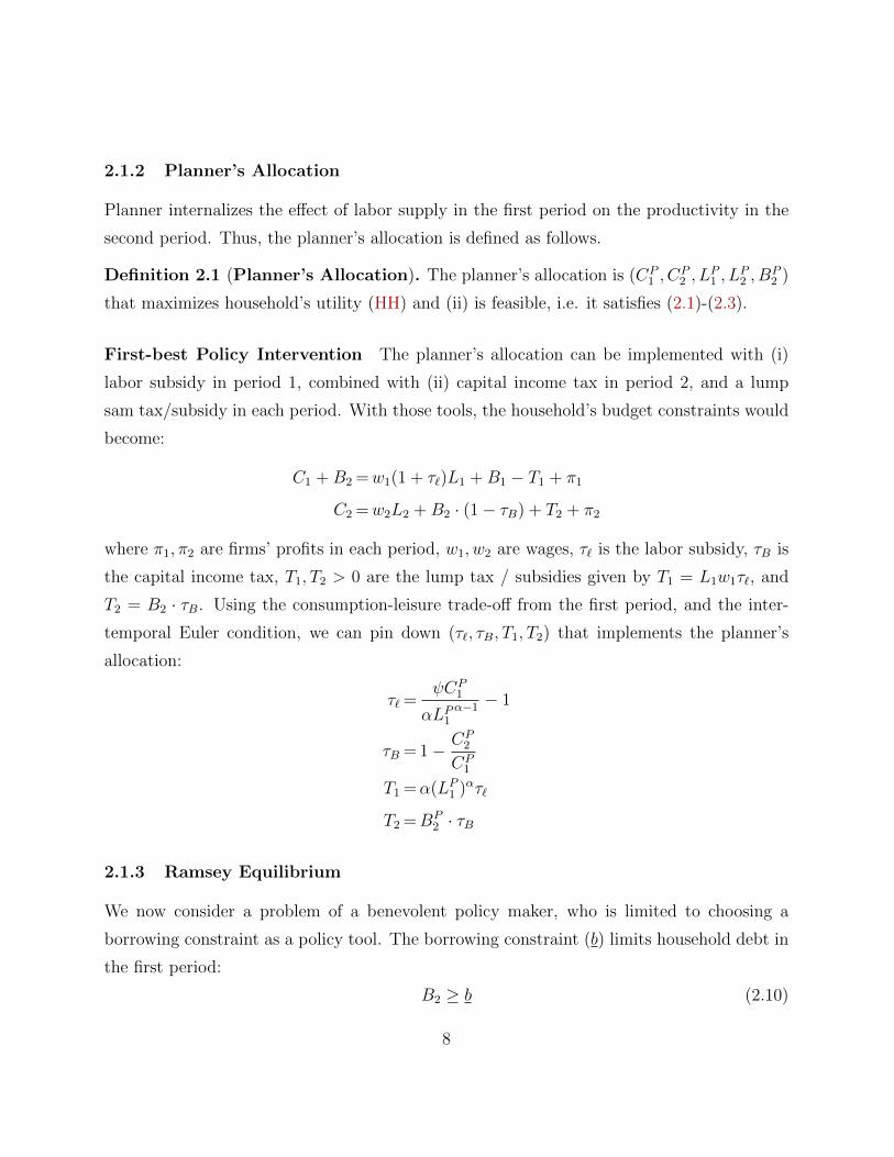
2.1.2 Planner’s Allocation

Planner internalizes the effect of labor supply in the first period on the productivity in the

second period. Thus, the planner’s allocation is defined as follows.

Definition 2.1 (Planner’s Allocation). The planner’s allocation is (CP1 , C

P2 , L

P1 , L

P2 , B

P2 )

that maximizes household’s utility (HH) and (ii) is feasible, i.e. it satisfies (2.1)-(2.3).

First-best Policy Intervention The planner’s allocation can be implemented with (i)

labor subsidy in period 1, combined with (ii) capital income tax in period 2, and a lump

sam tax/subsidy in each period. With those tools, the household’s budget constraints would

become:

C1 +B2 =w1(1 + τ`)L1 +B1 − T1 + π1

C2 =w2L2 +B2 · (1− τB) + T2 + π2

where π1, π2 are firms’ profits in each period, w1, w2 are wages, τ` is the labor subsidy, τB is

the capital income tax, T1, T2 > 0 are the lump tax / subsidies given by T1 = L1w1τ`, and

T2 = B2 · τB. Using the consumption-leisure trade-off from the first period, and the inter-

temporal Euler condition, we can pin down (τ`, τB, T1, T2) that implements the planner’s

allocation:

τ` =ψCP

1

αLP1α−1 − 1

τB = 1− CP2

CP1

T1 =α(LP1 )ατ`

T2 =BP2 · τB

2.1.3 Ramsey Equilibrium

We now consider a problem of a benevolent policy maker, who is limited to choosing a

borrowing constraint as a policy tool. The borrowing constraint (b) limits household debt in

the first period:

B2 ≥ b (2.10)

8

We define a borrowing-constrained allocation as follows.

Definition 2.2. A borrowing-constrained allocation is (Ct(b), Lt(b))t=1,2 that maximizes

(HH) subject to the resource constraints (2.1)-(2.2), the intra-temporal Euler Equation (2.6),

and the borrowing constraint (2.10).

In words, a borrowing-constrained allocation is the allocation that arises in a competitive

equilibrium, in which household faces the borrowing constraint (2.10).

Formally, the policy maker solves a Ramsey problem of the following form:

maxb

log(C1(b)) + log(C2(b))− ψL1((b))− ψL2(b)

where (Ct(b), Lt(b))t=1,2 is the borrowing-constrained allocation defined above. For a given

size of the LBD externality, the value of the borrowing-constrained allocation is given by:

W (b) = maxC1,L1,B2

log(C1)− ψL1 + V(Lξ1, B2

)(2.11)

subject to the resource constraint (2.1), the borrowing constraint (2.10) and household’s

endogenous reaction to the policy10. This is summarized by the Euler Equation (2.6), referred

to in this context as the implementability condition.

Definition 2.3 (Ramsey Equilibrium Allocation). The Ramsey Equilibrium Allocation

is (Ct(b∗), Lt(b

∗))t=1,2 with the borrowing constraint set to b∗ = arg maxbW (b).

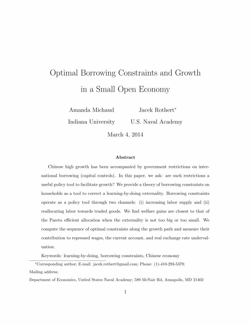
Proposition 2.1. The optimal borrowing constraint is unique, binds, and im-

proves welfare.

Let BLF2 be the asset holdings chosen in the laissez-faire allocation. There exists a unique

b∗ > B∗2 such that b∗ = arg maxbW (b), with W defined in (2.11).

Proof. In any equilibrium the intra-temporal Euler equation must hold. If leisure is a normal

good, then tighter borrowing constraint will raise the labor supply through income effect :

αLα−11

Lα1 +B1 − b− ψ = 0⇒ dL1

db> 0

10Households take the policy as given and do not internalize the effect of their behavior on the choice of

the policy maker

9

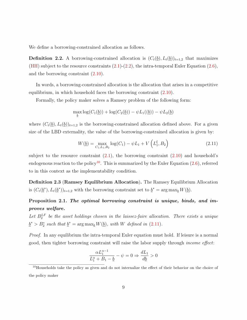
As a result, productivity and the continuation value in the second period increase. When

b = BLF2 , a marginal increase in b will have first-order effects only on the continuation

value. The proof of uniqueness exploits the non-monotone effect of the optimal constraint

on welfare. Very tight constraint (high b) will drive consumption down too much11. This is

illustrated in Figure 1.

B Laissez−FaireBorrowing constraint at t = 1

Val

ue o

f the

allo

catio

n

Constrained allocationLaissez−Faire allocation

Figure 1: Welfare in a borrowing-constrained allocation

Parameters: α = ψ = 0.67;B1 = 0.

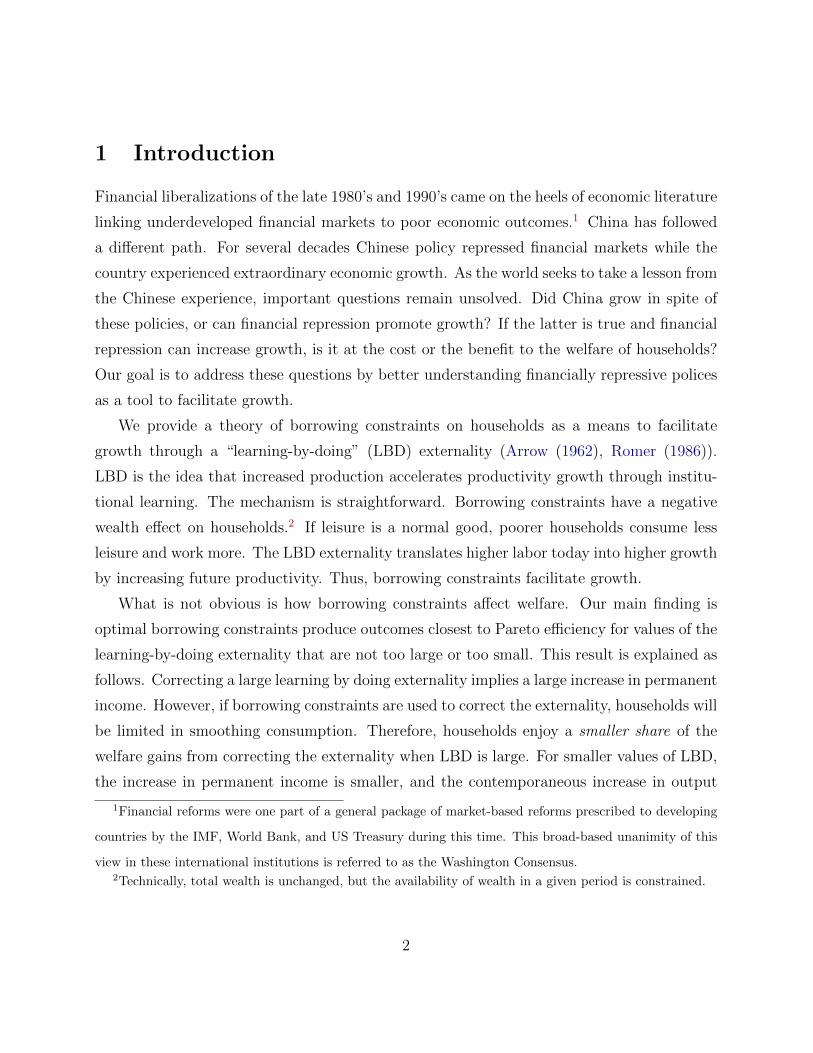
2.1.4 “Usefulness” of optimal borrowing constraints

We now turn to our next question: how useful a policy tool are borrowing constraints

in the world with learning-by-doing externalities? We address the qualitative aspect

of this question by comparing (i) the welfare gains from imposing optimal constraints to (ii)

welfare gains from moving to the planner’s allocation. Specifically, we explore how the size

11Formally, existence of an optimal constraint follows from the fact we are choosing b from [BLF2 ,∞) and

that limb→∞∂W∂b = −∞, which implies we can consider a truncation of [BLF

2 ,∞) and have W (a continuous

function) defined over a compact set.

10

of the externality affects the fraction of the planner’s welfare gains captured with optimally

chosen borrowing constraints.

When the size of the externality is ξ, the utility achieved in the planner’s allocation is:

V P (ξ) = maxL1,B2

log (Lα1 +B1 −B2)− ψL1 + V(Lξ1, B2

)where V is the continuation value defined in (2.9). Notice that no additional constraints are

imposed in the above maximization problem.

The value of the equilibrium allocation with optimal constraints is given by:

V OC(ξ) = maxbW (b; ξ)

where W (b; ξ) is defined in (2.11) on page 9. We measure welfare gains as the percent increase

in annual consumption over the laissez-faire equilibrium allocation necessary to achieve the

specified level of utility.

0 0.67

0.45

0.5

0.55

Usefulness of the optimal constraint

Size of externality (ξ)

Fra

ctio

n o

f P

lan

ner

’s w

elfa

re g

ain

s

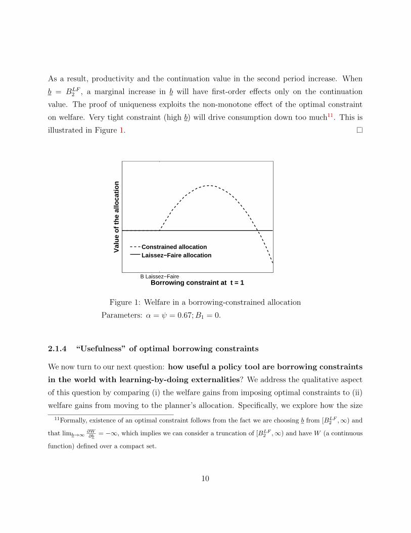
Figure 2: Size of externality and fraction of Planner’s welfare gains

Parameters: α = ψ = 0.67;B1 = 0.

The fraction of the welfare gain in Planner’s allocation (relative to laissez-faire) cap-

tured by the optimal borrowing constraint is depicted in Figure 2 for different values of

11

the externality. Two intuitive results emerge that hold in the many-period model: (1) the

Planner’s allocation always out-performs the optimal borrowing constraint allocation; and

(2) the optimal borrowing constraint achieves the largest fraction Planner’s welfare gain if

the LBD externality is neither too large, nor too small ( Figure 2). The intuition for this is

as follows. There is larger labor supply in both the Planner’s allocation and in the optimally

constrained allocation than in the laissez-faire allocation. This has two effects: first, current

income rises and second, permanent income rises. The Planner’s allocation takes advantage

of both effects, but the optimal constraints only take advantage of the first. Initially (small

LBD), an increase in the size of externality has a larger impact on current income relative

to permanent income, so the optimal constraint captures a larger and larger fraction of the

Planner’s welfare gains. For large values of the externality, the permanent income effect

starts to dominate. It then becomes optimal for the households to borrow to take advantage

of the increase in permanent income. The optimal borrowing constraint, by construction,

does not allow households to smooth consumption. An increasing fraction of the welfare

gain cannot be captured as the effect of the externality on permanent income increases.

−1 −0.5 0 0.5 10

0.05

0.1

0.15

0.2

0.25

B0 (initial assets)

% C

incr

ease

(P) Planner(OC) Optimal Constraint

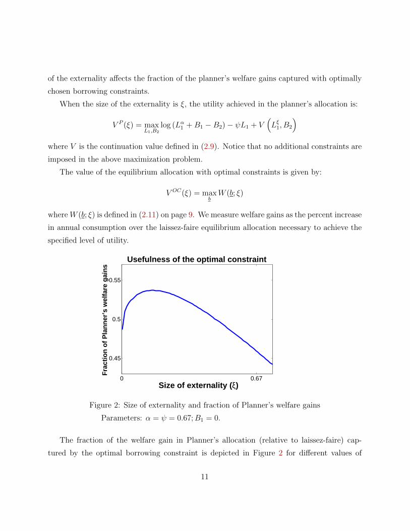
Figure 3: Size of initial assets and welfare gain

Parameters: α = ψ = 0.67; ξ = 0.05.

The initial asset position of the economy also determines the “usefulness” of the borrowing

12

constraint as a policy tool. Welfare gains of both the planner’s and Optimal Constraint

allocations are decreasing in the size of initial asset holdings ( Figure 3). This is intuitive,

because the benefit of the LBD externality is an increase wealth. Welfare gains fall for

wealthy agents if the marginal value of wealth is small relative to the cost of lost leisure.

As the welfare gain from the planner’s and Optimal Constraint each decrease, the Optimal

Constraint also captures less of the welfare gain of the planner’s allocation.

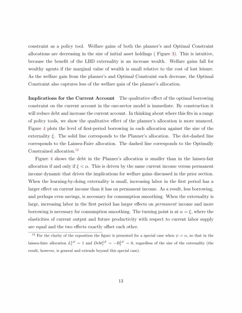
Implications for the Current Account The qualitative effect of the optimal borrowing

constraint on the current account in the one-sector model is immediate. By construction it

will reduce debt and increase the current account. In thinking about where this fits in a range

of policy tools, we show the qualitative effect of the planner’s allocation is more nuanced.

Figure 4 plots the level of first-period borrowing in each allocation against the size of the

externality ξ. The solid line corresponds to the Planner’s allocation. The dot-dashed line

corresponds to the Laissez-Faire allocation. The dashed line corresponds to the Optimally

Constrained allocation.12

Figure 4 shows the debt in the Planner’s allocation is smaller than in the laissez-fair

allocation if and only if ξ < α. This is driven by the same current income versus permanent

income dynamic that drives the implications for welfare gains discussed in the prior section.

When the learning-by-doing externality is small, increasing labor in the first period has a

larger effect on current income than it has on permanent income. As a result, less borrowing,

and perhaps even savings, is necessary for consumption smoothing. When the externality is

large, increasing labor in the first period has larger effects on permanent income and more

borrowing is necessary for consumption smoothing. The turning point is at α = ξ, where the

elasticities of current output and future productivity with respect to current labor supply

are equal and the two effects exactly offset each other.

12 For the clarity of the exposition the figure is presented for a special case when ψ = α, so that in the

laissez-faire allocation LLF1 = 1 and DebtLF

1 = −BLF2 = 0, regardless of the size of the externality (the

result, however, is general and extends beyond this special case).

13

0 0.67

0

Size of externality ( ξ)

Deb

t (−B

) / G

DP

at t

= 1

Borrowing at t = 1

(P) Planner(LF) Laissez−faire(OC) Optimal constraint

ξ = α

Figure 4: Size of externality and debt in the 2-period model

Parameters: α = ψ = 0.67;B1 = 0.

2.2 Infinite Horizon Quantitative Model

We now present the infinite-horizon model used for quantitative analysis of the one-sector

model. We continue to simplify the analysis using labor being the only factor of production,

but our results carry to a model with capital as shown in Section A.1 of the Appendix.

Households A stand-in household has preferences over consumption of a single tradable

good c and labor ` and maximizes the lifetime utility given by:

∞∑t=0

βtU(ct, `t) (2.12)

In each period t it faces the following sequence of budget constraints and debt limits:

ct + bt+1≤wt`t +R∗bt + πt (2.13)

bt+1≥ bt (2.14)

In the constraints above w denotes wage, b are bond holdings and π are firms’ profits. Our

assumption of a small open economy implies R∗ is exogenous (in our model it is constant:

14

R∗ = 1/β). We assume total labor is bounded ` ∈ [0, 1]. We allow for the debt limit in

(2.14) to be time varying, since we focus on the borrowing constraint as a policy tool that

may vary over time.

Firms The single consumption good is produced by competitive firms. A representative

firm chooses labor ` to maximize profits (π) subject to production technology F (·):

max`t

πt = AtF (`t)− wt`t

At is total factor productivity productivity, relative to the world frontier (which is normalized

to 1). Productivity next period depends on learning-by-doing technology φ(·):

At+1 = φ(At, `t)

The effect of today’s labor `t on tomorrow’s productivity At+1 is not internalized. In addi-

tion to standard regularity assumptions on utility and production, we assume the following

properties on the learning-by-doing technology:

Assumption 2.1. φ(At, `t) ∈ [At, 1] for all (At, `t); and φ`(At, `t) > 0 for every At ∈ (0, 1)

and every `t ∈ (0, 1).

Definition 2.4 (Equilibrium). Given initial productivity a0, bond holdings b0, and the se-

quence of debt limits (bt)∞t=0, an equilibrium consists of sequences of allocations (c∗t , `

∗t , b∗t+1)

∞t=0,

wages (w∗t )∞t=0, profits (π∗t )

∞t=0 and the sequence of productivity (a∗t+1)

∞t=0 such that, given the

wages and profits, (i) allocations solve the household’s and firms’ maximization problems

and (ii) markets clear.

As in the 2-period model, we focus on three allocations: (i) the Laissez-faire allocation,

which we treat as a benchmark, (ii) the Planner’s allocation, which is the first-best (opti-

mal) allocation, and (iii) the Ramsey Equilibrium allocation, which arises in a borrowing-

constrained equilibrium where a benevolent policy-maker chooses a sequence of borrowing

constraints that maximizes household’s welfare. We will start by defining and characterizing

each of these allocations in this ∞-horizon model.

15

2.2.1 Laissez-faire Equilibrium

Definition 2.5. A laissez-faire equilibrium is an equilibrium such that (2.14) never binds

(the Lagrange multiplier associated with (2.14) is 0 for every t).

Characterization The Laissez-faire Equilibrium Allocation solves the following dynamic

program:

V LF (A,B) = max{U(c, `) + βV LF (A′, B′)}

subject to:

A′= φ(c, `) (2.15)

c+B′=AF (`) +R∗B (2.16)

−U`(c, `) =Uc(c, `) · AF ′(`) (2.17)

Uc(c, `) = βR∗Uc(c′, `′) (2.18)

B′≥B (2.19)

where B is the natural borrowing limit. The first two constraints ensure the allocation is

feasible. The implementability conditions (2.17)-(2.18) ensure household’s first order con-

ditions are satisfied. The last condition is the no-Ponzi constraint. As was the case in the

two-period model, the laissez-faire allocation is inefficient, because the household does not

internalize the effect of labor supply on future productivity.

2.2.2 Planner’s Allocation

Definition 2.6 (Planner’s Allocation). The Planner’s allocation is a sequence (at+1, ct, `t, bt+1)∞t=0

that maximizes (3.1) subject to

At+1 = φ(At, `t), t = 0, 1, 2, ...∞∑t=0

ctR∗t≤∞∑t=0

atF (`t)

R∗t+R∗b0,

16

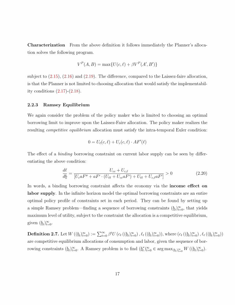
Characterization From the above definition it follows immediately the Planner’s alloca-

tion solves the following program.

V P (A,B) = max{U(c, `) + βV P (A′, B′)}

subject to (2.15), (2.16) and (2.19). The difference, compared to the Laissez-faire allocation,

is that the Planner is not limited to choosing allocation that would satisfy the implementabil-

ity conditions (2.17)-(2.18).

2.2.3 Ramsey Equilibrium

We again consider the problem of the policy maker who is limited to choosing an optimal

borrowing limit to improve upon the Laissez-Faire allocation. The policy maker realizes the

resulting competitive equilibrium allocation must satisfy the intra-temporal Euler condition:

0 = U`(c, `) + Uc(c, `) · AF ′(`)

The effect of a binding borrowing constraint on current labor supply can be seen by differ-

entiating the above condition:

d`

db=

Ucc + Uc,`[UcaF ′′ + aF ′ · (U`` + UccaF ′) + U`` + Uc,`aF ′]

> 0 (2.20)

In words, a binding borrowing constraint affects the economy via the income effect on

labor supply. In the infinite horizon model the optimal borrowing constraints are an entire

optimal policy profile of constraints set in each period. They can be found by setting up

a simple Ramsey problem—finding a sequence of borrowing constraints (bt)∞t=0, that yields

maximum level of utility, subject to the constraint the allocation is a competitive equilibrium,

given (bt)∞t=0.

Definition 2.7. LetW ((bt)∞t=0) :=

∑∞t=0 β

tU (ct ((bt)∞t=0) , `t ((bt)

∞t=0)), where (ct ((bt)

∞t=0) , `t ((bt)

∞t=0))

are competitive equilibrium allocations of consumption and labor, given the sequence of bor-

rowing constraints (bt)∞t=0. A Ramsey problem is to find (b∗t )

∞t=0 ∈ arg max(bt)

∞t=0W ((bt)

∞t=0).

17

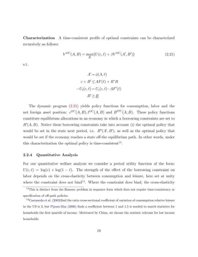
Characterization A time-consistent profile of optimal constraints can be characterized

recursively as follows:

V OC(A,B) = maxB{U(c, `) + βV OC(A′, B′)} (2.21)

s.t.

A′= φ(A, `)

c+B′≤AF (`) +R∗B

−U`(c, `) =Uc(c, `) · AF ′(`)

B′≥B

The dynamic program (2.21) yields policy functions for consumption, labor and the

net foreign asset position: cOC(A,B), `OC(A,B) and B′OC(A,B). These policy functions

constitute equilibrium allocations in an economy in which a borrowing constraints are set to

B′(A,B). Notice these borrowing constraints take into account (i) the optimal policy that

would be set in the state next period, i.e. B′′(A′, B′), as well as the optimal policy that

would be set if the economy reaches a state off-the equilibrium path. In other words, under

this characterization the optimal policy is time-consistent13.

2.2.4 Quantitative Analysis

For our quantitative welfare analysis we consider a period utility function of the form:

U(c, `) = log(c) + log(1 − `). The strength of the effect of the borrowing constraint on

labor depends on the cross-elasticity between consumption and leisure, here set at unity

where the constraint does not bind14. Where the constraint does bind, the cross-elasticity

13This is distinct from the Ramsey problem in sequence form which does not require time-consistency or

specification of off-path policies.14Castaneda et al. (2003)find the ratio cross-sectional coefficient of variation of consumption relative leisure

in the US is 3, but Pijoan-Mas (2006) finds a coefficient between 1 and 1.5 is needed to match statistics for

households the first quartile of income. Motivated by China, we choose the statistic relevant for low income

households.

18

between consumption and leisure will be higher.15

The production function is F (`) = `α. The learning-by-doing technology assumes con-

stant productivity catch-up:

a′ = min{1, a · eφ`} (2.22)

where φ measures the effect of ` on future productivity. We consider a range of values for

the learning-by-doing parameter: φ ∈ [0, 0.20]. We also consider how the results depend on

the initial level of productivity (relative to the world frontier). The remaining parameters

are set to standard values: β = 0.96, α = 0.67, R∗ = 1β. Initial assets are set to B0 = 0.

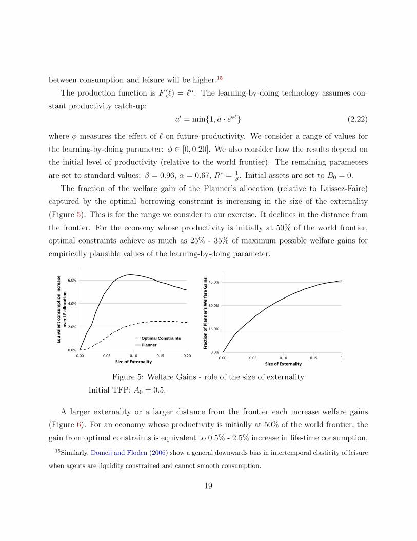
The fraction of the welfare gain of the Planner’s allocation (relative to Laissez-Faire)

captured by the optimal borrowing constraint is increasing in the size of the externality

(Figure 5). This is for the range we consider in our exercise. It declines in the distance from

the frontier. For the economy whose productivity is initially at 50% of the world frontier,

optimal constraints achieve as much as 25% - 35% of maximum possible welfare gains for

empirically plausible values of the learning-by-doing parameter.

0.0%

2.0%

4.0%

6.0%

0.00 0.05 0.10 0.15 0.20

Equ

ival

en

t co

nsu

mp

tio

n in

cre

ase

o

ver

LF a

lloca

tio

n

Size of Externality

Optimal Constraints

Planner

0.0%

15.0%

30.0%

45.0%

0.00 0.05 0.10 0.15 0.20

Frac

tio

n o

f P

lan

ne

r's

We

lfar

e G

ain

s

Size of Externality

Figure 5: Welfare Gains - role of the size of externality

Initial TFP: A0 = 0.5.

A larger externality or a larger distance from the frontier each increase welfare gains

(Figure 6). For an economy whose productivity is initially at 50% of the world frontier, the

gain from optimal constraints is equivalent to 0.5% - 2.5% increase in life-time consumption,

15Similarly, Domeij and Floden (2006) show a general downwards bias in intertemporal elasticity of leisure

when agents are liquidity constrained and cannot smooth consumption.

19

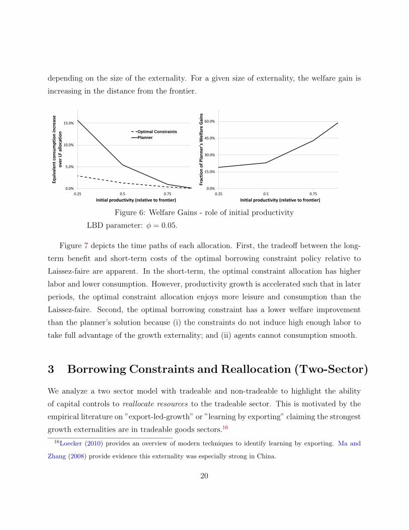
depending on the size of the externality. For a given size of externality, the welfare gain is

increasing in the distance from the frontier.

0.0%

5.0%

10.0%

15.0%

0.25 0.5 0.75

Equ

ival

en

t co

nsu

mp

tio

n in

cre

ase

o

ver

LF a

lloca

tio

n

Initial productivity (relative to frontier)

Optimal Constraints

Planner

0.0%

15.0%

30.0%

45.0%

60.0%

0.25 0.5 0.75

Frac

tio

n o

f P

lan

ne

r's

We

lfar

e G

ain

s Initial productivity (relative to frontier)

Figure 6: Welfare Gains - role of initial productivity

LBD parameter: φ = 0.05.

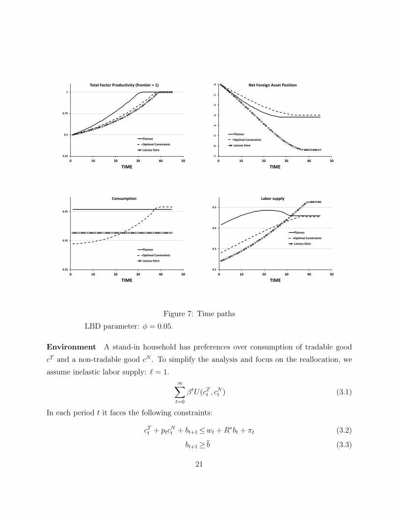
Figure 7 depicts the time paths of each allocation. First, the tradeoff between the long-

term benefit and short-term costs of the optimal borrowing constraint policy relative to

Laissez-faire are apparent. In the short-term, the optimal constraint allocation has higher

labor and lower consumption. However, productivity growth is accelerated such that in later

periods, the optimal constraint allocation enjoys more leisure and consumption than the

Laissez-faire. Second, the optimal borrowing constraint has a lower welfare improvement

than the planner’s solution because (i) the constraints do not induce high enough labor to

take full advantage of the growth externality; and (ii) agents cannot consumption smooth.

3 Borrowing Constraints and Reallocation (Two-Sector)

We analyze a two sector model with tradeable and non-tradeable to highlight the ability

of capital controls to reallocate resources to the tradeable sector. This is motivated by the

empirical literature on ”export-led-growth” or ”learning by exporting” claiming the strongest

growth externalities are in tradeable goods sectors.16

16Loecker (2010) provides an overview of modern techniques to identify learning by exporting. Ma and

Zhang (2008) provide evidence this externality was especially strong in China.

20

0.25

0.5

0.75

1

0 10 20 30 40 50

TIME

Total Factor Productivity (frontier = 1)

Planner

Optimal Constraints

Laissez-faire

-7

-6

-5

-4

-3

-2

-1

0

0 10 20 30 40 50

TIME

Net Foreign Asset Position

Planner

Optimal Constraints

Laissez-faire

0.25

0.35

0.45

0 10 20 30 40 50

TIME

Consumption

Planner

Optimal Constraints

Laissez-faire

0.2

0.3

0.4

0.5

0 10 20 30 40 50

TIME

Labor supply

Planner

Optimal Constraints

Laissez-faire

Figure 7: Time paths

LBD parameter: φ = 0.05.

Environment A stand-in household has preferences over consumption of tradable good

cT and a non-tradable good cN . To simplify the analysis and focus on the reallocation, we

assume inelastic labor supply: ` = 1.

∞∑t=0

βtU(cTt , cNt ) (3.1)

In each period t it faces the following constraints:

cTt + ptcNt + bt+1≤wt +R∗bt + πt (3.2)

bt+1≥ b (3.3)

21

The first constraint is the budget constraint, the second is the no-Ponzi condition. In the

constraints above, w denotes wage, p denotes relative price of new construction goods, R∗ is

the world (fixed) interest rate, b are bond holdings and π are firms’ profits that are rebated

in a lump-sum fashion to households that own the firms.

Both goods are produced by competitive firms. Labor is the only factor of production.

The production functions are as follows:

yTt = atF (`Tt )

yNt =G(`Nt ),

where at is the productivity in the manufacturing (tradable) sector, relative to the world

frontier (which is normalized to 1). We assume initial a0 < 1. As long as the country is

below the frontier, there is scope for productivity catch-up. The catch-up arises endogenously

through learning-by-doing in the tradable sector:

at+1 = φ(at, `Tt )

The remaining market clearing conditions are as follows:

`Tt + `Nt = 1

cTt + bt+1 = yTt +R∗bt

The first condition equates the total labor supplied inelastically by the households with total

labor demanded by firms. The second condition is the resource constraint in the tradable

sector.

Definition 3.1. Given initial productivity a0 and bond holdings b0, an equilibrium consists

of sequences of allocations (cTt , cNt , `

Tt , `

Nt , `t, bt+1)

∞t=0, prices (wt, pt)

∞t=0 and sequence of pro-

ductivity (at+1)∞t=0 such that, given the prices, (i) allocations solve the household’s and firms’

maximization problems and (ii) markets clear.

Instead of the of labor versus leisure in the 1-sector model, the key tradeoff in the 2-

sector model is tradeable consumption versus non-tradeable. The Euler equating the relative

22

price of non-tradeable goods with marginal rate of substitution between tradables and non-

tradables is:

0 = UcT (cT , cN)p− UcN (cT , cN) (3.4)

where, in equilibrium,

cT = aF (`T ) +R∗b− b′, b′ ≥ b

cN =G(1− `T )

p=aF ′(`T )

G′(1− `T )

For a general borrowing constraint (capital controls) to improve welfare, it must reallocate

resources to the tradeable sector where the learning-by-doing externality occurs. Our main

result is that this requires only mild assumptions: (1) households’ indifference curves in the

(c, x) space are convex and (2) production function be strictly concave. Applying the implicit

function theorem when the borrowing constraint binds, i.e. b′ = b, and basic algebra to the

key equation (3.4) yields:

∂`T

∂b= −

AbA`T

> 0 and∂`N

∂b< 0. (3.5)

where17

Ab =UcT cT · aF ′ − UcT cNG′ < 0

A`T =G′ · (UcT cNaF ′ − UcN cNG′)− UcNG′′ − [UcT aF′′ + UcT cT aF

′ − UcT cNG′] > 0

The first equation of (3.5) shows it is assured that the increase of labor in the tradeable

sector when the borrowing constraint binds if tradeables and non-tradeables are complements

(in the sense that the cross-derivative is positive). Since the borrowing constraint forces lower

consumption of tradeables, this complementarity induces the choice of lower consumption of

non-tradeables as well. As assumed for illustrative purposes of this reallocation, labor supply

is inelastic and excess labor beyond what is produced for domestic consumption must go to

17The signs follow from the fact that U is strictly concave in both arguments and UcT ,cN ≥ 0 (convex

indifference curves).

23

production of tradeable goods. An immediate result of (3.5) is the borrowing constraint

generates undervalued real exchange rate (i.e. a fall in relative price of non-tradables). From

the equilibrium condition equating the value of marginal product of labor in the two sectors,

we have p = aF ′(`T )G′(1−`T ) . Hence, we have:

∂p

∂b=

∂p

∂`T∂`T

∂b< 0

because ∂p∂`T

< 0. In short, a tighter constraint reduces supply of the tradable good, which

raises its relative price and induces reallocation of labor into that sector. The welfare result

is now straight-forward.

Proposition 3.1. There always exists a binding borrowing constraint that im-

proves welfare

Proof. See Appendix B, page 40.

3.1 Quantitative Analysis of the Two-Sector Model with Endoge-

nous Labor Supply

For our quantitative analysis, we consider the following functional forms. Utility: U(cT , cN , `) =

log((cT )η(cN)1−η) + log(1− `). Production: yT = a(`T )α and yN = (`N)α, with ` = `T + `N .

Learning by doing technology: a′ = min{1, a · eφ`T }. The parametrization is identical to the

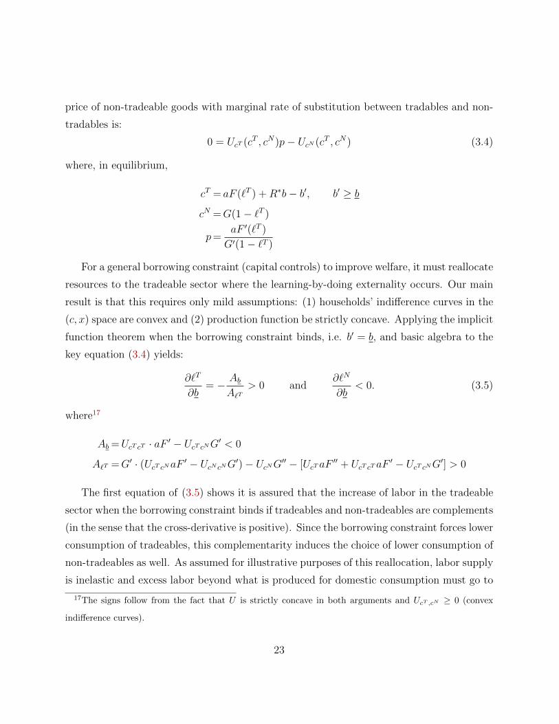
one-sector analysis, with the addition of η = 0.5. We find, as in the one-sector model, the

welfare gain from the optimal borrowing constraint is increasing in the size of the externality,

but is always less than the welfare gain from the Pareto Efficient allocation. The magnitudes

are also similar.

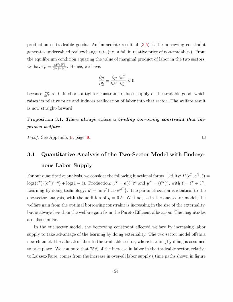
In the one sector model, the borrowing constraint affected welfare by increasing labor

supply to take advantage of the learning by doing externality. The two sector model offers a

new channel. It reallocates labor to the tradeable sector, where learning by doing is assumed

to take place. We compute that 75% of the increase in labor in the tradeable sector, relative

to Laissez-Faire, comes from the increase in over-all labor supply ( time paths shown in figure

24

0.0%

2.0%

4.0%

6.0%

8.0%

0 0.05 0.1 0.15 0.2

Equ

ival

en

t co

nsu

mp

tio

n in

cre

ase

o

ver

LF a

lloca

tio

n

Size of Externality

Optimal Constraints

Pareto Efficient

0.0%

15.0%

30.0%

45.0%

0 0.05 0.1 0.15 0.2

Frac

tio

n o

f P

aret

o E

ffic

ien

t W

elf

are

Gai

ns

Size of Externality

Figure 8: Welfare gains in the 2-sector model

9). For these parameters, the new channel of elastic labor supply we add in this paper is of

a larger magnitude than the classic channel of reallocation studied in previous literature.

-0.12

-0.08

-0.04

0

0.04

0 10 20 30 40 50 60 70 80

Lab

or

w/c

on

str.

le

ss

lab

or

in L

SF

Time

Tradables Total

Figure 9: Change in sectorial labor at optimal constraints versus Laissez-Faire

25

4 The Chinese Experience

In this section, we perform a quantitative analysis of China’s growth experience since opening

trade in 1991. We use our model to infer a sequence of borrowing constraints consistent with

Chinese economic growth and to provide a counterfactual experience under no borrowing

constraints (laissez-faire). This allows us to derive implications for welfare and generate

non-targeted statistics under each scenario. We compare these statistics to the data as

evidence supporting the channels operational in our theory.

We choose to analyze the Chinese economy for three reasons. First, the Chinese economy

is large and has experienced one of the fastest, persistent growth episodes in recent time.

Second, there is evidence aggressive restrictions on borrowing have been placed on households

by the government (or state run banks)18. Third, Chinese growth has been distinguished

by three anomalies that are consistent with our theory: (i) depressed real wage growth, (ii)

undervalued real exchange rate, and (iii) low debt accumulation.

4.1 Quantitative Model

In our quantitative exercise, we consider a 2-sector model with elastic labor 19.

Preferences The period utility function for the household is assumed to take the following

form:

U(cT , cN , `) =G(cT , cN)1−σ

1− σ+ ψ

(1− `)1−ν

1− νwhere

G(cT , cN) =[ωT c

Tη−1η + (1− ωT )cN

η−1η

] ηη−1

Under these preferences, the intertemporal elasticity of consumption and the cross-

elasticity between consumption and leisure, two potentially important margins for our anal-

ysis, can be separately analyzed.

18Interest rate ceilings are well documented. Further, prudential funds mandate savings of 11-30% of

income for some workers, varying by province and time period Sin (2005)19Choice of two sectors allows us to calculate a real exchange rate.

26

The objective is to maximize total life-time utility of all the households given by:∑t

βtU(cT , cN , `t).

Household’s constraints Household’s constraints are standard:

cTt + ptcNt +R∗bt+1≤wt`t + πt +R∗bt (4.1)

bt+1≥ bt (4.2)

The last constraint is the borrowing constraint. For this exercise it is exogenous and not

the result of an optimal policy problem.

Technology Technological and resource constraints are identical to the ones in Section 3.

We consider the following functional forms for production functions and law of motion of

productivity:

yTt =ATt `Tt

α

T tradable good

yNt =ANt `Nt

α

N tradable good

ATt+1 = min{1, ATt · (1 + γ + φ · `Tt )} law of motion (learning by doing)

ANt+1 = min{1, ANt · (1 + γ + φ · `Tt )} law of motion (learning by doing)

where γ is the exogenous productivity catchup and φ is the elasticity of future productivity

with respect to current employment in the tradable sector (the productivity at the world

frontier is normalized to 1). We assume that the learning occurs only in the tradable sector,

but its effect is spilled over to the non-tradable sector20. Such spillover across sectors increases

the potential welfare gains from the borrowing constraints.

20The extent and nature of learning by doing is contentious. Still, several empirical studies support learning

in the traded sector, specifically manufacturing (recently,De Loecker (2007)). The mode of transmission to

the non-tradeable sector can come through development of intermediate goods technology used in each sector

or human capital embodied in workers (Dasgupta (2012)).

27

4.2 Parameters

The model is yearly and we choose a discount factor of β = 0.96. Preference parameters

are ν = 1.69 and σ = 1.5. These provide an inter-temporal elasticity of substitution of

consumption 1/σ = 0.67 which is standard in macroeconomic models. The inter-temporal

elasticity of leisure 1/ν = 0.59, may be larger than often used as motivated by Domeij and

Floden (2006) finding for larger elasticities when controlling for borrowing constraints as are

present in our model.21

The elasticity of substitution is chosen such that traded and non-traded goods are com-

plements (η = 0.05). This elasticity of substitution is most important for the welfare magni-

tudes. We only find welfare gains at reasonable learning by doing parameters for elasticity

of substitution less than 1/10. Therefore, we choose a value within that range.

Table 1: Imposed parameter values

Discount factor β 0.96

elast. of subst. η 0.05

Inter-temp. elast. of subst. 1/σ 0.67

Inter-temp elast. of leisure 1/ν 0.59

Labor shares αT 0.6

αN 0.4

Table 2 presents parameters that have been calibrated. Labor shares in tradeables and

non-tradeables are set to αT = 0.6, and αN = 0.4, respectively, following the multi-country

analysis of Echevarria (1997). The consumption share parameter ωT was calibrated using

the US data. We assumed the United States is the world frontier (AT = AN = 1) and has a

steady-state net foreign asset position of 0. Then, ωT is calibrated so that in the steady-state,

the share of tradable output in GDP equals the average share of manufacturing output in

GDP in the United States in years 1980 - 1991, which is 0.17. This yields ωT = 0.01. While

this parameter seems small, it implies an unextraordinary non-tradeable share of GDP of

70% in the model.

21Varying these elasticities within reasonable ranges has little impact on the welfare results.

28

Table 2: Calibrated parameter values

Parameter Value

Consumption shares ωT 0.01

ωN 1− ωTInitial TFP AT0 0.09

AN0 0.08

Having calibrated ωT , using the US data, we jointly calibrate AT0 and AN0 using the

Chinese data. We match two moments: (i) the ratio of Chinese to American GDP per

capita (assuming AT0 = AN0 = 1 in the United States) and (ii) the share of tradable output

in Chinese GDP in 1991, which equals 0.31. The calibrated values

For our quantitative analysis, we must choose a value for the elasticity of “learning-by-

doing” and a sequence of borrowing constraints. Both are extremely difficult to quantify

directly from empirical observations. Instead, we consider different values for the learning-

by-doing elasticity φ ranging between 0 and 0.08. For a given φ we jointly calibrate the

exogenous growth parameter γ, and the sequence of constraints (bt): the exogenous growth

parameter is calibrated to match the difference between average growth of Chinese and US

real GDP per capita (0.0752) between 1991 and 2007; the sequence of constraints (bt) is

calibrated period-by-period, to match the share of manufacturing output in GDP in China.

4.3 Results

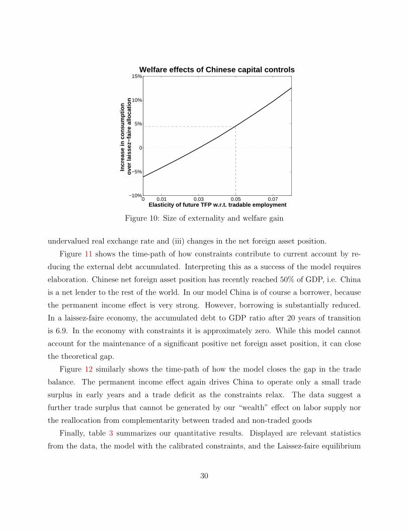
We first show that, at our chosen parameters, Chinese policy can be welfare improving at

moderate LBD elasticities. The result is illustrated in Figure 10. Welfare gains become

positive at an elasticity of 3%. We will choose an elasticity of 5% for the rest of our analysis,

within the typical estimates found in the literature22.

Next, we use our model to measure the contribution of optimal borrowing constraints

to three unique (un-targeted) aspects of the Chinese growth experience: (i) low wages, (ii)

22Fernandes and Isgut (2005) suggest an estimate of 5%. Badinger and Egger (2008) suggest provide

estimates that range between 3% and 8%.

29

0 0.01 0.03 0.05 0.07−10%

−5%

0

5%

10%

15%Welfare effects of Chinese capital controls

Elasticity of future TFP w.r.t. tradable employment

Incr

ease

in c

onsu

mpt

ion

over

lais

sez−

faire

allo

catio

n

Figure 10: Size of externality and welfare gain

undervalued real exchange rate and (iii) changes in the net foreign asset position.

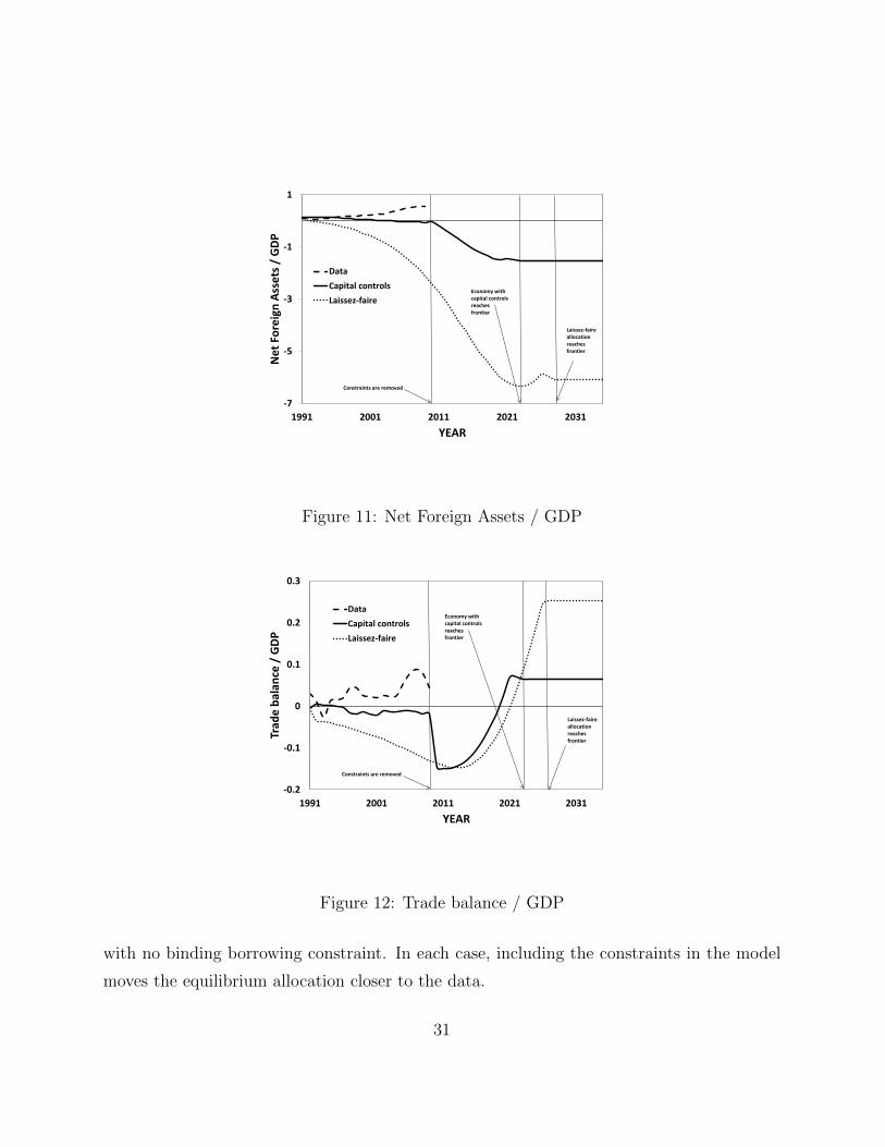
Figure 11 shows the time-path of how constraints contribute to current account by re-

ducing the external debt accumulated. Interpreting this as a success of the model requires

elaboration. Chinese net foreign asset position has recently reached 50% of GDP, i.e. China

is a net lender to the rest of the world. In our model China is of course a borrower, because

the permanent income effect is very strong. However, borrowing is substantially reduced.

In a laissez-faire economy, the accumulated debt to GDP ratio after 20 years of transition

is 6.9. In the economy with constraints it is approximately zero. While this model cannot

account for the maintenance of a significant positive net foreign asset position, it can close

the theoretical gap.

Figure 12 similarly shows the time-path of how the model closes the gap in the trade

balance. The permanent income effect again drives China to operate only a small trade

surplus in early years and a trade deficit as the constraints relax. The data suggest a

further trade surplus that cannot be generated by our “wealth” effect on labor supply nor

the reallocation from complementarity between traded and non-traded goods

Finally, table 3 summarizes our quantitative results. Displayed are relevant statistics

from the data, the model with the calibrated constraints, and the Laissez-faire equilibrium

30

-7

-5

-3

-1

1

1991 2001 2011 2021 2031

Net

For

eign

Ass

ets /

GDP

YEAR

DataCapital controlsLaissez-faire

Laissez-faire allocation reaches frontier

Economy with capital controls reaches frontier

Constraints are removed

Figure 11: Net Foreign Assets / GDP

-0.2

-0.1

0

0.1

0.2

0.3

1991 2001 2011 2021 2031

Trad

e ba

lanc

e /

GDP

YEAR

DataCapital controlsLaissez-faire

Constraints are removed

Laissez-faire allocation reaches frontier

Economy with capital controls reaches frontier

Figure 12: Trade balance / GDP

with no binding borrowing constraint. In each case, including the constraints in the model

moves the equilibrium allocation closer to the data.

31

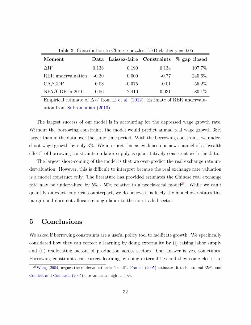
Table 3: Contribution to Chinese puzzles; LBD elasticity = 0.05

Moment Data Laissez-faire Constraints % gap closed

∆W 0.138 0.190 0.134 107.7%

RER undervaluation -0.30 0.000 -0.77 240.6%

CA/GDP 0.03 -0.075 -0.01 55.2%

NFA/GDP in 2010 0.56 -2.410 -0.031 80.1%

Empirical estimate of ∆W from Li et al. (2012). Estimate of RER undervalu-

ation from Subramanian (2010).

The largest success of our model is in accounting for the depressed wage growth rate.

Without the borrowing constraint, the model would predict annual real wage growth 38%

larger than in the data over the same time period. With the borrowing constraint, we under-

shoot wage growth by only 3%. We interpret this as evidence our new channel of a “wealth

effect” of borrowing constraints on labor supply is quantitatively consistent with the data.

The largest short-coming of the model is that we over-predict the real exchange rate un-

dervaluation. However, this is difficult to interpret because the real exchange rate valuation

is a model construct only. The literature has provided estimates the Chinese real exchange

rate may be undervalued by 5% - 50% relative to a neoclassical model23. While we can’t

quantify an exact empirical counterpart, we do believe it is likely the model over-states this

margin and does not allocate enough labor to the non-traded sector.

5 Conclusions

We asked if borrowing constraints are a useful policy tool to facilitate growth. We specifically

considered how they can correct a learning by doing externality by (i) raising labor supply

and (ii) reallocating factors of production across sectors. Our answer is yes, sometimes.

Borrowing constraints can correct learning-by-doing externalities and they come closest to

23Wang (2004) argues the undervaluation is “small”. Frankel (2005) estimates it to be around 35%, and

Coudert and Couharde (2005) cite values as high as 49%.

32

achieving the first best when the externality is not too large or too small.

Our analysis is useful in two ways. First, understanding alternative policy tools has prac-

tical value for policy makers when the availability of standard fiscal and monetary tools is

limited. Second, we have laid theoretical foundations to guide efforts to reconcile contradic-

tory empirical outcomes. We found borrowing constraints distort economies in two ways: by

raising labor supply and reallocating resources across sectors. Further empirical exploration

of these channels could help determine the conditions required for financial repression to

facilitate or hinder growth.

Acknowledgments

For helpful comments we thank Eric Leeper, Jose Victor Rios-Rull and seminar participants

at IU, UT Austin, Purdue, Dallas FED, Federal Reserve Board, Bank of Poland, Midwest

Macroeconomic Meetings at Notre Dame, and Midwest Theory Meetings at Washington

University in St. Louis. All remaining errors are ours.

References

Aizenman, J. and J. Lee (2010): “Real Exchange Rate, Mercantilism And The Learning

By Doing Externality,” Pacific Economic Review, 15, 324–335.

Arrow, K. J. (1962): “The Economic Implications of Learning by Doing,” The Review of

Economic Studies, 29, pp. 155–173.

Badinger, H. and P. Egger (2008): “Intra- and Inter-Industry Productivity Spillovers

in OECD Manufacturing: A Spatial Econometric Perspective,” CESifo Working Paper

Series 2181, CESifo Group Munich.

Benigno, G., H. Chen, C. Otrok, A. Rebucci, and E. R. Young (2013): “Financial

crises and macro-prudential policies,” Journal of International Economics, 89, 453–470.

33

Bianchi, J. (2011): “Overborrowing and Systemic Externalities in the Business Cycle,”

American Economic Review, 101, 3400–3426.

Buera, F. J. and Y. Shin (2009): “Productivity Growth and Capital Flows: The Dynam-

ics of Reforms,” NBER Working Papers 15268, National Bureau of Economic Research,

Inc.

Carroll, C. D. and O. Jeanne (2009): “A Tractable Model of Precautionary Reserves,

Net Foreign Assets, or Sovereign Wealth Funds,” NBER Working Papers 15228, National

Bureau of Economic Research, Inc.

Castaneda, A., J. Diaz-Gimenez, and J.-V. Rios-Rull (2003): “Accounting for the

U.S. Earnings and Wealth Inequality,” Journal of Political Economy, 111, 818–857.

Castro, R., G. L. Clementi, and G. MacDonald (2004): “Investor Protection, Opti-

mal Incentives, and Economic Growth,” The Quarterly Journal of Economics, 119, 1131–

1175.

Costinot, A., G. Lorenzoni, and I. Werning (2011): “A Theory of Capital Controls as

Dynamic Terms-of-Trade Manipulation,” NBER Working Papers 17680, National Bureau

of Economic Research, Inc.

Coudert, V. and C. Couharde (2005): “Real Equilibrium Exchange Rate in China,”

Working Papers 2005-01, CEPII research center.

Dasgupta, K. (2012): “Learning and knowledge diffusion in a global economy,” Journal of

International Economics, 87, 323–336.

De Loecker, J. (2007): “Do exports generate higher productivity? Evidence from Slove-

nia,” Journal of International Economics, 73, 69–98.

Deaton, A. and G. Laroque (1999): “Housing, land prices, and the link between growth

and saving,” Working Papers 223, Princeton University, Woodrow Wilson School of Public

and International Affairs, Research Program in Development Studies.

34

Domeij, D. and M. Floden (2006): “The Labor-Supply Elasticity and Borrowing Con-

straints: Why Estimates are Biased,” Review of Economic Dynamics, 9, 242–262.

Dovis, A. (2012): “Capital Mobility and Optimal Fiscal Policy without Commitment: A

Rationale for Capital Controls?” Mimeo, University of Minnesota.

Du, J., Y. Lu, Z. Tao, and L. Yu (2012): “Do domestic and foreign exporters differ in

learning by exporting? Evidence from China,” China Economic Review, 23, 296–315.

Echevarria, C. (1997): “Changes in Sectoral Composition Associated with Economic

Growth,” International Economic Review, 38, 431–52.

Farhi, E. and I. Werning (2012): “Dealing with the Trilemma: Optimal Capital Controls

with Fixed Exchange Rates,” NBER Working Papers 18199, National Bureau of Economic

Research, Inc.

Fernandes, A. M. and A. E. Isgut (2005): “Learning-by-doing, learning-by-exporting,

and productivity : evidence from Colombia,” Policy Research Working Paper Series 3544,

The World Bank.

Frankel, J. (2005): “On the Renminbi: The Choice between Adjustment under a Fixed

Exchange Rate and Adjustment under a Flexible Rate,” Working Paper 11274, National

Bureau of Economic Research.

Giles, J. and C. Williams (2001a): “Export-led growth: a survey of the empirical litera-

ture and some non-causality results. Part 1,” Journal of International Trade & Economic

Development, 9, 261–337.

——— (2001b): “Export-led growth: a survey of the empirical literature and some non-

causality results. Part 2,” Journal of International Trade & Economic Development, 9,

445–470.

Gourinchas, P.-O. and O. Jeanne (2013): “Capital Flows to Developing Countries:

The Allocation Puzzle,” Review of Economic Studies, Forthcoming.

35

Harrison, A. and A. Rodriguez-Clare (2009): “Trade, Foreign Investment, and In-

dustrial Policy for Developing Countries,” NBER Working Papers 15261, National Bureau

of Economic Research, Inc.

Jappelli, T. and M. Pagano (1994): “Saving, Growth, and Liquidity Constraints,” The

Quarterly Journal of Economics, 109, 83–109.

Jarreau, J. and S. Poncet (2009): “Export Sophistication and Economic Performance:

Evidence from Chinese Provinces,” Working Papers 2009-34, CEPII research center.

Jeske, K. (2006): “Private International Debt with Risk of Repudiation,” Journal of Po-

litical Economy, 114, 576–593.

Korinek, A. (2011): “The New Economics of Capital Controls Imposed for Prudential

Reasons,” IMF Working Papers 11/298, International Monetary Fund.

Korinek, A. and L. Serven (2010): “Undervaluation through foreign reserve accumu-

lation : static losses, dynamic gains,” Policy Research Working Paper Series 5250, The

World Bank.

Li, H., L. Li, B. Wu, and Y. Xiong (2012): “The End of Cheap Chinese Labor,” Journal

of Economic Perspectives, 26, 57–74.

Loecker, J. D. (2010): “A Note on Detecting Learning by Exporting,” NBER Working

Papers 16548, National Bureau of Economic Research, Inc.

Ma, Y. and Y. Zhang (2008): “Whats Different about New Exporters? Evidence from

Chinese Manufacturing Firms,” Tech. rep., Lingnan University.

Mendoza, E. G., V. Quadrini, and J.-V. Ros-Rull (2009): “Financial Integration,

Financial Development, and Global Imbalances,” Journal of Political Economy, 117, 371–

416.

Ostry, J. D., M. S. Qureshi, K. F. Habermeier, D. B. S. Reinhardt, M. Chamon,

and A. R. Ghosh (2010): “Capital Inflows: The Role of Controls,” IMF Staff Position

Notes 2010/04, International Monetary Fund.

36

Pagano, M. (1993): “Financial markets and growth: An overview,” European Economic

Review, 37, 613–622.

Pijoan-Mas, J. (2006): “Precautionary Savings or Working Longer Hours?” Review of

Economic Dynamics, 9, 326–352.

Rodrik, D. (2008): “The Real Exchange Rate and Economic Growth,” Brookings Papers

on Economic Activity, 2008, pp. 365–412.

Romer, P. M. (1986): “Increasing Returns and Long-run Growth,” Journal of Political

Economy, 94, 1002–37.

Schmitt-Grohe, S. and M. Uribe (2012): “Prudential Policy For Peggers,” Tech. rep.,

National Bureau of Economic Research.

Sin, Y. (2005): “Pension liabilities and reform options for old age insurance,” World Bank

working paper.

Song, Z., K. Storesletten, and F. Zilibotti (2011): “Growing Like China,” American

Economic Review, 101, 196–233.

Subramanian, A. (2010): “New PPP-Based Estimates of Renminbi Undervaluation and

Policy Implications,” Policy Briefs PB10-8, Peterson Institute for International Economics.

Wang, T. (2004): “Exchange Rate Dynamics,” in China’s Growth and Integration into the

World Economy, ed. by E. Prasad, International Monetary Fund, vol. 232 of Occasional

Paper, 21 – 28.

Wright, M. L. (2006): “Private capital flows, capital controls, and default risk,” Journal

of International Economics, 69, 120–149.

37

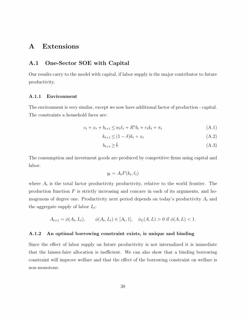
A Extensions

A.1 One-Sector SOE with Capital

Our results carry to the model with capital, if labor supply is the major contributor to future

productivity.

A.1.1 Environment

The environment is very similar, except we now have additional factor of production - capital.

The constraints a household faces are:

ct + xt + bt+1≤wt`t +R∗bt + rtkt + πt (A.1)

kt+1≤ (1− δ)kt + xt (A.2)

bt+1≥ b (A.3)

The consumption and investment goods are produced by competitive firms using capital and

labor:

yt = AtF (kt, `t)

where At is the total factor productivity productivity, relative to the world frontier. The

production function F is strictly increasing and concave in each of its arguments, and ho-

mogenous of degree one. Productivity next period depends on today’s productivity At and

the aggregate supply of labor Lt:

At+1 = φ(At, Lt), φ(At, Lt) ∈ [At, 1], φL(A,L) > 0 if φ(A,L) < 1.

A.1.2 An optimal borrowing constraint exists, is unique and binding

Since the effect of labor supply on future productivity is not internalized it is immediate

that the laissez-faire allocation is inefficient. We can also show that a binding borrowing

constraint will improve welfare and that the effect of the borrowing constraint on welfare is

non-monotone.

38

First, we consider an infinitesimal increase in b above the laissez-faire choice of assets in

one period (with constraints in all future periods not binding): b = B′ + ε. It is enough to

show that such increase will result in higher labor supply today. Suppose not, i.e. L(b) ≤LLF . We will show this must imply lower consumption. The intra-temporal Euler condition

will then imply L(b) > LLF which will be a contradiction.

If L(b) ≤ LLF , then A′(b) ≤ A′LF . Suppose that C(b) ≥ CLF . Then K ′(b) < K ′LF .

Household’s first order condition w.r.t. next period asset holdings imply that UC(C(b),LCE)

βUC(C′LF ,L′LF )

>

R∗, hence 1− δ + A′FK(K ′, L′LF ) > R∗. Notice that if C(b) ≥ CLF , the resource constraint

then implies K ′LF −K ′(b) > b(S)− B′LF , i.e. decrease in the next period’s capital stock is

greater than the increase in net foreign asset position (both relative to laissez-faire policy).

Given that 1−δ+A′FK(K ′, L′LF ) > R∗ - gross return on K ′ is greater than on B′, and given

that A′(b) ≤ A′LF , household’s permanent income falls. That, combined with the decline in

current disposable income (due to forced higher choice of B′) results in C(b) < CLF . In a

competitive equilibrium the following condition must hold:

UC(C(b), L(b))AFL(K,L(b)) + UL(C(b), L(b)) = 0

Since C(b) < CLF we have UC(C,LLF ) > UC(CLF , LLF ) then for the above condition to be

satisfied we must have L > LLF (S), which contradicts our starting assumption. Since we

have shown that L(b) > LLF , the result that A′(b)A

> A′LF

Ais obvious.

Uniqueness again follows from the fact the constraint has non-monotone effect on welfare

(increasing b too much will drive down consumption to zero).

B Proofs

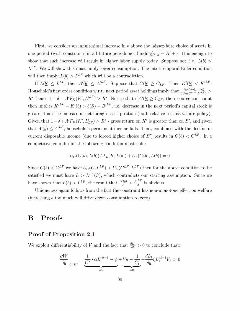
Proof of Proposition 2.1

We exploit differentiability of V and the fact that dL1

db> 0 to conclude that:

∂W

∂b

∣∣∣∣b=B∗

=1

C∗1· αL∗1

α−1 − ψ︸ ︷︷ ︸=0

+VB −1

C∗1︸ ︷︷ ︸=0

+dL1

dbξL∗1

ξ−1VA > 0

39

where ∗ denote the laissez-faire allocations. The first two terms are Euler conditions from

household’s optimization problem and the LF allocations satisfy them. Hence, the only

non-zero term is dL1

dbξL∗1

ξ−1VA > 0. Which yields the existence of a binding constraint that

improves welfare. Uniqueness follows from the fact that W is strictly concave in b, because

V is strictly concave in both A and B.

B.1 Proof of Proposition 3.1

First, notice the value of a laissez-faire allocation is given by:

V LF (a0, b0) = max∑t

βtU(cTt , cNt )

subject to:

at+1 = φ(at, `Tt )

cNt =G(`Nt )

cTt + bt+1 = atF (`Tt ) +R∗bt

UcN (cTt , cNt ) =

atF′(`Tt )

G′(`Nt )UcT (cTt , c

Nt )

UcT (cTt , cNt ) = βR∗UcT (cTt+1, c

Nt+1)

bt+1≥ b

a0, b0 given.

where b is the natural debt limit. Envelope theorem implies that Va > 0.

Let (cT∗t , cN∗t , `Tt

∗, `Nt

∗, b∗t+1, a

∗t+1)

∞t=0 be the laissez-faire allocation. Fix t such that a∗t+1 < 1

and let (a, b) = (a∗t , b∗t ). Define a function:

W (b′; a, b) = max`T ,`N

U(aF (`T ) +R∗b− b′, G(`N)) + βV LF (φ(a, `T ), b′)

subject to (3.4). It is enough to show that:

∂W

∂b′

∣∣∣∣(`T ,`T ,b′)=(`Tt

∗,`Nt∗,b∗t+1)

> 0

40

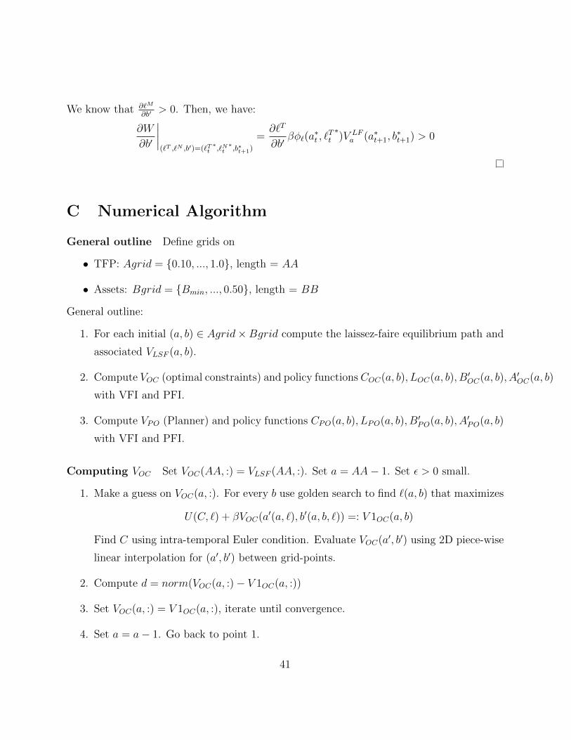
We know that ∂`M

∂b′> 0. Then, we have:

∂W

∂b′

∣∣∣∣(`T ,`N ,b′)=(`Tt

∗,`Nt∗,b∗t+1)

=∂`T

∂b′βφ`(a

∗t , `

Tt

∗)V LF

a (a∗t+1, b∗t+1) > 0

C Numerical Algorithm

General outline Define grids on

• TFP: Agrid = {0.10, ..., 1.0}, length = AA

• Assets: Bgrid = {Bmin, ..., 0.50}, length = BB

General outline:

1. For each initial (a, b) ∈ Agrid×Bgrid compute the laissez-faire equilibrium path and

associated VLSF (a, b).

2. Compute VOC (optimal constraints) and policy functions COC(a, b), LOC(a, b), B′OC(a, b), A′OC(a, b)

with VFI and PFI.

3. Compute VPO (Planner) and policy functions CPO(a, b), LPO(a, b), B′PO(a, b), A′PO(a, b)

with VFI and PFI.

Computing VOC Set VOC(AA, :) = VLSF (AA, :). Set a = AA− 1. Set ε > 0 small.

1. Make a guess on VOC(a, :). For every b use golden search to find `(a, b) that maximizes

U(C, `) + βVOC(a′(a, `), b′(a, b, `)) =: V 1OC(a, b)

Find C using intra-temporal Euler condition. Evaluate VOC(a′, b′) using 2D piece-wise

linear interpolation for (a′, b′) between grid-points.

2. Compute d = norm(VOC(a, :)− V 1OC(a, :))

3. Set VOC(a, :) = V 1OC(a, :), iterate until convergence.

4. Set a = a− 1. Go back to point 1.

41

Computing VPO Set VPO(AA, :) = VLSF (AA, :). Set a = AA− 1. Set ε > 0 small.

1. Make a guess on VPO(a, :) and CPO(a, :). For every b use golden search to find `(a, b)

that maximizes

U(C∗, `) + βVPO(a′(a, `), b′(a, b, `)) =: V 1PO(a, b)

where C∗ must satisfy the inter-temporal Euler condition

C∗−σ = βR∗C ′(a′, b′)−σ

Evaluate V (a′, b′) and C ′(a′, b′) using 2D piece-wise linear interpolation for (a′, b′) be-

tween grid-points. Set C1(a, b) = C∗

2. Compute d1 = norm(VPO(a, :)− V 1PO(a, :)) and d2 = norm(C1(a, :)− CPO(a, :)).

3. If max{d1, d2} < ε, set VPO(a, :) = V 1PO(a, :) and CPO(a, :) = C1(a, :), iterate until

convergence.

4. Set a = a− 1. Go back to point 1.

42