Embed Size (px)
Citation preview
Journal of Graph Algorithms and Applicationshttp://jgaa.info/ vol. 12, no. 1, pp. 73–95 (2008)
Planarity Testing and Optimal Edge Insertion
with Embedding Constraints
Carsten Gutwenger Karsten Klein Petra Mutzel
University of DortmundChair of Algorithm Engineering
Otto-Hahn-Str. 14, 44227 Dortmund, Germany
http://ls11-www.cs.uni-dortmund.de/
[email protected] [email protected]@cs.uni-dortmund.de
Abstract
The planarization method has proven to be successful in graph draw-ing. The output, a combinatorial planar embedding of the so-called pla-narized graph, can be combined with state-of-the-art planar drawing algo-rithms. However, many practical applications have additional constraintson the drawings that result in restrictions on the set of admissible pla-nar embeddings. In this paper, we consider embedding constraints thatrestrict the admissible order of incident edges around a vertex. Such con-straints occur in applications, e.g., from side or port constraints. Weintroduce a set of hierarchical embedding constraints that include group-
ing, oriented, and mirror constraints, and show how these constraints canbe integrated into the planarization method. For this, we first present alinear time algorithm for testing if a given graph G is ec-planar, i.e., ad-mits a planar embedding satisfying the given embedding constraints. Inthe case that G is ec-planar, we provide a linear time algorithm for com-puting the corresponding ec-embedding. Otherwise, an ec-planar subgraphis computed. The critical part is to re-insert the deleted edges subject tothe embedding constraints so that the number of crossings is kept small.For this, we present a linear time algorithm which is able to insert an edgeinto an ec-planar graph H so that the insertion is crossing minimal amongall ec-planar embeddings of H. As a side result, we characterize the setof all possible ec-planar embeddings using BC- and SPQR-trees.
Article Type Communicated by Submitted Revised
Regular paper M. Kaufmann and D. Wagner December 2006 July 2007
C. Gutwenger et al., Embedding Constraints, JGAA, 12(1) 73–95 (2008) 74
1 Introduction
In many application domains information visualization is based on graph repre-sentations. Examples include software engineering, database modeling, businessprocess modeling, VLSI-design, and bioinformatics. The computation of con-cise graph layouts by automatic layout systems facilitates the readability andimmediate understanding of the displayed information. These layout systemsneed to take into account application specific as well as user-defined layout rulesin addition to the aesthetic criteria they try to optimize. In database diagrams,for example, links between attributes should enter the tables only at the left orright side of the corresponding attributes, the placement of reactants in chemi-cal reactions or biological pathways should reflect their role within the displayedreactions, and in UML class diagrams, generalization edges should leave a classobject at the top and enter a base class object at the bottom. Many of theselayout rules impose restrictions on the admissible embeddings for a drawing.Even more important is the possibility to use drawing restrictions in order toexpress the user’s preferences and to guide the layout phase. A general surveyof constraints in graph drawing algorithms is given in [22].
In this paper, we consider restrictions on the allowed order of incident edgesaround a vertex, e.g., to specify groups of edges that have to appear consecu-tively around the vertex or that have a fixed clockwise order in any admissibleembedding. Such constraints occur, e.g., in the form of side constraints, whereincident edges are assigned to the four sides of a rectangular vertex, or portconstraints where edges have prescribed attachment points at a vertex. In par-ticular, we introduce three types of constraints which may be arbitrarily nested:grouping, oriented (prescribed clockwise order), and mirror constraints (pre-scribed reversible order). We call a planar embedding that fulfills the given setof constraints an ec-planar embedding.
An important optimization goal for the computation of graph layouts is theminimization of crossings. The problem of minimizing the number of crossingsin a drawing is NP-hard [14] and no practically efficient method exists so far. Inpractice, the problem is attacked via the planarization approach [1] which firstdeletes a number of edges until the remaining graph is planar and then care-fully reinserts them (iteratively) so that the number of crossings is minimized,see for example [16]. This paper deals with the integration of the embeddingconstraint concept into the planarization approach. The first step can be solvedby successive ec-planarity testing. Our first contribution therefore is a lineartime algorithm for testing if a graph with a set of embedding constraints is ec-planar. The main challenge is to incorporate oriented constraints, where a givenclockwise order of (groups of) incident edges needs to be satisfied. Furthermore,we characterize all possible ec-planar embeddings using BC- and SPQR-trees,which also yields a linear time algorithm for computing an ec-planar embedding.
The second step of the planarization approach can be tackled by repeatedlysolving the optimal edge insertion problem: This problem asks for inserting anedge e = (v, w) into a planar graph so that all crossings involve e and theirnumber is minimized. Alternatively, the problem can be stated as finding an
C. Gutwenger et al., Embedding Constraints, JGAA, 12(1) 73–95 (2008) 75
embedding of a planar graph G where the given edge can be inserted withthe minimum number of crossings. Recently, the problem has been solved inlinear time using the SPQR-tree data structure [17]. The algorithm essentiallycomputes a shortest path Ψ between those nodes in the SPQR-tree T of G
whose skeletons contain v and w, respectively. The optimal insertion path isthen constructed by simply concatenating locally optimal insertion paths of thetree nodes on Ψ.
However, if embedding constraints have to be observed, i.e., restrictions onthe order of the edges around the vertices of G are given, locally optimal solu-tions need not lead to globally optimal solutions and the greedy approach cannotbe applied anymore. The best local decision now depends on the decisions forother parts of the edge insertion path. Our second contribution thus is a newlinear time algorithm to solve the optimal ec-edge insertion problem: Given anec-planar graph G with an additional edge e and a set of embedding constraintsC for the graph G + e, our algorithm computes an ec-planar embedding of G
together with a crossing minimal edge insertion path for e that observes C.Even though constraint handling is an important issue because of its rele-
vance in practical applications, e.g., in interactive graph drawing (see, e.g., [2,21, 6, 5]), there is only few previous work concerning constraints on the admissi-ble embeddings of a graph. Di Battista et al. [9] consider embedding constraintsthat appear in database schemas, where table attributes are arranged from topto bottom within a rectangular vertex representing a table, and links connect-ing attributes may attach at the left or right hand side of these attributes. Theinteger linear programming approach in [13] considers side constraints in theshape computation phase of orthogonal graph drawing. Dornheim [12] studiesthe problem of computing embeddings satisfying topological constraints thatconsist of a cycle together with two sets of edges that have to be embeddedinside or outside the cycle, respectively. Buchheim et al. [7] describe how toadapt the planarization approach for directed graphs when incoming and out-going edges have to appear consecutively around each vertex. On the otherhand, linear time algorithms for planarity testing and embedding are long sinceknown; see [18, 3, 8, 20, 4].
This paper is organized as follows. After recalling some known results onplanar embeddings in Section 2, Section 3 formally defines the embedding con-straints considered in this paper. The first part of the ec-planarity test consistsof transforming the input graph into an ec-expansion which is described in Sec-tion 4; the characterization of ec-planar embeddings and the ec-planarity testitself is then presented in Section 5. Section 6 covers the linear time algorithmfor solving the ec-edge insertion problem. Finally, we conclude the paper withremarks on open problems.
2 Preliminaries
For basic graph terminology, we refer the reader to [11]. A combinatorial em-bedding of a planar graph G is defined as a clockwise ordering of the incident
C. Gutwenger et al., Embedding Constraints, JGAA, 12(1) 73–95 (2008) 76
edges for each vertex with respect to a crossing-free drawing of G in the plane.A planar embedding is a combinatorial embedding together with a fixed externalface.
A block is a maximal 2-connected subgraph. The relationship between blocksand cut vertices is given by the block-cutvertex tree, or BC-tree for short. A slightgeneralization of the BC-tree is the block-vertex tree B of a connected graph G.It represents the relation between the blocks and the vertices of G and containsa B-node for each block of G and a V-node for each vertex of G; a V-node v anda B-node B are connected by an edge if and only if v ∈ B. The representativeof a vertex v of G in block B is either v itself if v ∈ B, or the first vertex on theunique path from B to v in B.
If G is 2-connected, its SPQR-tree T represents the decomposition of G intoits 3-connected components [23] comprising serial, parallel, and 3-connectedstructures. SPQR-trees [10] are formally defined as follows.
A split pair of G is either a separation pair or a pair of adjacent vertices.A split component of a split pair {u, v} is either an edge (u, v) or a maximalsubgraph C of G such that {u, v} is not a split pair of C. Let {s, t} be a splitpair of G. A maximal split pair {u, v} of G with respect to {s, t} is such that,for any other split pair {u′, v′}, vertices u, v, s, and t are in the same splitcomponent.
Let e = (s, t) be an edge of G, called the reference edge. The SPQR-tree Tof G with respect to e is a rooted ordered tree whose nodes are of four types:S, P, Q, and R. Each node µ of T has an associated biconnected multi-graph,called the skeleton of µ (denoted with skeleton(µ)). The tree T is recursivelydefined as follows:
Trivial Case: If G consists of exactly two parallel edges between s and t, thenT consists of a single Q-node whose skeleton is G itself.
Parallel Case: If the split pair {s, t} has at least three split components G1, . . . ,
Gk, the root of T is a P-node µ, whose skeleton consists of k parallel edgese = e1, . . . , ek between s and t.
Series Case: Otherwise, the split pair {s, t} has exactly two split components,one of them is e, and the other one is denoted with G′. If G′ has cut-vertices c1, . . . , ck−1 (k ≥ 2) that partition G into its blocks G1, . . . , Gk,in this order from s to t, the root of T is an S-node µ, whose skeleton isthe cycle e0, e1, . . . , ek, where e0 = e, c0 = s, ck = t, and ei = (ci−1, ci)(i = 1, . . . , k).
Rigid Case: If none of the above cases applies, let {s1, t1}, . . . , {sk, tk} be themaximal split pairs of G with respect to {s, t} (k ≥ 1), and, for i =1, . . . , k, let Gi be the union of all the split components of {si, ti} but theone containing e. The root of T is an R-node, whose skeleton is obtainedfrom G by replacing each subgraph Gi with the edge ei = (si, ti).
Except for the trivial case, µ has children µ1, . . . , µk, such that µi is the rootof the SPQR-tree of Gi ∪ ei with respect to ei (i = 1, . . . , k). The endpoints of
C. Gutwenger et al., Embedding Constraints, JGAA, 12(1) 73–95 (2008) 77
edge ei are called the poles of node µi. Edge ei is said to be the virtual edgeof node µi in skeleton of µ and of node µ in skeleton of µi. We call node µ thepertinent node of ei in skeleton of µi, and µi the pertinent node of ei in skeletonof µ. The virtual edge of µ in skeleton of µi is called the reference edge of µi.
Let µr be the root of T in the decomposition given above. We add a Q-noderepresenting the reference edge e and make it the parent of µr so that it becomesthe new root.
Let e be an edge in skeleton(µ) and ν the pertinent node of e. Deleting edge(µ, ν) in T splits T into two connected components. Let Tν be the connectedcomponent containing ν. The expansion graph of e (denoted with expansion(e))is the graph induced by the edges that are represented by the Q-nodes in Tν .We further introduce the notation expansion+(e) for the graph expansion(e)+e.
Replacing a skeleton edge e by its expansion graph is called expanding e. Thepertinent graph of a tree node µ results from expanding all edges in skeleton(µ)except for the reference edge of µ and is denoted with pertinent(µ). Hence,if e is a skeleton edge and ν its pertinent node, then expansion+(e) equalspertinent(ν). If v is a vertex in G, a node in T whose skeleton contains v iscalled an allocation node of v.
If G is 2-connected and planar, its SPQR-tree T represents all combinato-rial embeddings of G. In particular, a combinatorial embedding of G uniquelydefines a combinatorial embedding of each skeleton in T , and fixing the combi-natorial embedding of each skeleton uniquely defines a combinatorial embeddingof G.
3 Embedding constraints
Let G = (V,E) be a graph. An embedding constraint specifies the admissibleclockwise order of the edges incident to a vertex in a combinatorial embedding ofG. In this paper, we consider the case where a vertex has at most one embeddingconstraint and either all or none of the edges incident to a vertex are subject toembedding constraints.
An embedding constraint at a vertex v ∈ V is a rooted, ordered tree Tv
such that its leaves are exactly the edges incident to v. The inner nodes of Tv,also called constraint-nodes or c-nodes for short, are of three types: oc-nodes(oriented constraint-nodes), mc-nodes (mirror constraint-nodes), and gc-nodes(grouping constraint-nodes). Since Tv is an ordered tree, it imposes an order onits leaves and thus on the edges incident to v. We consider this order as a cyclicorder and represent all admissible cyclic, clockwise orders of the edges incidentto v by defining how the order of the children of c-nodes in Tv can be changed:
gc-node: The order of children may be arbitrarily permuted.
mc-node: The order of children may be reversed.
oc-node: The order of children is fixed.
C. Gutwenger et al., Embedding Constraints, JGAA, 12(1) 73–95 (2008) 78
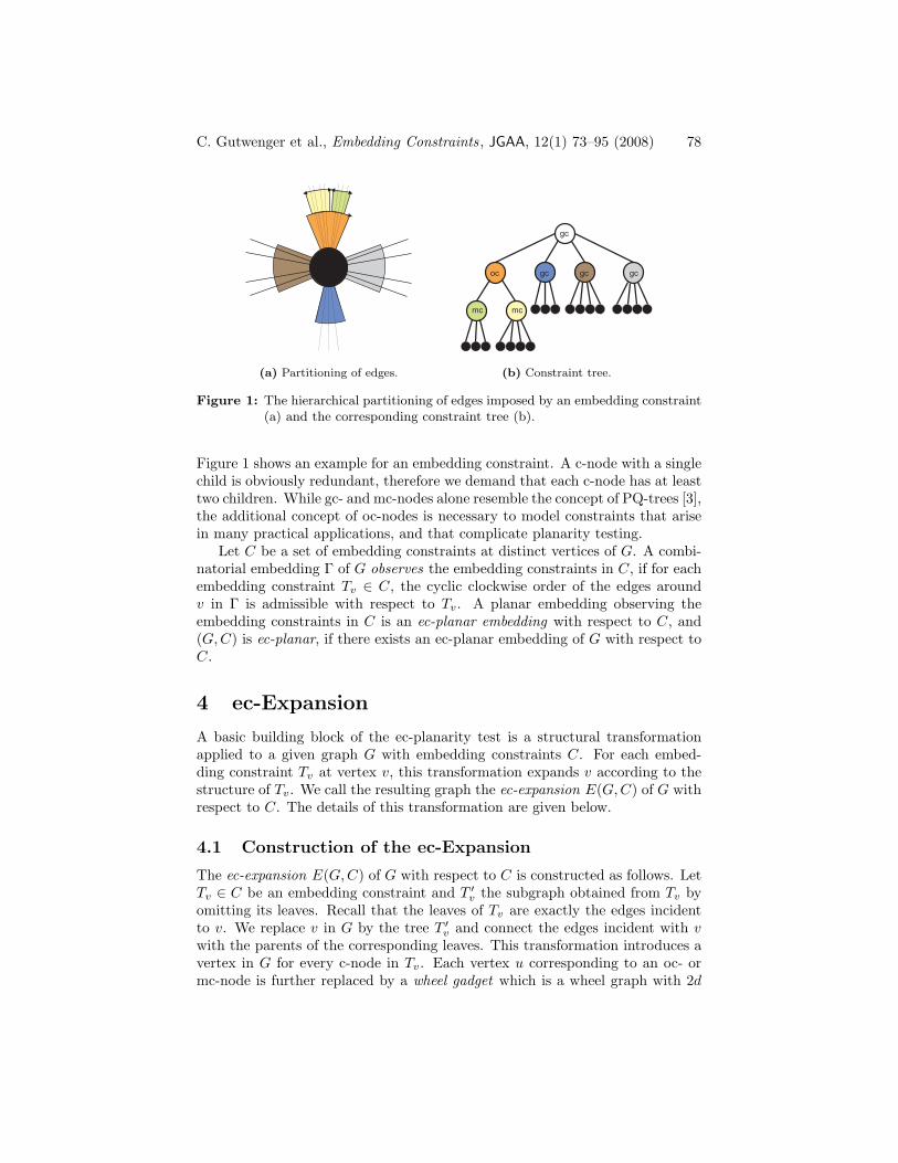
(a) Partitioning of edges.
gc
oc gc gc gc
mc mc
(b) Constraint tree.
Figure 1: The hierarchical partitioning of edges imposed by an embedding constraint(a) and the corresponding constraint tree (b).
Figure 1 shows an example for an embedding constraint. A c-node with a singlechild is obviously redundant, therefore we demand that each c-node has at leasttwo children. While gc- and mc-nodes alone resemble the concept of PQ-trees [3],the additional concept of oc-nodes is necessary to model constraints that arisein many practical applications, and that complicate planarity testing.
Let C be a set of embedding constraints at distinct vertices of G. A combi-natorial embedding Γ of G observes the embedding constraints in C, if for eachembedding constraint Tv ∈ C, the cyclic clockwise order of the edges aroundv in Γ is admissible with respect to Tv. A planar embedding observing theembedding constraints in C is an ec-planar embedding with respect to C, and(G,C) is ec-planar, if there exists an ec-planar embedding of G with respect toC.
4 ec-Expansion
A basic building block of the ec-planarity test is a structural transformationapplied to a given graph G with embedding constraints C. For each embed-ding constraint Tv at vertex v, this transformation expands v according to thestructure of Tv. We call the resulting graph the ec-expansion E(G,C) of G withrespect to C. The details of this transformation are given below.
4.1 Construction of the ec-Expansion
The ec-expansion E(G,C) of G with respect to C is constructed as follows. LetTv ∈ C be an embedding constraint and T ′
v the subgraph obtained from Tv byomitting its leaves. Recall that the leaves of Tv are exactly the edges incidentto v. We replace v in G by the tree T ′
v and connect the edges incident with v
with the parents of the corresponding leaves. This transformation introduces avertex in G for every c-node in Tv. Each vertex u corresponding to an oc- ormc-node is further replaced by a wheel gadget which is a wheel graph with 2d
C. Gutwenger et al., Embedding Constraints, JGAA, 12(1) 73–95 (2008) 79
(a) Wheel gadget. (b) Vertex expansion.
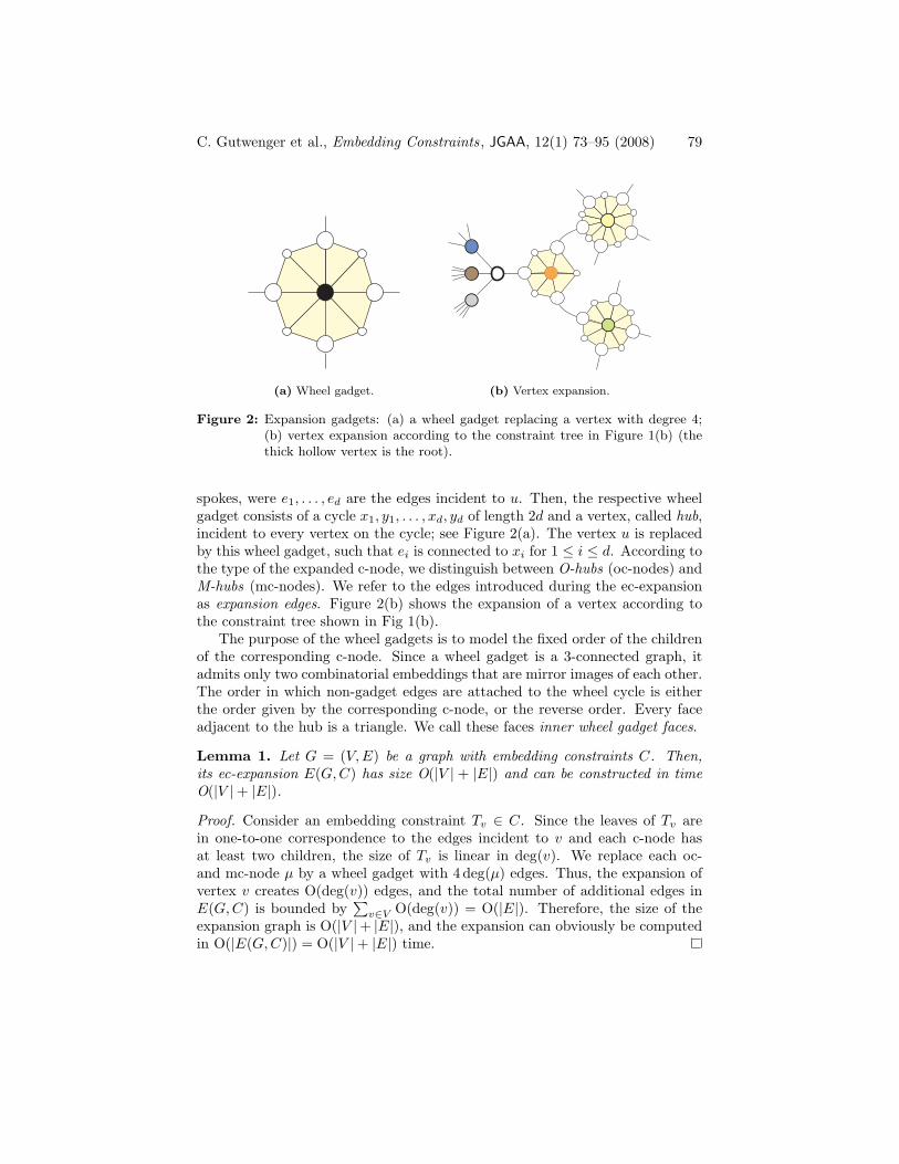
Figure 2: Expansion gadgets: (a) a wheel gadget replacing a vertex with degree 4;(b) vertex expansion according to the constraint tree in Figure 1(b) (thethick hollow vertex is the root).
spokes, were e1, . . . , ed are the edges incident to u. Then, the respective wheelgadget consists of a cycle x1, y1, . . . , xd, yd of length 2d and a vertex, called hub,incident to every vertex on the cycle; see Figure 2(a). The vertex u is replacedby this wheel gadget, such that ei is connected to xi for 1 ≤ i ≤ d. According tothe type of the expanded c-node, we distinguish between O-hubs (oc-nodes) andM-hubs (mc-nodes). We refer to the edges introduced during the ec-expansionas expansion edges. Figure 2(b) shows the expansion of a vertex according tothe constraint tree shown in Fig 1(b).
The purpose of the wheel gadgets is to model the fixed order of the childrenof the corresponding c-node. Since a wheel gadget is a 3-connected graph, itadmits only two combinatorial embeddings that are mirror images of each other.The order in which non-gadget edges are attached to the wheel cycle is eitherthe order given by the corresponding c-node, or the reverse order. Every faceadjacent to the hub is a triangle. We call these faces inner wheel gadget faces.
Lemma 1. Let G = (V,E) be a graph with embedding constraints C. Then,its ec-expansion E(G,C) has size O(|V | + |E|) and can be constructed in timeO(|V | + |E|).
Proof. Consider an embedding constraint Tv ∈ C. Since the leaves of Tv arein one-to-one correspondence to the edges incident to v and each c-node hasat least two children, the size of Tv is linear in deg(v). We replace each oc-and mc-node µ by a wheel gadget with 4 deg(µ) edges. Thus, the expansion ofvertex v creates O(deg(v)) edges, and the total number of additional edges inE(G,C) is bounded by
∑v∈V O(deg(v)) = O(|E|). Therefore, the size of the
expansion graph is O(|V |+ |E|), and the expansion can obviously be computedin O(|E(G,C)|) = O(|V | + |E|) time.
C. Gutwenger et al., Embedding Constraints, JGAA, 12(1) 73–95 (2008) 80
4.2 ec-Expansion and ec-Planar Embeddings
In this section we discuss the relationship between planar embeddings of theec-expansion E(G,C) and ec-planar embeddings of (G,C). Though the ec-expansion serves as a tool for modeling the embedding constraints in C, a planarembedding of E(G,C) needs to fulfill certain conditions in order to induce anec-planar embedding of G with respect to C. We call a planar embedding Γ ofE(G,C) ec-planar if
1. the external face of Γ does not contain a hub;
2. every face incident to a hub is a triangle consisting solely of edges of thecorresponding wheel gadget; and
3. each O-hub h is oriented correctly, i.e., the cyclic, clockwise order of theedges around h in Γ corresponds to the order specified by the correspond-ing oc-node.
Let Γ be an ec-planar embedding of E(G,C). We obtain an ec-planar em-bedding of (G,C) as follows. For each vertex v with corresponding embeddingconstraint in C, there is a connected subgraph Gv in E(G,C) resulting fromexpanding v. Let Gv ⊂ E(G,C) be the graph induced by the vertices not con-tained in Gv. The conditions above assure that the planar embedding Γv ofGv induced by Γ is such that Gv lies in the external face of Γv. The edgesthat connect Gv to Gv correspond to the edges incident to v in G. Their cyclicclockwise order around Gv is admissible with respect to Tv, since the wheelgadgets fix the order of the edges specified by oc- and mc-nodes, and O-hubsare oriented correctly. We shrink Gv to a single vertex by contracting all edgesin Gv while preserving the embedding, thus resulting in an admissible order ofthe edges around v.
If we have an ec-planar embedding of (G,C), then the edges around eachvertex v are ordered such that the constraints in Tv are fulfilled. It is easy to seethat we can replace each such vertex v by the expansion graph correspondingto Tv in such a way that we obtain an ec-planar embedding of E(G,C). Thus,we get the following result:
Lemma 2. Let G be a graph with embedding constraints C. Then, (G,C) is ec-planar if and only if E(G,C) is ec-planar. Moreover, every ec-planar embeddingof E(G,C) induces an ec-planar embedding of (G,C).
5 ec-Planarity Testing
It is well-known that planarity testing can be reduced to 2-connected graphs,i.e., it is sufficient to test the blocks of a graph independently. However, addingembedding constraints complicates this task. Let G be a graph with embeddingconstraints C. Consider a cut vertex c in G that connects two blocks BC1 andBC2 via the edge sets S1 and S2, respectively; see Figure 3(a). If these edge
C. Gutwenger et al., Embedding Constraints, JGAA, 12(1) 73–95 (2008) 81
BC1 BC2
Cut vertex
(a)
BC1 BC2
(b)
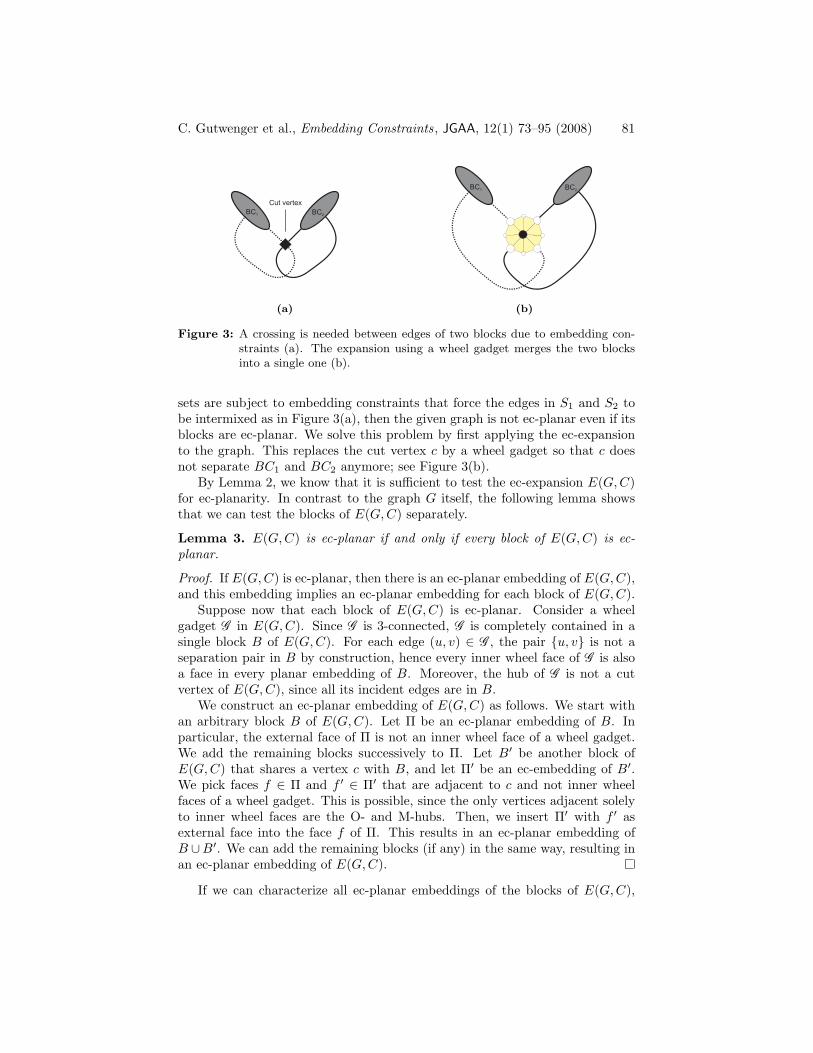
Figure 3: A crossing is needed between edges of two blocks due to embedding con-straints (a). The expansion using a wheel gadget merges the two blocksinto a single one (b).
sets are subject to embedding constraints that force the edges in S1 and S2 tobe intermixed as in Figure 3(a), then the given graph is not ec-planar even if itsblocks are ec-planar. We solve this problem by first applying the ec-expansionto the graph. This replaces the cut vertex c by a wheel gadget so that c doesnot separate BC1 and BC2 anymore; see Figure 3(b).
By Lemma 2, we know that it is sufficient to test the ec-expansion E(G,C)for ec-planarity. In contrast to the graph G itself, the following lemma showsthat we can test the blocks of E(G,C) separately.
Lemma 3. E(G,C) is ec-planar if and only if every block of E(G,C) is ec-planar.
Proof. If E(G,C) is ec-planar, then there is an ec-planar embedding of E(G,C),and this embedding implies an ec-planar embedding for each block of E(G,C).
Suppose now that each block of E(G,C) is ec-planar. Consider a wheelgadget G in E(G,C). Since G is 3-connected, G is completely contained in asingle block B of E(G,C). For each edge (u, v) ∈ G , the pair {u, v} is not aseparation pair in B by construction, hence every inner wheel face of G is alsoa face in every planar embedding of B. Moreover, the hub of G is not a cutvertex of E(G,C), since all its incident edges are in B.
We construct an ec-planar embedding of E(G,C) as follows. We start withan arbitrary block B of E(G,C). Let Π be an ec-planar embedding of B. Inparticular, the external face of Π is not an inner wheel face of a wheel gadget.We add the remaining blocks successively to Π. Let B′ be another block ofE(G,C) that shares a vertex c with B, and let Π′ be an ec-embedding of B′.We pick faces f ∈ Π and f ′ ∈ Π′ that are adjacent to c and not inner wheelfaces of a wheel gadget. This is possible, since the only vertices adjacent solelyto inner wheel faces are the O- and M-hubs. Then, we insert Π′ with f ′ asexternal face into the face f of Π. This results in an ec-planar embedding ofB ∪B′. We can add the remaining blocks (if any) in the same way, resulting inan ec-planar embedding of E(G,C).
If we can characterize all ec-planar embeddings of the blocks of E(G,C),
C. Gutwenger et al., Embedding Constraints, JGAA, 12(1) 73–95 (2008) 82
the construction in the proof of Lemma 3 also shows us how to enumerate allec-planar embeddings of E(G,C) by traversing its BC-tree. In the following,we devise such a characterization. Let B be a block of E(G,C) and T itsSPQR-tree.
Observation 1. Every wheel gadget G is completely contained within the skele-ton of an R-node. In particular, the hub of G occurs only in the skeleton of asingle R-node.
Proof. G is 3-connected, and for each edge (u, v) ∈ G , the pair {u, v} is nota separation pair in B by construction. Therefore, all edges of G occur in thesame skeleton graph, which must be the skeleton of an R-node µ. The hub h ofG is only incident to edges of G and no other edge of B, hence h occurs only inskeleton(µ).
If B is planar, then the skeleton of an R-node is a 3-connected planar graph,thus having exactly two planar embeddings which are mirror images of eachother. We call two O-hubs contained in the same skeleton S conflicting if noneof the two planar embeddings of S orients both O-hubs correctly. The followingtheorem gives us an easy to check condition for ec-planarity and characterizesall possible ec-planar embeddings:
Theorem 1. Let G be a graph with embedding constraints C. Let B be a blockof E(G,C) and T its SPQR-tree. Then, the following holds:
1. B is ec-planar if and only if B is planar and no skeleton of an R-node ofT contains conflicting O-hubs.
2. If B is ec-planar, then the embeddings of the skeletons of T induce anec-planar embedding of B if and only if each O-hub in the skeleton of anR-node is oriented correctly.
Proof. If B admits an ec-planar embedding, then this embedding induces em-beddings of the skeletons of T such that every O-hub in the skeleton of anR-node is oriented correctly. In particular, no R-node skeleton contains con-flicting O-hubs.
Suppose now that B is planar and no R-node skeleton contains conflictingO-hubs. For each R-node skeleton containing at least one O-hub, we can choseplanar embeddings such that all O-hubs are oriented correctly within the skele-tons. We have to show that the embeddings of the skeletons induce an ec-planarembedding of B, even if we chose arbitrary embeddings for the remaining skele-tons. This holds, since every such embedding Π has the property that eachO-hub is oriented correctly because wheel gadgets are completely containedwithin R-node skeletons by Observation 1, and inner wheel faces are preserved.We can pick any face of Π as external face which is not an inner wheel face(such a face always exists) and obtain an ec-planar embedding of B.
Function IsEcPlanar depicted in Algorithm 1 applies Theorem 1 and de-vises a linear time ec-planarity test, which can easily be extended so that itcomputes an ec-planar embedding as well.
C. Gutwenger et al., Embedding Constraints, JGAA, 12(1) 73–95 (2008) 83
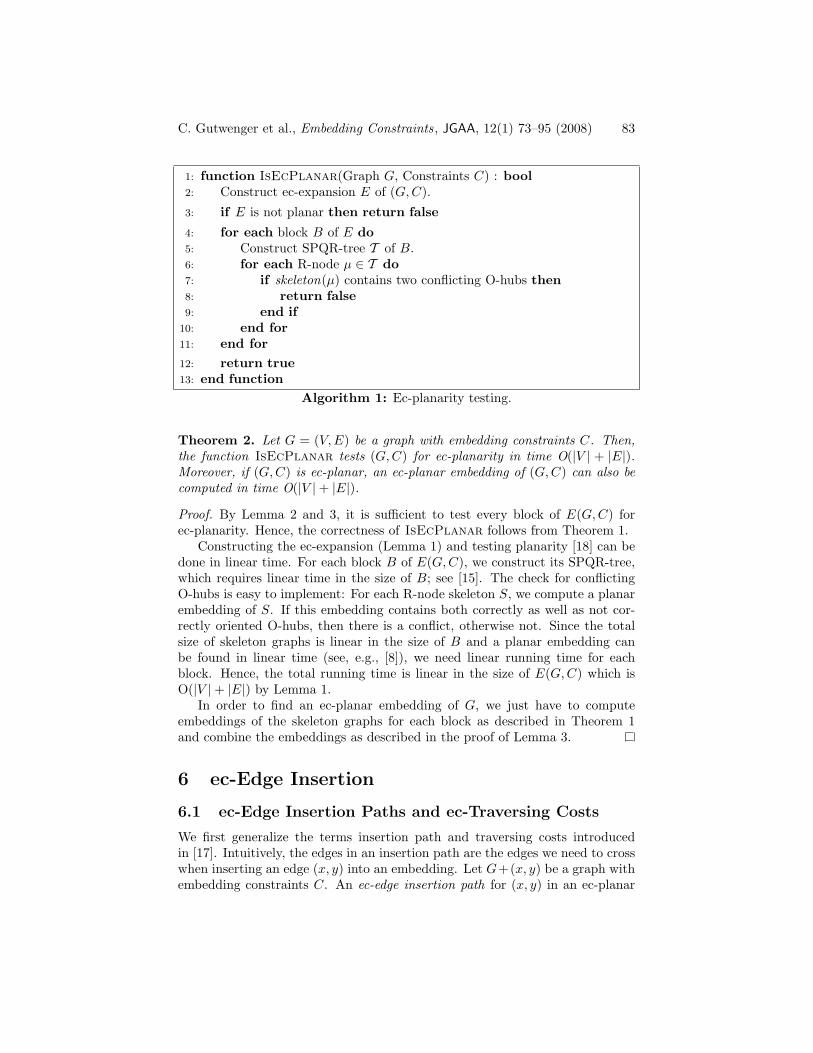
1: function IsEcPlanar(Graph G, Constraints C) : bool
2: Construct ec-expansion E of (G,C).
3: if E is not planar then return false
4: for each block B of E do
5: Construct SPQR-tree T of B.6: for each R-node µ ∈ T do
7: if skeleton(µ) contains two conflicting O-hubs then
8: return false
9: end if
10: end for
11: end for
12: return true
13: end function
Algorithm 1: Ec-planarity testing.
Theorem 2. Let G = (V,E) be a graph with embedding constraints C. Then,the function IsEcPlanar tests (G,C) for ec-planarity in time O(|V | + |E|).Moreover, if (G,C) is ec-planar, an ec-planar embedding of (G,C) can also becomputed in time O(|V | + |E|).
Proof. By Lemma 2 and 3, it is sufficient to test every block of E(G,C) forec-planarity. Hence, the correctness of IsEcPlanar follows from Theorem 1.
Constructing the ec-expansion (Lemma 1) and testing planarity [18] can bedone in linear time. For each block B of E(G,C), we construct its SPQR-tree,which requires linear time in the size of B; see [15]. The check for conflictingO-hubs is easy to implement: For each R-node skeleton S, we compute a planarembedding of S. If this embedding contains both correctly as well as not cor-rectly oriented O-hubs, then there is a conflict, otherwise not. Since the totalsize of skeleton graphs is linear in the size of B and a planar embedding canbe found in linear time (see, e.g., [8]), we need linear running time for eachblock. Hence, the total running time is linear in the size of E(G,C) which isO(|V | + |E|) by Lemma 1.
In order to find an ec-planar embedding of G, we just have to computeembeddings of the skeleton graphs for each block as described in Theorem 1and combine the embeddings as described in the proof of Lemma 3.
6 ec-Edge Insertion
6.1 ec-Edge Insertion Paths and ec-Traversing Costs
We first generalize the terms insertion path and traversing costs introducedin [17]. Intuitively, the edges in an insertion path are the edges we need to crosswhen inserting an edge (x, y) into an embedding. Let G+(x, y) be a graph withembedding constraints C. An ec-edge insertion path for (x, y) in an ec-planar
C. Gutwenger et al., Embedding Constraints, JGAA, 12(1) 73–95 (2008) 84
embedding Π of G is a sequence of edges e1, . . . , ek of G satisfying the followingconditions:
1. There is a face fx ∈ Π with x, e1 ∈ fx, a face fy ∈ Π with ek, y ∈ fy, andfaces fi ∈ Π with ei, ei+1 ∈ fi for 1 ≤ i < k.
2. The edge order around x and y is admissible with respect to C if (x, y)leaves x via face fx and enters y via face fy.
Finding a shortest ec-insertion path in a fixed embedding Π is easy: We onlyneed to identify the set of faces Fx incident to x where the insertion path maystart, and Fy incident to y where it may end, and then find a shortest path inthe dual graph of Π connecting a face in Fx with a face in Fy.
We are interested in the shortest possible ec-insertion path among all ec-planar embeddings of G, which we also call an optimal ec-insertion path in G. Inparticular, we need to identify the required ec-planar embedding of G. In orderto represent all ec-planar embeddings of G, we apply Lemma 2 and use its ec-expansion instead. More precisely, we use the subgraph K = E(G+(x, y), C)\e,where e = (v, w) is the edge of E(G + (x, y), C) connecting the expansion of x
with the expansion of y. An ec-insertion path in an ec-planar embedding of K isdefined as before with the only difference that we replace the second conditionwith
2′. e1, . . . , ek contains no expansion edge of K.
It is easy to see that we can also use this definition for a subgraph B of K andtwo distinct vertices of B that are not hubs.
We adapt the notion of traversing costs defined in [17] to ec-planarity. Lete be a skeleton edge, and let Π be an arbitrary ec-embedding of the graphexpansion+(e) with dual graph Π∗, in which all edges corresponding to gadgetedges have length ∞ and the other edges have length 1. Let f1 and f2 be the twofaces in Π separated by e. We denote with P (Π∗, e) the length of the shortestpath in Π∗ that connects f1 and f2 and does not use the dual edge of e. Hence,we have P (Π∗, e) ∈ N ∪ {∞}.
The following lemma follows analogously to the result shown in [17].
Lemma 4. Let µ be a node in T and e an edge in skeleton(µ). Then, P (Π∗, e)is independent of the ec-embedding Π of expansion+(e).
Proof. Let m be the number of edges in Ge := expansion+(e) and G′
e be thegraph obtained from Ge by replacing each gadget edge with m + 1 paralleledges. Then, each embedding Π of Ge corresponds to an embedding Π′ of G′
e,and P (Π∗, e) is ∞ if and only if the corresponding path in Π′ is longer thanm. Lemma 1 in [17] shows that for the general case, i.e., without embeddingconstraints, P (Π∗, e) is independent of the embedding Π. Applying this lemmaand observing that the ec-embeddings of Ge are a non-empty subset of theembeddings of Ge yields the lemma.
Thus, we define the ec-traversing costs c(e) of a skeleton edge e as P (Π∗, e)for an arbitrary ec-embedding Π of expansion+(e).
C. Gutwenger et al., Embedding Constraints, JGAA, 12(1) 73–95 (2008) 85
6.2 The Algorithm for 2-connected Graphs
The hard part is to find an ec-insertion path in a block B of K. Our task isto compute an optimal ec-insertion path between two nodes v, w of B. Thefunction OptimalEcBlockInserter shown in Algorithm 2 and 3 solves thisproblem. In this algorithms, we use the notation mini,n Λ which returns a tuplein the set Λ of n-tuples whose i-th component is minimal among all tuples in Λ.
The function OptimalEcBlockInserter is called with a block B of anec-planar ec-expansion and two distinct vertices v and w of B. Since we assumethat B contains all gadget edges, we do not need to pass further constraintinformation for the edge (v, w). In particular, using any insertion path in anyec-planar embedding of B that connects v and w and does not cross a gadgetedge yields an ec-embedded planarization of B ∪ (v, w). Hence, we look for anec-embedding of B that allows the insertion of the edge (v, w) with the minimumnumber of crossings.
First, we compute the SPQR-tree T of B and embed the skeletons suchthat they imply an ec-embedding of B, i.e, the R-node skeletons are embeddedcorrectly. Then, the shortest path Υ := µ1, . . . , µk between an allocation nodeµ1 of v and µk of w is identified. In order to achieve a consistent orientation, weroot T such that Υ is a descending path in the tree, i.e., µi is the parent of µi−1
for i = 2, . . . , k. Note that the rooting of the SPQR-tree implies a directionof the skeleton edges: the edges in a skeleton with reference edge er = (s, t)are directed such that the skeleton is a planar st-graph; see, e.g., [10]. Thisdirection is necessary in order to identify the left and the right face of an edge.
The algorithm traverses the path Υ from µ1 to µk−1 and iteratively computesthe lengths of the shortest ec-insertion paths that start from v and leave thepertinent graph Pi of µi to the left or to the right, respectively, where all ec-embeddings of Pi are considered. Here, left and right refer to the direction ofthe reference edge of µi. These lengths are maintained in the variables λℓ andλr. Finally, when node µk is considered, this information is used to determinea shortest insertion path ending at w.
For each node µi, the following information is computed:
• φiℓ (resp. φi
r) indicates if the shortest ec-insertion path leaving Pi to theleft (right) uses the shortest ec-insertion path that leaves Pi−1 to the left(in this case the value is ℓ) or to the right (the value is r).
• ∆iℓ (resp. ∆i
r) is the subpath that is appended to the path leaving Pi−1
when leaving Pi to the left (right).
These values are solely used for the purpose of creating the optimal ec-insertionpath at the end of the function. If s ∈ {ℓ, r} denotes a side, we denote with s
the other side, i.e., ℓ = r and vice versa.The body of the for-loop starts by expanding all edges of the skeleton Si of
µi except for edges representing v or w. The resulting graph is called Gi. If1 < i < k, then Gi will contain two virtual edges ev (representing v) and ew
(representing w). Note that we obtain Pi (plus reference edge) by replacing ev
with Pi−1.
C. Gutwenger et al., Embedding Constraints, JGAA, 12(1) 73–95 (2008) 86
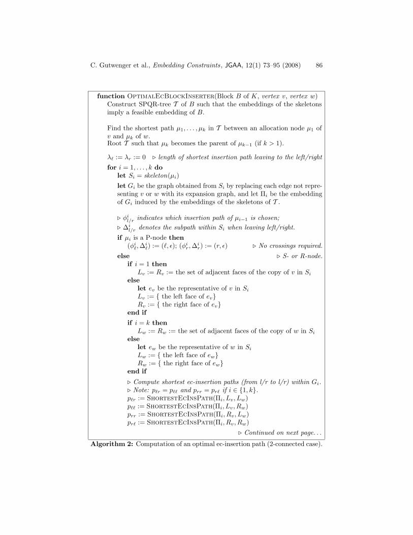
function OptimalEcBlockInserter(Block B of K, vertex v, vertex w)Construct SPQR-tree T of B such that the embeddings of the skeletonsimply a feasible embedding of B.
Find the shortest path µ1, . . . , µk in T between an allocation node µ1 ofv and µk of w.Root T such that µk becomes the parent of µk−1 (if k > 1).
λℓ := λr := 0 ⊲ length of shortest insertion path leaving to the left/right
for i = 1, . . . , k do
let Si = skeleton(µi)
let Gi be the graph obtained from Si by replacing each edge not repre-senting v or w with its expansion graph, and let Πi be the embeddingof Gi induced by the embeddings of the skeletons of T .
⊲ φil/r indicates which insertion path of µi−1 is chosen;
⊲ ∆il/r denotes the subpath within Si when leaving left/right.
if µi is a P-node then
(φiℓ,∆
iℓ) := (ℓ, ǫ); (φi
r,∆ir) := (r, ǫ) ⊲ No crossings required.
else ⊲ S- or R-node.if i = 1 then
Lv := Rv := the set of adjacent faces of the copy of v in Si
else
let ev be the representative of v in Si
Lv := { the left face of ev}Rv := { the right face of ev}
end if
if i = k then
Lw := Rw := the set of adjacent faces of the copy of w in Si
else
let ew be the representative of w in Si
Lw := { the left face of ew}Rw := { the right face of ew}
end if
⊲ Compute shortest ec-insertion paths (from l/r to l/r) within Gi.⊲ Note: pℓr = pℓℓ and prr = prℓ if i ∈ {1, k}.pℓr := ShortestEcInsPath(Πi, Lv, Lw)pℓℓ := ShortestEcInsPath(Πi, Lv, Rw)prr := ShortestEcInsPath(Πi, Rv, Lw)prℓ := ShortestEcInsPath(Πi, Rv, Rw)
⊲ Continued on next page. . .
Algorithm 2: Computation of an optimal ec-insertion path (2-connected case).
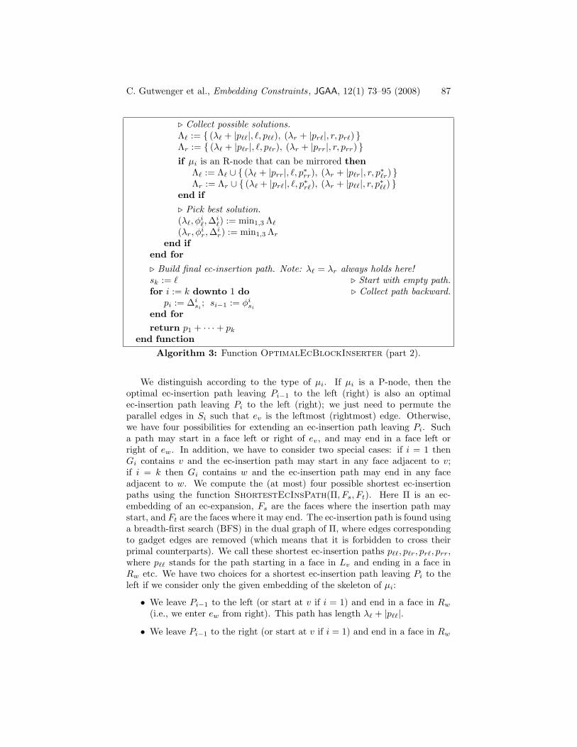
C. Gutwenger et al., Embedding Constraints, JGAA, 12(1) 73–95 (2008) 87
⊲ Collect possible solutions.Λℓ := { (λℓ + |pℓℓ|, ℓ, pℓℓ), (λr + |prℓ|, r, prℓ) }Λr := { (λℓ + |pℓr|, ℓ, pℓr), (λr + |prr|, r, prr) }
if µi is an R-node that can be mirrored then
Λℓ := Λℓ ∪ { (λℓ + |prr|, ℓ, p∗
rr), (λr + |pℓr|, r, p∗
ℓr) }Λr := Λr ∪ { (λℓ + |prℓ|, ℓ, p
∗
rℓ), (λr + |pℓℓ|, r, p∗
ℓℓ) }end if
⊲ Pick best solution.(λℓ, φ
iℓ,∆
iℓ) := min1,3 Λℓ
(λr, φir,∆
ir) := min1,3 Λr
end if
end for
⊲ Build final ec-insertion path. Note: λℓ = λr always holds here!sk := ℓ ⊲ Start with empty path.for i := k downto 1 do ⊲ Collect path backward.
pi := ∆isi
; si−1 := φisi
end for
return p1 + · · · + pk
end function
Algorithm 3: Function OptimalEcBlockInserter (part 2).
We distinguish according to the type of µi. If µi is a P-node, then theoptimal ec-insertion path leaving Pi−1 to the left (right) is also an optimalec-insertion path leaving Pi to the left (right); we just need to permute theparallel edges in Si such that ev is the leftmost (rightmost) edge. Otherwise,we have four possibilities for extending an ec-insertion path leaving Pi. Sucha path may start in a face left or right of ev, and may end in a face left orright of ew. In addition, we have to consider two special cases: if i = 1 thenGi contains v and the ec-insertion path may start in any face adjacent to v;if i = k then Gi contains w and the ec-insertion path may end in any faceadjacent to w. We compute the (at most) four possible shortest ec-insertionpaths using the function ShortestEcInsPath(Π, Fs, Ft). Here Π is an ec-embedding of an ec-expansion, Fs are the faces where the insertion path maystart, and Ft are the faces where it may end. The ec-insertion path is found usinga breadth-first search (BFS) in the dual graph of Π, where edges correspondingto gadget edges are removed (which means that it is forbidden to cross theirprimal counterparts). We call these shortest ec-insertion paths pℓℓ, pℓr, prℓ, prr,where pℓℓ stands for the path starting in a face in Lv and ending in a face inRw etc. We have two choices for a shortest ec-insertion path leaving Pi to theleft if we consider only the given embedding of the skeleton of µi:
• We leave Pi−1 to the left (or start at v if i = 1) and end in a face in Rw
(i.e., we enter ew from right). This path has length λℓ + |pℓℓ|.
• We leave Pi−1 to the right (or start at v if i = 1) and end in a face in Rw
C. Gutwenger et al., Embedding Constraints, JGAA, 12(1) 73–95 (2008) 88
(i.e., we enter ew from left). This path has length λr + |prℓ|.
For the shortest ec-insertion path leaving Pi to the right, we have two similarcases. Further choices are possible if µi is an R-node that can be mirrored. Wecould mirror the embedding of Si, expand the skeleton edges as before such thatwe obtain an embedding Πi, and compute the four paths in Πi again. Noticethat Πi is not simply the mirror image of Πi. However, this is not necessary.We observe that, e.g., the path pℓℓ is obtained from prr by reversing the subse-quences of edges that have been created by expanding a common skeleton edgeof Si. We call this path p∗rr. A similar argumentation holds for pℓr, prℓ, prr. Itfollows that we have at most four possible choices for leaving Pi to the left andto the right, respectively. Among all possible choices, we pick the shortest one.
After processing all nodes µi, it is easy to reconstruct the best ec-insertionpath from v to w using φi
ℓ/r and ∆iℓ/r. Notice that λℓ = λr holds at the end,
since Lkw = Rk
w.
6.3 Correctness and Optimality
Lemma 5. There exists an ec-embedding Π of B such that p1 + · · · + pk is anec-insertion path for v and w in B with respect to Π.
Proof. Consider the path Υ = µ1, . . . , µk computed by the algorithm. By con-struction of Υ, the skeleton of µ1 contains v, the skeleton of µk contains w, and,for each j = 2, . . . , k− 1, the skeleton of µj contains neither v nor w. Moreover,Υ does not contain a Q-node.
First, we prove the lemma for the case where Υ consists of a single node µ1.In this case, the skeleton of µ1 contains both v and w. We distinguish two casesaccording to the type of µ1:
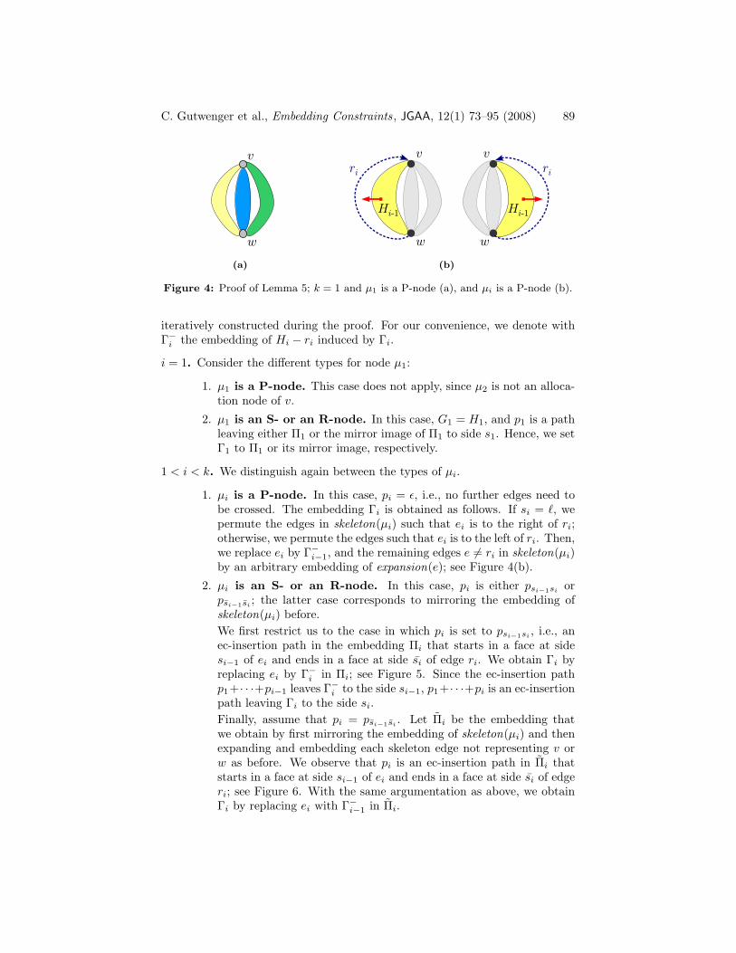
1. µ1 is a P-node. Let Π be an arbitrary ec-embedding of B. Since v andw share a common face in Π, the empty path returned by the algorithm isan ec-insertion path for v and w in B with respect to Π; see Figure 4(a).
2. µ1 is an S- or an R-node. In this case the graph G1 constructed by thealgorithm is the original block B, since all skeleton edges are expanded.Moreover, Π1 is an ec-embedding of B, and pℓr = pℓℓ and prr = prℓ areec-insertion paths in B with respect to Π1. We do not need to considerthe case where the embedding of the skeleton can be mirrored, since thiswill not yield a shorter path. Hence, p1 is either pℓr or prr and thus anec-insertion path in B with respect to Π1.
Assume now that k > 1. For i = 1, . . . , k, we denote with Hi the pertinentgraph of µi, with ri the reference edge of µi in Hi, and, for 1 < i, with ei theedge in skeleton(µi) whose pertinent node is µi−1. Recall that si ∈ {ℓ, r} is theside of Hi where the computed insertion path shall leave. We show by inductionover i that, for 1 ≤ i < k, there is an embedding Γi of Hi such that p1 + · · ·+ pi
is an ec-insertion path leaving Hi at side si. The embeddings Γ1, . . . ,Γk−1 are
C. Gutwenger et al., Embedding Constraints, JGAA, 12(1) 73–95 (2008) 89
(a) (b)
Figure 4: Proof of Lemma 5; k = 1 and µ1 is a P-node (a), and µi is a P-node (b).
iteratively constructed during the proof. For our convenience, we denote withΓ−
i the embedding of Hi − ri induced by Γi.
i = 1. Consider the different types for node µ1:
1. µ1 is a P-node. This case does not apply, since µ2 is not an alloca-tion node of v.
2. µ1 is an S- or an R-node. In this case, G1 = H1, and p1 is a pathleaving either Π1 or the mirror image of Π1 to side s1. Hence, we setΓ1 to Π1 or its mirror image, respectively.
1 < i < k. We distinguish again between the types of µi.
1. µi is a P-node. In this case, pi = ǫ, i.e., no further edges need tobe crossed. The embedding Γi is obtained as follows. If si = ℓ, wepermute the edges in skeleton(µi) such that ei is to the right of ri;otherwise, we permute the edges such that ei is to the left of ri. Then,we replace ei by Γ−
i−1, and the remaining edges e 6= ri in skeleton(µi)
by an arbitrary embedding of expansion(e); see Figure 4(b).
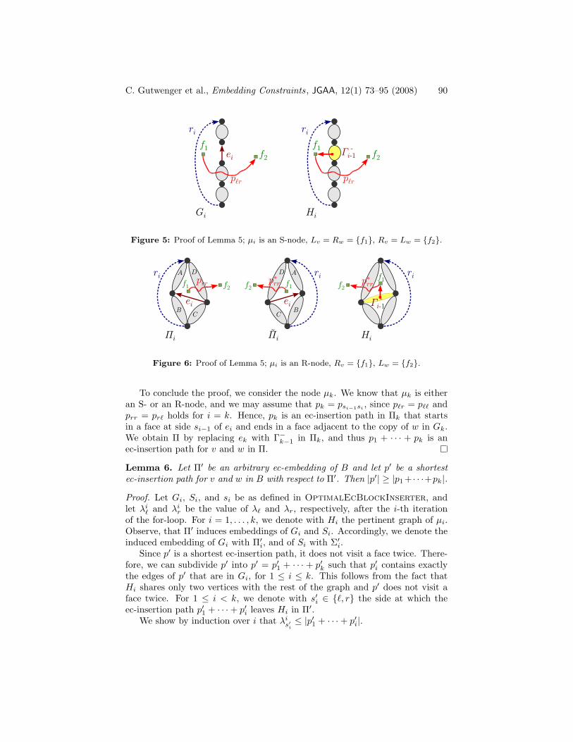
2. µi is an S- or an R-node. In this case, pi is either psi−1sior
psi−1si; the latter case corresponds to mirroring the embedding of
skeleton(µi) before.
We first restrict us to the case in which pi is set to psi−1si, i.e., an
ec-insertion path in the embedding Πi that starts in a face at sidesi−1 of ei and ends in a face at side si of edge ri. We obtain Γi byreplacing ei by Γ−
i in Πi; see Figure 5. Since the ec-insertion pathp1+· · ·+pi−1 leaves Γ−
i to the side si−1, p1+· · ·+pi is an ec-insertionpath leaving Γi to the side si.
Finally, assume that pi = psi−1si. Let Πi be the embedding that
we obtain by first mirroring the embedding of skeleton(µi) and thenexpanding and embedding each skeleton edge not representing v orw as before. We observe that pi is an ec-insertion path in Πi thatstarts in a face at side si−1 of ei and ends in a face at side si of edgeri; see Figure 6. With the same argumentation as above, we obtainΓi by replacing ei with Γ−
i−1in Πi.
C. Gutwenger et al., Embedding Constraints, JGAA, 12(1) 73–95 (2008) 90
Figure 5: Proof of Lemma 5; µi is an S-node, Lv = Rw = {f1}, Rv = Lw = {f2}.
Figure 6: Proof of Lemma 5; µi is an R-node, Rv = {f1}, Lw = {f2}.
To conclude the proof, we consider the node µk. We know that µk is eitheran S- or an R-node, and we may assume that pk = psi−1si
, since pℓr = pℓℓ andprr = prℓ holds for i = k. Hence, pk is an ec-insertion path in Πk that startsin a face at side si−1 of ei and ends in a face adjacent to the copy of w in Gk.We obtain Π by replacing ek with Γ−
k−1in Πk, and thus p1 + · · · + pk is an
ec-insertion path for v and w in Π.
Lemma 6. Let Π′ be an arbitrary ec-embedding of B and let p′ be a shortestec-insertion path for v and w in B with respect to Π′. Then |p′| ≥ |p1 + · · ·+pk|.
Proof. Let Gi, Si, and si be as defined in OptimalEcBlockInserter, andlet λi
ℓ and λir be the value of λℓ and λr, respectively, after the i-th iteration
of the for-loop. For i = 1, . . . , k, we denote with Hi the pertinent graph of µi.Observe, that Π′ induces embeddings of Gi and Si. Accordingly, we denote theinduced embedding of Gi with Π′
i, and of Si with Σ′
i.Since p′ is a shortest ec-insertion path, it does not visit a face twice. There-
fore, we can subdivide p′ into p′ = p′1 + · · · + p′k such that p′i contains exactlythe edges of p′ that are in Gi, for 1 ≤ i ≤ k. This follows from the fact thatHi shares only two vertices with the rest of the graph and p′ does not visit aface twice. For 1 ≤ i < k, we denote with s′i ∈ {ℓ, r} the side at which theec-insertion path p′1 + · · · + p′i leaves Hi in Π′.
We show by induction over i that λis′
i≤ |p′1 + · · · + p′i|.
C. Gutwenger et al., Embedding Constraints, JGAA, 12(1) 73–95 (2008) 91
i = 1. If k = 1, then G1 = B and the proposition follows immediately, soassume k > 1. If µ1 is not an R-node, then λs′
1= 0 and the proposition
follows immediately. Otherwise, the algorithm also computes the shortestec-insertion path leaving at side s′1 in Σ′
1, where the costs of the edges aretheir traversing costs. Since the traversing costs are independent of theembedding by Lemma 4, we get λ1
s′
1
≤ |p′1|.
1 < i < k. Assume now that λjs′
j
≤ |p′1 + · · ·+ p′j | for 1 ≤ j < i. We distinguish
two cases:
1. µi is a P-node. In this case, we have s′i−1 = s′i, since pi + · · · + pk
does not contain an edge of Hi−1. This yields
λis′
i= λi−1
s′
i−1
≤ |p′1 + · · · + p′i−1| ≤ |p′1 + · · · + p′i|.
2. µi is an S- or an R-node. Observe that p′i is an ec-insertion pathin Π′
i starting in the face at side s′i of the edge representing v andending in a face at side s′i+1 of the edge representing w if i < k, ora face adjacent to w otherwise. This implies an ec-insertion path inΣ′
i, where the costs of a skeleton edge are its traversing costs. Onthe other hand, the algorithm computes a shortest ec-insertion pathin Σ′
i, since the traversing costs of a skeleton edge are independentof the embedding by Lemma 4. Thus, we get λs′
i− λs′
i−1≤ |p′i|, and
henceλs′
i≤ λs′
i−1+ |pi| ≤ |p′1 + · · · + p′i|.
Finally, we get |p1 + · · · + pk| = λis′
i≤ |p′| and the lemma holds.
Theorem 3. Let B = (V,E) be a block of K and let v and w be two distinct ver-tices of B. Then, function OptimalEcBlockInserter computes an optimalec-insertion path for v and w in B in time O(|E|).
Proof. The correctness and optimality of the algorithm follows from Lemma 5and Lemma 6. Constructing the SPQR-tree and embedding the skeleton graphstakes time O(|E|); see [15, 19, 8]. Let Gi = (Vi, Ei) be the graph consideredin each iteration of the for-loop. Then, each iteration takes time O(|Ei|), sinceShortestEcInsPath takes only time linear in the size of Gi by applying BFS.Moreover, the set Ei consists of some edges E′
i of G plus at most two virtualedges (the representatives of v and w). Thus, |E1| + · · · + |Ek| = O(|E|), andhence we get a total running time of O(|E|).
6.4 Generalization to Connected Graphs
The edge insertion algorithm can easily be generalized to connected graphs byusing the same technique as in [17] for the unconstrained case; see Alg. 4. Foreach block Bi on the path from v to w in the block-vertex tree B of G, wecompute the optimal ec-edge insertion path pi between the representatives of
C. Gutwenger et al., Embedding Constraints, JGAA, 12(1) 73–95 (2008) 92
function OptimalEcInserter(ec-expansion G, vertex v, vertex w)Compute the block-vertex tree B of G
Find the path v,B1, c1, . . . , Bk−1, ck−1, Bk, w from v to w in B.
for i := 1, . . . , k do
let xi and yi be the representatives of v and w in Bi
pi := OptimalEcBlockInserter(Bi, xi, yi)end for
return p1 + · · · + pk
end function
Algorithm 4: Computation of an optimal ec-insertion path.
v and w with a corresponding ec-planar embedding Πi. Then, we concatenatethese ec-edge insertion paths building the optimal ec-edge insertion path for v
and w.The correctness proof in [17] uses induction over the number of blocks on
the path from v to w in B. We briefly recall this proof. Let B1, . . . , Bk bethe blocks on this path and let Hi be the union of the blocks B1 to Bi. LetΠi be an embedding of Bi such that pi is an optimal edge insertion path forthe representatives xi and yi in Bi with respect to Πi. Let Ψi denote theconcatenation p1 + · · · + pi.
An embedding Γi for Hi with an optimal edge insertion path Ψi can beiteratively constructed by combining the embedding Γi−1 for Hi−1 and the em-bedding Πi for block Bi. Both yi−1 and xi denote the same vertex in G andthere exist optimal edge insertion paths Ψi−1 for v1 and yi−1 as well as pi forxi and yi. Therefore there is a face f ∈ Γi−1 that contains yi−1 and either v1
if Ψi−1 is empty or the last edge in Ψi−1. Similarly, there is a face f ′ ∈ Πi
that contains xi and either yi if pi is empty or the first edge in pi. We candirectly concatenate the two paths if both faces coincide. This can be achievedby choosing f as the external face of Γi−1 and placing this embedding of Hi−1
into face f ′ of Πi. Then Ψi is an optimal ec-insertion path for v1 and yi in Hi
with respect to Γi.We need to show that—under the presence of embedding constraints—ec-
planarity is preserved, i.e., Γk is still an ec-planar embedding. The only criticalaspect in each step is the selection of f as the external face; but this does notchange the clockwise order of the edges around the vertices of G. Furthermore,we ensure in the computation of the ec-edge insertion paths pi that we do notcross any expansion edges. Hence, we know that the paths Ψi−1 and pi do notstart or end in a face containing a hub. Therefore, the ec-planarity conditionsare still fulfilled and Γk is ec-planar.
It is obvious that p1 + · · ·+ pk is an ec-edge insertion path for v and w withrespect to an embedding Π that results from inserting the remaining blocksnot contained in Hk (as shown in the proof of Lemma 3) into Γk. The lengthof the computed ec-edge insertion path is obviously minimal, since a shorterpath would imply that there exists a shorter path within a block. The block-
C. Gutwenger et al., Embedding Constraints, JGAA, 12(1) 73–95 (2008) 93
vertex tree of a graph can be constructed in linear time and the running timeof OptimalEcBlockInserter(Bi, xi, yi) is linear in the size of the block Bi
(Theorem 3), thus yielding linear running time for OptimalEcInserter.Together with Lemma 1, we obtain the following result:
Theorem 4. Let G = (V,E) be a graph with embedding constraints C ande = (v, w) ∈ E such that G − e is ec-planar. Then, we can compute an optimalec-edge insertion path for (v, w) in G − e in O(|V | + |E|) time.
7 Conclusion and Future Work
We introduced a flexible concept of embedding constraints which allows us tomodel a wide range of constraints on the order of edges incident to a vertex.We presented a linear time algorithm for testing ec-planarity, as well as a char-acterization of all possible ec-embeddings. The latter is in particular importantfor developing algorithms that optimize over the set of all ec-planar embed-dings. We showed that optimal edge insertion can still be performed in lineartime when embedding constraints have to be respected. In order to devise prac-tically successful graph drawing algorithms, the following problems should beconsidered:
• Develop faster algorithms for finding ec-planar subgraphs.
• Solve the so-called orientation problem for orthogonal graph drawing, e.g.,allow us to fix some edges to attach only at the top side of a rectangularvertex. The problem arises when angles are assigned at each vertex be-tween adjacent edges to fix the assignment to the vertex’s sides, e.g., innetwork flow based drawing approaches. The vertices then need to be ori-ented such that the edges that are assigned to the same sides at differentvertices are aligned.
• In some applications, only a subset of the edges is subject to embeddingconstraints at a vertex v, i.e., some edges can attach at arbitrary positions.Hence, we wish to extend the concept of embedding constraints for so-called free edges that are not contained in the tree Tv.
C. Gutwenger et al., Embedding Constraints, JGAA, 12(1) 73–95 (2008) 94
References
[1] C. Batini, M. Talamo, and R. Tamassia. Computer aided layout of entityrelationship diagrams. Journal of Systems and Software, 4:163–173, 1984.
[2] K.-F. Bohringer and F. N. Paulisch. Using constraints to achieve stabilityin automatic graph layout algorithms. In Proc. of CHI-90, pages 43–51,Seattle, WA, 1990.
[3] K. S. Booth and G. S. Lueker. Testing for the consecutive ones property,interval graphs, and graph planarity using P-Q tree algorithms. Journal ofComputer and System Sciences, 13:335–379, 1976.
[4] J. Boyer and W. Myrvold. On the cutting edge: Simplified O(n) planarityby edge addition. Journal on Graph Algorithms and Applications, 8(3):241–273, 2004.
[5] U. Brandes, M. Eiglsperger, M. Kaufmann, and D. Wagner. Sketch-drivenorthogonal graph drawing. In Proc. 10th Intl. Symp. Graph Drawing (GD2002), volume 2528 of LNCS, pages 1–11, 2002.
[6] U. Brandes and D. Wagner. A bayesian paradigm for dynamic graph layout.In Graph Drawing, pages 236–247, 1997.
[7] C. Buchheim, M. Junger, A. Menze, and M. Percan. Bimodal crossingminimization. In D. Z. Chen and D. T. Lee, editors, COCOON, volume4112 of LNCS, pages 497–506. Springer, 2006.
[8] N. Chiba, T. Nishizeki, S. Abe, and T. Ozawa. A linear algorithm forembedding planar graphs using PQ-trees. Journal of Computer and SystemSciences, 30:54–76, 1985.
[9] G. Di Battista, W. Didimo, M. Patrignani, and M. Pizzonia. Drawingdatabase schemas. Software: Practice and Experience, 32(11):1065–1098,2002.
[10] G. Di Battista and R. Tamassia. On-line planarity testing. SIAM Journalon Computing, 25(5):956–997, 1996.
[11] R. Diestel. Graph Theory, volume 173 of Graduate Texts in Mathematics.Springer, third edition, 2005.
[12] C. Dornheim. Planar graphs with topological constraints. Journal on GraphAlgorithms and Applications, 6(1):27–66, 2002.
[13] M. Eiglsperger, U. Foßmeier, and M. Kaufmann. Orthogonal graph drawingwith constraints. In Proc. of the 11th ACM-SIAM Symp. on Discr. Alg.,pages 3–11, 2000.
[14] M. R. Garey and D. S. Johnson. Crossing number is NP-complete. SIAMJournal on Algebraic and Discrete Methods, 4(3):312–316, 1983.
C. Gutwenger et al., Embedding Constraints, JGAA, 12(1) 73–95 (2008) 95
[15] C. Gutwenger and P. Mutzel. A linear time implementation of SPQRtrees. In J. Marks, editor, Proc. 8th Intl. Symp. Graph Drawing (GD 2000),volume 1984 of LNCS, pages 77–90. Springer-Verlag, 2001.
[16] C. Gutwenger and P. Mutzel. An experimental study of crossing minimiza-tion heuristics. In G. Liotta, editor, Proc. 11th Intl. Symp. Graph Drawing(GD 2003), volume 2912 of LNCS, pages 13–24. Springer, 2004.
[17] C. Gutwenger, P. Mutzel, and R. Weiskircher. Inserting an edge into aplanar graph. Algorithmica, 41(4):289–308, 2005.
[18] J. Hopcroft and R. E. Tarjan. Efficient planarity testing. Journal of theACM, 21(4):549–568, 1974.
[19] J. E. Hopcroft and R. E. Tarjan. Dividing a graph into triconnected com-ponents. SIAM Journal on Computing, 2(3):135–158, 1973.
[20] K. Mehlhorn and P. Mutzel. On the embedding phase of the Hopcroft andTarjan planarity testing algorithm. Algorithmica, 16:233–242, 1996.
[21] S. C. North. Incremental layout in dynadag. In Proc. 3rd Intl. Symp. GraphDrawing (GD ’95), volume 1027 of LNCS, pages 409–418. Springer-Verlag,1996.
[22] R. Tamassia. Constraints in graph drawing algorithms. Constraints,3(1):87–120, 1998.
[23] W. T. Tutte. Connectivity in graphs, volume 15 of Mathematical Exposi-tions. University of Toronto Press, 1966.


![Planarity Testing in Parallel* - CORE · 2017. 2. 14. · [HT73 ]. Another planarity algorithm developed by Lempel, Even, and Cederbaum [LEC67] was made to run in linear time by results](https://img.pdfslide.us/doc/110x75/613308d5dfd10f4dd73ad436/planarity-testing-in-parallel-core-2017-2-14-ht73-another-planarity.jpg)