Embed Size (px)
Citation preview

opm: An R Package for Analysing Phenotype
Microarray and Growth Curve Data
Markus Goker
Leibniz InstituteDSMZ
Benjamin Hofner
UniversitatErlangen-Nurnberg
Lea A.I. Vaas
Fraunhofer InstituteIME
Maria del Carmen Montero Calasanz
Newcastle UniversityJohannes Sikorski
Leibniz Institute DSMZ
Abstract
The OmniLog➤ Phenotype Microarray (PM) system can monitor simultaneously, ona longitudinal time scale, the phenotypic reaction of single-celled organisms such as bac-teria, fungi, and animal cell cultures to up to 2,000 environmental challenges spotted onsets of 96-well microtiter plates. The phenotypic reactions are recorded as respirationkinetics with a shape comparable to growth curves. Tools for storing the curve kinetics,aggregating the curve parameters, recording associated metadata of organisms and exper-imental settings as well as methods for analysing graphically and statistically these highlycomplex data sets are increasingly in demand.
The opm R package facilitates management, visualisation and statistical analysis ofPM data and similar data such as growth curves. Raw measurements can easily be inputinto R, combined with relevant meta-information and accordingly analysed. The kineticscan be aggregated by estimating curve parameters using several methods. Some of themhave been specifically adapted for obtaining robust parameter estimates from PM data.Containers of opm data can easily be queried for and subset by using the integratedmetadata and other information. The raw kinetic data can be displayed with customisedplotting functions. In addition to 95% confidence plots and enhanced heat-map graphicsfor visual comparisons of the estimated curve parameters, the package includes customisedmethods for user-defined simultaneous multiple comparisons of group means. It is alsopossible to discretise the curve parameters and to export them for reconstructing characterevolution or inferring phylogenies with external programs.
Tabular and textual summaries suitable for, e.g., taxonomic journals can also be au-tomatically created and customised. Data storage within, and data retrieval from, re-lational or other databases is easily possible. Export and import in the YAML Ain’tMarkup Language (YAML) (or JavaScript Object Notation (JSON)) markup language(or as character-separated values) facilitates the data exchange among labs. All meth-ods are exemplified using real-world data sets that are part of the opm R package or areincluded in the accompanying data package opmdata.
This is the tutorial of opm in the version of September 14, 2016.
Keywords: Bootstrap, Cell Lines, grofit, Growth Curves, lattice, Metadata, Microbiology,Respiration Kinetics, Splines, YAML, JSON, CSV, RDBMS.

2 Phenotype Microarray Data (September 14, 2016)
1. Introduction
1.1. Preamble for “eager to start” readers
Readers who want to jump right into examples for applying opm to their data will find anoverview of what the package can do for them in Section 2.1. The functions that can be usedin each step of the possible opm work flows are shown in Section 3.1. A more theoreticaloverview of all according subsections is provided in Section 2.1. Examples for each step arefound in the according subsections of Section 3. Almost all of these subsections contain afinal troubleshooting paragraph in which we comment on the most frequently observedproblems.
The single most important problem users reported to us when applying opm was that the inputfiles could not be read. This was most often due to the use of multiple-plate Comma-SeparatedValues (CSV) files, which could not be read with older versions of opm, and sometimes dueto selection of non-Phenotype Microarray (PM) CSV files. See Section 3.2.1 for details.
For troubleshooting when including metadata, see Section 3.4.1. For instance, some spread-sheet software might reformat the setup time, which would need to be prevented by readingthis date-time entry as plain text.
The scientific background in Section 1.2, including references for important methods, couldwell be skipped during a first reading.
All web resources regarding opm are linked on its main website http://opm.dsmz.de/.
How substrate information can be processed by opm is described in a separate vignette,“Working with substrate information in opm”, also available together with the package. Howto process growth-curve data and user-defined PM plates is described in the package vignette“Analysing growth curves and other user-defined data in opm”.
Do not overlook that there is an opm manual, easily accessible from within R, that describesall functions and arguments in much greater detail than possible in any if the vignettes.
Neither basic R syntax nor details of basic data structures (except for a few examples) willbe discussed in this tutorial. To this end, we refer to the manuals given on the R homepage(http://cran.r-project.org/manuals.html).
1.2. Scientific introduction
The phenotype is regarded as the set of all types of traits of an organism (Mahner and Kary1997). The phenotype is of high biological relevance because it is the object of selectionand, hence, is the level at which evolutionary directions are governed by adaptation processes(Mayr 1997). The phenotype is also of direct relevance to humans, for example in exploitingmicroorganisms for industrial purposes or in the combat of pathogenic organisms (Broadbent,Larsen, Deibel, and Steele 2010; Mithani, Hein, and Preston 2011). In the study of single-cellliving beings, such as bacteria, fungi, plant or animal cells, it is an important field of researchto study the phenotype by measuring physiological activities as a response to environmentalchallenges. These can be single carbon sources, which may be utilised as nutrients and hencetrigger cellular respiration, or substances such as antibiotics, which may slow down or eveninhibit cellular respiration, indicating a successful inhibitory effect on (potentially pathogenic)organisms. The intensity of cellular respiration correlates with the production of reduced

M. Goker, B. Hofner, M.d.C. Montero Calasanz, J. Sikorski, L.A.I. Vaas 3
single
96-well plate
set of 96
raw kinetics
96 sets of aggregated data
including 95% confidence limits
genus Bacillus
epithet subtilis
strain 0815
.
habitat soil
sampling place GPS coord.
sampling date 2011-06-15
sampling season summer
habitat [°C] 27
.
sporulation yes
flagellar motility yes
natural transformation no
.
PCR (gene xyz) positive
.
... as much/what you wish...
Proprietary OmniLog ® software:
Raw kinetic data recording, export as CSV
Hour
00.00
00.25
00.50
.
30.00
.
60.00
value
35
33
37
.
102
.
328
Trehalose
Hour
00.00
00.25
00.50
.
30.00
.
60.00
value
35
33
37
.
102
.
328
Arabinose
Hour
00.00
00.25
00.50
.
30.00
.
60.00
value
35
33
37
.
102
.
328
Glucose
Trehalose
Parameter value
mu 15.559078
lambda 5.798210
A 305.989319
AUC 23308.269348
mu CI95 low 3.803466
lambda CI95 low 1.080333
A CI95 low 305.642353
AUC CI95 low 23125.092442
mu CI95 high 140.841704
lambda CI95 high 11.819251
A CI95 high 306.986123
AUC CI95 high 23411.648024
Arabinose
Parameter value
mu 15.559078
lambda 5.798210
A 305.989319
AUC 23308.269348
mu CI95 low 3.803466
lambda CI95 low 1.080333
A CI95 low 305.642353
AUC CI95 low 23125.092442
mu CI95 high 140.841704
lambda CI95 high 11.819251
A CI95 high 306.986123
AUC CI95 high 23411.648024
Glucose
Parameter value
mu 15.559078
lambda 5.798210
A 305.989319
AUC 23308.269348
mu CI95 low 3.803466
lambda CI95 low 1.080333
A CI95 low 305.642353
AUC CI95 low 23125.092442
mu CI95 high 140.841704
lambda CI95 high 11.819251
A CI95 high 306.986123
AUC CI95 high 23411.648024
Time
Valu
e Glucose
Time
Va
lue Glucose
lag (λ)
slope (
µ)
max (A)
Area under the curve
(AUC)
opm software:
Data exploration, management, aggregation, discretization, incorporation of metadata
the amount of user-defined
metadata is only limited by
computer memory
Figure 1: Overview of the data assembly from a PM experiment and the possible additionsusing opm. The raw colour-formation values result in sets of 96 raw kinetics per plate. opm
can augment them with the information coded in the shape characteristics. This yields 96sets of parameters per plate, each containing four robustly estimated parameters that describedistinct aspects of the respective curve shape. Bundles of raw, aggregated and/or discretiseddata can further be combined with meta-information on the organisms and/or experiments.Based on this meta-information, a variety of visual and statistical comparison tools for raw,aggregated and discretised data are available in opm.
Nicotinamide Adenine Dinucleotide (NADH) engendering a redox potential and thus a flowof electrons in the electron transport chain. To measure cellular respiration in an experimentalassay, this flow of electrons can be utilised to reduce a tetrazolium dye such as tetrazoliumviolet, thereby producing purple colour (Bochner and Savageau 1977). In principle, the moreintense the colour, the larger the physiological activity.
The PM system (Figure 1) can measure many phenotypes in a high-throughput system thatuses such as tetrazolium detection approach. About 2,000 distinct physiological challenges,such as the metabolism of single carbon sources for energy gain, the metabolism under vary-ing osmolyte concentrations, and the response to varying growth-inhibitory substances areincluded in the PM microtiter plates (Bochner, Gadzinski, and Panomitros 2001; Bochner2009). The system is applicable, in principle, to each kind of cultivated cells (Bochner, Siri,Huang, Noble, Lei, Clemons, and Wagner 2011; Lei and Bochner 2013; Chaiboonchoe, Do-hai, Cai, Nelson, Jijakli, and Salehi-Ashtiani 2014) and also to environmental probes, eventhough some kinds of cells, such as those from plant cell cultures, cause a reduction of thedye but are too large to be handled in the 96-well layout (Vaas, Marheine, Sikorski, Goker,and Schumacher 2013b). The OmniLog➤ PM system records the colour formation in an

4 Phenotype Microarray Data (September 14, 2016)
automated setting (every 15 minutes) throughout the duration of the experiment, which maylast up to several days. Thus the experimenter ends up with high-dimensional sets of longitu-dinal data, the PM respiration kinetics. For the experimental setup for obtaining OmniLog➤PM respiration kinetic data we refer to the OmniLog➤ website (http://www.biolog.com/)and the associated hardware and software manuals. In brief, 96-well microtiter plates withsubstrates, dye, and bacterial cells are loaded into the OmniLog➤ reader, a hardware devicewhich provides the appropriate incubation conditions and also automatically reads the inten-sity of colour formation during tetrazolium reduction. The OmniLog➤ reader is driven by theData Collection software. The stored results files, which are in a proprietary format, are thenimported into the Data Management, File Management/Kinetic Analysis, and ParametricAnalysis software packages for data analysis.
In the case of positive reactions, the kinetics are expected to appear as (more or less regularly)sigmoid curves in analogy to typical bacterial growth curves (Figure 1). The intrinsic higherlevel of data complexity contains additional valuable biological information, which can beextracted by exploring the shape characteristics of the recorded curves (Brisbin, Collins,White, and McCallum 1987). These curve features can, in principle, unravel fundamentaldifferences or similarities in the respiration behaviour of distinct organisms, which cannotbe identified by the traditional end-point measurements alone. But the meta-information ofinterest on the organisms and experimental conditions must also be available for a biologicallymeaningful data analysis and an according statistical assessment.
The motivation for the here presented opm package originated from (i) the need to overcomethe limited graphical and analysis functions of the proprietary OmniLog➤ PM software and(ii) the desirability of an analysis system for this kind of data in a free statistical softwareenvironment such as R (R Development Core Team 2011). At the moment, the visualisationof the kinetics by the proprietary OmniLog➤ PM software is of limited quality, especiallywhen simultaneously comparing the curves from more than two experiments. Its calculationof curve parameters is rather crude (Vaas, Sikorski, Michael, Goker, and Klenk 2012; BiOLOGInc. 2009). The statistical treatment of raw kinetic data and curve parameters would involvecumbersome manual and hence error-prone manipulations of data in typical spreadsheet ap-plications before they may be imported into appropriate statistical software. Finally, theamount of organismic or experimental metadata that can be added to the raw data is quitelimited.
Based on a previous study (Vaas et al. 2012) the here presented opm package (Vaas, Sikorski,Hofner, Fiebig, Buddruhs, Klenk, and Goker 2013a) can rapidly, robustly and comprehensivelyevaluate PM respiration kinetics suitable for a wide range of experimental questions.
Using customised input functions, raw kinetic data can be transferred into R, stored as S4
objects (Chambers 1998) containing single or multiple OmniLog➤ PM plates and furtherprocessed. The package features the statistically robust calculation and attachment of ag-gregated curve parameters including their (bootstrapped) confidence intervals. Moreover,infrastructure is provided to merge this with any kind of additional metadata. These com-plex data bundles can then be exported in YAML Ain’t Markup Language (YAML) format(http://www.yaml.org/), which is a human-readable data serialisation format that can beread by most common programming languages and facilitates fast and easy data exchangebetween laboratories. For instance, YAML generated by opm can be imported in MetaCyc(Caspi, Billington, Ferrer, Foerster, Fulcher, Keseler, Kothari, Krummenacker, Latendresse,Mueller, Ong, Paley, Subhraveti, Weaver, and Karp 2016). The subset of YAML, JavaScript

M. Goker, B. Hofner, M.d.C. Montero Calasanz, J. Sikorski, L.A.I. Vaas 5
Object Notation (JSON) (http://www.json.org/), can also be used, for instance if a properYAML parser is unavailable. As opm is also able to generate R matrices and data frames,output as CSV is also easy.
Data evaluation includes the graphical display of the data such as the raw respiration curvekinetics or the confidence intervals of aggregated curve parameters. With sophisticated selec-tion methods the user can sort, group and arrange the data according the specific experimentalquestions in the plotting and analysis framework. Since most addressed experimental ques-tions require to statistically compare not only single curves, but distinct groups of curves,the package provides adapted methods for performing simultaneous multiple comparisons ofgroup means (Bretz, Hothorn, and Westfall 2010). Because the definition of groups usingstored metadata is highly flexible, the user is enabled to individually define contrast tests(Hsu 1996).
For further specific graphical or statistical analysis according to the needs of the users, theopm package organises and maintains the data in way that eases additional data explorationusing other packages in the R environment (Vehkala, Shubin, Connor, Thomson, and Corander2015).
The work flows described below include the input of raw kinetic data and integration of cor-responding metadata, conversion into suitable storage formats, the computation of a set offour parameters (aggregated data) sufficient for comprehensively describing the curves’ shape,manipulating and querying the constructed objects, visualising both raw kinetics and aggre-gated data, statistical comparison of group means, discretisation of the curve parameters andcorresponding export methods, obtaining additional information the substrates and settingglobal options.
2. Methods
2.1. Overview
In the following the possible work flows (see Figure 2) for generating an R object that containsthe kinetic raw data from one to several OmniLog➤ plates along with the correspondingmetadata of interest, and optionally the aggregated and potentially also discretised curveparameters, are described. We then explain the principles of graphically and statisticallyanalysing either raw data, metadata, aggregated data (curve parameters), or combinations ofall of them, as stored in the respective R objects.
The raw kinetic data can be exported by the proprietary OmniLog➤ software File Man-agement/Kinetic Analysis as CSV files and imported into the opm package using read_opm.This is explained in section Section 2.2, whereas corresponding code examples are found inSection 3.2.
Batch processing many files is also possible, even without starting an interactive R session.This includes storage of the opm data in the YAML (or JSON or CSV) format, as detailedin Section 2.3. Example code is given in Section 3.3.
All kinds of PM data can be enriched with metadata (see Figure 1, Figure 2). The underlyingprinciples are described in Section 2.4, whereas example code for metadata management isincluded in Section 3.4.

6 Phenotype Microarray Data (September 14, 2016)
Figure 2: A depiction of the work flows possible within opm and its potential interplay withbase R, add-on packages for R and third-party software. See Section 3.1 for the functions thatcan be used in the respective steps. The package allows the user full flexibility with respect tothe type of information added to the created R objects and to the order of steps in which thisis achieved. For example, it is possible to first add the metadata and to perform some of thelater described analysis and second to aggregate the raw kinetics and go on with analysis ofthe aggregated values. Discretisation might frequently not be of interest because it causes aloss of information. Since experimental frameworks can be imagined where only very limitedmeta-information is available, it is also feasible to work without metadata at all.

M. Goker, B. Hofner, M.d.C. Montero Calasanz, J. Sikorski, L.A.I. Vaas 7
To statistically analyse the biological information coded in the shape characteristics of thekinetics, four descriptive curve parameters are estimated, which is explained in Section 2.5,whereas example code for curve-parameter estimation is provided in Section 3.5.
The principles of querying the objects generated by opm and generating subsets are describedin Section 2.6, whereas example code for such object management can be obtained fromSection 3.6.
The raw kinetic data can be plotted either as level plots or as X-Y plots, as explained inSection 2.7. The estimated curve parameters can be plotted either as confidence-intervalplots, radial plots or heat maps, which is described in Section 2.8. See Section 3.7 andSection 3.8, respectively, for example code for plotting.
To statistically compare curve parameters, tools for the multiple comparison of groups meanshave been adapted to PM data. The principles of testing statistical hypothesis involvinggroups of plates or wells are described in Section 2.9, and example code is included in Sec-tion 3.9.
The aggregated data can be discretised and exported for phylogenetic analysis or reconstruc-tion of character evolution with external phylogeny software. The principles are outlined inSection 2.10, whereas application examples are provided in Section 3.10.1.
The methods implemented in opm for classifying reactions as either “positive”, “negative”or “weak” (ambiguous) are described in Section 2.11. Example code, including the export ofdiscretisation results as publication-ready tables, is included in Section 3.10.3. Textual reportswith or without formatting markup can also be produced, as exemplified in Section 3.10.2.The discretisation settings can be modified in detail; see Section 3.10.4.
Furthermore, substrate information can be accessed, including accession numbers for relevantpublic databases. The principles are explained and code examples are provided in the vignette“Working with substrate information in opm”.
Database interaction for storing and receiving PM data is described in the Section 2.12.
Finally, it is possible to modify settings that have an effect on multiple functions and/or onfrequently used arguments. See Section 2.13 and then Section 3.10.3 for a code example.
2.1.1. Additional information
Many additional resources on opm are available:
❼ After a successful installation of opm, the complete R code extracted from this vignetteas well as all vignettes can be found via opm_files("doc").
❼ The manual is available as a Portable Document Format (PDF) file.
❼ The help pages for each topic some_topic in the manual can easily be looked up byentering ?some_topic at the R prompt; for listing all topics of the opm manual, enterhelp(package = "opm").
❼ For the code presentations that come with opm, enter demo(package = "opm").
2.2. Data import

8 Phenotype Microarray Data (September 14, 2016)
Figure 3: Screenshot of the export module of the OmniLog➤ PM data analysis softwareFile Management/Kinetic Analysis, illustrating how CSV files have to be batch exported foruse with opm, with one plate per file.
The proprietary OmniLog➤ PM data analysis software File Management/Kinetic Analysis(BiOLOG Inc. 2009) can export the kinetic raw data from single or multiple plates as CSVfiles. These contain a small amount of associated run information that has been enteredat the interface of the OmniLog➤ PM Data Collection software, which controls the Om-niLog➤ reader. This generation of CSV files used to involve the creation of intermediaryfiles with the extension "d5e" from the original ones with the extension "oka". For use withopm, the raw kinetic data should be exported into a single CSV file for each measured plate(but current versions of the package can also read CSV containing more than a single plate,thus the user does not need to export the data again). With version 1.6.0.107 of the FileManagement/Kinetic Analysis software, this works as follows:
1. Change the Windows software language settings to American English.
2. Start the software PMM_Kinetic.exe.
3. Import "d5e" files by using Load → Import → Select Data Folder → Populate Filters→ Import → Close.
4. Add all plates or selected plates from the Worksheet List to the Data List.
5. Export the data by using Export → Export Data as shown in Figure 3. You mayeither choose One-line Header or Multi-line Header, but you should choose Every Plate(Individual Files).
6. Enter a directory name in the pop-up window that now opens.
7. Press the Save button.
The resulting files can then directly be imported into opm as described in section Section 3.2.
In 2014, support for a Laboratory Information Management System (LIMS) plain text formatpartially identical to a CSV format was added to the OmniLog➤ PM software. As of version1.1.8, opm can read this format. As it directly yields metadata entries of potential interest

M. Goker, B. Hofner, M.d.C. Montero Calasanz, J. Sikorski, L.A.I. Vaas 9
to the user, the LIMS CSV is the recommended way to input data from the OmniLog➤PM software into opm. Please contact your local representative of the vendor for the latestOmniLog➤ PM software version.
We refer to the CSV exports from versions of the OmniLog➤ PM File Management/KineticAnalysis software that did not support batch-export with one file per plate as “old style”.Later versions exported the data in a slightly different CSV format we call “new style”, andas of 2014 the LIMS style is available. The opm package now also supports the input ofseveral plates from PM-mode runs stored in a single old-style or new-style CSV file. Usingthe function split_files to split CSV files containing multiple plates is not necessary anymore.
As of version 0.4.0, opm also supports the input of MicroStation➋ CSV files (frequently usedin conjunction with EcoPlate➋ assay for microbial community analysis) (Vaas et al. 2013a).These files contain only end-point measurements but potentially several plates, which cannevertheless be input together with their potentially also rich meta-information.
The easiest way to load the raw kinetic data (as CSV files or as YAML or JSON) into R
in a single step is using the function read_opm (see Figure 2). If raw data from only onesingle-plate OmniLog➤ PM are imported, the resulting object belongs to the S4 class OPM.This class for holding single-plate OmniLog➤ PM data originally only includes the (limited)meta-information read from the original input CSV files, but an arbitrary amount of metadatacan be added later on (see Figure 2). If multiple plates are imported, the resulting objectautomatically belongs to the S4 class OPMS. In the OPMS class, data may have been obtainedfrom distinct organisms and/or replicates, but must correspond to the same plate type andmust contain the same wells (see Figure 2). The function read_opm has an argument“convert”which controls how sets of plates with distinct types are treated; for instance, the functioncan return a list of OPMS objects, one for each encountered plate type.
The entire S4 class hierarchy used by opm is shown in Figure 4. A number of S3 helper classesare also used by several functions. Users come in direct contact only with the OPM, OPMA,OPMD and OPMS classes (see Section 3.1). Once such objects are created they could also bestored in files using save and read again using load but not using dump and source instead,respectively. We would nevertheless recommend storage in YAML format.
2.3. Batch conversion of many files
To process and store huge numbers of raw data files, the function batch_opm reads all Om-niLog➤ CSV files (or YAML or JSON files previously generated with opm) within a givenlist of files and/or directories and converts them to opm YAML (or JSON or CSV) format.It is possible to let opm automatically include metadata (Section 2.4) and aggregated values(curve parameters) (Section 2.5) as well as discretised values (Section 2.11) during this con-version. Alternatively, graphics files containing the output of xy_plot or level_plot can bebatch-produced; see Section 2.7 for Details. File selection and exclusion using regular expres-sions or globbing patterns is integrated in the function. The result from each file conversion isreported in detail, and a demo mode is available for viewing the attempted file selections andconversions before actually running the (potentially time consuming) conversion process. Thepackage is accompanied by a command-line script run_opm.R, enabling the users to run thebatch conversion without starting an interactive R session. This script is guaranteed to runat least under UNIX-like operating systems. On such systems it can also be run in parallel,
10 Phenotype Microarray Data (September 14, 2016)
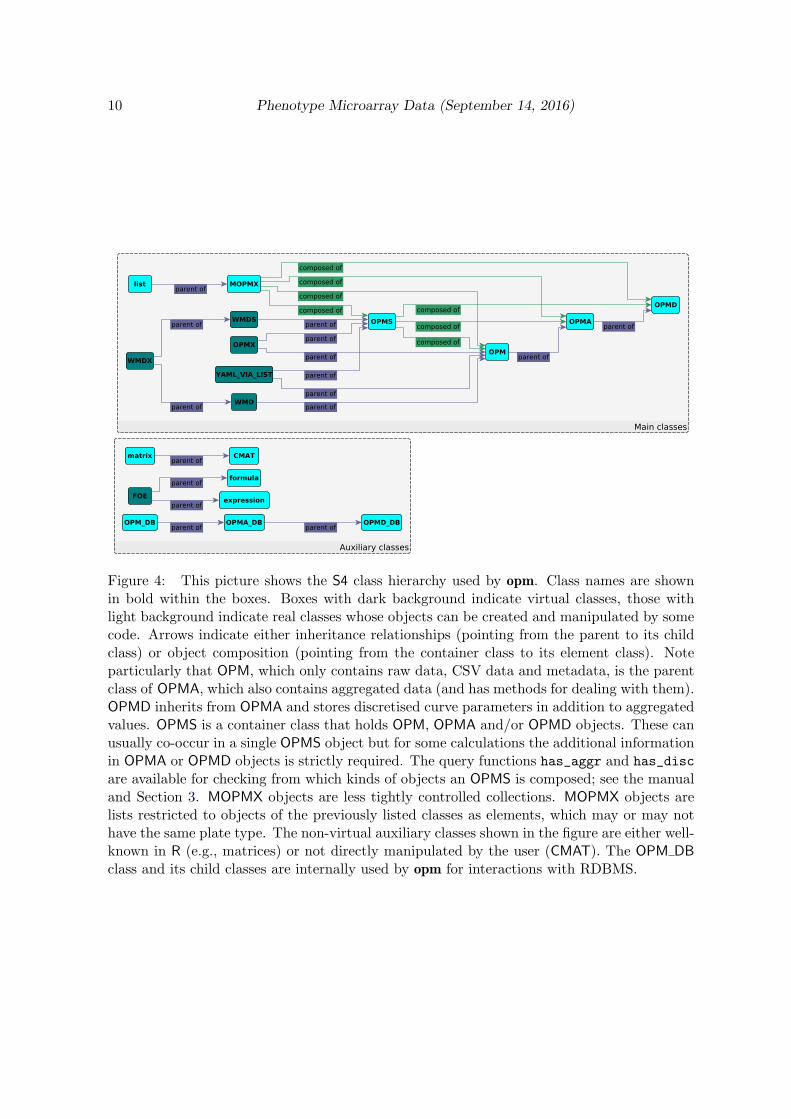
Figure 4: This picture shows the S4 class hierarchy used by opm. Class names are shownin bold within the boxes. Boxes with dark background indicate virtual classes, those withlight background indicate real classes whose objects can be created and manipulated by somecode. Arrows indicate either inheritance relationships (pointing from the parent to its childclass) or object composition (pointing from the container class to its element class). Noteparticularly that OPM, which only contains raw data, CSV data and metadata, is the parentclass of OPMA, which also contains aggregated data (and has methods for dealing with them).OPMD inherits from OPMA and stores discretised curve parameters in addition to aggregatedvalues. OPMS is a container class that holds OPM, OPMA and/or OPMD objects. These canusually co-occur in a single OPMS object but for some calculations the additional informationin OPMA or OPMD objects is strictly required. The query functions has_aggr and has_disc
are available for checking from which kinds of objects an OPMS is composed; see the manualand Section 3. MOPMX objects are less tightly controlled collections. MOPMX objects arelists restricted to objects of the previously listed classes as elements, which may or may nothave the same plate type. The non-virtual auxiliary classes shown in the figure are either well-known in R (e.g., matrices) or not directly manipulated by the user (CMAT). The OPM DB
class and its child classes are internally used by opm for interactions with RDBMS.

M. Goker, B. Hofner, M.d.C. Montero Calasanz, J. Sikorski, L.A.I. Vaas 11
making use of multiple-core machines.
2.4. Integration of metadata
Metadata are “data about data”. They can be either structural, i.e. indicating the waydata are stored, or descriptive, i.e. providing background information on the content of thedata. In the case of PM data, such descriptive metadata can include all kind of describingcharacteristics of the observed organisms such as taxonomic affiliation, geographical and/orecological origin, and of the performed experimental setting such as culture conditions, geneticmodifications, physiological information of any kind and so on.
The interface of the Data Collection software of the OmniLog➤ reader is restricted in sizeand contains only comparatively few fields for entering accompanying information to eachplate such as on the organism under study or the culture conditions. Further, not all of thesefields are exported together with the raw measurements. The few metadata that come alongwith the imported CSV file can be accessed via csv_data. But for most experimental designsit is clearly necessary to add much more meta-information to the kinetic data. It might alsohappen that the metainformation from CSV files is not only limited but also inconsistent oreven erroneous, depending on what has been entered into the OmniLog➤ instrument.
The opm user can integrate the metadata into OPM and OPMS objects using functions suchas include_metadata (see Section 3.1). Often the metadata are kept in a data frame whichcan conveniently be saved to, and generated directly from, a CSV file. How to safely editsuch a file with Microsoft Excel is shown in Figure 5. For an unambiguous match between theraw kinetic data in the OPMS object and the collected metadata, a unique Identifier (ID) isneeded. This is, by default, provided by the combination of Setup Time and Position, whichshould unequivocally identify certain plates. Setup Time indicates the date and time at theprecision of seconds of starting the batch read in the OmniLog➤ reader. Position indicatesthe position of the plate in the OmniLog➤ reader. (For instance, 10-A indicates the platesliding carriage number 10 in slot A of the reader, but for opm the meaning is irrelevant, asthese entries only serves as ID.) Both Setup Time and Position are automatically recordedby the OmniLog➤ reader Data Collection software and are exported by the OmniLog➤ PMFile Management/Kinetic Analysis software into CSV files together with the raw kinetic data.
To ease the manual compilation of metadata, collect_template generates a data frame (andadditionally, if requested, a CSV file) in which each line represents a single PM plate. Thefunction collect_template by default automatically includes the Setup Time and Positionof each plate into the data frame or file providing a structured template for the addition ofmetadata. The user can subsequently add further columns describing any metadata of intereston any PM plate of interest. The resulting data frame can then be queried for the informationspecific to each plate, and the corresponding row integrated into OPM or OPMS objects usinginclude_metadata. Whereas this function will usually result in non-nested metadata entries,opm allows one, in principle, to deal with arbitrarily nested meta-information. This holdsbecause within OPM or OPMS objects metadata are not stored as data frames and notorganised into rows and columns. The amount of meta-information added (and the numberplates simultaneously analysed) is only limited by the available computer memory. Functionsfor generating and modifying plate meta-information are listed in Section 3.1.
The user can provide additional information to the metadata data frame on the fly by callingthe function edit, which opens the R editor enabling the user to modify and add data. More-

12 Phenotype Microarray Data (September 14, 2016)
Upper left: choose the column to be split.Upper right: select tabulator as separator.Lower left: set resulting columns to mode text.Lower right: enjoy the result.
Figure 5: When using Microsoft Excel for editing metadata template files exported by opm,care must be taken that these files remain interpretable by opm. After exporting a file inCSV format under default settings and opening that file with Microsoft Excel, the entries willnot be split into separate columns. To fix this, mark the single existing column and choosethe Text to Columns tool. Select the tabulator as column separator and set all columns (atleast the “Setup Time” column) to Text as Column data format. After clicking Finish thecolumns should then appear correctly. Further columns can then safely be added and the filesaved, but make sure it is saved in CSV format instead of the native Microsoft Excel format.Afterwards the file can be input by opm again as described in Section 3.4.

M. Goker, B. Hofner, M.d.C. Montero Calasanz, J. Sikorski, L.A.I. Vaas 13
over, you can just assign the metainformation from the CSV files to the metadata in one line ofcode. As an alternative to changing the metadata entries by using the R editor, map_metadatasafely maps metadata within OPMS objects. The replacement function metadata<- enablesthe user to set the entire meta-information, or specific entries, directly. If a data frame isused on the right side of the assignment whose number of rows is identical to the number ofplates within the OPMS object on the left side, each data-frame row is specifically added tothe corresponding plate. Note that LIMS input automatically yielded metadata entries.
There are no restrictions regarding the stored metadata values but it usually makes notmuch sense to store factors. It is safer to store character vectors instead because conversionsotherwise might easily result in integer vectors instead of factors. Where appropriate, factorswould be created on-the-fly from character vectors by those methods that have to integratemetadata into data frames. A map_metadata method is available that conducts an accordingcleaning of metadata entries. With respect to the stored metadata names, there are onlyvery few restrictions, which are explained in Section 2.13. In contrast to data frames it is notadvisable to access metadata entries by position instead of by name.
2.5. Aggregating data by estimating curve parameters
The function do_aggr calculates descriptive curve parameters from the kinetic raw data viaspline-fitting and includes them in OPM and OPMS objects. (Extraction of curve parametersthrough the fit of sigmoid functions proved for several PM curve shapes to yield biologicallyunrealistic values (Vaas et al. 2012) and have therefore not been implemented.) Three differentmodelling alternatives for the splines exist (Vaas et al. 2013a): (low-rank) cubic smoothingsplines (Reinsch 1967) as implemented in smooth.spline from the base package as well asthin-plate splines (Wood 2003, a generalisation of smoothing splines) and P-splines (Eilers andMarx 1996) as provided by the package mgcv. Their settings have been specifically adapted toPM data. This worked less well for smoothing splines than for thin-plate splines and P-splinesbecause a tendency of smoothing splines remained to overfit the data. It is also possible toaccess methods from the package grofit (Kahm, Hasenbrink, Lichtenberg-Frate, Ludwig, andKschischo 2010) or to use a native implementation which is faster but only estimates two ofthe four parameters. It is nevertheless recommended to use the default, successfully optimisedspline method.
The descriptive curve parameters lag phase (λ), respiration rate (µ), maximum curve height(A) and Area Under the Curve (AUC) estimated by opm are shown in Figure 6. In addition tothe point estimates for the parameters from both model and spline, their confidence limits canbe calculated (for the spline-based approach via bootstrapping), with 95% being the defaultvalue (Efron 1979). But confidence intervals and according group means can also, and usuallyshould, be calculated from experimental repetitions, as explained in Section 2.8. Attachingthe aggregated data to an OPM object yields an object of the class OPMA, which can also bestored within an OPMS container object.
2.6. Manipulation of OPM and OPMS data
As usual, data analysis starts with data exploration (Section 3.1). It is easy to select specificwells and time points from OPM or OPMS objects. It also straightforward to select specificOPM objects from an OPMS object that contains them. To this end, OPM and OPMS
methods for the generic function subset and R’s bracket operator have been implemented.

14 Phenotype Microarray Data (September 14, 2016)
Time
Valu
e
lag (λ)
slope (
µ)
area under the curve (AUC)
max (A)
Figure 6: A schematic depiction of a typical respiration curve and the parameters estimatedby opm. (Growth curves could be described in the same way.) The descriptive curve pa-rameters are λ, µ, A and AUC. Note that many respiration curves, even if representing aclearly positive reaction, do not correspond to this idealised scheme. The parameters cannevertheless be robustly estimated from deviating curves, particularly via spline fits (Vaaset al. 2012, 2013a).
Particularly powerful are the options for metadata-based creation of subsets. These permitqueries for the presence of a specific metadata key or a specific value of a specific metadatakey, or a specific combination of values and/or keys, and allow for creating according subsetsof OPMS objects.
A plethora of methods for querying other aspects of OPM and OPMS objects have also beenimplemented, as well as standard operations such as sorting objects and making them unique.It is also possible to build up larger OPMS objects by combining OPMS and OPM objectsusing specialised methods for the c generic function and the + operator as well as the veryflexible function opms. Moreover, an OPMS method for merge has been implemented, whichallows for concatenating PM measurements that represent subsequent runs of the same plate.This has successfully been applied to slow-growing organisms in the bacterial genus Geoder-matophilus, which had to be measured three times consecutively in the OmniLog➤ instrument(up to twelve days in total) (Montero-Calasanz, Goker, Potter, Rohde, Sproer, Schumann,Gorbushina, and Klenk 2012; Montero-Calasanz, Goker, Rohde, Schumann, Potter, Sproer,Gorbushina, and Klenk 2013).
It is also possible to convert OPM or OPMS objects to other objects for an independentexploration by the user. This can be done within R, based on a variety of distinct data-frameor matrix objects that can be generated. Alternatively, export in some useful file formats ispossible.
2.7. Plotting functions for raw data
The function xy_plot displays the raw measurements on the y-axis in dependency on the

M. Goker, B. Hofner, M.d.C. Montero Calasanz, J. Sikorski, L.A.I. Vaas 15
time on the x-axis.
For each well one sub-panel is drawn, and the user is free to colourise the plotted curves byeither their affiliation to a specific plate or by a combination of metadata entries of choice.By default the panels are arranged according to the factual microtiter plate dimensions (eightrows labelled A to H × twelve columns labelled 01-12), but other user-defined arrangementsare easily feasible because specific wells can be selected. Every panel is annotated with themicrotiter plate numbering (A01 to H12) and additionally or alternatively with the substratename (given the plate type, the opm package can translate all well coordinates to substratenames, see also vignette “Working with substrate information in opm”). Thus, the functionenables the user to compare the curve data in a customised and useful arrangement (Vaaset al. 2012, 2013a).
Since the estimation of curve parameters (see Section 2.5 and (Vaas et al. 2012)) is alleviatedin the case of curves from finished reactions, we strongly recommend to also use xy_plot forassessing whether or not measurement times had been exhaustive and respiration reactionswere completely recorded. A clear indication of not exhaustively recorded experimental runsis usually the absence of a final plateau phase in the recorded curves.
A statistical test for the completeness of respiration measurements over time is not known tous, but it should be easy to visually identify finished reactions. Nevertheless, some experi-mental experience is necessary to determine minimum running times for the organisms understudy. But plates with slowly reacting organisms can subsequently be measured several timesand the results put together using the merge method.
Depending on the question under study, it may or may not be advisable to further processcurve parameters estimated from unfinished reactions. Experimenters should keep in mindthat conclusions can only be drawn from recorded data. The part of a curve that is notmeasured remains unknown, which might obscure existing differences. Moreover, parameterssuch as A might not always be biologically interpretable as usual when inferred from unfinishedreactions. Since it increases constantly with increasing measurement times, AUC can only becompared between curves with the same overall running time. But the subset method forOPMS objects can easily reduce a set of plates to the time points common to all of them,which would avoid comparing apples and oranges.
The function level_plot provides false-colour level plots from the raw respiration measure-ments over time. Each respiration curve can be displayed as a thin horizontal line, in whichthe measured respiration value (in OmniLog➤ units) is represented by colour, while the x-axes indicates the measurement times. With increasing respiration measurement values, thedisplayed colour changes (by default) from light yellow into dark orange and brownish. Theuser can obtain an overview in a compacted design (Vaas et al. 2012, 2013a). This displayformat is especially powerful for uncovering general differences between plates, for examplelonger lag phases or smaller AUC values across the majority of wells. By default one sub-panelin the level plot corresponds to one complete plate comprising 96 lines, but as in the case ofxy_plot plotting could also be preceded by creating subsets of the plates.
2.8. Plotting the aggregated data
For the graphical representation of the aggregated data the opm package provides four differ-ent functions, namely parallel_plot for visualising distinct curve parameters in one plot aswell as radial_plot, ci_plot and heat_map for displaying a selected curve parameter.

16 Phenotype Microarray Data (September 14, 2016)
parallel_plot provides an overview of at least two estimated parameters and visualises theirinterrelationships. Such a parallel coordinate plot produces an effective graphical summaryof a multivariate data set when there are not too many variables. Since the variables areautomatically scaled to a fixed range, this is equivalent to working with standardised values.This is important for PM data because the distinct curve parameters are measured on quitedifferent scales.
radial_plot displays a plot of radial lines, polygons or symbols, or a combination of these,centred at the midpoint of the plot frame, the lengths, vertices or positions corresponding tothe numeric magnitudes of the data values.
ci_plot displays point estimators and corresponding confidence limits for the depicted curveparameters of selected curves. Thus the characteristics of different curves assembled intoa single overview facilitates the interpretation and comparison of user-defined data subsetsarranged according to the technical and/or biological repetition structure or other aspects ofthe experimental design (Vaas et al. 2012).
Additionally, the package can plot the aggregated curve parameters as a heat map. Heatmaps appear particularly powerful for visualising the outcomes of PM experiment becausedendrograms inferred from both the substrates and the plates can be used to rearrange theplot. Since the user is free to define the metadata to be used for the annotation of the plot andthe clustering analysis, the function heat_map is powerful for data exploration in specialisedcontexts. For instance, the naming scheme of the individual plates can be devised by selectingassociated metadata. It is also possible to automatically construct row groups by selectingthe same or other meta-information.
Further, opm can plot aggregated values as radial plots using an eponymous function, whichis mainly a wrapper for the radial.plot function from the plotrix package adapted to thetypical opm objects. heat_map is mainly a wrapper for the heatmap functions from eitherthe stats or the gplots R package, but contains some useful adaptations to PM data. Itfacilitates the selection of a clustering algorithm and the construction of row and columngroups, and provides more appropriate default solutions for row and column descriptionssizes. (We suppose that in most situations the pictures produced by heat_map should notneed to be manually adapted in these respects.)
2.8.1. Normalisation of aggregated curve parameters
When analysing empirically obtained measurements such as PM data it is important to con-sider possible systematic variations and to control for those by normalisation. For a PMexperiment the purpose of such a normalisation is to minimise systematic variations in theaggregated curve parameters so as to more easily recognise biological differences, as well as toallow for the comparison of parameters across plates processed in different experimental runs.The underlying ideas are mainly derived from DNA-microarray experiments for measuringgene-expression levels (Quackenbush 2002).
Using extract the user can select certain aggregated or discretised values into common ma-trices or data frames. If applied a second time to a previously generated data frame, extractcan compute point estimates and their respective confidence intervals for individually de-fined experimental groups. Optionally, normalisation by subtracting, or dividing through,the plate-wise means (across all 96 wells) or well-wise means (across all plates that containthis well) can be conducted beforehand. Although this method is intended mainly as a helper

M. Goker, B. Hofner, M.d.C. Montero Calasanz, J. Sikorski, L.A.I. Vaas 17
function for ci_plot, it can be quite useful for specific normalisation purposes, for examplewhen data were derived before and after servicing the OmniLog➤ facility, which might resultin shifting the measurements by a certain amount. In conjunction with extract, ci_plotallows for visualising point estimates and confidence intervals of groups of parameter esti-mates. For visualising differences between groups and their confidence intervals, see opm_mcpas described in Section 2.9.
2.9. Statistical comparisons of group means
Besides comparing single curves, the user may also be interested in statistically comparing themean values of distinct groups of curves. For example, imagine the comparison of four differentbacteria using GEN-III micro-plates. For instance, assume that for each bacterial strain, tenreplicates have been performed. (An according example data set is actually available in theopmdata package.) Do these four bacteria differ in the mean value of curve parameter A ofwell A01? Here, a statistical comparison of four groups (four organisms), each containingten values (curve parameter A of 10 replicates of well A01), would need to be performed.Statistically, this requires simultaneous inferences across multiple questions (Hothorn, Bretz,and Westfall 2008).
To address this issue the function opm_mcp performs simultaneous multiple comparisons ofgroup means by internally calling glht from the multcomp package (Hothorn et al. 2008)but providing an easier interface for it, specifically adapted to the typical objects used withinopm. By referring to available metadata and/or the substrate names, the user can definegroups of interest, set up a model of choice and perform multiple comparison of group meanson individually specified contrasts (Bretz et al. 2010; Hsu 1996). The choice of appropriatemodels and contrasts will be explained in detail below. As comparisons of the different curveparameters are performed separately, it is possible to ask very specific questions on differencesbetween curve shapes.
At this point, it is necessary to highlight the power and flexibility of simultaneous multiplecomparison procedures and to encourage the user to apply contrast tests on individuallydesigned sets of mean comparisons rather than to employ the probably more popular classicalAnalysis Of Variance (ANOVA) approaches, which perform F-tests. In general, such F-testsonly provide global information about main effects and interaction effects. That is, onlythe significance of a result yields evidence for a difference in the means among any of theconsidered treatments. For example, in the framework of PM data, a significant F-test onthe effect of the substrate would indicate that at least two of the substrates cause distinctrespiration. Considering that each PM experiment encounters up to 96 different substratesper plate (overall up to 2,000), this information would, obviously, be nearly useless. Moreover,F-tests neither provide information about effect sizes nor do they ease addressing comparisonsof particular interest (Schaarschmidt and Vaas 2009).
We thus opine that most underlying questions in PM experiments are best expressed as a setof particular mean comparisons, resulting in a multiple-comparison problem (Hochberg andTamhane 1987). However, if an increasing number of hypotheses is tested, with the number oftrue hypotheses unknown, the probability of at least one wrong testing decision also increases.That is, if an increasing number of groups is compared to each other, conclusions on significantdifferences between a pair of groups are increasingly likely to be wrong. Thus the so-calledfamily-wise error-rate, which is essentially the probability of at least one false rejection among

18 Phenotype Microarray Data (September 14, 2016)
all the null hypotheses, needs to be controlled (Tukey 1994). The here employed functionsfrom the package multcomp solve all those difficulties, since they allow for testing a user-defined set of contrasts based on a broad range of model types while internally controllingthe family-wise error-rate.
Users of multiple-comparison procedures, especially of simultaneous multiple contrast tests asapplied here, are encouraged to have a look into the books by Hochberg and Tamhane (1987)and Hsu (1996). Regarding the important topic of sample size estimation and power compu-tation, we here provide a brief overview and recommend to further consult textbooks such asSokal and Rohlf (1995) and Zar (1999). The aim of a statistical test is to determine whetheror not there is a significant difference between the observed group means. An appropriatesample size depends on the following parameters:
❼ The desired statistical power and the corresponding significance level α.
❼ Whether or not the test is planned as one- or two-sided comparison.
❼ The minimum expected difference, also called the effect size.
❼ The estimated measurement variability.
The crucial issue regarding sample size is its effect on the statistical “power”. The power of astatistical test is defined as the probability that the test correctly rejects the null hypothesiswhen the alternative hypothesis is true. In a false-negative result, the test does not rejectthe null hypothesis even though there is a difference; this behaviour is referred to as “type-IIerror”. A larger sample size increases the power and reduces the frequency of type-II errors(Eng 2003). Unfortunately, power is directly influenced by the significance criterion α: forsmaller values of α, a larger sample size is needed to obtain a certain power. Similarly, theminimum expected difference between two groups influences the necessary sample size: Thesmaller the effect size, the higher the sample size needed to maintain a given power. Finally,a larger variability of the samples increases the sample size needed to detect a minimumdifference. Power calculations in R can be done using functions in the package pwr (Champely2012) or using the function power.t.test from the stats package.
Especially in situations where groups are defined by more than a single metadata entry theevaluation of differences of treatment means may result in quite complex models. Then,the application of cell-means models (also known as pseudo-one-way layouts) as discussedin (Schaarschmidt and Vaas 2009)) is strongly encouraged. In this approach estimators fortreatment and variance are derived from a model with all treatments combined into a singlefactor. Technically, this requires the merging of several defining metadata variables into asingle one. This can be done by creating new metadata entries from given ones and storingthem back in an OPM or OPMS object. An according example is given in Section 3.4.Alternatively, merging can be done when selecting metadata for creating data frames. Thecomputation of multiple comparisons using a cell-means model is shown in Section 3.9.
The function opm_mcp internally reshapes the data into a “flat” data frame containing onecolumn for the chosen parameter value, one column for the well (substrate) name and op-tionally additional columns for the selected metadata. For performing the testing procedure,a model has to be stated that specifies the factor levels that determine the grouping (Searle

M. Goker, B. Hofner, M.d.C. Montero Calasanz, J. Sikorski, L.A.I. Vaas 19
1971; Hothorn et al. 2008). The opm_mcp function allows for applying such testing directly toOPMS objects, obtaining these factors from stored metadata.
Albeit unusual, depending on the individual study design, the underlying experimental ques-tion and/or the used plates, it might be necessary to perform multiple tests and confidence-interval estimations for ratios of means (e.g., “fold changes”) rather than differences of means.A demonstration of those applications is beyond the scope of this vignette, but the reshapingof the data implemented in opm_mcp provides a ready-to-use input format for test compu-tation. For R the necessary functions are available in mratios (Djira, Hasler, Gerhard, andSchaarschmidt 2012) and SimComp (Hasler 2012b). A valuable overview on the mathemati-cal background is provided by Dilba, Bretz, and Guiard (2006), whereas examples for specialapplications can be found in Hasler (2012a).
2.10. Discretising the aggregated data and export for phylogenetic analysis
Whereas the main data-analysis strategies of the opm package are based on quantitative,continuous data (as described in the previous chapters), users may nevertheless be interestedin discretising the estimated curve parameters. Discretisation transfers continuous data intodiscrete ones. For example, continuous values ranging from 0 to 400 could be discretised intothe three states“low”(from 0 to 100),“intermediate”(from 101 to 200), and“high”(from 201 to400). Discretising the data is necessary for analysing them with external programs that cannotdeal with continuous characters. Indeed, phylogeny software such as PAUP* (Swofford 2003)and RAxML (Stamatakis, Ludwig, and Meier 2005) is limited to at most 32 distinct characterstates. (To the best of our knowledge, a maximum-parsimony algorithm applicable directlyto continuous data has only been implemented in TNT (Goloboff, Farris, and Nixon 2008).)Phylogenetic studies of PM data, or at least reconstructions of PM character evolution, areof interest because such phenotypic information is frequently used for taxonomic purposesin microorganisms, and here phylogenetic inference methods might be superior to clusteringalgorithms (Felsenstein 2004). But tabular or textual descriptions of physiological reactionsclassified into negative, weak (ambiguous) and positive reactions (see Section 2.11 for details)are of even greater relevance in current microbial taxonomy (Tindall, Kampfer, Euzeby, andOren 2006).
The opm package includes data transformations (implemented in the discrete methods)for coding continuous characters by assigning them to a given number of equal-width cat-egories within a given range. For example, for the parameter A the theoretically possiblerange between 0 and 400 OmniLog➤ units could be used. The data should then be analysedunder ordered (Wagner) maximum parsimony in PAUP* (Farris 1970) or with the optionsfor ordered multiple-state phenotypic characters in RAxML (Berger and Stamatakis 2010),or corresponding settings in other programs, to minimise the loss of information caused bydiscretising the values. For this reason, this kind of unsupervised, equal-width-intervals dis-cretisation (Dougherty, Kohavi, and Sahami 1995; Ventura and Martinez 1995), even thoughsimple, appears appropriate for this task. In this context, it also makes not much sense tolet a discretisation method determine the number of categories because they are not dictatedby some property of the data but by the limitations of the subsequently to apply analysissoftware. opm can appropriately export discretised data.
2.11. Determining positive and negative reactions and displaying them as

20 Phenotype Microarray Data (September 14, 2016)
text or table
If users wanted to discretise the parameters into “positive” and “negative” results, this wouldapparently make most sense for the parameter A because here it is not of interest when andhow fast a reaction starts (which would be coded in λ and µ, respectively) or how muchoverall respiration was achieved (as coded in AUC) but whether or not a reaction takes placeat all. Unfortunately, PM data frequently result in a continuum of A values between clearlynegative and clearly positive reactions. For instance, the distribution of A in the exampledata sets distributed with the opm and opmdata packages is obviously bimodal, but containsa large number of intermediary values. For this reason, do_disc implements a gap-modediscretisation by interpreting a given range of values (within the overall range of observations)as “ambiguous”. Values below would then be coded as negative, values above the range aspositive, and values within the range as either missing information or an intermediary state,“weak”.
This range could be determined by some discretisation approach known from the literature(Dougherty et al. 1995; Ventura and Martinez 1995). The opm package can automaticallydetermine it using k-means partitioning as implemented in Ckmeans.1d.dp (Wang and Song2011), using an exact algorithm for one-dimensional data. Alternatively, an algorithm im-plemented in best_cutoff is available, but it requires measurement replicates (which arehighly recommended, if not mandatory, anyway) accordingly annotated in the metadata.Both methods are accessible via do_disc, too.
Export as richly annotated, publication-ready Hypertext Markup Language (HTML) table ortext is possible using phylo_data and listing. If analysis with phylogenetic programs wasof interest, in the case of an intermediary state the data should then be analysed as describedabove. If intermediary values were coded as missing information they could be analysed undereither Wagner or unordered (Fitch) maximum parsimony in PAUP* (Farris 1970; Fitch 1971)or with the options for binary phenotypic characters in RAxML (Berger and Stamatakis 2010),or corresponding settings in other programs.
2.12. Database input and output
This topic is for advanced users and bioinformaticians, as it requires setting up, or at least hav-ing access to, a database server. For this reason, automatically executed (and thus checked)code for database I/O of PM data directly within R can neither be included here nor in theexample sections of the opm manual. We have, however, tested all of the following state-ments, and all of the mentioned code examples, on our own workstations. But for a successfuldatabase interaction users might need information that is not directly related to opm and thuscannot be treated in the documentation of this package. We can nevertheless provide examplecode that uses opm together with database-specific R packages for storing and receiving PMdata.
Database interaction differs greatly depending on whether a relational database or one ofthe more recent NoSQL alternatives is concerned. For working with a Relational DatabaseManagement System (RDBMS), a scheme needs to be defined beforehand for storing thePM data, and additional conversions and selections are necessary. The scheme requiredby the opm_dbput function and its accompanying functions such as opm_dbget is providedwith opm via opm_files("sql"). Whereas these functions require certain column names, aswell as inter-table relationships defined by foreign keys, the tables could be renamed. Note

M. Goker, B. Hofner, M.d.C. Montero Calasanz, J. Sikorski, L.A.I. Vaas 21
particularly that columns for the metadata of interest could (and usually should) be addedto the “plates” table. Call demo(package = "opm") to see examples for SQLite, MySQL andPostgreSQL. This code was successfully tested locally with RSQLite (James, Falcon, andthe authors of SQLite 2013), RMySQL (James and DebRoy 2012), RPostgreSQL (Conway,Eddelbuettel, Nishiyama, Prayaga, and Tiffin 2013) and RODBC (Ripley and from 1999 toOct 2002 Michael Lapsley 2013).
A popular document-oriented database is MongoDB, which is accessible via the RMongo
package (Chheng 2013). If you have set up a local MongoDB server and installed RMongo,call demo("MongoDB-IO", package = "opm") for a usage example. The data storage usedwithin opm fits well to a document-oriented database because OPMX objects do not enforcea particular structure for storing the metadata (see Section 2.4). The same holds for the“options” entries of the aggregation and discretisation settings.
Finally, the output YAML format (or its subset, JSON) is likely to facilitate the quick estab-lishment of third-party software for importing PM data into a database (Caspi et al. 2016).
2.13. Global settings
It is possible to modify settings that have an effect on multiple functions and/or on frequentlyused arguments globally using opm_opt. This allows the user to adopt opm to personalpreferences and to thereby substantially decrease coding effort. It is checked that the novelvalues inherit from the same class(es) than the old ones. Usage examples are provided inseveral sections (e.g., Section 3.10.3).
The function param_names yields the spelling of the curve parameters used by opm. It alsodisplays the set of names that are used by some methods that have to compile metadataentries with other columns. It is thus not impossible, but discouraged, to use these namesas metadata keys. The same holds for (non-syntactical) names starting with an underscoreand followed by capital letters, as such names are temporarily used by some methods inintermediary objects together with the metadata.
3. Program application
3.1. Overview
The most important functions that can be used in each step of the possible opm work flowsare shown in Figure 7. For a complete list of user-level functions see the manual.
Before starting, the opm package should be loaded into an R session as follows:
R> library("opm")
The example data set distributed with the package (Vaas et al. 2012) comprises the re-sults from running 114 GEN-III plates (BIOLOG Inc.) in the PM mode of the OmniLog➤reader. The organisms used were two strains of Escherichia coli (Deutsche Sammlung vonMikroorganismen (DSM) 18039 = K12 and the type strain DSM 30083T) and two strainsof Pseudomonas aeruginosa (DSM 1707 and 429SC (Selezska, Kazmierczak, Musken, Garbe,Schobert, Haussler, Wiehlmann, Rohde, and Sikorski 2012)). The strains with a DSM number

22 Phenotype Microarray Data (September 14, 2016)
Previously generated YAMLRaw data (CSV file)
Input via read_opm
compile metadata via editing a data frame in R
or a CSV file with a spreadsheet software
generate metadata template for OPM or OPMS
objects via collect_template
combine usingopms,c, +,[ ]<-
raw kinetic data
raw kinetic and aggregated data
raw kinetic, aggregated and discretized data
OPM
OPMA
OPMD
OPMS
OPMS
OPMS
raw kinetic data
raw kinetic and aggregated data
raw kinetic, aggregated and discretized data
aggregate via do_aggr
discretize via do_disc
aggregate via do_aggr
discretize via do_disc
single plate
add metadata via include_metadata
Init
ial
co
mp
ila
tio
n o
f d
ata
Data containers flexibly compiled according to the interests and needs of the user
output YAML, CSV, etc.:to_yaml/write,as.data.frame/write.table,phylo_data/write
manage metadata:metadata<-,include_metadata,map_metadata,metadata_chars
create plots:level_plot,xy_plot,ci_plot/extract, heat_map, radial_plot, annotated,parallelplot
query metadata and select:subset, [ ],%k%, %q%, %K%, %Q%
convert:flatten,extract,opm_mcp
OPM, OPMA, OPMD, OPMS objects
Single to many plates with raw kinetic and metadata, and optionally aggregated and discretized data
conduct multiple comparisonof means:opm_mcp
Da
ta a
na
lys
is a
nd
ma
na
ge
me
nt
create tables and/or text:phylo_data, listing
obtain basic information:summary,metadata,aggregated,discretized,...
explore data within R yourself
publish tables
and/or text
exploredata
elsewhere
publish figures
Data frame
Conversion via opmx
many plates
publish statistics
read from and/or write to databases:opm_dbput,opm_dbget,...
use database storage
Figure 7: Overview of the possible strategies and appropriate functions for data analysisusing the opm package. Beginning with one to several CSV files containing raw kineticdata exported by the proprietary OmniLog➤ software File Management/Kinetic Analysis,or YAML or JSON files that have been generated in previous opm runs, OPM or OPMS
objects can easily be generated. Methods for metadata management, plotting the data in acustomised manner, querying and sub-setting the generated objects, statistical comparison ofmultiple group means, and data-conversion tools including discretisation, report generationand output in files are provided. How to use annotated to produce graphics is explainedin the tutorial on substrate information in opm. The input of growth-curve data, or anyother data that have neither been measured with an OmniLog➤ nor a with a MicroStation➋system, is described in the tutorial on analysing growth curves and other user-defined data.As shown in the upper left part of the figure, it only requires the creation of a data framethat can be converted with the opmx function.

M. Goker, B. Hofner, M.d.C. Montero Calasanz, J. Sikorski, L.A.I. Vaas 23
could be ordered from the Leibniz Institute Deutsche Sammlung von Mikroorganismen undZellkulturen (DSMZ) (http://www.dsmz.de/).
Each strain was measured in two biological replicates, each comprising ten technical replicates,yielding a total of 80 plates. To additionally investigate the impact of the growth age ofthe cultures on the technical and biological reproducibility of the PM respiration kinetics,strain E. coli DSM 18039 was grown on solid Lysogeny Broth (LB) medium for nine differentdurations, from 16.75 h (t1 ) to 40.33 h (t9 ), respectively. For each growth duration fourtechnical replicates were performed except for t9 (which was repeated only twice), yielding34 plates for this time-series experiment. All biological and experimental details of this dataset have been described previously (Vaas et al. 2012).
Two subsets of the data, vaas_1 and vaas_4, are included in opm. See their description inthe manual, and have a look at the objects as follows:
R> vaas_1
R> vaas_4
The entire data set, stored in the object vaas_et_al, comes with the supporting packageopmdata and can (if that package is installed, of course) be loaded using:
R> data(vaas_et_al, package = "opmdata")
The metadata included in these objects comprise seven entries, as described in the opmdata
manual. The entry Experiment denotes the biological replicate or the affiliation to the time-series experiments. The keys Species and Strain refer to the organism used for the respectiveexperiment (see above), and Slot (either A or B) indicates whether the plate was placedin the left or the right half of the OmniLog➤ reader. (Note that for an assessment of thereproducibility of the curves the slot is occasionally of relevance.) Two additional entriescontain the index of the time point and the corresponding sample point in minutes for thetime series experiment. The key Plate number indicates the technical replicate (per biologicalreplicate). The combination of the keys Strains, Species, Experiment and Plate number resultsin a unique label which unequivocally annotates every single plate.
3.1.1. Troubleshooting
It is hard to provide a general hint regarding problems with R code except for the followingone: If anything fails, read the issued error message and take it serious.
3.2. Data import
The following code illustrates the import of the OmniLog➤ CSV file(s) into the opm package.In the opm manual and all help pages, all data import functions are contained in the family“IO-functions” with according cross-references.
The CSV files with the OmniLog➤ raw data should be stored in one to several user-definedfolders. Setting the working directory of R to the parent folder of these using setwd frequentlyfacilitates file selection, but in principle the user can provide any number of paths to inputfiles and/or directories containing such files to the function read_opm, which can load severalCSV files (and also YAML or JSON files generated by opm) at once. A former restriction of

24 Phenotype Microarray Data (September 14, 2016)
the input functions was that they could solely read new-style CSV files that only containedthe measurements from a single plate per file (either a PM plate or a single GEN-III platemeasured in either PM- or identification mode). The function split_files had to be usedto split CSV files with multiple plates into one file per plate, but this is not necessary anymore.
To illustrate the file import step by step, a set of input CSV example files is provided withthe package. Before starting, remember that the opm package must be loaded. Then use thebuilt-in function opm_files to find the example files in your R installation:
R> files <- opm_files("testdata")
R> files
Afterwards check whether this returned a vector of nine file names, including the full path totheir location in the file system. (It might fail in very unusual R installation situations; in thatcase, the files must be found manually.) For demonstration purposes, the test data containEcoPlate➤ Gen-III, PM01 and PM20 plate types. One of these files contains multiple platesand could be used as an example for split_files, but it can also directly be read.
Using read_opm, from a given vector of file and/or directory names, files can easily be selectedand deselected using globbing or regular-expression patterns. For instance, for reading thethree example files in “new style” CSV format (see Section 2.2), use the following code.
R> example.opm <- read_opm(names = files, convert = "try",
include = "*Example_?.CSV.xz")
R> summary(example.opm)
Here convert = "try" causes the function to attempt to combine all input plates in a singleOPMS object. This fails when there are several plate types. (The default is to group byplate type, yielding a MOPMS object, see below.) After performing this step, the OPMS
object contains three plates, as indicated by the summary function. An example for inputtingLIMS-style CSV is here:
R> example.lims <- read_opm(names = files, convert = "try",
include = "*Example_LIMS_*.EXL.xz")
R> summary(example.lims)
R> rm(example.lims)
Instead of a single file name the user could also provide several file names to read_opm, or amixture of file and directory names. If these were contained as subdirectories of the currentworking directory, read_opm(".") or read_opm(getwd) would be sufficient to input thesefiles. To filter the files with patterns, the arguments exclude and include are available. Thereis also a demo mode allowing the user to check the effect of each argument before actuallyreading files. One can use the gen.iii argument to trigger the automated conversion of theplate type to, e.g., GEN-III or “ECO” plates run in “PM”mode, or convert later on using thegen_iii function itself. Plate-type conversions to one of the “PM” modes are disallowed bydefault and are, to the best of our knowledge, hardly relevant in practice anyway. (They wouldonly be necessary if the wrong plate type was entered into the OmniLog➤ instrument.) Theplate type is crucial, as it is disallowed to integrate distinct plate types into a single OPMS

M. Goker, B. Hofner, M.d.C. Montero Calasanz, J. Sikorski, L.A.I. Vaas 25
objects. The reason is that comparing the same well positions from distinct plate types wouldbe almost always equivalent to comparing apples and oranges.
If more than one plate of the same plate type was read, however, data from all files wouldautomatically be integrated into a single OPMS object. To read plates from several types atonce, the convert argument is useful. If one uses read_opm(..., convert = "grp") (thedefault), a named list is created with, as each list element, one OPM or OPMS object per platetype, depending on whether only a single plate of that plate type, or several such plates, havebeen found. For instance, for inputting all example files (except for the one with multipleplates), consider the following code:
R> many.plates <- read_opm(names = files, exclude = "*Multiple*")
R> summary(many.plates)
R> summary(many.plates$PM01)
R> rm(many.plates) # tidy up
This yields the data from plates with distinct plate types in a single object. Note that theobjects for each encountered plate type can easily be accessed via the names of the list. Moreexample code is available via opm_files("demo"). Call demo("multiple-plate-types",package = "opm") after moving to the directory with input CSV files (or a parent directoryof it). Unreadable CSV would yield an error.
A single plate could also be imported using read_single_opm. But this might only occasion-ally be useful, as read_opm can cope with single files, too.
3.2.1. Troubleshooting
A frequent kind of error is that you attempt to read files that are CSV but do not contain PMdata. The name of the first file that fails is shown in the error message, fixing the problemshould thus be straightforward. Use demo = TRUE to first show the files you would read, andif this list contains names of files that expectedly cannot be read by opm, modify the inclusionor exclusion settings. Alternatively, modify your folder structure. Finally, note that you canalways use a character vector of specific file names collected by hand as names argument. Thiswould provide complete control about the files to be read.
The most usual error that occurred with older versions of opm was that it was attemptedto input CSV files with several plates per file, but such multiple-plate CSV files had to besplit beforehand with split_files to generate files that can be input by the package. Thisrestriction has been lifted in current opm versions. Moreover, the most recent versions of theOmniLog➤ software can batch-export one plate per CSV file.
3.3. Batch conversion of many files
In addition to read_opm and read_single_opm (Section 3.2), which need to be called beforean interactive exploration of PM data, batch-processing large numbers of files by convertingthem from CSV (or previously generated YAML or JSON) to YAML, JSON or CSV format,is also possible. This optionally includes aggregating the raw data by estimating curve param-eters (Section 3.5), discretising these parameters (Section 3.10.2) and integrating metadata(Section 3.4). Again there is a demo mode to first investigate the attempted conversions:

26 Phenotype Microarray Data (September 14, 2016)
R> batch_opm(files, include = "*Example_?.CSV.xz",
aggr.args = list(boot = 100, method = "opm-fast"),
outdir = ".", demo = TRUE)
The arguments aggr.args, disc.args and md.args control aggregation, discretisation andmetadata incorporation, respectively. Details on all three processes are given in the accordingsections, and for the exact use of these arguments see the opm manual.
The following command reads three of the seven example input files, estimates two of the fourcurve parameters using the fast native method including 100 rounds of bootstrapping, andstores the resulting YAML files (one per plate) in the current working directory (indicated by"."):
R> batch.result <- batch_opm(files, include = "*Example_?.CSV.xz",
aggr.args = list(boot = 100, method = "opm-fast"),
outdir = ".")
By default, progress messages are printed to the screen. The return value, here assigned tothe batch.result variable, also contains all information about the success of the individualfile conversions.
The run_opm.R script distributed with the package is an Rscript-dependent command-linetool for non-interactively running such file conversions. Its location in the file system can beobtained using
R> opm_files("scripts")
Regarding the use of the script, see the documentation of Rscript (the Rmanual contains an ac-cording entry) and watch the help output of this script (try system(opm_files("scripts"))).
3.4. Integration and manipulation of metadata
Several ways for linking metadata to OPM or OPMS objects are possible. The easiest oneis probably the batch-inclusion after creating a template with plate ID associating it withmetadata. In the first step, either a data frame to be manipulated within R or a CSV file to bemodified with a suitable editor are created. The opm package supports metadata integrationby creating a template for such a table from an OPM or OPMS objects that contains plate IDin the first columns; by default the keys Setup Time, Position and File. These entries mustnot be changed, ensuring that the package can later on link the metadata to the dedicatedplates according to these ID.
In the opm manual and help pages, most metadata-manipulation functions are containedin the family “metadata-functions” with according cross-references. For the collection of ametadata template in a data frame to be manipulated in R, use this command:
R> metadata.example <- collect_template(files, include = "*Example_?.CSV.xz")
For the generation of a metadata template file, the following command can be used:
R> collect_template(files, include = "*Example_?.CSV.xz",
outfile = "example_metadata.CSV")

M. Goker, B. Hofner, M.d.C. Montero Calasanz, J. Sikorski, L.A.I. Vaas 27
This will result in a file "example_metadata.CSV" in the current working directory (whosename is accessible using getwd). If other metadata have previously been collected, by defaultan already existing file with the same name will be reused. The already defined columns willbe respected, novel rows will be added, old metadata will be kept, ID for novel files will beincluded and their so far empty metadata entries will be set to missing data (NA). You can alsoprovide the location of another previously created metadata file with the collect_templateargument previous. An ID for the OmniLog➤ instrument in use can also be added. Thismakes sense if plates from several such machines are analysed. A further option is to normalisethe plate-position and setup-time entries, as described in the manual.
The generated CSV file could then be edited using external software; for the purpose of thistutorial, we load it directly and manipulate it in R. To avoid the usual changes in data formatand header of the table during the import a customised import function was implemented asa wrapper for read.delim:
R> metadata.example <- to_metadata("example_metadata.CSV")
Per default, this expects CSV columns separated by tabulators, with the fields protected byquotes. To input other formats, consider the sep argument for defining an alternative columnseparator, as well as the strip.white argument for turning the removal of whitespace at thebeginning and end of the fields on or off (which is relevant if a spreadsheet program exportsCSV without quotes). Note that you can pass a file name directly to include_metadata. Thisis computationally less efficient but by default the function then tries several strip.whiteand sep arguments in turn unless it succeeds in finding the column names and rows of interest.
Some spreadsheet software might also interpret and reformat the setup time. This needs tobe avoided by declaring the according column to be input as plain text into the spreadsheet,thus preventing any interpretation of its content. See Figure 5 for how to achieve this withMicrosoft Excel.
Now the user could add information to the data frame by calling edit, which would open theR editor, or by any other way of manipulating data frames in R. New columns could be defined,or the existing metadata modified. But the first columns must remain unchanged becausethey are needed to identify individual PM plates for linking them to their meta-information.As an example, we here add an (arbitrary) Colour column with the values “blue”, “red” and“yellow” and another (arbitrary) Integer column with the integer values 10, 20 and 30:
R> metadata.example$Colour <- c("blue", "red", "yellow")
R> metadata.example$Integer <- c(10L, 20L, 30L)
Now the metadata are ready to be included into the previously generated OPMS object:
R> example.opm <- include_metadata(example.opm, md = metadata.example)
The metadata could then be received as follows:
R> metadata(example.opm)

28 Phenotype Microarray Data (September 14, 2016)
This returns the entire metadata entries as a list (for just displaying them, to_metadata(example.opm)is often more convenient, as described below). By default only the added metadata are in-cluded in the object, but not the ID used for assigning data-frame rows to plates.
One might want to remove the metadata CSV file as it is not needed any more:
R> unlink("example_metadata.CSV")
If include_metadata complains about a missing key/value pair, watch carefully whether theshown value contains leading (or trailing) spaces. If so, consider using strip.white = FALSE
when calling include_metadata or to_metadata. The default setting for include_metadatatries several options in turn, however, until the matching succeeds.
A couple of other functions have been implemented for manipulating metadata included inOPM and OPMS objects. For instance, the entire meta-information, or specific entries, canbe set using the replacement function metadata<-. Setting a specific entry named key toa specific value value in all plates is accomplished with metadata(example.opm, key) <-
value. If the right side of the assignment is a data frame with the same length as the OPMS
object, each row would specifically be assigned to the OPM object with the same index. Thismakes it easy to add the selected csv_data, or all information from the OmniLog➤ CSVfiles, to the metadata:
R> metadata(example.opm)
R> metadata(example.opm) <- to_metadata(csv_data(example.opm))[,
c("Strain Name", "Sample Number")]
R> metadata(example.opm)
However, there is an even easier short-cut to copy the csv_data to the metadata:
R> ## do not enter this code, as we already have copied the CSV data
R> metadata(example.opm) <- TRUE # set selected CSV metainformation
R> metadata(example.opm) <- FALSE # remove it again
The csv_data not to be copied (or removed again) are chosen using opm_opt("csv.selection").
You might note that “Sample Number” is a misnomer in these data sets. (One of the fieldsin the interface of the Data Collection software of the OmniLog➤ reader had been de-fined as “Sample Number”, but the operator entered species and strain designations intothis field.) In such cases, modifying the metadata in-place is of use, which is accomplishedwith map_metadata. This function returns a novel OPMS (or OPM) object. Its formulamethod is particularly powerful:
R> metadata(example.opm)
R> metadata(map_metadata(example.opm, Organism ~ ❵Sample Number❵))
This works by converting the left side of the formula into a metadata key and evaluatingthe right side of the formula in the context of the metadata entries that have already beenadded. As result, a new metadata entry is created, with “Organism” as key and the entryfrom “Sample Number” as value. “Sample Number” must be quoted because it contains aspecial character (the blank).

M. Goker, B. Hofner, M.d.C. Montero Calasanz, J. Sikorski, L.A.I. Vaas 29
But we have not yet removed the inadequately named “Sample Number” entries. Here, it isuseful that all operators (except for $ and other high-precedence operators, which can be usedfor defining nested keys) on the left side, if present, are changed by map_metadata into a callto list. The resulting list is flattened and treated as a list of metadata keys. Hence it ispossible to define several keys at once. The right side, once evaluated, is recycled accordingly.Thus we can clean up our metadata in a single line of code:
R> metadata(map_metadata(example.opm,
Organism + ❵Sample Number❵ ~ list(❵Sample Number❵, NULL)))
The deletion of “Sample Number” is accomplished by the assignment of NULL, as usual inR lists. Instead of + almost all other operators could be used, and one could also writec(Organism, ‘Sample Number‘) on the left side, which might be more intuitive. If map_metadatais called without a mapping, it “cleans” the metadata by removing empty entries (by defaultincluding those that only contain NA values) and converting factors to character vectors.
But we have not yet stored an OPMS object with the cleaned metadata. This could be doneusing example.opm <- map_metadata(example.opm, ...). In that case, however, directassignment would also be possible:
R> metadata(example.opm) <- Organism + ❵Sample Number❵ ~
list(❵Sample Number❵, NULL)
R> metadata(example.opm)
Assigning NULL to a metadata entry would remove that entry. We can achieve the same usingan expression object:
R> metadata(example.opm) <- to_metadata(csv_data(example.opm))[,
c("Strain Name", "Sample Number")] # reset
R> metadata(example.opm)
R> metadata(example.opm) <- expression(Organism <- ❵Sample Number❵,rm(❵Sample Number❵))
R> metadata(example.opm)
Here, the assignment targets (names within the metadata) are specified directly using just the<- operator. Apparently, arbitrarily complex code can be put in such a metadata-modifyingexpression.
All metadata are cleared by assigning an empty list, without specifying a key:
R> metadata(example.opm, "Organism") <- NULL
R> metadata(example.opm)
R> metadata(example.opm) <- list()
R> metadata(example.opm)
So keep in mind that formulae and expressions are very flexible for modifying metadata entries.They allow for any other operation (such as numerical calculations) if it can be applied tothe selected predefined metadata content. The replacement function can also be used to copymetadata between OPM and/or OPMS objects.
Metadata can also be assigned specifically for subsets of OPMS objects, using the indexedassignment available for those objects:

30 Phenotype Microarray Data (September 14, 2016)
R> metadata(example.opm[2]) <- list(Organism = "Elephas maximus",
Size = "3 meters")
R> metadata(example.opm)
R> metadata(example.opm[2]) <- list()
R> metadata(example.opm)
You may have noted that metadata always returns a list, not a data frame. This is becausemetadata need not contain the same entries, even within a single OPMS object, and can benested. It is possible, however, to get the metadata as data frame by using to_metadata.Missing entries would then be filled with NA values, and nested metadata entries would yielddata-frame columns of the mode “list”. This might or might not be suitable for furtherprocessing. For statistical analysis, the appropriate way is to extract only those metadataentries that are present in all OPMS elements, and usually also only those that are notthemselves lists. Methods such as extract are based on this principle.
For manual editing, an edit method can directly be applied to OPMX objects, providedthat to_metadata yields a suitable data frame. This is not normally the case unless themetadata are rectangular (in a relaxed sense, as missing values would not matter), which isnot enforced by the way OPMX objects are implemented. So whereas edit might be handyin many situations, one should not expect it to work with all kinds of OPMX objects. If themetadata were unsuitable, it would stop with an error message before any editing by handcan be conducted; otherwise it would (of course) modify the metadata in the intended way.
The following code, making use of the metadata.example data frame generated above, adds anew metadata entry with the key“Character”containing the integer values from the metadataentry called “Integer” converted to character mode. It then includes a new metadata entrywith the key “Times 10” containing the entry “Integer” multiplied by 10.
R> example.opm <- include_metadata(example.opm, md = metadata.example)
R> metadata(example.opm)
R> example.opm <- map_metadata(example.opm, Character ~ as.character(Integer))
R> metadata(example.opm)
R> example.opm <- map_metadata(example.opm, ❵Times 10❵ ~ (Integer * 10))
R> metadata(example.opm)
Note that map_metadata can also be used with character vectors as mapping objects. Makinguse again of the exemplar generated above, the key Colour can be changed to Colony colouras follows:
R> example.opm <- include_metadata(example.opm, md = metadata.example)
R> md.map <- metadata_chars(example.opm, values = FALSE)
R> md.map
This yields a character vector including itself as names attribute, thus implying an identitymapping. In the next step the new labels are defined and then exchanged with the old onesusing map_metadata:
R> md.map["Colour"] <- "Colony colour"
R> example.opm <- map_metadata(example.opm, md.map, values = FALSE)
R> metadata(example.opm)
M. Goker, B. Hofner, M.d.C. Montero Calasanz, J. Sikorski, L.A.I. Vaas 31
The keys have been changed to Colony colour now but the values have remained unaffected.In addition to mapping based on character vectors, a mapping function can also be used. Bysetting their argument values to TRUE, the functions metadata_chars and map_metadata
could be used as well to modify values instead of key. For instance, assume any entries “red”in the field denoted Colony colour should be changed to “green”:
R> md.map <- metadata_chars(example.opm, values = TRUE)
R> md.map
R> md.map["red"] <- "green"
R> example.opm <- map_metadata(example.opm, md.map, values = TRUE)
R> metadata(example.opm)
This command transforms all entries in the table with the value ”red” to ”green”. Othervalues, as well as the keys, are unaffected.
The metadata_chars function can also detect misspellings in metadata name or values if themax.distance argument is set to a non-negative numeric value. It then indicates the upperthreshold for the dissimilarity between two strings to regard them as synonyms. The mostfrequent within each group of strings is regarded as the correct spelling. This is not fail-safe,hence resulting vectors should always be checked before passing them to map_metadata, anddistinct max.distance settings should be tried.
Frequently, metadata entries will be used as factors in statistical models. This always requiresthat the chosen metadata entry is present in all considered OPM object and sometimes requiresthat entries are combined. For instance, for setting up a cell-means model (see Section 2.9and Section 3.9), factors used for defining the groups of interest have to be merged. Thismight already be done during the initial step when setting up the metadata data frame beforeincluding the metadata into an OPM or OPMS object using include_metadata. Here, thefunction interaction could be used to concatenate columns (but it should be taken intoaccount that metadata entries should better not be represented as factors). As a result, twometadata entries would be merged into a single one:
R> # not recommended
R> metadata.example$Colour.Position <-
as.character(interaction(metadata.example$Colour,
metadata.example$Position, drop = TRUE))
This is not advisable, however, unless all statistical comparisons of interest, or at least thegroup definitions of interest, were already known at that early stage. (Even more tediouswould be to go back to the initial metadata compilation in a CSV file.) Using the metadatamapping functions, metadata entries can instead by merged at any time after including theminto an OPM or OPMS object with include_metadata. For instance, the following codeoperates directly in the OPMS object, merging the . “Colony colour” (which had previouslybeen renamed from “Colour”, see above) and “Integer” entries into a new one:
R> metadata(example.opm) <- Col.Int ~ paste(❵Colony colour❵, Integer, sep = ".")
R> metadata(example.opm)
As result, a new metadata entry named“Col.Int”is created with the general string-concatenationtool paste. Note that metadata should not normally contain factors but rather generate themon-the-fly from selected entries, and keep in mind that metadata are not organised in rows.

32 Phenotype Microarray Data (September 14, 2016)
Finally, there is short-cut for assigning a plate ID that is unique during the current opm
session to the metadata:
R> ## do not do this unless you need it
R> metadata(example.opm) <- "ID"
For using keys other than “ID”, use opm_opt("md.id.name"). For resetting the startingpoint, use opm_opt("md.id.start"). If so, keep in mind that all forthcoming IDs might notbe unique any more. You would need to re-assign all of them to ensure uniqueness.
3.4.1. Troubleshooting
The include_metadata function must correctly and uniquely identify plates to correctlyassign the metadata. This cannot work if the identifiers get modified after exporting them.A potential cause for key-value mismatches mismatches is the re-interpretation of date-timeentries (in the column for the setup time) by some spreadsheet software re-interpreting date-time entries. You must set the data type of all columns to text to safely prevent this fromhappening. Consult Figure 5 for how to safely do edit opm metadata template CSV files inMicrosoft Excel.
3.5. Aggregating data by estimating curve parameters
The exemplar OPM object vaas_1 contains a full 96-well plate, aggregated data (curve pa-rameters), and metadata:
R> data(vaas_1)
R> vaas_1
In the opm manual and help pages, the parameter-estimation functions are contained in thefamily “aggregation-functions” with according cross-references. Primarily do_aggr should beused for aggregation because it generates the kinds of objects that allow for the predefinedwork flows. vaas_1 already contains aggregated data but we will now re-estimate parameters.For invoking the fast estimation method, use:
R> vaas_1.reaggr <- do_aggr(vaas_1, boot = 100, method = "opm-fast")
This will only yield two of the four parameters, namely A and AUC. (Screen messages outputby boot.ci might be annoying but can usually be ignored.) The aggregation settings usedcan be accessed via aggr_settings:
R> aggr_settings(vaas_1)
R> aggr_settings(vaas_1.reaggr)
and the aggregated data can be extracted as a matrix via aggregated, e.g.:
R> summary(aggregated(vaas_1))
R> summary(aggregated(vaas_1.reaggr))

M. Goker, B. Hofner, M.d.C. Montero Calasanz, J. Sikorski, L.A.I. Vaas 33
By default do_aggr does not conduct bootstrapping of the kinetic data to obtain confidenceintervals for individual curves because these are not normally needed. As this would be atime-consuming intensive process (particularly if grofit is used), it could be split over severalcores on a multiple-core machine if mclapply from the parallel R package can be run withmore than one core, which is possible on all operating systems except for Windows.
In conjunction with method = "spline" (the default), distinct spline fitting methods can beused (Vaas et al. 2013a). The default settings have been optimised for PM data and thusare recommended, but options such as the spline type and the number of knots used for thespline could be set using the function set_spline_options. To attempt to reproduce theresults from method = "grofit" one could use smoothing splines:
R> op <- set_spline_options(type = "smooth.spline") # not recommended
R> vaas_1.aggr2 <- do_aggr(vaas_1, method = "spline", options = op)
Other spline types could analogously be specified via the type argument.
3.6. Manipulation of OPM and OPMS data
In the opm manual and help pages, the functions for creating subsets of OPM or OPMS
objects are included in the family “getter-functions” with according cross-references.
For instance, the user may wish to select specific wells from the input plates, which are presentin a 96-well layout, numbered from A01 to H12. The function dim provides the dimensionsof an OPMS object as a three-element vector comprising (i) number of contained OPM orOPMA objects, (ii) the number of time points (of the first contained plate; these values neednot be uniform within an OPMS object), and (iii) the number of wells (which must be uniformwithin an OPMS object).
For example, the wells G11 and H11 together with the negative-control well A01 can byextracted from the vaas_et_al object as follows:
R> data("vaas_et_al", package = "opmdata")
R> vaas.small <- vaas_et_al[, , c("A01", "G11", "H11")]
R> dim(vaas.small)
R users should be familiar with this application of bracket operators to multidimensionalarrays, even though the internal representation of the OPMS method is quite different. Likethe dim function, the first index refers to the plates, the second to the time points, andthe third to the wells. Moreover, as second index lists could be used, and as third index aformula. A formula allows for creating sequences of well coordinates as, e.g., in vaas_et_al[,
, ~c(A08:B02, B05)], which would select eight wells. Metadata added to OPM and OPMS
objects (see Section 3.4) can be queried for their content with the specialised infix operators%k% and %q% (for %K% and %Q% see the manual) in analogy to R’s %in% operator. This revealswhether an OPM or OPMS object contains a specific value associated with a specific metadatakey, or the key associated with any value, or combinations of keys and/or values. %k% searchesin the metadata keys; it detects whether all given keys are present as names of the metadata.%q% tests whether all given query keys are present as names of the metadata and refer to thesame query elements.
34 Phenotype Microarray Data (September 14, 2016)
The vaas_et_al OPMS object contains a metadata key Experiment with the three possiblevalues Time series, First replicate, and Second replicate, and a metadata key Species witheither Escherichia coli or Pseudomonas aeruginosa as values.
To detect the plates that have Experiment as metadata key, use:
R> "Experiment" %k% vaas_et_al
R> vaas_et_al %k% "Experiment" # equivalent
R> vaas_et_al %k% ~ Experiment # equivalent
R> (~ Experiment) %k% vaas_et_al # equivalent, parentheses needed
This shows that the arguments can be swapped and that a formula can be used. Plates withboth an Experiment and a Species metadata key are determined like this:
R> c("Experiment", "Species") %k% vaas_et_al
R> vaas_et_al %k% ~ c(Experiment, Species) # equivalent
The formula method works by evaluating the right side of the formula in the context ofthe metadata entries and reporting whether or not this yielded an error. For this reason,vaas_et_al %k% ~ Experiment + Species would fail because there is no + operator forcharacter strings.
Plates not only with the Experiment and Species metadata keys but also the respective valuesFirst replicate and Escherichia coli can be found as follows:
R> c(Experiment = "First replicate",
Species = "Escherichia coli") %q% vaas_et_al
R> vaas_et_al %q% ~ Experiment == "First replicate" &
Species == "Escherichia coli"
Again the formula and the character-vector solutions are equivalent, but note the differencesin the syntax that has to be used. The formula method allows, in principle, for arbitrarilycomplex expressions.
We can check for the Species metadata key with either the value Escherichia coli or the valueBacillus subtilis:
R> list(Species = c("Escherichia coli", "Bacillus subtilis")) %q% vaas_et_al
R> vaas_et_al %q% ~ Species %in% c("Escherichia coli", "Bacillus subtilis")
In addition to conducting queries with alternatives, using lists as queries would also allow fornested queries; this is relevant because the metadata entries could also be nested. Withinformulae, nested keys should be separated by the $ operator.
The infix operators yield a logical vector with one value per plate. It could be passed to usualR functions such as all, any or which or directly be used as the first argument of the bracketoperator for OPMS objects to create subsets. If suitable other arguments are passed to theOPMS bracket-operator, they are automatically sent through %q% for creating a subset:
R> vaas.e.coli.1 <- vaas_et_al[c(Experiment = "First replicate",
Species = "Escherichia coli")]

M. Goker, B. Hofner, M.d.C. Montero Calasanz, J. Sikorski, L.A.I. Vaas 35
R> ## this is the short notation for:
R> #vaas.e.coli.1 <- vaas_et_al[c(Experiment = "First replicate",
R> # Species = "Escherichia coli") %q% vaas_et_al]
R> summary(vaas.e.coli.1)
R> rm(vaas.e.coli.1) # tidy up
The subset function is an alternative interface for selecting from OPMS objects. All metadatakeys at once are available like this:
R> metadata_chars(vaas_et_al, values = FALSE)
All metadata values at once can be obtained with values = TRUE. The values of special keysin the metadata can also be checked:
R> metadata(vaas_et_al, "Species")
The resulting vector could be used for mapping old metadata keys, or values, to novel ones(see Section 3.4).
The presented plotting results of xy_plot and level_plot (see Section 3.7) show selectedsubsets of vaas_et_al. In our example below, the function subset extracts the plates thatcontain the value First replicate in the metadata key Experiment and the value 6 in the keyPlate number, resulting in a single, representative technical repetition and thus four plates(because four strains were involved) from the data set vaas_et_al:
R> vaas.1.6 <- subset(vaas_et_al,
query = list(Experiment = "First replicate", ✬Plate number✬ = 6))
R> summary(vaas.1.6)
(Note that the resulting object vaas.1.6 is equal to the data object vaas_4 coming alongwith opm.)
Providing the desired combination of metadata keys and values as a list is more flexible,and using a formula is maximally flexible, but other approaches are also implemented. Theselection of plates can be based on the presence of keys only, using %k% described above (thismakes not much sense for vaas_et_al whose plates are uniform regarding the keys). Plateselection with %q% can conduct nested queries with a list as described above; this makes, ofcourse, more sense if the metadata contain nested entries.
The subset function also has a “time” argument that allows one to create a subset containingonly the time points that were common to all plates. This is useful because deviationsregarding the overall measurement hours might exist; look up opm::‘[‘ in the manual.
In addition to plate-wise querying and subdividing OPMS objects, methods for a variety ofgeneric R functions such as unique, sort, duplicated, anyDuplicated and merge are avail-able for OPMS objects. As specified using sort(by = ...), sorting can be done based onselected metadata or on csv_data entries such as the setup time. The latter is of use in con-junction with the merge method, which can concatenate OPM objects from subsequent runsof the same plate. See the manual entries for opm::sort and opm::merge for further infor-mation. For a usage example (and entire exemplar data set) see opmdata::montero_et_al.

36 Phenotype Microarray Data (September 14, 2016)
3.6.1. Converting to data frames or matrices
Finally, functions for converting selected content of all plates to other classes of objects areavailable. These other classes are not directly supported by opm and thus not necessarilysuitable for beginners. The opm manual and help pages list the necessary methods in thefamily “conversion-functions” with according cross-references.
For instance, an advanced user may wish to explore the aggregated curve parameters (λ, µ,A and AUC) with functions other than those defined in opm. These may be exported eitheras a matrix or a data frame using extract:
R> vaas.mu <- extract(vaas_et_al, dataframe = TRUE,
as.labels = NULL, subset = "mu")
To extract also the full or partial set of metadata, it is sufficient to add a list of desiredmetadata:
R> vaas.mu <- extract(vaas_et_al, dataframe = TRUE,
as.labels = list("Experiment", "Number of sample time point",
"Plate number", "Slot", "Species", "Strain", "Time point in min"),
subset = "mu")
This only works if this meta-information is present for the plates under study. When a dataframe is exported, the chosen metadata will be contained in additional columns; when amatrix is exported, they will be used to construct the row names. The metadata could alsobe selected using a formula; see the manual, particularly the entry on metadata. A peculiarityof extract is that formulae can be used to trigger the joining of selected metadata entries(converted to data-frame columns) into new ones, using the pseudo-function J within theformula. For instance, the following code would create a new entry called “Species.Strain”:
R> vaas.mu <- extract(vaas_et_al, dataframe = TRUE,
as.labels = ~ J(Species, Strain), subset = "mu")
This is applied by opm_mcp, see Section 3.9. The behaviour during joining of factors ismodified using opm_opt(comb.key.join = ...) and opm_opt(comb.value.join = ...).The default curve parameter returned by extract can be set with opm_opt(curve.param =
...).
3.6.2. Troubleshooting
It is an error to apply %q% with a formula to metadata keys that are not present. These errorscan be avoided by using a list on the right-hand side and by checking with %k% beforehandwhich keys are there. Also note that metadata can be nested.
You can create subsets of OPMX and MOPMX objects at any time, but what is alloweddepends on the dimensions of the data. If you select beyond the real range, an error results.
3.7. Plotting functions for raw data
In the opmmanual and help pages, the plotting functions are contained in the family“plotting-functions” with according cross-references.

M. Goker, B. Hofner, M.d.C. Montero Calasanz, J. Sikorski, L.A.I. Vaas 37
E. coli vs. P. aeruginosa
Time [h]
Val
ue [O
mni
Log
units
]
100
200
300
A01 (Negative Control)
0 20 40 60 80 100
A02 (Dextrin) A03 (D−Maltose)
0 20 40 60 80 100
A04 (D−Trehalose) A05 (D−Cellobiose)
0 20 40 60 80 100
A06 (b−Gentiobiose)
A07 (Sucrose) A08 (Turanose) A09 (Stachyose) A10 (Positive Control) A11 (pH 6)
100
200
300
A12 (pH 5)
100
200
300
B01 (D−Raffinose) B02 (a−D−Lactose) B03 (D−Melibiose) B04 (b−Methyl−D−Glucoside) B05 (D−Salicin) B06 (N−Acetyl−D−Glucosamine)
0 20 40 60 80 100
B07 (N−Acetyl−b−D−Mannosamine) B08 (N−Acetyl−D−Galactosamine)
0 20 40 60 80 100
B09 (N−Acetyl−Neuraminic Acid) B10 (1% NaCl)
0 20 40 60 80 100
B11 (4% NaCl)
100
200
300
B12 (8% NaCl)
Escherichia coli DSM18039Escherichia coli DSM30083TPseudomonas aeruginosa 429SC1Pseudomonas aeruginosa DSM1707
Figure 8: PM curves from the sixth technical repetition of the first biological repetition andthe first 24 wells plotted using xy_plot corresponding to Figure 2 in (Vaas et al. 2012). (See(Vaas et al. 2012) for the difference between technical and biological repetitions.) The respec-tive curves from all four strains are superimposed; the affiliation to each strain is indicatedby colour (see the legend). The x-axes show the measurement times in hours, the y-axes themeasured colour intensities in OmniLog➤ units. Compare Figure 10, which depicts exactlythe same wells.
The function xy_plot displays the respiration curves as such (see Figure 8). In our examplethe selected OPMS object vaas.1.6 is the subset of the data set vaas_et_al constructed inSection 3.6, additionally reduced to the first 24 wells:
R> xy_plot(vaas.1.6[, , 1:24], main = "E. coli vs. P. aeruginosa",
include = list("Species", "Strain"))
With the argument main the user can include a main title in the plot; if it is omitted,by default the title is automatically constructed from the plate type. Likewise, the wellcoordinates are automatically converted to substrate names (details of how this is done canspecified with additional arguments). The content of the legend, which is mainly a descriptionof the assignment of the colours to the curves, is also determined automatically.
The argument include refers to the metadata and allows the user to choose which entries touse for assigning curve colours and accordingly be included in the legend. Character vectors,lists and formulae are allowed as include argument. See Section 3.4 and the metadata entryin the manual. Note particularly the difference between, say, list("Species", "Strain")
and c("Species", "Strain"). As the metadata can be nested, the latter would search foran element called "Strain" within an element called "Species".
In the example the combination of species and strain is used, yielding four distinct colours. Ifinclude is not used, the colours are assigned per plate. Several predefined colour palettes areavailable in opm (accessible via select_colors) with a maximum of 67 distinct colours. Ifa distinct colour vector was needed, the user should set up a larger colour vector and pass it

38 Phenotype Microarray Data (September 14, 2016)
E. coli vs. P. aeruginosa
Time [h]
Val
ue [O
mni
Log
units
] 100
200
300
C10 (1% Sodium Lactate)
0 20 40 60 80 100
C11 (Fusidic Acid) D01 (D−Sorbitol)
0 20 40 60 80 100
100
200
300
D02 (D−Mannitol)
Escherichia coli DSM18039Escherichia coli DSM30083TPseudomonas aeruginosa 429SC1Pseudomonas aeruginosa DSM1707
Figure 9: Selected PM curves from the sixth technical repetition from the first biologicalrepetition plotted using xy_plot. The respective curves from all four strains are superim-posed, the affiliation to each strain indicated by colour (see the legend). The x-axes show themeasurement time in hours, the y-axes the measured colour-value units.
as the argument col to xy_plot or preferably use opm_opt(colours = ...). Note that anempty opm_opt("colours") value, in conjunction with most plotting functions, triggers theautomated selection of a colour vector supposed to be optimal for the resulting set of levelsto be distinguished.
The plotting of fewer sub-panels (see Figure 9) works as described above; the only differenceis in the manipulation of the data set (note that the order of wells is changed in the plottedobject, but not in the plot):
R> xy_plot(vaas.1.6[, , c("D01", "D02", "C10", "C11")], neg.ctrl = NULL,
main = "E. coli vs. P. aeruginosa", include = list("Species", "Strain"))
The function level_plot (see Figure 10) provides false-colour level plots from the raw respi-ration measurements over time.
R> level_plot(vaas.1.6[, , 1:24], main = "E. coli vs. P. aeruginosa",
include = list("Species", "Strain"))
Again, a main title can be set explicitly. Furthermore, the argument include again refersto the metadata and allows the user to choose the information to be included in the headerfor annotating the plates. In the example the combination of species and strain is used. Thedefault colour palette used can by modified with opm_opt(colour.borders = ...).
3.7.1. Troubleshooting
If a plotting function complains about having more groups than colours available, you cancheck select_colors and consider using opm_opt(colors = "brewer") or create your ownset of colours using rainbow etc. The more colours, however, the more difficult is it to visuallydistinguish them. Hence, we recommend to try to create larger and thus fewer groups insteadof more colours.

M. Goker, B. Hofner, M.d.C. Montero Calasanz, J. Sikorski, L.A.I. Vaas 39
E. coli vs. P. aeruginosa
Time
Wel
l
A01 (Negative Control)A02 (Dextrin)
A03 (D−Maltose)A04 (D−Trehalose)
A05 (D−Cellobiose)A06 (b−Gentiobiose)
A07 (Sucrose)A08 (Turanose)
A09 (Stachyose)A10 (Positive Control)
A11 (pH 6)A12 (pH 5)
B01 (D−Raffinose)B02 (a−D−Lactose)B03 (D−Melibiose)
B04 (b−Methyl−D−Glucoside)B05 (D−Salicin)
B06 (N−Acetyl−D−Glucosamine)B07 (N−Acetyl−b−D−Mannosamine)
B08 (N−Acetyl−D−Galactosamine)B09 (N−Acetyl−Neuraminic Acid)
B10 (1% NaCl)B11 (4% NaCl)B12 (8% NaCl)
20 40 60 80
Escherichia coli DSM18039
20 40 60 80
Escherichia coli DSM30083T
20 40 60 80
Pseudomonas aeruginosa DSM1707
20 40 60 80
Pseudomonas aeruginosa 429SC1
0
50
100
150
200
250
300
350
Figure 10: Visualisation of PM curves using the function level_plot. Each respirationcurve is displayed as a thin horizontal line, in which the curve height as measured in colour-value units is represented by colour intensity (darker parts indicate higher curves). The x-axescorrespond to the measurement time in hours. Compare Figure 8, which depicts exactly thesame wells.
When selecting metadata, do not mix up the selection by, say c("a", "b") with the selectionusing list("a", "b").
3.8. Plotting the aggregated data
The purpose of parallel_plot is to include several estimated curve parameters into onecomprehensive overview. Figure 11 provides an example of such a visualisation. All fourparameters are plotted for the wells A01 to A10 from the data set vaas_4 and superimposedwith colours according their affiliation to strains.
R> parallel_plot(vaas_4[, , 1:10], data = ~ J(Species, Strain))
The fine-tuning of the plot is managed by the data argument for selecting metadata, option-ally combined with groups, which by default accesses the provided metadata entries, if any.Additionally, panel.var for creating sub-panels can access the metadata selected with data.If no metadata are selected (the default), only Well is available as grouping variable. Fig-ure 12 demonstrates how the panel.var and the groups argument can be used for fine-tuningthe plot.
R> parallel_plot(vaas_4[, , 1:10], data = ~ J(Species, Strain),
panel.var = "Species", groups = "Strain")
In addition to NULL as data argument (no metadata are included), a character vector ora list of character vectors can be used that indicates which metadata should be included.However, most flexibility is achieved if data is a formula. The right part of the formulaalways indicates the meta-information to be included in the underlying data set. As usual inopm, the J pseudo-function can be used to join metadata entries. Further, the left part in theformula (as an alternative to the pnames argument) can indicate which parameters should be

40 Phenotype Microarray Data (September 14, 2016)
mu
lambda
A
AUC
Min Max
Escherichia coli/DSM18039Escherichia coli/DSM30083TPseudomonas aeruginosa/DSM1707Pseudomonas aeruginosa/429SC1
Figure 11: Visualisation of all four curve parameters in one comprehensive parallel coordinateplot. The parameters are automatically scaled to a fixed range (here marked with “Min” and“Max”) and plotted by connecting lines. By default the first element of the right part of theformula in data is used as groups argument. Thus, in the example the colours indicate thecombination of “Strain” and “Species”, since these entries are selected from the metadata viathe data argument and joined using the pseudo-function J.
mu
lambda
A
AUC
Min Max
Escherichia coli
Min Max
Pseudomonas aeruginosa
DSM18039DSM30083TDSM1707429SC1
Figure 12: Visualisation of all four curve parameters in a more sophisticated parallel coor-dinate plot. Since a combination of Strain and Species is selected from the metadata viathe data argument using the pseudo-function J, the colour can be set by “Strain” as groupsargument and the sub-panelling can use “Species” as input for panel.var.

M. Goker, B. Hofner, M.d.C. Montero Calasanz, J. Sikorski, L.A.I. Vaas 41
A01 (Negative Control)
A02 (Dextrin)A03 (D−Maltose)
A04 (D−Trehalose)
A05 (D−Cellobiose) A10 (Positive Control)
50
100
150
200
250
300
350
Escherichia coli DSM18039Escherichia coli DSM30083TPseudomonas aeruginosa DSM1707Pseudomonas aeruginosa 429SC1
Figure 13: Comparison using radial_plot of the parameter A measured for four strains.The results for the wells A01 to A05 and A10 are shown. The data, represented by polygons,are supplemented by centroids displayed as accordingly coloured squares.
plotted on the Y-axes. Note that at least two parameters have to be used, see the manual forexamples.
The function radial_plot can plot numeric values as distances from the centre of a circularfield in directions defined by angles in radians. Some selection of wells should usually beapplied beforehand for these plots to be useful. Figure 13 provides a simple example of sucha visualisation. The parameter A is plotted for the wells A01 to A05 and A10 from data setvaas_4. Note that the values for positioning the upper-left corner of the legend are orientedaccording to the axes of the plot. For positioning the legend in the lower left part of thefigure, negative values for x and y would be necessary (see Figure 14). The code is as follows:
R> radial_plot(vaas_4[, , c(1:5, 10)], as.labels = list("Species", "Strain"),
x = 150, y = 200)
Using the argument rp.type it is possible to plot symbols instead of a polygon. Withshow.centroid, centroids are included in the graphic, potentially indicating a trend in thedata at hand. The centroid of a polygon is the arithmetic mean position of all the points inthe shape.
R> radial_plot(vaas_4[, , c(1:5, 10)], as.labels = list("Species", "Strain"),
main = "Test", x = -550, y = -50, rp.type = "s",
point.symbols = 15, show.centroid = TRUE)
The function ci_plot can visualise point estimates and corresponding 95% confidence in-tervals for the parameters, derived via bootstrapping during aggregation of raw kinetic datainto curve parameters, or, in conjunction with extract, from plate groups defined by themetadata. The bracket operator as described above (see Section 3.6) facilitates the selectionof subsets of interest.

42 Phenotype Microarray Data (September 14, 2016)
Test
A01 (Negative Control)
A02 (Dextrin)A03 (D−Maltose)
A04 (D−Trehalose)
A05 (D−Cellobiose) A10 (Positive Control)
50
100
150
200
250
300
350
Escherichia coli DSM18039Escherichia coli DSM30083TPseudomonas aeruginosa DSM1707Pseudomonas aeruginosa 429SC1
Figure 14: Comparison of estimates for the parameter A from four distinct strains usingradial_plot. The results for the wells A01 to A05 and A10 are shown, plotted as symbols.Each centroid is displayed as larger symbol in the corresponding colour.
Figure 15 provides an example of such a visualisation. The parameter A is plotted for thethree wells A01 (Negative Control), A02 (Dextrin) and A03 (D-Maltose) from one plate (thesixth plate of the first biological repetition from data set vaas_et_al). The code is as follows:
R> ci_plot.legend <- ci_plot(vaas.1.6[, , c("A01", "A02", "A03")],
as.labels = list("Species", "Strain"), subset = "A",
legend.field = NULL, x = 170, y = 3)
The helper function extract (more specifically, its data-frame method) can group curve pa-rameters from OPMS objects according to selected metadata and calculate point estimates(means) and confidence intervals. This extract method can also apply normalisation before-hand, which might frequently be necessary to more easily recognise biological differences; seeSection 2.8.1.
After the extraction of the values together with necessary metadata (argument as.labels) ina first call to extract, the resulting data frame can be treated by extract again for generatinganother data frame with numeric values grouped according to the as.groups argument andoptionally normalisation applied, as triggered via the argument norm.per. The first dataframe would be created as follows:
R> x <- extract(vaas_et_al, as.labels = list("Species", "Strain"),
dataframe = TRUE)
For a better understanding of the following second call of extract it is highly recommendedto take a look at the results from plotting the data with ci_plot and also at structure of thecreated data frames.

M. Goker, B. Hofner, M.d.C. Montero Calasanz, J. Sikorski, L.A.I. Vaas 43
−50 0 50 100 150 200
A01 (Negative Control)
13
()●
()●()●
()●
50 100 150 200 250 300
A02 (Dextrin)
13
()●
()●()●
( )●
50 100 150 200 250 300
A03 (D−Maltose)
13
()●
()●()●
()●
1: Escherichia coli DSM180392: Escherichia coli DSM30083T3: Pseudomonas aeruginosa 429SC14: Pseudomonas aeruginosa DSM1707
Figure 15: Comparison of point estimates and their 95% confidence intervals for the param-eter A observed from four strains, using ci_plot. The results for estimating the maximumheight of the single curves on the three wells A01 (Negative Control), A02 (Dextrin) andA03 (D-Maltose) as indicated by the sub-plot titles are shown. Point estimates that have nooverlapping confidence intervals are regarded as significantly different. But note that here theconfidence intervals only indicate the uncertainty in parameter estimation from single curves.
Using norm.per = "none" causes normalisation to be omitted. If as.groups = TRUE is used,all metadata that have been included in the first data frame are used to determine the groups.The result is shown in Fig 16, after a further selection of columns from the second data frameto be passed to ci_plot.
R> # without normalisation
R> ci_plot(extract(x, as.groups = TRUE, norm.per = "none")[, c(1:7, 13)],
legend.field = NULL, x = 350, y = 0)
Normalisation can be applied by subtracting plate means (norm.per = "row"). Per default,this would subtract the mean of each plate from each of its values (over all wells of that plate).Alternatively, well means can be subtracted (norm.per = "column"). Per default, this wouldsubtract the mean of each well from each of its values (over all plates in which this well ispresent). Division instead of subtraction is also possible (subtract = FALSE). The followingcode would first normalise with the plate means, then with the well means:
R> ci_plot(extract(x, as.groups = TRUE, norm.per = "row")[, c(1:7, 13)],
legend.field = NULL, x = 150, y = 0)
R> ci_plot(extract(x, as.groups = TRUE, norm.per = "column")[, c(1:7, 13)],
legend.field = NULL, x = 150, y = 0)
Via norm.by it is possible to use one to several selected wells or plates for the calculationof the means used for normalisation. With direct = TRUE even directly entered numericvalues can be used for normalisation purposes. See Figure 17 for an example of plottedconfidence intervals obtained from data normalised by subtracting the value of well A10

44 Phenotype Microarray Data (September 14, 2016)
−100 0 100 200 300
A01 (Negative Control)
12
34
( )●
( )●
( )●
( )●
0 100 200 300
A02 (Dextrin)
12
34
( )●
( )●
( )●
( )●
0 100 200 300
A03 (D−Maltose)
12
34
( )●
( )●
( )●
( )●
0 100 200 300 400
A04 (D−Trehalose)
12
34
( )●
( )●
( )●
( )●
200 300 400 500
A10 (Positive Control)
12
34
( )●
( )●
( )●
( )●
1: Escherichia coli DSM180392: Escherichia coli DSM30083T3: Pseudomonas aeruginosa 429SC14: Pseudomonas aeruginosa DSM1707
Figure 16: Comparison of mean point estimates and their 95% confidence intervals, computedwith extract over groups defined by the “Species” and “Strain” metadata entries, for theparameter A observed from four strains, using ci_plot. Shown are the results on the threewells A01 (Negative Control), A02 (Dextrin), A03 (D-Maltose), A04 (D-Trehalose) and A10(Positive Control) as indicated by the sub-plot titles. Normalisation was not used for this plot.Point estimates that have no overlapping confidence intervals are regarded to be significantlydifferent. Compare this with Figure 17.

M. Goker, B. Hofner, M.d.C. Montero Calasanz, J. Sikorski, L.A.I. Vaas 45
−400 −300 −200 −100
A01 (Negative Control)
12
34
( )●
( )●
( )●
( )●
−300 −200 −100 0
A02 (Dextrin)
12
34
( )●
( )●
( )●
( )●
−300 −200 −100 0
A03 (D−Maltose)
12
34
( )●
( )●
( )●
( )●
−300 −200 −100 0
A04 (D−Trehalose)
12
34
( )●
( )●
( )●
( )●
−200 −100 0 100 200
A10 (Positive Control)
12
34
()●
()●
()●
()●
1: Escherichia coli DSM180392: Escherichia coli DSM30083T3: Pseudomonas aeruginosa 429SC14: Pseudomonas aeruginosa DSM1707
Figure 17: Comparison of mean point estimates and their 95% confidence intervals, com-puted with extract over groups defined by the “Species” and “Strain” metadata entries, forthe parameter A observed from four strains, using ci_plot. Shown are the results on thethree wells A01 (Negative Control), A02 (Dextrin), A03 (D-Maltose), A04 (D-Trehalose) andA10 (Positive Control) as indicated by the sub-plot titles. Normalisation was done by sub-tracting the overall well means of well A10 (“Positive Control”). Point estimates that haveno overlapping confidence intervals are regarded as significantly different. Compare this withFigure 16.
(“Positive Control”). Note that due to the structure of the data frame norm.per = "row" inconjunction with the norm.by argument has to be used. One could normalise by subtractingthe means of well A10 only as follows:
R> ci_plot(extract(x, as.groups = TRUE, norm.per = "row",
norm.by = 10, subtract = TRUE)[, c(1:7, 13)],
legend.field = NULL, x = 0, y = 0)
The function heat_map (see Figure 18) provides false-colour level plots in which both axes arerearranged according to clustering results. In the context of PM data, it makes most senseto apply it to the estimated curve parameters. This opm function is a wrapper for heatmapfrom the stats and heatmap.2 from the gplots package with some adaptations to PM data.For instance, row groups can automatically be constructed from the metadata.
The function heat_map could be applied to matrices or data frames constructed using thehelper function extract, but it is more convenient to apply it directly to OPMS objects:

46 Phenotype Microarray Data (September 14, 2016)
G03
(D
−La
ctic
Aci
d M
ethy
l Est
er)
H06
(A
ceto
acet
ic A
cid)
F01
(P
ectin
)E
01 (
Gel
atin
)A
01 (
Neg
ativ
e C
ontr
ol)
F06
(G
lucu
rona
mid
e)C
05 (
3−O
−M
ethy
l−D
−G
luco
se)
D08
(D
−A
spar
tic A
cid)
A08
(Tu
rano
se)
A09
(S
tach
yose
)C
06 (
D−
Fuc
ose)
D04
(m
yo−
Inos
itol)
A07
(S
ucro
se)
A05
(D
−C
ello
bios
e)B
05 (
D−
Sal
icin
)B
01 (
D−
Raf
finos
e)H
09 (
Sod
ium
For
mat
e)B
03 (
D−
Mel
ibio
se)
B04
(b−
Met
hyl−
D−
Glu
cosi
de)
B07
(N
−A
cety
l−b−
D−
Man
nosa
min
e)A
03 (
D−
Mal
tose
)B
08 (
N−
Ace
tyl−
D−
Gal
acto
sam
ine)
A06
(b−
Gen
tiobi
ose)
C02
(D
−M
anno
se)
B02
(a−
D−
Lact
ose)
C04
(D
−G
alac
tose
)A
04 (
D−
Treh
alos
e)C
07 (
L−F
ucos
e)B
09 (
N−
Ace
tyl−
Neu
ram
inic
Aci
d)C
08 (
L−R
ham
nose
)A
02 (
Dex
trin
)G
09 (
Bro
mo−
Suc
cini
c A
cid)
H12
(S
odiu
m B
rom
ate)
F07
(M
ucic
Aci
d)F
09 (
D−
Sac
char
ic A
cid)
D01
(D
−S
orbi
tol)
G02
(M
ethy
l Pyr
uvat
e)H
05 (
a−K
eto−
But
yric
Aci
d)H
03 (
a−H
ydro
xy−
But
yric
Aci
d)F
03 (
L−G
alac
toni
c A
cid−
g−La
cton
e)D
06 (
D−
Glu
cose
−6−
Pho
spha
te)
F02
(D
−G
alac
turo
nic
Aci
d)F
05 (
D−
Glu
curo
nic
Aci
d)D
09 (
D−
Ser
ine
#1)
D07
(D
−F
ruct
ose−
6−P
hosp
hate
)G
07 (
D−
Mal
ic A
cid)
D03
(D
−A
rabi
tol)
H01
(Tw
een
40)
G05
(C
itric
Aci
d)G
01 (
p−H
ydro
xy−
Phe
nyla
cetic
Aci
d)F
08 (
Qui
nic
Aci
d)H
02 (
g−A
min
o−n−
But
yric
Aci
d)E
07 (
L−H
istid
ine)
E08
(L−
Pyr
oglu
tam
ic A
cid)
E04
(L−
Arg
inin
e)H
04 (
b−H
ydro
xy−
But
yric
Aci
d)E
06 (
L−G
luta
mic
Aci
d)G
10 (
Nal
idix
ic A
cid)
G12
(P
otas
sium
Tel
lurit
e)C
01 (
D−
Glu
cose
)C
03 (
D−
Fru
ctos
e)B
06 (
N−
Ace
tyl−
D−
Glu
cosa
min
e)D
05 (
Gly
cero
l)D
02 (
D−
Man
nito
l)C
12 (
D−
Ser
ine
#2)
C09
(In
osin
e)G
11 (
Lith
ium
Chl
orid
e)E
09 (
L−S
erin
e)H
10 (
Azt
reon
am)
B12
(8%
NaC
l)E
03 (
L−A
lani
ne)
H07
(P
ropi
onic
Aci
d)F
04 (
D−
Glu
coni
c A
cid)
G08
(L−
Mal
ic A
cid)
H08
(A
cetic
Aci
d)E
05 (
L−A
spar
tic A
cid)
E02
(G
ly−
Pro
)G
06 (
a−K
eto−
Glu
taric
Aci
d)C
11 (
Fus
idic
Aci
d)B
11 (
4% N
aCl)
D10
(Tr
olea
ndom
ycin
)D
11 (
Rifa
myc
in S
V)
C10
(1%
Sod
ium
Lac
tate
)G
04 (
L−La
ctic
Aci
d)H
11 (
But
yric
Aci
d)F
10 (
Van
com
ycin
)E
10 (
Linc
omyc
in)
A11
(pH
6)
A10
(P
ositi
ve C
ontr
ol)
B10
(1%
NaC
l)E
11 (
Gua
nidi
ne H
ydro
chlo
ride)
D12
(M
inoc
yclin
e)E
12 (
Nia
proo
f)A
12 (
pH 5
)F
11 (
Tetr
azol
ium
Vio
let)
F12
(Te
traz
oliu
m B
lue)
DSM1707
429SC1
DSM18039
DSM30083T
50 150 250 350
Value
06
12
Color Keyand Histogram
Cou
nt
Figure 18: Visualisation of the clustered results from the curve parameter A for each substrateusing the function heat_map. The x-axis corresponds to the substrates clustered accordingto the similarity of their values over all plates; the y-axis corresponds to the plates clusteredaccording to the similarity of their values over all substrates. As row labels, the strain nameswere selected (argument as.labels), whereas the species affiliation was used to assign rowgroup colours (bars at the left side, argument as.groups). The central rectangle is a substrate× plate matrix in which the colours represent the classes of values. The default colour settinguses topological colours, with deep violet and blue indicating the lowest values and light brownindicating the highest values, but another colour palette could also be chosen. The defaultcan by set with opm_opt(hm.colours = ...).
R> vaas.1.6.A <- heat_map(vaas.1.6, as.labels = "Strain",
as.groups = "Species")
Additional example code on clustering curve parameters, including an assessment of the uncer-tainty of the branching, is available via opm_files("demo"). Call demo("cluster-with-pvalues",package = "opm") for running examples based on the using the pvclust package (Suzuki andShimodaira 2011).
Additional example code on visualising curve parameters is available via opm_files("demo").It is indeed easy to conduct a principal-component analysis with matrices created withextract. Call demo("custom-PCA", package = "opm") for running examples based on theBiodiversityR package (Kindt and Coe 2005).
3.8.1. Troubleshooting

M. Goker, B. Hofner, M.d.C. Montero Calasanz, J. Sikorski, L.A.I. Vaas 47
If a plotting function complains about having more groups than colours available, checkselect_colors and consider using opm_opt(colors = "brewer") or create your own set ofcolours using rainbow etc. In the case of radial_plot, alternatively use group.col = TRUE
for one colour per group.
If there are no replicates per group, ci_plot cannot newly calculate confidence intervals.
In the case of the heat_map function, the widths of the left and bottom margin are not easyto correctly calculate automatically under all circumstances. The margin widths can be setby hand at any time, however, using the margins argument.
When selecting metadata, do not mix up the selection by, say c("a", "b") with the selectionusing list("a", "b").
3.9. Statistical comparisons of group means
The opm_mcp function allows the user to test for differences in the means of multiple groupsdirectly on OPMS objects, obtaining the factors that determine the grouping structure fromthe stored metadata or the wells. In the following, the application of the function is explainedusing several examples for groups defined within wells, across wells, or across metadata-basedgroups. Detailed explanations of how the graphical and numerical output of the results hasto be interpreted are provided.
3.9.1. Tukey type of comparison: all-against-all
This paragraph addresses the comparison of a single well type across different plates organisedinto multiple groups. We compare four distinct strains, each of which represented by tenreplicates of GEN-III micro-plate measurements. The experimental question addressed relatesto a single well: “Do these four bacteria differ in the mean value of curve parameter A onwell G06?” (see Figure 19). This type of comparison is termed “Tukey”-type contrasts (all-against-all) because each strain is compared to each other.
The example data are taken from the first biological replicate included in vaas_et_al:
R> vaas.G06 <- subset(vaas_et_al[, , "G06"],
list(Experiment = "First replicate"))
The resulting data set of four strains, each represented by the ten replicates, is shown inFigure 19.
To solve the statistical question, we now perform a multiple comparison of group means usingopm_mcp.
As explained in section 2.9, the initial step is the reshape of the data into a data framecontaining one column for the chosen parameter, one column for the well (substrate) name,another column for the values itself and optionally additional columns for the selected meta-data. These transformations are conducted internally by the opm_mcp method. When usingthe argument output = "data" the data frame created by opm_mcp is shown. Accordingly,the code below shows the first rows of the data frame with the example data containing theA values of the well G06 (α-Keto-Glutaric Acid) from four strains and 10 plates, respectively:
R> head(x <- opm_mcp(vaas.G06, model = ~ Strain, m.type = "aov",
linfct = c(Tukey = 1), output = "data", full = FALSE))

48 Phenotype Microarray Data (September 14, 2016)
Gen III (Identification)
Time [h]
Val
ue [O
mni
Log
units
]
100
200
300
0 20 40 60 80 100
G06 (a−Keto−Glutaric Acid)
429SC1DSM1707DSM18039DSM30083T
Figure 19: PM curves from the ten technical replicates of the first biological repetition plottedusing xy_plot. The respective curves from all four strains are superimposed; the affiliationto each strain is indicated by colour (see the legend). The x-axis shows the measurement timein hours, the y-axis the measured colour intensities in OmniLog➤ units.
Strain Parameter Well Value
1 DSM18039 A G06 265.4947
2 DSM18039 A G06 262.8439
3 DSM18039 A G06 252.1659
4 DSM18039 A G06 267.9070
5 DSM18039 A G06 258.1758
6 DSM18039 A G06 261.9873
For performing the testing procedure, a model has to be composed that specifies the factorlevels which determine the grouping. The groups to be compared (and to be selected fromthe metadata beforehand) are defined by the argument model.
The argument m.type specifies the type of model to be used for fitting, either a linear model(lm), a generalised linear model (glm), or an analysis-of-variance model (aov).
Via providing the name of the desired contrast type as the linfct argument, the user definesthe set of comparisons to be computed in the multiple comparison. The contrast matrixdetermines from which model-defined groups the means should be compared and how.
In our example, a Tukey-type contrast matrix is used (a more detailed explanation of prede-fined contrast matrices is given in the help page of multcomp::contrMat).opm_opt("contrast.type")would be inserted if names were missing. The test results in a set of six two-sided pairwisecomparisons between all four strain means (all possible pairs). In our example the results ofthe comparison are stored in the object vaas.G06.mcp:
R> vaas.G06.mcp <- opm_mcp(vaas.G06, model = ~ Strain, m.type = "aov",
linfct = c(Tukey = 1))

M. Goker, B. Hofner, M.d.C. Montero Calasanz, J. Sikorski, L.A.I. Vaas 49
Since the model can be arbitrarily complex, the argument linfct can flexibly address specificvariables for performing of the testing procedure. A linfct argument given as a numericvector simply refers to the positions of the variable within model to be used for the testingprocedure. Accordingly, by using 1 the first (and in this example, only term) “Strain” isselected.
Note that the structure of the arguments set by model and by linfct may become morecomplex if several metadata entries are involved in the testing. The user might therefore wishto check the way how model and by linfct will actually be transformed during the executionof the statistical test. This is done using output = "model":
R> opm_mcp(vaas.G06, model = ~ Strain, m.type = "aov",
linfct = c(Tukey = 1), output = "model")
Similarly, the usage of the linfct argument can be checked as follows:
R> opm_mcp(vaas.G06, model = ~ Strain, m.type = "aov",
linfct = c(Tukey = 1), output = "linfct")
For conducting the test opm_mcp uses glht from the package multcomp and returns an objectof class opm_glht (which inherits from glht). As shown in Figure 20, the results of theperformed statistical test are plotted using the methods available for objects of that class (seemultcomp::glht in the manual).
R> old.mar <- par(mar = c(3, 15, 3, 2)) # adapt margins in the plot
R> plot(vaas.G06.mcp)
R> par(old.mar) # reset to default plotting settings
A summary of the numerical results is obtained as follows:
R> mcp.summary <- summary(vaas.G06.mcp)
R> mcp.summary$model$call <- NULL # avoid some unnecessary output
R> mcp.summary
Simultaneous Tests for General Linear Hypotheses
Multiple Comparisons of Means: Tukey Contrasts
Linear Hypotheses:
Estimate Std. Error t value Pr(>|t|)
DSM1707 - 429SC1 == 0 -19.527 1.938 -10.076 <1e-04 ***
DSM18039 - 429SC1 == 0 -43.047 1.938 -22.213 <1e-04 ***
DSM30083T - 429SC1 == 0 -16.432 1.938 -8.479 <1e-04 ***
DSM18039 - DSM1707 == 0 -23.520 1.938 -12.136 <1e-04 ***
DSM30083T - DSM1707 == 0 3.095 1.938 1.597 0.393
DSM30083T - DSM18039 == 0 26.615 1.938 13.734 <1e-04 ***
---
Signif. codes: 0 ✬***✬ 0.001 ✬**✬ 0.01 ✬*✬ 0.05 ✬.✬ 0.1 ✬ ✬ 1
(Adjusted p values reported -- single-step method)

50 Phenotype Microarray Data (September 14, 2016)
−40 −20 0 20
DSM30083T − DSM18039
DSM30083T − DSM1707
DSM18039 − DSM1707
DSM30083T − 429SC1
DSM18039 − 429SC1
DSM1707 − 429SC1 (
(
(
(
(
(
)
)
)
)
)
)
●
●
●
●
●
●
95% family−wise confidence level
Figure 20: Comparisons of group means from well G06 between the four exemplar strainscalculated with opm_mcp and the plotting method for the resulting object. On the y-axisthe performed comparisons are indicated as differences of the groups, determining whichdifferences of means were computed. All pairwise comparisons are shown. The filled blackcircle indicates the point estimator for the difference between the group means. 95% confidenceintervals are indicated by horizontal bars and parentheses. Note the differences in interpretingthis figure on the one hand and the Figures obtained with ci_plot in Section 3.8 on the otherhand, as explained in the main text.
The interpretation of confidence intervals for differences of means is somewhat distinct fromthe interpretation of the confidence intervals for the point estimators for curve parametersas discussed in Section 3.8. The point estimator for differences of means represents the com-puted difference of the considered group means and, analogously, the size of the ConfidenceInterval (CI) indicates the reliability of this difference. For an explanation of the graphicalrepresentation of the CIs, sees the last comparison in Figure 20. If the 95% CI for differencesof means includes zero (dashed vertical lines in Figure 20) there is no significant differencebetween the group means. Conversely, if zero is not included, a statistically significant dif-ference is indicated. Furthermore, the more distant the 95% CI is from zero, the larger thebiological effect size, i.e. the real difference between the group means.
In the example shown here all group means of the curve parameter A are statistically sig-nificantly different from each other (p < 0.001), except for the comparison of strains DSM30083T and DSM 1707 (Figure 20). For instance, the comparison of the mean A value fromstrain DSM 30083T minus the mean A value of strain DSM 18039 results in 26.615 units asthe point estimator of this difference, which is accordingly plotted on the x-axis. That is, onaverage the A values from well G06 and strain DSM 30083T are 26.615 units larger than the Avalues of strain DSM 18039. The detailed numeric outcome is obtained by applying summary
to the test results or confint(vaas.G06.mcp) for both the point estimator and confidenceintervals. Additionally, each point estimator for the difference of means comes with a 95%CI providing information about the statistical significance of the test, the effect size and thevariability of the mean differences. They are plotted as usual.
Importantly, the p-values do not tell us anything about the magnitude of the differences be-tween the means and thus nothing about the biological relevance of the statistical significance.But the CI around the point estimator for each difference of means can as well be used to

M. Goker, B. Hofner, M.d.C. Montero Calasanz, J. Sikorski, L.A.I. Vaas 51
assess whether a certain difference is significantly larger than a given minimum differencethat is known to be biologically relevant. For a meaningful biological interpretation of theresults it is therefore highly recommended to also consider the effect size rather than takingonly the p-values into account. For instance, consider the point estimate and the 95% CIof the difference between strains DSM 18039 and 429SC1 (i.e, the effect size in the secondcomparison in Figure 20), which is much larger, even if the CIs are considered, than betweenstrains DSM 30083T and 429SC1 (smaller effect size in the third comparison).
3.9.2. Dunnett-type comparison: one-against-all
This paragraph describes another type of comparison of the means of multiple groups, whichis the comparison of a single, selected well against all other wells available in the data set.This type of comparison is termed “Dunnett”-type contrasts (one-against-all). In the examplebelow, we compare the wells among themselves. Accordingly, the groups are defined by thewells rather than by the measured organisms or experimental conditions. The reference wellcan either be the negative or positive control but also one of the substrates as, for example,a substrate that serves as the standard in a specific chemical group. The following exampleis again taken from the first biological replicate included in vaas_et_al, but this time onlythe type strain of Escherichia coli, measured in ten technical replicates, is selected.
R> vaas.e.coli <- subset(vaas_et_al,
list(Experiment = "First replicate", Strain = "DSM30083T"))
For convenience, we perform the tests only for the first ten wells. The comparison of all wellsagainst the negative control in A01 is performed by calling:
R> opm_mcp(vaas.e.coli[, , 1:10], output = "mcp", model = ~ Well,
linfct = c(❵Dunnett_A01 (Negative Control)❵ = 1))
Please note a special feature substantially simplifying the choice of the reference group. Thevalue for the linfct argument can be constructed by typing Dunnett plus, separated by anysign, e.g. underscore (“ ”), the level name which should serve as the reference group in thecontrast set. The next example shows the Dunnett-type comparison with well A03 chosen asthe reference group.
R> mcp.A03 <- opm_mcp(vaas.e.coli[, , 1:10], output = "mcp", model = ~ Well,
linfct = c(Dunnett_A03 = 1), full = FALSE)
R> mcp.summary <- summary(mcp.A03)
R> mcp.summary$model$call <- NULL # avoid some unnecessary output
R> mcp.summary
Simultaneous Tests for General Linear Hypotheses
Multiple Comparisons of Means: User-defined Contrasts
Linear Hypotheses:
Estimate Std. Error z value Pr(>|z|)
A01 - A03 == 0 -165.358 3.213 -51.468 <0.001 ***
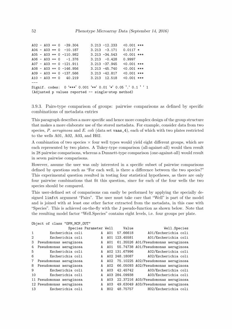
52 Phenotype Microarray Data (September 14, 2016)
A02 - A03 == 0 -39.304 3.213 -12.233 <0.001 ***
A04 - A03 == 0 -10.187 3.213 -3.171 0.0117 *
A05 - A03 == 0 -110.982 3.213 -34.543 <0.001 ***
A06 - A03 == 0 -1.376 3.213 -0.428 0.9997
A07 - A03 == 0 -121.911 3.213 -37.945 <0.001 ***
A08 - A03 == 0 -146.956 3.213 -45.740 <0.001 ***
A09 - A03 == 0 -137.566 3.213 -42.817 <0.001 ***
A10 - A03 == 0 40.219 3.213 12.518 <0.001 ***
---
Signif. codes: 0 ✬***✬ 0.001 ✬**✬ 0.01 ✬*✬ 0.05 ✬.✬ 0.1 ✬ ✬ 1
(Adjusted p values reported -- single-step method)
3.9.3. Pairs-type comparison of groups: pairwise comparisons as defined by specificcombinations of metadata entries
This paragraph describes a more specific and hence more complex design of the group structurethat makes a more elaborate use of the stored metadata. For example, consider data from twospecies, P. aeruginosa and E. coli (data set vaas_4), each of which with two plates restrictedto the wells A01, A02, A03, and H02.
A combination of two species × four well types would yield eight different groups, which areeach represented by two plates. A Tukey-type comparison (all-against-all) would then resultin 28 pairwise comparisons, whereas a Dunnett-type comparison (one-against-all) would resultin seven pairwise comparisons.
However, assume the user was only interested in a specific subset of pairwise comparisonsdefined by questions such as “For each well, is there a difference between the two species?”This experimental question resulted in testing four statistical hypotheses, as there are onlyfour pairwise combinations that fit this question, since for each of the four wells the twospecies should be compared.
This user-defined set of comparisons can easily be performed by applying the specially de-signed linfct argument “Pairs”. The user must take care that “Well” is part of the modeland is joined with at least one other factor extracted from the metadata, in this case with“Species”. This is achieved on-the-fly with the J pseudo-function as shown below. Note thatthe resulting model factor “Well.Species” contains eight levels, i.e. four groups per plate.
Object of class "OPM_MCP_OUT"
Species Parameter Well Value Well.Species
1 Escherichia coli A A01 57.66618 A01/Escherichia coli
2 Escherichia coli A A01 123.45581 A01/Escherichia coli
3 Pseudomonas aeruginosa A A01 61.35526 A01/Pseudomonas aeruginosa
4 Pseudomonas aeruginosa A A01 55.74738 A01/Pseudomonas aeruginosa
5 Escherichia coli A A02 131.67996 A02/Escherichia coli
6 Escherichia coli A A02 248.18087 A02/Escherichia coli
7 Pseudomonas aeruginosa A A02 75.10225 A02/Pseudomonas aeruginosa
8 Pseudomonas aeruginosa A A02 66.05093 A02/Pseudomonas aeruginosa
9 Escherichia coli A A03 42.45742 A03/Escherichia coli
10 Escherichia coli A A03 284.09938 A03/Escherichia coli
11 Pseudomonas aeruginosa A A03 22.37216 A03/Pseudomonas aeruginosa
12 Pseudomonas aeruginosa A A03 49.63049 A03/Pseudomonas aeruginosa
13 Escherichia coli A H02 48.75757 H02/Escherichia coli

M. Goker, B. Hofner, M.d.C. Montero Calasanz, J. Sikorski, L.A.I. Vaas 53
14 Escherichia coli A H02 63.62915 H02/Escherichia coli
15 Pseudomonas aeruginosa A H02 294.68878 H02/Pseudomonas aeruginosa
16 Pseudomonas aeruginosa A H02 312.19430 H02/Pseudomonas aeruginosa
As explained above, the name of the linfct value indicates the type of contrast used for thetesting procedure. Unless explicitly specified, “Pairs” selects the first subcomponent from thepreviously selected (joined) model component for the comparisons. Explicitly setting linfct
= c(Pairs.Well = 1) ensures that for all levels present in the first (joined) component ofthe model, i.e, Well-wise, all pairwise comparisons are performed between the defined groups(here: the two species P. aeruginosa and E. coli).
The result of this analysis is shown below.
R> y <- opm_mcp(vaas_4[, , c(1:3, 86)], model = ~ J(Well, Species),
m.type = "aov", linfct = c(Pairs.Well = 1), full = FALSE)
Simultaneous Tests for General Linear Hypotheses
Multiple Comparisons of Means: User-defined Contrasts
Linear Hypotheses:
Estimate Std. Error t value
❵A01/Pseudomonas aeruginosa❵ - ❵A01/Escherichia coli❵ == 0 -32.01 69.68 -0.459
❵A02/Pseudomonas aeruginosa❵ - ❵A02/Escherichia coli❵ == 0 -119.35 69.68 -1.713
❵A03/Pseudomonas aeruginosa❵ - ❵A03/Escherichia coli❵ == 0 -127.28 69.68 -1.827
❵H02/Pseudomonas aeruginosa❵ - ❵H02/Escherichia coli❵ == 0 247.25 69.68 3.549
Pr(>|t|)
❵A01/Pseudomonas aeruginosa❵ - ❵A01/Escherichia coli❵ == 0 0.9816
❵A02/Pseudomonas aeruginosa❵ - ❵A02/Escherichia coli❵ == 0 0.3753
❵A03/Pseudomonas aeruginosa❵ - ❵A03/Escherichia coli❵ == 0 0.3240
❵H02/Pseudomonas aeruginosa❵ - ❵H02/Escherichia coli❵ == 0 0.0271 *
---
Signif. codes: 0 ✬***✬ 0.001 ✬**✬ 0.01 ✬*✬ 0.05 ✬.✬ 0.1 ✬ ✬ 1
(Adjusted p values reported -- single-step method)
Particularly if models are more complex, e.g., if more than two metadata entries would bejoined by the J function, it is highly recommended to explicitly set the names of the metadataentries for which the pairwise comparisons should be performed by appending it directly tothe Pairs argument. For instance, in our example the metadata name Species is directlyaddressed with linfct = c(Pairs.Species = 1), which results in the pairwise all-against-all comparisons of the selected four wells within each of the two species Escherichia coli andPseudomonas aeruginosa.
R> y <- opm_mcp(vaas_4[, , c(1:3, 86)], model = ~ J(Well, Species), m.type = "aov",
linfct = c(Pairs.Species = 1), full = FALSE)
R> mcp.summary <- summary(y)
R> mcp.summary$model$call <- NULL # avoid some unnecessary output
R> mcp.summary

54 Phenotype Microarray Data (September 14, 2016)
Simultaneous Tests for General Linear Hypotheses
Multiple Comparisons of Means: User-defined Contrasts
Linear Hypotheses:
Estimate Std. Error
❵A02/Escherichia coli❵ - ❵A01/Escherichia coli❵ == 0 99.37 69.68
❵A03/Escherichia coli❵ - ❵A01/Escherichia coli❵ == 0 72.72 69.68
❵H02/Escherichia coli❵ - ❵A01/Escherichia coli❵ == 0 -34.37 69.68
❵A03/Escherichia coli❵ - ❵A02/Escherichia coli❵ == 0 -26.65 69.68
❵H02/Escherichia coli❵ - ❵A02/Escherichia coli❵ == 0 -133.74 69.68
❵H02/Escherichia coli❵ - ❵A03/Escherichia coli❵ == 0 -107.09 69.68
❵A02/Pseudomonas aeruginosa❵ - ❵A01/Pseudomonas aeruginosa❵ == 0 12.03 69.68
❵A03/Pseudomonas aeruginosa❵ - ❵A01/Pseudomonas aeruginosa❵ == 0 -22.55 69.68
❵H02/Pseudomonas aeruginosa❵ - ❵A01/Pseudomonas aeruginosa❵ == 0 244.89 69.68
❵A03/Pseudomonas aeruginosa❵ - ❵A02/Pseudomonas aeruginosa❵ == 0 -34.58 69.68
❵H02/Pseudomonas aeruginosa❵ - ❵A02/Pseudomonas aeruginosa❵ == 0 232.86 69.68
❵H02/Pseudomonas aeruginosa❵ - ❵A03/Pseudomonas aeruginosa❵ == 0 267.44 69.68
t value Pr(>|t|)
❵A02/Escherichia coli❵ - ❵A01/Escherichia coli❵ == 0 1.426 0.7298
❵A03/Escherichia coli❵ - ❵A01/Escherichia coli❵ == 0 1.044 0.9070
❵H02/Escherichia coli❵ - ❵A01/Escherichia coli❵ == 0 -0.493 0.9974
❵A03/Escherichia coli❵ - ❵A02/Escherichia coli❵ == 0 -0.383 0.9994
❵H02/Escherichia coli❵ - ❵A02/Escherichia coli❵ == 0 -1.919 0.4603
❵H02/Escherichia coli❵ - ❵A03/Escherichia coli❵ == 0 -1.537 0.6685
❵A02/Pseudomonas aeruginosa❵ - ❵A01/Pseudomonas aeruginosa❵ == 0 0.173 1.0000
❵A03/Pseudomonas aeruginosa❵ - ❵A01/Pseudomonas aeruginosa❵ == 0 -0.324 0.9998
❵H02/Pseudomonas aeruginosa❵ - ❵A01/Pseudomonas aeruginosa❵ == 0 3.515 0.0580 .
❵A03/Pseudomonas aeruginosa❵ - ❵A02/Pseudomonas aeruginosa❵ == 0 -0.496 0.9974
❵H02/Pseudomonas aeruginosa❵ - ❵A02/Pseudomonas aeruginosa❵ == 0 3.342 0.0735 .
❵H02/Pseudomonas aeruginosa❵ - ❵A03/Pseudomonas aeruginosa❵ == 0 3.838 0.0376 *
---
Signif. codes: 0 ✬***✬ 0.001 ✬**✬ 0.01 ✬*✬ 0.05 ✬.✬ 0.1 ✬ ✬ 1
(Adjusted p values reported -- single-step method)
This yields 2× 6 = 12 pairwise comparisons (two species, and six all-against-all comparisonsbetween four wells) for which the adjustment of multiplicity has been undertaken.
When dealing with more complex models keep in mind that a numeric linfct argument canrefer to the position of any variable, or set of variables obtained by joining, within model.
3.9.4. User-defined comparisons of interest
For performing even more specific comparisons of interest, the user would directly provide acontrast matrix. Such a contrast for multiple comparison procedures is defined as a linearcombination of two or more factor-level means whose coefficients add up to 0 (Hochberg andTamhane 1987). To demonstrate the principle of a contrast matrix, we here perform anall-against-all comparison (a “Tukey”-type contrast) of four groups using a toy example.
R> library("multcomp") # now needed
R> n <- c(10, 20, 30, 40)
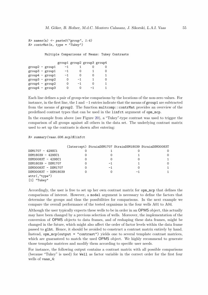
M. Goker, B. Hofner, M.d.C. Montero Calasanz, J. Sikorski, L.A.I. Vaas 55
R> names(n) <- paste0("group", 1:4)
R> contrMat(n, type = "Tukey")
Multiple Comparisons of Means: Tukey Contrasts
group1 group2 group3 group4
group2 - group1 -1 1 0 0
group3 - group1 -1 0 1 0
group4 - group1 -1 0 0 1
group3 - group2 0 -1 1 0
group4 - group2 0 -1 0 1
group4 - group3 0 0 -1 1
Each line defines a pair of group-wise comparisons by the locations of the non-zero values. Forinstance, in the first line, the 1 and−1 entries indicate that the means of group1 are subtractedfrom the means of group2. The function multcomp::contrMat provides an overview of thepredefined contrast types that can be used in the linfct argument of opm_mcp.
In the example from above (see Figure 20), a “Tukey”-type contrast was used to trigger thecomparison of all groups against all others in the data set. The underlying contrast matrixused to set up the contrasts is shown after entering:
R> summary(vaas.G06.mcp)$linfct
(Intercept) StrainDSM1707 StrainDSM18039 StrainDSM30083T
DSM1707 - 429SC1 0 1 0 0
DSM18039 - 429SC1 0 0 1 0
DSM30083T - 429SC1 0 0 0 1
DSM18039 - DSM1707 0 -1 1 0
DSM30083T - DSM1707 0 -1 0 1
DSM30083T - DSM18039 0 0 -1 1
attr(,"type")
[1] "Tukey"
Accordingly, the user is free to set up her own contrast matrix for opm_mcp that defines thecomparisons of interest. However, a model argument is necessary to define the factors thatdetermine the groups and thus the possibilities for comparisons. In the next example wecompare the overall performance of the tested organisms in the four wells A01 to A04.
Although the user typically expects these wells to be in order in an OPMS object, this actuallymay have been changed by a previous selection of wells. Moreover, the implementation of theconversion of OPMS objects to data frames, and of reshaping these data frames, might bechanged in the future, which might also affect the order of factor levels within the data framepassed to glht. Hence, it should be avoided to construct a contrast matrix entirely by hand.Instead, opm_mcp(output = "contrast") yields one to several template contrast matrices,which are guaranteed to match the used OPMS object. We highly recommend to generatethose template matrices and modify them according to specific user needs.
For instance, the following output contains a contrast matrix with all possible comparisons(because “Tukey” is used) for Well as factor variable in the correct order for the first fourwells of vaas_4:

56 Phenotype Microarray Data (September 14, 2016)
−300 −200 −100 0 100 200
A04 − A03
A04 − A01
A03 − A01
A02 − A01 (
(
(
(
)
)
)
)
●
●
●
●
95% family−wise confidence level
Figure 21: Point estimates and 95% confidence intervals in a manually defined comparisonof group means for a specifically selected set of wells (A01 to A04) from the vaas_4 exemplarobject. The picture was obtained by running opm_mcp and then plotting the resulting object.Compare this with Figure 20 regarding the axis annotation.
R> contr <- opm_mcp(vaas_4[, , 1:4], model = ~ Well, linfct = c(Tukey = 1),
output = "contrast", full = FALSE)
R> contr
The contr object is a named list of contrast matrices with one matrix per selected factor. Anaccording call of the opm_mcp function including the selecting of some comparisons of interestis:
R> vaas4.mcp <- opm_mcp(vaas_4[, , 1:4], model = ~ Well, m.type = "lm",
linfct = contr$Well[c(1:3, 6), ], full = FALSE)
Since output = "contrast" does not work in this situation, the definition of the contrastmatrix is controlled with:
R> summary(vaas4.mcp)$linfct
A01 A02 A03 A04
A02 - A01 -1 1 0 0
A03 - A01 -1 0 1 0
A04 - A01 -1 0 0 1
A04 - A03 0 0 -1 1
As mentioned above, the outcome is visualised using the plot method for glht objects (seeFigure 21).
Note that the model argument defines the group means available for comparison. In thefollowing example “Species” contains only two levels (“Pseudomonas aeruginosa” and “Es-cherichia coli”). Thus only one comparison is possible, irrespective of the requested contrasttype.
R> vaas4.mcp <- opm_mcp(vaas_4, model = ~ Species, m.type = "lm",
linfct = mcp(Species = "Dunnett"))
Finally, in addition to the multiple comparison of single group means as described above, it ispossible to compare averages from several subgroups with a single other subgroup or averagesfrom several other subgroups. For instance, the user might be interested in comparing thedata shown in Figure 22 at the level of groups that contained distinct data sets as subgroups.

M. Goker, B. Hofner, M.d.C. Montero Calasanz, J. Sikorski, L.A.I. Vaas 57
−50 −40 −30 −20 −10 0 10
DSM30083T/Second replicate − 429SC1/First replicate
DSM30083T/First replicate − 429SC1/First replicate
DSM18039/Time series − 429SC1/First replicate
DSM18039/Second replicate − 429SC1/First replicate
DSM18039/First replicate − 429SC1/First replicate
DSM1707/Second replicate − 429SC1/First replicate
DSM1707/First replicate − 429SC1/First replicate
429SC1/Second replicate − 429SC1/First replicate (
(
(
(
(
(
(
(
)
)
)
)
)
)
)
)
●
●
●
●
●
●
●
●
95% family−wise confidence level
Figure 22: Point estimates and 95% confidence intervals in a Dunnett-type comparisonof group means for a cell-means model for the vaas.G06 exemplar object. In analogy toFigure 21, the picture was obtained by running opm_mcp and then the plotting function forthe resulting object. Compare with Figure 20 for the axis annotation.
R> vaas.G06 <- vaas_et_al[, , "G06"]
R> vaas.G06.mcp <- opm_mcp(vaas.G06, model = ~ J(Strain, Experiment),
linfct = c(Dunnett = 1))
The result is shown in Figure 22, visualised using plot as described above.
Note that for defining a contrast matrix the levels of the model-defining factor need to matchthe columns of the contrast matrix, in order. For this reason, it is advantageous to workwith a template contrast matrix generated with opm_mcp from the object under study and toinvestigate the positioning of its column names prior to any modification:
R> contr <- opm_mcp(vaas.G06, model = ~ J(Strain, Experiment),
linfct = c(Dunnett = 1), output = "contrast")$Strain.Experiment
R> colnames(contr)
The user is then free to choose other values than just 0 and 1 for the coefficients, providedthat each contrast sums up to zero. In the example below, the contrast matrix is reduced tothree contrasts of interest, in which the values 0, −1/4 , 1/4, and 1 are used. At this pointthe reader might already have noted that the “First replicate” entries are in columns 1, 3,5 and 8, whereas the “Second replicate” entries are in columns 2, 4, 6 and 9 and the “Timeseries” entries are in column 7 of the object contr. This information is sufficient to define acorrect contrast matrix for the following three contrasts of interest:
R> contr <- contr[1:3, ] # keeps the column names
R> rownames(contr) <- c(
"First repl. - Second repl.",
"First repl. - Time series",
"DSM 1707 #1 - Second repl."
)
R> contr[1, ] <- c(1 / 4, -1 / 4, 1 / 4, -1 / 4, 1 / 4, -1 / 4, 0, 1 / 4, -1 / 4)
R> contr[2, ] <- c(1 / 4, 0, 1 / 4, 0, 1 / 4, 0, -1, 1 / 4, 0)

58 Phenotype Microarray Data (September 14, 2016)
−10 −5 0 5
DSM 1707 #1 − Second repl.
First repl. − Time series
First repl. − Second repl. (
(
(
)
)
)
●
●
●
95% family−wise confidence level
Figure 23: Point estimates and 95% confidence intervals in a user defined comparison ofgroup means for a cell-means model for the vaas.G06 exemplar object. Like Figure 21, thepicture was obtained by first applying opm_mcp and then the plotting function for the resultingobject. Compare with Figure 20 for the axis annotation.
R> contr[3, ] <- c(0, -1 / 4, 1, -1 / 4, 0, -1 / 4, 0, 0, -1 / 4)
R> contr
R> vaas6.mcp <- opm_mcp(vaas.G06, model = ~ J(Strain, Experiment), m.type = "lm",
linfct = mcp(Strain.Experiment = contr))
The resulting visualisation of this entirely user-defined contrast matrix is shown in Figure 23.
3.9.5. Troubleshooting
Note that you need data sets which actually provide group structures for comparisons. Theseare, e.g., strains measured on the same plate type in several repetitions, or one strain treateddifferentially with each treatment measured in several repetitions. It is also possible, of course,to compare the wells with each other if the plates are comparable. But with a single valueper group opm_mcp will inevitably raise an error.
3.10. Discretisation
After calculating curve parameters, data can be discretised and optionally also exported foranalysis with external phylogeny software or for inclusion into a scientific manuscript as textor table. In the opm manual and help pages, the functions for either task are contained inthe families “discretisation-functions”, “phylogeny-functions” and partially also in “naming-functions”, with according cross-references. Much like do_aggr for aggregation, do_disc
should be preferred for discretisation. By default it works on the A parameter (see Figure 6)but this can be modified.
3.10.1. Discretisation and phylogenetic data export
Restricting the vaas_et_al example data set to the two biological replicates yields an orthog-onal data set with 2 × 10 replicates for each of the four strains, for which we can calculatediscretised parameters:
R> vaas.repl <- subset(vaas_et_al,
query = list(Experiment = c("First replicate", "Second replicate")))
R> vaas.repl <- do_disc(vaas.repl)

M. Goker, B. Hofner, M.d.C. Montero Calasanz, J. Sikorski, L.A.I. Vaas 59
Note that the resulting object is an OPMS object with OPMD objects as elements. Suchobjects contain discretised values, available via discretised, as well as the discretisation set-tings used, available via disc_settings. This works much like aggregated and aggr_settingsexplained above. disc_settings also yields the computed discretisation cutoffs. The subsetfunction has a positive argument that allows one to create a subset containing only the wellsthat were positive in at least one plate or in all plates, as well as a corresponding negative
argument. The effect of either could be modified with subset(invert = TRUE). For ex-ample, the command xy_plot(subset(vaas_4, positive = "all"), neg.ctrl = NULL)
would plot only those wells in which all curves have been classified by k-means partition-ing to yield a positive reaction. Look up opm::subset in the manual for further information.
3.10.2. Discretisation and export of text
The listing methods of the OPMD and OPMD classes create textual descriptions of thediscretisation results suitable for the direct inclusion in scientific manuscripts.
R> listing(vaas.repl, as.groups = NULL)
R> listing(vaas.repl, as.groups = list("Species"))
As usual, the results can be grouped according to specified metadata entries using theas.groups argument. If this yields ambiguities (such as a negative reaction of the samewell on one plate and a positive reaction on another plate), the result is accordingly renamed.The cutoff argument can be used to define filters, keeping only those values that occur in aspecified minimum proportion of wells, as described in the opm::listing entry in the manual.
The listing function returns a character vector or matrix with the S3 class OPMD listing orOPMS listing, allowing for a special phylo_data function that further formats these objects.Accordingly, the following code snippets:
R> phylo_data(listing(vaas.repl, as.groups = NULL))
R> phylo_data(listing(vaas.repl, as.groups = list("Species")))
yield character scalars better suitable for exporting into text files using write. It is alsopossible to generate HTML output, yielding formatted text. Try
R> phylo_data(listing(vaas.repl, as.groups = NULL, html = TRUE))
R> phylo_data(listing(vaas.repl, as.groups = list("Species"), html = TRUE))
and note that the phylo_data function has a html.args argument. Textual HTML outputsupports most of the formatting instructions for the output of HTML tables described below(see 3.10.3). Note particularly how formatting via a Cascading Style Sheets (CSS) file works,as described in Section 3.10.3.
The default settings of do_disc imply exact k-means partitioning into three groups (“neg-ative”, “ambiguous” and “positive”), treating all contained plates together, and using themaximum-height parameter for discretisation. Let A1 and A2 be the A parameters from twocurves C1 and C2, respectively, and let us assume that A1 ≥ A2 holds. The algorithm thenguarantees that if C2 is judged as positive reaction then C1 is also judged as positive; if C2 isweak then C1 is not negative; if C1 is negative then C2 is negative; and if C1 is weak then C2 is

60 Phenotype Microarray Data (September 14, 2016)
not positive. In this sense, the results will be consistent, but there are not many other thingsthe algorithm guarantees. Note particularly that always three clusters result by default (onecan omit the middle cluster, i.e. the “weak” reactions), irrespective of the input data. This isusually without difficulty if the data contain both really negative and really positive reactions,but data that in reality are negative throughout, or uniformly positive, would neverthelessbe split into three (or two) clusters. That is, additionally checking the curve heights andparticularly the “cutoffs” entry obtained via disc_settings should initially be mandatory.
It is also possible to make the reactions uniform within metadata-defined groups. This wouldbe specified with the unify argument and would deliberately deviate from the kind of consis-tency described above. The unification approach replaces the primary discretisation resultswith the most frequent value within the respective combination of group and well if this valueis present in a given proportion of the original values and with NA otherwise. The accord-ing cutoff is set using opm_opt(min.mode = ...) or directly. Thus there are two distinctmeanings of “ambiguous” reactions, as ambiguity either results from the clustering of the pa-rameters, or by clustering results that deviate between distinct experimental replications. Itis unnecessary and perhaps not preferable to use both approaches together, i.e. to clusterinto three groups only and then also unify. Note that listing and phylo_data would usethe same unification approach, if requested.
The manual of do_disc describes the other discretisation approaches available in opm, such asusing best_cutoff instead of k-means partitioning, and using subsets of the plates, specifiedusing stored metainformation.
3.10.3. Discretisation and export of tables
The HTML created by opm deliberately contains no formatting instructions. Rather, it ispossible (and recommended) to link it to a CSS file or embed such a file. CSS is a style-sheetlanguage used for defining the formatting of a document written in a markup language suchas HTML.
As the generated HTML is richly annotated with “class” attributes, which not only provideinformation on the structure of the file but also on the depicted data, very specific formattingcan be obtained just by modifying one to several associated CSS files. For the followingexample, we set the default CSS file to be linked from the generated HTML to the first CSSfile that comes with opm.
R> opm_opt(css.file = opm_files("css")[[1]])
One could now easily create an HTML table from the discretised data and write it to a file:
R> vaas.html <- phylo_data(vaas.repl, format = "html",
as.labels = list("Species", "Strain"), outfile = "vaas.html")
A practical problem is that the resulting HTML file is linked to its CSS file with a fixedpath. The formatting would thus get lost once the HTML file was copied to another system,without a warning. Hence, users might want to copy the predefined CSS file to the workingdirectory and set it as default, or embed the CSS file directly into HTML:
R> vaas.html <- phylo_data(vaas.repl, format = "html",
html.args = html_args(embed.css = TRUE),

M. Goker, B. Hofner, M.d.C. Montero Calasanz, J. Sikorski, L.A.I. Vaas 61
as.labels = list("Species", "Strain"), outfile = "vaas.html")
R> ## the alternative: copying the file into the working directory
R> # file.copy(opm_files("css")[[1]], "opm_styles.css", overwrite = TRUE)
R> # opm_opt(css.file = "opm_styles.css")
The generated HTML would subsequently be linked to this file, and the two files could bedistributed together, or the CSS from the file would directly be embedded in the HTML.The same mechanism works for text generation using listing (see 3.10.2). In addition tothe default CSS file, a complete list of the settings that can be modified with this function isavailable in the opm_opt entry of the manual.
Users who want to define their own CSS files can start with modifying the file shipped withopm. Microsoft Windows users should consider that the path to the linked file must beprovided in UNIX style, as obtained, e.g., using normalizePath(x, winslash = "/") if xis the path to the file. This is according to World Wide Web (WWW) standards and notdetermined by opm.
By default columns with measurement repetitions as specified using as.labels are joinedtogether. The delete argument specifies how to reduce the table: either not at all or keep-ing only the variable, parsimony-informative or non-ambiguous characters. The legend ofthe table is as used in taxonomic journals such as the International Journal of Systematicand Evolutionary Microbiology (http://ijs.sgmjournals.org/) but could also be adapted.Users can modify the headline, add sections before the table legend, or before or after thetable. The title and the “meta” entries of the resulting HTML can also be modified. Thephylo_data methods have an auxiliary function, html_args, which assists in putting to-gether the arguments that determine the shape and content of the HTML output. Look upthe manual for further information on html_args.
3.10.4. Fine-tuning the discretisation
One can also conduct discretisation step-by-step by using the functions best_cutoff ordiscrete after extracting matrices from the OPMS object. This is more flexible (and hasadditional discretisation approaches, e.g. the creation of multiple-state characters) but is alsomore tedious than using do_disc.
R> vaas.repl <- subset(vaas_et_al,
query = list(Experiment = c("First replicate", "Second replicate")))
R> vaas.repl <- extract(vaas.repl,
as.labels = list("Species", "Strain", "Experiment", "Plate number"))
The A parameter (see Figure 6) can be discretised into (per default) 32 states using thetheoretical range of 0 to 400 OmniLog➤ units (see Section 2.10):
R> vaas.repl.disc <- discrete(vaas.repl, range = c(0, 400))
This yields (at most) 32 distinct character states corresponding to the 32 equal-width inter-vals within 0 and 400. Exporting the data in extended PHYLIP format readable by RAxML
(Stamatakis et al. 2005) works as follows:
R> phylo_data(vaas.repl.disc, outfile = "example_replicates.epf")

62 Phenotype Microarray Data (September 14, 2016)
The other supported formats are PHYLIP, NEXUS and TNT (Goloboff et al. 2008). Fordiscretising the data not in equally spaced intervals but into binary characters includingmissing data, or ternary characters with a third, intermediary state between ”negative” and”positive” the gap mode of discrete can be used:
R> vaas.repl.disc <- discrete(vaas.repl, range = c(120.2, 236.6), gap = TRUE)
Here the range argument does not provides the overall boundaries of the data as before (atleast as large as the real range), but the boundaries of a zone within the real range of thedata corresponding to an area of ambiguous affiliation. That is, values below 120.2 are codedas “0”, those above 236.6 as “1”, and those in between as “?”. The values used above weredetermined by k-means partitioning of the A values from the vaas_et_al data set (Vaas et al.2012); there is currently no conclusive evidence that they can generally be applied. The lastcommand results in the treatment of values within the given range as “missing data” (NA inR, “?” if exported). To treat them as a third, intermediary character state, set middle.na toFALSE:
R> vaas.repl.disc <- discrete(vaas.repl, range = c(120.2, 236.6),
gap = TRUE, middle.na = FALSE)
The three resulting states, coded as “0”, “1” and “2” (in contrast to “0”, “?” and “1” above)have to be interpreted as “negative”, “weak” and “positive”. Exporting the data in one of thesupported phylogeny formats works as described above. If the do_disc function describedabove calls discrete, then only in gap mode and with middle.na set to TRUE, yielding avector or logical matrix.
4. Discussion and conclusion
The high-dimensional sets of longitudinal data collected by the OmniLog➤ PM system callfor fast and easily applicable (and extensible) data organisation and analysis facilities. Thehere presented opm package for the free statistical software R (R Development Core Team2011) features not only the calculation of aggregated values (curve parameters) includingtheir (bootstrapped) confidence intervals, but also provides a rather complete infrastructurefor the management of raw kinetic values and curve parameters together with any kind ofmeta-information of relevance for the user (Vaas et al. 2012, 2013a).
The spline estimation and parameter calculation in the data-aggregation step of has beenoptimised for the analysis of PM data. One main issue in the spline-fitting procedure is theselection of suitable smoothing parameters. The methods included in opm provide not only thebasic framework (Vaas et al. 2012) based on methods from the grofit package (Kahm et al.2010), but also specifically adapted applications of smooth.spline and the mgcv package(Wood 2003; Eilers and Marx 1996)
The analysis toolbox of the package includes the implementation of a fully automated esti-mation of whether respiration kinetics should be classified as either a “positive” or “negative”(absent) physiological reaction. This dichotomisation is apparently of high interest to manyusers of the OmniLog➤ PM system but would apparently be extremely biased as long as

M. Goker, B. Hofner, M.d.C. Montero Calasanz, J. Sikorski, L.A.I. Vaas 63
thresholds are chosen ad hoc and by eye. Users should nevertheless be aware that loss ofinformation is inherent to discretising continuous data.
The opm package enables the user to produce highly informative and specialised graphicaloutputs from both the raw kinetic data as well as the curve-parameter estimates. Moreover,the package provides simultaneous multiple comparisons of group means (Hothorn et al. 2008;Bretz et al. 2010; Hsu 1996) with an interface specifically adapted to the typical PM dataobjects. In combination with the functionality for annotating the data with meta-informationand then selecting subsets of the data, straightforward analyses regarding specific analyticalquestions can be performed without the need to invoke other R packages.
But since the design of the opm objects is not intended to be limited to specific analysisframeworks, the opm package works as a data containment providing well organised andcomprehensive PM data for further, more specialised analyses using methods from differentR packages or other third-party software tools. Particularly the generation of S4 objectsfeaturing a rich set of methods as containers for either single or multiple OmniLog➤ PMplates enables not only the transfer of raw kinetic data into R but also eases their furtherprocessing. The complex data bundles can also be exported in YAML format, which is ahuman-readable data serialisation format that can be read by most common programminglanguages and facilitates fast and easy data exchange between laboratories. If a proper YAMLparser was unavailable, its subset JSON could also be used. The interaction between opm
and databases is partially also based on these formats; see Section 2.12. The package can alsogenerate CSV output files, but due to the limitation of this format these files cannot be readback into opm in a meaningful way (but into R).
Power and limitations regarding usage of substrate information and their implementation fordata arrangement and hypothesis testing (Hofner, Boccuto, and Goker 2015) are discussed indetail in the vignette “Working with substrate information in opm”.
These features render the opm package the first comprehensive toolbox for the managementand a broad range of analyses of OmniLog➤ PM data. Its usage requires some familiaritywith R, but is otherwise intuitive and straightforward also for biologists who are not used tocommand-line based software. To summarise, we are convinced that the opm package alreadyenables the users to analyse OmniLog➤ PM data in rather unlimited exploratory directions(Vaas et al. 2012, 2013a).
5. Acknowledgements
The help of Nora Buddruhs (DSMZ) and Anne Fiebig (DSMZ), who contributed a lot to thestored substrate information and to examples in earlier versions of this tutorial, is gratefullyacknowledged. We owe very much to Hans-Peter Klenk (DSMZ), who brought the Om-niLog➤ instrument to the DSMZ and supported this project in numerous ways. We thankBarry Bochner (BIOLOG Inc.), John Kirkish (BIOLOG Inc.), Andre Chouankam (BIOLOGInc.), Jan Meier-Kolthoff (DSMZ), Pia Wust (DSMZ), Stefan Ehrentraut (DSMZ) and JornPetersen (DSMZ) for helpful advice, as well as Victoria Michael (DSMZ) for technical support.We are also grateful to the maintainers of R-Forge for providing the on-line resources used bythis project, and to the maintainers of the R on which opm depends for making their packagesfreely available. This work was supported by the Deutsche Forschungsgemeinschaft (DFG)Sonderforschungsbereich (SFB)/Transregio (TRR) 51 and by the Microme project within the

64 Phenotype Microarray Data (September 14, 2016)
Framework 7 programme of the European Commission, which is gratefully acknowledged.Johannes Sikorski gratefully acknowledges his support by DFG grant SI 1352/1-2.
References
Berger S, Stamatakis A (2010). “Accuracy of Morphology-Based Phylogenetic Fossil Place-ment under Maximum Likelihood.” In 8th ACS/IEEE International Conference on Com-puter Systems and Applications (AICCSA-10). ACS/IEEE, Hammamet, Tunisia.
BiOLOG Inc (2009). Converter, File Management Software, Parametric Software, PhenotypeMicroArray, User Guide, Part 90333. Biolog Inc., Hayward CA.
Bochner B (2009). “Global Phenotypic Characterization of Bacteria.” FEMS MicrobiologicalReviews, 33, 191–205. doi:10.1111/j.1574-6976.2008.00149.x.
Bochner B, Gadzinski P, Panomitros E (2001). “Phenotype MicroArrays for High ThroughputPhenotypic Testing and Assay of Gene Function.” Genome Research, 11, 1246–1255. doi:10.1101/gr.186501.
Bochner B, Savageau M (1977). “Generalized Indicator Plate for Genetic, Metabolic, andTaxonomic Studies with Microorganisms.” Applied and Environmental Microbiology, 33,434–444.
Bochner BR, Siri M, Huang RH, Noble S, Lei XH, Clemons PA, Wagner BK (2011). “Assayof the Multiple Energy-Producing Pathways of Mammalian Cells.” PLoS ONE, 6, e18147.doi:10.1371/journal.pone.0018147.
Bretz F, Hothorn T, Westfall P (2010). Multiple Comparisons Using R. CRC Press, BocaRaton.
Brisbin I, Collins C, White G, McCallum D (1987). “A New Paradigm for the Analysis andInterpretation of Growth Data: The Shape of Things to Come.” The Auk, 104, 552–553.
Broadbent J, Larsen R, Deibel V, Steele J (2010). “Physiological and Transcriptional Responseof Lactobacillus casei ATCC 334 to Acid Stress.” Journal of Bacteriology, 192, 2445–2458.doi:10.1128/JB.01618-09.
Caspi R, Billington R, Ferrer L, Foerster H, Fulcher CA, Keseler IM, Kothari A, Krumme-nacker M, Latendresse M, Mueller LA, Ong Q, Paley S, Subhraveti P, Weaver DS, KarpPD (2016). “The MetaCyc database of metabolic pathways and enzymes and the Bio-Cyc collection of pathway/genome databases.” Nucleic Acids Research, 44, D471–D480.doi:10.1093/nar/gkv1164.
Chaiboonchoe A, Dohai BS, Cai H, Nelson DR, Jijakli K, Salehi-Ashtiani K (2014). “Microal-gal Metabolic Network Model Refinement through High Throughput Functional MetabolicProfiling.” Frontiers in Bioengineering and Biotechnology, 2. ISSN 2296-4185. doi:
10.3389/fbioe.2014.00068.
Chambers J (1998). Programming with Data. Statistics and Computing. Springer-Verlag,New York.

M. Goker, B. Hofner, M.d.C. Montero Calasanz, J. Sikorski, L.A.I. Vaas 65
Champely S (2012). pwr: Basic functions for power analysis. R package version 1.1.1, URLhttp://CRAN.R-project.org/package=pwr.
Chheng T (2013). RMongo: MongoDB Client for R. R package version 0.0.25, URL http:
//CRAN.R-project.org/package=RMongo.
Conway J, Eddelbuettel D, Nishiyama T, Prayaga SK, Tiffin N (2013). RPostgreSQL: Rinterface to the PostgreSQL database system. R package version 0.4, URL http://CRAN.
R-project.org/package=RPostgreSQL.
Dilba G, Bretz F, Guiard V (2006). “Simultaneous confidence sets and confidence intervalsfor multiple ratios.” Journal of Statistical Planning and Inference, 136, 2640–2658. doi:
10.1016/j.jspi.2004.11.009.
Djira GD, Hasler M, Gerhard D, Schaarschmidt F (2012). mratios: Inferences for ratiosof coefficients in the general linear model. R package version 1.3.17, URL http://CRAN.
R-project.org/package=mratios.
Dougherty J, Kohavi R, Sahami M (1995). “Supervised and Unsupervised Discretization ofContinuous Features.” In A Prieditis, S Russell (eds.), Machine Learning: Proceedings ofthe fifth international conference.
Efron B (1979). “Bootstrap Methods: Another Look at the Jackknife.” The Annals of Statis-tics, 7, 1–26.
Eilers P, Marx B (1996). “Flexible Smoothing with B-splines and Penalties.” StatisticalSciences, 11, 89–121.
Eng J (2003). “Sample size estimation: How many individuals should be studied?” Radiology,227, 309–313. doi:10.1148/radiol.2272012051.
Farris J (1970). “Methods for Computing Wagner Trees.” Systematic Zoology, 19, 83–92.
Felsenstein J (2004). Inferring Phylogenies. Sinauer Associates, Inc., Sunderland, MA.
Fitch W (1971). “Towards Defining the Course of Evolution: Minimal Change for a SpecifiedTree Topology.” Systematic Zoology, 20, 406–416.
Goloboff P, Farris J, Nixon K (2008). “TNT, a Free Program for Phylogenetic Analysis.”Cladistics, 24, 774–786. doi:10.1111/j.1096-0031.2008.00217.x.
Hasler M (2012a). “Multiple comparisons to both a negative and a positive control.” Phar-maceutical Statistics, 11, 74–81. doi:10.1002/pst.503.
Hasler M (2012b). SimComp: Simultaneous Comparisons for Multiple Endpoints. R packageversion 1.7.0, URL http://CRAN.R-project.org/package=SimComp.
Hochberg A, Tamhane Y (1987). Multiple Comparison Procedures. John Wiley & Sons, NewYork.
Hofner B, Boccuto L, Goker M (2015). “Controlling false discoveries in high-dimensionalsituations: Boosting with stability selection.” BMC Bioinformatics, 16, 144. doi:10.
1186/s12859-015-0575-3.

66 Phenotype Microarray Data (September 14, 2016)
Hothorn T, Bretz F, Westfall P (2008). “Simultaneous Inference in General Parametric Mod-els.” Biometrical Journal, 50, 346–363. doi:10.1002/bimj.200810425.
Hsu J (1996). Multiple Comparisons. Chapman & Hall, London.
James DA, DebRoy S (2012). RMySQL: R interface to the MySQL database. R packageversion 0.9-3, URL http://CRAN.R-project.org/package=RMySQL.
James DA, Falcon S, the authors of SQLite (2013). RSQLite: SQLite interface for R. Rpackage version 0.11.4, URL http://CRAN.R-project.org/package=RSQLite.
Kahm M, Hasenbrink G, Lichtenberg-Frate H, Ludwig J, Kschischo M (2010). “grofit: FittingBiological Growth Curves with R.”Journal of Statistical Software, 33, 1–21. doi:10.18637/jss.v033.i07.
Kindt R, Coe R (2005). Tree diversity analysis. A manual and software for common statis-tical methods for ecological and biodiversity studies. World Agroforestry Centre (ICRAF),Nairobi (Kenya). URL http://www.worldagroforestry.org/treesandmarkets/tree_
diversity_analysis.asp.
Lei XH, Bochner BR (2013). “Using Phenotype MicroArrays to Determine Culture ConditionsThat Induce or Repress Toxin Production by Clostridium difficile and Other Microorgan-isms.” PLoS ONE, 8, e56545. doi:10.1371/journal.pone.0056545.
Mahner M, Kary M (1997). “What Exactly are Genomes, Genotypes and Phenotypes? Andwhat about Phenomes?” Journal of Theoretical Biology, 186, 55–63.
Mayr E (1997). “The Objects of Selection.” Proceedings of the National Academy of ScienceUSA, 94, 2091–2094.
Mithani A, Hein J, Preston G (2011). “Comparative Analysis of Metabolic Networks Pro-vides Insight into the Evolution of Plant Pathogenic and Nonpathogenic Lifestyles in Pseu-domonas.” Molecular Biology and Evolution, 28, 483–499. doi:10.1093/molbev/msq213.
Montero-Calasanz MdC, Goker M, Potter G, Rohde M, Sproer C, Schumann P, GorbushinaAA, Klenk HP (2012). “Geodermatophilus arenarius sp. nov., a xerophilic actinomyceteisolated from Saharan desert sand in Chad.” Extremophiles, 16, 903–909. doi:10.1007/
s00792-014-0708-z.
Montero-Calasanz MdC, Goker M, Rohde M, Schumann P, Potter G, Sproer C, GorbushinaAA, Klenk HP (2013). “Geodermatophilus siccatus sp. nov., isolated from arid sand ofthe Saharan desert in Chad.” Antonie van Leeuwenhoek, 103, 449–456. doi:10.1007/
s10482-012-9824-x.
Quackenbush J (2002). “Microarray data normalization and transformation.”Nature Genetics,32, 496–501. doi:10.1038/ng1032.
R Development Core Team (2011). R: A Language and Environment for Statistical Computing.R Foundation for Statistical Computing, Vienna, Austria. URL http://www.R-project.
org/.
Reinsch CH (1967). “Smoothing by spline functions.” Numerische Mathematik, 10, 177–183.

M. Goker, B. Hofner, M.d.C. Montero Calasanz, J. Sikorski, L.A.I. Vaas 67
Ripley B, from 1999 to Oct 2002 Michael Lapsley (2013). RODBC: ODBC Database Access.R package version 1.3-7, URL http://CRAN.R-project.org/package=RODBC.
Schaarschmidt F, Vaas LA (2009). “Analysis of trials with complex treatment structure usingmultiple contrast tests.” HortScience, 44, 188–195.
Searle SR (1971). Linear Models. John Wiley & Sons, New York.
Selezska K, Kazmierczak M, Musken M, Garbe J, Schobert M, Haussler S, Wiehlmann L,Rohde C, Sikorski J (2012). “Pseudomonas aeruginosa Population Structure Revisitedunder Environmental Focus: Impact of Water Quality and Phage Pressure.” EnvironmentalMicrobiology, 14, 1952–1967. doi:10.1111/j.1462-2920.2012.02719.x.
Sokal R, Rohlf F (1995). Biometry: The principles and practice of statistics in biologicalresearch. W.H. Freeman, New York.
Stamatakis A, Ludwig T, Meier H (2005). “RAxML-III: A fast Program for MaximumLikelihood-Based Inference of Large Phylogenetic Trees.” Bioformatics, 21, 456–463. doi:10.1093/bioinformatics/bti191.
Suzuki R, Shimodaira H (2011). pvclust: Hierarchical Clustering with P-Values via Multi-scale Bootstrap Resampling. R package version 1.2-2, URL http://CRAN.R-project.org/
package=pvclust.
Swofford D (2003). PAUP*. Phylogenetic Analysis Using Parsimony (*and Other Methods).Version 4. Sinauer Associates, Sunderland, Massachusetts.
Tindall B, Kampfer P, Euzeby J, Oren A (2006). “Valid publication of names of prokaryotesaccording to the rules of nomenclature: past history and current practice.” InternationalJournal of Systematic and Evolutionary Microbiology, 56, 2715–2720. doi:10.1099/ijs.
0.64780-0.
Tukey J (1994). “The problem of multiple comparisons.” unpublished manuscript. Reprintedin: Braun, H.I. (Ed.), The collected works of John W. Tukey. VIII Multiple Comparisons.Chapman & Hall, New York.
Vaas LA, Sikorski J, Hofner B, Fiebig A, Buddruhs N, Klenk HP, Goker M (2013a). “opm:An R Package for Analysing OmniLog➤Phenotype MicroArray Data.” Bioinformatics.doi:10.1093/bioinformatics/btt291.
Vaas LA, Sikorski J, Michael V, Goker M, Klenk H (2012). “Visualization and Curve Param-eter Estimation Strategies for Efficient Exploration of Phenotype MicroArray Kinetics.”PLoS ONE, 7, e34846. doi:10.1371/journal.pone.0034846.
Vaas LAI, Marheine M, Sikorski J, Goker M, Schumacher HM (2013b). “Impacts of pr-10a Overexpression at the Molecular and the Phenotypic Level.” International Journal ofMolecular Sciences, 14, 15141–15166. doi:10.3390/ijms140715141.
Vehkala M, Shubin M, Connor TR, Thomson NR, Corander J (2015). “Novel R Pipeline forAnalyzing Biolog Phenotypic Microarray Data.” PLoS ONE, 10, e0118392. doi:10.1371/journal.pone.0118392.

68 Phenotype Microarray Data (September 14, 2016)
Ventura D, Martinez T (1995). “An Empirical Comparison of Discretization Methods.” InProceedings of the Tenth International Symposium on Computer and Information Sciences,pp. 443–450. Morgan Kaufmann Publishers, San Francisco, CA.
Wang H, Song M (2011). “Ckmeans.1d.dp: optimal k-means clustering in one dimension bydynamic programming.” The R Journal, 3, 29–33.
Wood SN (2003). “Thin Plate Regression Splines.” Journal of the Royal Statistical Society.Series B, 65, 95–114. doi:10.1111/1467-9868.00374.
Zar J (1999). Biostatistical analysis. Prentice Hall, Upper Saddle River, NJ.
Affiliation:
Markus GokerLeibniz Institute DSMZ – German Collection of Microorganisms and Cell CulturesBraunschweig
Telephone: +49/531-2616-272Fax: +49/531-2616-237E-mail: [email protected]: www.dsmz.de