Embed Size (px)
Citation preview
OPERATOR SPLITTING METHODS FORDIFFERENTIAL EQUATIONS
A Thesis Submitted tothe Graduate School of Engineering and Sciences of
Izmir Institute of Technologyin Partial Fulfillment of the Requirements for the Degree of
MASTER OF SCIENCE
in Mathematics
byYesim YAZICI
May 2010IZMIR
We approve the thesis of Yesim YAZICI
Assoc. Prof. Dr. Gamze TANOGLUSupervisor
Prof. Dr. Turgut OZISCommittee Member
Assoc. Prof. Dr. Ali Ihsan NESLITURKCommittee Member
13 May 2010
Prof. Dr. Oguz YILMAZ Assoc. Prof. Dr. Talat YALCINHead of the Department of Dean of the Graduate School ofMathematics Engineering and Sciences
ACKNOWLEDGMENTS
This thesis is the consequence of a three-year study evolved by the contribution
of many people and now I would like to express my gratitude to all the people supporting
me from all the aspects for the period of my thesis.
Firstly, I would like to thank and express my deepest gratitude to Assoc. Prof. Dr.
Gamze TANOGLU, my advisor, for her help, guidance, understanding, encouragement
and patience during my studies and preparation of this thesis. And I would like to thank
to TUBITAK for its support.
Last, thanks to Barıs CICEK and Nurcan GUCUYENEN for their supports. And
finally I am also grateful to my family for their confidence to me and for their endless
supports.
ABSTRACT
OPERATOR SPLITTING METHODS FOR DIFFERENTIAL EQUATIONS
In this thesis, consistency and stability analysis of the traditional operator splitting
methods are studied. We concentrate on how to improve the classical operator splitting
methods via Zassenhaus product formula. In our approach, acceleration of the initial
conditions and weighted polynomial ideas for each cases are individually handled and
relevant algorithms are obtained. A new higher order operator splitting methods are pro-
posed by the means of Zassenhaus product formula and rederive the consistency bound
for traditional operator splitting methods. For unbounded operators, consistency analy-
sis are proved by the C0-semigroup approach. We adapted the Von-Neumann stability
analysis to operator splitting methods. General approach to use Von-Neumann stability
analysis are discussed for the operator splitting methods. The proposed operator splitting
methods and traditional operator splitting methods are applied to various ODE and PDE
problems.
iv
OZET
DIFERANSIYEL DENKLEMLER ICIN OPERATOR AYIRMA METODLARI
Bu tezde geleneksel operator ayırma metodlarının kararlılık ve tutarlılık analizleri
calısılmıstır. Klasik anlamdaki operator ayırma metodlarının Zassenhaus carpım formulu
ile nasıl gelistirildigine yogunlasılmıstır. Yaklasımımızda, baslangıc kosullarının aksel-
erasyonu ve agırlastırılmıs polinom fikri her durum icin ayrı ayrı islenmis ve ilgili algorit-
malar elde edilmistir. Zassenhaus carpım formulu ile elde edilen yeni yuksek dereceli op-
erator ayrıma metodları sunulmus ve geleneksel operator ayrıma metodları icin tutarlılık
sınırları yeniden elde edilmistir. Sınırsız operatorler icin tutarlılık analizleri C0-yarıgrup
yaklasımı ile yapılmıstır. Von-Neumann kararlılık analizi operator ayırma metodları icin
uyarlanmıstır ve geleneksel yaklasımı tartısılmıstır. Onerilen operator ayırma metodları
ve geleneksel operator ayırma metodları cesitli adi ve kısmi diferansiyel denklemler icin
uygulanmıstır.
v
TABLE OF CONTENTS
LIST OF FIGURES . . . . . . . . . . . . . . . . . . . . . . . . . . . . . . . . . . . . . . . . . . . . . . . . . . . . . . . . . . . . . . . . . . . . . . . viii
LIST OF TABLES . . . . . . . . . . . . . . . . . . . . . . . . . . . . . . . . . . . . . . . . . . . . . . . . . . . . . . . . . . . . . . . . . . . . . . . . ix
CHAPTER 1. INTRODUCTION . . . . . . . . . . . . . . . . . . . . . . . . . . . . . . . . . . . . . . . . . . . . . . . . . . . . . . . 1
CHAPTER 2. OPERATOR SPLITTING METHODS . . . . . . . . . . . . . . . . . . . . . . . . . . . . . . . . 3
2.1. First Order Splitting: Lie-Trotter Splitting . . . . . . . . . . . . . . . . . . . . . . . . . . . 5
2.2. First Order Splitting: Additive Splitting . . . . . . . . . . . . . . . . . . . . . . . . . . . . . 7
2.3. Second Order Splitting: Strang Splitting . . . . . . . . . . . . . . . . . . . . . . . . . . . . . 8
2.4. Second Order Splitting: Symmetrically Weighted Splitting . . . . . . . . 9
2.5. Higher Order Splitting Method . . . . . . . . . . . . . . . . . . . . . . . . . . . . . . . . . . . . . . . 11
CHAPTER 3. HIGHER ORDER OPERATOR SPLITTING METHODS VIA
ZASSENHAUS PRODUCT FORMULA . . . . . . . . . . . . . . . . . . . . . . . . . . . . . . 14
3.1. Higher Order Lie-Trotter Splitting by Accelerating the
Subproblems Via Weighted Polynomials . . . . . . . . . . . . . . . . . . . . . . . . . . . . . 19
3.2. Higher Order Strang Splitting by Accelerating the Subproblems
Via Weighted Polynomials . . . . . . . . . . . . . . . . . . . . . . . . . . . . . . . . . . . . . . . . . . . . 21
CHAPTER 4. CONSISTENCY ANALYSIS OF THE OPERATOR SPLITTING
METHODS . . . . . . . . . . . . . . . . . . . . . . . . . . . . . . . . . . . . . . . . . . . . . . . . . . . . . . . . . . . . . . 25
4.1. Consistency Analysis of the Operator Splitting Methods Based
on Zassenhaus Product Formula . . . . . . . . . . . . . . . . . . . . . . . . . . . . . . . . . . . . . . 25
4.1.1. Consistency of the Lie-Trotter Splitting Based on Zassenhaus
Product Formula . . . . . . . . . . . . . . . . . . . . . . . . . . . . . . . . . . . . . . . . . . . . . . . . . . . 26
4.1.2. Consistency of the Symmetrically Weighted Splitting Based
on Zassenhaus Product Formula . . . . . . . . . . . . . . . . . . . . . . . . . . . . . . . . . . 28
4.1.3. Consistency of the Strang Splitting Based on Zassenhaus
Product Formula . . . . . . . . . . . . . . . . . . . . . . . . . . . . . . . . . . . . . . . . . . . . . . . . . . . 29
4.2. Consistency Analysis of Operator Splitting Methods for C0
Semigroups . . . . . . . . . . . . . . . . . . . . . . . . . . . . . . . . . . . . . . . . . . . . . . . . . . . . . . . . . . . . 31
vi
4.2.1. Semigroup Theory . . . . . . . . . . . . . . . . . . . . . . . . . . . . . . . . . . . . . . . . . . . . . . . . 31
4.2.2. Consistency of the Lie-Trotter Splitting . . . . . . . . . . . . . . . . . . . . . . . . . . 36
4.2.3. Consistency of the Symmetrically Weighted Splitting . . . . . . . . . . 40
4.2.4. Consistency of the Strang Splitting . . . . . . . . . . . . . . . . . . . . . . . . . . . . . . . 44
CHAPTER 5. STABILITY ANALYSIS FOR OPERATOR SPLITTING
METHODS . . . . . . . . . . . . . . . . . . . . . . . . . . . . . . . . . . . . . . . . . . . . . . . . . . . . . . . . . . . . . . 51
5.1. Stability for Linear ODE Systems . . . . . . . . . . . . . . . . . . . . . . . . . . . . . . . . . . . . 51
5.2. Stability Analysis for PDE . . . . . . . . . . . . . . . . . . . . . . . . . . . . . . . . . . . . . . . . . . . . 54
5.3. Stability Analysis of the Non-linear KdV Equation . . . . . . . . . . . . . . . . . 56
5.3.1. Algorithm 1 (First Order Splitting Method) . . . . . . . . . . . . . . . . . . . . . 57
5.3.2. Stability Analysis of the Lie-Trotter Splitting . . . . . . . . . . . . . . . . . . . 59
5.3.3. Algorithm 2 (Second Order Splitting Method) . . . . . . . . . . . . . . . . . . 60
5.3.4. Stability Analysis of the Strang Splitting . . . . . . . . . . . . . . . . . . . . . . . . 62
5.4. General Approach to Von-Neumann Stability Analysis for
Operator Splitting Methods . . . . . . . . . . . . . . . . . . . . . . . . . . . . . . . . . . . . . . . . . . . 64
5.4.1. Stability Analysis of the Lie-Trotter Splitting for Nonlinear
KdV Equation . . . . . . . . . . . . . . . . . . . . . . . . . . . . . . . . . . . . . . . . . . . . . . . . . . . . . 67
5.4.2. Stability Analysis of the Strang Splitting for Nonlinear KdV
Equation . . . . . . . . . . . . . . . . . . . . . . . . . . . . . . . . . . . . . . . . . . . . . . . . . . . . . . . . . . . 68
CHAPTER 6. APPLICATIONS OF THE OPERATOR SPLITTING METHODS . . 69
6.1. Applications of the Higher Order Operator Splitting Methods . . . . . 69
6.1.1. Application to Matrix Problem . . . . . . . . . . . . . . . . . . . . . . . . . . . . . . . . . . . 69
6.1.2. Application to Parabolic Equation . . . . . . . . . . . . . . . . . . . . . . . . . . . . . . . 72
6.2. Mathematical Model for Capillary Formation in Tumor
Angiogenesis . . . . . . . . . . . . . . . . . . . . . . . . . . . . . . . . . . . . . . . . . . . . . . . . . . . . . . . . . . . 75
6.3. Nonlinear KdV Equation . . . . . . . . . . . . . . . . . . . . . . . . . . . . . . . . . . . . . . . . . . . . . . 81
CHAPTER 7. CONCLUSION . . . . . . . . . . . . . . . . . . . . . . . . . . . . . . . . . . . . . . . . . . . . . . . . . . . . . . . . . . 85
REFERENCES . . . . . . . . . . . . . . . . . . . . . . . . . . . . . . . . . . . . . . . . . . . . . . . . . . . . . . . . . . . . . . . . . . . . . . . . . . . 86
APPENDIX A. MATLAB CODES FOR THE APPLICATIONS OF THE
OPERATOR SPLITTING METHODS . . . . . . . . . . . . . . . . . . . . . . . . . . . . . . . 89
vii
LIST OF FIGURES
Figure Page
Figure 3.1. By changing initial data, the higher order result can be obtained. . . . . . . . . 18
Figure 6.1. Comparison of the solutions of matrix problem obtained by Lie-Trotter
splitting. . . . . . . . . . . . . . . . . . . . . . . . . . . . . . . . . . . . . . . . . . . . . . . . . . . . . . . . . . . . . . . . . . . . . . 71
Figure 6.2. Comparison of the solutions of matrix problem obtained by Strang
splitting. . . . . . . . . . . . . . . . . . . . . . . . . . . . . . . . . . . . . . . . . . . . . . . . . . . . . . . . . . . . . . . . . . . . . . 72
Figure 6.3. Comparison of the solutions of parabolic equation obtained by Lie-
Trotter splitting. . . . . . . . . . . . . . . . . . . . . . . . . . . . . . . . . . . . . . . . . . . . . . . . . . . . . . . . . . . . . . 74
Figure 6.4. Comparison of the solutions of matrix problem obtained by Strang
Trotter splitting. . . . . . . . . . . . . . . . . . . . . . . . . . . . . . . . . . . . . . . . . . . . . . . . . . . . . . . . . . . . . . 74
Figure 6.5. Numerical solution of the problem by using Lie-Trotter splitting method
for T = 750. . . . . . . . . . . . . . . . . . . . . . . . . . . . . . . . . . . . . . . . . . . . . . . . . . . . . . . . . . . . . . . . . . 80
Figure 6.6. Numerical solution of the problem by using Strang splitting method
for T = 750. . . . . . . . . . . . . . . . . . . . . . . . . . . . . . . . . . . . . . . . . . . . . . . . . . . . . . . . . . . . . . . . . . 80
Figure 6.7. Numerical solution of the problem by using Symmetrically weighted
splitting method for T = 750. . . . . . . . . . . . . . . . . . . . . . . . . . . . . . . . . . . . . . . . . . . . . . . 81
Figure 6.8. Numerical solution of one-soliton for h=0.1 and fixed t=2. The dashed
line indicates the exact solution. . . . . . . . . . . . . . . . . . . . . . . . . . . . . . . . . . . . . . . . . . . . 83
Figure 6.9. Numerical solution of one-soliton case for h=0.1 and up to t=5. . . . . . . . . . 84
viii
LIST OF TABLES
Table Page
Table 2.1. Exponential operator splitting methods of order p involving s
compositions. . . . . . . . . . . . . . . . . . . . . . . . . . . . . . . . . . . . . . . . . . . . . . . . . . . . . . . . . . . . . . . . . 13
Table 6.1. Comparison of errors for ∆t = 0.01. . . . . . . . . . . . . . . . . . . . . . . . . . . . . . . . . . . . . . 71
Table 6.2. Comparison of errors for ∆t = 0.01. . . . . . . . . . . . . . . . . . . . . . . . . . . . . . . . . . . . . . . 72
Table 6.3. Comparison of errors for ∆x = 0.1 and ∆t = 0.1. . . . . . . . . . . . . . . . . . . . . . . . 73
Table 6.4. Comparison of errors for ∆x = 0.1 and ∆t = 0.1. . . . . . . . . . . . . . . . . . . . . . . . 75
Table 6.5. Comparison of errors for h = 0.1. . . . . . . . . . . . . . . . . . . . . . . . . . . . . . . . . . . . . . . . . . 83
ix
CHAPTER 1
INTRODUCTION
Operator splitting is a powerful method for numerical investigation of complex
models. The basic idea of the operator splitting methods based on splitting of complex
problem into a sequence of simpler tasks, called split sub-problems. The sub operators
are usually chosen with regard to different physical process. Then instead of the original
problem, a sequence of sub models are solved, which gives rise to a splitting error. The
order of the splitting error can be estimate theoretically. In practice, splitting procedures
are associated with different numerical methods for solving the sub-problems, which also
causes a certain amount of error.
The idea of operator splitting, which was the Lie-Trotter splitting, dates back to
the 1950s. It was probably in 1957 that this method was first used in the solution of partial
differential equations (Bagrinovskii & Godunov, 1957). The first splitting methods were
developed in the 1960s or 1970s and were based on fundamental results of finite difference
methods. The classical splitting methods are the Lie-Trotter splitting, the Strang splitting
(Dimov et al., 2001), (Strang, 1968), (Farago & Havasi, 2007) and the symmetrically
weighted splitting (Strang, 1963), (Csomos et al., 2005). A renewal of the methods
was done. In the 1980s while using the methods or complex process underlying partial
differential methods in (Crandall & Majda, 1999).
Complex physical processes are frequently modelled by the systems of linear or
non-linear partial differential equations. Due to the complexity of these equations, typ-
ically there is no numerical method which can provide a numerical solution that is ac-
curate enough while taking reasonable integrational time. In order to simplify the task
(Strang, 1968), (Marchuk, 1988) operator splitting procedure has been introduced, which
is widely used for solving advection-diffusion-reaction problems in (Hvistendahl et al.,
2001), (Marinova et al., 2003) Navier-Stokes equation in (Christov & Marinova, 2001),
including modelling turbulence (Mimura et al., 1984) and interfaces.
The main idea is to decouple a complex equation in various simpler equations
and to solve the simpler equations with adapted discretisation and solver methods. The
methods are described in the literature for the basic studies in (Verwer & Sportisse, 1998)
and (Strang, 1968).
In many applications in the past, a mixing of various terms in the equations for the
1
discretization and solver methods made it difficult to solve them together. With respect to
the adapted methods for a simpler equation, the methods give improved results for simpler
parts.
The higher order operator splitting methods are used for more accurate computa-
tions, but also with respect to more computational steps. These methods are often per-
formed in quantum dynamics to approximate the evolution operator exp(τ(A + B)). The
construction of the higher order methods is based on the forward and backward time step,
due to the reversibility. There have been some composition techniques to get the higher
order splitting methods. The well known higher order composition schemes are developed
by many authers (Blanes & Moan, 2002), (Kahan & Li, 1997), (Mclachlan & Quispel,
2002), (Suzuki, 1990), (Yoshida, 1990).
The consistency of difference splitting schemes has been thoroughly investigated
in the terms of the local splitting error (Dimov et al., 2001), (Csomos et al., 2005).
These studies are based on the traditional power series expansion of the exact solution
and of the solution of the obtained by splitting and recently with semigroup theory for
abstract homogenous and non-homogenous Cauchy problem, see in (Bjorhus, 1988). For
a special class of unbounded operators, the so-called generators of strongly continuous
semigroups (or C0-semigroups) the Taylor series still have a convenient form. By means
of this formula, the consistency analysis of the traditional operator splitting methods have
been performed for generators of C0-semigroups by Bjorhus (Bjorhus, 1988).
The outline of this thesis can be given as follows: Chapter 2 introduces the Lie-
Trotter splitting, Strang splitting, symmetrically weighted splitting, additive splitting and
higher order splitting. We prove the orders of these methods in terms of the Taylor series
expansion. Chapter 3 focuses on the Zassenhaus product formula and relation between the
operator splitting methods. In Chapter 4, we study the consistency analysis of the operator
splitting methods by means of the Zassenhaus product formula and also with semigroup
theory for unbounded operators. In Chapter 5, we discuss the general approach to use the
Von-Neumann stability analysis. Von-Neumann stability analysis of proposed algorithms
are used to achieve linear stability criteria to model problem, nonlinear KdV equation. In
Chapter 6, we give some numerical examples of various ODE and PDE problems with
traditional and higher order operator splitting methods to show that the operator splitting
methods are efficient. Finally, the conclusion is given in Chapter 7.
2
CHAPTER 2
OPERATOR SPLITTING METHODS
Operator splitting methods are well known in the field of numerical solution of
partial differential equations. The technique is generally used in one of the two ways: It
is used in methods in which one splits the differential operator such that each split system
only involves derivatives along one of the coordinate axes. Alternatively, it is used as
a means to split the differential operator into several parts, where each part represents a
particular physical phenomenon, such as convection, diffusion, etc. In either case, the
corresponding numerical method is defined as a sequence of solves of each of the split
problems. This can lead to very efficient methods, since one can treat each part of the
original operator independently.
Operator splitting means the spatial differential operator appearing in the equa-
tions is split into a sum of different sub-operators having simpler forms, and the corre-
sponding equations can be solved easier. Operator splitting is an attractive technique for
solving coupled systems of partial differential equations, since complex equation system
maybe split into simpler parts that are easier to solve. Several operator splitting techniques
exists, but we will apply a class of methods often referred as fractional step methods.
We focus our attention on the case of two linear operators. Let us consider the
Cauchy problem :
∂U(t)
∂t= AU(t) + BU(t), with t ∈ [0, T ], U(0) = U0, (2.1)
whereby the initial function U0 is given and A and B are assumed to be bounded linear
operators in the Banach-space X with A,B : X → X. In realistic applications the
operators corresponds to physical operators such as convection and diffusion operators.
Splitting methods assume that the mathematical problem can be split into two or
more terms. We denote by U(t) = e(A+B)tU0 is the solution at the time t of the differential
equation (2.1) with initial value U(0) = U0.
While attractive from a theoretical point of view, the fractional operator splitting
methods based on exact flows may not be practically feasible. In particular, the exponen-
tial mapping may not be computationally available or too expensive to evaluate exactly.
3
Thus the flow map exp is often approximated using some numerical method. Some of the
choices studied in the literature are regular ODE-based integration of a single component
of the vector field. A feature of numerical approximations to the exponential function is
that such approximations usually do not satisfy the composition property experienced by
the exact flow. Distinguishing the different approaches, methods based on exact flows are
commonly known as exponential splitting methods.
Having constructed splitting methods for ordinary differential equations, the ques-
tion naturally arises of how to construct accurate schemes which may be used with non-
small step size. One approach in this direction is the construction of higher order methods
for which numerical map Φt of (2.1) satisfies,
Φt = e(A+B)t +O(tp+1) (2.2)
with the order p being as high as possible. A standard technique for obtaining such meth-
ods is to compose Φt from more than two exponentials.
As such, a typical non-symmetric composition method often used is
Φt = eamBtebmAt...ea1Bteb1Atea0Bteb0At (2.3)
and various approach have been suggested for determining conditions on the free param-
eters a0, a1, ..., am and b0, b1, ..., bm.
Any exponential operator splitting method involving several compositions can be
cast into the following form,
et(A+B) =m∏
i=1
eaitAebitB +O(tm+1) (2.4)
where A, B are noncommutative operators, t is equidistance time step, and (a1, a2, ...),
(b1, b2, ...) are real numbers.
For example Lie-Trotter splitting method for (2.1) can be cast into the general
form (2.4) with
s = 1, a1 = 1, b1 = 1 or a1 = 0, a2 = 1, b1 = 1, b2 = 0 (2.5)
4
respectively, that is, the first numerical solution value is given by
y1 = eBteAty0, or y1 = eAteBty0 (2.6)
Strang splitting method can be cast into the form (2.4) with
s = 2, a1 = a2 =1
2, b1 = 1, b2 = 0 (2.7)
or
s = 2, a1 = 0, a2 = 1, b1 = b2 =1
2(2.8)
respectively, that is, the first numerical solution value is given by
y1 = eAt/2eBteAt/2y0, or y1 = eBt/2eAteBt/2y0 (2.9)
In this study, we consider Lie-Trotter splitting and additive splitting as first order
splitting methods, Strang splitting and symmetrically weighted splitting as second order
splitting methods.
2.1. First Order Splitting: Lie-Trotter Splitting
First, we describe the first order operator splitting method, which is called Lie-
Trotter splitting. Lie-Trotter splitting is introduced as a method, which solves two sub-
problems sequentially on subintervals [tn, tn+1], where n = 0, 1, ..., N − 1, t0 = 0 and
tN = T . The different subproblems are connected via the initial conditions.
Lie-Trotter Splitting’s algorithm is as follows :
∂u(t)
∂t= Au(t) with t ∈ [tn, tn+1] and u(tn) = un
sp (2.10)
∂v(t)
∂t= Bv(t) with t ∈ [tn, tn+1] and v(tn) = u(tn+1), (2.11)
for n = 0, 1, ..., N − 1 whereby unsp = U0 is given from (2.1). The approximated split
5
solution at the point t = tn+1 is defined as un+1sp = v(tn+1).
Although it may now seem that we have found an approximate solution after a
time interval 24t, we have only included parts of the right hand side in each integration
step.To see that result v(4t) is in fact a consistent approximation to U(4t) we perform a
Taylor series expansion of both the original solution U , and the approximation v obtained
by the operator splitting.We have,
U(4t) = U0 +4t∂U
dt+4t2
2!
∂2U
∂t2+O(4t3) (2.12)
where,
∂U
∂t= (A + B)U (2.13)
and if A and B do not depend explicitly on t, we obtain by direct differentiation
∂2U
∂t2= (A + B)(A + B)U (2.14)
for which we introduce the shorter rotation
∂2U
∂t2= (A + B)2U (2.15)
Repeating these steps n times gives the general result,
∂nU
∂tn= (A + B)nU (2.16)
where the notation (A+B)n simply means that operator (A+B) is applied n times to U.
Inserted into the Taylor series, this gives
U(4t) = U0 +4t(A + B)U0 +4t2
2!(A + B)2U0 +O(4t3) (2.17)
6
A similar Taylor expansion can be made for the solution u of the simplified equa-
tion (2.10). We get,
u(4t) = U0 +4tAU0 +4t2
2!A2U0 +O(4t3) (2.18)
We now use the same series expansion for the solution of (2.11), with u(4t) as the initial
condition. We get,
v(4t) = u(4t) +4tBu(4t) +4t2
2!B2u(4t) +O(4t3) (2.19)
and inserting the series expansion for u(4t) gives,
v(4t) = U0 +4t(A + B)U0 +4t2
2!(A2 + 2BA + B2)U0 +O(4t3) (2.20)
The splitting error at t = 4t is the difference between the operator splitting solution
v(4t) and the solution U(4t) of the original problem.Inserting the series expansion
(2.17) and (2.20) we get,
v(4t)− U(4t)
4t=4t
2[A,B]U0 +O(4t2) (2.21)
We see that the error after one time step we expect this error accumulate to n4t2 after n
time step. We define [A,B] := AB − BA as the commutator of A and B. Consequently,
the splitting error is O(4t2). When the operators commute, then the method is exact.
2.2. First Order Splitting: Additive Splitting
This method is based on a simple idea: we solve the different sub-problems by
using the same initial function. We obtain the split solution by the use of these results and
the initial condition. We consider the problem (2.1), in the computation of split solutions
of the two subproblems are added, and the initial condition is subtracted from the sum. In
this manner we obtain a splitting method where the different subproblems have no effect
7
on each other. The additive splitting method solves two sub-problems sequentially on
sub-intervals [tn, tn+1], where n = 0, 1, ..., N − 1, t0 = 0 and tN = T .
The additive splitting algorithm is as follows:
∂u(t)
∂t= Au(t) with t ∈ [tn, tn+1] and u(tn) = un
sp (2.22)
∂v(t)
∂t= Bv(t) with t ∈ [tn, tn+1] and v(tn) = un
sp, (2.23)
un+1sp = u(tn+1) + v(tn+1)− un
sp (2.24)
for n = 0, 1, ..., N − 1 whereby unsp = U0 is given from (2.1).
To see that additive splitting is a first order accuracy again we use the Taylor
expansion of the solutions. Using the series expansion of (2.22) and (2.23) we get,
usp(4t) = U0 +4tAU0 +4t2A2
2U0 + U0 +4tBU0 +
4t2B2
2U0 (2.25)
−U0 +O(t3) (2.26)
The splitting error at t = 4t is the difference between the operator splitting solution
usp(4t) and the solution U(4t) of the original problem.
usp(4t)− U(4t)
4t=4t
2(BA + AB)U0 +O(4t2) (2.27)
We see that additive splitting is a first order method.
2.3. Second Order Splitting: Strang Splitting
One of the most popular and widely used operator splitting method is Strang split-
ting (or Strang-Marchuk operator splitting method). By the small modification it is pos-
sible to make the splitting algorithm second order accurate. The idea is that instead of
first solving (2.10) for a full time step length 4t, we solve the problem for a time step
of length 4t/2. We then solve the problem (2.11) for a full time step of length 4t, and
finally (2.10) once more, again for a time interval of length 4t/2.
8
Strang Splitting’s algorithm is as follows :
∂u∗(t)∂t
= Au(t) with t ∈ [tn, tn+1/2], u(tn) = unsp (2.28)
∂v(t)
∂t= Bv(t) with t ∈ [tn, tn+1], v(tn) = u(tn+1/2) (2.29)
∂w(t)
∂t= Aw(t) with t ∈ [tn+1/2, tn+1], w(tn+1/2) = v(tn+1) (2.30)
where tn+1/2 = tn + 0.54t, and the approximated split solution at the point t = tn+1 is
defined as un+1sp = w(tn+1).
In order to show that Strang Splitting gives second order accuracy, we first find a
Taylor expansion of the solution u of (2.28), at t = 4t/2
u(4t/2) = U0 +4t
2AU0 +
4t2
4A2U0 +O(4t3) (2.31)
Using this as an initial condition for a Taylor expansion of the solution v(4t) from
the second step, we get
v(4t) = U0 +4t
2AU0 +4tBU0 +
4t2
8A2U0 +
4t2
2ABU0 (2.32)
+4t2
2B2U0 +O(4t3) (2.33)
And finally, by a Taylor expansion of the third step, we find
w(4t) = U0 +4t(A + B)U0 +4t2
2(A2 + AB + BA + B2)U0 +O(4t3) (2.34)
Comparing this with the Taylor expansion (2.12) of the solution (2.1) we get,
w(4t)− U(4t)
4t= O(4t3) (2.35)
and it is seen that Strang splitting gives second order accuracy.
9
2.4. Second Order Splitting: Symmetrically Weighted Splitting
For noncommuting operators, the Lie-Trotter splitting is not symmetric with re-
spect to the operators A and B, and it has first order accuracy. However in many practical
cases we require splittings of higher-order accuracy. We can achieve this by the follow-
ing modified splitting method, called Symmetrically Weighted Splitting which is already
symmetrical with respect to the operators. The sequential operator splitting method solves
two sub-problems sequentially on sub-intervals [tn, tn+1], where n = 0, 1, ..., N − 1,
t0 = 0 and tN = T .
Symmetrically Weighted Splitting’s algorithm is as follows :
∂u1(t)
∂t= Au1(t) , u1(t
n) = unsp (2.36)
∂v1(t)
∂t= Bv1(t) , v1(t
n) = u1(tn+1) (2.37)
∂u2(t)
∂t= Bu2(t) , u2(t
n) = unsp (2.38)
∂v2(t)
∂t= Av2(t) , v2(t
n) = u2(tn+1), (2.39)
for n = 0, 1, ..., N − 1 whereby unsp = U0 is given from (2.1). Then the approximation at
the next time level tn+1 is defined as,
un+1sp =
v1(tn+1) + v2(t
n+1)
2(2.40)
We can easily see that the method is of second order accurate by using the Taylor
expansion of the solutions u1 and u2 of the simplified equation (2.36) and (2.38).We get,
u1(4t) = U0 +4tAU0 +4t2
2!A2U0 +O(4t3) (2.41)
We now use the same series expansion for the solution of (2.36), with u1(4t) as the initial
condition. We get,
v1(4t) = u1(4t) +4tBu1(4t) +4t2
2!B2u1(4t) +O(4t3) (2.42)
10
and inserting the series expansion for u1(4t) gives,
v1(4t) = U0 +4t(A + B)U0 +4t2
2!(A2 + 2BA + B2)U0 +O(4t3) (2.43)
Doing the same for the second part we get,
u2(4t) = U0 +4tBU0 +4t2
2!B2U0 +O(4t3) (2.44)
We now use the same series expansion for the solution of (2.38), with u2(4t) as the initial
condition. We get,
v2(4t) = u2(4t) +4tAu2(4t) +4t2
2!A2u2(4t) +O(4t3) (2.45)
and inserting the series expansion for u2(4t) gives,
v2(4t) = U0 +4t(A + B)U0 +4t2
2!(A2 + 2BA + B2)U0 +O(4t3) (2.46)
We know that,
usp(4t) =v1(4t) + v2(4t)
2(2.47)
The splitting error at t = 4t is difference between the operator splitting solution usp(4t)
and the solution U(4t) of the original problem.
usp(4t)− U(4t)
4t= O(4t3) (2.48)
we can easily see that symmetrically weighted splitting is a second order splitting method.
11
2.5. Higher Order Splitting Method
The higher order operator splitting methods are used for more accurate computa-
tions, but also with respect to more computational steps. These methods are often per-
formed in quantum dynamics to approximate the evolution operator e(A+B)t.
An analytical construction of higher order splitting methods can be performed
with the help of Baker-Campbell-Hausdorff formula, which is proposed initially by J.E.
Campbell in 1898 and subsequently proved independently by Baker in 1905 (Baker,
1905) and Hausdorff in 1906. Baker-Campbell-Hausdorff (BCH) formula expresses the
product of two exponentials as one new exponential:
eAteBt = eAt (2.49)
with
A = (A + B) +1
2t[B, A] +
1
12t2([B, [B, A]] + [A, [A,B]]) (2.50)
+1
24t3[B, [A, [A,B]]] +O(t4). (2.51)
Clearly, if A, B commute all higher-order terms in the expansion vanish and A = A + B.
The reconstruction process is based on the following product of exponential func-
tions:
et(A+B) =m∏
i=1
eaitAebitB +O(tm+1) (2.52)
where A, B are noncommutative operators, t is equidistance time step, and (a1, a2, ...),
(b1, b2, ...) are real numbers.
For a fourth order method, we have the following coefficients,
a1 = a4 =1
2(2− 21/3), a2 = a3 =
1− 21/3
2(2− 21/3)(2.53)
b1 = b3 =1
2− 21/3, b2 = − 22/3
2− 21/3, b4 = 0 (2.54)
12
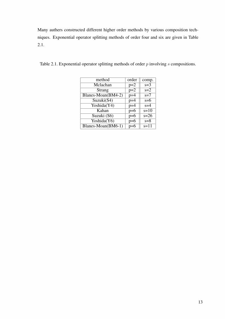
Many authers constructed different higher order methods by various composition tech-
niques. Exponential operator splitting methods of order four and six are given in Table
2.1.
Table 2.1. Exponential operator splitting methods of order p involving s compositions.
method order comp.Mclachan p=2 s=3
Strang p=2 s=2Blanes-Moan(BM4-2) p=4 s=7
Suzuki(S4) p=4 s=6Yoshida(Y4) p=4 s=4
Kahan p=6 s=10Suzuki (S6) p=6 s=26Yoshida(Y6) p=6 s=8
Blanes-Moan(BM6-1) p=6 s=11
13

CHAPTER 3
HIGHER ORDER OPERATOR SPLITTING METHODS
VIA ZASSENHAUS PRODUCT FORMULA
In the previous chapter we showed that any exponential splitting method involving
several compositions can be cast into the form (2.4). Similarly, the exponential of the
sum of two non-commutative operators A and B may be written as an infinite product as
follow,
eA+B = eAeB
∞∏n=2
eDn (3.1)
which is known as the Zassenhaus product. The Zassenhaus exponents Dn may be also
expressed as linear combinations a polynomial representation, and not the desired rep-
resentation in terms of the nested commutators. In the literature, several different ap-
proaches concerning the question how to calculate Zassenhaus exponents can be found.
In a number of independent papers, Dynkin (Dynkin, 1947), Specht (Specht, 1948),
Wever (Wever, 1947) provided a simple explicit construction of such commutator rep-
resentation. We use the formal power series expansion of the exponential function and
comparison technique to find the Zassenhaus exponents.
We solve the initial value problem (2.1). We assume A and B are bounded and
constant operators. From the Zassenhaus product formula we have the form (3.1), Expan-
sion of the left hand side of (3.1) yields,
e(A+B)t = I + (A + B)t +(A + B)2
2t2 +O(t3) (3.2)
and right hand side of (3.1) yields,
eAteBteD2t2 ... =
(I + At +
A2t2
2...
)(I + Bt +
B2t2
2...
)(I + D2t
2) +O(t3)
= I + (A + B)t +
(A2
2+ AB +
B2
2+ D2
)t2 +O(t3) (3.3)
14
By comparing the (3.2) and (3.3), D2 can be found as,
D2 = −1
2[A,B]. (3.4)
We use the following expansions to find the value of D3
eAteBt = (I + At +A2t2
2+
A3t3
6+ ...)(I + Bt +
B2t2
2+
B3t3
6+ ...) (3.5)
and
eD2t2eD3t3 = (I + D2t2 + D3t
3) +O(t4) (3.6)
The right hand side of (3.1) can be expand as follows,
eAteBteD2t2eD3t3 ... = I + (A + B)t +
(A2
2+
B2
2+ AB + D2
)t2
+
(A3
6+
B3
6+
A2B
2+
AB2
2+ (A + B)D2 + D3
)t3
+O(t4) (3.7)
and the left hand side of (3.1) yields,
e(A+B)t = I + (A + B)t +(A + B)2
2t2 +
(A + B)3
6t3 +O(t4) (3.8)
By comparing the (3.7) and (3.8), D3 can be found as,
D3 =1
6[A, [A,B]]− 1
3[B, [B,A]]. (3.9)
Again, using the formal power series expansion of exponential function, we have the
15
following form,
e(A+B)t =∞∑
k=0
1
k!(A + B)ktk = I + (A + B)t
+(1
2A2 +
1
2AB +
1
2BA +
1
2B2)t2 + ....
= (I +At
2+ ...)(I + Bt + ...)(I +
At
2+ ...)
∞∏n=3
(eDntn)
= eAt2 eBe
At2 eD3t3eD4t4 .... (3.10)
Our aim is to compute the polynomials D3 which is a function of commutators
[., [[., ]]]. By comparing the exact solution given in (3.10) with the expansion up to the
order O(t4), given in the following equation,
eAt/2eBteAt/2eD3t2 ... = I + (A + B)t + (BA + B2 + AB + A2
2)t2
+(BAA
8+
BBA
4+
A3
8+
ABA
4)τ 3
+(ABB
4+
AAB
8+ D3)t
3 +O(t4) (3.11)
D3 can be found as,
D3 =1
24[A, [A,B]]− 1
12[B, [B, A]]. (3.12)
Our aim is to improve the accuracy and modify the algorithm for better perfor-
mance. We first simply explain the basic of idea obtaining higher order result by lower
order method in the following example, we then carry this approach in order to develop a
higher order operator splitting method. Consider the scalar equation:
y′(t) = f(y), y(0) = y0 (3.13)
16
The exact solution near initial condition is given by the Taylor series expansion as follows,
y(t) = y0 + tf(y0) +t2f ′(y0)f(y0)
2!+ ...... (3.14)
Next, suppose f(y) is a linear function, f(y) = ay, we then have
y(t) = (1 + at +a2t2
2!+ ......)y0. (3.15)
Numerical approximation of this problem on the interval [0, t] by lower order explicit
Euler Method is
yapprox(t) = (1 + at)y0. (3.16)
After the initial condition is accelerated as
y0 = (1 + wt2)y0, (3.17)
the numerical approximation of the problem can be found by this initial condition in
a higher order accuracy. Here, the relaxation constant w = a2t2
2!can be obtained by
comparing the exact and approximate solution given in (3.14) and (3.17), respectively.
We then have a second order accuracy in the solution by a first order method,
yapprox(t) = (1 + at +a2t2
2!)y0 (3.18)
We exhibit our approach in Figure (3.1). Here, y0 is given initial condition and y0 is
accelerated initial condition. By applying low order method to the initial value problem
with the initial condition y0 yield the higher order result yapp(t).
17
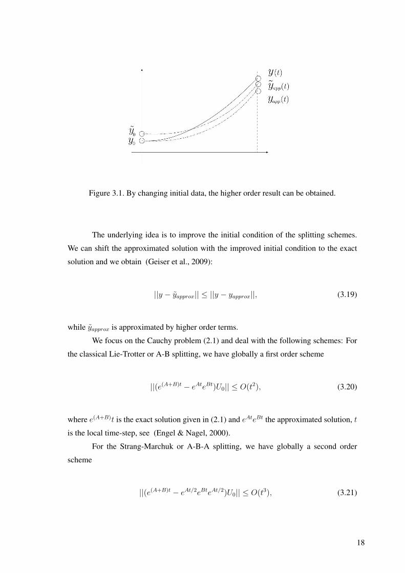
Figure 3.1. By changing initial data, the higher order result can be obtained.
The underlying idea is to improve the initial condition of the splitting schemes.
We can shift the approximated solution with the improved initial condition to the exact
solution and we obtain (Geiser et al., 2009):
||y − yapprox|| ≤ ||y − yapprox||, (3.19)
while yapprox is approximated by higher order terms.
We focus on the Cauchy problem (2.1) and deal with the following schemes: For
the classical Lie-Trotter or A-B splitting, we have globally a first order scheme
||(e(A+B)t − eAteBt)U0|| ≤ O(t2), (3.20)
where e(A+B)t is the exact solution given in (2.1) and eAteBt the approximated solution, t
is the local time-step, see (Engel & Nagel, 2000).
For the Strang-Marchuk or A-B-A splitting, we have globally a second order
scheme
||(e(A+B)t − eAt/2eBteAt/2)U0|| ≤ O(t3), (3.21)
18
where e(A+B)t is the exact solution given in (2.1) and eAt/2eBteAt/2 the approximated
solution, t is the local time-step, see (Strang, 1968).
In classical operator splitting errors, we have often the problem of improving the
lower order methods, see (Sheng, 1993). One helpful method is to improve the initial
condition by a weighted function, see Figure (3.1).
We derive a weighted function based on the initial conditions:
||U(t)−W (t)Un|| ≤ O(tm) (3.22)
where U(t) is the operator for the classical function, e.g. W (t) = exp(At) exp(Bt) for
the A-B splitting.
It can be improved by
||U(t)−W (t)Un|| ≤ O(tm+p) (3.23)
where Un = W (t)Un and W (t) is the operator for weighted function, see e.g. Zassenhaus
method, (Scholz & Weyrauch, 2006).
3.1. Higher Order Lie-Trotter Splitting by Accelerating theSubproblems Via Weighted Polynomials
We gave the algorithm of the Lie-trotter splitting in the previous chapter and
showed that the Lie-trotter splitting is a first order method. The order of the method
may be increase by the following theorems.
Theorem 3.1 We solve the initial value problem (2.10), (2.11) on the subinterval [0,t].
We assume bounded and constant operators A and B. The consistency error of the Lie-
Trotter splitting is O(t), then we can improve the error of the Lie-Trotter splitting scheme
to O(t2) by multiplied by the initial condition with the weight w2 = I + D2t2.
Proof The splitting error of Lie-Trotter splitting or A-B splitting is
ρ = exp((A + B)t)− exp(At) exp(Bt) (3.24)
= −(1
2[A,B])t2 (3.25)
19
The coefficient of t2 given in the expansion
e(A+B)t = eAteBteD2t2 +O(t3) (3.26)
is
D2 +(A + B)2
2!− ρ,
thus, if we choose D2 = ρ, the splitting error becomes O(t3). ¤
Theorem 3.2 We solve the initial value problem (2.10) and (2.11) on the subinterval
[0,t]. The consistency error of the A-B splitting is O(t), then we can improve the error of
the A-B splitting scheme to O(tp), p > 1 by improving the starting conditions U0 as
U0 = (
p∏j=2
exp(Djtj))U0
where Dj is called as Zassenhaus exponents, thus local splitting error of A-B splitting
method can be read as follows:
ρ = (exp(t(A + B))− exp(tB) exp(tA))usp (3.27)
= DT tp+1 +O(tp+2)
where DT is a function of Lie brackets of A and B.
Proof Let us consider the subinterval [0, t], where t is time step size, the solution of the
subproblem (2.10) is:
u(t) = exp(At)U0 (3.28)
20
after improving the initialization we have
u(t) = exp(At)(
p∏j=2
exp(Djtj))U0 (3.29)
the solution of the subproblem (2.11) becomes
v(t) = exp(Bt) exp(At)(
p∏j=2
exp(Djtj))U0 (3.30)
= exp((B + A)t)U0 +O(tp+1)
¤
3.2. Higher Order Strang Splitting by Accelerating the SubproblemsVia Weighted Polynomials
In order to obtain higher order Strang splitting, we present the idea of the Weighted
Polynomials in the following theorem:
Theorem 3.3 We solve the initial value problem (2.28), (2.29) and (2.30) on the subinter-
val [0,t]. We assume bounded and constant operators A and B. The consistency error of
the Strang splitting is O(t2), then we can improve the error of the Strang splitting scheme
to O(t3) by multiplied by the initial condition with the weight w3 = I + D3t3.
Proof The splitting error of Strang splitting or A-B-A splitting is
ρ = exp((A + B)t)− exp(At/2) exp(Bt) exp(At/2) (3.31)
= (1
24[B, [B, A]]− 1
12[A, [A,B]])t3 (3.32)
The coefficient of t3 given in the expansion
e(A+B)t = eAt2 eBe
At2 eD3t3 +O(t4) (3.33)
21
is
D3 +(A + B)3
3!− ρ, (3.34)
thus, if we choose D3 = ρ, the splitting error becomes O(t3). ¤
Theorem 3.4 We solve the initial value problem (2.28), (2.29) and (2.30) on the subinter-
val [0,t]. We assume bounded and constant operators A and B. The consistency error of
the Strang splitting is O(t2), then we can improve the error of the Strang splitting scheme
to O(tp), p > 2 by applying the following steps:
• Step 1: Improve the starting conditions u(0) = U0 as
u(0) = (
p∏j=2
exp(Djtj))U0
where Dj is called as Zassenhaus exponents,
• Step 2 : Accelerate v(0) as
v(0) = e−Atu(t/2),
• Step 3: Accelerate w(t/2) as
w(t/2) = eAt/2v(t),
thus the order of the A-B-A splitting method can be read as follows
e(At)/2eBte(At)/2 = e(A+B)t +O(tp+1). (3.35)
Proof Let us consider the subinterval [0, t], the solution of the subproblem (2.28) is:
u(t) = eAtU0 (3.36)
22
after improving the initialization we have
u(t) = eAt(
p∏j=2
exp(Djtj))U0. (3.37)
Next accelerate u(t) as
u(t) = e−Atu(t) (3.38)
the solution of the subproblem (2.29) becomes
v(t) = eBtu(t/2) (3.39)
= eBte−At/2eAt/2(
p∏j=2
exp(Dj(t/2)j))U0 (3.40)
or
v(t) = eBt(
p∏j=2
exp(Dj(t/2)j))U0 (3.41)
since [-A/2, A/2]=0. Finally, the acceleration of v(t) is given by the equation
v(t) = eAt/2eBt(
p∏j=2
exp(Dj(t/2)j))U0, (3.42)
then the solution of the subproblem (2.29) becomes
w(t) = eAt/2eAt/2eBt(
p∏j=2
exp(Dj(t/2)j))U0 (3.43)
23
or
w(t) = eAteBt(
p∏j=2
exp(Dj(t/2)j))U0 (3.44)
since [A/2, A/2]=0. This can be rewritten as
w(t) = eAteBt(
p∏j=2
exp(Dj(t)j))U0 (3.45)
= exp((A + B)t) +O(tp+1). (3.46)
where Dp = 12p Dj with the help of the Zassenhaus product formula. ¤
24
CHAPTER 4
CONSISTENCY ANALYSIS OF THE OPERATOR
SPLITTING METHODS
In the previous chapter, we obtained modified Lie-Trotter and Strang splitting
methods by accelerating the initial condition with via Zassenhaus product formula. In this
chapter we will obtain the errors for the operator splitting by using Zassenhaus product
formula for bounded operators and prove the the consistency of operator splitting methods
for unbounded operators by using C0-semigroup approach.
4.1. Consistency Analysis of the Operator Splitting Methods Basedon Zassenhaus Product Formula
In this section, we analyze the consistency and the order of the operator split-
ting methods by the means of the Zassenhaus product formula. We consider the Cauchy
problem (2.1) for linear bounded operators A and B.
The exact solution of (2.1) is given by
U(t) = e(A+B)tU0, t ≥ 0. (4.1)
As the exact solution operator EA+B is linear with respect to the initial value, we write
U(t) = EA+B(h)U0 = e(A+B)tU0, t ≥ 0. (4.2)
Let us divide the time interval [0, T ] of the problem into N subintervals of equal length
h = tn+1− tn, n = 0, 1, ..., N −1 the approximate solution Un+1 of U(tn+1) is computed
as Un+1 = ΦA+B(h)Un where, ΦA+B is the split solution operator.
In connection with the consistency of a splitting we give the definition of the
consistency.
25
Definition 4.1 The splitting method is called consistent of order p on [0, T ] if,
limh→0
sup0≤tn≤T−h
‖EA+B(h)U(t)− ΦA+B(h)U(t)‖h
= 0 (4.3)
and
ρh = sup0≤tn≤T−h
‖EA+B(h)U(t)− ΦA+B(h)U(t)‖h
= O(hp), p > 0, (4.4)
4.1.1. Consistency of the Lie-Trotter Splitting Based on ZassenhausProduct Formula
Here we will analyze the consistency and the order of the Lie-Trotter splitting by
the means of Zassenhaus product formula for the linear bounded operators A and B in the
Banach-space X with A,B : X → X.
Theorem 4.1 Let A and B be given linear bounded operators. We consider the abstract
Cauchy problem (2.1). Lie-Trotter splitting is consistent with the order of O(t).
Proof From the Zassenhaus product formula we have the form,
e(A+B)t = eAteBteD2t2eD3t3 ..., (4.5)
where,
D2 = −1
2[A,B] (4.6)
D3 =1
6[A, [A, B]]− 1
3[B, [B, A]] (4.7)
26
For the term eD2t2eD3t3 by using the series expansion we can write,
eD2t2eD3t3 = (I + D2t2 +O(t3))(I + D3t
3 +O(t4)) (4.8)
= I + D2t2 + D3t
3 +O(t4) (4.9)
We can write the equation (4.5) as follows,
e(A+B)t = eAteBt + eAteBt(I + D2t2 + D3t
3 +O(t4)) (4.10)
Subtracting the term eAteBt from the both sides of the equation (4.10) we get,
e(A+B)t − eAteBt = eAteBt(D2t2 + D3t
3)... (4.11)
= D2t2 + (D3 + (A + B)D2)t
3 +O(t4) (4.12)
For Lie-trotter splitting we get
e(A+B)t − eAteBt = −1
2t2[A,B] +O(t3) (4.13)
The splitting error of this operator splitting method is derived as follows:
ρt =1
t(et(A+B) − eAteBt)U(t) (4.14)
The local truncation is found to satisfy,
ρt = −1
2t[A,B]U0 +O(t2), (4.15)
¤
27
4.1.2. Consistency of the Symmetrically Weighted Splitting Based onZassenhaus Product Formula
Theorem 4.2 Let, A and B be given linear bounded operators. We consider the abstract
Cauchy problem (2.1). Symmetrically weighted splitting is consistent with the order of
O(t2).
Proof First we define,
1
2e(A+B)t =
1
2eAteBteE2t2eE3t3 ... (4.16)
1
2e(B+A)t =
1
2eBteAteE2t2eE3t3 ... (4.17)
where,
E2 = −1
2[A,B] (4.18)
E2 = −E2 (4.19)
E3 =1
6[A, [A,B]]− 1
3[B, [B,A]] (4.20)
E3 =1
6[B, [B,A]]− 1
3[A, [A,B]] (4.21)
We get the following by subtracting the summation of equations (4.16) and (4.17) from
the term e(A+B)t,
(e(A+B)t − 1
2(eAteBt + eBteAt)) =
1
2(I + (A + B)t)(E2t
2 + E3t3)
+1
2(I + (A + B)t)(E2t
2 + E3t3)
+O(t4) (4.22)
Since E2 = −E2 we have,
(e(A+B)t − 1
2(eAteBt + eBteAt)) =
1
2(E3 + E3) +O(t4) (4.23)
(4.24)
28
where,
1
2(E3 + E3) = − 1
12([A, [A, B]] + [B, [B,A]]) (4.25)
The truncation error is,
ρt = − 1
12t2([A, [A,B]] + [B, [B, A]])U0 +O(t3) (4.26)
¤
4.1.3. Consistency of the Strang Splitting Based on ZassenhausProduct Formula
Theorem 4.3 Let, A and B be given linear bounded operators. We consider the abstract
Cauchy problem (2.1). Strang splitting is consistent with the order of O(t2).
Proof The exact solution of the (2.1)can be rewritten as follows,
e(A+B)t = e(A+B)t/2+(B+A)t/2 (4.27)
= e(A+B)t/2e(B+A)t/2 (4.28)
Our aim is to show that the consistency error of the Strang Splitting by using Zassenhaus
product formula. Let us consider ,
e(A+B)t/2 = eAt/2eBt/2eF2t2eF3t3 ... (4.29)
e(B+A)t/2 = eBt/2eAt/2eF2t2eF3t3 ... (4.30)
where,
F2 = −1
2
[A
2,B
2
](4.31)
F2 = −F2 (4.32)
29
F3 =1
6
[A
2,
[A
2,B
2
]]− 1
3
[B
2,
[B
2,A
2
]](4.33)
F3 =1
6
[B
2,
[B
2,A
2
]]− 1
3
[A
2,
[A
2,B
2
]](4.34)
By a series expansion we get,
e(A+B)t/2 = eAt/2eBt/2(I + F2t2 + F3t
3 +O(t4)) (4.35)
e(B+A)t/2 = eBt/2eAt/2(I + F2t2 + F3t
3 +O(t4)) (4.36)
and we have,
e(A+B)t/2 = eAt/2eBt/2
+ eAt/2eBt/2(F2t2 + F3t
3 +O(t4)) (4.37)
e(B+A)t/2 = eBt/2eAt/2
+ eBt/2eAt/2(F2t2 + F3t
3 +O(t4)) (4.38)
Multiplying the equations (4.37) and (4.38) we get,
e(A+B)t = eAt/2eBt/2eBt/2eAt/2
+ eAt/2eBt/2eBt/2eAt/2(F2t2 + F3t
3)
+ eAt/2eBt/2(F2t2 + F3t
3)eBt/2eAt/2
+O(t4) (4.39)
Using the series expansion,
eAt/2eBt/2 = (I +At
2+
A2t2
8+ ...)(I +
Bt
2+
B2t2
8+ ...) (4.40)
= I +(A + B)t
2+O(t2) (4.41)
30
After some calculations equation (4.39) can be written in the following form,
(e(A+B)t − eAt/2eBteAt/2) = ((A + B)F2 +(A + B)
2F2 + F2
(A + B)
2+(F3 + F3))t
3 +O(t4) (4.42)
The local truncation error is,
ρt =1
24t2([A, [A,B]]− 2[B, [B, A]])U0 +O(t3) (4.43)
¤
4.2. Consistency Analysis of Operator Splitting Methods for C0
Semigroups
The consistency of the operator splitting methods is studied in the previous sec-
tion for bounded operators by means of the Zassenhaus product formula.In this section,
first we introduce the semigroup theory by giving the basic definitions, then rederive the
consistency analysis for Lie-Trotter, symmetrically Weighted and Strang Splitting for un-
bounded generators of strongly continuous semigroup.
4.2.1. Semigroup Theory
Semigroup theory is developed to solve operator ODE. Consider the following
linear equation system in ODE
∂u(t)
∂t= Au(t) (4.44)
u(0) = u0 (4.45)
where the A is matrix of constant coefficient and u is a vector function of time. It is well-
known, the solution is u(t) = eAtu(0). If A is a linear bounded operator in Banach space,
u(t) still has this form. However, in many interesting cases, it is unbounded which don’t
31
admit this form. This to some extend shows the richness of semigroup theory.
For its application, semigroup theory uses abstract methods of operator theory to
treat initial boundary value problems for linear and nonlinear equations that describe the
evolution of a system.
Definition 4.2 A one-parameter semigroup of operators over a real or complex Banach
space X is a family of bounded operators S(t), t ≥ 0 satisfy: S(t + s) = S(t)S(s) for
all t; s ≥ 0 and S(0) = I .
1. A semigroup in X, {S(t)}t≥0, is called uniformly continuous if limt→0+ S(t) = I ,
where the limit is in the topology of S(X).
2. A semigroup in X, {S(t)}t≥0, is called strongly continuous, or C0 for short, if for
every x ∈ X, limt→0+ S(t)x = x.
3. A semigroup in X, {S(t)}t≥0, is called semigroup of contractions if,
‖S(t)‖ ≤ 1 for every t ≥ 0.
Observe that in the case of a finite dimensional space, a known example of semigroups
are exponentials,
S(t) = eAt (4.46)
Also, observe that once S(t) is known, the matrix A can be determined by,
A =∂S(t)
∂t, for t = 0 (4.47)
In general case, assume u(t) is solution of (4.44), so u(t) = S(t)u0. Then, if u0 ∈ D(A)
using (4.44) we must have,
ut(0) = Au0 (4.48)
and left hand side can be written as,
ut(0) = limt→0+
S(t)u0 − u0
t(4.49)
32
This motivates the following definition,
Definition 4.3 The infinitesimal generator of a C0 semigroup is the linear operator
(A,D(A)), whose domain is given by the elements of X such that,
Ax = limt→0+
S(t)x− x
t(4.50)
exists.
Consider the linear abstract Cauchy problem (4.44)-(4.45) where A : X → X is a closed,
densely defined linear operator.Assume that A generates C0-semigroup {S(t)}t≥0. Then
there exist constants w0 ∈ R and M0 ≥ 1 such that,
‖S(t)‖ ≤ M0ew0t, t ≥ 0 (4.51)
Moreover, for any u0 ∈ D(A) (4.44) has the unique solution
u(t) = S(t)u0, t ≥ 0. (4.52)
Assume that,
A = A1 + A2, (4.53)
where A1 and A2 are generators of such C0-semigroups {S1(t)}t≥0 and {S2(t)}t≥0, which
can be approximated more easily than {S(t)}t≥0, respectively satisfying,
D(Ak) = D(Ak1) = D(Ak
2) k = 1, 2, 3 (4.54)
Let us divide the time interval (0, T ] of the problem into N sub-intervals of equal length
h = tn+1 − tn. The approximate solution Un+1s of u(tn + 1) is compute as,
Un+1s = Sspl(h)Un
s , (4.55)
33
We will concentrate on the following splitting schemes:
1. Lie-Trotter Splitting : Sspl(h) = Slie(h) = S2(h)S1(h),
2. SWS : Sspl(h) = Ssym(h) = 12(S2(h)S1(h) + S1(h)S2(h)),
3. Strang Splitting : Sspl(h) = Sstr(h) = S1(h/2)S2(h)S1(h/2).
Corresponding operator splitting method is consistent in the usual sense:
Define Th : X× [0, T − h] → X by
Th(u0, t) = S(h)u(t)− Sspl(h)(h)u(t) (4.56)
where u(t) is given by (4.52). Thus for each u0 and t, Th(u0, t) yields the local truncation
error of the corresponding splitting method.
Definition 4.4 The splitting method is said to be consistent on [0, T ] if
limh→0
sup0≤tn≤T−h
‖Th(u0, tn)‖h
= 0 (4.57)
whenever u0 ∈ B, B being some dense subspace of X.
Definition 4.5 If in the consistency relation (4.57) we have
sup0≤tn≤T−h
‖Th(u0, tn)‖h
= O(hp), p > 0, (4.58)
then the method is said to be (consistent) of order p
The following formula and lemmas will play a basic role in our investigations.
Theorem 4.4 For any C0-semigroups {S(t)}t≥0 of bounded linear operators with corre-
sponding infinitesimal generator A, we have the Taylor series expansion
S(t)x =n−1∑j=0
tj
j!Ajx +
1
(n− 1)!
t∫
0
(t− s)n−1S(s)Anxds, for all x ∈ D(An) (4.59)
34
Particularly, for n = 3, 2 and 1 we get the relations,
S(h)x = x + hAx +h2
2A2x +
1
2
h∫
0
(h− s)2S(s)A3xds, (4.60)
S(h)x = x + hAx +
h∫
0
(h− s)S(s)A2xds, (4.61)
S(h)x = x +
h∫
0
S(s)Axds, (4.62)
Lemma 4.1 Let A and B be closed linear operators from D(A) ⊂ X and D(B) ⊂ X,
respectively, into X. If D(A) ⊂ D(B), then there exists a constant C such that
‖Bx‖ ≤ C(‖Ax‖+ ‖x‖) for all x ∈ D(A). (4.63)
This implies that there exists a universal constant C by which of x ∈ Dk, k = 1, 2, 3
‖Aki x‖ ≤ C(‖Ak
j x‖+ ‖x‖) i, j = 1, 2. (4.64)
where,
Dk = D(Ak1)
⋂D(Ak
2)⋂
D(Ak) k = 1, 2, 3 dense in X (4.65)
Lemma 4.2 Let A be an infinitesimal generator of a C0-semigroup {S(t)}t≥0. Let T > 0
and n ∈ N arbitrary. If u0 ∈ D(An), then u(t) = S(t)u0 ∈ D(An) for 0 ≤ t ≤ T , and
we have
sup[0,T ]
‖Aku(t)‖ ≤ Ck(T ), k = 0, 1, ..., n (4.66)
where Ck(T ) are constants independent of h.
Proof Let z(t) = An−1u(t) = An−1S(t)u0 = S(t)An−1u0. Clearly, u0 ∈ D(An)
35
implies An−1u0 ∈ D(A). It is known from the theory of C0-semigroups [6] that then
S(t)An−1u0 ∈ D(A), i.e., An−1u(t) ∈ D(A). Consequently, u(t) ∈ D(An). Moreover,
sup[0,T ]
‖Aku(t)‖ = sup[0,T ]
‖AkS(t)u0‖ = sup[0,T ]
‖S(t)Aku0‖ ≤ Me|w|T‖Aku0‖ (4.67)
for k = 0, 1, ..., n ¤
4.2.2. Consistency of the Lie-Trotter Splitting
We need to show that the first order consistency of Lie-Trotter Splitting for C0-
semigroups. By using (4.59) for n = 2, for x ∈ D(A2) we then have,
S2(h)S1(h)x = S1(h)x + hA2S1(h)x +
h∫
0
(h− s)S2(s)A22S1(h)xds (4.68)
Substituting
S1(h)x = x + hA1x +
h∫
0
(h− s)S1(s)A21xds, (4.69)
and
S1(h)x = x +
h∫
0
S1(s)A1xds, (4.70)
into the first and second terms on the right-hand side of (4.68), respectively, we get
S2(h)S1(h)x = x + h(A1x + A2x) +
h∫
0
(h− s)S1(s)A21xds (4.71)
36
+hA2
h∫
0
S1(s)A1xds (4.72)
+
h∫
0
(h− s)S2(s)A22S1(h)xds (4.73)
On the other hand, we have
S(h)x = x + hAx +
h∫
0
(h− s)S(s)A2xds, (4.74)
so the difference is
S2(h)S1(h)x− S(h)x =
h∫
0
(h− s)S1(s)A21xds (4.75)
+hA2
h∫
0
S1(s)A1xds (4.76)
+
h∫
0
(h− s)S2(s)A22S1(h)xds (4.77)
−h∫
0
(h− s)S(s)A2xds (4.78)
Proposition 4.1 Let A, A1 and A2 be infinitesimal generators of the C0-semigroups
{S(t)}t≥0, {S1(t)}t≥0 and {S2(t)}t≥0, respectively,. Assume that (4.53) and (4.54) are
satisfied, and let T > 0. Then for all x ∈ D the relation
‖S2(h)S1(h)x− S(h)x‖ ≤ h2C(T )(‖A2x‖+ ‖Ax‖+ ‖x‖) (4.79)
holds h ∈ [0, T ], where C(T ) is a constant of independent of h.
37
Proof We estimate the terms on the right-hand side of (4.75)-(4.78). The two terms in
(4.75) and (4.78) can be estimated directly by
∥∥∥∥∥∥
h∫
0
(h− s)S1(s)A21xds
∥∥∥∥∥∥≤ M1e
|w1|h‖A21x‖
h2
2(4.80)
and
∥∥∥∥∥∥
h∫
0
(h− s)S(s)A2xds
∥∥∥∥∥∥≤ Me|w|h‖A2x‖h2
2(4.81)
The term in (4.77) is estimated by
∥∥∥∥∥∥
h∫
0
(h− s)S2(s)A22S1(h)xds
∥∥∥∥∥∥≤ M2e
|w2|h‖A22S1(h)x‖h2
2, (4.82)
but if we apply (Lemma 4.1) to compare the closed operators A22 and A2
1 we have,
‖A22S1(h)x‖ ≤ C(‖A2
1S1(h)x‖+ ‖S1(h)x‖), (4.83)
which since A21 and S1(h) commute, yields the estimate
∥∥∥∥∥∥
h∫
0
(h− s)S2(s)A22S1(h)xds
∥∥∥∥∥∥≤ M1e
|w1|hM2e|w2|hC(‖A2
1x‖+ ‖x‖)h2
2, (4.84)
For the term (4.76), using (Lemma 4.1) to compare A1 and A2, we have
∥∥∥∥∥∥hA2
h∫
0
S1(s)A1xds
∥∥∥∥∥∥≤ hC
∥∥∥∥∥∥A1
h∫
0
S1(s)A1xds
∥∥∥∥∥∥+
∥∥∥∥∥∥
h∫
0
S1(s)A1xds
∥∥∥∥∥∥
(4.85)
38
Using (4.61) twice and the fact that all semigroups commute with their generator, we get
A1
h∫
0
S1(s)A1xds = S1(h)A1x− A1x =
h∫
0
S1(s)A21xds, (4.86)
Hence we get the estimate,
∥∥∥∥∥∥hA2
h∫
0
S1(s)A1xds
∥∥∥∥∥∥≤ hC
∥∥∥∥∥∥
h∫
0
S1(s)A21xds
∥∥∥∥∥∥+
∥∥∥∥∥∥
h∫
0
S1(s)A1xds
∥∥∥∥∥∥
(4.87)
≤ h2CM1e|w1|h(‖A2
1x‖+ ‖x‖) (4.88)
Hence, adding the four estimates (4.80),(4.81), (4.84) and (4.87), we get the following,
‖S2(h)S1(h)x− S(h)x‖ ≤ h2C(T )(‖A21x‖+ ‖x‖+ ‖A2x‖+ ‖x‖) (4.89)
From Lemma 4.1 we know that we can bound ‖A21x‖ in terms of ‖A2x‖ + ‖x‖ and
similarly ‖A1x‖ in terms of ‖A2x‖+ ‖x‖. ¤
To prove the first-order consistency of the Lie-Trotter splitting, we need a uniform bound,
proportional to h2 on
‖S2(h)S1(h)u(t)− S(h)u(t)‖ (4.90)
as t runs from 0 to T − h, where u(t) = S(t)u0 is the exact solution of the original
problem (4.44)-(4.45).
Proposition (4.1), (4.64) and Lemma (4.2) imply the following
Theorem 4.5 Let the conditions of Proposition (4.1) be satisfied. Then for any u0 ∈ D
we have a uniform bound
‖S2(h)S1(h)u(t)− S(h)u(t)‖ ≤ h2C(T ) (4.91)
39
where C(T ) is a constant independent of h.
4.2.3. Consistency of the Symmetrically Weighted Splitting
Our aim is to show the second order consistency of the Symmetrically Weighted
Splitting for C0-semigroups. By using (4.59) for n = 3, for x ∈ D(A) we then have,
S2(h)S1(h)x = S1(h)x + hA2S1(h)x +h2
2A2
2S1(h)x (4.92)
+1
2
h∫
0
(h− s)2S2(s)A32S1(h)xds (4.93)
and similarly,
S1(h)S2(h)x = S2(h)x + hA1S2(h)x +h2
2A2
1S2(h)x (4.94)
+1
2
h∫
0
(h− s)2S1(s)A31S2(h)xds (4.95)
Applying (4.60), (4.61) and (4.62) for the semigroups {S1(t)}t≥0 and {S2(t)}t≥0 and
substituting the corresponding expressions into the first, second and third terms of the
right-hand side of (4.92), we get
1
2(S2(h)S1(h) + S1(h)S2(h)x) = (4.96)
x + h(A1 + A2)x +h2
2(A1 + A2)
2x (4.97)
+1
4
h∫
0
(h− s)2S1(s)A31xds (4.98)
+1
4
h∫
0
(h− s)2S2(s)A32xds (4.99)
+1
2hA2
h∫
0
(h− s)S2(s)A21xds +
1
2hA1
h∫
0
(h− s)S2(s)A22xds (4.100)
40
+1
4h2A2
2
h∫
0
S1(s)A1xds +1
4h2A2
1
h∫
0
S2(s)A2xds (4.101)
+1
4
h∫
0
(h− s)2S2(s)A32S1(h)xds +
1
4
h∫
0
(h− s)2S1(s)A31S2(h)xds (4.102)
On the other hand, we have
S(h)x = x + hAx +h2
2A2x +
1
2
h∫
0
(h− s)2S(s)A3xds (4.103)
so the difference is
1
2(S2(h)S1(h) + S1(h)S2(h)x)− S(h)x = (4.104)
+1
4
h∫
0
(h− s)2S1(s)A31xds +
1
4
h∫
0
(h− s)2S2(s)A32x (4.105)
+1
2hA2
h∫
0
(h− s)S1(s)A21xds +
1
2hA1
h∫
0
(h− s)S2(s)A22xds (4.106)
+1
4h2A2
2
h∫
0
S1(s)A1xds +1
4h2A2
1
h∫
0
S2(s)A2xds (4.107)
+1
4
h∫
0
(h− s)2S2(s)A32S1(h)xds +
1
4
h∫
0
(h− s)2S1(s)A31S2(h)xds (4.108)
−1
2
h∫
0
(h− s)2S(s)A3xds (4.109)
Proposition 4.2 Let A, A1 and A2 be infinitesimal generators of the C0-semigroups
{S(t)}t≥0, {S1(t)}t≥0 and {S2(t)}t≥0, respectively,. Assume that (4.53) and (4.54) are
satisfied, and let T > 0. Then for all x ∈ D the relation
∥∥∥∥1
2(S2(h)S1(h) + S1(h)S2(h)x)− S(h)x
∥∥∥∥ ≤ (4.110)
h3C(T )(‖A3x‖+ ‖A2x‖+ ‖Ax‖+ ‖x‖) (4.111)
41
holds h ∈ [0, T ], where C(T ) is a constant of independent of h.
Proof We estimate the terms on the right-hand side of (4.104)-(4.109). For the first
term in (4.106) by using (Lemma 4.1) we can write
∥∥∥∥∥∥1
2hA2
h∫
0
(h− s)S1(s)A21xds
∥∥∥∥∥∥≤ C
2h
∥∥∥∥∥∥A1
h∫
0
(h− s)S1(s)A21xds
∥∥∥∥∥∥(4.112)
+C
2h
∥∥∥∥∥∥
h∫
0
(h− s)S1(s)A21xds
∥∥∥∥∥∥(4.113)
Using (4.61) twice and the fact that all semigroups commute with their generator, for the
term (4.112) we obtain the estimate
C
2h
∥∥∥∥∥∥A1
h∫
0
(h− s)S1(s)A21xds
∥∥∥∥∥∥≤ M1e
|w1|h‖A31x‖
h3
4C. (4.114)
Term (4.113) can be estimated by
C
2h
∥∥∥∥∥∥
h∫
0
(h− s)S1(s)A21xds
∥∥∥∥∥∥≤ M1e
|w1|h‖A21x‖
h3
4C. (4.115)
So,
∥∥∥∥∥∥1
2hA2
h∫
0
(h− s)S1(s)A21xds
∥∥∥∥∥∥≤ M1e
|w1|h(‖A31x‖+ ‖A2
1x‖)h3
4C. (4.116)
Similarly, for the second term in (4.106) the following relation is valid,
∥∥∥∥∥∥1
2hA1
h∫
0
(h− s)S2(s)A22xds
∥∥∥∥∥∥≤ M2e
|w2|h(‖A32x‖+ ‖A2
2x‖)h3
4C. (4.117)
42
For the estimate of he first term of (4.107) on the base of (Lemma 4.1) we can write
∥∥∥∥∥∥1
4h2A2
2
h∫
0
S1(s)A1xds
∥∥∥∥∥∥≤ C
4h2
∥∥∥∥∥∥A2
1
h∫
0
(h− s)S1(s)A1xds
∥∥∥∥∥∥(4.118)
+C
4h2
∥∥∥∥∥∥
h∫
0
(h− s)S1(s)A1xds
∥∥∥∥∥∥(4.119)
where for terms (4.118) we have
C
4h2
∥∥∥∥∥∥A2
1
h∫
0
(h− s)S1(s)A1xds
∥∥∥∥∥∥=
C
4h2
∥∥∥∥∥∥
h∫
0
(h− s)S1(s)A31xds
∥∥∥∥∥∥(4.120)
≤ C
4h3M1e
|w1|h‖A31x‖ (4.121)
and for the term (4.119),
C
4h2
∥∥∥∥∥∥
h∫
0
(h− s)S1(s)A1xds
∥∥∥∥∥∥≤ C
4h3M1e
|w1|h‖A1x‖ (4.122)
Consequently,
∥∥∥∥∥∥1
4h2A2
2
h∫
0
S1(s)A1xds
∥∥∥∥∥∥≤ M1e
|w1|hC(‖A31x‖+ ‖A1x‖)h
3
4. (4.123)
In a similar way, the second term of (4.107) is estimated by
∥∥∥∥∥∥1
4h2A2
1
h∫
0
S2(s)A2xds
∥∥∥∥∥∥≤ M2e
|w2|hC(‖A32x‖+ ‖A2x‖)h
3
4. (4.124)
43
For the first term of (4.108) we can write
∥∥∥∥∥∥1
4
h∫
0
(h− s)2S2(s)A32S1(h)xds
∥∥∥∥∥∥≤ M2e
|w2|h‖A32S1(h)x‖h3
12(4.125)
≤ M2e|w2|hC(‖A3
1S1(h)x‖+ ‖S1(h)x‖)h3
12(4.126)
≤ M1e|w1|hM2e
|w2|hC(‖A31x‖+ ‖x‖)h
3
12(4.127)
Finally, in a similar manner, the second term of (4.108) is estimated by
∥∥∥∥∥∥1
4
h∫
0
(h− s)2S1(s)A31S2(h)xds
∥∥∥∥∥∥≤ (4.128)
M1e|w1|hM2e
|w2|hC(‖A32x‖+ ‖A2x‖)h
3
12. (4.129)
¤
To prove the second-order consistency of the Symmetrically weighted splitting,
we need a uniform bound, proportional to h3 on
‖1
2(S2(h)S1(h)u(t) + S1(h)S2(h)u(t))− S(h)u(t)‖ (4.130)
as t runs from 0 to T−h, where u(t) = S(t)u0 is the exact solution of the original problem
(4.44)-(4.45).
Proposition (4.2), (4.64) and Lemma (4.2) imply the following
Theorem 4.6 Let the conditions of Proposition (4.2) be satisfied. Then for any u0 ∈ D
we have a uniform bound
∥∥∥∥1
2(S2(h)S1(h)u(t) + S1(h)S2(h)u(t))− S(h)u(t)
∥∥∥∥ ≤ h3C(T ) (4.131)
where C(T ) is a constant independent of h.
44
4.2.4. Consistency of the Strang Splitting
Let us introduce the notation y = S2(h)S1(h/2), and let x ∈ D according to
(4.54). Then we can write
S1(h/2)S2(h)S1(h/2) = S1(h/2)y (4.132)
and by (4.59) we have
S1(h/2)y = y +h
2A1y +
h2
8A2
1y +1
2
h/2∫
0
(h
2− s)2S1(s)A
31yds (4.133)
Substituting
y = S1(h/2)x + hA2S1(h/2)x +h2
2A2
2S1(h/2)x (4.134)
+1
2
h∫
0
(h− s)2S2(s)A32S1(h/2)xds (4.135)
y = S1(h/2)x + hA2S1(h/2)x +
h∫
0
(h− s)S2(s)A22S1(h/2)xds (4.136)
y = S1(h/2)x +
h∫
0
S2(s)A2S1(h/2)xds (4.137)
and
y = S2(h)S1(h/2)x (4.138)
successively the terms of the right-hand side of (4.133), and the expressions
S1(h/2)x = x +h
2A1x +
h2
8A2
1x +1
2
h/2∫
0
(h
2− s)2S1(s)A
31xds (4.139)
45
S1(h/2)x = x +h
2A1x +
h/2∫
0
(h
2− s)S1(s)A
21xds (4.140)
S1(h/2)x = x +
h/2∫
0
S1(s)A1xds (4.141)
Taking into account (4.103), we obtain that
S1(h/2)S2(h)S1(h/2)x− S(h)x = (4.142)
+1
2
h/2∫
0
(h
2− s)2S1(s)A
31xds + hA2
h/2∫
0
(h
2− s)S1(s)A
21xds (4.143)
+h2
2A2
2
h/2∫
0
S1(s)A1xds +1
2
h∫
0
(h− s)2S2(s)A32S1(h/2)xds (4.144)
+h
2A1
h/2∫
0
(h
2− s)S1(s)A
21xds +
h2
2A1A2
h/2∫
0
S1(s)A1xds (4.145)
+h
2A1
h∫
0
(h− s)S2(s)A22S1(h/2)xds +
h2
8A2
1
h/2∫
0
S1(s)A1xds (4.146)
+h2
8A2
1
h∫
0
S2(s)A2S1(h/2)xds (4.147)
+1
2
h/2∫
0
(h
2− s)2S1(s)A
31S2(h)S1(h/2)xds (4.148)
−1
2
h∫
0
(h− s)2S(s)A3xds (4.149)
Proposition 4.3 Let A, A1 and A2 be infinitesimal generators of the C0-semigroups
{S(t)}t≥0, {S1(t)}t≥0 and {S2(t)}t≥0, respectively,. Assume that (4.53) and (4.54) are
satisfied, and let T > 0. Then for all x ∈ D the relation
‖S1(h/2)S2(h)S1(h/2)x− S(h)x‖ ≤ (4.150)
h3C(T )(‖A3x‖+ ‖A2x‖+ ‖Ax‖+ ‖x‖) (4.151)
46
holds h ∈ [0, T ], where C(T ) is a constant of independent of h.
Proof We estimate the terms on the right-hand side of (4.142)-(4.149) one by one. The
first term of (4.143) can be directly estimated as
1
2
∥∥∥∥∥∥
h/2∫
0
(h
2− s)2S1(s)A
31xds
∥∥∥∥∥∥≤ M1e
|w1|h/2‖A31x‖
h3
48(4.152)
For the second term of (4.143) by the use of (Lemma 4.1) we can write
∥∥∥∥∥∥hA2
h/2∫
0
(h
2− s)S1(s)A
21xds
∥∥∥∥∥∥≤ Ch
∥∥∥∥∥∥A1
h/2∫
0
(h
2− s)S1(s)A
21xds
∥∥∥∥∥∥(4.153)
+Ch
∥∥∥∥∥∥
h/2∫
0
(h
2− s)S1(s)A
21xds
∥∥∥∥∥∥(4.154)
Here by using (4.61) twice, for the first integral can be written as
A1
h/2∫
0
(h
2− s)S1(s)A
21xds =
h/2∫
0
(h
2− s)S1(s)A
31xds (4.155)
and so the term (4.153) can be estimated by
M1e|w1|h/2‖A3
1x‖h3
8C (4.156)
For the term (4.154) the following estimates holds
M1e|w1|h/2‖A2
1x‖h3
8C (4.157)
47
The first term of (4.144) we have
∥∥∥∥∥∥h2
2A2
2
h/2∫
0
S1(s)A1xds
∥∥∥∥∥∥≤ M1e
|w1|h/2(‖A31x‖+ ‖A1x‖)h
3
4(4.158)
The second term of (4.144) can be estimated as
1
2
∥∥∥∥∥∥
h∫
0
(h− s)2S2(s)A32S1(h/2)xds
∥∥∥∥∥∥≤ 1
2M2e
|w2|h‖A32xS1(h/2)‖h3
3(4.159)
From the (Lemma 4.1) we get the right-hand side of (4.159)
M1e|w1|h/2M2e
|w2|hC(‖A31x‖+ ‖x‖)h
3
6(4.160)
For the first term of (4.145) we can write
h
2
∥∥∥∥∥∥A1
h/2∫
0
(h
2− s)S1(s)A
21xds
∥∥∥∥∥∥≤ M1e
|w1|h/2‖A31x‖
h3
16(4.161)
For the second term one has
∥∥∥∥∥∥h2
2A1A2
h/2∫
0
S1(s)A1xds
∥∥∥∥∥∥≤ C
h2
2‖A2
2
h/2∫
0
S1(s)A1xds‖ (4.162)
+Ch2
2‖A2
h/2∫
0
S1(s)A1xds‖ (4.163)
which, by Lemma (4.1), is less than or equal to
M1e|w1|h/2C2(‖A3
1x‖+ ‖A21x‖+ 2‖A1x‖)h
3
4(4.164)
48
Using again Lemma (4.1), the first term of (4.146) can be estimated as
h
2
∥∥∥∥∥∥A1
h∫
0
(h− s)S2(s)A22S1(h/2)xds
∥∥∥∥∥∥(4.165)
≤ h
2C(‖A2
h∫
0
(h− s)S2(s)A22S1(h/2)xds‖) (4.166)
+‖h∫
0
(h− s)S2(s)A22S1(h/2)xds‖ (4.167)
≤ M2e|w2|hM1e
|w1|h/2C2(‖A31x‖+ ‖A2
1x‖+ 2‖A1x‖)h3
4(4.168)
For the second term of (4.146) we have
h2
8
∥∥∥∥∥∥A2
1
h/2∫
0
S1(s)A1xds
∥∥∥∥∥∥≤ M1e
|w1|h/2‖A31x‖
h3
16(4.169)
We estimate the (4.147) as
h2
8
∥∥∥∥∥∥A2
1
h∫
0
S2(s)A2S1(h/2)xds
∥∥∥∥∥∥
≤ h2
8C
∥∥∥∥∥∥A2
2
h∫
0
S2(s)A2S1(h/2)xds
∥∥∥∥∥∥+
h2
8C
∥∥∥∥∥∥
h∫
0
S2(s)A2S1(h/2)xds
∥∥∥∥∥∥
≤ h3
8C2M2e
|w2|h‖A32S1(h/2)x‖+
h3
8C2M2e
|w2|h‖A2S1(h/2)x‖
≤ M1e|w1|h/2M2e
|w2|hC2(‖A31x‖+ ‖A1x‖+ 2‖x‖)h
3
8(4.170)
and the (4.148)
1
2
∥∥∥∥∥∥
h/2∫
0
(h
2− s)2S1(s)A
31S2(h)S1(h/2)xds
∥∥∥∥∥∥≤ (4.171)
≤ h3
48M1e
|w1|h/2C(‖A32S2(h)S1(h/2)x‖+ ‖S2(h)S1(h/2)x‖) (4.172)
49
Here
‖A32S2(h)S1(h/2)x‖ ≤ M2e
|w2|h‖A32S1(h/2)x‖ (4.173)
≤ M2e|w2|hC(‖‖A3
1S1(h/2)x‖+ ‖S1(h/2)x‖). (4.174)
Therefore
1
2
∥∥∥∥∥∥
h/2∫
0
(h
2− s)2S1(s)A
31S2(h)S1(h/2)xds
∥∥∥∥∥∥≤ (4.175)
M1e|w1|h/2M2e
|w2|hM1e|w1|h/2(C2(‖A3
1x‖+ ‖x‖) + C‖x‖)h3
48(4.176)
Finally, for the term (4.149) we have
1
2
∥∥∥∥∥∥
h∫
0
(h− s)2S(s)A3xds
∥∥∥∥∥∥≤ 1
2Me|w|h‖A3x‖h3
3. (4.177)
¤
Proposition (4.3), (4.64) and Lemma 4.2 imply the following
Theorem 4.7 Let the conditions of Proposition (4.3) be satisfied. Then for any u0 ∈ D
we have a uniform bound
‖S1(h/2)S2(h)S1(h/2)x− S(h)x‖ ≤ h3C(T ) (4.178)
where C(T ) is a constant independent of h.
50
CHAPTER 5
STABILITY ANALYSIS FOR OPERATOR SPLITTING
METHODS
In this chapter, we will discuss the stability analysis of the operator splitting meth-
ods for ODE systems and PDE problems, such that nonlinear KdV equation. For PDE
sense we will use the Von-Neumann stability analysis. General approach to Von-Neumann
stability analysis for Lie-Trotter and Strang splitting will be discussed.
5.1. Stability for Linear ODE Systems
In this section, we take a look at properties of linear systems of ODEs and in
particular at influence of perturbations at such systems.
Consider the initial value problem,
∂U(t)
∂t= AU(t), with t ∈ [0, T ], U(0) = U0, (5.1)
with given matrix A ∈ Rm×m. The solution of the equation (5.1) can be written as,
U(t) = etAU0. (5.2)
Consider also a perturbed problem,
∂U(t)
∂t= AU(t) + δ(t), with t ∈ [0, T ], U(0) = U0, (5.3)
Then for ε(t) = U(t)− U(t) we find by the variation of constant formula that,
ε(t) = etAε(0) +
∫ t
0
e(t−s)Aδ(s)ds, (5.4)
51
which leads to the norm estimate
‖ε(t)‖ ≤ ‖etA‖‖ε(0)‖ +
∫ t
0
‖e(t−s)A‖ds max0≤s≤t
‖δ(s)‖. (5.5)
Consequently, if we have the following stability inequality
‖etA‖ ≤ Ketw for all t ≥ 0, (5.6)
with constants K > 0 and w ∈ R, then we obtain
‖ε(t)‖ ≤ Ketw‖ε(0)‖+K
t(etw − 1) max
0≤s≤t‖δ(s)‖, (5.7)
with convention (etw − 1)/w = t in case w = 0. This inequality shows that the overall
error ‖ε(t)‖ can be bounded in terms of the initial error ‖ε(0)‖ and perturbations ‖δ(s)‖,
0 ≤ s ≤ t.
In general, the term stability will be used to indicate that small perturbations give
a small overall effect. We now take a closer look at bounds for ‖etA‖. Suppose that A is
diagonalizable, A = PΛP−1, where Λ = diag(λk) and that the vector norm is absolute.
Then it follows that,
‖etA‖ ≤ ‖P‖‖Λ‖‖P−1‖ = cond(P ) max1≤k≤m
|etλk |. (5.8)
Consequently, if we know that cond(P ) = ‖P‖‖P−1‖ ≤ K and Reλk ≤ w, then (5.6)
follows with
w = max1≤k≤m
|etλk |. (5.9)
In particular, if A is normal matrix, then the matrix of eigenvectors P is unitary.
Since etA = PetΛP−1 the matrix etA is also normal. Thus with the normal matrices A we
52
have
‖etA‖2 = max1≤k≤m
|etλk |. (5.10)
Assume for A, two-term splitting in (5.1),
A = A1 + A2 (5.11)
The solution of (5.1) is given by
U(tn+1) = etAU(tn) (5.12)
where t = tn+1− tn on each subintervals [tn, tn+1], where n = 0, 1, ..., N − 1. If we wish
to use only A1 and A2 separately, instead of the full A, then (5.12) can be approximated
by
Un+1 = etA2etA1Un (5.13)
with Un approximating U(tn). With regard to stability, if we have ‖etAk‖ ≤ 1, k = 1, 2,
then it follows trivially that ‖Un+1‖ ≤ ‖Un‖ for the splitting (5.13). General stability
results under the weaker assumption that ‖etAk‖ ≤ K for 0 ≤ t ≤ T with a constant
K ≥ 1 seem unknown. However, in practice the splitting appears to be stable provided
the sub-steps themselves are stable.
In general, if the matrix A is not normal, an estimate of cond(U) in some suitable
norm maybe difficult to obtain. For this reason we will look a more general concept to
obtain bounds for ‖etA‖. A useful concept for stability results with non-normal matrices
is the logarithmic norm of a matrix A in Rm×m, defined as
µ(A) = limt↓0
‖I + tA‖t
. (5.14)
In terms of logarithmic matrix norms, ‖etAk‖ ≤ 1 means that µ(Ak) ≤ 0. This implies
53
µ(A1 + A2) ≤ 0 and therefore ‖et(A1+A2)‖ ≤ 1, so the system will be stable.
5.2. Stability Analysis for PDE
In order to determine the Courant-Friedrichs-Levy condition for the stability of an
explicit solution of a PDE the Von Neumann stability analysis is used. A very versatile
tool for analysing stability is the Fourier method developed by Von Neumann. Here initial
values at mesh points are expressed in terms of a finite Fourier series, and we consider the
growth of individual Fourier components. We do not need to find eigenvalues, or matrix
norms.
A unique representation of the function U(x) can be expressed as,
U(x) =1√2π
∫ ∞
−∞U(ξ)eiξxdξ (5.15)
Consider a trial solution at x,
U(x, t) = U(t)eikx (5.16)
We can write the Unj and Un+1
j as follows,
Unj = U(xj, tn) = Uneikjh (5.17)
Un+1j = U(xj, tn+1) = Un+1eikjh (5.18)
The amplification factor is so called because its magnitude is the amount of the amplitude
of each frequency in the solution given by,
ρ(ξ) =Un+1
Un(5.19)
Where ξ = kjh. If |ξ| ≤ 1 then the solution dampened. If |ξ| > 1 the solution grows in
amplitude and becomes unstable.
We illustrate the method by considering the particular example. Through the use
54
of Fourier transform the determination of the stability of a scheme is reduced to relatively
simple algebraic consideration.
We consider the following problem parabolic problem:
ut = Duxx, (5.20)
Let xi = i∆x and tn = n∆t, i = 1, ..., M − 1 n = 0, ..., N Respectively ∆x =
1M
∆t = 1N
are the regular spatial end time step sizes. The discrete representation of
(5.20) over each time interval [tn, tn + ∆t] is as follows,
Un+1i − Un
i
∆t=
D
∆x2(Un+1
i+1 − 2Un+1i + Un+1
i−1 ) (5.21)
Let say D∆t∆x2 = r. Rearranging the terms (5.21) according to the time level, then
−rUn+1i+1 + (1 + 2r)Un+1
i − rUn+1i−1 = Un
i (5.22)
The discrete Fourier transform of (5.22) is given by,
(−reiξ + (1 + 2r)− re−iξ)Un+1 = Un (5.23)
After simplification (5.23) reduce to
(1 + 4r sin2 ξ/2)Un+1 = Un (5.24)
and amplification factor corresponding to (5.24) is given by,
ρ(ξ) =1
1 + 4r sin2 ξ/2(5.25)
55
The stability of the solution obtained by the diffusion operator satisfies that,
|ρ(ξ)| < 1 (5.26)
for any value of r > 0 for any positive scalar coefficient of the diffusion operator.
5.3. Stability Analysis of the Non-linear KdV Equation
In this section, we first give the numerical algorithms then present the Von Neu-
mann stability analysis for the nonlinear KdV equation by appling Lie-Trotter and Strang
splitting methods and give the stability conditions related to these methods.
In 1895, Korteweg and de Vries formulated the equation
Ut − 6UUx + Uxxx = 0 (5.27)
which models Russell’s observation.The term UUx describes the sharpening of the wave
and Uxxx the dispersion. Let xi = i∆x and tn = n∆t, i = 1, ...,M − 1 n = 0, ..., N
Respectively ∆x = 1M
∆t = 1N
are the regular spatial end time step sizes. The first
step towards solving (5.27) is to consider the fractional splitting method, which can be
expressed as follows:
ut = −uxxx , t ∈ [tn, tn + ∆t] , (5.28)
vt = 6uvx, t ∈ [tn, tn + ∆t] , v(tn) = u(tn + ∆t) . (5.29)
We substitute the solution of the equation (6.36) for u in (6.37),
We imply the semi-discretisation for (5.27) using the central difference approxi-
mation. The finite difference approximation of the operators (5.27) are given by,
(6u∂u
∂x− ∂3u
∂x3)(xi,t) = 6u
1
2∆x(ui+1(t)− ui−1(t))
− 1
2∆x3(ui+2(t)− 2ui+1(t) + 2ui−1(t)− ui−2(t)) (5.30)
56
We will take u as a constant in here, for i = 1, ..., N We obtain the following system of
the first order differential equation,
ut = Au (5.31)
vt = Bv (5.32)
where A and B are global matrices of coefficients resulting from he discretisation of
−uxxx and vx
A = − 1
2∆x3[1 − 2 2 − 1] (5.33)
B = 6c1
2∆x[−1 0 1] (5.34)
We will obtain the following system of first order differential equation given by,
∂u∗
∂t= (A + B)u∗ (5.35)
The exact solution of (5.35) satisfies the matrix exponential function of the matrices A
and B given by,
u∗(t + ∆t) = e∆t(A+B)u∗(t) (5.36)
where ∆t is the time step for the simulation of of the solution through [0, T ]
5.3.1. Algorithm 1 (First Order Splitting Method)
Over the time interval [tn, tn + ∆t]
• Step1:
u(tn + ∆t) = e∆tAu(tn) with u(tn) = u∗(tn) (5.37)
57
• Step2:
v(tn + ∆t) = e∆tBv(tn) with v(tn) = u(tn + ∆t) (5.38)
• Step3:
u∗(tn + ∆t) = v(tn + ∆t) (5.39)
• Step4: If T < (n + 1)∆t go to Step1, otherwise stop.
The recurrence solution given by (5.37) and (5.38) will be estimated using the Pade’
approximation for e∆tA and e∆tB, respectively (Daoud, 2007)
e∆tA = (I −∆tA)−1 + O(∆t2) , (5.40)
e∆tB = (I −∆tB)−1 + O(∆t2),
which is locally second order approximation in time O(∆t2).Therefore,
e∆t(A+B) ' e∆tAe∆tB ' (I −∆tA)−1(I −∆tB)−1O(∆t2) ' (I −∆tA)−1 (5.41)
We could easily observe that
u(tn + ∆t) = e∆tAe∆tBu(tn) ' e∆t(A+B) (5.42)
The discrete presentation of (5.37) and (5.38) using (5.57) over each time interval [tn, tn+
∆t] are as follows
un+1i − un
i
∆t= − 1
2∆x3(un+1
i+2 − 2un+1i+1 + 2un+1
i−1 − un+1i−2 ) , (5.43)
vn+1i − vn
i
∆t=
1
2∆x(vn+1
i+1 − vn+1i−1 )
58
Let 6c∆t2∆x
= R and ∆t2∆x3 = r Rearranging the terms of (5.43) according to the time level,
then
run+1i+2 − 2run+1
i+1 + 2run+1i−1 − run+1
i−2 + un+1i = un
i , (5.44)
−Rvn+1i+1 + vn+1
i + Rvn+1i−1 = vn
i
Next, we will investigate the stability analysis of Lie-Trotter splitting.
5.3.2. Stability Analysis of the Lie-Trotter Splitting
Theorem 5.1 For any ∆t and ∆x the First Order Splitting Method (Lie-Trotter Splitting)
is stable in `2 norm.
Proof For stability of the `2 norm we will consider the Von-Neumann stability analysis
and using the discrete Fourier transform. The discrete Fourier transform is given by
uneiξ = run+1e(i+2)ξ − 2run+1e(i+1)ξ + 2run+1e(i−1)ξ (5.45)
+ ru(d)n+1e(i−2)ξ + u(d)n+1eiξ
vneiξ = −Rvn+1e(i+1)ξ + vn+1eiξ + Rvn+1e(i−1)ξ
rearanging the terms in (5.45) we get,
un = (re2iξ − 2reiξ + 2re−iξ − re−2iξ + 1)un+1 (5.46)
vn = (−Reiξ + 1 + Re−iξ)vn+1
After simplification (5.46) reduce to ,
(1 + 2irsinξ(cosξ − 1))un+1 = un (5.47)
(1 + 2iRsinξ)vn+1 = vn
59
and the amplification factors corresponding to (5.47) are given by
ρB(ξ) =1
(1 + 2iRsinξ)ρA(ξ) =
1
(1 + 2irsinξ(cosξ − 1))(5.48)
for stability of the solution corresponding to the convection operator it is easily observed
that
|ρB(ξ)| < 1 (5.49)
for any value of R.The stability of the solution of the diffusion operator satisfies
|ρA(ξ)| <∣∣∣∣
1
(1 + 2irsinξ(cosξ − 1))
∣∣∣∣ < 1 (5.50)
for any r > 0. Since the solution of (5.27) is represented by the splitting operators,
operators are given by (5.59).Therefore the amplification factor corresponding to discrete
Fourier transform corresponding to the discretisation of (5.27) is given
ρ(ξ) = ρA(ξ)ρB(ξ) (5.51)
and
|ρ(ξ)| < |ρA(ξ)||ρB(ξ)| < 1 (5.52)
Therefore the solution of(5.27) using the first order splitting (Lie-Trotter) is uncondition-
ally stable for any positive scalar coefficient of the given operators. ¤
5.3.3. Algorithm 2 (Second Order Splitting Method)
Over the time interval [tn, tn + ∆t]
60
• Step1
u(tn + ∆t/2) = e(∆t/2)Au(tn) with u(tn) = u∗(tn) (5.53)
• Step2
v(tn + ∆t) = e∆tBv(tn) with v(tn) = u(tn + ∆t/2) (5.54)
• Step3
w(tn + ∆t/2) = e(∆t/2)Aw(tn) with w(tn + ∆t/2) = v(tn + ∆t) (5.55)
• Step4
u∗(tn + ∆t) = w(d)(tn + ∆t) (5.56)
• Step5 If T < (n + 1)∆t go to Step1, otherwise stop.
We will be estimated using the Pade’ approximation for e∆t/2A and e∆tB, respectively
e(∆t/2)A = (I − (∆t/2)A)−1 + O(∆t2) (5.57)
e∆tB = (I −∆tB)−1 + O(∆t2),
Therefore,
e∆t(A+B) ' e(∆t/2)Ae∆tBe(∆t/2)A (5.58)
' (I − (∆t/2)A)−1(I −∆tB)−1(I − (∆t/2)A)−1O(∆t2)
' (I −∆t(A + B))−1
61

From the above discussion we could easily observe that,
u(tn + ∆t) = e(∆t/2)Ae∆tBe(∆t/2)Au(tn) ' e∆t(A+B) (5.59)
The discrete presentation of the Algorithm 2 over the each time interval are as follows:
un+1/2i − un
i
∆t= − 1
2∆x3(u
n+1/2i+2 − 2u
n+1/2i+1 + 2u
n+1/2i−1 − u
n+1/2i−2 ) (5.60)
vn+1i − vn
i
∆t=
1
2∆x(vn+1
i−1 − vn+1i+1 )
wn+1/2i − wn
i
∆t= − 1
2∆x3(w
n+1/2i+2 − 2w
n+1/2i+1 + 2w
n+1/2i−1 − w
n+1/2i−2 )
Let 6c ∆t2∆x
= R and ∆t2∆x3 = r Rearranging the terms of (5.43) according to the time level,
then
run+1/2i+2 − 2ru
n+1/2i+1 + 2ru
n+1/2i−1 − ru
n+1/2i−2 + u
n+1/2i = un
i (5.61)
−Rvn+1i+1 + vn+1
i + Rvn+1i−1 = vn
i
rwn+1/2i+2 − 2rw
n+1/2i+1 + 2rw
n+1/2i−1 − rw
n+1/2i−2 + w
n+1/2i = wn
i
Next we will investigate the stability analysis for Strang splitting.
5.3.4. Stability Analysis of the Strang Splitting
Theorem 5.2 For any ∆t and ∆x The Second Order Splitting Method (Strang Splitting)
is stable in `2 norm.
Proof For any ∆t and ∆x Strang Splitting is stable in `2 norm.We will consider the
Von Neuman stability analysis using the discrete Fourier transform.The discrete Fourier
transform (5.61)is given by
uneiξ = run+1/2e(i+2)ξ − 2run+1/2e(i+1)ξ + 2run+1/2e(i−1)ξ (5.62)
+ run+1/2e(i−2)ξ + un+1/2eiξ
62
vneiξ = −Rvn+1e(i+1)ξ + vn+1eiξ + Rvn+1e(i−1)ξ
wneiξ = rwn+1/2e(i+2)ξ − 2rwn+1/2e(i+1)ξ + 2rwn+1/2e(i−1)ξ
+ rwn+1/2e(i−2)ξ − wn+1/2eiξ
rearanging the terms in (5.62)we get,
un = (re2iξ − 2reiξ + 2re−iξ − re−2iξ + 1)vn+1/2 (5.63)
vn = (−Reiξ + 1 + Re−iξ)un+1
wn = (re2iξ − 2reiξ + 2re−iξ − re−2iξ + 1)wn+1/2
After simplification (5.63) reduce to ,
(1 + 2irsinξ(cosξ − 1))un+1/2 = un (5.64)
(1 + 2iRsinξ)un+1 = un
(1 + 2irsinξ(cosξ − 1))wn+1/2 = wn
and the amplification factors corresponding to (5.64) are given by
ρB(ξ) =1
(1 + 2iRsinξ)ρA/2(ξ) =
1
(1 + 2irsinξ(cosξ − 1))(5.65)
for stability of the solution corresponding to the operator it is easily observed that
|ρB(ξ)| < 1 (5.66)
for any value of R.The stability of the solution of the diffusion operator satisfies
|ρA/2(ξ)| < | 1
1 + 2irsinξ(cosξ − 1)| < 1 (5.67)
for any r > 0. Since the solution of (5.27) is represented by the splitting operators,
operators are given by (5.59).Therefore the amplification factor corresponding to discrete
63
Fourier transform corresponding to the discretisation of (5.27) is given by
ρ(ξ) = ρA/2(ξ)ρB(ξ)ρA/2(ξ) (5.68)
and
|ρ(ξ)| < |ρA/2(ξ)||ρB(ξ)||ρA/2(ξ)| < 1 (5.69)
Therefore the solution of(5.27) using the second order splitting (Strang Splitting) is un-
conditionally stable for any positive scalar coefficient of the given operators. ¤
5.4. General Approach to Von-Neumann Stability Analysis forOperator Splitting Methods
We will investigate the stability of the of the partial differential equations with
von Neumann approach. In the approach taken here, it is not necessary to specify a spatial
discretisation method. It suffices to know that there exist a spatial discretisation technique
that can be applied to the resultant system of equation. Let us consider the linear system
of equation,
(∂u/∂t
∂v/∂t
)=
(L1(u)
L2(v)
)(5.70)
where L1 and L2 are linear operators u = u(x, t) and v = v(x, t) Suppose that we have
a linear map resulting from the application of the 2nd order midpoint rule to the system
(5.70) over one time step such that,
(u′(x)
v′(x)
)=
(L11 L12
L21 L22
)(u0(x)
v0(x)
)= A
′(
u0(x)
v0(x)
)(5.71)
where A′ is a matrix of linear operators, u0(x) = u(x, t0), v0(x) = v(x, t0) are the
temporal initial conditions, and u′(x) and u
′(x) are the approximations of u and v in
64
function space at time t = t0 + τ . The stability criterion for the linear map we need
to check the eigenvalues of the matrix A′ . The eigenvalues of the A
′ are solutions of
λ2−Tr(A′) + det(A′) = 0. Following the stability of the linear maps, if the roots λ1 and
λ2 of the equation are complex conjugates then,
λ =Tr(A′)
2± i
√det(A′)−
(Tr(A′)
2
)2
(5.72)
with | Tr(A′) |< 2√
det(A′) and λ ≤ 1. In order to apply stability theory A′ must be
manipulated into a matrix of scalars. This is done by taking Fourier transforms of (6.1)
as would be done in a von-Neumann stability analysis (Regan, 2000). We will restrict
this discussion to linear operators that are either spatial derivatives of at least first order
or the identity multiplied by real or complex scalars. Given this restriction, applying a
continuous Fourier transform to (6.1) according to the formula,
u(w) =1√2π
∫
R
e−iwxu(x)dx (5.73)
we will yield,
(u′(w)
v′(w)
)=
(z11(w) z12(w)
z21(w) z22(w)
)(u0(w)
v0(w)
)= A
(u0(w)
v0(w)
)(5.74)
where zij(w) are complex scalars involving the frequency w ∈ R.This gives stability
criteria in terms of the spectral variable w.
For Lie-Trotter splitting let take,
∂u(x, t)
∂t= L1u
∂v(x, t)
∂t= L2v (5.75)
65
where L1 and L2 are linear bounded operators. After applying implicit euler method we
get,
(u′(x)
v′(x)
)=
((I − hL1)
−1 0
0 (I − hL2)−1
)(u0(x)
v0(x)
)(5.76)
Applying a continuous Fourier transform to (5.76) according to formula (5.73) we will
yield,
(u′(w)
u′(w)
)=
(A11(w) 0
0 A22(w)
)(u0(w)
u0(w)
)(5.77)
whereAij(w) are complex scalars involving the frequency w ∈ R. This gives stability
criteria in terms of the spectral variable w.
For Strang splitting we get,
∂u(x, t)
∂t= L1u
∂v(x, t)
∂t= L2v
∂w(x, t)
∂t= L1w (5.78)
Application of the second order midpoint rule yields,
u′(x)
v′(x)
w′(x)
=
I+hL12
I−hL12
0 0
0I+
hL22
I−hL22
0
0 0I+
hL12
I−hL12
u0(x)
v0(x)
w0(x)
(5.79)
Taking a Fourier transform of this gives,
u′(w)
v′(w)
w′(w)
=
A11(w) 0 0
0 A22(w) 0
0 0 A33(w)
u0(w)
v0(w)
w0(w)
(5.80)
66
where Aij(w) are complex scalars involving w ∈ R. This gives the stability criteria in
terms of w.
5.4.1. Stability Analysis of the Lie-Trotter Splitting for NonlinearKdV Equation
Now in a continuous case we rewrite the equation (5.27) to unbounded operators
∂u(x, t)
∂t= L1u
∂v(x, t)
∂t= L2v (5.81)
where L1 = − ∂3
∂x3 and L2 = c∂x with c = u Application of the implicit euler method
yields,
(u′(x)
v′(x)
)=
(1
I−hL10
0 1I−hL2
) (u0(x)
v0(x)
)(5.82)
Taking a Fourier transform of this gives,
(u′(x)
v′(x)
)=
(1
1−ihw3 0
0 11−ichw
)(u0(x)
v0(x)
)(5.83)
For stability it is easily seen that,
λ1 =
∣∣∣∣1
1− ihw3
∣∣∣∣ < 1 and λ2 =
∣∣∣∣1
1− ichw
∣∣∣∣ < 1 (5.84)
This is true for any choice of w, hence the method is unconditionally stable.
Next, we will apply the same idea for investigating the stability analysis of the
nonlinear KdV equation for Strang splitting method.
67
5.4.2. Stability Analysis of the Strang Splitting for Nonlinear KdVEquation
We have the equation (5.27). We split the equation into two parts and apply the
Strang splitting,
∂u(x, t)
∂t= L1u
∂v(x, t)
∂t= L2v
∂w(x, t)
∂t= L1w (5.85)
where L1 = − ∂3
∂x3 and L2 = c∂x Application of the midpoint rule yields,
u′(x)
v′(x)
w′(x)
=
I+hL12
I−hL12
0 0
0I+
hL22
I−hL22
0
0 0I+
hL12
I−hL12
u0(x)
v0(x)
w0(x)
(5.86)
Taking a Fourier transform of this gives,
u′(w)
v′(w)
w′(w)
=
1+ ihw3
2
1− ihw3
2
0 0
01+ ichw
2
1− ichw2
0
0 01+ ihw3
2
1− ihw3
2
u0(w)
v0(w)
w0(w)
(5.87)
For stability we know that λi ≤ 1 , i = 1, 2, 3
λ1 =
∣∣∣∣∣1 + ichw
2
1− ichw2
∣∣∣∣∣ ≤ 1 and λ2,3 =
∣∣∣∣∣1 + ihw3
2
1− ihw3
2
∣∣∣∣∣ ≤ 1 (5.88)
This is true for any choice of w, hence the method is unconditionally stable.
68
CHAPTER 6
APPLICATIONS OF THE OPERATOR SPLITTING
METHODS
This chapter has three main parts. In the first part, traditional operator splitting
methods are compared with the proposed higher order methods. For this purpose we
solved numerically ODE and PDE problems. Next, we apply the traditional splitting
methods to the real life problem (Mathematical model for capillary formation in tumor
angiogenesis). Finally, we adapted the traditional operator splitting methods to the non-
linear KdV equation.
6.1. Applications of the Higher Order Operator Splitting Methods
In this section, we will apply the traditional and higher operator splitting meth-
ods to linear ODE problem and parabolic equation. We will compare the results of the
problems and see that we get higher accuracy by accelerating the initial conditions with
Zassenhaus products.
6.1.1. Application to Matrix Problem
We first deal with the following linear ordinary differential equation :
∂u(t)
∂t=
(0 1
1 0
)u (6.1)
with the initial conditions u0 = (1,−1) on the interval [0, T]. The analytical solution is
given by :
u(t) =
(e−t
et
)(6.2)
69
We split our linear operators into two operators by setting:
∂u(t)
∂t=
(2 −1
−1 0
)u +
(−2 2
2 0
)u (6.3)
We then have the operators:
A =
(2 −1
−1 0
)B =
(−2 2
2 0
)(6.4)
For integration constants we use a step size of ∆t = 10−2. We apply the fourth order
Runge-Kutta method to our operator splitting schemes with respect to the one operator.
We compare the first component of the solution obtained from weighted and without
weighted operator splitting schemes with exact solution.
For Lie-Trotter splitting we compare, one term weight we mean with [A,B] 6= 0,
w1 = −1
2[A,B]
two term weight we mean
w2 =1
6[A, [A,B]]− 1
3[B, [B,A]]
For Strang splitting we compare the one term weight polynomial,
w1 =1
24[A, [A,B]]− 1
12[B, [B,A]]
As a first experiment, Lie-Trotter splitting and fourth order Runge-Kutta method
is applied with different weight polynomials for ∆t = 0.01. Comparison of the exact
solution and the numerical solution of the problem is shown in Figure 6.1. Next, in
Figure 6.2 we compare the first component of the solution obtained by Strang splitting
with weight and without weighted polynomials for ∆t = 0.01 and fourth order Runge-
Kutta method.
70
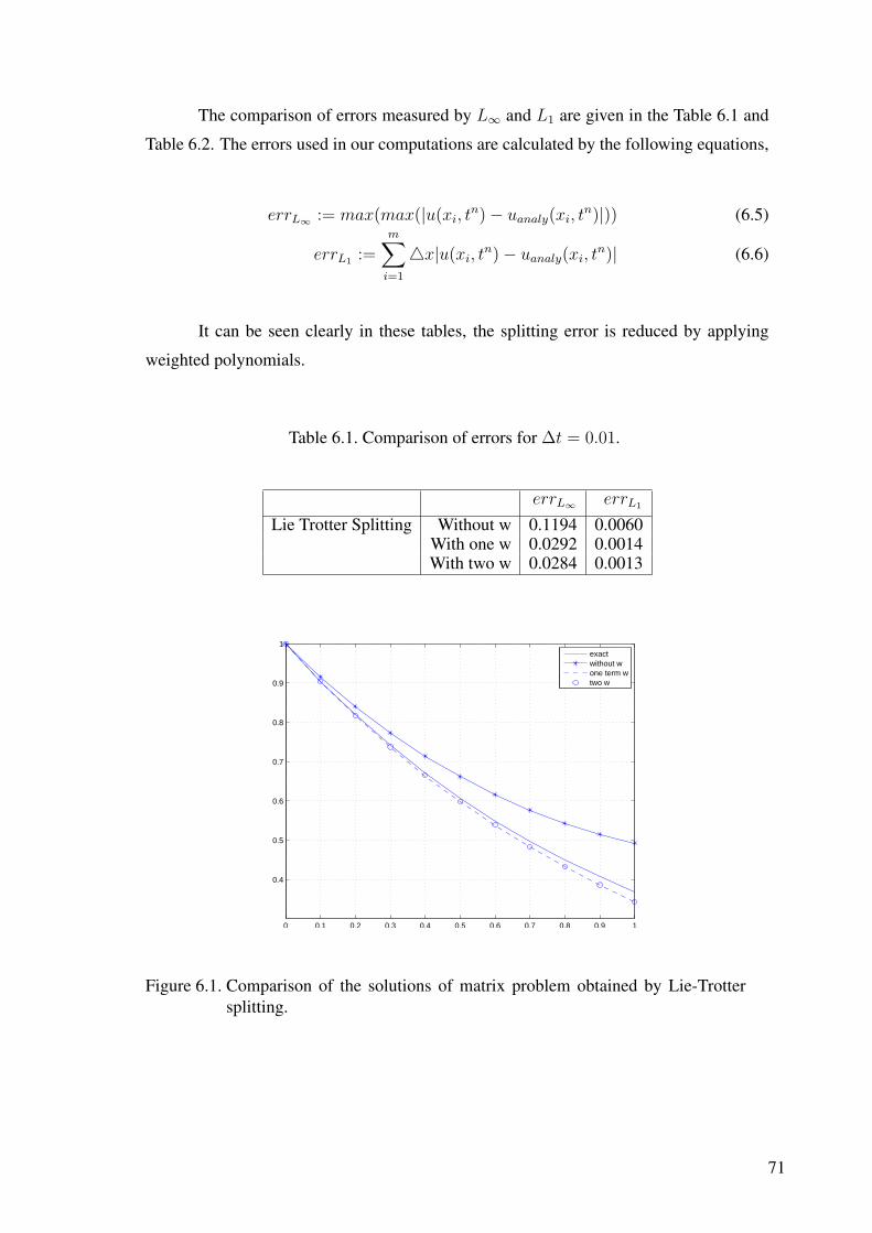
The comparison of errors measured by L∞ and L1 are given in the Table 6.1 and
Table 6.2. The errors used in our computations are calculated by the following equations,
errL∞ := max(max(|u(xi, tn)− uanaly(xi, t
n)|)) (6.5)
errL1 :=m∑
i=1
4x|u(xi, tn)− uanaly(xi, t
n)| (6.6)
It can be seen clearly in these tables, the splitting error is reduced by applying
weighted polynomials.
Table 6.1. Comparison of errors for ∆t = 0.01.
errL∞ errL1
Lie Trotter Splitting Without w 0.1194 0.0060With one w 0.0292 0.0014With two w 0.0284 0.0013
0 0.1 0.2 0.3 0.4 0.5 0.6 0.7 0.8 0.9 1
0.4
0.5
0.6
0.7
0.8
0.9
1
exactwithout wone term wtwo w
Figure 6.1. Comparison of the solutions of matrix problem obtained by Lie-Trottersplitting.
71
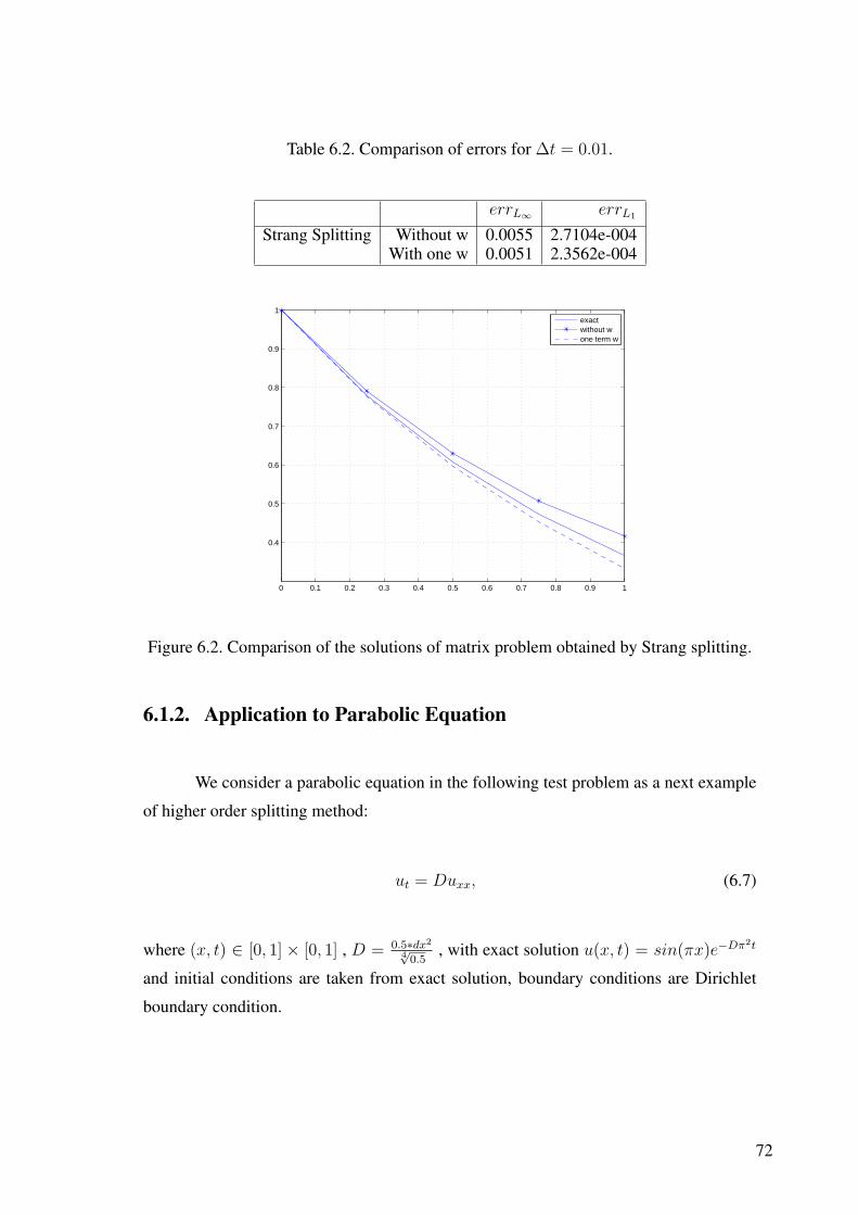
Table 6.2. Comparison of errors for ∆t = 0.01.
errL∞ errL1
Strang Splitting Without w 0.0055 2.7104e-004With one w 0.0051 2.3562e-004
0 0.1 0.2 0.3 0.4 0.5 0.6 0.7 0.8 0.9 1
0.4
0.5
0.6
0.7
0.8
0.9
1
exactwithout wone term w
Figure 6.2. Comparison of the solutions of matrix problem obtained by Strang splitting.
6.1.2. Application to Parabolic Equation
We consider a parabolic equation in the following test problem as a next example
of higher order splitting method:
ut = Duxx, (6.7)
where (x, t) ∈ [0, 1] × [0, 1] , D = 0.5∗dx2
4√0.5, with exact solution u(x, t) = sin(πx)e−Dπ2t
and initial conditions are taken from exact solution, boundary conditions are Dirichlet
boundary condition.
72
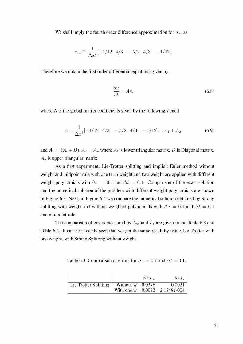
We shall imply the fourth order difference approximation for uxx as
uxx∼= 1
∆x2 [−1/12 4/3 − 5/2 4/3 − 1/12].
Therefore we obtain the first order differential equations given by
du
dt= Au, (6.8)
where A is the global matrix coefficients given by the following stencil
A =1
∆x2 [−1/12 4/3 − 5/2 4/3 − 1/12] = A1 + A2, (6.9)
and A1 = (Al + D), A2 = Au where Al is lower triangular matrix, D is Diagonal matrix,
Au is upper triangular matrix.
As a first experiment, Lie-Trotter splitting and implicit Euler method without
weight and midpoint rule with one term weight and two weight are applied with different
weight polynomials with ∆x = 0.1 and ∆t = 0.1. Comparison of the exact solution
and the numerical solution of the problem with different weight polynomials are shown
in Figure 6.3. Next, in Figure 6.4 we compare the numerical solution obtained by Strang
splitting with weight and without weighted polynomials with ∆x = 0.1 and ∆t = 0.1
and midpoint rule.
The comparison of errors measured by L∞ and L1 are given in the Table 6.3 and
Table 6.4. It can be is easily seen that we get the same result by using Lie-Trotter with
one weight, with Strang Splitting without weight.
Table 6.3. Comparison of errors for ∆x = 0.1 and ∆t = 0.1.
errL∞ errL1
Lie Trotter Splitting Without w 0.0376 0.0021With one w 0.0082 2.1848e-004
73
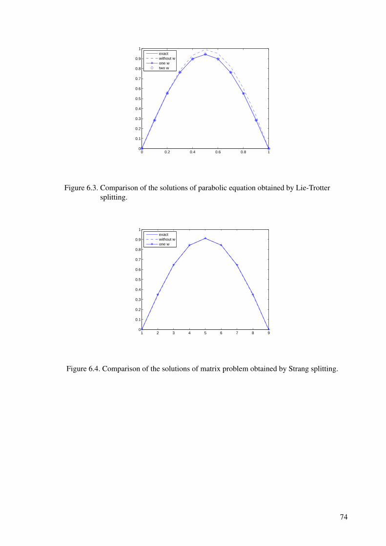
0 0.2 0.4 0.6 0.8 10
0.1
0.2
0.3
0.4
0.5
0.6
0.7
0.8
0.9
1
exactwithout wone wtwo w
Figure 6.3. Comparison of the solutions of parabolic equation obtained by Lie-Trottersplitting.
1 2 3 4 5 6 7 8 90
0.1
0.2
0.3
0.4
0.5
0.6
0.7
0.8
0.9
1
exactwithout wone w
Figure 6.4. Comparison of the solutions of matrix problem obtained by Strang splitting.
74
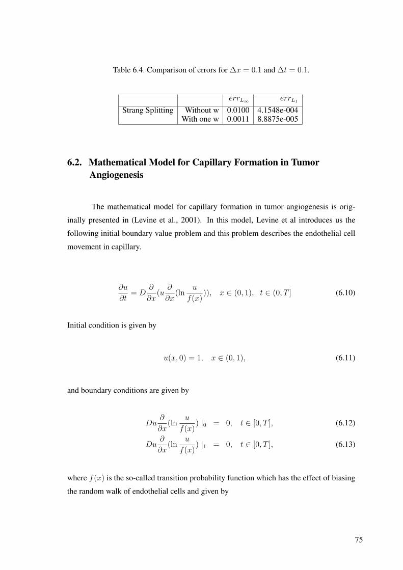
Table 6.4. Comparison of errors for ∆x = 0.1 and ∆t = 0.1.
errL∞ errL1
Strang Splitting Without w 0.0100 4.1548e-004With one w 0.0011 8.8875e-005
6.2. Mathematical Model for Capillary Formation in TumorAngiogenesis
The mathematical model for capillary formation in tumor angiogenesis is orig-
inally presented in (Levine et al., 2001). In this model, Levine et al introduces us the
following initial boundary value problem and this problem describes the endothelial cell
movement in capillary.
∂u
∂t= D
∂
∂x(u
∂
∂x(ln
u
f(x))), x ∈ (0, 1), t ∈ (0, T ] (6.10)
Initial condition is given by
u(x, 0) = 1, x ∈ (0, 1), (6.11)
and boundary conditions are given by
Du∂
∂x(ln
u
f(x)) |0 = 0, t ∈ [0, T ], (6.12)
Du∂
∂x(ln
u
f(x)) |1 = 0, t ∈ [0, T ], (6.13)
where f(x) is the so-called transition probability function which has the effect of biasing
the random walk of endothelial cells and given by
75
f(x) = (a + A1x
k(1− x)k
b + A1xk(1− x)k)α1(
c + 1− A2xk(1− x)k
d + 1− A2xk(1− x)k)α2 (6.14)
In this initial boundary value problem (6.10)-(6.13), u(x, t) is the concentration
of Endothelial Cells, D is the cell diffusion constant and a, b, c, d, A1, A2, k, α1, α2 are
some arbitrary constants.
Consider the Eq.(6.10), it can be written as
D∂
∂x(u
∂
∂x(ln
u
f(x))) = D
∂
∂x(u(
u′
u− f ′(x)
f(x))) (6.15)
and by setting F (x) = f ′(x)f(x)
we have the simplified form
ut = D(uxx − (uF (x))x). (6.16)
The initial condition is
u(x, 0) = 1, x ∈ (0, 1), (6.17)
and boundary conditions (6.12),(6.13) become
D(∂u
∂x− uF ) |0 = 0 for t > 0, (6.18)
D(∂u
∂x− uF ) |1 = 0 for t > 0, (6.19)
We split the equation
ut = D(uxx − uxF − Fxu) (6.20)
76
into two parts as follows: Diffusion part is
ut = Duxx (6.21)
and advection-reaction part is
ut = −DuxF −DFxu. (6.22)
For initial condition we have
um = 1, 0 ≤ m ≤ N, (6.23)
and for boundary conditions (6.18), (6.19), we have
D(∂u0
∂x− u0F0) = 0, for t > 0, (6.24)
D(∂uN
∂x− uNFN) = 0, for t > 0 (6.25)
where m defines the spatial discretisation step and N is the spatial discretisation number.
The derivatives terms in Eqs. (6.24), (6.25) are approximated by using the the backward
and forward difference formulas. Next, the central difference approximation for each
derivative terms uxx and ux are taken into account as follows: Diffusion term at each grid
point (xm, t) becomes
∂2u
∂x2|(xm,t)=
1
h2(um+1(t)− 2um(t) + um−1(t)) (6.26)
and advection term at each grid point (xm, t) becomes
∂u
∂x|(xm,t)=
1
2h(um+1(t)− um−1(t)) (6.27)
where h is the spatial stepping and m = 0, 1, . . . , N .
77
After assembling the unknowns of (6.26), for each m, and embedding the approxi-
mation of derivative terms in boundary conditions in (6.24), (6.25), we have the following
system of equations in matrix form as follows:
uxx = A1u (6.28)
where
A1 =1
h2
−2 + (1− hF0) 1 0 . . . 0 0
1 −2 1 . . . 0 0...
.... . . . . .
... 0
0 0 0 . . . −2 1
0 0 0 . . . 1 −2 + (1 + hFN )
(6.29)
A1 is (N + 1)× (N + 1) matrix and by assembling the unknowns of (6.27), for each m,
we obtain the following system
ux = B1u (6.30)
where
B1 =1
2h
−(1− hF0) 1 0 . . . 0 0
−1 0 1 . . . 0 0...
... . . . . . .... 0
0 0 0 . . . 0 1
0 0 0 . . . −1 (1 + hFN)
(6.31)
B1 is (N + 1)× (N + 1) matrix.
We fix the functions F (x) and F ′(x) at each discretisation points m = 0, 1, . . . , N
78

and have
F (x¯) =
F (x0) 0 . . . 0
0 F (x1) . . . 0...
... . . . ...
0 . . . 0 F (xN)
(6.32)
and
F ′(x¯) =
F ′(x0) 0 . . . 0
0 F ′(x1) . . . 0...
... . . . ...
0 . . . 0 F ′(xN)
(6.33)
where we use central difference approximation for each F ′(xm).
We finally get,
ut = (A + B)u (6.34)
where A = DA1, B = −DF (x¯)B1 −DF ′(x
¯).
For numerical computation we consider the problem (6.10)-(6.13) with parameters
D = 0.00025, a = 1, b = 2, c = 10, d = 0.1, α1 = α2 = 1, A1 = 28 × 107,
A2 = 0.22× 10⁹ and k = 16. We write the computer program in matlab and present our
results on graphs which are taken at different times.
Numerical solution of the problem (6.10)-(6.13) by using Lie-Trotter splitting,
Strang splitting and Symmetrically weighted splitting are given in Figure 6.5, Figure 6.6
and Figure 6.7.Figures show similar trends as ones that obtained by method of lines (Pa-
muk & Erdem, 2007) and exponentially-fitted method (Erdogan et al., 2009).
79
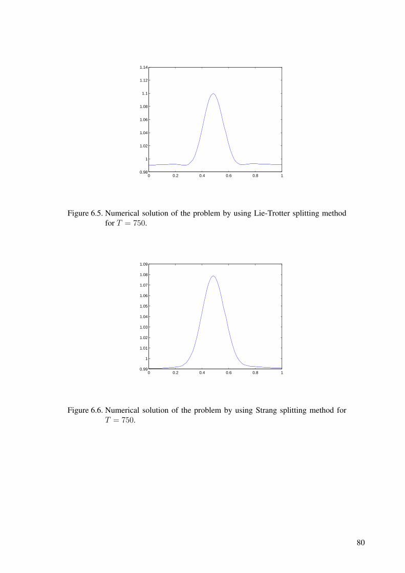
0 0.2 0.4 0.6 0.8 10.98
1
1.02
1.04
1.06
1.08
1.1
1.12
1.14
Figure 6.5. Numerical solution of the problem by using Lie-Trotter splitting methodfor T = 750.
0 0.2 0.4 0.6 0.8 10.99
1
1.01
1.02
1.03
1.04
1.05
1.06
1.07
1.08
1.09
Figure 6.6. Numerical solution of the problem by using Strang splitting method forT = 750.
80
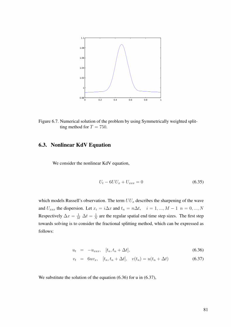
0 0.2 0.4 0.6 0.8 10.98
1
1.02
1.04
1.06
1.08
1.1
Figure 6.7. Numerical solution of the problem by using Symmetrically weighted split-ting method for T = 750.
6.3. Nonlinear KdV Equation
We consider the nonlinear KdV equation,
Ut − 6UUx + Uxxx = 0 (6.35)
which models Russell’s observation. The term UUx describes the sharpening of the wave
and Uxxx the dispersion. Let xi = i∆x and tn = n∆t, i = 1, ...,M − 1 n = 0, ..., N
Respectively ∆x = 1M
∆t = 1N
are the regular spatial end time step sizes. The first step
towards solving is to consider the fractional splitting method, which can be expressed as
follows:
ut = −uxxx, [tn, tn + ∆t], (6.36)
vt = 6uvx, [tn, tn + ∆t], v(tn) = u(tn + ∆t) (6.37)
We substitute the solution of the equation (6.36) for u in (6.37),
81
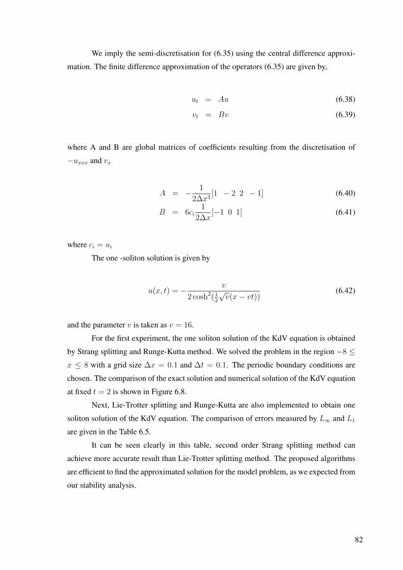
We imply the semi-discretisation for (6.35) using the central difference approxi-
mation. The finite difference approximation of the operators (6.35) are given by,
ut = Au (6.38)
vt = Bv (6.39)
where A and B are global matrices of coefficients resulting from the discretisation of
−uxxx and vx
A = − 1
2∆x3[1 − 2 2 − 1] (6.40)
B = 6ci1
2∆x[−1 0 1] (6.41)
where ci = ui
The one -soliton solution is given by
u(x, t) = − v
2 cosh2(12
√v(x− vt))
(6.42)
and the parameter v is taken as v = 16.
For the first experiment, the one soliton solution of the KdV equation is obtained
by Strang splitting and Runge-Kutta method. We solved the problem in the region −8 ≤x ≤ 8 with a grid size ∆x = 0.1 and ∆t = 0.1. The periodic boundary conditions are
chosen. The comparison of the exact solution and numerical solution of the KdV equation
at fixed t = 2 is shown in Figure 6.8.
Next, Lie-Trotter splitting and Runge-Kutta are also implemented to obtain one
soliton solution of the KdV equation. The comparison of errors measured by L∞ and L1
are given in the Table 6.5.
It can be seen clearly in this table, second order Strang splitting method can
achieve more accurate result than Lie-Trotter splitting method. The proposed algorithms
are efficient to find the approximated solution for the model problem, as we expected from
our stability analysis.
82
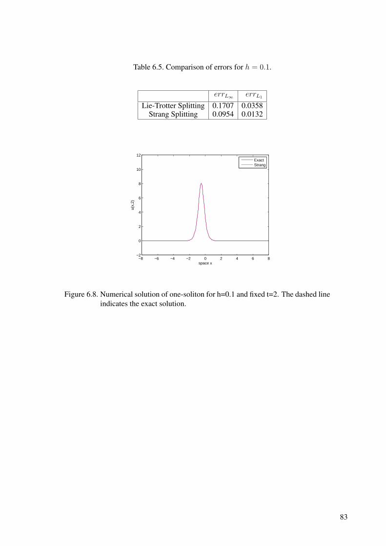
Table 6.5. Comparison of errors for h = 0.1.
errL∞ errL1
Lie-Trotter Splitting 0.1707 0.0358Strang Splitting 0.0954 0.0132
−8 −6 −4 −2 0 2 4 6 8−2
0
2
4
6
8
10
12
space x
u(x,
2)
ExactStrang
Figure 6.8. Numerical solution of one-soliton for h=0.1 and fixed t=2. The dashed lineindicates the exact solution.
83
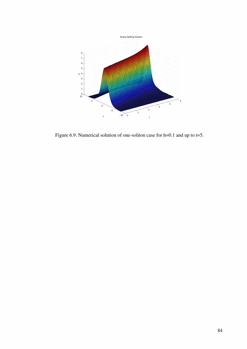
01
23
45
−10
−5
0
5
100
1
2
3
4
5
6
7
8
t
Strang Splitting Solution
x
U
Figure 6.9. Numerical solution of one-soliton case for h=0.1 and up to t=5.
84
CHAPTER 7
CONCLUSION
In this thesis, we introduced the traditional operator splitting methods; Lie-Trotter
splitting, additive splitting, symmetrically weighted splititng, Strang splitting and higher
order splitting methods which are obtained by the Zassenhaus product formula. Con-
sistency analysis for linear bounded operators are studied by the means of Zassenhaus
product formula and for unbounded operators by C0-semigroup approach. We derived
the algorithms for the nonlinear KdV equation and studied the stability analysis for these
operator splitting methods. We reformulated to Von-Neumann stability analysis for Lie-
Trotter and Strang splitting. We extend the operator splitting methods to solve various
ODEs and PDEs.
Starting with the traditional and proposed operator splitting methods are applied
to matrix problem. For that problem we observed that, the splitting error reduced by
applying weighted polynomials. We get the same result by using Lie-Trotter splitting
with one weight, with Strang splitting without weight. So, proposed operator splitting
methods lead us advantage for the CPU times.
Next, we applied the operator splitting methods to real life problem (mathematical
model for capillary formation in tumor angiogenesis). The graphs in 6.5, 6.6 and 6.7
show similar trends as the ones that obtained by method of lines and exponentially fitted
method.
Finally, we adapted the traditional splitting methods to nonlinear KdV equation.
This adaptation leads us to use Von-Neumann stability analysis for the proposed methods.
We presented the errors obtained by Lie-Trotter and Strang splitting measured by L∞ and
L1 are given in the Table 6.5. Results give us proposed algorithms work and expected
order of the accuracy for the operator splitting methods are confirmed.
85
REFERENCES
Bagrinovskii K. A. and S. K. Godunov, 1957: Difference schemes for multidimen-sional problems. Dokl. Akad. Nauk SSSR (NS), 115, 431-433.
Baker H., 1905: Alternants and Continuous Groups. Proc. London Math. Soc.,3, 24-47.
Bjorhus, M., 1988: Operator Splitting for abstract Cauchy problems. IMA Journal ofNumerical Analysis, 18, 419-443.
Blanes, S. and P.C. Moan, 2002: Practical symplectic partitioned Runge-Kutta andRunge-Kutta-Nystrom methods. J. Comp. Appl. Math., 142, 313-330.
Christov, C. I. and R. S. Marinova, 2001: Implicit vectorial operator splitting for in-compressible Navier-Stokes equations in primitive variables. J. Comput. Technol.,6, 92-119.
Crandall, M. G. and A. Majda, 1980: The method of fractional steps for conservativelaws. Math. Comp., 34, 1-21.
Csomos, P., I. Farago, & A. Havasi, 2005: Weighted sequential splittings and theiranalysis Comp. Math. Appl., 50, 1017-1031.
Daoud, Daoud S., 2007: On combination of first order Strang’s splitting and additivesplitting for the solution of the multidimensional convection diffusion problem.InternationalJournal of Computer Mathematics, 12, 1781-1794.
Dimov, I., I. Farago, A. Havasi, & Z. Zlatev, 2001: L-commutativity of the operatorsof splitting methods for air pollution models. Annales Univ. Sci. Sec. Math., 44,127-148 .
Dynkin, E. 1947: Calculation of the coefficients in Campbell-Hausdorff formula. Dokl.Akad. Nauk SSSR, 57, 323.
Engel, K.-J. & R. Nagel, 2000: One-Parameter Semigroups for Linear Evolution Equa-tions. Springer, New York.
Erdogan, U., H. Kocak, & T. Ozis, 2009: An exponentially-fitted method for solvinga mathematical model for capillary formation tumor angiogenesis problem. Com-munucation in Biomedical Engineering., to be submitted.
Farago I. and A. Havasi, 2007: Consistency analysis of operator splitting methods forC0-semigroups. Semigroup Forum., 74, 125-139.
86
Geiser, J., G. Tanoglu,& , N. Gucuyenen, 2010: Higher Order Iterative Operator-Splitting Methods for Stiff Problems: Stability Analysis and Application., NAMTA,to be submitted.
Hvistendahl Karlsen K., A. Lie , H. F. Nordhaug and H. K. Dahle 2001: Operatorsplitting methods for systems of convection-diffusion equations: Nonlinear errormechanisms and correction strategies. J. Comput. Phys., 173, 636-663.
Kahan W. and R. Li 1997: Composition constants for raising the orders of unconven-tional schemes for ordinary differential equations. Math. Comput., 66, 1089-1099.
Levine, H.A., S. Pamuk, B.D. Sleeman, 2001: Mathematical model of capillaryformation and development in tumor angiogenesis: penetration into the stroma.Bull.Math.Biol., 63, 801-863.
Magnus, W. 1954: On the exponential solution of differential equations for a linearoperator Comm. Pure Appl. Math., 7, 649.
Marchuk G. I. 1988: Methods of splitting. Nauka, Moscow.
Marinova R. S., C. I. Christov and T. T. Marinov 2003: A fully coupled solver forincompressible Navier-Stokes equations using operator splitting. Int. J. Comput.Fluid Dyn., 17, 71-385.
Mclachlan R. and R. Quispel 2002: Splitting methods. Acta Numerica, 11, 341-434.
Mimura M., T. Nakaki and K. Tomeada 1984: A numerical approach to interfacecurves for some nonlinear diffusion equations. Japan. J. Appl. Math., 1, 93-139.
Pamuk S., & A. Erdem 2007: The method of lines for the numerical solution of amathematical model for capillary formation: The roleof endothelial cells in capil-lary. Applied Mathematics and Computation., 186, 831-835.
Regan, Helen, M. 2000: Von Neumann Stability Analaysis of Symplectic IntegratorsApplied to Hamiltonian PDEs. Vol.20. 60 pp.
Scholz, D., & M. Weyrauch, 2006: A note on the Zassenhaus product formula. Journalof mathematical physics, 47, 033505.
Sheng, Q. 1993: Global error estimate for exponential splitting IMA J. Numer. Anal.,14, 27-56.
Specht W., 1948: Die linearen Beziehungen Zwischen Hoheren Kommutatoren. Math.Zeitschr., 51, 367.
Strang G., 1968: On the construction and comparison of different splitting schemes.
87
SIAM J. Numer. Anal., 5, 506-517.
Strang G., 1963: Accurate partial difference methods I: Linear Cauchy problems. Arch.Ration. Mech. Anal., 12, 392-402.
Suzuki M. 1990: Fractal decomposition of exponential operators with applications tomany-body theories and Monte Carlo simulations. Phys. Lett. A., 146, 319-323.
Verwer J. G. and B. Sportisse 1998: A note on operator splitting in a stiff linear case.CWI, Amsterdam, Netherlands, MAS-R, 9830.
Wever F., 1947: Operatoren in Leischen Ringen. J. Reine Angew. Math., 187, 44.
Yoshida H. 1990: Construction of higher order symplectic integrators. Phys. Let. A.,150, 262-268.
88
APPENDIX A
MATLAB CODES FOR THE APPLICATIONS OF THE
OPERATOR SPLITTING METHODS
HIGHER ORDER AND TRADITIONAL OPERATOR SPLITTING
METHODS MATLAB CODE FOR MATRIX PROBLEM
%Lie-Trotter splitting for matrix problem
Nt=10; A=[2 -1 ; -1 0]; B=[-2 2; 2 0];
u11=zeros(2,Nt+1); u22=zeros(2,Nt+1); u33=zeros(2,Nt+1);
u11(:,1)=[1;-1]; u22(:,1)=[1;-1]; u33(:,1)=[1;-1];
uini1=[1;-1]; uini2=[1;-1]; uini3=[1;-1];
T=1;t0=0; dt=(T-t0)/Nt
C=(B*A-A*B); D=(B*C-C*B);
E=A*(A*B-B*A)-(A*B-B*A)*A;
W1=eye(size(B))-(1/2)*C*dtˆ2;
W2=eye(size(B))-(1/2)*C*dtˆ2+((1/6)*D-(1/3)*E)*dtˆ3;
t=t0:dt:T;
for i=1:(Nt+1)
ye(i)=exp(-t(i));
end
for s=2:Nt+1,
u1=runfour(A,uini1,dt);
v1=u1;
u1=runfour(B,v1,dt);
uini1=u1;
u11(:,s)=u1;
u2=runfour(A,uini2,dt);
v2=W1*u2;
u2=runfour(B,v2,dt);
uini2=u2;
u22(:,s)=u2;
u3=runfour(A,uini3,dt);
v3=W2*u3;
89
u3=runfour(B,v3,dt);
uini3=u3;
u33(:,s)=u3;
end
u11(1,:); u22(1,:); u33(1,:)
plot(t,ye);hold on;plot(t,u11(1,:),’*-’);
hold on;plot(t,u22(1,:),’--’);
hold on;plot(t,u33(1,:),’o’);grid on;
legend(’exact’,’without w’,’one term w’,’two w’);
e1 = max(max(abs(ye-u11(1,:))))
e2=dtˆ2*sum(sum(abs(ye-u11(1,:))))
errweight1 = max(max(abs(ye-u22(1,:))))
errweight2=dtˆ2*sum(sum(abs(ye-u22(1,:))))
errweight11 = max(max(abs(ye-u33(1,:))))
errweight21=dtˆ2*sum(sum(abs(ye-u33(1,:))))
%Strang splitting for matrix problem
Nt=10;
A=[2 -1 ; -1 0];
B=[-2 2; 2 0];
u11=zeros(2,Nt+1); u22=zeros(2,Nt+1); u33=zeros(2,Nt+1);
u11(:,1)=[1;-1]; u22(:,1)=[1;-1]; u33(:,1)=[1;-1];
uini1=[1;-1]; uini2=[1;-1]; uini3=[1;-1];
T=1;t0=0; dt=(T-t0)/Nt
C=(B*A-A*B); D=(B*C-C*B);
E=A*(A*B-B*A)-(A*B-B*A)*A;
W1=eye(size(B))-((1/24)*D+(1/12)*E)*dtˆ3;
for i=1:(Nt+1)
ye(i)=exp(-t(i));
end
for s=2:Nt+1,
dtt=dt/2;
u1=runfour(A,uini1,dtt); v1=u1;
u1=runfour(B,v1,dt); v2=u1;
u1=runfour(A,v2,dtt); uini1=u1;
u11(:,s)=u1;
90
u2=runfour(A,uini2,dtt); p2=W1*u2;
u2=runfour(B,p2,dt); m2=u2;
u2=runfour(A,m2,dtt); uini2=u2;
u22(:,s)=u2;
u11(1,:); u22(1,:);
plot(t,ye);hold on;plot(t,u11(1,:),’*-’);
hold on;plot(t,u22(1,:),’--’);grid on;
legend(’exact’,’without w’,’one term w’);
function fun=runfour(A,x0,dt);
x=zeros(2,2);
x(:,1)=x0;
for i=2:2
k1=dt*fli(A,x(:,i-1));
k2=dt*fli(A,x(:,i-1)+k1/2);
k3=dt*fli(A,x(:,i-1)+k2/2);
k4=dt*fli(A,x(:,i-1)+k3);
x(:,i)= x(:,i-1)+(k1+2*k2+2*k3+k4)/6;
end fun=x(:,2);
HIGHER ORDER AND TRADITIONAL OPERATOR SPLITTING METHODS
MATLAB CODE FOR PARABOLIC PROBLEM
%%%%%% Lie-Trotter splitting for parabolic problem
xp=0;X=1;tp=0;T=1;N=10;Nt=10;
dx=1/N;dt=1/Nt;x=xp:dx:X;t=tp:dt:T;
D=(0.5*dxˆ2)/(0.5)ˆ(1/4);
k=dtˆ2;
%%%exact solution
for i=1:N
for j = 1:Nt+1
exact(i,j) = sin(pi*x(i))*exp(-D*piˆ(2)*t(j));
end end
%% initail conditon
for i = 1 : N+1
x0(i) = sin(pi*x(i))*exp(-D*piˆ(2)*t(1));
x01(i) = sin(pi*x(i))*exp(-D*piˆ(2)*t(1));
x02(i) = sin(pi*x(i))*exp(-D*piˆ(2)*t(1)); end
91
x0=x0’
sin(pi*x(N))*exp(-D*piˆ(2)*t(1));
sin(pi*x(N))*exp(-D*piˆ(2)*t(2));
sin(pi*x(N))*exp(-D*piˆ(2)*t(3));
%% boundary conditons
for j = 1 : Nt+1
xbl(j) = 0; xbr(j) = 0; end
for i=1
for j = 1:Nt+1
exact(i,j) = 0; end end
%% definition of B 4th order% -1/12 4/3 -5/2 4/3 -1/12
n=N-2; B=toeplitz([-5/2 4/3 -1/12 0 zeros(1,n-1)],
[-5/2 4/3 -1/12 0 zeros(1,n-1)]);
full(B); B = D/(dxˆ2)*B;
B(1,1)=0; B(1,2)=0; B(1,3)=0;
B(N+1,N+1)=0;B(N+1,N)=0; B(N+1,N-1)=0;
full(B);
B1=zeros(N+1,Nt+1);
B2=zeros(N+1,Nt+1);
%%%%%%%%%% B1 %%%%%%%%%%%%
n=N-2; B1=toeplitz([-5/2 0 0 0 zeros(1,n-1)],
[-5/2 4/3 -1/12 0 zeros(1,n-1)]);
full(B1); B1 = D/(dxˆ2)*B1;
B1(1,1)=0; B1(1,2)=0; B1(1,3)=0;
B1(N+1,N+1)=0;B1(N+1,N)=0; B1(N+1,N-1)=0;
full(B1);
% %%%%%%%%%%%%%%%% B2 %%%%%%%%%%%%%%%%%
n=N-2; B2=toeplitz([0 4/3 -1/12 0 zeros(1,n-1)],
[0 0 0 0 zeros(1,n-1)]);
full(B2); B2 = D/(dxˆ2)*B2;
B2(1,1)=0; B2(1,2)=0; B2(1,3)=0;
B2(N+1,N+1)=0;B2(N+1,N)=0; B2(N+1,N-1)=0;
full(B2); M=B1+B2
C=(B2*B1-B1*B2)
D=(B2*C-C*B2);
92
E=(B1*(B1*B2-B2*B1)-(B1*B2-B2*B1)*B1);
w1=eye(size(B2))-(1/2)*C*dtˆ2;
w2=eye(size(B2))-(1/2)*C*dtˆ2+((1/6)*D-(1/3)*E)*dtˆ3;
ni = [1,2,3]; for j = 1: length(ni)
ua= zeros(N+1,Nt+1,j); ua1=zeros(N+1,Nt+1,j);
ua2=zeros(N+1,Nt+1,j); end for i = 1: length(ni)
ua(:,1,i)= x0’; ua(1,:,i)= xbl(i);
ua(end,:,i)=xbr(i); ua1(:,1,i)= x0’;
ua1(1,:,i)= xbl(i); ua1(end,:,i)=xbr(i);
ua2(:,1,i)= x0’; ua2(1,:,i)= xbl(i);
ua2(end,:,i)=xbr(i); end m=1; v=2;
for a=1:Nt
erg(:,:,v) = NUM3p(B1,x0,dt,Nt,N,m,a);
v1=erg(:,a+1,v);
erg(:,:,v)=NUM3p(B2,v1,dt,Nt,N,m,a);
usp=erg(:,a+1,v);
x0=usp; ua(:,a+1,v)=usp;
erg1(:,:,v) = NUM3p(B1,x01,dt,Nt,N,v,a);
v11=w1*erg1(:,a+1,v);
erg1(:,:,v)=NUM3p(B2,v11,dt,Nt,N,v,a);
usp1=erg1(:,a+1,v);
x01=usp1; ua1(:,a+1,v)=usp1;
erg2(:,:,v) = NUM3p1(B1,x02,dt,Nt,N,v,a);
v12=w2*erg1(:,a+1,v);
erg2(:,:,v)=NUM3p1(B2,v12,dt,Nt,N,v,a);
usp2=erg2(:,a+1,v);
x02=usp2; ua2(:,a+1,v)=usp2; end
uaa=ua(:,:,v); uaa1=ua1(:,:,v); uaa2=ua1(:,:,v);
uaa(N+1,:)=0; uaa1(N+1,:)=0; uaa2(N+1,:)=0;
plot(x,exact(:,end));hold on; plot(x,uaa(:,end),’--’);
hold on; plot(x,uaa1(:,end),’-*’);
hold on;plot(x,uaa2(:,end),’o’);
legend(’exact’,’without w’,’one w’,’two w’,2);
function erg2 = NUM3p(C,x0,dt,Nt,N,k,a)
u1= zeros(N+1,Nt+1);
93
u2= zeros(N+1,Nt+1); u3= zeros(N+1,Nt+1);
u1(:,a)= x0’; u2(:,a)= x0’; u3(:,a)= x0’;
b=a+1; if k==1 for i=b:b
u1(:,i)= (eye(size(C))-dt*C) \ (u1(:,i-1));
u(1,i)= xbb; end
erg2=u1; else if k==2 for ii=b:b
C1= (eye(size(C))-(dt/2)*C);
C2= (eye(size(C))+ (dt/2)*C);
u2(:,ii)= C1 \(C2*u2(:,ii-1)); u(1,i)= xbb;
end erg2=u2; else if k==3 for ij=b:b
u11= u3(:,ij-1); a1= feval(’runge’,C,u11);
a2=feval(’runge’,C,u11+(dt/2)*a1);
a3=feval(’runge’,C,u11+(dt/2)*a2);
a4=feval(’runge’,C,u11+dt*a3);
u3(:,ij)= u3(:,ij-1)+(dt/6)*(a1+2*a2+2*a3+a4);
u(1,i)= xbb; end erg2=u3;
end end end
%%%%%% Strang splitting for parabolic problem ”
C=(B1*B2-B2*B1);
D=(B2*C-C*B2);
E=(B1*(B2*B1-B1*B2)-(B2*B1-B1*B2)*B1);
w1=eye(size(B2))+(1/24)*D*dtˆ3-(1/12)*E*dtˆ3;
v=2; m=2; for a=1:Nt
dtt=dt/2;
erg(:,:,v) = NUM3p(B1,x0,dtt,Nt,N,m,a);
v1=erg(:,a+1,v);
erg(:,:,v)=NUM3p(B2,v1,dt,Nt,N,m,a);
v2=erg(:,a+1,v)
erg(:,:,v) = NUM3p(B1,v2,dtt,Nt,N,m,a);
usp=erg(:,a+1,v);
x0=usp;
ua(:,a+1,v)=usp;
end uaa=ua(:,:,v);
uaa1=ua1(:,:,v);exact(N+1,:)=0;
uaa(N+1,:)=0;uaa1(N+1,:)=0;
94
plot(exact(:,end));hold on;
plot(uaa(:,end),’--’);hold on;
plot(uaa1(:,end),’-*’);
legend(’exact’,’without w’,’one w’,2);
e1 = max(max(abs(uaa(:,end)-exact(:,end))))
e2=dxˆ2*sum(sum(abs(uaa(:,end)-exact(:,end))))
errweight1 = max(max(abs(uaa1(:,end)-exact(:,end))))
errweight2=dxˆ2*sum(sum(abs(uaa1(:,end)-exact(:,end))))
OPERATOR SPLITTING METHODS MATLAB CODE FOR PARABOLIC
PROBLEM CAPILLARY FORMATION in TUMOR ANGIOGENESIS
%with Lie-Trotter splitting
N=64; M=50; x0=0; xl=1;
t0=0; T=500; dx=(xl-x0)/N;
dt=(T-t0)/M; D=0.00025;
r=D*dt/(dx)ˆ2;
r2=D*dt/2*dx;
x=x0:dx:xl+2*dx;
t=t0:dt:T;
% %%%%%%%% diffusion part matrix for u1’=D*A1*u1
n=N-2; A1=toeplitz([-2 1 0 0 zeros(1,n-1)],
[-2 1 0 0 zeros(1,n-1)]);
full(A1);
size(A1);
Aa=zeros(N+1);
Aa(1,1)=(1-(fu(x(2))-fu(x(1)))/fu(x(1)));
Aa(N+1,N+1)=(1+(fu(x(N+1))-fu(x(N)))/fu(x(N+1)));
A1=(A1+Aa);
A1=(1/((dx)ˆ2))*A1;
A=D*A1;
size(A);
% %%%%%%% convection part %%%%%%%
A2=toeplitz([0 -1 0 0 zeros(1,n-1)]
,[0 1 0 0 zeros(1,n-1)]);
full(A2);
Aa2=zeros(N+1);
95
Aa2(1,1)=-(1-(fu(x(2))-fu(x(1)))/fu(x(1)));
Aa2(N+1,N+1)=(1+(fu(x(N+1))-fu(x(N)))/fu(x(N+1)));
A2=D*(1/(2*dx))*(A2+Aa2);
A2;
% % %%%%%% matrixes for F(xi) %%%%%%%%%
Ff=zeros(N+1);
for i=1:N+1,
Ff(i,i)=(fu(x(i+1))-fu(x(i)))/(dx*fu(x(i)));
end Ff; Ff=D*A2*Ff;
% %%%%% matrixes for F(xi)derivative %%%%%%%%%%
Ffd=zeros(N+1);
for i=1:N+1,
Ffd(i,i)=((fu(x(i+2))-2*fu(x(i+1))+
fu(x(i)))*fu(x(i))/(dxˆ2)-((fu(x(i+1))-
fu(x(i)))ˆ2)/(dxˆ2))/(fu(x(i)))ˆ2;
end Ffd=D*Ffd;
B=-(Ff+Ffd);
% % % % % %%%%%%% initial conditions %%%
for i = 1 : N+1 x0(i) =1;
end x0=x0’;
ni = [1,2,3];
for j = 1: length(ni)
ua= zeros(N+1,M+1,j);
end for i = 1: length(ni)
ua(:,1,i)= x0’;end
m=1;v=2;
for a=1:M
erg(:,:,v) = tum(A,x0,dt,M,N,m,a);
v1=erg(:,a+1,v);
erg(:,:,v)=tum(B,v1,dt,M,N,m,a);
usp=erg(:,a+1,v);
x0=usp;
ua(:,a+1,v)=usp;
end uaa=ua(:,:,v);
s=0:dx:xl;
96
plot(s,uaa(:,end))
%% with Strang splitting
ni = [1,2,3];
for j = 1: length(ni)
ua= zeros(N+1,M+1,j);
end
for i = 1: length(ni)
ua(:,1,i)= x0’;
end m=1; v=2;
for a=1:M
dtt=dt/2;
erg(:,:,v) = tum(A,x0,dtt,M,N,m,a);
v1=erg(:,a+1,v);
erg(:,:,v)=tum(B,v1,dt,M,N,m,a);
v2=erg(:,a+1,v);
erg(:,:,v) = tum(A,v2,dtt,M,N,m,a);
usp=erg(:,a+1,v);
x0=usp;
ua(:,a+1,v)=usp;
uaa=ua(:,:,v);
s=0:dx:xl;
plot(s,uaa(:,end))
%with Symmetrically weighted splitting
ni = [1,2,3];
for j = 1: length(ni)
ua= zeros(N+1,M+1,j);
ua1= zeros(N+1,M+1,j);
end
for i = 1: length(ni)
ua(:,1,i)= x0’;
ua1(:,1,i)= x01’;
end m=1; v=2;
for a=1:M
erg(:,:,v) = tum(A,x0,dt,M,N,m,a);
v1=erg(:,a+1,v);
97
erg(:,:,v)=tum(B,v1,dt,M,N,m,a);
usp=erg(:,a+1,v);
x0=usp;
ua(:,a+1,v)=usp;
erg2(:,:,v) = tum(B,x01,dt,M,N,m,a);
v2=erg(:,a+1,v);
erg2(:,:,v)=tum(A,v2,dt,M,N,m,a);
usp1=erg2(:,a+1,v)
x01=usp1;
ua1(:,a+1,v)=usp1;
end
uaa=ua(:,:,v);
uaa1=ua1(:,:,v);
uaaa=(uaa+uaa1)/2;
s=0:dx:xl;
plot(s,uaaa(:,end))
function erg2 = tum(C,x0,dt,M,N,k,a)
u1= zeros(N+1,M+1);
u2= zeros(N+1,M+1);
u3= zeros(N+1,M+1);
u1(:,a)= x0’;u2(:,a)= x0’;
u3(:,a)= x0’; b=a+1;
if k==1 for i=b:b
u1(:,i)= (eye(size(C))-dt*C)\(u1(:,i-1));
end erg2=u1;
else if k==2
for ii=b:b
C1= (eye(size(C))-(dt/2)*C);
C2= (eye(size(C))+ (dt/2)*C);
u2(:,ii)= C1 \(C2*u2(:,ii-1));
end erg2=u2;
else if k==3
for ij=b:b
u11= u3(:,ij-1);
a1= feval(’runge’,C,u11);
98
a2=feval(’runge’,C,u11+(dt/2)*a1);
a3=feval(’runge’,C,u11+(dt/2)*a2);
a4=feval(’runge’,C,u11+dt*a3);
u3(:,ij)= u3(:,ij-1)+(dt/6)*(a1+2*a2+2*a3+a4);
end erg2=u3;
end end end
SPLITTING METHODS MATLAB CODE FOR NONLINEAR KdV
%%Soliton with Lie-Trotter
function solitona
h=0.1;
x=(-8+h:h:8)’;
m=length(x);
k=hˆ3;
n=2/k;
u=firstsol(x,16,0);
for i=1:n
a11=k*f1(u); a21=k*f1(u+a11/2);
a31=k*f1(u+a21/2); a41=k*f1(u+a31);
u=u+a11/6+a21/3+a31/3+a41/6;
a1=k*f2(u); a2=k*f2(u+a1/2);
a3=k*f2(u+a2/2); a4=k*f2(u+a3);
u=u+a1/6+a2/3+a3/3+a4/6;
end
plot(x,-u);
axis([-8,8,-2,12])
xlabel(’space x’)
ylabel(’u(x,2)’)
function dudt=f1(u)
u = [u(end-1:end); u; u(1:2)]; h=.1;
dudt = -(u(5:end)-2*u(4:end-1)+
2*u(2:end-3)-u(1:end-4))/2/hˆ3;
function dudt=f2(u)
u = [u(end-1:end); u; u(1:2)]; h=.1;
dudt = 6*(u(3:end-2)).*(u(4:end-1)
-u(2:end-3))/2/h;
99
function u=firstsol(x,v,x0)
u=-v/2./cosh(.5*sqrt(v)*(x-x0)).ˆ2;
%%% Soliton wiith strang Splitting
function solitonst
a11=s*f1(u); a21=s*f1(u+a11/2);
a31=s*f1(u+a21/2); a41=s*f1(u+a31);
u=u+a11/6+a21/3+a31/3+a41/6;
a1=k*f2(u); a2=k*f2(u+a1/2);
a3=k*f2(u+a2/2); a4=k*f2(u+a3);
u=u+a1/6+a2/3+a3/3+a4/6;
a12=s*f1(u); a22=s*f1(u+a12/2);
a32=s*f1(u+a22/2); a42=s*f1(u+a32);
u=u+a12/6+a22/3+a32/3+a42/6;
end
plot(x,-u1); hold on;
plot(x,-u,’r’);
axis([-8,8,-2,12])
xlabel(’space x’)
ylabel(’u(x,2)’)
100


![Operator Splitting Methods for Approximating Differential Equations€¦ · 1 2 [exp(tA)exp(tB) + exp(tB)exp(tA)]u0 + O(t3) Joshua Lee Padgett Texas Tech University February 27, 2018](https://img.pdfslide.us/doc/110x75/5f970478d44bc474551ae33f/operator-splitting-methods-for-approximating-differential-equations-1-2-exptaexptb.jpg)