Operator splitting - UCLAwotaoyin/splittingbook/ch3-macnamara-strang.pdf · Operator splitting Shev MacNamara and Gilbert Strang Abstract Operator splitting is a numerical method

Operator splitting

Shev MacNamara and Gilbert Strang

Abstract Operator splitting is a numerical method of computing the solution to adifferential equation. The splitting method separates the original equation into twoparts over a time step, separately computes the solution to each part, and then com-bines the two separate solutions to form a solution to the original equation. A canon-ical example is splitting of diffusion terms and convection terms in a convection-diffusion partial differential equation. Related applications of splitting for reaction-diffusion partial differential equations in chemistry and in biology are emphasizedhere. The splitting idea generalizes in a natural way to equations with more than twooperators. In all cases, the computational advantage is that it is faster to compute thesolution of the split terms separately, than to compute the solution directly whenthey are treated together. However, this comes at the cost of an error introducedby the splitting, so strategies have been devised to control this error. This chapterintroduces splitting methods and surveys recent developments in the area. An in-teresting perspective on absorbing boundary conditions in wave equations comesvia Toeplitz-plus-Hankel splitting. One recent development, balanced splitting, de-serves and receives special mention: it is a new splitting method that correctly cap-tures steady state behavior.

1 Introduction

It has been said that there are only ten big ideas in numerical analysis; all the restare merely variations on those themes. One example of those big ideas is multi-scale computational approaches. A multi-scale motif reappears in numerous places

Shev MacNamaraSchool of Mathematics, University of New South Wales, Sydney NSW 2052, Australia. e-mail:[email protected]

Gilbert StrangDepartment of Mathematics, MIT, Cambridge, MA, 02139. e-mail: [email protected]

1

2 Shev MacNamara and Gilbert Strang

including: multigrid for solving linear systems [51], wavelets for image processing[11], and in Multi-level Monte Carlo for the solution of stochastic differential equa-tions [20]. Another of those big ideas could surely be splitting [42, 4, 57]: start witha complicated problem, split it into simpler constituent parts that can each be solvedseparately, and combine those separate solutions in a controlled way to solve theoriginal overall problem. Often we solve the separate parts sequentially. The outputof the first subproblem is the input to the next subproblem (within the time step).

Like all great ideas, splitting is a theme that continues to resurface in manyplaces. Splitting principles have taken a number of generic forms:

• Split linear from nonlinear.• Split x-direction from y-direction (dimensional splitting).• Split terms corresponding to different physical processes. For example, split con-

vection from diffusion in ODEs or in PDEs.• Split a large domain into smaller pieces. For example, domain decomposition

helps to solve large PDEs in parallel.• Split objective functions in optimization.• Split resolvents when solving linear systems: Instead of working directly with

(λ III − (AAA+BBB))−1, we iterate between working separately with each of (λ III −AAA)−1 and (λ III−BBB)−1.

Not surprisingly, a principle as fundamental as splitting finds applications inmany areas. Here is a non-exhaustive list:

• A recent application of splitting is to low-rank approximation [36].• Balanced splitting has been developed to preserve the steady state [53].• Splitting of reaction terms from diffusion terms in reaction-diffusion PDEs is

a common application of splitting in biology. Now splitting is also finding ap-plications in stochastic, particle-based methods, such as for master equations[19, 32, 38, 37, 18, 26, 25], including analysis of sample path approaches [16].

• Splitting stochastic differential equations, by applying the component operatorsin a random sequence determined by coin flipping is, on average, accurate. Thishas applications in finance [45]. Though in a different sense, splitting also findsapplication in Monte Carlo estimation of expectations [2].

• Maxwell’s equations for electromagnetic waves can be solved on staggered gridsvia Yee’s method, which is closely related to splitting [55, 34].

• Motivated in part by the need for accurate oil reservoir simulations, AlternatingDirection Implicit methods and Douglas-Rachford splittings have by now foundwide applications [62, 47, 14].

• Split-Bregman methods are a success for compressed sensing and for image pro-cessing [21].

• Navier-Stokes equations in fluid mechanics are often approximated numeri-cally by splitting the equations into three parts: (i) a nonlinear convection term,u · (∇u), is treated explicitly, (ii) diffusion, ∆u, is treated implicitly, and (iii) con-tinuity is imposed via Poisson’s equation, divu = 0 . Chorin’s splitting method isa well-known example of this approach [7, 55].

Operator splitting 3

• Split the problem of finding a point in the intersection of two or more sets intoalternating projections onto the individual sets [4].

This chapter places emphasis on applications to partial differential equations(PDEs) involving reaction, diffusion and convection. Balanced splitting, which hasfound application in models of combustion, receives special attention. Computersimulation of combustion is important to understand how efficiently or how cleanlyfuels burn. It is common to use operator splitting to solve the model equations.However, in practice this was observed to lead to an unacceptable error at steadystate. The new method of balanced splitting was developed to correct this [53]. Thisbalanced method might be more widely applicable because operator splitting is usedin many areas. Often the steady state is important. In reaction-diffusion models, inbiology for example, it is very common to split reaction terms from diffusion terms,and the steady state is almost always of interest. As we will see in the next section,the most obvious splitting scheme is only first order accurate but a symmetrizedversion achieves second order accuracy. Do such schemes yield the correct steadystate? The answer is no, not usually. Balanced splitting corrects this.

Outline: The rest of this chapter is organized as follows. We begin with the sim-plest possible example of splitting. First order accurate and second order accuratesplitting methods come naturally. Higher order splitting methods, and reasons whythey are not always adopted, are then discussed. Next, we observe that splittingdoes not capture the correct steady state. This motivates the introduction of bal-anced splitting: a new splitting method that does preserve the steady state. All theseideas are illustrated by examples drawn from reaction-diffusion PDEs such as arisein mathematical biology, and from convection-diffusion-reaction PDEs such as inmodels of combustion. We aim especially to bring out some recent developmentsin these areas [59, 53]. Finally, we investigate a very special Toeplitz-plus-Hankelsplitting, that sheds light on the reflections at the boundary in a wave equation.

2 Splitting for ordinary differential equations

The best example to start with is the linear ordinary differential equation (ODE)

dudt

= (AAA+BBB)u. (1)

The solution is well known to students of undergraduate differential equationcourses [58]:

u(h) = eh(AAA+BBB)u(0),

at time h. We are interested in splitting methods that will compute that solution forus, at least approximately. If we could simply directly compute eh(AAA+BBB), then wewould have solved our ODE (1), and we would have no need for a splitting approx-imation. However, in applications it often happens that eh(AAA+BBB) is relatively difficultto compute directly, whilst there are readily available methods to compute each of


ehAAA and ehBBB separately. For example, (1) may arise as a method-of-lines approxima-tion to a PDE in which AAA is a finite difference approximation to diffusion, and BBBis a finite difference approximation to convection. (This example of an convection-diffusion PDE, together with explicit matrices, is coming next.) In that case it isnatural to make the approximation

First order splitting eh(AAA+BBB) ≈ ehAAAehBBB. (2)

We call this approximate method of computing the solution splitting. This chapterstays with examples where AAA and BBB are matrices, although the same ideas apply inmore general settings where AAA and BBB are operators; hence the common terminologyoperator splitting.

To begin thinking about a splitting method we need to see the matrix that appearsin the ODE as the sum of two matrices. That sum is immediately obvious in (1) bythe way it was deliberately written. However, had we instead been given the ODEdu/dt = MMMu, then before we could apply a splitting method, we would first needto identify AAA and BBB that add up to MMM. Given MMM, identifying a good choice for AAAand thus for BBB = MMM−AAA is not trivial, and the choice is critical for good splittingapproximations.

When the matrices commute, the approximation is exact. 1 That is, if the commu-tator [AAA,BBB]≡ AAABBB−BBBAAA = 000, then eh(AAA+BBB) = ehAAAehBBB. Otherwise the approximation of(2), eh(AAA+BBB) ≈ ehAAAehBBB, is only first order accurate: the Taylor series of ehAAAehBBB agreeswith the Taylor series of eh(AAA+BBB) up to first order, but the second order terms differ.The Taylor series is

eh(AAA+BBB) = III +h(AAA+BBB)+12

h2(AAA+BBB)2 + . . .

If we expand (AAA+BBB)2 = AAA2 +AAABBB+BBBAAA+BBB2 then we see the reason we are lim-ited to first order accuracy. In all terms in the Taylor series for our simple splittingapproximation ehAAAehBBB, AAA always comes before BBB, so we can not match the term BBBAAAappearing in the correct series for eh(AAA+BBB).

The previous observation suggests that symmetry might help and indeed it does.The symmetric Strang splitting [54, 57]

Second order splitting eh(AAA+BBB) ≈ e12 hAAAehBBBe

12 hAAA

(3)

1 An exercise in Golub and Van Loan [22] shows that [AAA,BBB] = 000 if and only if eh(AAA+BBB) = ehAAAehBBB

for all h.


agrees with this Taylor series up to second order so it is a more accurate approx-imation than (2). Splitting methods have grown to have a rich history with manywonderful contributors. Marchuk is another of the important pioneers in the field.He found independently the second-order accurate splitting that we develop andextend in this chapter [40, 41].

When we numerically solve the ODE (1) on a time interval [0 T ], we usually donot compute u(T ) = eT (AAA+BBB)u(0) in one big step time step T , nor do we approximateit by e

12 T AAAeT BBBe

12 T AAAu(0). Our approximations are accurate for small time steps h > 0

but not for large times T . Therefore, instead, we take very many small steps h thatadd up to T . The first step is v1 = e

12 hAAAehBBBe

12 hAAA u(0), which is our approximation

to the solution of (1) at time h. The next step is computed from the previous step,recursively, by vi+1 = e

12 hAAAehBBBe

12 hAAA vi, so that vi is our approximation to the exact

solution u(ih) at time ih for i = 1,2, . . . . After N steps, so that Nh = T , we arrive atthe desired approximation vN ≈ u(T ).

Notice that a few Strang steps in succession

(e12 hAAAehBBBe

12 hAAA) (e

12 hAAAehBBBe

12 hAAA) = (e

12 hAAAehBBB) ehAAAehBBB︸︷︷︸

first order step

(e12 hAAA)

is the same as a first order step in the middle, with a special half-step at the start anda different half-step at the end. This observation helps to reduce the overall workrequired to achieve second order accuracy when taking many steps in a row. Thiswas noticed in the original paper [54] but perhaps it is not exploited as often as itcould be.

Here is a more explicit example of first order and of second order accuracy. No-tice the difference between the local error over one small time step h, and the globalerror over the whole time interval (those local errors grow or decay). We are inter-ested in how fast the error decays as the time step h becomes smaller. The power ofh is the key number. In general, the local error is one power of h more accurate thanthe global error from 1/h steps. Comparing Taylor series shows that

local error e12 hAAAehBBBe

12 hAAA− eh(AAA+BBB) =CCCh3 +O(h4).

where the constant is CCC = 124 ([[AAA,BBB],AAA] + 2[[AAA,BBB],BBB]). That is, for a single small

time step h, the symmetric Strang splitting (3) has a local error that decays like h3.As usual, the error gets smaller as we reduce the time step h: if we reduce the timestep h from 1 to 0.1, then we expect the error to reduce by a factor of 0.13 = 0.001.However, to compute the solution at the final time T , we take T/h steps, thus moresteps with smaller h, and the global error is (number of steps)× (error at each step)= (1/h)h3 = h2, so we say the method is second order accurate.

We have examined accuracy by directly comparing the Taylor series of the exactsolution and of the approximation. Another approach is via the Baker-Campbell-Hausdorff (BCH) formula:


CCC(hAAA,hBBB) = hAAA+hBBB+12[hAAA,hBBB]+ · · · ,

which, given AAA and BBB, is an infinite series for the matrix CCC such that eCCC = ehAAAehBBB. Innonlinear problems we want approximations that are symplectic. Then area in phasespace is conserved, and approximate solutions to nearby problems remain close. Thebeautiful book of Hairer, Lubich and Wanner [24] discusses the BCH formula andits connection to splitting, and when splitting methods are symplectic for nonlinearequations. Strang splitting is symplectic.

2.1 Gaining an order of accuracy by taking an average

The nonsymmetric splitting eh(AAA+BBB) ≈ ehAAAehBBB is only first order accurate. Of course,applying the operations the other way around, as in ehBBBehAAA is still only first order ac-curate. However, taking the average of these two first order approximations recoversa certain satisfying symmetry

eh(AAA+BBB) ≈ ehAAAehBBB + ehBBBehAAA

2.

Symmetry is often associated with higher order methods. Indeed this symmetric av-erage is second order accurate. That is, we gain one order of accuracy by taking anaverage. Whilst this observation is for averages in a very simple setting, we con-jecture that it is closely related to the good experience reported in the setting offinance, where a stochastic differential equation is solved with good accuracy in theweak sense even if the order of operations is randomly determined by ‘coin flipping’[45].

2.2 Higher order methods

Naturally, we wonder about achieving higher accuracy with splitting methods. Per-haps third-order splitting schemes or even higher order splitting schemes, are pos-sible. Indeed they are, at least in theory. However, they are more complicated toimplement: third order or higher order splitting schemes require either substeps thatgo backwards in time or forward in ‘complex time’ [3, 65, 24, 34, 13, 12]. For diffu-sion equations, going backwards in time raises serious issues of numerical stability.For reaction-diffusion equations, second-order splitting is still the most popular.

More generally, it is a meta-theorem of numerical analysis that second ordermethods often achieve the right balance between accuracy and complexity. Firstorder methods are not accurate enough. Third order and higher order methods areaccurate, but they have their own problems associated with stability or with being


too complicated to implement. Dahlquist and Henrici were amongst the pioneers touncover these themes [5, 9, 10, 31].

2.3 Convection and diffusion

Until now, the discussion has been concerned with ODEs: time but no space. How-ever, a big application of splitting is to PDEs: space and time.

An example is a PDE in one space dimension that models convection and dif-fusion. The continuous, exact solution u(x, t) is to be approximated by finite dif-ferences. We compute a discrete approximation on a regular grid in space x =. . . ,−2∆x,−∆x,0,∆x,2∆x, . . . One part of our PDE is convection du/dt = du/dx.Convection is often represented by a one-sided finite difference matrix. For exam-ple, the finite difference approximation du/dx ≈ (u(x+∆x)−u(x))/∆x comes viathe matrix

PPP =1

∆x

-1 1-1 1

. . . . . .

.Or we can approximate convection by a centered difference matrix:

QQQ =1

2∆x

0 1-1 0 1

. . . . . . . . .

.Here we think of du/dx≈ (u(x+h)−u(x−h))/2∆x≈QQQu. Another part of our PDEis diffusion: du/dt = d2u/dx2. The second spatial difference is often represented bythe matrix

DDD =1

∆x2

-2 11 -2 1

. . . . . . . . .

.We will come back to this matrix at the end of the chapter in (8), where we changesigns to KKK =−DDD so that KKK is positive definite and KKK models −d2/dx2. In solving asimple linear PDE with convection and diffusion terms

∂u∂ t

=∂u∂x︸︷︷︸

convection

+∂ 2u∂x2︸︷︷︸

diffusion

with finite differences we may thus arrive at the ODE

dudt

= (PPP+DDD)u. (4)


Here in the ODE we think of u(t) as a column vector, with components storingthe values of the solution on the spatial grid [. . . ,u(−∆x),u(0),u(∆x), . . . ]T . (Weare abusing notation slightly by using the same u in the PDE and in its ODE ap-proximation.) This is a discrete-in-space and continuous-in-time, or semi-discreteapproximation. We recognize it as the same ODE that we introduced at the verybeginning (1), here with the particular choice AAA = DDD and BBB = PPP. The solution tothis semi-discrete approximation is the same u(t) = eh(PPP+DDD)u(0), and it is naturalto consider approximating this solution by splitting into convection PPP and diffusionterms DDD.

In applying the splitting method (2), we somehow compute the approximationehPPPehDDDu(0). Conceivably, we might choose to compute each of the matrix exponen-tials, ehPPP and ehDDD, in full, and then multiply these full matrices by the vector u(0).In practice that is usually not a good idea. One reason is that the matrices are of-ten sparse, as in the examples of DDD and PPP here, and we want to take advantage ofthat sparsity, whereas the matrix exponential is typically full. Moreover, comput-ing the matrix exponential is a classical problem of numerical analysis with manychallenges [43].

Usually we only want the solution vector u(t), not a whole matrix. For this pur-pose, ODE-solvers, such as Runge-Kutta methods or Adams-Bashforth methods,are a good choice [5, 31]. The point of this chapter is merely to observe that we canstill apply splitting methods. We proceed in two stages. First stage: starting fromu(0), solve du/dt = DDDu from time t = 0 to t = h for the solution w1/2. Second stage:starting from this w1/2, solve du/dt = PPPu from time t = 0 to t = h for the solu-tion w2/2. Thus we have carried out a first order splitting: if our ODE-solvers wereexact at each of the two stages, then w2/2 = ehAAAehBBBu(0). Often, we treat the dif-fusion term implicitly [1]. Hundsdorfer and Verwer discuss the numerical solutionof convection-diffusion-reaction problems, noting additional issues when applyingsplitting methods to boundary value problems [30].

2.4 A reaction-diffusion PDE: splitting linear from nonlinear

A typical example in mathematical biology is a reaction-diffusion PDE in the form

∂

∂ t

[uv

]=

(∇ ···[

Du 00 Dv

]∇

)︸︷︷︸

diffusion

[uv

]+

[f (u,v)g(u,v)

]︸︷︷︸

reaction

. (5)

Here Du and Dv are positive diffusion constants for the concentrations of the twospecies u and v, respectively. Commonly these are modeled as genuinely constant –not spatially varying – and in the special case that Du = Dv = 1, then our diffusionoperator simplifies to ∇ ···∇, which many authors would denote by ∇2, or in onespace dimension by ∂ 2/∂x2. The reactions are modeled by nonlinear functions f


and g . For example, in a Gierer-Meinhardt model, f (u,v) = a− bu+ u2/v2, andg(u,v) = u2− v [44, 39].

Diffusion is linear. Reactions are nonlinear. We split these two terms and solvethem separately. We solve the linear diffusion implicitly. The nonlinear reactions aresolved explicitly. By analysis of our linear test problem (1) we found the accuracyof splitting approximations to be second order accurate, in the case of symmet-ric Strang splitting. However, the questions of accuracy and of stability concerningsplitting approximations to the more general form

dudt

= AAAu+ f (u)

where AAA is still linear but now f is nonlinear, such as arise in reaction-diffusionPDEs, has no such simple answer [52, 1].

2.5 Stability of splitting methods

We have seen that splitting can be accurate. Now we wonder about stability. To-gether, stability and consistency imply convergence. That is both a real theorem formany fundamental examples, and also a meta-theorem of numerical analysis [33].Indeed it is sometimes suggested (together with its converse) as The FundamentalTheorem of Numerical Analysis [60, 63, 8, 55].

In this context those three keywords have special meanings. Accuracy meansthat the computed approximation is close to the exact solution. A method is stableif over many steps, the local errors only grow slowly in a controlled way and donot come to dominate the solution. (A mathematical problem is well-conditioned ifsmall perturbations in the input only result in correspondingly small perturbations inthe output. Stability for numerical algorithms is analogous to the idea of condition-ing for mathematical problems.) The method is consistent if, over a single time steph, the numerical approximation is more and more accurate as h becomes smaller. Forinstance, we saw that the local error of a single step with symmetric Strang splitting(3), scales like h3 as h→ 0, so that method is consistent. For a consistent method,we hope that the global error, after many time steps, also goes to zero as h→ 0:if this happens then the numerical approximation is converging to the true solution.Usually, finding a direct proof of convergence is a formidable task, whereas showingconsistency and showing stability separately is more attainable. Then the theoremprovides the desired assurance of convergence.

When we start thinking about the question of stability of splitting methods, typi-cally we assume that the eigenvalues of AAA and of BBB all lie in the left half, Re(λ )≤ 0,of the complex plane. Separately, each system is assumed stable.

It is natural to wonder if the eigenvalues of (AAA+BBB) also lie in the left half plane.This is not true in general. Turing patterns2 in mathematical biology are a famous

2 See, for example, Rauch’s notes on Turing instability [48].


instance of this [44, 39]. Typically we linearise at a steady state. For example, if JJJ isthe Jacobian matrix of the reaction terms in (5) at the steady state, then we study thelinear equation duuu/dt = (JJJ+DDD)uuu, where uuu = [u v]T . Separately, the diffusion oper-ator DDD, and the Jacobian JJJ each have eigenvalues with negative real part. Analysisof Turing instability begins by identifying conditions under which an eigenvalue of(JJJ+DDD) can still have a positive real part.

With the assumption that all eigenvalues of MMM have negative real part, etMMM isstable for large times t. If the matrix MMM is real symmetric then the matrix exponentialehMMM is also well behaved for small times. Otherwise, whilst eigenvalues do governthe long-time behavior of etMMM , the transient behavior can be different if there isa significant pseudospectrum [61]. This can happen when the eigenvectors of thematrix are not orthogonal, and the convection-diffusion operator is an importantexample [49].

Even if the matrix exponentials et(AAA+BBB), etAAA, and etBBB are stable separately, wedon’t yet know about the stability of their multiplicative combination, as in say, firstorder splitting, ehAAAehBBB. A sufficient condition for stability is that the symmetric parts

symmetric part AAAsym ≡AAA+AAAT

2

of AAA and of BBB are negative definite. In that case we have stability of both ordinarysplitting and symmetric Strang splitting because separately ||ehAAA|| ≤ 1 and ||ehBBB|| ≤1. This result was proved by Dahlquist and the idea is closely related to the lognorm of a matrix. One way to show this is to observe that the derivative of ||ehAAAu||2is ((AAA+AAAT )ehAAAu,ehAAAu) ≤ 0. Another way is to let AAA = AAAsym +AAAanti, and observethat ehAAA is the limit of ehAAAsym/nehAAAanti/nehAAAsym/n . . .ehAAAanti/n. Each ||ehAAAsym/n|| ≤ 1 sinceeigenvalues of AAAsym are negative and the matrix is symmetric. Each ||ehAAAanti/n|| ≤ 1since eigenvalues of ehAAAanti/n are purely imaginary and the matrix is orthogonal.

Returning to the convection-diffusion example (4), we can now see that the split-ting method is stable. In that case, note that PPP = QQQ+ hDDD, where QQQ is the antisym-metric part and hDDD is the symmetric part. Observing that the diffusion matrix DDDis symmetric negative definite, we see that such a splitting is strongly stable withsymmetric Strang splitting.

Having established that splitting is stable and accurate over finite times, we havenow investigated many of the concerns of the original paper on Strang splitting:

Surprisingly, there seem to be no recognized rules for thecomparison of alternative difference schemes. Clearly thereare three fundamental criteria -- accuracy, simplicity, andstability -- and we shall evaluate each of the competingschemes in these terms.

– “ On the Construction and Comparison of Difference Schemes”Gilbert Strang, SIAM J. Numer. Anal., 1968.

Perhaps another criterion could have been added – how well the method transi-tions from an early transient behavior to late stage steady state behavior. It turns out


that most splitting schemes do not exactly capture the all-important steady state. Wereview next a new “balanced splitting” scheme that corrects this error.

2.6 Ordinary splitting does NOT preserve the steady state

Suppose u∞ is a steady state of (1). By definition

(AAA+BBB)u∞ = 0 and eAAA+BBBu∞ = u∞.

In special cases, such as when AAAu∞ = BBBu∞ = 0, both first order splitting (2), andsecond order splitting (3) preserve steady states of the original ODE. However,in general, standard splitting approximations do not preserve the steady state u∞:ehAAAehBBBu∞ 6= u∞ and e

12 hAAAehBBBe

12 hAAAu∞ 6= u∞.

3 Balanced splitting: a symmetric Strang splitting that preservesthe steady state

We again consider our linear ODE dv/dt = (AAA+BBB)v. In balanced splitting [53]a constant vector, c, is computed at the beginning of each step. Then c is added toAAAv and subtracted from BBBv in the substages of the splitting approximation; the partsstill add to (AAA+BBB)v.

A first idea (simple balancing) is to choose c so that AAAv+ c = BBBv− c. Then thefirst stage solves

dv/dt = AAAv+ c, c =12(BBB−AAA)v0, v0 = u0, (6)

for the solution3 v+ = ehAAAv0 + (ehAAA − III)AAA−1c, at time h . Now the second stagesolves

dv/dt = BBBv− c, v0 = v+,

for the solution ehBBBv+− (ehBBB− III)BBB−1c at time h. We call this method ‘nonsymmet-ric balanced splitting’. By adding and subtracting a constant vector, we see this asa modification of first order splitting (2), but the modified version has an advan-tage near steady state. Actually this choice of c = 1

2 (BBB−AAA)v frequently leads toinstability [53].

Of course there is also a simple modification of the second order splitting (3)approximation, where we add and subtract a constant at each stage. In symmetricbalanced splitting, we solve the ‘AAA stage’ for a time step 1

2 h, then the ‘BBB stage’

3 Here we assume AAA and BBB are invertible. The non-invertible case is treated by the variation-of-parameters formula [58].


for a time step h, and finally the ‘AAA stage’ again for a time step 12 h. That is, in the

‘symmetric balanced splitting method’, the first stage { dv/dt = AAAv+c, v0 = u0 }, isthe same as before except that we solve for the solution over a smaller interval h/2.Then v+ = e

12 hAAAv0+(e

12 hAAA−III)AAA−1c, is the initial condition for the second stage. We

solve for v++ over the time interval h. The third stage is { dv/dt =AAAv+c, v0 = v++ }over the remaining half step h/2. The output, v(h) = RRRv(0), is the approximation atthe end of the whole step, where

RRR =12

(III−AAA−1BBB+ e

12 hAAAehBBBe

12 hAAA(III +AAA−1BBB)

+e12 hAAA(ehBBB− III)(BBB−1AAA−AAA−1BBB)

). (7)

In the special case that AAA = BBB, the formula simplifies to RRR = e12 hAAAehBBBe

12 hAAA so

symmetric balanced splitting is identical with symmetric Strang splitting in thiscase. This is what we expect because in this case c = 0. To improve stabilitywe may choose different balancing constants, thereby moving from simple bal-anced splitting to rebalanced splitting [53]. One good choice [53, equation 7.7]is cn+1 = (−vn+1 + 2v++

n − 2v+n + vn)/2h+ cn, which involves all values from theprevious step.

3.1 Balanced splitting preserves the steady state

Having introduced the method of balanced splitting, we now confirm its most im-portant property. Recall that we are at a steady state if and only if the derivative iszero. Hence we may check that a steady state, u∞, of the original system (1). is alsoa steady state of the new balanced splitting approximation by direct substitution andevaluation of the derivative. Suppose that we start at steady state, i.e. v0 = u(0)= u∞.The first stage of balanced splitting is

dv/dt = AAAu∞ + c = AAAu∞ +12(BBB−AAA)u∞ =

12(AAA+BBB)u∞ = 000,

where we have used the defining property of the steady state, i.e. (AAA+BBB)u∞ = 0.Similarly for the second stage dv/dt = 0, so v(h) = u(0) = u∞. Thus a steady stateof the original ODE is also a steady state of the balanced splitting method. Thesame observation shows that other variations of the balanced splitting method (suchas symmetric balanced splitting) also preserve the steady state. This also gives theintuition behind the particular choice of the constant c – it is chosen in just the rightway to ‘balance’ each substep.

Two special cases for which ordinary splitting may be preferable to balancedsplitting are:

• In the special case that AAA and BBB commute, ordinary splitting is exact. However,balanced splitting does not share this property.


• In the special case that AAAu∞ = BBBu∞ = 000, ordinary splitting preserves the steadystate, so balanced splitting does not offer an advantage in this case.

The eigenvalues of RRR in (7) will tell us about the stability of simple balancedsplitting – that remains an area of active interest [53], as does stability of opera-tor splitting more generally [50]. The main message is that balanced splitting hasapplications to important problems where ordinary splitting approximations fail tocapture the steady state [53].

3.2 Splitting fast from slow

Splitting fast processes from slow processes is very common in applied mathemat-ics. After averaging away the fast processes, a simplified model is reached, which issometimes known as a quasi-steady-state approximation. The principles go furtherthan splitting, but splitting is the first step. Potentially, time-scale separation pro-vides another application for balanced splitting: quasi-steady state approximationsare not always guaranteed to preserve the steady state of the original model. Wewonder if a balanced splitting can be extended to efficient simulation of stochasticprocesses with fast and slow time-scales [6, 15, 46].

4 A very special Toeplitz-plus-Hankel splitting

We now describe a very special splitting: a Toeplitz-plus-Hankel splitting [59]. Un-like the previous examples, where exponentials of separate terms were computedseparately (e.g. in first order splitting (2)) as a computationally efficient approxima-tion, in the coming example (11) the exact solution is split into two parts, merely togain a novel perspective through the lens of splitting. We see solutions to the waveequation as the sum of a Toeplitz solution and a Hankel solution. It transpires thatreflections at the boundary come from the Hankel part of the operator (Figure 1).

4.1 All matrix functions f (KKK) are Toeplitz-plus-Hankel

We begin with the N×N tridiagonal, symmetric positive definite Toeplitz matrix[64, 29]:

KKK =

2 -1-1 2 -1

. . . . . . . . .-1 2 -1

-1 2

h =1

N +1. (8)


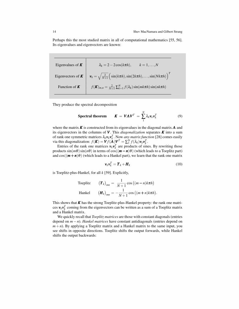
Perhaps this the most studied matrix in all of computational mathematics [55, 56].Its eigenvalues and eigenvectors are known:

Eigenvalues of KKK λk = 2−2cos(kπh), k = 1, . . . ,N

Eigenvectors of KKK vvvk =√

2N+1

(sin(kπh),sin(2kπh), . . . ,sin(Nkπh)

)T

Function of KKK f (KKK)m,n =2

N+1 ∑Nk=1 f (λk)sin(mkπh)sin(nkπh)

They produce the spectral decomposition

Spectral theorem KKK = VVVΛΛΛVVV T =N

∑1

λkvvvkvvvTk (9)

where the matrix KKK is constructed from its eigenvalues in the diagonal matrix ΛΛΛ andits eigenvectors in the columns of VVV . This diagonalization separates KKK into a sumof rank one symmetric matrices λkvvvkvvvT

k . Now any matrix function [28] comes easilyvia this diagonalization: f (KKK) =VVV f (ΛΛΛ)VVV T = ∑

N1 f (λk)vvvkvvvT

k .Entries of the rank one matrices vvvkvvvT

k are products of sines. By rewriting thoseproducts sin(mθ)sin(nθ) in terms of cos((mmm−−−nnn)θ) (which leads to a Toeplitz part)and cos((mmm+++nnn)θ) (which leads to a Hankel part), we learn that the rank one matrix

vvvkvvvTk = TTT k +HHHk (10)

is Toeplitz-plus-Hankel, for all k [59]. Explicitly,

Toeplitz(TTT k)

mn =1

N +1cos((m−−−n)kπh

)Hankel

(HHHk)

mn = − 1N +1

cos((m+++n)kπh

).

This shows that KKK has the strong Toeplitz-plus-Hankel property: the rank one matri-ces vvvkvvvT

k coming from the eigenvectors can be written as a sum of a Toeplitz matrixand a Hankel matrix.

We quickly recall that Toeplitz matrices are those with constant diagonals (entriesdepend on m−n). Hankel matrices have constant antidiagonals (entries depend onm+ n). By applying a Toeplitz matrix and a Hankel matrix to the same input, yousee shifts in opposite directions. Toeplitz shifts the output forwards, while Hankelshifts the output backwards:


Toeplitz

b ac b a

c b ac b

0 01 00 10 0

=

ab ac b

c

forward shift

Hankel

a b

a b ca b cb c

0 01 00 10 0

=

a

a bb cc

backward shift

Combining (10) with (9), we now see f (KKK) as the sum of a Toeplitz matrix anda Hankel matrix:

Matrix function f (KKK) = VVV f (ΛΛΛ)VVV T =N

∑1

f (λk)(TTT k +HHHk)

=N

∑1

f (λk)TTT k︸︷︷︸Toeplitz

+N

∑1

f (λk)HHHk︸︷︷︸Hankel

(11)

If we choose f (z) = z−1, then we split the inverse matrix into Toeplitz and Hankelparts: KKK−1 = TTT +HHH. With N = 3, this TTT and HHH are

KKK−1 =14

3 2 12 4 21 2 3

=18

5 2 −12 5 2−1 2 5

+18

1 2 32 3 23 2 1

.In summary, the matrix KKK, and all functions of that matrix, are Toeplitz-plus-

Hankel [59]. In the sequel, we make the particular choice f (z) = exp(±it√

z/∆x)or its real part, f (z) = cos(t

√z/∆x). Then f (KKK) solves a wave equation.

Before we proceed to the wave equation, we make one small observation aboutthe example of the convection-diffusion operator (PPP+DDD) in (4). It is an importantinstance of a nonsymmetric matrix where the pseudospectra plays a role in the anal-ysis [49]. That nonsymmetric matrix certainly does not have the strong Toeplitz-plus-Hankel property. However, with the help of a simple diagonal matrix ZZZ thesimilar matrix SSS≡ ZZZ(PPP+DDD)ZZZ−1 is symmetric, and SSS does have the strong Toeplitz-plus-Hankel property. The ith diagonal entry zi = ZZZi,i is found by setting z1 = 1, andzi+1 = zi

√bi/ai, where ai = MMMi+1,i, and bi = MMMi,i+1, and MMM = (PPP+DDD). We hope

to explore Toeplitz-plus-Hankel properties for convection-diffusion operators in thefuture.


4.2 The wave equation is Toeplitz-plus-Hankel

Our model problem is on an interval −1 ≤ x ≤ 1 with zero Dirichlet boundaryconditions u(−1, t) = u(1, t) = 0. The second derivative uxx is replaced by sec-ond differences at the mesh points x =−1, . . . ,−2∆x,−∆x,0,∆x,2∆x, . . . ,1, where∆x = 2/(N−1). The familiar wave equation can be approximated with the help ofthe second difference matrix KKK:

Wave equation∂ 2

∂ t2 uuu =∂ 2

∂x2 uuu becomesd2

dt2 uuu =− KKK∆x2 uuu. (12)

Time remains continuous in this finite difference, semi-discrete approximation. Onesolution to the semi-discrete approximation in (12) involves exponentials or cosinesof matrices:

Solution uuu(t) = f (KKK)uuu(0) = cos(

t√

KKK/∆x)

uuu(0).

Our purpose here is to apply the Toeplitz-plus-Hankel splitting, so we again setTTT = ∑k f (λk)TTT k and HHH = ∑k f (λk)HHHk, with TTT k and HHHk as in (10). Now with f (z) =cos(t

√z/∆x) in (11) we see this same solution as the sum of two parts:

uuu(t) = f (KKK)uuu(0) = TTT uuu(0)︸︷︷︸Toeplitz

+ HHHuuu(0).︸︷︷︸Hankel

Unlike the approximate splitting into products of exponentials discussed in the pre-vious sections of this chapter, here we see an exact splitting into a sum. Thus wehave split the wave equation into a Toeplitz part and a Hankel part. Now we canseparately investigate the behavior of the solutions coming from each part.

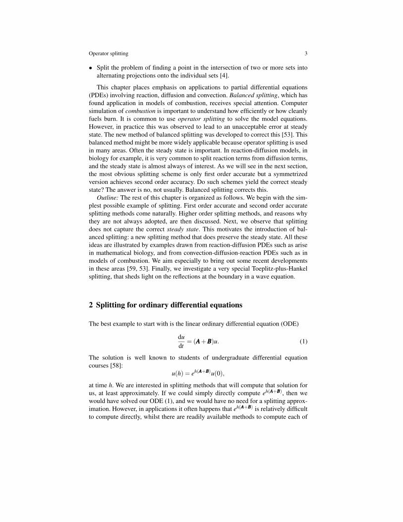
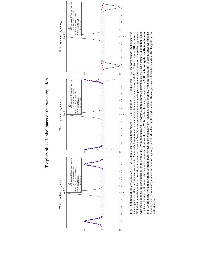
Figure 1 shows the exact solution to the wave equation via d’Alembert’s for-mula, as if the equation were on the whole real line with no boundaries. We usethis as a reference to compare to the solution of the same problem with Dirichletboundary conditions. We see the consequences of the boundary in the differencesbetween these solutions. Figure 1 also shows, separately, the solutions coming fromthe Toeplitz part (TTT uuu(0)) and the Hankel part (HHHuuu(0)). Their sum solves the Dirich-let problem exactly. The most interesting behavior happens at the boundary. Beforereaching the boundary, the solution is essentially Toeplitz. After reaching the bound-ary, the solution is essentially Hankel. The reflection at the boundary comes fromthe Hankel part of the operator.

The Toeplitz-plus-Hankel splitting described here is very special, but in this ex-ample the splitting does show reflections at the boundary in a new light: the reflec-tions come from the Hankel part of the operator. The design of absorbing boundaryconditions, or perfectly matched layers, is a big subject in computational science,that we will leave untouched [17, 27, 35]. We conjecture that Figure 1 can be under-stood by the method of images [59, 23]. That would involve identifying the solutionof the Dirichlet boundary condition version of the problem here with the solution ofa closely related problem having periodic boundary conditions. Periodic behavior is


far from ideal when designing absorbing boundary conditions – we don’t want thewave to come back to the domain later. Nevertheless, whilst the approximation ofthe Sommerfeld boundary condition results in a small reflection here, it is intriguingthat the Toeplitz part of the solution is seemingly reflectionless in Figure 1.

Outlook

This chapter introduced the basic ideas behind operator splitting methods. We fo-cused on the application of splitting methods to solve differential equations. Histor-ically, that has been their greatest application, though by now the splitting idea hasfound wide applications such as in optimization. We reviewed some of the main ap-plications in biology especially, such as splitting reaction terms from diffusion termsin reaction-diffusion PDEs. Operator splitting is an old idea of numerical analysis,so it is pleasing that new ideas and new applications keep appearing even today.Perhaps one of the biggest contemporary applications of splitting involves couplingmodels across scales, such as appropriate coupling of mesoscopic reaction diffusionmaster equation models to finer, microscopic models [19, 18, 26, 25]. On that front,no doubt more great work on splitting methods is still to come.

Toep

litz-

plus

-Han

kelp

arts

ofth

ew

ave

equa

tion

−1

−0.

8−

0.6

−0.

4−

0.2

00.

20.

40.

60.

81

−0.

50

0.51

x

Wav

e eq

uatio

n

utt =

c u

xx

t =

0.8

u(0)

u(t)

via

exa

ct D

Ale

mbe

rt fo

rmul

aU

(t)

via

K w

ith D

irich

let

U(t

) vi

a S

omm

erfe

ldT

oepl

itz p

art

Han

kel p

art

−1

−0.

8−

0.6

−0.

4−

0.2

00.

20.

40.

60.

81

−0.

50

0.51

x

Wav

e eq

uatio

n

utt =

c u

xx

t =

1

u(0)

u(t)

via

exa

ct D

Ale

mbe

rt fo

rmul

aU

(t)

via

K w

ith D

irich

let

U(t

) vi

a S

omm

erfe

ldT

oepl

itz p

art

Han

kel p

art

−1

−0.

8−

0.6

−0.

4−

0.2

00.

20.

40.

60.

81

−0.

50

0.51

x

Wav

e eq

uatio

n

utt =

c u

xx

t =

1.2

u(0)

u(t)

via

exa

ct D

Ale

mbe

rt fo

rmul

aU

(t)

via

K w

ith D

irich

let

U(t

) vi

a S

omm

erfe

ldT

oepl

itz p

art

Han

kel p

art

Fig.

1So

lutio

nsof

the

wav

eeq

uatio

nu t

t=

u xx

atth

ree

snap

shot

sin

time:

befo

re(t=

0.8)

,dur

ing

(t=

1.0)

and

afte

r(t=

1.2)

the

wav

ere

ache

sth

ebo

unda

ryof

the

com

puta

tiona

ldom

ain.

The

exac

tsol

utio

n(d

’Ale

mbe

rt’s

form

ula)

and

vari

ous

finite

diff

eren

ceap

prox

imat

ions

,with

∆x=

2/(N−

1),N

=20

1,ar

esh

own.

With

the

Som

mer

feld

radi

atio

nco

nditi

on,u

x=±

u t,a

tthe

ends

ofou

rfini

teco

mpu

tatio

nald

omai

n,w

eho

peou

rcom

puta

tiona

lsol

utio

nis

inpe

rfec

tagr

eem

ent

with

the

solu

tion

toth

ew

ave

equa

tion

onth

ew

hole

line

(with

nobo

unda

ry).

How

ever

,afin

itedi

ffer

ence

appr

oxim

atio

nof

the

Som

mer

feld

cond

ition

isno

tex

act,

and

the

smal

lrefl

ectio

nvi

sibl

eat

t=1.

2is

am

anif

esta

tion

ofth

eer

ror.

With

Dir

ichl

etbo

unda

ryco

nditi

ons,

inKK K

,the

solu

tion

split

sexa

ctly

into

the

sum

ofa

Toep

litz

solu

tion

and

aH

anke

lsol

utio

n.B

efor

ere

achi

ngth

ebo

unda

ry,t

heso

lutio

nis

pure

lyTo

eplit

z,w

hile

the

Han

kelp

arti

sab

sent

.Aft

erre

achi

ngth

ebo

unda

ry,i

tis

the

othe

rway

arou

nd:t

heso

lutio

nis

pure

lyH

anke

l,w

hile

the

Toep

litz

part

isab

sent

.Han

kelp

arts

com

efr

omth

ebo

unda

ry.T

heTo

eplit

zpa

rtis

refle

ctio

nles

s.


References

1. Ascher, U., Ruuth, S., Wetton, B.: Implicit-explicit methods for time-dependent partial differ-ential equations. SIAM Journal on Numerical Analysis (1995)

2. Asmussen, S., Glynn, P.W.: Stochastic Simulation: Algorithms and Analysis. Springer (2007)3. Blanes, S., Casas, F., Chartier, P., Murua, A.: Optimized high-order splitting methods for some

classes of parabolic equations. Math. Comput. (2012)4. Boyd, S., Parikh, N., Chu, E., Peleato, B., Eckstein, J.: Distributed Optimization and Statistical

Learning via the Alternating Direction Method of Multipliers. Foundations and Trends inMachine Learning pp. 1–122 (2011)

5. Butcher, J.: Numerical Methods for Ordinary Differential Equations. Wiley (2003)6. Cao, Y., Gillespie, D.T., Petzold, L.R.: The slow-scale stochastic simulation algorithm. J.

Chem. Phys. 122, 014,116–1–18 (2005)7. Chorin, A.J.: Numerical solution of the Navier-Stokes equations. Math. Comp. pp. 745–762

(1968)8. Dahlquist, G.: Convergence and stability in the numerical integration of ordinary differential

equations. Math. Scand. pp. 33–53 (1956)9. Dahlquist, G.: A special stability problem for linear multistep methods. BIT Numerical Math-

ematics pp. 27–43 (1963)10. Dahlquist, G., Bjork, A.: Numerical Methods. Prentice-Hall (1974)11. Daubechies, I.: Ten Lectures on Wavelets. SIAM (1992)12. Descombes, S.: Convergence of a splitting method of high order for reaction-diffusion sys-

tems. Mathematics of Computation 70(236), 1481–1501 (2001)13. Descombes, S., Schatzman, M.: Directions alternees d’ordre eleve en reaction-diffusion.

Comptes Rendus de l’Academie des Sciences. Serie 1, Mathematique 321(11), 1521–1524(1995)

14. Douglas, J., Rachford, H.H.: On the numerical solution of heat conduction problems in twoand three space variables. Trans. Amer. Math. Soc. pp. 421–439 (1956)

15. E, W., Liu, D., Vanden-Eijnden, E.: Nested stochastic simulation algorithm for chemical ki-netic systems with disparate rates. J. Chem. Phys. 123(19), 194,107 (2005)

16. Engblom, S.: Strong convergence for split-step methods in stochastic jump kinetics (2014).http://arxiv.org/abs/1412.6292

17. Engquist, B., Majda, A.: Absorbing boundary conditions for numerical simulation of waves.Proc Natl Acad Sci U S A 74, 765–1766 (1977)

18. Ferm, L., Lotstedt, P.: Numerical method for coupling the macro and meso scales in stochasticchemical kinetics. BIT Numerical Mathematics 47(4), 735–762 (2007)

19. Ferm, L., Lotstedt, P., Hellander, A.: A hierarchy of approximations of the master equationscaled by a size parameter. J. Sci. Comput. 34, 127–151 (2008)

20. Giles, M.: Multi-level Monte Carlo path simulation. Operations Research 56, 607–617 (2008)21. Goldstein, T., Osher, S.: The Split Bregman Method for L1-Regularized Problems. SIAM

Journal on Imaging Sciences 2(2), 323–343 (2009)22. Golub, G.H., Van Loan, C.F.: Matrix Computations. Johns Hopkins (1996)23. Haberman, R.: Applied Partial Differential Equations. Prentice Hall (2013)24. Hairer, E., Lubich, C., Wanner, G.: Geometric numerical integration: Structure-preserving al-

gorithms for ordinary differential equations. Springer (2006)25. Hellander, A., Hellander, S., Lotstedt, P.: Coupled mesoscopic and microscopic simulation of

stochastic reaction-diffusion processes in mixed dimensions. Multiscale Model. Simul. pp.585–611 (2012)

26. Hellander, A., Lawson, M., Drawert, B., Petzold, L.: Local error estimates for adaptive simu-lation of the reaction-diffusion Master Equation via operator splitting. J. Comput. Phys (2014)

27. Higdon, R.: Numerical Absorbing Boundary Conditions for the Wave Equation. Mathematicsof Computation 49, 65–90 (1987)

28. Higham, N.J.: Functions of Matrices. SIAM (2008)29. Horn, R., Johnson, C.: Matrix Analysis. Cambridge University Press (2013)


30. Hundsdorfer, W., Verwer, J.: Numerical Solution of Time-Dependent Advection-Diffusion-Reaction Equations. Springer (2003)

31. Iserles, A.: A First Course in the Numerical Analysis of Differential Equations. CambridgeUniversity Press (1996)

32. Jahnke, T., Altintan, D.: Efficient simulation of discrete stochastic reaction systems with asplitting method. BIT 50, 797–822 (2010)

33. Lax, P.D., Richtmyer, R.D.: Survey of the stability of linear finite difference equations. Comm.Pure Appl. Math pp. 267–293 (1956)

34. Lee, J., Fornberg, B.: A split step approach for the 3-D Maxwell’s equations. J. Comput. Appl.Math. 158, 485–505 (2003)

35. Loh, P.R., Oskooi, A.F., Ibanescu, M., Skorobogatiy, M., Johnson, S.G.: Fundamentalrelation between phase and group velocity, and application to the failure of perfectlymatched layers in backward-wave structures. Phys. Rev. E 79, 065,601 (2009). DOI10.1103/PhysRevE.79.065601. URL http://link.aps.org/doi/10.1103/PhysRevE.79.065601

36. Lubich, C., Oseledets, I.: A projector-splitting integrator for dynamical low-rank approxima-tion. BIT Numerical Mathematics 54, 171–188 (2014)

37. MacNamara, S., Burrage, K., Sidje, R.: Application of the Strang Splitting to the chemicalmaster equation for simulating biochemical kinetics. The International Journal of Computa-tional Science 2, 402–421 (2008)

38. MacNamara, S., Burrage, K., Sidje, R.: Multiscale Modeling of Chemical Kinetics via theMaster Equation. SIAM Multiscale Model. & Sim. 6(4), 1146–1168 (2008)

39. Maini, P.K., Baker, R.E., Chuong, C.M.: The Turing model comes of molecular age. Science314, 1397–1398 (2006)

40. Marchuk, G.I.: Some application of splitting-up methods to the solution of mathematicalphysics problems. Aplikace matematiky pp. 103–132 (1968)

41. Marchuk, G.I.: Splitting and alternating direction methods. In: P. Ciarlet, J. Lions (eds.) Hand-book of Numerical Analysis, vol. 1, pp. 197–462. North-Holland, Amsterdam (1990)

42. McLachlan, R., Quispel, G.: Splitting methods. Acta Numer. 11, 341–434 (2002)43. Moler, C., Van Loan, C.: Nineteen Dubious Ways to Compute the Exponential of a Matrix, 25

Years Later. SIAM Review 45(1), 3–49 (2003)44. Murray, J.: Mathematical Biology: An Introduction. New York : Springer (2002)45. Ninomiya, S., Victoir, N.: Weak approximation of stochastic differential equations and appli-

cation to derivative pricing. Applied Mathematical Finance 15 (2008)46. Pavliotis, G., Stuart, A.: Multiscale Methods: Averaging and Homogenization. Springer

(2008)47. Peaceman, D.W., Rachford Jr., H.H.: The numerical solution of parabolic and elliptic differ-

ential equations. Journal of the Society for Industrial and Applied Mathematics (1955)48. Rauch, J.: The Turing Instability. URL: http://www.math.lsa.umich.edu/ rauch/49. Reddy, S.C., Trefethen, L.N.: Pseudospectra of the convection-diffusion operator. SIAM J.

Appl. Math (1994)50. Ropp, D., Shadid, J.: Stability of operator splitting methods for systems with indefinite oper-

ators: Reaction-diffusion systems. Journal of Computational Physics 203, 449–466 (2005)51. Saad, Y.: Iterative Methods for Sparse Linear Systems. SIAM, Society for Industrial and

Applied Mathematics, Philadelphia (2003)52. Schatzman, M.: Toward non commutative numerical analysis: High order integration in time.

Journal of Scientific Computing 17, 99–116 (2002)53. Speth, R., Green, W., MacNamara, S., Strang, G.: Balanced splitting and rebalanced splitting.

SIAM Journal of Numerical Analysis 51(6), 3084–3105 (2013)54. Strang, G.: On the construction and comparison of difference schemes. SIAM J. Numer. Anal.

5(2), 506–517 (1968)55. Strang, G.: Computational Science and Engineering. Wellesley-Cambridge Press (2007)56. Strang, G.: Introduction to Linear Algebra. Wellesley-Cambridge Press (2009)57. Strang, G.: Essays in Linear Algebra. Wellesley-Cambridge Press (2012)58. Strang, G.: Differential Equations and Linear Algebra. Wellesley-Cambridge Press (2014)


59. Strang, G., MacNamara, S.: Functions of difference matrices are Toeplitz plus Hankel. SIAMReview 56(3), 525–546 (2014)

60. Trefethen, L.: Numerical analysis. In: T. Gowers, J. Barrow-Green, I. Leader (eds.) PrincetonCompanion to Mathematics, pp. 604–615. Princeton University Press (2008)

61. Trefethen, L., Embree, M.: Spectra and Pseudospectra: The Behavior of Nonnormal Matricesand Operators. Princeton University Press (2005)

62. Usadi, A., Dawson, C.: 50 years of ADI methods: Celebrating the contributions of Jim Dou-glas, Don Peaceman, and Henry Rachford. SIAM News 39 (2006)

63. Wanner, G.: Dahlquist’s classical papers on stability theory. BIT Numerical Mathematics 46,671–683 (2006)

64. Widom, H.: Toeplitz matrices. In: I.I. Hirschman (ed.) Studies in Real and Complex Analysis.Prentice-Hall (1965)

65. Yoshida, H.: Construction of higher order symplectic integrators. Phys. Lett. A. 150, 262–268(1990)

Documents

Operator splitting - UCLAwotaoyin/splittingbook/ch3-macnamara-strang.pdf · Operator splitting Shev MacNamara and Gilbert Strang Abstract Operator splitting is a numerical method