Embed Size (px)
Citation preview

Operational Transfer Path Analysis A Study of Source Contribution Predictions at Low Frequency Master’s Thesis in the Master’s programme in Sound and Vibration
MIHKEL TOOME Department of Civil and Environmental Engineering Division of Applied Acoustics Vibroacoustics Group CHALMERS UNIVERSITY OF TECHNOLOGY Göteborg, Sweden 2012 Master’s Thesis 2012:141

MASTER’S THESIS 2012:141
Operational Transfer Path Analysis:
A Study of Source Contribution Predictionsat Low Frequency
Mihkel Toome
Department of Civil and Environmental EngineeringDivision of Applied Acoustics
Vibroacoustics GroupCHALMERS UNIVERSITY OF TECHNOLOGY
Göteborg, Sweden 2012

Operational Transfer Path Analysis:A Study of Source Contribution Predictions at Low Frequency
© Mihkel Toome, 2012
Master’s Thesis 2012:141
Department of Civil and Environmental EngineeringDivision of Applied AcousticsVibroacoustics GroupChalmers University of TechnologySE-41296 GöteborgSweden
Tel. +46 (0)31 772 1000
Reproservice / Department of Civil and Environmental EngineeringGöteborg, Sweden 2012

Operational Transfer Path Analysis:A Study of Source Contribution Predictions at Low FrequencyMaster’s Thesis in the Master’s Programme Sound and VibrationMIHKEL TOOMEDepartment of Civil and Environmental EngineeringDivision of Applied AcousticsVibroacoustics GroupChalmers University of Technology
Abstract
The operational transfer path analysis (OTPA) method is a variation of the classicaltransfer path analysis (TPA) method, both of which are used particularly for noise,vibration and harshness (NVH) testing in the vehicle industry. The methods differsuch that classical TPA requires a physical isolation of the critical source-receiver pathsto eliminate cross-talk prior to determining the frequency response functions (FRFs),whereas OTPA uses singular value decomposition (SVD) and principal componentanalysis (PCA) for cross-talk cancellation (CTC), prior to computing the transmissi-bility of each critical path.
In some cases, it has been found that the OTPA results yield an over-prediction of theairborne sound contribution in the low frequency range (20 to 100 Hz). This over-prediction seems to occur when several microphones are placed within close proximityof each other (i.e. within a fraction of the wavelength).
This thesis begins with a study of the underlying theory for the classical TPA and theOTPA methods. The limitations and potential sources of error for each method arediscussed. The OTPA method is further studied by way of an implementation usingMATLAB. The OTPA script is tested and validated using a virtual test setup (VTS),consisting of two sources and one receiver.
Next, the VTS is used to study several simplified OTPA scenarios. Subsequently, theover-prediction of the airborne sound contribution is recreated using the VTS andOTPA scripts. The reasons for the over-prediction of the airborne sound contributionare identified and discussed.
Keywords: Operational Transfer Path Analysis, OTPA, Cross-Talk Cancellation, CTC,Low Frequency, Source Contribution,
iii


Acknowledgements
This master’s thesis topic was proposed by Müller-BBM Scandinavia AB, and the workhas been carried out with guidance from engineers from both Müller-BBM ScandinaviaAB and Müller-BBM VibroAkustik Systeme GmbH.
First and foremost, I would like to thank my advisor at Müller-BBM Scandinavia, Dr.Juha Plunt, who’s technical expertise, experience and guidance have been invaluablein completing this thesis work. Also, thank-you to Martin Lohrmann at Müller-BBMVibroAkustik Systeme for taking the time to meet with me to discuss OTPA and for hissuggestions on what aspects of the method would be interesting to study.
This thesis project is the culmination of two years of study at the Division of AppliedAcoustics at Chalmers University of Technology. Thank-you to all my colleagues andto all the staff for the informative lectures, labs, exercises, projects and discussions. Inparticular, thank-you to my thesis supervisor, Professor Wolfgang Kropp, who’s in-sight, guidance and encouragement have helped make this thesis project a rewardingexperience.
Most importantly, thank-you to my wife, Heili, for her constant love and support, es-pecially during these past two years.
Mihkel ToomeGöteborg, June 2012
v


Contents
Abstract iii
Acknowledgements v
Contents vi
List of Figures ix
List of Abbreviations xi
1. Introduction 11.1. Case Study: Airborne Sound Over-Prediction Using OTPA . . . . . . . . 1
1.1.1. OTPA Measurement Setup . . . . . . . . . . . . . . . . . . . . . . 21.1.2. OTPA Contribution Analysis Results . . . . . . . . . . . . . . . . 31.1.3. Case Study Conclusions . . . . . . . . . . . . . . . . . . . . . . . . 4
1.2. Thesis Structure . . . . . . . . . . . . . . . . . . . . . . . . . . . . . . . . . 51.2.1. Hypotheses . . . . . . . . . . . . . . . . . . . . . . . . . . . . . . . 51.2.2. Overview . . . . . . . . . . . . . . . . . . . . . . . . . . . . . . . . 6
2. Basic Principles of (Operational) Transfer Path Analysis 72.1. The Classical Transfer Path Analysis (TPA) Method . . . . . . . . . . . . 7
2.1.1. The Frequency Response Function (FRF) . . . . . . . . . . . . . . 72.1.2. Determining the Operational Excitation Force Function . . . . . . 92.1.3. Limitations of The Classical TPA Method . . . . . . . . . . . . . . 10
2.2. The Operational Transfer Path Analysis (OTPA) Method . . . . . . . . . 112.2.1. The Operational Transfer Function . . . . . . . . . . . . . . . . . . 112.2.2. The Cross-Talk Cancellation Method . . . . . . . . . . . . . . . . . 142.2.3. Response Synthesis . . . . . . . . . . . . . . . . . . . . . . . . . . . 172.2.4. OTPA Limitations and Potential Sources of Error . . . . . . . . . . 19
3. Implementation of OTPA and CTC 213.1. MATLAB Script: Description of Key Functions . . . . . . . . . . . . . . . 23
3.1.1. Singular Value Decomposition . . . . . . . . . . . . . . . . . . . . 233.1.2. Principal Component Analysis and Cross-Talk Cancellation . . . 233.1.3. Response Synthesis and Contribution Analysis . . . . . . . . . . . 24
vii
Contents
4. The Virtual Test Setup 254.1. Virtual Test Setup Layout . . . . . . . . . . . . . . . . . . . . . . . . . . . 254.2. Source Signals - Background Theory . . . . . . . . . . . . . . . . . . . . . 254.3. VTS and OTPA Parameters . . . . . . . . . . . . . . . . . . . . . . . . . . 27
4.3.1. VTS Paramaters . . . . . . . . . . . . . . . . . . . . . . . . . . . . . 274.3.2. OTPA Parameters . . . . . . . . . . . . . . . . . . . . . . . . . . . . 28
5. Analysis 295.1. Analysis Outline . . . . . . . . . . . . . . . . . . . . . . . . . . . . . . . . 295.2. OTPA Validation: CTC and Noise Removal Using PCA . . . . . . . . . . 315.3. OTPA of Two Airborne Noise Sources . . . . . . . . . . . . . . . . . . . . 33
5.3.1. Varying Distance Between Two Correlated Sources . . . . . . . . 345.3.2. Varying Distance Between Two Uncorrelated Sources . . . . . . . 385.3.3. Discussion and Summary of Results . . . . . . . . . . . . . . . . . 42
5.4. OTPA of Correlated Structure-Borne and Airborne Noise Sources . . . . 435.4.1. Effects of Varying Distance of Additional Airborne Source MPs . 435.4.2. Varying The Number of Reference MPs . . . . . . . . . . . . . . . 465.4.3. Discussion and Summary of Results . . . . . . . . . . . . . . . . . 49
6. Summary and Conclusions 516.1. Suggestions for Future Work . . . . . . . . . . . . . . . . . . . . . . . . . . 52
References 53
A. MATLAB Script 55A.1. MATLAB Script - Two Airborne Noise Sources . . . . . . . . . . . . . . . 55
A.1.1. OTPA Script (otpa.m) . . . . . . . . . . . . . . . . . . . . . . . . . 55A.1.2. Function to Define The Virtual Test Setup Layout (dist.m) . . . . 58A.1.3. Function to Define The Source Signal (source.m) . . . . . . . . . . 59
A.2. MATLAB Script - Airborne and Structure-Borne Sources . . . . . . . . . 61A.2.1. OTPA Script (otpa_sbs.m) . . . . . . . . . . . . . . . . . . . . . . . 61A.2.2. Function to Define The Virtual Test Setup Layout (dist_sbs.m) . . 65A.2.3. Function to Define The Source Signal (source_sbs.m) . . . . . . . 66
A.3. Function to Plot Sound Field (contourmesh.m) . . . . . . . . . . . . . . . 68A.4. MATLAB Script - Airborne and Structure-Borne Sources, Varied Number
of Reference MPs . . . . . . . . . . . . . . . . . . . . . . . . . . . . . . . . 69A.4.1. OTPA Script (otpa_sbs_num.m) . . . . . . . . . . . . . . . . . . . 69A.4.2. Function to Define The Virtual Test Setup Layout (dist_sbs_num.m) 72A.4.3. Function to Define The Source Signal (source_sbs_num.m) . . . . 73A.4.4. Function to Plot Sound Field (contourmesh_num.m) . . . . . . . 74
viii CHALMERS, Master’s Thesis 2012:141

List of Figures
1.1. OTPA microphone positions . . . . . . . . . . . . . . . . . . . . . . . . . . 21.2. Response contribution analysis (12 microphone positions) . . . . . . . . 31.3. Response contribution analysis (6 microphone positions) . . . . . . . . . 4
3.1. OTPA Program Flow Chart . . . . . . . . . . . . . . . . . . . . . . . . . . 22
4.1. Virtual Test Setup Schematic . . . . . . . . . . . . . . . . . . . . . . . . . . 26
5.1. VTS layout (4 reference MPs) . . . . . . . . . . . . . . . . . . . . . . . . . 315.2. Response synthesis and principal component contribution . . . . . . . . 325.3. Sound field – correlated sources (QA = QB, fA = fB) . . . . . . . . . . . . 345.4. Source contribution – correlated sources (QA = QB, fA = fB) . . . . . . . 355.5. Sound field – correlated sources (QA = 2QB, fA = fB) . . . . . . . . . . . 365.6. Source contribution – correlated sources (QA = 2QB, fA = fB) . . . . . . 375.7. Sound field at fA – uncorrelated sources ( fA 6= fB) . . . . . . . . . . . . . 385.8. Sound field at fB – uncorrelated sources ( fA 6= fB) . . . . . . . . . . . . . 395.9. Source contribution at fA – uncorrelated sources ( fA 6= fB) . . . . . . . . 405.10. Source contribution at fB – unorrelated sources ( fA 6= fB) . . . . . . . . . 415.11. VTS layout – varying additional ABS MP distance . . . . . . . . . . . . . 445.12. Source contribution – varying additional ABS MP distance . . . . . . . . 455.13. VTS layout – varying number of ABS reference MPs . . . . . . . . . . . . 465.14. Source contribution – varying number of ABS reference MPs (LSBS = LABS) 475.15. Source contribution – varying number of ABS reference MPs (LSBS =
2LABS) . . . . . . . . . . . . . . . . . . . . . . . . . . . . . . . . . . . . . . 48
ix


List of Abbreviations
ABS Airborne SoundCTC Cross-Talk CancellationDFT Discrete Fourier TransformDOF(s) Degree(s) of FreedomFRF Frequency Response FunctionMBBMS Müller-BBM ScandinaviaMBBM-VAS Müller-BBM VibroAkustik SystemeMIMO Multiple Input/Multiple OutputMP(s) Measurement Point(s)NTF Noise Transfer FunctionOTPA Operational Transfer Path AnalysisPCA Principal Component AnalysisPC(s) Principal Component(s)SBS Structure-Borne SoundSVD Singular Value DecompositionTPA Transfer Path AnalysisVTF Vibration Transfer FunctionVTS Virtual Test Setup
xi


1. Introduction
Operational transfer path (OTPA) analysis was introduced circa the mid-2000’s as analternative to the classical transfer path analysis (TPA) method, which has been usedfor NVH analysis in the automotive industry since the 1970’s. The main advantage ofthe OTPA method over the classical TPA method is that measurement of the frequencyresponse functions (FRFs) of the physically isolated critical paths is not necessary –therefore, a considerable amount of measurement and analysis time is saved by usingthe OTPA method.
The fundamental difference between the TPA and OTPA is that the TPA method deter-mines a force-response transfer path relationship (an FRF), whereas the OTPA methoddetermines a response-response transfer path relationship (a transmissibility). Bothmethods have their advantages and disadvantages – these, along with the underlyingtheory behind both analysis methods, are discussed in Chapter 2.
The focus of this master’s thesis is on a phenomenon that has recently transpired inthe OTPA measurement results for several analysis cases1: The OTPA method seemsto over-predict the airborne sound contribution when several microphones are used inclose proximity2. Furthermore, this over-prediction of airborne sound seems to lead toan under-prediction of structure-borne sound in the same frequency range – the energyin that frequency range seems to be erroneously shifted from the structure-borne soundcontribution to the airborne sound contribution.
The objective of this thesis work is to study the OTPA method and to determine whatis causing the erroneous source contribution prediction in the low frequency range.
1.1. Case Study: Airborne Sound Over-Prediction Using OTPA
In the following, a Müller-BBM Scandinavia AB (MBBMS) project for which the OTPAresults include the over-prediction of airborne sound (and under-prediction of structure-borne sound) is described.
1The phenomenon has been noticed for both stationary and vehicle pass-by OTPA results on Müller-BBMScandinavia AB projects.
2In this report, references to distances, such as "close proximity", are always relative to the wavelengthof the low frequency airborne sound.
1

1.1. Case Study: Airborne Sound Over-Prediction Using OTPA
This particular project involved the OTPA of a trailer-less road tractor1 during an idlingoperating condition.
1.1.1. OTPA Measurement Setup
Accelerometers and microphones were placed such that all of the critical sources andpaths were included in the analysis. The microphone positions are indicated in Fig-ure 1.1, which is a schematic of the tractor as seen from above. The microphones weremounted to be approximately 30-40 cm from the surface of the source, and measure-ments were taken outdoors (i.e. the free field can be assumed).
12 Microphones total
6 Microphones relatively close together (expcept intake)
6 Additional microphones
Cab
Intake at top of cab
Figure 1.1.: OTPA microphone positions
To compute the transfer functions, measurements of several operating conditions wereincluded in the analysis to ensure excitation of all relevant modes. The operating con-ditions used for the transfer function computation were: neutral run-up, neutral run-down and idle. The tractor was stationary for all measurements (i.e. no wind noise ortire rolling noise).
The measurement data was collected and analyzed using the MBBM-VAS measure-ment interface PAK® [15].
1a.k.a. lorry, transport truck, rig.
2 CHALMERS, Master’s Thesis 2012:141

1. Introduction
1.1.2. OTPA Contribution Analysis Results
The response contribution analysis results of an engine idle condition produced somestrange results. Referring to Figure 1.2b, note that the airborne sound (ABS) contribu-tion at 25 Hz is much more prominent, approximately 20 dB higher, than the structure-borne sound (SBS) contribution.
a. Campbell Plot (Idle) b. Contribution Analysis (25 Hz)
10 dB
SB
S T
OT
AL
AB
S T
OT
AL
TO
TA
L
Tim
e (s
)
Frequency (Hz) SPL (dB)
Figure 1.2.: Response contribution analysis (12 microphone positions)
A comparison of the actual measured response at the receiver position to the total re-sponse synthesis indicated that the results are accurate. However, previous experienceby MBBMS engineers suggested that the response contribution results are erroneous –at low frequencies, such as 25 Hz, a significant structure-borne sound contribution isexpected.
Since the analysis was conducted on an engine idle operating condition, it was decidedthat the tire, rear axle and engine cooling fan microphones are not measuring signifi-cant noise sources, and should therefore be excluded from the analysis. The OTPA wasconducted again, but this time with the measurement data from the six additional mi-crophone positions excluded from the analysis (refer to Figure 1.1 for the microphoneposition layout).
The OTPA response contribution results with the six additional microphones (tires, rearaxle and engine cooling fan) excluded are quite different than the results with all twelve
CHALMERS, Master’s Thesis 2012:141 3

1.1. Case Study: Airborne Sound Over-Prediction Using OTPA
microphones included in the analysis. Referring to Figure 1.3b, note that the airborneand structure-borne contributions are approximately equal at 25 Hz. The total responseat the receiver remains unchanged from the previous analysis case.
a. Campbell Plot (Idle) b. Contribution Analysis (25 Hz)
AB
S T
OT
AL
SB
S T
OT
AL
TO
TA
L
10 dB
Frequency (Hz)
Tim
e (s
)
SPL (dB)
Figure 1.3.: Response contribution analysis (6 microphone positions)
By excluding the six additional microphone positions from the OTPA, the predictedtotal airborne sound contribution dropped by approximately 5 dB, while the predictedtotal structure-borne sound contribution increased by approximately 15 dB. Further,most of the individual structure-borne source contributions also increased significantlyfor the latter case.
1.1.3. Case Study Conclusions
The results of these two cases lead to very different conclusions – For the first case(12 microphones positions), the contribution analysis results indicate that the airbornesound of the transmission is the critical source. For the second case (6 microphonepositions), the contribution analysis indicates that both the structure-borne (the cabmounts) and airborne (transmission) sources are significant.
Past experience by MBBMS engineers lead to a partiality towards the analysis resultswhich excluded the six additional microphone positions. Consequently, modifications
4 CHALMERS, Master’s Thesis 2012:141

1. Introduction
were made to the tractor in order to reduce the structure-borne sound contribution.The modifications were successful in reducing the overall sound pressure level at thereceiver, thus confirming that the contribution analysis results with the six additionalmicrophone positions excluded are more accurate than the results using all twelve mi-crophone positions.
Comparing the results of the two OTPA cases, refer to Figures 1.2 and 1.3, observe thatalthough the total airborne and structure-borne contributions change, the total soundpressure level remains the same. This indicates that by excluding the six additionalmicrophones, the acoustic energy is shifted from the airborne sound to the structure-borne sound in the contribution calculation.
1.2. Thesis Structure
This thesis is based on an investigation of why the erroneous source contribution de-scribed in the tractor OTPA case study has occured. In the following, the hypothesesare presented, and the thesis structure is outlined.
1.2.1. Hypotheses
The main hypotheses drawn from the results of the tractor OTPA case study are basedon the observation that the six additional microphones are not measuring a significantsource, therefore, it is possible that cross-talk from the other nearby significant contrib-utors creates a bias towards the airborne contribution in the results.
The bias towards airborne sound contribution occurs at low frequencies – in this casestudy at 25 Hz, however it can be generalized to the range of 20 to 100 Hz. This couldbe for one or more of the following reasons:
• The structure-borne sound contribution typically occurs in this low frequencyrange – It is possible that the energy is shifted from structure-borne to airbornesound, since both could include acoustic energy and may also be highly corre-lated in this frequency range.
• All of the microphone positions are within a fraction of the wavelength of thesource (e.g. for dry air at 20 �C the wavelength of a 25 Hz tone is 13.7 m). It ispossible that cross-talk cancellation between the reference microphone positionsis not effective since the sound pressure and phase is more or less the same at allmicrophone positions in the low frequency range.
CHALMERS, Master’s Thesis 2012:141 5

1.2. Thesis Structure
• The reference microphones are positioned close to the sources – It is possible thatthe results are influenced because the measurements are taken in the near field ofthe low frequency range.
1.2.2. Overview
The outline of this thesis is described as follows:
Chapter 2 begins with an explanation of the theory behind both the classical TPAmethod and OTPA method, including advantages and disadvantages for both. Alsoincluded in this chapter is an explanation of the cross-talk cancellation method as wellas reconstructing the signal as the response synthesis and for contribution analysis.
In Chapter 3, an implementation of the OTPA theory is discussed. The implementationis conducted using MATLAB®, with the relevant script included in Appendix A.
To validate the OTPA implementation, and to investigate the hypotheses proposed inSection 1.2.1, a virtual test setup (VTS) consisting of two sources and one receiver isdeveloped using MATLAB. Various VTS configurations are setup in order to study theOTPA method, and to attempt to recreate the airborne sound over-prediction. The VTSimplementation and various analyses are discussed in Chapters 4 and 5. An exampleof the relevant MATLAB script is included in Appendix A.
The conclusions drawn from the OTPA study are summarized in Chapter 6. The con-clusions include suggestions for practical rules of thumb for setting up an OTPA mea-surement.
6 CHALMERS, Master’s Thesis 2012:141

2. Basic Principles of (Operational) TransferPath Analysis
2.1. The Classical Transfer Path Analysis (TPA) Method
The transfer path analysis (TPA) method is used particularly in the automotive indus-try to for the analysis of the different contributions of noise and/or vibration at a partic-ular receiver position (e.g. the driver and passenger positions in a vehicle). The methodaims to identify propagation paths from the various airborne and structure-borne noisesources (e.g. engine, gearbox, intake, exhaust, tire noise) by using a load-response lin-ear relationship model.
2.1.1. The Frequency Response Function (FRF)
The classical TPA method identifies the frequency response functions (FRF) of the var-ious source-receiver paths by using a known artificial excitation, for example, using ashaker as a vibration source or using a loudspeaker as an airborne source, and mea-suring the response at the receiver. The resulting FRFs are uniquely determined by theproperties of the linear multiple input/multiple output (MIMO) system that relates theresponse to the input excitation force (structure-borne) and/or volume velocity (air-borne) [1]. Note that the classical TPA method can also be applied reciprocally to de-termine the FRFs - Meaning that the excitation is applied at the receiver position andthe response is measured at the source position [20].
In some cases, the use of a shaker/loudspeaker is not possible, and the operationalforce is used to determine the FRF. However, in this case, to accurately determine thetransfer function, the input force must also be accurately determined by measurementand/or calculation [8, 11].
Once the FRF has been determined, the predicted response at the receiver is calcu-lated by multiplying the operational force with the measured FRF. Assuming a linearrelationship between excitation point and response point, the response at the receiver(sound pressure level or vibration) is determined by:
7

2.1. The Classical Transfer Path Analysis (TPA) Method
y(jw) = H(jw)x(jw) (2.1)
Where the response (or output), y(jw), is related to the input, x(jw), by the transferfunction (FRF), H(jw). The dependancy on phase and frequency is indicated by (jw).Note that in the classical TPA, the transfer function is the FRF between input and out-put, although sometimes this may also be referred to as the noise transfer function(NTF) and/or the vibration transfer function (VTF).
In order to calculate the total response at the receiver, all source-path-receiver configu-rations must be included in the analysis. This requires that all potential noise sourcesand related paths must be measured (e.g. engine, transmission, exhaust and intake,tires, etc). The total response1 (i.e. sound pressure and/or vibration) at the receiveris a superposition of all the individual contributions and is obtained by summing thecontribution of the product of all input excitations and transfer paths, as is describedby Equation 2.2.
ym(jw) =N
Ân=1
Hmn(jw)xn(jw) (2.2)
Where:ym(jw) is the response at the receiver located at point m;Hmn(jw) is the FRF between point m and the input excitation applied to path n;xn(jw) is the input excitation force function applied to path n
In general, the input is a force (Fn) or volume velocity (Qj), and the response is a soundpressure (pm) or vibration (xm, for acceleration). If both structural and acoustic inputloads are considered, the response at the receiver is expressed as:
pm(w) =k
Ân=1
Hn(w)Fn(w) +r
Âj=1
Hj(w)Qj(w) (2.3)
Where:pm(w) is the response (sound pressure) at the receiver point m;Fn is the force input, or structural load, at point n (source of structure borne noise);Qj is the volume velocity input , or acoustic load, at point j (source of airborne noise);Hn and Hj are the corresponding FRFs.
Note that in Equation 2.3 the airborne and structure borne contributions are treatedsimilarly. For the classical TPA method, the measured response is typically sound or
1Note that the contribution of wind noise is usually not included in the TPA model since the excitationforce/noise is distributed over an area (over the entire exterior area of the vehicle).
8 CHALMERS, Master’s Thesis 2012:141
2. Basic Principles of (Operational) Transfer Path Analysis
vibration, and the input is a force. For the sake of simplicity, the following discussionon the TPA theory will focus on the structure-borne case.
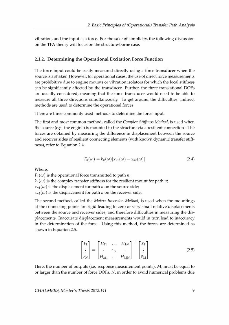
2.1.2. Determining the Operational Excitation Force Function
The force input could be easily measured directly using a force transducer when thesource is a shaker. However, for operational cases, the use of direct force measurementsare prohibitive due to engine mounts or vibration isolators for which the local stiffnesscan be significantly affected by the transducer. Further, the three translational DOFsare usually considered, meaning that the force transducer would need to be able tomeasure all three directions simultaneously. To get around the difficulties, indirectmethods are used to determine the operational forces.
There are three commonly used methods to determine the force input:
The first and most common method, called the Complex Stiffness Method, is used whenthe source (e.g. the engine) is mounted to the structure via a resilient connection - Theforces are obtained by measuring the difference in displacement between the sourceand receiver sides of resilient connecting elements (with known dynamic transfer stiff-ness), refer to Equation 2.4.
Fn(w) = kn(w)[xn1(w)� xn2(w)] (2.4)
Where:Fn(w) is the operational force transmitted to path n;kn(w) is the complex transfer stiffness for the resilient mount for path n;xn1(w) is the displacement for path n on the source side;xn2(w) is the displacement for path n on the receiver side;
The second method, called the Matrix Inversion Method, is used when the mountingsat the connecting points are rigid leading to zero or very small relative displacementsbetween the source and receiver sides, and therefore difficulties in measuring the dis-placements. Inaccurate displacement measurements would in turn lead to inaccuracyin the determination of the force. Using this method, the forces are determined asshown in Equation 2.5.
2
64F1...
FN
3
75 =
2
64H11 . . . H1N
... . . . ...HM1 . . . HMN
3
75
�1 2
64x1...
xM
3
75 (2.5)
Here, the number of outputs (i.e. response measurement points), M, must be equal toor larger than the number of force DOFs, N, in order to avoid numerical problems due
CHALMERS, Master’s Thesis 2012:141 9

2.1. The Classical Transfer Path Analysis (TPA) Method
to the ill-conditioned inverse matrix calculation. A redundancy of response measure-ments by a factor of approximately two is usually used and has been found to improvethe results. Further, measurement noise must be treated carefully as it may cause er-roneous results upon the inverse matrix calculation. Note that the dependancy on fre-quency, w, has been omitted for the sake of clarity, however the equation is carried outseparately for each frequency component [11, 17, 18].
The third method is a simplified version of the Matrix Inversion Method. The force foreach DOF is simply estimated by multiplying the measured point transfer functionwith the measured response at the receiver, refer to Equation 2.6.
Fi = Hijxj (2.6)
Where:Fi is the estimated force input at point i;Hij is the transfer function of the force at point i to the response at point j;xj is the measured response (acceleration) at point j.
Although the method may seem attractive due to its simplicity, a high error may occurin the estimation of the force, particularly at lower frequencies, due to the cross-talkcontribution from forces acting at other DOFs which are quite large [18].
The response of the system can also be determined by calculating the transfer functionby a combination of numerical modelling (e.g. the finite element method) and mea-surement data, however this is not as widely used as the described methods [11].
2.1.3. Limitations of The Classical TPA Method
The classical TPA method uses techniques that are limited to measuring the transferpath of one sub-system at a time; therefore, each transfer path must be isolated in orderto eliminate flanking paths. This is typically done by disassembling the system in orderto make the measurements. The major disadvantages of having to disassemble thesystem are that the measurement process is time consuming, the boundary conditionsof the sub-systems are changed and, in almost all cases, the vehicle can not be fullyoperational during the measurements [8, 14, 18].
These disadvantages have lead to a modified TPA method, called operational transferpath analysis (OTPA). With the OTPA method, it is possible to identify transfer pathswithout disassembling the system, makes use of the operational forces, and measureseveral sub-systems simultaneously. The theory behind the OTPA is discussed in Sec-tion 2.2.
10 CHALMERS, Master’s Thesis 2012:141

2. Basic Principles of (Operational) Transfer Path Analysis
2.2. The Operational Transfer Path Analysis (OTPA) Method
A variation of the classical TPA method has been developed to get around the disad-vantage of having to individually measure the FRFs - A time consuming and sometimesawkward process. Further, to determine the transfer function using the classical TPAmethod, the measured FRFs are multiplied by the estimated excitation force and/orsource strength (i.e. volume velocity), which is also error-prone [23].
The Operational Transfer Path Analysis (OTPA) method was developed by Honda Re-search and Development, and was first described in the mid-2000’s [16]. The OTPAmethod only requires measurement data of the operating vehicle in order to performthe analysis. The key difference between TPA and OTPA is that OTPA is based ona response-response relationship model, whereas classical TPA is based on a load-response relationship. This implies that the OTPA method does not involve the cal-culation or use of FRFs – OTPA uses measured transmissibilites to characterize theoperational transfer functions.
This section describes how OTPA uses a technique called Singular Value Decomposi-tion (SVD) to solve for and linearize the transfer functions between a chosen sourceand receiver such that the source/path contributions are independent uncorrelated(orthogonal) quantities. Subsequently, a signal processing technique called PrincipalComponent Analysis (PCA) is used to discard measurement noise and cross-talk fromthe signals. The result of the SVD and PCA are measurement noise removed cross-talkcancelled excitation signals. From this, the transfer paths and source contributions canbe accurately determined.
The resulting linearized uncorrelated transfer functions are used to determine the con-tribution of the identified sources to the total response at the receiver. Note that sincethe operational force is unknown, the calculated transfer function is not an FRF. Thetransfer function is analogous to a transmissibility function [5, 11, 10, 16].
2.2.1. The Operational Transfer Function
The OTPA system model is similar to the classical TPA method, and can be describedas:
Y(jw) = X(jw)H(jw) (2.7)
Where:Y(jw) is the vector of response (output) measurements at the receivers;X(jw) is the vector of reference (input) measurements at the sources;H(jw) is the operational transfer function matrix;
CHALMERS, Master’s Thesis 2012:141 11

2.2. The Operational Transfer Path Analysis (OTPA) Method
(jw) denotes the dependancy on phase and frequency;
Typically for NVH analysis the reference and response measurements consist of vi-bration (acceleration, velocity or displacement), forces and sound pressures. If thesequantities are defined as u(jw), f(jw) and p(jw) respectively, the input and outputvectors of Equation 2.7 can be described as:
Y =
2
64uy
fy
py
3
75 X =
2
64ux
fx
px
3
75 (2.8)
Where the quantities in Equation 2.8 are vectors as well:
uy =
2
664
u(1)y...
u(k)y
3
775 ux =
2
664
u(1)x...
u(n)x
3
775 fy =
2
664
f (1)y...
f (l)y
3
775 fx =
2
664
f (1)x...
f (o)x
3
775 py =
2
664
p(1)y...
p(m)y
3
775 px =
2
664
p(1)x...
p(p)x
3
775 (2.9)
Note that the dependancy on frequency has been omitted for clarity, and that the in-dices (k, l, m, n, o, p) indicate that the number of measurement points (also referred to asDOFs) for each quantity may be different. Also, not all quantities have to be includedas a measurement.
For example, the number of sound pressure measurements will be dependant on thenumber of significant airborne sound sources, and the number of force and/or vibra-tion measurements will be dependant on the number of significant structure-bornesources/paths. The response measurements for a vehicle could simply be sound pres-sure levels at two locations - at the driver’s left and right ear.
A key aspect to the OTPA method is that it is up to the engineer to design the measure-ment setup. Care must be taken to properly measure all significant sources. The effectsof a poor measurement setup (i.e. neglected sources/paths in the measurement) willlead to erroneous contribution estimates - this is discussed further in Section 2.2.4.
The main advantage of OTPA over classical TPA is that it is possible to determine all ofthe transfer paths simultaneously, when operational excitations are present. Physicalisolation of sources/paths is not required for the OTPA method.
Several measurement points can be included in the analysis by taking the transpose ofEquation 2.7:
12 CHALMERS, Master’s Thesis 2012:141

2. Basic Principles of (Operational) Transfer Path Analysis
hy(1) . . . y(n)
i=
hx(1) . . . x(m)
i2
64H11 . . . Hn1
... . . . ...H1m . . . Hmn
3
75 (2.10)
Where m and n represent the number of response (output) and reference (input) mea-surement points, or DOFs.
For operational measurements, particularly in NVH analysis of vehicles, it is often de-sirable to relate the response at the receiver at several operational states, e.g. withrespect to the RPM of the engine. In this case, the input and output measurement datais constantly changing. However, at a particular instant, or for a particular block ofmeasurement data, the reference (input) and response (output) are related by the cor-responding transfer function.
This relationship is particularly useful in the analysis of a vehicle run-up, for example.Assuming that the relationship between reference (input) and response (output) arelinear and constant for each measurement block, Equation 2.10 can be modified to showthe measurement blocks, denoted r, as shown in Equation 2.11.
2
664
y(1)1 . . . y(n)1... . . . ...
y(1)r . . . y(n)r
3
775 =
2
664
x(1)1 . . . x(m)1
... . . . ...x(1)r . . . x(m)
r
3
775
2
64H11 . . . Hn1
... . . . ...H1m . . . Hmn
3
75 (2.11)
Recall that Equation 2.11 is in the frequency domain, jw, and therefore the computationmust be conducted for each frequency component – that is to say for each line of thediscrete Fourier transform (DFT) of the sampled reference and response measurementpoint data.
Equation 2.11 is defined in compact form as:
Y = XH (2.12)
If the reference (input) matrix, X, is square, i.e. in Equation 2.11 m = r, then the solutionfor the transfer functions can be determined by multiplying the inverse to both sides,which would yield:
H = X�1Y (2.13)
However, in most cases, the input matrix is not square (i.e. m 6= n). In this case, thesolution for the transfer function can be found using the least-squares method. Theleast-squares solution, in compact form, can be written as:
CHALMERS, Master’s Thesis 2012:141 13

2.2. The Operational Transfer Path Analysis (OTPA) Method
H = (XTX)�1XTY = X+Y (2.14)
Where X+ is the pseudo-inverse of X, i.e. X+ = (XTX)�1XT.
Note that in order for Equation 2.11 to be solvable for the transfer functions (in theleast-squares sense), the number of measurement blocks, r, must be greater than thenumber of measurement DOFs, m, i.e. r > m [22].
Solving for the transfer functions using this method could be error-prone if the refer-ence (input) signals are highly coherent and include measurement noise. This is due tothe amplification of measurement noise when calculating the pseudo-inverse, X+ (thenoise is amplified in the term (XTX)�1). To prevent poor estimates of the transfer func-tion, singular value decomposition (SVD) is used to determine the pseudo-inverse ofthe input matrix, X+, further, principal component analysis (PCA) methods are used todisregard measurement noise and cross-talk between measurement channels [5, 7, 16].
2.2.2. The Cross-Talk Cancellation Method
Since for OTPA all of the measurements are taken simultaneously, cross-talk betweenmeasurement channels is expected. To eliminate the cross-talk, singular value decom-position (SVD) and principal component analysis (PCA) techniques are used. The SVDis used for two main reasons - First, to solve the linear least-squares problem of findingX+, the inverse of the input matrix, X. Second, the SVD is used because it is a com-putationally efficient method of finding the principal components (PCs) [13]. In thefollowing, the mathematics behind the CTC method are discussed.
Singular Value Decomposition
The SVD, a commonly used method for solving most linear least-squares problems, isused to define an expression for the reference (input) measurements, shown in Equa-tion 2.15. The purpose of the SVD is to solve for the singular values (i.e. eigenvalues)of the data set. Essentially, the SVD finds the correlated components of a data set, suchthat each singular value is uncorrelated (i.e. orthogonal) to the other singular values.The strongest correlated component of the data is ranked as the first singular value,leaving behind an uncorrelated residual data set. The SVD is then conducted on theresidual to find the next singular value, again leaving a residual. The computation isrepeated until the full data set is represented by the SVD [3, 19].
X = USVT (2.15)
14 CHALMERS, Master’s Thesis 2012:141

2. Basic Principles of (Operational) Transfer Path Analysis
Where:X is the an r x m matrix consisting of the reference, or input, measurements;U is an r x m unitary column-orthogonal matrix1;S is an m x m diagonal matrix with the singular values (positive or zero elements);VT is the transpose of an m x m unitary column-orthogonal matrix, V;
For OTPA, the number of reference (input) measurement blocks are assumed to begreater than the number of reference DOFs, i.e. r > m.
N.B. If X includes a mix of sound pressure and vibration measurements, the data mustbe normalized prior to conducting the SVD. This is particularly important for the PCAand consequently for proper calculation of the source contribution (discussed in Section2.2.3).
In order to find the matrices U, S, V satisfying Equation 2.15, the following relationsare used:
XTX = VSTUTUSVT = V(STS)VT (2.16)
XXT = USVTVSTUT = U(SST)UT (2.17)
In Equation 2.16, V is the eigenvector matrix and the term (STS) is the eigenvaluematrix, with the squares of the singular values along the diagonal, for the term XTX.
Similarly, in Equation 2.17, U is the eigenvector matrix and the term (SST) is the eigen-value matrix, with the squares of the singular values along the diagonal, for the termXXT.
Note that the squares of the singular values along the diagonals of (STS) and (SST)are the same.
The pseudo-inverse, X+, can be found using the SVD expression of X, shown in Equa-tion 2.15.
X+ = VS�1UT (2.18)
Combining Equations 2.14 and 2.18, an estimate of the solution for the transfer pathmatrix, H, can be described in the following form:
H = VS�1UTY (2.19)
1A unitary matrix has the properties that VVT = I and VTV = I. This also implies that VT = V�1. Ifr � m, the same holds true for matrix U (for OTPA, r > m) [19].
CHALMERS, Master’s Thesis 2012:141 15

2.2. The Operational Transfer Path Analysis (OTPA) Method
Equation 2.19 indicates an estimate for the solution of the transfer path matrix, how-ever, the measurement noise and cross-talk between measurement channels has not yetbeen addressed, and is still included in the analysis data. The measurement noise andcross-talk cancellation should be addressed prior to calculating the pseudo-inverse, X+,thus the PCA (discussed in the next sub-section) should be conducted after the SVD ofmatrix X [7, 16, 19].
Principal Component Analysis
To determine what data is not relevant to the overall response at the receiver (e.g. mea-surement noise), and to avoid numerical problems in calculating the transfer functions,principal component analysis (PCA) methods are used.
PCA is a technique used to reduce a data set that consists of a large number of inter-related variables to a smaller data set that preserves most of the original information.More specifically, the PCA involves an orthogonal transformation (i.e. SVD) that con-verts the data so that it is uncorrelated.
These uncorrelated variables are called the principal components (PC), and are rankedsuch that the PC with the largest variance within the data set is the first PC, the nextvariable is the second PC and so on. The lowest PCs exhibit very little variation - thatis to say that the relationship among the variables is almost constant and linear.
For example, when conducting PCA on vibration data, and the strongest contributionis due to bending, then that would be the first PC. The PCA would continue on theremaining data (i.e. the residual), and the next strongest contribution, for exampletorsional waves, would be considered the second PC. The analysis would continue inthis manner for all vibrational DOFs. This analysis is conducted similarly for soundpressure, with the ranking of PCs related to phase relationship.
In the case of OTPA, the PCA is conducted in the frequency domain - the DFT spectraare the input data (variables) for each measurement point. Further, the PCA is con-ducted on all the measurement blocks (observations), r, which are considered to bepart of vectors [x(1) . . . x(m)]. In essence, the PCA determines to what extent the mea-surement points share common signals (i.e. to what extent the signals are correlated)[15].
It is possible to find as many PCs as there are data sets. For the OTPA, the maximumnumber of PCs would be the number of reference measurements positions, m. Morespecifically, the number of significant PCs will correspond to the number of signifi-cant DOFs of all sources and/or paths (if all sources/paths are properly identified andincluded in the measurement setup).
16 CHALMERS, Master’s Thesis 2012:141
2. Basic Principles of (Operational) Transfer Path Analysis
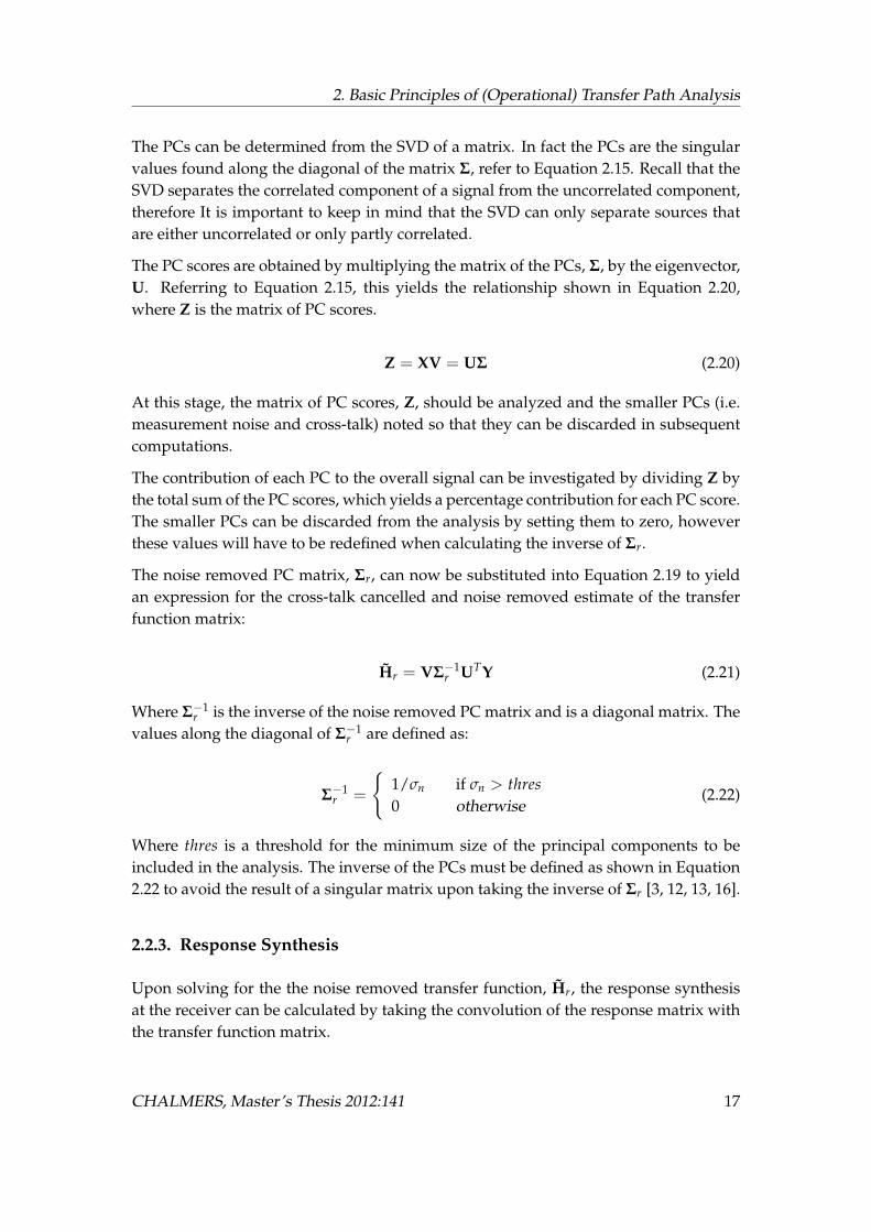
The PCs can be determined from the SVD of a matrix. In fact the PCs are the singularvalues found along the diagonal of the matrix S, refer to Equation 2.15. Recall that theSVD separates the correlated component of a signal from the uncorrelated component,therefore It is important to keep in mind that the SVD can only separate sources thatare either uncorrelated or only partly correlated.
The PC scores are obtained by multiplying the matrix of the PCs, S, by the eigenvector,U. Referring to Equation 2.15, this yields the relationship shown in Equation 2.20,where Z is the matrix of PC scores.
Z = XV = US (2.20)
At this stage, the matrix of PC scores, Z, should be analyzed and the smaller PCs (i.e.measurement noise and cross-talk) noted so that they can be discarded in subsequentcomputations.
The contribution of each PC to the overall signal can be investigated by dividing Z bythe total sum of the PC scores, which yields a percentage contribution for each PC score.The smaller PCs can be discarded from the analysis by setting them to zero, howeverthese values will have to be redefined when calculating the inverse of Sr.
The noise removed PC matrix, Sr, can now be substituted into Equation 2.19 to yieldan expression for the cross-talk cancelled and noise removed estimate of the transferfunction matrix:
Hr = VS�1r UTY (2.21)
Where S�1r is the inverse of the noise removed PC matrix and is a diagonal matrix. The
values along the diagonal of S�1r are defined as:
S�1r =
(1/sn if sn > thres0 otherwise
(2.22)
Where thres is a threshold for the minimum size of the principal components to beincluded in the analysis. The inverse of the PCs must be defined as shown in Equation2.22 to avoid the result of a singular matrix upon taking the inverse of Sr [3, 12, 13, 16].
2.2.3. Response Synthesis
Upon solving for the the noise removed transfer function, Hr, the response synthesisat the receiver can be calculated by taking the convolution of the response matrix withthe transfer function matrix.
CHALMERS, Master’s Thesis 2012:141 17
2.2. The Operational Transfer Path Analysis (OTPA) Method
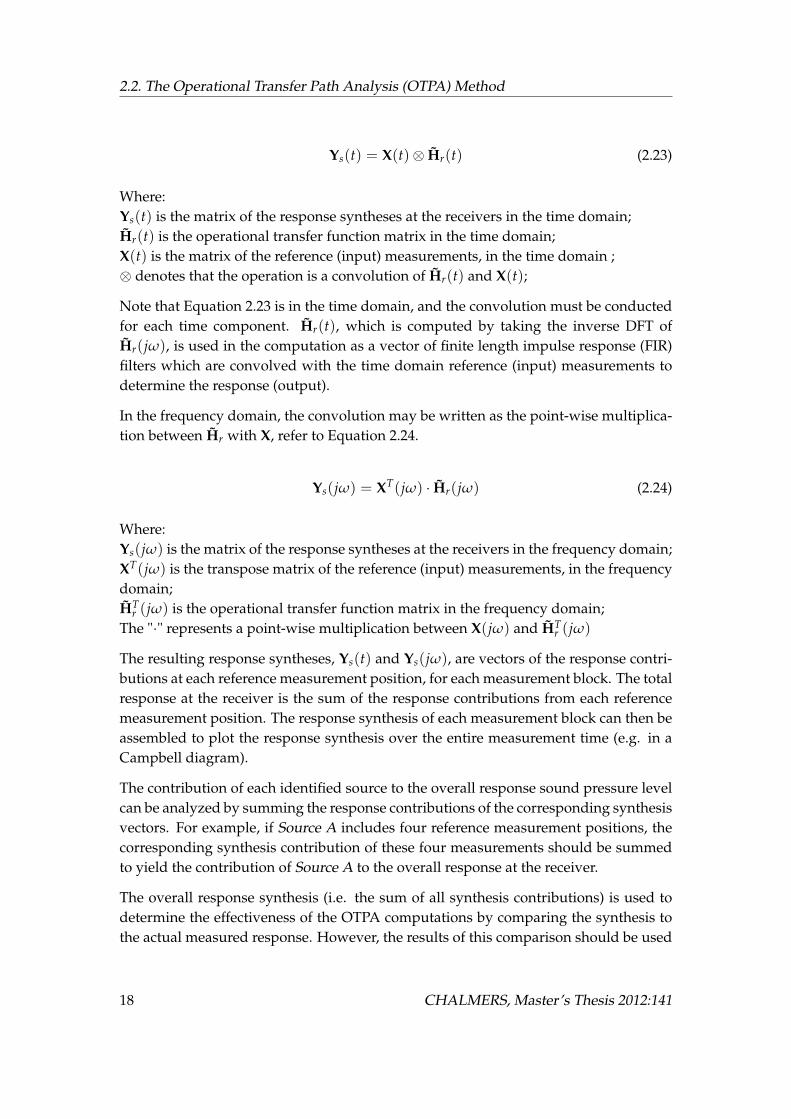
Ys(t) = X(t)⌦ Hr(t) (2.23)
Where:Ys(t) is the matrix of the response syntheses at the receivers in the time domain;Hr(t) is the operational transfer function matrix in the time domain;X(t) is the matrix of the reference (input) measurements, in the time domain ;⌦ denotes that the operation is a convolution of Hr(t) and X(t);
Note that Equation 2.23 is in the time domain, and the convolution must be conductedfor each time component. Hr(t), which is computed by taking the inverse DFT ofHr(jw), is used in the computation as a vector of finite length impulse response (FIR)filters which are convolved with the time domain reference (input) measurements todetermine the response (output).
In the frequency domain, the convolution may be written as the point-wise multiplica-tion between Hr with X, refer to Equation 2.24.
Ys(jw) = XT(jw) · Hr(jw) (2.24)
Where:Ys(jw) is the matrix of the response syntheses at the receivers in the frequency domain;XT(jw) is the transpose matrix of the reference (input) measurements, in the frequencydomain;HT
r (jw) is the operational transfer function matrix in the frequency domain;The "·" represents a point-wise multiplication between X(jw) and HT
r (jw)
The resulting response syntheses, Ys(t) and Ys(jw), are vectors of the response contri-butions at each reference measurement position, for each measurement block. The totalresponse at the receiver is the sum of the response contributions from each referencemeasurement position. The response synthesis of each measurement block can then beassembled to plot the response synthesis over the entire measurement time (e.g. in aCampbell diagram).
The contribution of each identified source to the overall response sound pressure levelcan be analyzed by summing the response contributions of the corresponding synthesisvectors. For example, if Source A includes four reference measurement positions, thecorresponding synthesis contribution of these four measurements should be summedto yield the contribution of Source A to the overall response at the receiver.
The overall response synthesis (i.e. the sum of all synthesis contributions) is used todetermine the effectiveness of the OTPA computations by comparing the synthesis tothe actual measured response. However, the results of this comparison should be used
18 CHALMERS, Master’s Thesis 2012:141

2. Basic Principles of (Operational) Transfer Path Analysis
with care - the overall response synthesis will almost always match the measured re-sponse at the receiver. This does not, however, necessarily mean that the calculatedcontributions are correct [24]. The limitations of the OTPA method are discussed inSection 2.2.4.
2.2.4. OTPA Limitations and Potential Sources of Error
The main characteristic of the OTPA method is that the resulting transfer functions arenot FRFs, but are analogous to transmissibilities. Therefore the transfer functions arespecifically related to the operational excitation signals used in the computation. Ifcertain modes are not excited by the excitation signals, these modes will not be iden-tified in the analysis. This fact is usually considered acceptable for the analysis of avehicle since the typical operational forces can be included in the analysis (e.g. idle,acceleration, coast-down), thus all relevant excitations are included.
A potential source of error in using the OTPA method stems from the fact that thereliability of the results is highly dependant on properly setting up the measurement.This is also true for the classical TPA method, however an error in identifying all ofthe significant sources/paths is apparent during analysis of the classical TPA results,whereas for OTPA it may not be so clear.
The reliability of the OTPA model is often checked by comparing the actual measuredresponse to the response synthesis. A common claim for its accuracy is based on thecomparison of the the sum of all source/path contributions to the actual measuredsignal. This comparison, however, does not prove that the individual source/path syn-thesis contributions are correct [14].
In fact, the overall response synthesis and the actual measured response will alwayshave very similar, if not matching, results. This occurs because similar measured inputsare used in the computation of the transfer function.
A literature review indicates that there are three critical elements that could lead toerroneous transfer path estimates [9, 10, 14, 24]:
1. Neglected sources/paths in the measurement setup.
2. Cross-coupling between input measurements (i.e. CTC is not able to separate thesources/paths).
3. Incorrect estimation of the transmissibilities (transfer paths).
The result of these three elements is that the source/path contribution calculation iserroneous, however, as stated earlier in this section, the overall response synthesis maystill appear to be correct (i.e. the overall response synthesis matches the measuredresponse). These elements are briefly discussed in the following.
CHALMERS, Master’s Thesis 2012:141 19

2.2. The Operational Transfer Path Analysis (OTPA) Method
Neglected sources/paths in the measurement setup
Neglected sources/paths can introduce errors particularly if they are correlated withthose included in the analysis, as its energy will be spread over to the other sources/-paths. Consequently, the overall response synthesis will still match the measured re-sponse – the synthesis contributions will be skewed to account for the energy of thesource/path contributions that were not included in the measurement setup.
If the neglected sources/paths are not correlated with those that are included in theanalysis, the error will show up in the overall response synthesis – it will not match themeasured response.
Cross-coupling between input measurements
Difficulties in the cross-talk cancellation using SVD and PCA arise when two or morestrong and highly coherent sources/paths exist for the system. The CTC technique isnot able to accurately separate two completely coherent sources/paths, and thereforethe results yield erroneous contribution estimates.
If there is cross-talk between non-coherent, or even partly coherent sources/paths, theCTC technique can be used successfully for source/path separation.
Incorrect estimation of transfer paths
The third critical element refers to the fact that the OTPA method relies on SVD andPCA in order to calculate the pseudo-inverse of the matrix of reference/input mea-surements. Because the pseudo-inverse calculation is an approximation, the resultsmay not be accurate.
Further, because the OTPA is based on a transmissibility, if all of the significant inputexcitations are not included in the analysis, the calculated transfer paths will be incor-rect. The potential for this error can be alleviated by including measurements for sev-eral operational conditions in the reference/input matrix (e.g. run-up and run-down atseveral gear positions).
20 CHALMERS, Master’s Thesis 2012:141

3. Implementation of OTPA and CTC
Based on the OTPA theory discussed in Section 2.2, an OTPA script has been imple-mented using MATLAB. The OTPA program flow is summarized in the following:
1. Load measurement data. If the data is in the time domain, transform the data tofrequency domain (i.e. DFT)1.
2. Assemble measurement data into reference matrix, X(jw) and response matrixY(jw).
3. SVD of matrix X(jw) into its principal components.4. PCA of matrix S, which consists of the PCs along its diagonal.5. Remove less important PCs (i.e. noise and cross-talk from the other source).6. Compute the pseudo-inverse of Xr(jw) – the noise removed and cross-talk can-
celled matrix of reference measurements.7. Calculate the cross-talk cancelled transfer function, Hr(jw).8. Load a separate set of input data, X so that the calculation of the response syn-
thesis is not circular logic (i.e. the same input data used to compute the transferfunction, is not used again to compute the response synthesis).
9. Calculate the response synthesis, Ys(jw), as well as the source contributions byadding up the relevant vectors of Ys(jw) (i.e. those that correspond to the source’sreference MPs).
10. Calculate the transfer function in the time domain, Hr(t), by taking the inverseDFT of Hr(jw).
11. Calculate the response synthesis in the time domain by convolving X(t) andHr(t).
A flow chart of the OTPA script organization is displayed in Figure 3.1.
1The virtual test setup, described in Chapter 4, is implemented in the frequency domain, thus signalprocessing to transform the signal from the time domain to the frequency domain is not required, andis not further discussed in this thesis.
21

Load Measurement Data X(jω) and Y(jω)
PCA
Compute X-1(jω) and Hr(jω) Inverse FFT of Hr(jω)
➔ Hr(t) [FIR Filter]
Loop for N Frequency
Components
Time Domain:Response Contribution Synthesis
Ys(t) = X(t)⊗Hr(t)
SVD of X(jω)
Frequency Domain:Response Contribution Synthesis
Ys(jω) = X(jω)!Hr(jω)
Load New Measurement Data X(jω)
Load New Measurement Data X(t)
Figure 3.1.: OTPA Program Flow Chart
22 CHALMERS, Master’s Thesis 2012:141

3. Implementation of OTPA and CTC
3.1. MATLAB Script: Description of Key Functions
A description of the key functions used in the OTPA implementation in MATLAB aredescribed in the following.
3.1.1. Singular Value Decomposition
The OTPA script is made fairly simple by using the embedded MATLAB function forthe singular value decomposition of the matrix X(jw). The command to compute theSVD is:
[U, S, V] = SVD(X) (3.1)
Where U and V are the eigenvector matrices and S is the matrix of singular values (i.e.principal components). Observe that in Equation 2.15, the matrix of singular values, S,is represented by S in the MATLAB script. Refer to Section 2.2.2 for the theory behindthe SVD computation.
The output of this function reveals the principal components and eigenvector matri-ces from which the principal component scores as well as cumulative contribution aredetermined, see Equation 2.20.
3.1.2. Principal Component Analysis and Cross-Talk Cancellation
There are several methods to conduct the PCA. Four of these methods are included inthe OTPA script, however, to maintain consistency, only one method is used for theanalyses. The PCA methods included in the script are described in the following:
The first option is to simply define the number of PCs that are to be included in theanalysis. For example, if that number is defined as two, the two highest ranked PCs areincluded in matrix S, and the rest are set to discarded (e.g. set to zero).
The second option, which is the method used for the analyses described in this thesisreport, is to define a threshold, as a percentage, for the minimum contribution of thePCs towards the total sum of the PC scores (i.e. towards the total contribution). Forexample, if a threshold of 5% is defined, any PCs that contribute 5% or less to theoverall contribution will be excluded.
The third option is to define a minimum cumulative contribution that the PCs includedin the analysis must meet. For example, if a cumulative contribution of 90% is defined,the highest ranked PCs are included in the analysis until the cumulative contributionis equal to 90%. Any left over PCs are set to zero, and thus discarded from the analysis.
CHALMERS, Master’s Thesis 2012:141 23

3.1. MATLAB Script: Description of Key Functions
The fourth option allows the user to simply identify the minimum magnitude of theprincipal components to be included in the the analysis (i.e. the minimum magnitudeof the values in S that are to be included).
3.1.3. Response Synthesis and Contribution Analysis
Once the transfer function, H, has been determined, the response synthesis is calculatedby a point-wise multiplication between X and H.
Y = X0. ⇤ H (3.2)
Where the matrix of input reference measurements, X is transposed so that the MPs aremultiplied by the corresponding transfer function for each measurement block. The re-sulting response matrix, Y, consists of the contribution to the total response from eachmeasurement position. Therefore, if a source includes two MPs, these two MPs must besummed to yield the contribution of that particular source. Similarly, the overall syn-thesis at a particular receiver is the sum of all the contributions of that correspondingvector in matrix Y.
Note that these functions are repeated for each frequency component (i.e. looped for Niterations, where N corresponds to the number of frequency components).
The full Matlab script for the OTPA program is included in Appendix A. Note thatthe included script is customized for the analyses included in this report. Further, theOTPA script has its limitations – as the number of sources/paths increases, it may be-come impractical to use the provided script.
24 CHALMERS, Master’s Thesis 2012:141

4. The Virtual Test Setup
A virtual test setup (VTS) has been created in order to study the OTPA method ina highly controlled environment. The VTS was chosen over a real test setup so thatall of the "measurement" parameters could be controlled. Further, the analysis resultsobtained using the VTS are not influenced by any unknown external sources of error.
The main objective of the study is to recreate the over-prediction of airborne sound andconsequently to determine if limitations and/or rules of thumb can be clearly definedfor the OTPA method in this frequency range.
4.1. Virtual Test Setup Layout
The virtual test setup has been created in order to address the hypotheses stated inSection 1.2.1. Although various scenarios are investigated, the basic VTS layout can bedescribed as two spherically radiating sources and one receiver position in a completelyfree-field environment. The two sources, Source A and Source B, can be moved awayfrom each other, while the distances from Source A to the receiver and Source B tothe receiver remains equal. Each source is "measured" by one reference MP for mostof the analyses, however, in some cases more than one reference MP is included. Thedistance between reference MPs and the source may be defined in the program, but itis generally at the same distance for most of the analyses. A schematic of the virtualtest setup is shown in Figure 4.1.
The VTS layout was implemented using MATLAB by defining the source, referenceand response positions as coordinates. The distances between points is then easilydetermined.
The MATLAB script used to define the layout is included in Appendix A.
4.2. Source Signals - Background Theory
The sources are defined so that all computations can be conducted in the frequencydomain – This is done for simplicity, since the OTPA analysis is generally conductedin the frequency domain (although it is sometimes conducted in the time domain [25]).
25

4.2. Source Signals - Background Theory
Response MP[P
Tot= P
A+P
B]
Source A Source B
rAB
rA= r
B
Source A Source B
Ref. MPA
[PTot
= PA+P
B]
Ref. MPB
[PTot
= PA+P
B]
Cross-Talk
!A
16
!A
"#
Figure 4.1.: Virtual Test Setup Schematic
The two sources are modelled as radiating spherical sources of radius a and b (wherea = b). The sound pressure level at a radius rA from the Source A is described byEquation 4.1.
pA(r, w) = vAjwr0a2
1 + jkAae�jkA(rA�a)
rA(4.1)
Where:vA is the vibrational velocity of the surface of Source A at frequency w;jw denotes the complex angular frequency;r0 is the density of the surrounding medium (i.e. air). kA is the wave number, whereka = w/c = 2p/l, and c is the speed of sound;rA is the distance from Source A to the MP;a is the radius of the spherical source.
The resulting sound pressure level at the reference and response measurement posi-
26 CHALMERS, Master’s Thesis 2012:141

4. The Virtual Test Setup
tions can then be described as the vector addition of the contribution of the two sources,as shown in Equation 4.2 [2, 4].
ptotal(r, w) =
"vA
jwr0a2
1 + jkAae�jkA(rA�a)
rA+ vB
jwr0b2
1 + jkBbe�jkB(rB�b)
rB
#(4.2)
The MATLAB script for the computation of the source signal and resulting sound pres-sure levels at the receiver MPs and response MP is included in Appendix A.
4.3. VTS and OTPA Parameters
4.3.1. VTS Paramaters
The parameters used in the VTS were kept to reasonable values. For example, the sizeof the vibrating spheres, that is, the radii for Sources A and B are defined as lA
40 (at 25Hz this is 0.35 m), which is a fairly close approximation of the size of the engine of avehicle.
The reference MPs for the sources are positioned at a radius of lA16 from the centre of the
sources. At 25 Hz, this distance puts the MPs at a distance of 0.5 m from the surface ofthe sources. Again, this distance is realistic when compared to microphone placementfor actual OTPA measurement setups.
The response MP is equidistant from both sources, with the right-angle distance of lApp
.This distance was chosen simply so that the distance is not an integer multiple of lA,as using an integer multiple could lead to unique results specific to that position.
The vibration velocity of the sphere’s surface is arbitrary, and is defined simply to yielda good scale for the plots. The actual magnitude of the source is not of importance sinceonly the relative values are of interest in this study. Both sources are in phase, unless aphase shift is specifically mentioned in the analysis.
The OTPA analysis calls for several measurement blocks of data – this is treated by sim-ply looping the VTS output so that the reference matrix includes several measurementblocks with the same response. This is done to keep the analysis of the OTPA simple.
Noise is introduced to the signals by adding a random sound pressure to the VTSthroughout the full frequency range of interest (up to 200 Hz). The random noise isdifferent for each "measurement block".
Some of the input variables for the sources may vary depending on the analysis, how-ever any significant changes are noted in the discussion for each individual analysis.
CHALMERS, Master’s Thesis 2012:141 27

4.3. VTS and OTPA Parameters
4.3.2. OTPA Parameters
The input parameters for the OTPA relate to the principal component analysis, whichis used for the cross-talk cancellation. The VTS is quite simple, such that with onlytwo reference MPs (one for each source), at any frequency the maximum number ofPCs would be two. For the sake of consistency between the analyses, the PCA tech-nique used is a minimum threshold towards the total contribution at each frequencycomponent, which was set to 5% for all analyses (unless otherwise stated).
The MATLAB script for analyses are included in Appendix A.
28 CHALMERS, Master’s Thesis 2012:141

5. Analysis
5.1. Analysis Outline
The study of the OTPA method is set up to first validate both the OTPA and VTS pro-grams, and then to investigate the hypotheses discussed in Section 1.2.1.
The validation of the OTPA program is conducted by examining a simple case consist-ing of two airborne sources radiating random noise throughout the frequency range ofinterest, as well as a dominant tone. The effects of varying the PCA threshold value onthe overall source synthesis are also examined.
Next, two simple cases consisting of two airborne sources and one receiver are studied.These cases are used to study the effects of cross-talk between reference MPs.
The VTS is then slightly modified so that it includes one airborne sound path and onestructure-borne sound path. This setup is designed to be a simplified setup of the trac-tor OTPA case study (refer to Section 1.1). Furthermore, a "falsely identified" airbornesource is also included in this VTS – this is analogous to including the tire airbornesound reference MPs during the neutral OTPA of the tractor (i.e. the tires are not asignificant noise source when the vehicle is stationary).
Finally, because the number of reference MPs included in the actual measurement ap-peared to have an effect on the tractor OTPA results1, the effect of the number of refer-ence MPs included in the analysis is also studied.
In summary, the OTPA study using the VTS is structured as follows:
1. Validation of the OTPA MATLAB program: Noise removal using PCA.2. The effect of varying distance between two fully correlated airborne sources on
the contribution prediction results.3. The effect of varying the distance between two fully uncorrelated airborne sources
on the contribution prediction results.4. The effect of including a structure-borne source/path which is correlated with
the airborne source as well as a second "falsely identified" airborne source (i.e. asource that is not radiating sound) on the contribution prediction results.
1Recall that the calculated source contribution was different for the analysis with twelve airborne refer-ence MPs when compared to the case with six airborne reference MPs
29

5.1. Analysis Outline
5. The effect of varying the number of airborne source reference MPs on the contri-bution prediction results.
30 CHALMERS, Master’s Thesis 2012:141
5. Analysis
5.2. OTPA Validation: CTC and Noise Removal Using PCA
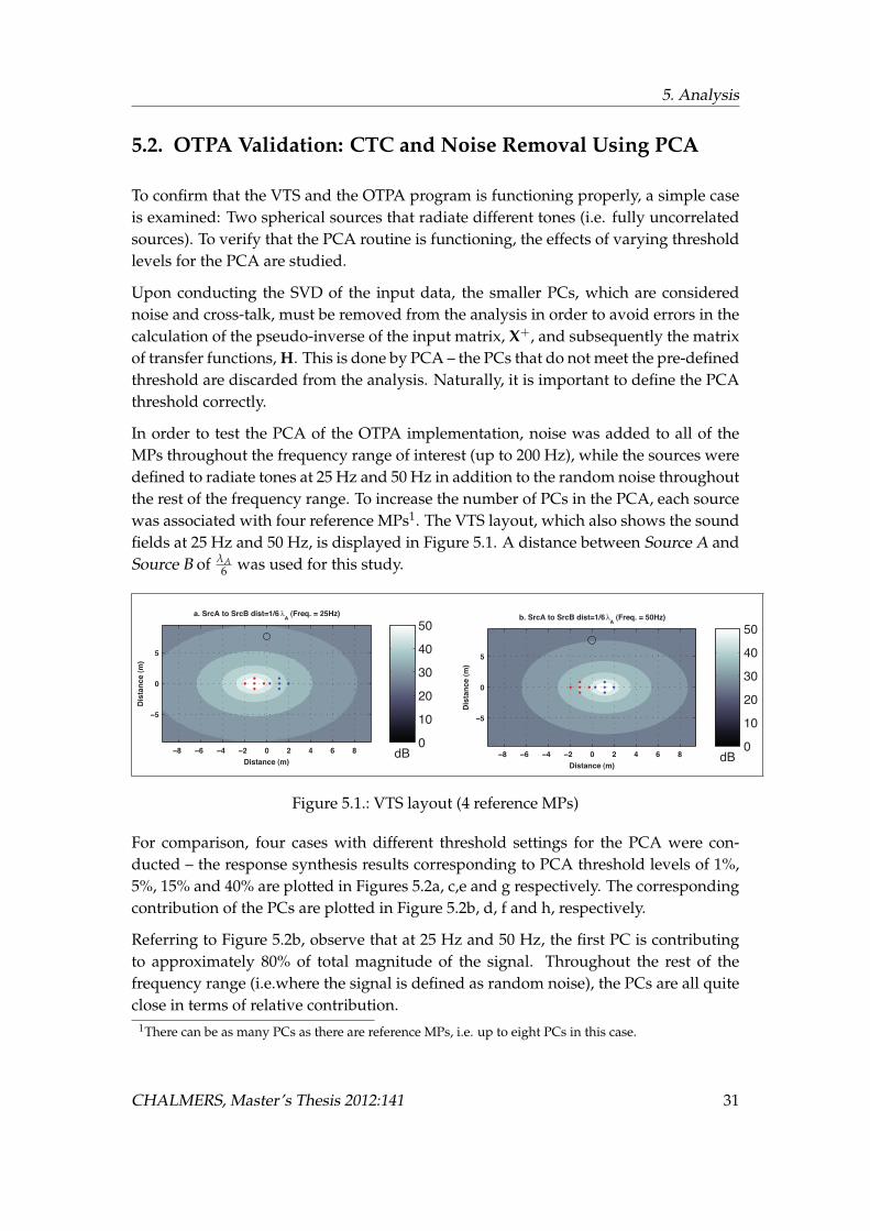
To confirm that the VTS and the OTPA program is functioning properly, a simple caseis examined: Two spherical sources that radiate different tones (i.e. fully uncorrelatedsources). To verify that the PCA routine is functioning, the effects of varying thresholdlevels for the PCA are studied.
Upon conducting the SVD of the input data, the smaller PCs, which are considerednoise and cross-talk, must be removed from the analysis in order to avoid errors in thecalculation of the pseudo-inverse of the input matrix, X+, and subsequently the matrixof transfer functions, H. This is done by PCA – the PCs that do not meet the pre-definedthreshold are discarded from the analysis. Naturally, it is important to define the PCAthreshold correctly.
In order to test the PCA of the OTPA implementation, noise was added to all of theMPs throughout the frequency range of interest (up to 200 Hz), while the sources weredefined to radiate tones at 25 Hz and 50 Hz in addition to the random noise throughoutthe rest of the frequency range. To increase the number of PCs in the PCA, each sourcewas associated with four reference MPs1. The VTS layout, which also shows the soundfields at 25 Hz and 50 Hz, is displayed in Figure 5.1. A distance between Source A andSource B of lA
6 was used for this study.
Distance (m)
Dis
tan
ce
(m
)
a. SrcA to SrcB dist=1/6 !A (Freq. = 25Hz)
!8 !6 !4 !2 0 2 4 6 8
!5
0
5
dB0
10
20
30
40
50
Distance (m)
Dis
tan
ce
(m
)
b. SrcA to SrcB dist=1/6 !A (Freq. = 50Hz)
!8 !6 !4 !2 0 2 4 6 8
!5
0
5
dB0
10
20
30
40
50
Figure 5.1.: VTS layout (4 reference MPs)
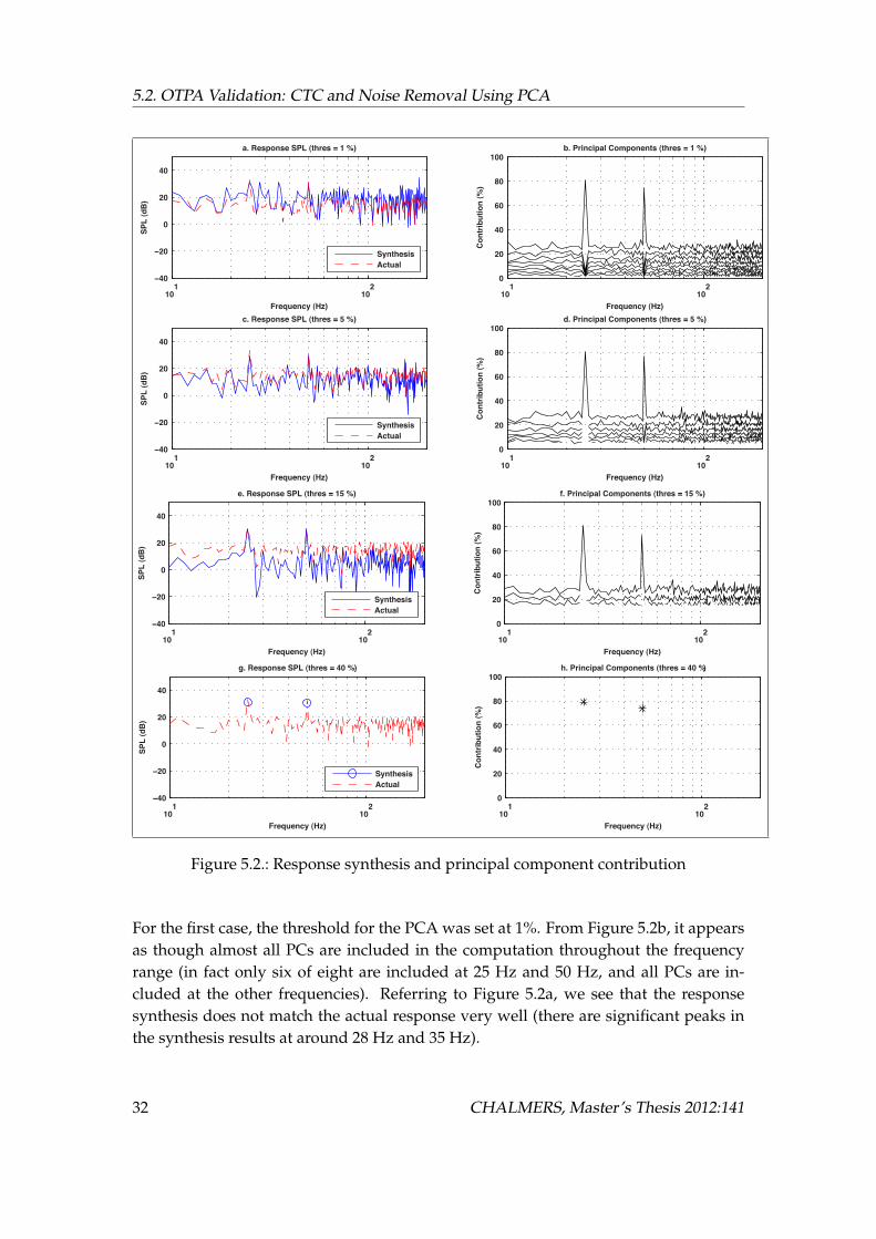
For comparison, four cases with different threshold settings for the PCA were con-ducted – the response synthesis results corresponding to PCA threshold levels of 1%,5%, 15% and 40% are plotted in Figures 5.2a, c,e and g respectively. The correspondingcontribution of the PCs are plotted in Figure 5.2b, d, f and h, respectively.
Referring to Figure 5.2b, observe that at 25 Hz and 50 Hz, the first PC is contributingto approximately 80% of total magnitude of the signal. Throughout the rest of thefrequency range (i.e.where the signal is defined as random noise), the PCs are all quiteclose in terms of relative contribution.
1There can be as many PCs as there are reference MPs, i.e. up to eight PCs in this case.
CHALMERS, Master’s Thesis 2012:141 31
5.2. OTPA Validation: CTC and Noise Removal Using PCA
101
102
!40
!20
0
20
40
a. Response SPL (thres = 1 %)
Frequency (Hz)
SP
L (
dB
)
Synthesis
Actual
101
102
0
20
40
60
80
100b. Principal Components (thres = 1 %)
Co
ntr
ibu
tio
n (
%)
Frequency (Hz)
101
102
!40
!20
0
20
40
c. Response SPL (thres = 5 %)
Frequency (Hz)
SP
L (
dB
)
Synthesis
Actual
101
102
0
20
40
60
80
100d. Principal Components (thres = 5 %)
Co
ntr
ibu
tio
n (
%)
Frequency (Hz)
101
102
!40
!20
0
20
40
e. Response SPL (thres = 15 %)
Frequency (Hz)
SP
L (
dB
)
Synthesis
Actual
101
102
0
20
40
60
80
100f. Principal Components (thres = 15 %)
Co
ntr
ibu
tio
n (
%)
Frequency (Hz)
101
102
!40
!20
0
20
40
g. Response SPL (thres = 40 %)
Frequency (Hz)
SP
L (
dB
)
Synthesis
Actual
101
102
0
20
40
60
80
100h. Principal Components (thres = 40 %)
Co
ntr
ibu
tio
n (
%)
Frequency (Hz)
Figure 5.2.: Response synthesis and principal component contribution
For the first case, the threshold for the PCA was set at 1%. From Figure 5.2b, it appearsas though almost all PCs are included in the computation throughout the frequencyrange (in fact only six of eight are included at 25 Hz and 50 Hz, and all PCs are in-cluded at the other frequencies). Referring to Figure 5.2a, we see that the responsesynthesis does not match the actual response very well (there are significant peaks inthe synthesis results at around 28 Hz and 35 Hz).
32 CHALMERS, Master’s Thesis 2012:141
5. Analysis
Increasing the threshold to 5% yields the response synthesis displayed in Figure 5.2c.For this case, we see from Figure 5.2d that only two or three PCs are included in thecomputation at the radiated tones (25 Hz and 50 Hz), and six or seven PCs are includedfor the rest of the frequency components. Note that with only a slight increase in thethreshold level, the response synthesis matches the actual response quite accurately.The response synthesis has been improved because the small PCs have now been dis-carded – thus the uncorrelated noise component (the noise) has been removed from theanalysis, which in turn reduces the potential error in the computation of the pseudo-inverse of the input matrix, and subsequently the transfer function.
For the next case, the threshold was again increased slightly, to 15%. Referring to Figure5.2f, we see that only the first PCs remain at 25Hz and 50Hz, while throughout therest of the frequency range two to three PCs are included. Looking at the responsesynthesis, refer to Figure 5.2e, we see that although the tones at 25Hz and 50Hz matchwith the actual response, the synthesis throughout the rest of the frequency range doesnot agree very well.
Upon examination of the PCs that are included in the analysis, we see that the two orthree remaining PCs only represent approximately 45% of the total signal – thus theresponse synthesis is an under-prediction of the actual response.
If it is desired to remove the noise completely while keeping the dominant tones inthe analysis, a higher threshold level could be used. This case was tested by setting athreshold level of 40% for the analysis. Referring to Figure 5.2h, we observe that onlythe first PCs at 25Hz and 50Hz remain – all other PCs have been discarded from theanalysis. Therefore, the resulting response synthesis, displayed in Figure 5.2g, onlyincludes the tones at 25 Hz and 50 Hz, as expected.
The results of this study confirm that the PCA of the OTPA program is functioning asexpected – thus validating the implementation. Also, the results show that the PCA isa useful tool to identify the strong contributions in a signal – however, it is importantto appropriately set the threshold for the PCA in order to yield accurate results.
5.3. OTPA of Two Airborne Noise Sources
The following case studies consist of two spherical airborne sources, labeled SourceA and Source B, which have a certain surface vibration that causes a radiated soundpower at a specified tone. In the first case, two correlated sources are studied, and inthe second case two uncorrelated sources are studied.
CHALMERS, Master’s Thesis 2012:141 33

5.3. OTPA of Two Airborne Noise Sources
5.3.1. Varying Distance Between Two Correlated Sources
This case study consists of two airborne sources, labeled Source A and Source B, thatradiate sound power at a single tone, 25 Hz. Both sources are the same size, have thesame amplitude, and are in phase. The response MP (i.e. the receiver) is equidistantfrom both sources, with an initial distance of lAp
p.
A plot of the VTS layout that includes the sound field is displayed in Figure 5.3. Notethat the response MP is denoted by a circle at the top of the figures, while the sourcesare in the centre; Source A is moved to the left, and Source B is moved to the right. Eachsource is represented by one reference MP – located to the left of Source A, and to theright of Source B.
Distance (m)
Dis
tan
ce (
m)
a. SrcA to SrcB dist=0 !A (Freq.=25Hz)
!8 !6 !4 !2 0 2 4 6 8
!5
0
5
dB0
10
20
30
40
50
Distance (m)
Dis
tan
ce (
m)
b. SrcA to SrcB dist=1/8 !A (Freq. = 25Hz)
!8 !6 !4 !2 0 2 4 6 8
!5
0
5
dB0
10
20
30
40
50
Distance (m)
Dis
tan
ce (
m)
c. SrcA to SrcB dist=1/6 !A (Freq. = 25Hz)
!8 !6 !4 !2 0 2 4 6 8
!5
0
5
dB0
10
20
30
40
50
Distance (m)
Dis
tan
ce (
m)
d. SrcA to SrcB dist=1/4 !A (Freq. = 25Hz)
!8 !6 !4 !2 0 2 4 6 8
!5
0
5
dB0
10
20
30
40
50
Distance (m)
Dis
tan
ce (
m)
e. SrcA to SrcB dist=1/2 !A (Freq. = 25Hz)
!8 !6 !4 !2 0 2 4 6 8
!5
0
5
dB0
10
20
30
40
50
Distance (m)
Dis
tan
ce (
m)
f. SrcA to SrcB dist= !A (Freq.=25Hz)
!8 !6 !4 !2 0 2 4 6 8
!5
0
5
dB0
10
20
30
40
50
Figure 5.3.: Sound field – correlated sources (QA = QB, fA = fB)
Referring to Figure 5.3a, where the sources are at the exact same location, the soundfield appears as if there is only one source, which is as expected for two fully coherentsources at exactly the same location (i.e. this can be considered a single source). Once
34 CHALMERS, Master’s Thesis 2012:141

5. Analysis
the sources are moved apart, refer to Figures 5.3b-f, the interaction between the sourcescan be seen, resulting in an interference pattern in the sound field.
Total Source A Source B0
5
10
15
20
25
30
35
40
45
50
SP
L (
dB
)
a. SrcA to Src B dist=0 !A (Freq. = 25Hz)
Actual Calculated
Total Source A Source B0
5
10
15
20
25
30
35
40
45
50
SP
L (
dB
)
b. SrcA to SrcB dist=1/8 !A (Freq. = 25Hz)
Actual Calculated
Total Source A Source B0
5
10
15
20
25
30
35
40
45
50
SP
L (
dB
)
c. SrcA to SrcB dist=1/6 !A (Freq. = 25Hz)
Actual Calculated
Total Source A Source B0
5
10
15
20
25
30
35
40
45
50
SP
L (
dB
)
d. SrcA to SrcB dist=1/4 !A (Freq. = 25Hz)
Actual Calculated
Total Source A Source B0
5
10
15
20
25
30
35
40
45
50
SP
L (
dB
)
e. SrcA to SrcB dist=1/2 !A (Freq. = 25Hz)
Actual Calculated
Total Source A Source B0
5
10
15
20
25
30
35
40
45
50
SP
L (
dB
)
f. SrcA to Src B dist= !A (Freq. = 25Hz)
Actual Calculated
Figure 5.4.: Source contribution – correlated sources (QA = QB, fA = fB)
From Figure 5.4, note that the contributions of Source A and Source B are the same forall configurations, and that the calculated source contribution agrees with the actualsource contributions. The results are as expected, however, this case may be consid-ered as trivial in the sense that cross-talk between the reference MPs would not beidentifiable with two identical (fully correlated) sources.
Therefore, a supplementary study, similar to the one just described, was setup for fur-ther investigation of the OTPA method. In this study, the amplitude of Source B washalved, so that QA = 2QB. The results are displayed in Figures 5.5 and 5.6.
Referring to the source contribution plots in Figure 5.6, observe that, as expected, whenthe sources are at the same position (Figure 5.6a), the OTPA algorithm can not distin-guish between the sources, thus, the results indicate that each source exhibits an equalcontribution towards the overall sound level at the response position.
CHALMERS, Master’s Thesis 2012:141 35

5.3. OTPA of Two Airborne Noise Sources
Distance (m)
Dis
tan
ce (
m)
a. SrcA to SrcB dist=0 !A (Freq.=25Hz)
!8 !6 !4 !2 0 2 4 6 8
!5
0
5
dB0
10
20
30
40
50
Distance (m)
Dis
tan
ce (
m)
b. SrcA to SrcB dist=1/8 !A (Freq. = 25Hz)
!8 !6 !4 !2 0 2 4 6 8
!5
0
5
dB0
10
20
30
40
50
Distance (m)
Dis
tan
ce (
m)
c. SrcA to SrcB dist=1/6 !A (Freq. = 25Hz)
!8 !6 !4 !2 0 2 4 6 8
!5
0
5
dB0
10
20
30
40
50
Distance (m)D
ista
nce (
m)
d. SrcA to SrcB dist=1/4 !A (Freq. = 25Hz)
!8 !6 !4 !2 0 2 4 6 8
!5
0
5
dB0
10
20
30
40
50
Distance (m)
Dis
tan
ce (
m)
e. SrcA to SrcB dist=1/2 !A (Freq. = 25Hz)
!8 !6 !4 !2 0 2 4 6 8
!5
0
5
dB0
10
20
30
40
50
Distance (m)
Dis
tan
ce (
m)
f. SrcA to SrcB dist= !A (Freq.=25Hz)
!8 !6 !4 !2 0 2 4 6 8
!5
0
5
dB0
10
20
30
40
50
Figure 5.5.: Sound field – correlated sources (QA = 2QB, fA = fB)
Once the sources are moved apart, the overall response synthesis remains accurate,however, the source contribution estimates are not accurate – the stronger source strengthis over estimated, and the weaker source is under estimated. Referring to Figure 5.6c-f,note that as the sources are moved further apart, the cross-talk between the referenceMPs is reduced and the source contribution estimates begin to agree more with theactual source contributions (although the results remain biased towards the strongersource). At a distance of lA
4 , the source contribution estimate is accurate to within afew dB (refer to Figure 5.6d). The source contribution estimate is accurate only becauseof the reduction in cross-talk, since the amplitude of the cross-talk from Source A is re-duced by 6 dB for each doubling of distance. Note that the calculated total contributionmatches the actual total contribution for all cases.
This result indicates that the reference MPs should be placed as close as possible to thesource – thus improving the signal-to-noise ratio (i.e. reducing the effects of cross-talk)and improving the calculated results.
36 CHALMERS, Master’s Thesis 2012:141

5. Analysis
Total Source A Source B0
5
10
15
20
25
30
35
40
45
50
SP
L (
dB
)
a. SrcA to Src B dist=0 !A (Freq. = 25Hz)
Actual Calculated
Total Source A Source B0
5
10
15
20
25
30
35
40
45
50
SP
L (
dB
)
b. SrcA to SrcB dist=1/8 !A (Freq. = 25Hz)
Actual Calculated
Total Source A Source B0
5
10
15
20
25
30
35
40
45
50
SP
L (
dB
)
c. SrcA to SrcB dist=1/6 !A (Freq. = 25Hz)
Actual Calculated
Total Source A Source B0
5
10
15
20
25
30
35
40
45
50
SP
L (
dB
)
d. SrcA to SrcB dist=1/4 !A (Freq. = 25Hz)
Actual Calculated
Total Source A Source B0
5
10
15
20
25
30
35
40
45
50
SP
L (
dB
)
e. SrcA to SrcB dist=1/2 !A (Freq. = 25Hz)
Actual Calculated
Total Source A Source B0
5
10
15
20
25
30
35
40
45
50
SP
L (
dB
)
f. SrcA to Src B dist= !A (Freq. = 25Hz)
Actual Calculated
Figure 5.6.: Source contribution – correlated sources (QA = 2QB, fA = fB)
Even when the two sources are very close (refer to Figure 5.6b), the conclusions thatwould be drawn from the OTPA results are useful – although the calculated sourcecontribution is not accurate (the synthesized source contribution deviates from the ac-tual contribution by approximately 3 dB for Source A and by approximately 18 dB forSource B), the results clearly indicate which source is the major contributor to the over-all sound level at the response position1.
1The CTC is not effective for fully correlated data, therefore it is expected that the same conclusionswould be drawn from the unprocessed data of the sound level measurements.
CHALMERS, Master’s Thesis 2012:141 37

5.3. OTPA of Two Airborne Noise Sources
5.3.2. Varying Distance Between Two Uncorrelated Sources
This case study involves two spherical sources – Source A and Source B, which radiatedifferent tones, 25 Hz and 50 Hz, respectively, at approximately the same amplitude.This scenario represents two uncorrelated sources, and therefore there should be nointerference in the discrete sound fields at these tones. Referring to the plots of thesound fields, shown in Figures 5.7 and 5.8, the results are as expected.
Distance (m)
Dis
tan
ce (
m)
a. SrcA to SrcB dist=0 !A (Freq.=25Hz)
!8 !6 !4 !2 0 2 4 6 8
!5
0
5
dB0
10
20
30
40
50
Distance (m)
Dis
tan
ce (
m)
b. SrcA to SrcB dist=1/8 !A (Freq. = 25Hz)
!8 !6 !4 !2 0 2 4 6 8
!5
0
5
dB0
10
20
30
40
50
Distance (m)
Dis
tan
ce (
m)
c. SrcA to SrcB dist=1/6 !A (Freq. = 25Hz)
!8 !6 !4 !2 0 2 4 6 8
!5
0
5
dB0
10
20
30
40
50
Distance (m)
Dis
tan
ce (
m)
d. SrcA to SrcB dist=1/4 !A (Freq. = 25Hz)
!8 !6 !4 !2 0 2 4 6 8
!5
0
5
dB0
10
20
30
40
50
Distance (m)
Dis
tan
ce (
m)
e. SrcA to SrcB dist=1/2 !A (Freq. = 25Hz)
!8 !6 !4 !2 0 2 4 6 8
!5
0
5
dB0
10
20
30
40
50
Distance (m)
Dis
tan
ce (
m)
f. SrcA to SrcB dist= !A (Freq.=25Hz)
!8 !6 !4 !2 0 2 4 6 8
!5
0
5
dB0
10
20
30
40
50
Figure 5.7.: Sound field at fA – uncorrelated sources ( fA 6= fB)
The calculated source contributions are included in Figures 5.9 and 5.10. Note that thesource contribution results are similar to the case with two correlated sources – Thatis to say that when both sources are at the same location (and therefore the referenceMPs are equidistant from the radiating source), the contribution synthesis indicatesthat both sources are contributing equally to the overall sound level at the responseposition. This, of course, is incorrect, however, as the distance between the two sourcesis increased, the response synthesis becomes increasingly accurate. Note that at a sep-aration distance of only 1/8lA (refer to Figures 5.9a and 5.10a), the response synthesis
38 CHALMERS, Master’s Thesis 2012:141

5. Analysis
Distance (m)
Dis
tan
ce (
m)
a. SrcA to SrcB dist=0 !A (Freq. = 50Hz)
!8 !6 !4 !2 0 2 4 6 8
!5
0
5
dB0
10
20
30
40
50
Distance (m)
Dis
tan
ce (
m)
b. SrcA to SrcB dist=1/8 !A (Freq. = 50Hz)
!8 !6 !4 !2 0 2 4 6 8
!5
0
5
dB0
10
20
30
40
50
Distance (m)
Dis
tan
ce (
m)
c. SrcA to SrcB dist=1/6 !A (Freq. = 50Hz)
!8 !6 !4 !2 0 2 4 6 8
!5
0
5
dB0
10
20
30
40
50
Distance (m)D
ista
nce (
m)
d. SrcA to SrcB dist=1/4 !A (Freq. = 50Hz)
!8 !6 !4 !2 0 2 4 6 8
!5
0
5
dB0
10
20
30
40
50
Distance (m)
Dis
tan
ce (
m)
e. SrcA to SrcB dist=1/2 !A (Freq. = 50Hz)
!8 !6 !4 !2 0 2 4 6 8
!5
0
5
dB0
10
20
30
40
50
Distance (m)
Dis
tan
ce (
m)
f. SrcA to SrcB dist= !A (Freq.=25Hz)
!8 !6 !4 !2 0 2 4 6 8
!5
0
5
dB0
10
20
30
40
50
Figure 5.8.: Sound field at fB – uncorrelated sources ( fA 6= fB)
is already fairly accurate.
Cross-referencing the sound field plots (Figures 5.7 and 5.8) with the source contribu-tion prediction results (Figures 5.9 and 5.10), we see that the incorrect contribution issimply related to the amplitude of the cross-talk at each particular distance.
Because the sources are only radiating a single tone, the reference MPs, regardless of thesource, pick up this signal – when introduced into the OTPA, this is of course assumedto be coming from the source that the reference MP is assigned to. Further, the CTCalgorithm yields a very strong first principal component which accounts for the themajority of the contribution towards the total sound pressure level at the response MP.
This case is analogous to a system which has two correlated sources as input to theOTPA algorithm. Thus, it is not possible to effectively cancel the cross-talk. To eliminatethe cross-talk, one possibility is to filter the measurement data, however this wouldrequire more information about the radiated sound from sources.
CHALMERS, Master’s Thesis 2012:141 39

5.3. OTPA of Two Airborne Noise Sources
Total Source A Source B0
5
10
15
20
25
30
35
40
45
50
SP
L (
dB
)
a. SrcA to Src B dist=0 !A (Freq. = 25Hz)
Actual Calculated
Total Source A Source B0
5
10
15
20
25
30
35
40
45
50
SP
L (
dB
)
b. SrcA to SrcB dist=1/8 !A (Freq. = 25Hz)
Actual Calculated
Total Source A Source B0
5
10
15
20
25
30
35
40
45
50
SP
L (
dB
)
c. SrcA to SrcB dist=1/6 !A (Freq. = 25Hz)
Actual Calculated
Total Source A Source B0
5
10
15
20
25
30
35
40
45
50
SP
L (
dB
)
d. SrcA to SrcB dist=1/4 !A (Freq. = 25Hz)
Actual Calculated
Total Source A Source B0
5
10
15
20
25
30
35
40
45
50
SP
L (
dB
)
e. SrcA to SrcB dist=1/2 !A (Freq. = 25Hz)
Actual Calculated
Total Source A Source B0
5
10
15
20
25
30
35
40
45
50
SP
L (
dB
)
f. SrcA to Src B dist= !A (Freq. = 25Hz)
Actual Calculated
Figure 5.9.: Source contribution at fA – uncorrelated sources ( fA 6= fB)
Although it has been established that some errors may arise if airborne sources arewithin a close proximity, it has been shown that even at very close distances (e.g. Fig-ures 5.9b and 5.10b), the results do give an accurate indication of which source is themain contributor. The analysis of these results could therefore lead to the correct strat-egy for any noise attenuation measures.
40 CHALMERS, Master’s Thesis 2012:141

5. Analysis
Total Source A Source B0
5
10
15
20
25
30
35
40
45
50
SP
L (
dB
)
a. SrcA to SrcB dist= 0 !A (Freq. = 50Hz)
Actual Calculated
Total Source A Source B0
5
10
15
20
25
30
35
40
45
50
SP
L (
dB
)
b. SrcA to SrcB dist=1/8 !A (Freq. = 50Hz)
Actual Calculated
Total Source A Source B0
5
10
15
20
25
30
35
40
45
50
SP
L (
dB
)
c. SrcA to SrcB dist=1/6 !A (Freq. = 50Hz)
Actual Calculated
Total Source A Source B0
5
10
15
20
25
30
35
40
45
50
SP
L (
dB
)
d. SrcA to SrcB dist=1/4 !A (Freq. = 50Hz)
Actual Calculated
Total Source A Source B0
5
10
15
20
25
30
35
40
45
50
SP
L (
dB
)
e. SrcA to SrcB dist=1/2 !A (Freq. = 50Hz)
Actual Calculated
Total Source A Source B0
5
10
15
20
25
30
35
40
45
50
SP
L (
dB
)
f. SrcA to Src B dist= !A (Freq. = 50Hz)
Actual Calculated
Figure 5.10.: Source contribution at fB – unorrelated sources ( fA 6= fB)
CHALMERS, Master’s Thesis 2012:141 41

5.3. OTPA of Two Airborne Noise Sources
5.3.3. Discussion and Summary of Results
The results of the two case studies presented in this sub-section lead to the followingconclusions:
• The sound field behaves according to what is expected, therefore the VTS imple-mentation is considered to be valid.
• The results of the case study with two correlated sources (i.e. the same frequencyand phase for Source A and Source B) indicate that the reference MPs must mainlymeasure the noise radiated from the source for which they are assigned (i.e. goodsignal to noise ratio) in order for the OTPA to compute an accurate source con-tribution. Further, the results indicate that for two strongly correlated sources/-paths, the source contribution results will likely yield an over-estimation of thestronger source strength, and under estimation of the weaker source strength.
• The results of the case study with two uncorrelated sources (i.e. different tonesfor Source A and Source B) indicate that the contribution analysis results could bemisleading if there is strong cross-talk to a reference MP for which its source is notradiating sound at this frequency (since the cross-talk would be correlated withthe other source). However, at a certain signal to noise ratio, the results indicatewhich source is the greatest contributor, thus leading to a correct conclusion.
42 CHALMERS, Master’s Thesis 2012:141

5. Analysis
5.4. OTPA of Correlated Structure-Borne and Airborne NoiseSources
Recall the tractor OTPA case study presented in Section 1.1 as the background to thisthesis. The OTPA consisted of several reference MPs, both for airborne sources (us-ing microphones) and for structure-borne sources (using accelerometers). The over-prediction of the airborne sound contribution (and under-prediction of the structure-borne sound contribution) was corrected by excluding data from the six non-criticalairborne MPs from the analysis.
In an attempt to recreate the over-prediction of the airborne sound contribution, theVTS was slightly modified by including one airborne sound (ABS) source/path andone structure-borne sound (SBS) source/path.
Recall from Section 2.2.2 that if an OTPA measurement setup includes mixed units,such as sound pressure (Pa) and vibration (e.g. acceleration, m/s2), the units mustbe normalized prior to the computations. In the VTS, the simulated reference and re-sponse data is normalized by scaling the SBS to be consistent with the ABS. To preservea simple model, the SBS path is assumed to be correlated with the ABS path such thatthe two paths comprise of the same normalized amplitude and phase contribution atboth the reference MP and the response MP.
5.4.1. Effects of Varying Distance of Additional Airborne Source MPs
This first simulation consists of a simplified setup of the case study presented in Section1.1. The OTPA is conducted on a VTS that includes one ABS path and one SBS path.Additionally, a falsely identified ABS source is also included in the model – that is tosay, an ABS source that does not radiate sound is included, simulating, for example,the tire reference MPs during a neutral run-up measurement.
Two primary reference MPs are used for the identified paths – one for the SBS path andone for the actual ABS path. An additional ABS reference MP is included in the modelat varying distance from the airborne source. This additional reference MP representsthe falsely identified ABS source. Thus, a total of three reference MPs (two for ABSand one for SBS) and one response MP are included in the analysis. The VTS layout isdisplayed along with the sound field in Figure 5.11.
The actual and calculated source contributions at the response position are displayedin Figure 5.12. Referring to Figure 5.12a, observe that there is an over-prediction ofthe ABS, and under-prediction of SBS, while the calculated total contribution agreeswith the actual contribution. This result coincides with the OTPA results for the tractorOTPA case study.
CHALMERS, Master’s Thesis 2012:141 43

5.4. OTPA of Correlated Structure-Borne and Airborne Noise Sources
Distance (m)
Dis
tan
ce (
m)
a. Additional Ref.MP at d= 1/16 !A (Freq. = 25Hz)
!8 !6 !4 !2 0 2 4 6 8
!5
0
5
dB0
10
20
30
40
50
Distance (m)
Dis
tan
ce (
m)
b. Additional Ref.MP at d= 1/10 !A (Freq. = 25Hz)
!8 !6 !4 !2 0 2 4 6 8
!5
0
5
dB0
10
20
30
40
50
Distance (m)
Dis
tan
ce (
m)
c. Additional Ref.MP at d= 1/8 !A (Freq. = 25Hz)
!8 !6 !4 !2 0 2 4 6 8
!5
0
5
dB0
10
20
30
40
50
Distance (m)D
ista
nce (
m)
d. Additional Ref.MP at d= 1/6 !A (Freq. = 25Hz)
!8 !6 !4 !2 0 2 4 6 8
!5
0
5
dB0
10
20
30
40
50
Distance (m)
Dis
tan
ce (
m)
e. Additional Ref.MP at d= 1/4 !A (Freq. = 25Hz)
!8 !6 !4 !2 0 2 4 6 8
!5
0
5
dB0
10
20
30
40
50
Distance (m)
Dis
tan
ce (
m)
f. Additional Ref.MP at d= 1/2 !A (Freq. = 25Hz)
!8 !6 !4 !2 0 2 4 6 8
!5
0
5
dB0
10
20
30
40
50
Figure 5.11.: VTS layout – varying additional ABS MP distance
Referring to Figures 5.12b and c, we see that there is an under-prediction of the ABS andSBS contributions, as well as the total response at the receiver. This is due to destructiveaddition of the ABS contributions caused by the phase relationship between the thetwo ABS reference MPs and the response position. The difference in distance betweenthe reference MPs and the response postition is lA
6 . This difference in distance yieldsa phase difference of approximately p
3 , leading to a slight reduction in the calculatedresponse at the receiver1.
Once the additional ABS reference MP is at a certain distance from the actual ABSsource (e.g. at a distance greater than lA
6 , refer to Figures 5.12d-f), the sound pressureat this point is lower than 10dB below the sound pressure at the primary ABS refer-ence MP, and therefore the overall results are no longer influenced by including theadditional reference MP in the analysis.
1For the OTPA algorithm, it would appears as though there are two correlated sources, with only slightlydifferent amplitudes and a phase offset of approximately p
3 .
44 CHALMERS, Master’s Thesis 2012:141

5. Analysis
Total ABS SBS0
5
10
15
20
25
30
35
40
45
50
SP
L (
dB
)
a. Additional Ref.MP at d= 1/16 !A (Freq. = 25Hz)
Actual Calculated
Total ABS SBS0
5
10
15
20
25
30
35
40
45
50
SP
L (
dB
)
b. Additional Ref.MP at d= 1/10 !A (Freq. = 25Hz)
Actual Calculated
Total ABS SBS0
5
10
15
20
25
30
35
40
45
50
SP
L (
dB
)
c. Additional Ref.MP at d= 1/8 !A (Freq. = 25Hz)
Actual Calculated
Total ABS SBS0
5
10
15
20
25
30
35
40
45
50
SP
L (
dB
)
d. Additional Ref.MP at d= 1/6 !A (Freq. = 25Hz)
Actual Calculated
Total ABS SBS0
5
10
15
20
25
30
35
40
45
50
SP
L (
dB
)
e. Additional Ref.MP at d= 1/4 !A (Freq. = 25Hz)
Actual Calculated
Total ABS SBS0
5
10
15
20
25
30
35
40
45
50
SP
L (
dB
)
f. Additional Ref.MP at d= 1/2 !A (Freq. = 25Hz)
Actual Calculated
Figure 5.12.: Source contribution – varying additional ABS MP distance
In summary, the results of this study indicate that if an ABS reference MP does notmeasure what it is intended to, for example, if the ABS source is not actually a strongsource compared to other nearby sources, the cross-talk from the other sources willinfluence the results. The calculated ABS contribution will either be over-predicted,thus taking energy away from the calculated SBS contribution (refer to Figure 5.12a),or the phase offset between the reference MP and the additional reference MP will causedestructive summation, leading to an under-prediction of the calculated ABS and totalcontribution results.
For the latter case, an error in the OTPA will be clearly identifiable upon comparisonof the response synthesis to the measured response at the receiver – the two will notmatch. For the former case, the error in the contribution predictions will not be so clearsince the overall response synthesis will match the measured response.
CHALMERS, Master’s Thesis 2012:141 45
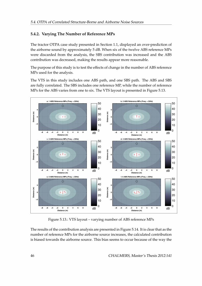
5.4. OTPA of Correlated Structure-Borne and Airborne Noise Sources
5.4.2. Varying The Number of Reference MPs
The tractor OTPA case study presented in Section 1.1, displayed an over-prediction ofthe airborne sound by approximately 5 dB. When six of the twelve ABS reference MPswere discarded from the analysis, the SBS contribution was increased and the ABScontribution was decreased, making the results appear more reasonable.
The purpose of this study is to test the effects of change in the number of ABS referenceMPs used for the analysis.
The VTS in this study includes one ABS path, and one SBS path. The ABS and SBSare fully correlated. The SBS includes one reference MP, while the number of referenceMPs for the ABS varies from one to six. The VTS layout is presented in Figure 5.13.
Distance (m)
Dis
tan
ce (
m)
a. 1 ABS Reference MPs (Freq. = 25Hz)
!8 !6 !4 !2 0 2 4 6 8
!5
0
5
dB0
10
20
30
40
50
Distance (m)
Dis
tan
ce (
m)
b. 2 ABS Reference MPs (Freq. = 25Hz)
!8 !6 !4 !2 0 2 4 6 8
!5
0
5
dB0
10
20
30
40
50
Distance (m)
Dis
tan
ce (
m)
c. 3 ABS Reference MPs (Freq. = 25Hz)
!8 !6 !4 !2 0 2 4 6 8
!5
0
5
dB0
10
20
30
40
50
Distance (m)
Dis
tan
ce (
m)
d. 4 ABS Reference MPs (Freq. = 25Hz)
!8 !6 !4 !2 0 2 4 6 8
!5
0
5
dB0
10
20
30
40
50
Distance (m)
Dis
tan
ce (
m)
e. 5 ABS Reference MPs (Freq. = 25Hz)
!8 !6 !4 !2 0 2 4 6 8
!5
0
5
dB0
10
20
30
40
50
Distance (m)
Dis
tan
ce (
m)
f. 6 ABS Reference MPs (Freq. = 25Hz)
!8 !6 !4 !2 0 2 4 6 8
!5
0
5
dB0
10
20
30
40
50
Figure 5.13.: VTS layout – varying number of ABS reference MPs
The results of the contribution analysis are presented in Figure 5.14. It is clear that as thenumber of reference MPs for the airborne source increases, the calculated contributionis biased towards the airborne source. This bias seems to occur because of the way the
46 CHALMERS, Master’s Thesis 2012:141
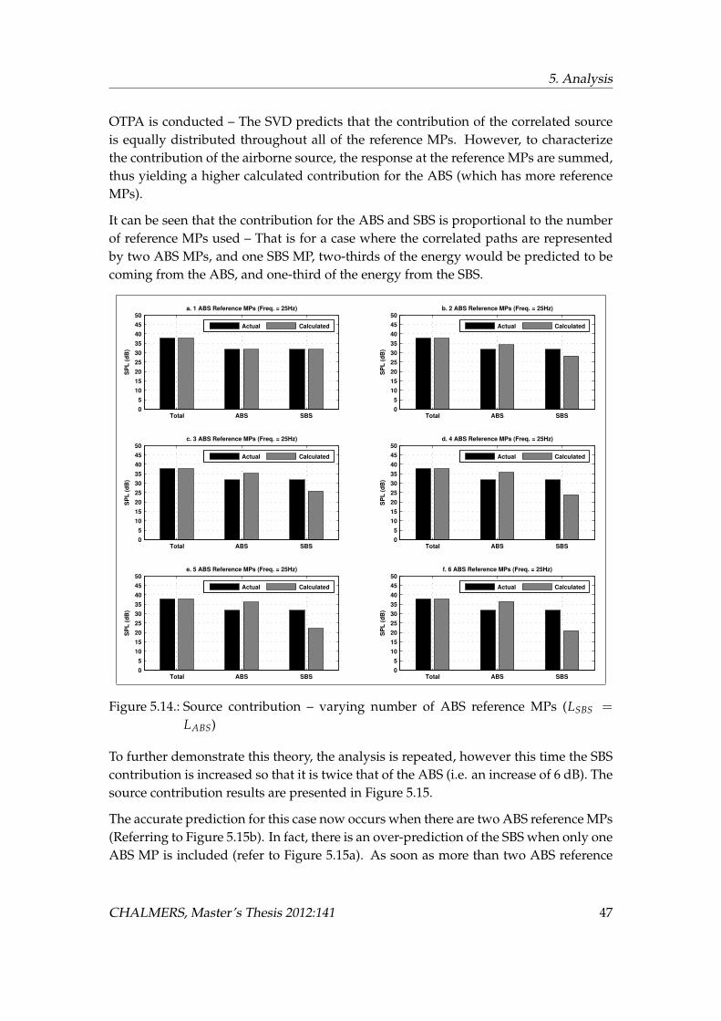
5. Analysis
OTPA is conducted – The SVD predicts that the contribution of the correlated sourceis equally distributed throughout all of the reference MPs. However, to characterizethe contribution of the airborne source, the response at the reference MPs are summed,thus yielding a higher calculated contribution for the ABS (which has more referenceMPs).
It can be seen that the contribution for the ABS and SBS is proportional to the numberof reference MPs used – That is for a case where the correlated paths are representedby two ABS MPs, and one SBS MP, two-thirds of the energy would be predicted to becoming from the ABS, and one-third of the energy from the SBS.
Total ABS SBS0
5
10
15
20
25
30
35
40
45
50
SP
L (
dB
)
a. 1 ABS Reference MPs (Freq. = 25Hz)
Actual Calculated
Total ABS SBS0
5
10
15
20
25
30
35
40
45
50
SP
L (
dB
)
b. 2 ABS Reference MPs (Freq. = 25Hz)
Actual Calculated
Total ABS SBS0
5
10
15
20
25
30
35
40
45
50
SP
L (
dB
)
c. 3 ABS Reference MPs (Freq. = 25Hz)
Actual Calculated
Total ABS SBS0
5
10
15
20
25
30
35
40
45
50
SP
L (
dB
)
d. 4 ABS Reference MPs (Freq. = 25Hz)
Actual Calculated
Total ABS SBS0
5
10
15
20
25
30
35
40
45
50
SP
L (
dB
)
e. 5 ABS Reference MPs (Freq. = 25Hz)
Actual Calculated
Total ABS SBS0
5
10
15
20
25
30
35
40
45
50
SP
L (
dB
)
f. 6 ABS Reference MPs (Freq. = 25Hz)
Actual Calculated
Figure 5.14.: Source contribution – varying number of ABS reference MPs (LSBS =LABS)
To further demonstrate this theory, the analysis is repeated, however this time the SBScontribution is increased so that it is twice that of the ABS (i.e. an increase of 6 dB). Thesource contribution results are presented in Figure 5.15.
The accurate prediction for this case now occurs when there are two ABS reference MPs(Referring to Figure 5.15b). In fact, there is an over-prediction of the SBS when only oneABS MP is included (refer to Figure 5.15a). As soon as more than two ABS reference
CHALMERS, Master’s Thesis 2012:141 47

5.4. OTPA of Correlated Structure-Borne and Airborne Noise Sources
Total ABS SBS0
5
10
15
20
25
30
35
40
45
50
SP
L (
dB
)
a. 1 ABS Reference MPs (Freq. = 25Hz)
Actual Calculated
Total ABS SBS0
5
10
15
20
25
30
35
40
45
50
SP
L (
dB
)
b. 2 ABS Reference MPs (Freq. = 25Hz)
Actual Calculated
Total ABS SBS0
5
10
15
20
25
30
35
40
45
50
SP
L (
dB
)
c. 3 ABS Reference MPs (Freq. = 25Hz)
Actual Calculated
Total ABS SBS0
5
10
15
20
25
30
35
40
45
50
SP
L (
dB
)
d. 4 ABS Reference MPs (Freq. = 25Hz)
Actual Calculated
Total ABS SBS0
5
10
15
20
25
30
35
40
45
50
SP
L (
dB
)
e. 5 ABS Reference MPs (Freq. = 25Hz)
Actual Calculated
Total ABS SBS0
5
10
15
20
25
30
35
40
45
50
SP
L (
dB
)
f. 6 ABS Reference MPs (Freq. = 25Hz)
Actual Calculated
Figure 5.15.: Source contribution – varying number of ABS reference MPs (LSBS =2LABS)
MPs are included, an over-prediction of the ABS contribution (and under-predictionsof SBS contribution) occurs again.
These results are an indication that the number of ABS reference MPs used for a sourceinfluence the results if there is a strong contribution from a correlated SBS – to avoidthis error, the ABS reference MPs for a distinct source that are measuring the sameamplitude and phase could be combined and included in the input matrix, X(jw), asone vector of data prior to conducting the SVD computations (thus the results wouldappear as shown in Figure 5.14a) . Note that the results still may not be exact, as seenin the case with a higher SBS contribution, refer to Figure 5.15a.
Further, observe that results in Figure 5.15a also agree with the results in Section 5.3.1(Figure 5.6), where it was concluded that for correlated sources, the OTPA methodyields an over-prediction of the stronger contribution, and under-prediction of theweaker contribution.
48 CHALMERS, Master’s Thesis 2012:141

5. Analysis
The results also concur with the conclusion from Section 5.4 where the ABS referenceMPs included in the analysis that was not actually measuring a strong source pickedup cross-talk from nearby sources (which is a correlated signal to the reference MP forthe other source). This, in turn, leads to a bias in the calculated source contribution.The results indicate that the more input data from invalid ABS reference MPs includedin the analysis, the greater the error in the calculated source contribution. Note thatthe total source contribution remains accurate for all the analysis cases (refer to Figure5.14), and it is only the contribution predictions of the ABS and SBS that shift.
In conclusion, it is clear that the OTPA method is sensitive to the measurement setup– the results may be biased towards sources that include more reference MPs, whetherthe reference MPs were intended for that source or not.
5.4.3. Discussion and Summary of Results
The findings derived from the VTS including an airborne source and a structure-bornesource are summarized as follows:
1. The over-prediction of the airborne source seen in the actual measurements hasbeen successfully recreated in the VTS.
2. The analyses indicate that the number of ABS reference MPs used to measure asource may bias the results of contribution analysis towards the ABS if a strongand highly correlated contribution from the SBS is also present.
3. Cross-talk from strong sources that is not properly cancelled in the analysis willlead to erroneous results. To improve the signal-to-noise ratio at the referenceMPs, and to decrease the effects of cross-talk, the reference MPs should be placedas close as possible to the sources.
4. The ABS reference MPs for a particular source that are measuring the same am-plitude and phase should be combined and included in the OTPA computation asa single data vector for each source to avoid error in the contribution predictionresults.
5. The OTPA contribution analysis results may not be completely accurate, however,if the analysis is set up correctly, the results will lead to the correct conclusions.
In the VTS, the airborne sources are small compared to the wavelength of the soundthat is being radiated to the surrounding. In this low frequency range, the size of thesource is much smaller than one-sixth wavelength (kA
lA40 = kAa << 1), and therefore
the source radiates as a simple point source. For this case, the radiation from the sourcewill be uniform regardless of the shape of the source. At a certain frequency, wherekAa > 1, the size of the source is larger than one-sixth of the wavelength, and the radia-
CHALMERS, Master’s Thesis 2012:141 49

5.4. OTPA of Correlated Structure-Borne and Airborne Noise Sources
tion from the source will no longer be uniform. In this frequency range, the source canbe seen as a combination of multiple sources – thus, the source will exhibit directivityin the radiation pattern [2].
Because of this physical characteristic, to properly measure an airborne sound source(e.g. a vehicle engine) in the high frequency range (ka > 1), several reference MPswould be required, whereas in the low frequency range (ka << 1), a single referenceMP would be sufficient.
Based on conclusion number 4 (see above), and the physics behind sound radiation inthe two frequency ranges, it’s clear that a methodology is required to be able to char-acterize the source, while not influencing any bias in the OTPA. Two possible methodscome to mind:
The first, is a simple average of all the ABS reference MPs for each particular airbornesource, and including the data as a single vector in the input matrix. However, usingthis method the phase information may be lost.
The second method involves dividing the ABS into a low frequency component anda high frequency component. This way, the filtered data from certain reference MPscan be excluded or included from the OTPA, depending on the frequency range thatthey are assigned to measure. The data could then be combined and included in theOTPA as a single input vector (or two input vectors – one for high frequency, one forlow frequency).
50 CHALMERS, Master’s Thesis 2012:141

6. Summary and Conclusions
The objective of this thesis work was to study the OTPA method and investigate thepotential causes of the over-prediction of airborne sound contribution that has occurredin some MBBMS projects. The OTPA investigation was conducted using a simplifiedvirtual test setup (VTS), consisting of two sources and one receiver, programmed usingMATLAB.
The VTS and OTPA programs were validated using a simple test setup consisting oftwo airborne sources. Further, the CTC algorithm, which uses SVD and PCA, wasvalidated by removing noise introduced to the input signals.
The analysis using the VTS commenced with a study of two airborne sources – first asfully correlated sources, then as fully uncorrelated sources. Next, a study of the effectsof including a "falsely identified source" and a correlated structure-borne sound pathin the VTS was conducted. The study also included the effects of distance between theadditional MPs (i.e. associated with the falsely identified source) and the number ofMPs for a particular source.
Subsequently, the result of the tractor OTPA case study presented in Section 1.1 wassuccessfully recreated using the VTS. By recreating the real-life problem in the VTS, itis assumed that the conclusions drawn from the VTS also apply to actual OTPA.
Several conclusions have been drawn from the OTPA study using the VTS. These con-clusions, which are relevant mainly to OTPA applied to airborne sound, are summa-rized in the following:
1. For correlated airborne sources, in order for the source contribution predictionto be accurate, the dominant sound pressure level at the reference MPs must befrom the source for which they are assigned (i.e. a good signal to noise ratio isrequired). To improve the signal-to-noise ratio, reference MPs should be placedas close as allowable to the source which they are assigned to represent.
2. Reference MPs associated with non-critical sources (i.e. falsely identified sources)will lead to incorrect source contribution results. The error is sometimes appar-ent when comparing the overall source synthesis to the actual response measure-ment, however, in some cases it may not be so clear.
51
6.1. Suggestions for Future Work
3. The number of reference MPs associated with a source has an effect on the sourcecontribution prediction results if the ABS and SBS sources/paths are highly cor-related and at similar amplitudes – the source contribution prediction results arebiased towards the source that has more reference MPs (in this case the ABS),because of the way the energy is distributed among the reference MPs of the cor-related sources/paths. To avoid this bias, the reference MPs for an individualsource/path that measures the same amplitude and phase should be combinedand included in the OTPA input matrix as a single data vector. Two methods havebeen suggested to handle this: The first, involves simply averaging the data of allthe reference MPs (however loss of phase information may occur). The secondproposed method involves assigning the reference MPs according to frequencyrange.
4. Even for an OTPA using a correct setup, the source/path contribution results maynot necessarily be completely accurate, however, the results will still lead to thecorrect practical conclusions.
6.1. Suggestions for Future Work
A few aspects of the OTPA were briefly touched upon in this thesis work that wouldbe interesting to study further. These topics are discussed in the following.
This thesis work included a study of very simple correlated and uncorrelated sourcesradiating a single tone. The SVD is only able to separate uncorrelated, or partly corre-lated data. It would be interesting to study what the upper limit of correlation betweendata sets is for the SVD and PCA algorithm to effectively separate sources/paths. Itwould also be interesting to take this study further towards a more realistic VTS byusing geometry and source signals that better represent an actual vehicle.
Further, it could be beneficial to develop an algorithm to recognize if there is significantcross-talk between the ABS reference MPs that will not be separable by using SVD(i.e. highly correlated sources/paths). This could perhaps be done, for example, byexamining the coherence, relative magnitude and phase between the data for referenceMPs. Certain reference MPs could then be excluded from the analysis computations,particularly in the low frequency range.
Once an ABS reference MP selection algorithm has successfully implemented in theVTS, it would, of course, be interesting to take the study further and use a real testsetup.
Finally, there are indications of advantages in conducting the TPA and OTPA of vehi-cle pass-by in the time domain [25]. A study of using the OTPA in the time domain,particularly for airborne sources, may yield improved results.
52 CHALMERS, Master’s Thesis 2012:141

References
[1] J.S. Bendat. Solutions for the multiple input/output problem. Journal ofSound and Vibration 44(3):311-325, 1976.
[2] L.L. Beranek. Acoustics. Acoustical Society of America, New York, 1993.
[3] H. Brick. Application of the boundary element method to combustion noiseand half-space problems. Ph.D. Thesis, Chalmers University of Technology,2009.
[4] L. Cremer et al. Structure-Borne Sound. Springer, Berlin, 2005.
[5] D. de Klerk, et al. Application of operational transfer path analysis on aclassic car. Müller-BBM VAS Special Report for DAGA 2009. Accessed fromwww.muellerbbm-vas.com on 2012.02.01.
[6] D. de Klerk. Dynamic response characterization of complex systems throughoperational identification and dynamic substructuring. Ph.D. Thesis, DelftUniversity of Technology, 2009.
[7] D. de Klerk and A. Ossipov. Operational transfer path analysis: Theory,guidelines and tire noise application. Journal of Mechanical Systems and Sig-nal Processing 24:1950-1962, 2010.
[8] G. de Sitter, et al. Operational transfer path analysis. Journal of MechanicalSystems and Signal Processing 24:416-431, 2010.
[9] P. Gajdatsy, et al. Critical assessment of operational path analysis: Effect ofcoupling between input paths. Proceedings from Acoustics ’08 Paris 5821-5826, 2008.
[10] P. Gajdatsy, et al. Critical assessment of operational path analysis: Mathemat-ical problems of transmissibility estimation. Proceedings from Acoustics ’08Paris 5463-5468, 2008.
[11] P. Gajdatsy, et al. Application of the transmissibility concept in transfer pathanalysis. Journal of Mechanical Systems and Signal Processing 24:1963-1976,2010.
53

References
[12] J.E. Jackson. A User’s Guide to Principal Components. John Wiley & SonsInc., New York, 1991.
[13] I.T. Jolliffe. Principal Component Analysis, 2nd ed. Springer-Verlag, NewYork, 2002.
[14] K. Janssens et al. Operational path analysis: A critical review. LMS Inter-national NV Technical Report, 2008. Accessed from www.lmsintl.com on2012.02.01.
[15] Müller-BBM Vibro-Acoustik Systeme. PAK v5.6. computer software. Müller-BBM VAS, 2012.
[16] K. Noumura and J. Yoshida. Method of transfer path analysis for interior ve-hicle sound by actual measurement. Japan Society of Automotive Engineers,Proceedings of The Annual Congress 55(06):7-12, 2006.
[17] P.E.F. Padhila and J.R. de França Arruda. Comparison of estimation tech-niques for vibro-acoustic transfer path analysis. Journal of Shock and Vibra-tion 13(4):459-467, 2006.
[18] J. Plunt. Finding and fixing vehicle NVH problems with transfer path analy-sis. Sound and Vibration 39:12-17, 2005.
[19] W. H. Press, et al. Numerical Recipes: The Art of Scientific Computing, 3rdEd. 65-75, Cambridge University Press, New York, 2007.
[20] A. Schuhmacher. Techniques for measuring the vibro-acoustic transfer func-tion. Sound and Vibration, March, 2010.
[21] A. Sontacchi, et al. Transfer path analysis experimental investigations andmodelling. Proceedings of the 3rd congress of the Alps Adria Acoustics As-sociation, 2007.
[22] G. Strang. Linear Algebra and its Applications. Harcourt Brace Jovanovich,Inc. Orlando, 1988.
[23] D. Tcherniak and A.P. Schuhmacher. Application of decomposition-basedtechnique in NVH source contribution analysis. Brüel & Kjær Technical Re-port for ISMA 2008. Accessed from www.bksv.com on 2012.02.01.
[24] D. Tcherniak and A.P. Schuhmacher. Application of transmissibility matrixmethod to NVH source contribution analyses. Proceedings of the IMAC-XXVII, Society for Experimental Mechanics, 2009.
[25] S. Zheng, et al. Time-domain transfer path analysis of multiple moving noisesources. Journal of Noise Control Engineering 59(5):541-548, 2011.
54 CHALMERS, Master’s Thesis 2012:141

A. MATLAB Script
A.1. MATLAB Script - Two Airborne Noise Sources
A.1.1. OTPA Script (otpa.m)
%%%%%%%%%%%%%%%%%%%%%%%%%%%%%%%%%%%%%%%%%%%%%%%%%%%%%%%%%%%%%%%%%%%%%%%%%% Operat ional Transfer Path Analysis � V i r t u a l Test Setup %% %% Mihkel Toome %% %% Descr ipt ion : %% Two sources , d i s t a n c e between sources varied %% Sources inc lude near f i e l d %% One r e f e r e n c e MP. One response MP. %% Resul t s are processed via the OTPA CTC Function . %% %% Functions a s s o c i a t e d with code ( x3 ) : %% 1 . MPs and Src/resp p o s i t i o n s defined by funct ion " d i s t .m" . %% 2 . Sources defined in INPUT . Calcs done in funct ion " source .m" . %% 3 . Countour p l o t i s setup by funct ion " contourmesh .m" . %% %% Version : 4 . 0 %% Date : 28 May 2012 %% %%%%%%%%%%%%%%%%%%%%%%%%%%%%%%%%%%%%%%%%%%%%%%%%%%%%%%%%%%%%%%%%%%%%%%%%%%t i c ;c l e a r a l l ; c l o s e a l l ; c l c ;g loba l rA rB N Nb f r_AtoB mps beta numMPs%%%%%%%%%%%%%%%%%%%%%%%%%%%%%%%%%%%%%%%%%%%%%%%%%%%%%%%%%%%%%%%%%%%%%%%%%%%% %% INPUT %% %%%%%%%%%%%%%%%%%%%%%%%%%%%%%%%%%%%%%%%%%%%%%%%%%%%%%%%%%%%%%%%%%%%%%%%%%%%%% INPUT : SrcA and SrcB proper t ies , d i s t a n c e s between Src ' s .
FreqA = 2 5 ;sizeA = 1/40; % Size ( radius ) of s p h e r i c a l SrcA r e l . to lambda A.Va = 6 0 ;NAfact = 0 . 2 ; % Amplitude of noise ( r e l a t i v e to Va )rA = 1/16; % d i s t a n c e between SrcA and r e f MPs ( r e l . to lambda A)
FreqB = 5 0 ;beta = 0* pi ; % Assign phase s h i f t f o r Source B [ radians ]sizeB = sizeA ; % Size of s p h e r i c a l SrcB r e l . to lambda A.Vb = ( FreqA/FreqB ) *Va ;
55

A.1. MATLAB Script - Two Airborne Noise Sources
NBfact = 0 . 2 ; % Amplitude of noise ( r e l a t i v e to Vb)rB = rA ; % d i s t a n c e between SrcB and r e f MPs ( r e l . to lambda A)
% vector to vary d i s t a n c e between SrcA and SrcB ( r e l . to lambda A)r_AtoB = [0 1/8 1/6 1/4 1/2 1 ] ;
numMPs = 1 ; % Define number of MPs f o r the sources
%%%%%%%%%%%%%%%%%%%%%%%%%%%%%%%%%%%%%%%%%%%%%%%%%%%%%%%%%%%%%%%%%%%%%%%%%%%% INPUT : PCA Contr ibut ion Threshold
% S e l e c t PCA methodPCA_METHOD = ' t h r e s ' ; % ' thres ' or ' cumcon ' or ' PCs ' or 'minPC '
% Input value according to s e l e c t e d PCA methodthres = 5 ; %Threshold : Minimum PCs % c o n t r i b u t i o n towards PCs score ( e . g . %5, t h r e s -
=5)cumcon = 8 5 ; % Cumulative Contr ibut ion of PCs c o n t r i b u t i n g to % of s i g n a lPCs = 2 ; % # of p r i n c i p a l components to be use in a n a l y s i sminPC = 8000 ; % Minimum magnitude of the PCs to be included
%%%%%%%%%%%%%%%%%%%%%%%%%%%%%%%%%%%%%%%%%%%%%%%%%%%%%%%%%%%%%%%%%%%%%%%%%%%% INPUT : Turn Figures on/ o f f ; p r i n t f i g u r e s on/ o f f .plotspectrum = ' o f f ' ; % P l o t spectrum f i g u r e s ' on ' / ' o f f 'plotbar = ' on ' ; % Contr ibut ion bar graph ' on/of f 'plotcontour = ' o f f ' ; % P l o t contour p l o t of SPL ' on/of f '
printfigures = ' o f f ' ; % p r i n t EPS of f i g u r e s ' on ' / ' o f f '
block = 2 ; % Which block of data i s to be p l o t t e d [1 < block <Nb]
%%%%%%%%%%%%%%%%%%%%%%%%%%%%%%%%%%%%%%%%%%%%%%%%%%%%%%%%%%%%%%%%%%%%%%%%%%%%%%%%%%%%%%%%%%%%%%%%%%%%%%%%%%%%%%%%%%%%%%%%%%%%%%%%%%%%%%%%%%%%%%%%%%%%%%% %% CALCULATIONS %% %%%%%%%%%%%%%%%%%%%%%%%%%%%%%%%%%%%%%%%%%%%%%%%%%%%%%%%%%%%%%%%%%%%%%%%%%%%%
% Function c a l c u l a t e s source s t re n gt h a t MPst i c ;[ prefa , prefb , presp , pacont , pbcont ] = source ( FreqA , FreqB , Va , Vb , NAfact , NBfact , sizeA , -
sizeB ) ;toc ;
% FREQUENCY DOMAIN% Organize r e f & resp measurements i n t o matr ices X and Y% Dimensions of X : Rows=Meas . Blocks ; Columns=MPs ( f o r "N" Freq . l i n e s and% " length ( rA ) " d i s t a n c e s between SrcA and MPs) .% X = ( Meas . Blocks , MPs, Freq . Components , Src . Dis tances )X = [ prefa prefb ] ; % f r e q domain% Y = ( Meas . Blocks , Freq . Components , Src . Dis tances )Y = presp ; % f r e q domain
%%%%%%%%%%%%%%%%%%%%%%%%%%%%%%%%%%%%%%%%%%%%%%%%%%%%%%%%%%%%%%%%%%%%%%%%%%%%% Cross Talk C a n c e l l a t i o n & Transfer Function C a l c u l a t i o n ( Frequeny Domain )
f o r ii=1: length ( r_AtoB ) % Loop f o r various SrcA�MP d i s t a n c e sf o r kk=1:N % Loop f o r N FFT frequency components
56 CHALMERS, Master’s Thesis 2012:141

A. MATLAB Script
% Singular Value Decomposition (SVD) . N. B . " S " i s the matrix of PCs .[U , S , V ] = svd ( X ( : , : , kk , ii ) , ' econ ' ) ; % use " econ " to ensure S i s a square -
Matrix .
% P r i n c i p a l Component Analysis (PCA)% COEFF � The c o e f f e c i e n t s corresponding to the PCs% PC � The P r i n c i p a l Components ( i . e . the S ingular Values )% CONT � The c o n t r i b u t i o n to the o v e r a l l s i g n a l (%)
% [COEFF, PC, CONT] = pcacov ( S ) ; % Matlab funct ion f o r PCA% Equivalent c a l c . f o r the PCA matlab funct ion abovePC = diag ( S ) ;COEFF = U *S ;CONT = diag ( S ) /sum( diag ( S ) ) * 1 0 0 ;
% Find PCs t h a t corresponsd to PCA method inputi f strcmp ( PCA_METHOD , ' t h r e s ' ) == 1
numPC = f ind ( CONT>thres , 1 , ' l a s t ' ) ;e l s e i f strcmp ( PCA_METHOD , ' cumcon ' ) ==1
numPC = f ind (sum( CONT ) >cumcon , 1 , ' l a s t ' ) ;e l s e i f strcmp ( PCA_METHOD , ' PCs ' ) ==1
numPC = PCs ;e l s e i f strcmp ( PCA_METHOD , 'minPC ' ) ==1
numPC = f ind ( PC>minPC , 1 , ' l a s t ' ) ;end
% Ca l c u l a te " invSr " � The noise reduced inverse of S .invSr = zeros ( s i z e ( S ) ) ; % A l l o c a t e zeros f o r s i z e of the invSr matrixS1 = diag ( diag ( inv ( S ( 1 : numPC , 1 : numPC ) ) ) ) ;invSr ( 1 : numPC , 1 : numPC ) = S1 ( 1 : numPC , 1 : numPC ) ;
% Ssave ( : , : , kk ) =S1 ;% Usave ( : , : , kk ) =U;% Vsave ( : , : , kk ) =V;
% Ca l c u l a te noise reduced inverse of X
X_inv ( : , : , kk , ii ) = V * invSr *U ' ; % Noise reduced inverse of X
% Transfer funct ion es t imateH ( : , kk , ii ) = X_inv ( : , : , kk , ii ) *Y ( : , kk , ii ) ;
endendtoc ; t i c ;%%%%%%%%%%%%%%%%%%%%%%%%%%%%%%%%%%%%%%%%%%%%%%%%%%%%%%%%%%%%%%%%%%%%%%%%%%%%% Ca l c u l a te Synthesized Response a t Receiver ( Freq . Domain )%%%%%%%%%%%%%%%%%%%%%%%%%%%%%%%%%%%%%%%%%%%%%%%%%%%%%%%%%%%%%%%%%%%%%%%%%%%% Re�run source : Random noise i s redef ined and a random amplitude and phase% s h i f t i s introduced to the tones ( same f o r srcA and srcB )% This s imulates a sepera te measurement f o r t r a n s f e r funct ion c a l c u l a t i o n% and s y n t h e s i s c a l c u l a t i o n .c l e a r X Y prefa prefb presp pacont pbcont[ prefa , prefb , presp , pacont , pbcont ] = source ( FreqA , FreqB , Va , Vb , NAfact , NBfact , sizeA , -
sizeB ) ;% X = ( Meas . Blocks , MPs, Freq . Components , Src . Dis tances )X = [ prefa prefb ] ; % f r e q domain% Y = ( Meas . Blocks , Freq . Components , Src . Dis tances )
CHALMERS, Master’s Thesis 2012:141 57

A.1. MATLAB Script - Two Airborne Noise Sources
Y = presp ; % f r e q domain
f o r ii=1: length ( r_AtoB )f o r jj=1:Nb
f o r kk=1:N
% Take transpose of X to rearrange v a r i a b l e s f o r YsYs ( : , jj , kk , ii ) = X ( jj , : , kk , ii ) . * H ( : , kk , ii ) ' ;
% Sum f o r t o t a l s y n t h e s i s and source c o n t r i b u t i o n s% Sum i s as i f f o r cont inuat ion of matrix m u l t i p l i c a t i o n% ( Ys=XH)Ystot ( kk , jj , ii ) = sum( Ys ( : , jj , kk , ii ) ) ;Ys_srcA ( kk , jj , ii ) = sum( Ys ( 1 : numMPs , jj , kk , ii ) ) ;Ys_srcB ( kk , jj , ii ) = sum( Ys ( numMPs + 1 : 2 * numMPs , jj , kk , ii ) ) ;
endend
end[ prespmeshA , prespmeshB , x , y ] = contourmesh ( FreqA , FreqB ) ;toc ;
A.1.2. Function to Define The Virtual Test Setup Layout (dist.m)
% Define source & r e c e i v e r ( Reference and Response ) l o c a t i o n s as% coordinates ( x , y ) . Dis tances are mul t ip les of wavelength ( lambda=d ) .% $$$$$ SrcA to SrcB d i s t a n c e i s varied $$$$% r_AtoB � Distance betwen SrcA and SrcB% r_AA � Distance between SrcA and SrcA r e f MPs% r_BB � Distance between SrcB and SrcB r e f MPs% r_AB � Distance between SrcA and SrcB r e f MPs% r_BA � Distance between SrcB and SrcA r e f MPs% mps � Matrix of a l l Src ' s , resp , and MPs ( i . e . f o r a p l o t )% a � Radius of SrcA (1/40* lamda_SrcA )% b � Radius of SrcB (1/40* lamda_SrcA )% c � Speed of sound in a i r (340m/s )
funct ion [ r_A , r_B , r_AA , r_BB , r_AB , r_BA ] = dist ( FreqA , FreqB )g loba l rA rB c r_AtoB mps d srcA srcB numMPs
c = 3 4 0 ;lambda = c/FreqA ;d=lambda ;
% r e f B _ d i s t = rB * c/FreqA ; % Define d i s t a n c e f o r Source B r e f e r e n c e -p o s i t i o n s
coords = [�d , 0 ; d , 0 ; 0 , d ;0 ,�d ] ;
% srcA = [ 0 , 0 ] ;% refA = rA* coords ; % Ref MPs f o r SrcA
resp = [ 0 , d/ s q r t ( pi ) ] ; % Response measurement p o s i t i o n ( r e c e i v e r )
58 CHALMERS, Master’s Thesis 2012:141

A. MATLAB Script
% r_AtoB = s q r t ( ( srcA ( 1 )�srcB ( 1 ) ) ^2+( srcA ( 2 )�srcB ( 2 ) ) ^2) ; % SrcA�SrcB d i s t a n c e i s d -/16
f o r ii=1: length ( r_AtoB ) % I t e r a t i o n f o r each SrcA to SrcB d i s t a n c e
% def ine SrcB p o s i t i o n r e l a t i v e to SrcA ( c e n t r e to c e n t r e d i s t a n c e )srcB ( ii , : ) = [ d/2*r_AtoB ( ii ) , 0 ] ;srcA ( ii , : ) = [�d/2*r_AtoB ( ii ) , 0 ] ;
% Define r e f e r e n c e MP' s f o r SrcA and SrcB ( c e n t r e to c e n t r e d i s t a n c e )f o r i = 1 : numMPs
refB (i , : , ii ) = �rB * coords (i , : ) + srcB ( ii , : ) ;refA (i , : , ii ) = rA * coords (i , : ) + srcA ( ii , : ) ;
end
% Assemble src ' s and response and r e f e r e n c e p o s i t i o n s i n t o a matrixmps ( : , : , ii ) = [ srcA ( ii , : ) ; srcB ( ii , : ) ; resp ; refA ( : , : , ii ) ; refB ( : , : , ii ) ] ;
% Distance b/w sources and r e f e r e n c e MPsf o r i=1: numMPs
r_AA (i , ii ) = s q r t ( ( refA (i , 1 , ii )�srcA ( ii , 1 ) ) ^2 + ( refA (i , 2 , ii )�srcA ( ii , 2 ) ) ^2) -;
r_BB (i , ii ) = s q r t ( ( refB (i , 1 , ii )�srcB ( ii , 1 ) ) ^2 + ( refB (i , 2 , ii )�srcB ( ii , 2 ) ) ^2) -;
r_AB (i , ii ) = s q r t ( ( refB (i , 1 , ii )�srcA ( ii , 1 ) ) ^2 + ( refB (i , 2 , ii )�srcA ( ii , 2 ) ) ^2) -;
r_BA (i , ii ) = s q r t ( ( refA (i , 1 , ii )�srcB ( ii , 1 ) ) ^2 + ( refA (i , 2 , ii )�srcB ( ii , 2 ) ) ^2) -;
end
% Distance b/w sources and response MPsr_A ( : , ii ) = s q r t ( ( resp ( 1 )�srcA ( ii , 1 ) ) ^2 + ( resp ( 2 )�srcA ( ii , 2 ) ) ^2) ;r_B ( : , ii ) = s q r t ( ( resp ( 1 )�srcB ( ii , 1 ) ) ^2 + ( resp ( 2 )�srcB ( ii , 2 ) ) ^2) ;
end
end
A.1.3. Function to Define The Source Signal (source.m)
% Create source s i g n a l s f o r otpa_vto .m a n a l y s i s .% Two sources : srcA & srcB .% This vers ion c r e a t e s a s i n g l e tone plus noise f o r each source .
func t ion [ prefa , prefb , presp , pacont , pbcont ] = source ( FreqA , FreqB , Va , Vb , NAfact , NBfact -, sizeA , sizeB )
g loba l r_AtoB c a b f Nb N A B noiseA noiseB beta numMPs%%%%%%%%%%%%%%%%%%%%%%%%%%%%%%%%%%%%%%%%%%%%%%%%%%%%%%%%%%%%%%%%%%%%%%%%%%%% Compute d i s t a n c e s between src ' s and MPs . See funct ion " d i s t .m"
[ r_A , r_B , r_AA , r_BB , r_AB , r_BA ] = dist ( FreqA , FreqB ) ;
%%%%%%%%%%%%%%%%%%%%%%%%%%%%%%%%%%%%%%%%%%%%%%%%%%%%%%%%%%%%%%%%%%%%%%%%%%%
% Random a d d i t i o n a l amplitude and phase s h i f t f o r source ( srcA=srcB )
CHALMERS, Master’s Thesis 2012:141 59

A.1. MATLAB Script - Two Airborne Noise Sources
rndamp = 10* rand ( 1 ) ;rndphase = pi * rand ( 1 ) ;
rho = 1 . 2 ;a = sizeA * ( c/FreqA/2) ; % Radius of Source A s p h e r i c a l sourceb = sizeB * ( c/FreqA/2) ; % Radius of Source B s p h e r i c a l source
N = 2 0 0 ; % Number of frequency l i n e s per samplef=1:N ; % Frequency vec tor (Hz)Nb = 1 0 ; % number of measurement blocks
% Build Input S i g n a l somegaA = 2* pi * FreqA ; % Frequency ( rad/s )kA = omegaA/c ; % wavenumber ( rad/m)
omegaB = 2* pi * FreqB ; % Frequency ( rad/s )kB = omegaB/c ; % wavenumber ( rad/m)
A = ( Va+rndamp ) * ( 1 j * omegaA *rho *a^2) /(1+1j *kA ) * exp (1j *kA *a ) ; % Amplitude f o r Source A -.
B = ( Vb+rndamp ) * ( 1 j * omegaB *rho *b^2) /(1+1j *kB ) * exp (1j *kB *b ) ; % Amplitude f o r Source B -.
%%%%%%%%%%%%%%%%%%%%%%%%%%%%%%%%%%%%%%%%%%%%%%%%%%%%%%%%%%%%%%%%%%%%%%%%%%%%% " Measured " Sound Pressure a t MPs
% Sound pressure a t r e f e r e n c e MPs (FREQUENCY DOMAIN)
f o r n = 1 : Nb% Amplitude f o r noisenoiseA = NAfact *Va * rand ( s i z e ( f ) ) ;noiseB = NBfact *Vb * rand ( s i z e ( f ) ) ;omega = 2* pi . * f ;
f o r ii=1: length ( r_AtoB )f o r i = 1 : numMPs
% Define s i g n a l as noise ( rnd amplitude , rnd phase ass ign )paan ( : , i , ii ) = noiseA ./ r_AA (i , ii ) . * exp(�1j * ( omega * r_AA (i , ii ) +rand * 2 * pi ) ) -
;pbbn ( : , i , ii ) = noiseB ./ r_BB (i , ii ) . * exp(�1j * ( omega * r_BB (i , ii ) +rand * 2 * pi ) ) -
;pabn ( : , i , ii ) = noiseA ./ r_AB (i , ii ) . * exp(�1j * ( omega * r_AB (i , ii ) +rand * 2 * pi ) ) -
;pban ( : , i , ii ) = noiseB ./ r_BA (i , ii ) . * exp(�1j * ( omega * r_BA (i , ii ) +rand * 2 * pi ) ) -
;
paa ( : , i , ii ) = paan ( : , i , ii ) ;pbb ( : , i , ii ) = pbbn ( : , i , ii ) ;pab ( : , i , ii ) = pabn ( : , i , ii ) ;pba ( : , i , ii ) = pban ( : , i , ii ) ;
% Add tone at s p e c i f i e d f r e q u e n c i e s ( inc ludes noise% c o n t r i b u t i o n )paa ( FreqA , i , ii ) = paan ( FreqA , i , ii ) + A/r_AA (i , ii ) * exp(�1j * ( omegaA * r_AA ( -
i , ii ) +rndphase ) ) ;
60 CHALMERS, Master’s Thesis 2012:141

A. MATLAB Script
pbb ( FreqB , i , ii ) = pbbn ( FreqB , i , ii ) + B/r_BB (i , ii ) * exp(�1j * ( omegaB * r_BB ( -i , ii )�beta+rndphase ) ) ;
pab ( FreqA , i , ii ) = pabn ( FreqA , i , ii ) + A/r_AB (i , ii ) * exp(�1j * ( omegaA * r_AB ( -i , ii ) +rndphase ) ) ;
pba ( FreqB , i , ii ) = pban ( FreqB , i , ii ) + B/r_BA (i , ii ) * exp(�1j * ( omegaB * r_BA ( -i , ii )�beta+rndphase ) ) ;
prefa (n , i , : , ii ) = paa ( : , i , ii ) + pba ( : , i , ii ) ;prefb (n , i , : , ii ) = pbb ( : , i , ii ) + pab ( : , i , ii ) ;
end
% Actual c o n t r i b u t i o n from Source A and Source B at r e c e i v e r
pacontn (n , : , ii ) = noiseA ./ r_A ( : , ii ) . * exp(�1j * omega *r_A ( : , ii ) ) ;pbcontn (n , : , ii ) = noiseB ./ r_B ( : , ii ) . * exp(�1j * ( omega *r_B ( : , ii )�beta ) ) ;
pacont (n , : , ii ) = pacontn (n , : , ii ) ;pbcont (n , : , ii ) = pbcontn (n , : , ii ) ;
pacont (n , FreqA , ii ) = pacont (n , FreqA , ii ) + A/r_A ( : , ii ) * exp(�1j * ( omegaA *r_A ( : , -ii ) +rndphase ) ) ;
pbcont (n , FreqB , ii ) = pbcont (n , FreqB , ii ) + B/r_B ( : , ii ) * exp(�1j * ( omegaB *r_B ( : , -ii )�beta+rndphase ) ) ;
% Sound pressure a t response MP ( r e c e i v e r )presp (n , : , ii ) = pacont (n , : , ii ) + pbcont (n , : , ii ) ;
endendend
A.2. MATLAB Script - Airborne and Structure-Borne Sources
A.2.1. OTPA Script (otpa_sbs.m)
%%%%%%%%%%%%%%%%%%%%%%%%%%%%%%%%%%%%%%%%%%%%%%%%%%%%%%%%%%%%%%%%%%%%%%%%%% Operat ional Transfer Path Analysis � V i r t u a l Test Setup %% %% Mihkel Toome %% %% Descr ipt ion : %% Two sources . Measurement p o s i t i o n s a t various d i s t a n c e s from source .%% Sources inc lude near f i e l d %% Severa l r e f e r e n c e MPs . One response MP. %% Resul t s are processed via the OTPA CTC Function . %% %% Functions a s s o c i a t e d with code ( x3 ) : %% 1 . MPs and Src/resp p o s i t i o n s defined by funct ion " d i s t _ s b s .m" . %% 2 . Sources defined in INPUT . Calcs done in funct ion " source_sbs .m" . %% 3 . Countour p l o t i s setup by funct ion " contourmesh .m" . %% %% Version : 4 . 0 %% Date : 23 Apri l 2012 %
CHALMERS, Master’s Thesis 2012:141 61

A.2. MATLAB Script - Airborne and Structure-Borne Sources
% %%%%%%%%%%%%%%%%%%%%%%%%%%%%%%%%%%%%%%%%%%%%%%%%%%%%%%%%%%%%%%%%%%%%%%%%%%t i c ;c l e a r a l l ; c l o s e a l l ; c l c ;g loba l rA rB N Nb mps beta%%%%%%%%%%%%%%%%%%%%%%%%%%%%%%%%%%%%%%%%%%%%%%%%%%%%%%%%%%%%%%%%%%%%%%%%%%%% %% INPUT %% %%%%%%%%%%%%%%%%%%%%%%%%%%%%%%%%%%%%%%%%%%%%%%%%%%%%%%%%%%%%%%%%%%%%%%%%%%%%% INPUT : SrcA and SrcB proper t ies , d i s t a n c e s between Src ' s .
FreqA = 2 5 ;sizeA = 1/40; % Size ( radius ) of s p h e r i c a l SrcA r e l . to lambda A.Va = 6 0 ;NAfact = 0 * 0 . 0 1 ; % Amplitude of noise ( r e l a t i v e to Va )rA = 1/16; % d i s t a n c e between SrcA and r e f MPs ( r e l . to lambda A)
FreqB = 2 5 ;beta = 0 ; % Assign phase s h i f t f o r Source B [ radians ]sizeB = sizeA ; % Size of s p h e r i c a l SrcB r e l . to lambda A.Vb = 0 ;NBfact = 0 ; % Amplitude of noise ( r e l a t i v e to Va )
rB = [1/16 1/10 1/8 1/6 1/4 1 / 2 ] ; % d i s t a n c e between SrcB and r e f MPs ( r e l . to -lambda A)
numA = 4 ; % Number of r e f e r e n c e MPs f o r Source A (max . 4 )numB = 4 ; % Number of a d d i t i o n a l r e f e r e n c e MPs f o r Source A (max . 4 )
Asbs = 1 ; % Amplitude of s t r u c t u r e�borne sound source ( r e l to SrcA r e f MP SPL )
%%%%%%%%%%%%%%%%%%%%%%%%%%%%%%%%%%%%%%%%%%%%%%%%%%%%%%%%%%%%%%%%%%%%%%%%%%%% INPUT : PCA Contr ibut ion Threshold
% S e l e c t PCA methodPCA_METHOD = ' t h r e s ' ; % ' thres ' or ' cumcon ' or ' PCs ' or 'minPC '
% Input value according to s e l e c t e d PCA methodthres = 5 ; %Threshold : Minimum PCs % c o n t r i b u t i o n towards PCs score ( e . g . %5, t h r e s -
=5)cumcon = 8 5 ; % Cumulative Contr ibut ion of PCs c o n t r i b u t i n g to % of s i g n a lPCs = 2 ; % # of p r i n c i p a l components to be use in a n a l y s i sminPC = 1 0 0 ; % Minimum magnitude of the PCs to be included
%%%%%%%%%%%%%%%%%%%%%%%%%%%%%%%%%%%%%%%%%%%%%%%%%%%%%%%%%%%%%%%%%%%%%%%%%%%% INPUT : Turn Figures on/ o f f ; p r i n t f i g u r e s on/ o f f .plotbar = ' on ' ; % Contr ibut ion bar graph ' on/of f 'plotcontour = ' on ' ; % P l o t contour p l o t of SPL ' on/of f '
printfigures = ' o f f ' ; % p r i n t EPS of f i g u r e s ' on ' / ' o f f '
block = 2 ; % Which block of data i s to be p l o t t e d [1 < block <Nb]
%%%%%%%%%%%%%%%%%%%%%%%%%%%%%%%%%%%%%%%%%%%%%%%%%%%%%%%%%%%%%%%%%%%%%%%%%%%%%%%%%%%%%%%%%%%%%%%%%%%%%%%%%%%%%%%%%%%%%%%%%%%%%%%%%%%%%%%%%%%%%%%%%%%%%%% %% CALCULATIONS %
62 CHALMERS, Master’s Thesis 2012:141

A. MATLAB Script
% %%%%%%%%%%%%%%%%%%%%%%%%%%%%%%%%%%%%%%%%%%%%%%%%%%%%%%%%%%%%%%%%%%%%%%%%%%%%
% Function c a l c u l a t e s source s t re n gt h a t MPst i c ;[ prefa , prefb , presp , pacont , sbs ] = source_sbs ( FreqA , FreqB , Va , Vb , NAfact , NBfact , sizeA , -
sizeB , Asbs ) ;toc ;
% FREQUENCY DOMAIN% Organize r e f & resp measurements i n t o matr ices X and Y% Dimensions of X : Rows=Meas . Blocks ; Columns=MPs ( f o r "N" Freq . l i n e s and% " length ( rA ) " d i s t a n c e s between SrcA and MPs) .i f numA == 0
X = [ prefb ( : , 1 : numB , : , : ) sbs ] ;e l s e i f numB == 0
X =[prefa ( : , 1 : numA , : , : ) sbs ] ;e l s e
% X = ( Meas . Blocks , MPs, Freq . Components , Src . Dis tances )X = [ prefa ( : , 1 : numA , : , : ) prefb ( : , 1 : numB , : , : ) sbs ] ; % f r e q domainend% Y = ( Meas . Blocks , Freq . Components , Src . Dis tances )Y = presp ; % f r e q domain
%%%%%%%%%%%%%%%%%%%%%%%%%%%%%%%%%%%%%%%%%%%%%%%%%%%%%%%%%%%%%%%%%%%%%%%%%%%%% Cross Talk C a n c e l l a t i o n & Transfer Function C a l c u l a t i o n ( Frequeny Domain )
f o r ii=1: length ( rB ) % Loop f o r various SrcA�MP d i s t a n c e sf o r kk=1:N % Loop f o r N FFT frequency components
% Singular Value Decomposition (SVD) . N. B . " S " i s the matrix of PCs .[U , S , V ] = svd ( X ( : , : , kk , ii ) , ' econ ' ) ; % use " econ " to ensure S i s a square -
Matrix .
% P r i n c i p a l Component Analysis (PCA)% COEFF � The c o e f f e c i e n t s corresponding to the PCs% PC � The P r i n c i p a l Components ( i . e . the S ingular Values )% CONT � The c o n t r i b u t i o n to the o v e r a l l s i g n a l (%)
% [COEFF, PC, CONT] = pcacov ( S ) ; % Matlab funct ion f o r PCA% Equivalent c a l c . f o r the PCA matlab funct ion abovePC = diag ( S ) ;COEFF = U *S ;CONT = diag ( S ) /sum( diag ( S ) ) * 1 0 0 ;Ssave ( : , : , kk ) =S ;% Find PCs t h a t corresponsd to PCA method inputi f strcmp ( PCA_METHOD , ' t h r e s ' ) == 1
numPC = f ind ( CONT>thres , 1 , ' l a s t ' ) ;e l s e i f strcmp ( PCA_METHOD , ' cumcon ' ) ==1
numPC = f ind (sum( CONT ) >cumcon , 1 , ' l a s t ' ) ;e l s e i f strcmp ( PCA_METHOD , ' PCs ' ) ==1
numPC = PCs ;e l s e i f strcmp ( PCA_METHOD , 'minPC ' ) ==1
numPC = f ind ( PC>minPC , 1 , ' l a s t ' ) ;end
CHALMERS, Master’s Thesis 2012:141 63

A.2. MATLAB Script - Airborne and Structure-Borne Sources
% Ca l c u l a te " invSr " � The noise reduced inverse of S .invSr = zeros ( s i z e ( S ) ) ; % A l l o c a t e zeros f o r s i z e of the invSr matrixS1 = diag ( diag ( inv ( S ( 1 : numPC , 1 : numPC ) ) ) ) ;invSr ( 1 : numPC , 1 : numPC ) = S1 ( 1 : numPC , 1 : numPC ) ;
% Ca l c u l a te noise reduced inverse of X
X_inv ( : , : , kk , ii ) = V * invSr *U ' ; % Noise reduced inverse of X
% Transfer funct ion es t imateH ( : , kk , ii ) = X_inv ( : , : , kk , ii ) *Y ( : , kk , ii ) ;
endendtoc ; t i c ;%%%%%%%%%%%%%%%%%%%%%%%%%%%%%%%%%%%%%%%%%%%%%%%%%%%%%%%%%%%%%%%%%%%%%%%%%%%%% Ca l c u l a te Synthesized Response a t Receiver ( Freq . Domain )%%%%%%%%%%%%%%%%%%%%%%%%%%%%%%%%%%%%%%%%%%%%%%%%%%%%%%%%%%%%%%%%%%%%%%%%%%%% Re�run source : Random noise i s redefined , s imulate sepera te measurements% f o r t r a n s f e r funct ion c a l c u l a t i o n and s y n t h e s i s c a l c u l a t i o n .c l e a r X Y prefa prefb presp pacont pbcont[ prefa , prefb , presp , pacont , sbs ] = source_sbs ( FreqA , FreqB , Va , Vb , NAfact , NBfact , sizeA , -
sizeB , Asbs ) ;i f numA == 0
X = [ prefb ( : , 1 : numB , : , : ) sbs ] ;e l s e i f numB == 0
X =[prefa ( : , 1 : numA , : , : ) sbs ] ;e l s e
% X = ( Meas . Blocks , MPs, Freq . Components , Src . Dis tances )X = [ prefa ( : , 1 : numA , : , : ) prefb ( : , 1 : numB , : , : ) sbs ] ; % f r e q domainend% Y = ( Meas . Blocks , Freq . Components , Src . Dis tances )Y = presp ; % f r e q domain
f o r ii=1: length ( rB )f o r jj=1:Nb
f o r kk=1:N
% Take transpose of X to rearrange v a r i a b l e s f o r YsYs ( : , jj , kk , ii ) = X ( jj , : , kk , ii ) . * H ( : , kk , ii ) ' ;
% Sum f o r t o t a l s y n t h e s i s and source c o n t r i b u t i o n s% Sum i s as i f f o r cont inuat ion of matrix m u l t i p l i c a t i o n% ( Ys=XH)
i f numA == 0Ystot ( kk , jj , ii ) = sum( Ys ( : , jj , kk , ii ) ) ;Ys_srcA ( kk , jj , ii ) = sum( Ys ( 1 : numB , jj , kk , ii ) ) ;Ys_abs ( kk , jj , ii ) = Ys_srcA ( kk , jj , ii ) ;Ys_sbs ( kk , jj , ii ) = Ys ( ( 1 + numB ) ,jj , kk , ii ) ;
e l s e i f numB == 0Ystot ( kk , jj , ii ) = sum( Ys ( : , jj , kk , ii ) ) ;Ys_srcA ( kk , jj , ii ) = sum( Ys ( 1 : numA , jj , kk , ii ) ) ;Ys_abs ( kk , jj , ii ) = Ys_srcA ( kk , jj , ii ) ;Ys_sbs ( kk , jj , ii ) = Ys ( ( 1 + numA ) ,jj , kk , ii ) ;
e l s e
64 CHALMERS, Master’s Thesis 2012:141

A. MATLAB Script
Ystot ( kk , jj , ii ) = sum ( ( Ys ( : , jj , kk , ii ) ) ) ;Ys_srcA ( kk , jj , ii ) = sum ( ( Ys ( 1 : numA+numB , jj , kk , ii ) ) ) ;Ys_abs ( kk , jj , ii ) = Ys_srcA ( kk , jj , ii ) ;Ys_sbs ( kk , jj , ii ) = Ys ( ( numA+numB+1) ,jj , kk , ii ) ;
endend
endend[ prespmeshA , prespmeshB , x , y ] = contourmesh ( FreqA , FreqB ) ;toc ;
A.2.2. Function to Define The Virtual Test Setup Layout (dist_sbs.m)
% Define source & r e c e i v e r ( Reference and Response ) l o c a t i o n s as% coordinates ( x , y ) . Dis tances are mul t ip les of wavelength ( lambda=d ) .% $$$$$ SrcB MPs d i s t a n c e i s varied $$$$% r_AtoB � Distance betwen SrcA and SrcB% r_AA � Distance between SrcA and SrcA r e f MPs% r_BB � Distance between SrcB and SrcB r e f MPs% r_AB � Distance between SrcA and SrcB r e f MPs% r_BA � Distance between SrcB and SrcA r e f MPs% mps � Matrix of a l l Src ' s , resp , and MPs ( i . e . f o r a p l o t )% a � Radius of SrcA (1/40* lamda_SrcA )% b � Radius of SrcB (1/40* lamda_SrcA )% c � Speed of sound in a i r (340m/s )
funct ion [ r_A , r_B , r_AA , r_BB , r_AB , r_BA ] = dist_sbs ( FreqA , FreqB )g loba l rA rB c mps d srcA srcB
c = 3 4 0 ;lambda = c/FreqA ;d=lambda ;
% r e f B _ d i s t = rB * c/FreqA ; % Define d i s t a n c e f o r Source B r e f e r e n c e -p o s i t i o n s
coords = [d , 0 ; 0 , d ; �d , 0 ; 0 , �d ] ;
% srcA = [ 0 , 0 ] ;% refA = rA* coords ; % Ref MPs f o r SrcA
resp = [ 0 , d/ s q r t ( pi ) ] ; % Response measurement p o s i t i o n ( r e c e i v e r )
% r_AtoB = s q r t ( ( srcA ( 1 )�srcB ( 1 ) ) ^2+( srcA ( 2 )�srcB ( 2 ) ) ^2) ; % SrcA�SrcB d i s t a n c e i s d -/16
f o r ii=1: length ( rB ) % I t e r a t i o n f o r each SrcA to SrcB d i s t a n c e
% def ine SrcB p o s i t i o n r e l a t i v e to SrcA ( c e n t r e to c e n t r e d i s t a n c e )srcB ( ii , : ) = [ 0 , 0 ] ;srcA ( ii , : ) = [ 0 , 0 ] ;
% Define r e f e r e n c e MP' s f o r SrcA and SrcB ( c e n t r e to c e n t r e d i s t a n c e )
CHALMERS, Master’s Thesis 2012:141 65
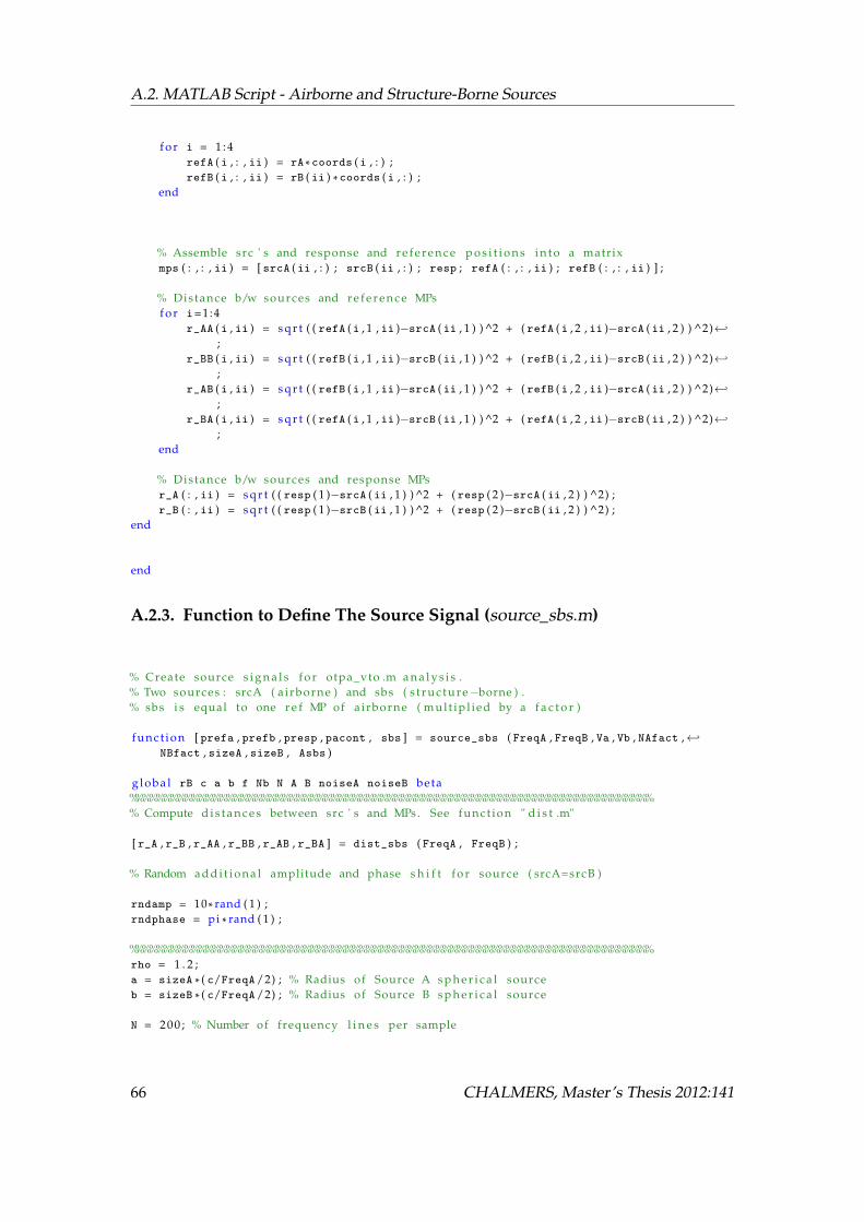
A.2. MATLAB Script - Airborne and Structure-Borne Sources
f o r i = 1 : 4refA (i , : , ii ) = rA * coords (i , : ) ;refB (i , : , ii ) = rB ( ii ) * coords (i , : ) ;
end
% Assemble src ' s and response and r e f e r e n c e p o s i t i o n s i n t o a matrixmps ( : , : , ii ) = [ srcA ( ii , : ) ; srcB ( ii , : ) ; resp ; refA ( : , : , ii ) ; refB ( : , : , ii ) ] ;
% Distance b/w sources and r e f e r e n c e MPsf o r i=1:4
r_AA (i , ii ) = s q r t ( ( refA (i , 1 , ii )�srcA ( ii , 1 ) ) ^2 + ( refA (i , 2 , ii )�srcA ( ii , 2 ) ) ^2) -;
r_BB (i , ii ) = s q r t ( ( refB (i , 1 , ii )�srcB ( ii , 1 ) ) ^2 + ( refB (i , 2 , ii )�srcB ( ii , 2 ) ) ^2) -;
r_AB (i , ii ) = s q r t ( ( refB (i , 1 , ii )�srcA ( ii , 1 ) ) ^2 + ( refB (i , 2 , ii )�srcA ( ii , 2 ) ) ^2) -;
r_BA (i , ii ) = s q r t ( ( refA (i , 1 , ii )�srcB ( ii , 1 ) ) ^2 + ( refA (i , 2 , ii )�srcB ( ii , 2 ) ) ^2) -;
end
% Distance b/w sources and response MPsr_A ( : , ii ) = s q r t ( ( resp ( 1 )�srcA ( ii , 1 ) ) ^2 + ( resp ( 2 )�srcA ( ii , 2 ) ) ^2) ;r_B ( : , ii ) = s q r t ( ( resp ( 1 )�srcB ( ii , 1 ) ) ^2 + ( resp ( 2 )�srcB ( ii , 2 ) ) ^2) ;
end
end
A.2.3. Function to Define The Source Signal (source_sbs.m)
% Create source s i g n a l s f o r otpa_vto .m a n a l y s i s .% Two sources : srcA ( a i rborne ) and sbs ( s t r u c t u r e�borne ) .% sbs i s equal to one r e f MP of a irborne ( mul t ip l ied by a f a c t o r )
funct ion [ prefa , prefb , presp , pacont , sbs ] = source_sbs ( FreqA , FreqB , Va , Vb , NAfact , -NBfact , sizeA , sizeB , Asbs )
g loba l rB c a b f Nb N A B noiseA noiseB beta%%%%%%%%%%%%%%%%%%%%%%%%%%%%%%%%%%%%%%%%%%%%%%%%%%%%%%%%%%%%%%%%%%%%%%%%%%%% Compute d i s t a n c e s between src ' s and MPs . See funct ion " d i s t .m"
[ r_A , r_B , r_AA , r_BB , r_AB , r_BA ] = dist_sbs ( FreqA , FreqB ) ;
% Random a d d i t i o n a l amplitude and phase s h i f t f o r source ( srcA=srcB )
rndamp = 10* rand ( 1 ) ;rndphase = pi * rand ( 1 ) ;
%%%%%%%%%%%%%%%%%%%%%%%%%%%%%%%%%%%%%%%%%%%%%%%%%%%%%%%%%%%%%%%%%%%%%%%%%%%rho = 1 . 2 ;a = sizeA * ( c/FreqA/2) ; % Radius of Source A s p h e r i c a l sourceb = sizeB * ( c/FreqA/2) ; % Radius of Source B s p h e r i c a l source
N = 2 0 0 ; % Number of frequency l i n e s per sample
66 CHALMERS, Master’s Thesis 2012:141
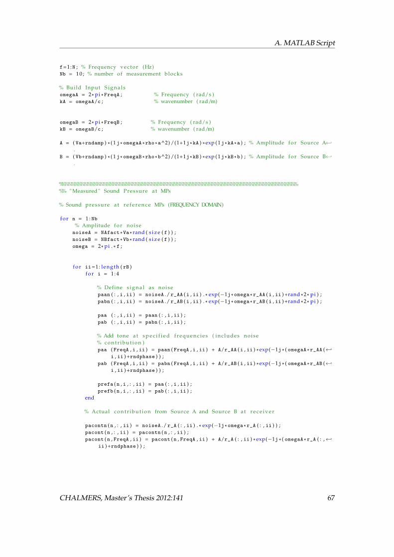
A. MATLAB Script
f=1:N ; % Frequency vec tor (Hz)Nb = 1 0 ; % number of measurement blocks
% Build Input S i g n a l somegaA = 2* pi * FreqA ; % Frequency ( rad/s )kA = omegaA/c ; % wavenumber ( rad/m)
omegaB = 2* pi * FreqB ; % Frequency ( rad/s )kB = omegaB/c ; % wavenumber ( rad/m)
A = ( Va+rndamp ) * ( 1 j * omegaA *rho *a^2) /(1+1j *kA ) * exp (1j *kA *a ) ; % Amplitude f o r Source A -.
B = ( Vb+rndamp ) * ( 1 j * omegaB *rho *b^2) /(1+1j *kB ) * exp (1j *kB *b ) ; % Amplitude f o r Source B -.
%%%%%%%%%%%%%%%%%%%%%%%%%%%%%%%%%%%%%%%%%%%%%%%%%%%%%%%%%%%%%%%%%%%%%%%%%%%%% " Measured " Sound Pressure a t MPs
% Sound pressure a t r e f e r e n c e MPs (FREQUENCY DOMAIN)
f o r n = 1 : Nb% Amplitude f o r noisenoiseA = NAfact *Va * rand ( s i z e ( f ) ) ;noiseB = NBfact *Vb * rand ( s i z e ( f ) ) ;omega = 2* pi . * f ;
f o r ii=1: length ( rB )f o r i = 1 : 4
% Define s i g n a l as noisepaan ( : , i , ii ) = noiseA ./ r_AA (i , ii ) . * exp(�1j * omega * r_AA (i , ii ) +rand * 2 * pi ) ;pabn ( : , i , ii ) = noiseA ./ r_AB (i , ii ) . * exp(�1j * omega * r_AB (i , ii ) +rand * 2 * pi ) ;
paa ( : , i , ii ) = paan ( : , i , ii ) ;pab ( : , i , ii ) = pabn ( : , i , ii ) ;
% Add tone at s p e c i f i e d f r e q u e n c i e s ( inc ludes noise% c o n t r i b u t i o n )paa ( FreqA , i , ii ) = paan ( FreqA , i , ii ) + A/r_AA (i , ii ) * exp(�1j * ( omegaA * r_AA ( -
i , ii ) +rndphase ) ) ;pab ( FreqA , i , ii ) = pabn ( FreqA , i , ii ) + A/r_AB (i , ii ) * exp(�1j * ( omegaA * r_AB ( -
i , ii ) +rndphase ) ) ;
prefa (n , i , : , ii ) = paa ( : , i , ii ) ;prefb (n , i , : , ii ) = pab ( : , i , ii ) ;
end
% Actual c o n t r i b u t i o n from Source A and Source B at r e c e i v e r
pacontn (n , : , ii ) = noiseA ./ r_A ( : , ii ) . * exp(�1j * omega *r_A ( : , ii ) ) ;pacont (n , : , ii ) = pacontn (n , : , ii ) ;pacont (n , FreqA , ii ) = pacont (n , FreqA , ii ) + A/r_A ( : , ii ) * exp(�1j * ( omegaA *r_A ( : , -
ii ) +rndphase ) ) ;
CHALMERS, Master’s Thesis 2012:141 67
A.3. Function to Plot Sound Field (contourmesh.m)
% Simulate Structure�Borne sound c o n t r i b u t i o n
sbs (n , 1 , : , ii ) = Asbs * prefa (n , 1 , : , ii ) ;
% Sound pressure a t response MP ( r e c e i v e r )presp (n , : , ii ) = pacont (n , : , ii ) + Asbs * pacont (n , : , ii ) ;
endendend
A.3. Function to Plot Sound Field (contourmesh.m)
% Function to c r e a t e data f o r contour p l o t s of the SPL over% the V i r t u a l Test Setup area . Two p l o t s a t FreqA and FreqB .
funct ion [ prespmeshA , prespmeshB , x , y ] = contourmesh ( FreqA , FreqB )g loba l A B noiseA noiseB Nb d srcA srcB beta
omegaA = 2* pi * FreqA ;omegaB = 2* pi * FreqB ;
[x , y ] =meshgrid (�0.7*d : 0 . 1 : 0 . 7 * d ,�0.7*d : 0 . 1 : 0 . 7 * d ) ; % Dims chosen to make p l o t look -nice
f o r n = 1 : Nbf o r ii=1:6
rA = s q r t ( ( x�srcA ( ii , 1 ) ) .^2+(y�srcA ( ii , 2 ) ) . ^ 2 ) ;rB = s q r t ( ( x�srcB ( ii , 1 ) ) .^2+(y�srcB ( ii , 2 ) ) . ^ 2 ) ;
pan ( : , : , ii , n ) = noiseA ( FreqA ) ./ rA . * exp(�1j * omegaA . * rA ) ;pbn ( : , : , ii , n ) = noiseB ( FreqB ) ./ rB . * exp(�1j * ( omegaB . * rB�beta ) ) ;
% Redefine tone at s p e c i f i e d f r e q u e n c i e spa ( : , : , ii , n ) = A ./ rA . * exp(�1j * omegaA . * rA ) ;pb ( : , : , ii , n ) = B ./ rB . * exp(�1j * ( omegaB . * rB�beta ) ) ;
% Add t o t a l SPL
i f FreqA==FreqBprespmeshA ( : , : , ii , n ) = pa ( : , : , ii , n ) + pb ( : , : , ii , n ) ;prespmeshB ( : , : , ii , n ) = pa ( : , : , ii , n ) + pb ( : , : , ii , n ) ;
e l s eprespmeshA ( : , : , ii , n ) = pa ( : , : , ii , n ) + pbn ( : , : , ii , n ) ;prespmeshB ( : , : , ii , n ) = pb ( : , : , ii , n ) + pan ( : , : , ii , n ) ;
endend
end
end
68 CHALMERS, Master’s Thesis 2012:141

A. MATLAB Script
A.4. MATLAB Script - Airborne and Structure-Borne Sources,Varied Number of Reference MPs
A.4.1. OTPA Script (otpa_sbs_num.m)
%%%%%%%%%%%%%%%%%%%%%%%%%%%%%%%%%%%%%%%%%%%%%%%%%%%%%%%%%%%%%%%%%%%%%%%%%% Operat ional Transfer Path Analysis � V i r t u a l Test Setup %% %% Mihkel Toome %% %% Descr ipt ion : %% Two sources : ABS and SBS . %% Measurement p o s i t i o n s a t various d i s t a n c e s from source . %% Sources inc lude near f i e l d %% Severa l r e f e r e n c e MPs . One response MP. %% Resul t s are processed via the OTPA CTC Function . %% %% Functions a s s o c i a t e d with code ( x3 ) : %% 1 . MPs and Src/resp p o s i t i o n s defined by funct ion " d i s t _ s b s .m" . %% 2 . Sources defined in INPUT . Calcs done in funct ion " source_sbs .m" . %% 3 . Countour p l o t i s setup by funct ion " contourmesh .m" . %% %% %% %%%%%%%%%%%%%%%%%%%%%%%%%%%%%%%%%%%%%%%%%%%%%%%%%%%%%%%%%%%%%%%%%%%%%%%%%%t i c ;c l e a r a l l ; c l o s e a l l ; c l c ;g loba l rA N Nb mps numA%%%%%%%%%%%%%%%%%%%%%%%%%%%%%%%%%%%%%%%%%%%%%%%%%%%%%%%%%%%%%%%%%%%%%%%%%%%% %% INPUT %% %%%%%%%%%%%%%%%%%%%%%%%%%%%%%%%%%%%%%%%%%%%%%%%%%%%%%%%%%%%%%%%%%%%%%%%%%%%%% INPUT : SrcA and SrcB proper t ies , d i s t a n c e s between Src ' s .
FreqA = 2 5 ;sizeA = 1/40; % Size ( radius ) of s p h e r i c a l SrcA r e l . to lambda A.Va = 6 0 ;NAfact = 0 * 0 . 0 1 ; % Amplitude of noise ( r e l a t i v e to Va )rA = 1/16; % d i s t a n c e between SrcA and r e f MPs ( r e l . to lambda A)
numA = [1 2 3 4 5 6 ] ; % Number of r e f e r e n c e MPs f o r Source A
Asbs = 2 ; % Amplitude of s t r u c t u r e�borne sound source ( r e l to SrcA r e f MP SPL )
%%%%%%%%%%%%%%%%%%%%%%%%%%%%%%%%%%%%%%%%%%%%%%%%%%%%%%%%%%%%%%%%%%%%%%%%%%%% INPUT : PCA Contr ibut ion Threshold
% S e l e c t PCA methodPCA_METHOD = ' t h r e s ' ; % ' thres ' or ' cumcon ' or ' PCs ' or 'minPC '
% Input value according to s e l e c t e d PCA method
CHALMERS, Master’s Thesis 2012:141 69

A.4. MATLAB Script - Airborne and Structure-Borne Sources, Varied Number ofReference MPs
thres = 5 ; %Threshold : Minimum PCs % c o n t r i b u t i o n towards PCs score ( e . g . %5, t h r e s -=5)
cumcon = 8 5 ; % Cumulative Contr ibut ion of PCs c o n t r i b u t i n g to % of s i g n a lPCs = 2 ; % # of p r i n c i p a l components to be use in a n a l y s i sminPC = 1 0 0 ; % Minimum magnitude of the PCs to be included
%%%%%%%%%%%%%%%%%%%%%%%%%%%%%%%%%%%%%%%%%%%%%%%%%%%%%%%%%%%%%%%%%%%%%%%%%%%% INPUT : Turn Figures on/ o f f ; p r i n t f i g u r e s on/ o f f .plotbar = ' on ' ; % Contr ibut ion bar graph ' on/of f 'plotcontour = ' on ' ; % P l o t contour p l o t of SPL ' on/of f '
printfigures = ' o f f ' ; % p r i n t EPS of f i g u r e s ' on ' / ' o f f '
block = 2 ; % Which block of data i s to be p l o t t e d [1 < block <Nb]
%%%%%%%%%%%%%%%%%%%%%%%%%%%%%%%%%%%%%%%%%%%%%%%%%%%%%%%%%%%%%%%%%%%%%%%%%%%%%%%%%%%%%%%%%%%%%%%%%%%%%%%%%%%%%%%%%%%%%%%%%%%%%%%%%%%%%%%%%%%%%%%%%%%%%%% %% CALCULATIONS %% %%%%%%%%%%%%%%%%%%%%%%%%%%%%%%%%%%%%%%%%%%%%%%%%%%%%%%%%%%%%%%%%%%%%%%%%%%%%
%%%%%%%%%%%%%%%%%%%%%%%%%%%%%%%%%%%%%%%%%%%%%%%%%%%%%%%%%%%%%%%%%%%%%%%%%%%%% Cross Talk C a n c e l l a t i o n & Transfer Function C a l c u l a t i o n ( Frequeny Domain )
f o r ii=1: length ( numA ) % Loop f o r various SrcA�MP d i s t a n c e s
% Function c a l c u l a t e s source s t re n gt h a t MPst i c ;[ prefa , presp , pacont , sbs ] = source_sbs_num ( FreqA , Va , NAfact , sizeA , Asbs ) ;toc ;% FREQUENCY DOMAIN% Organize r e f & resp measurements i n t o matr ices X and Y% Dimensions of X : Rows=Meas . Blocks ; Columns=MPs ( f o r "N" Freq . l i n e s and% " length ( rA ) " d i s t a n c e s between SrcA and MPs) .
% X = ( Meas . Blocks , MPs, Freq . Components )X = [ prefa ( : , 1 : numA ( ii ) , : ) sbs ] ; % f r e q domain% Y = ( Meas . Blocks , Freq . Components , Src . Dis tances )Y = presp ; % f r e q domain
f o r kk=1:N % Loop f o r N FFT frequency components
% Singular Value Decomposition (SVD) . N. B . " S " i s the matrix of PCs .[U , S , V ] = svd ( X ( : , : , kk ) , ' econ ' ) ; % use " econ " to ensure S i s a square -
Matrix .
% P r i n c i p a l Component Analysis (PCA)% COEFF � The c o e f f e c i e n t s corresponding to the PCs% PC � The P r i n c i p a l Components ( i . e . the S ingular Values )% CONT � The c o n t r i b u t i o n to the o v e r a l l s i g n a l (%)
% [COEFF, PC, CONT] = pcacov ( S ) ; % Matlab funct ion f o r PCA% Equivalent c a l c . f o r the PCA matlab funct ion abovePC = diag ( S ) ;COEFF = U *S ;
70 CHALMERS, Master’s Thesis 2012:141

A. MATLAB Script
CONT = diag ( S ) /sum( diag ( S ) ) * 1 0 0 ;% Ssave ( : , : , kk ) =S ;
% Find PCs t h a t corresponsd to PCA method inputi f strcmp ( PCA_METHOD , ' t h r e s ' ) == 1
numPC = f ind ( CONT>thres , 1 , ' l a s t ' ) ;e l s e i f strcmp ( PCA_METHOD , ' cumcon ' ) ==1
numPC = f ind (sum( CONT ) >cumcon , 1 , ' l a s t ' ) ;e l s e i f strcmp ( PCA_METHOD , ' PCs ' ) ==1
numPC = PCs ;e l s e i f strcmp ( PCA_METHOD , 'minPC ' ) ==1
numPC = f ind ( PC>minPC , 1 , ' l a s t ' ) ;end
% Ca l c u l a te " invSr " � The noise reduced inverse of S .invSr = zeros ( s i z e ( S ) ) ; % A l l o c a t e zeros f o r s i z e of the invSr matrixS1 = diag ( diag ( inv ( S ( 1 : numPC , 1 : numPC ) ) ) ) ;invSr ( 1 : numPC , 1 : numPC ) = S1 ( 1 : numPC , 1 : numPC ) ;
% Ca l c u l a te noise reduced inverse of X
X_inv = V * invSr *U ' ; % Noise reduced inverse of X
% Transfer funct ion es t imateH ( : , kk ) = X_inv *Y ( : , kk ) ;
end
toc ; t i c ;%%%%%%%%%%%%%%%%%%%%%%%%%%%%%%%%%%%%%%%%%%%%%%%%%%%%%%%%%%%%%%%%%%%%%%%%%%%%% Ca l c u l a te Synthesized Response a t Receiver ( Freq . Domain )%%%%%%%%%%%%%%%%%%%%%%%%%%%%%%%%%%%%%%%%%%%%%%%%%%%%%%%%%%%%%%%%%%%%%%%%%%%% Re�run source : Random noise i s redefined , s imulate sepera te measurements% f o r t r a n s f e r funct ion c a l c u l a t i o n and s y n t h e s i s c a l c u l a t i o n .c l e a r X Y prefa presp pacont sbs[ prefa , presp , pacont , sbs ] = source_sbs_num ( FreqA , Va , NAfact , sizeA , Asbs ) ;
% % X = ( Meas . Blocks , MPs, Freq . Components , Src . Dis tances )X = [ prefa ( : , 1 : numA ( ii ) , : ) sbs ] ; % f r e q domain% Y = ( Meas . Blocks , Freq . Components , Src . Dis tances )Y = presp ; % f r e q domain
f o r jj=1:Nbf o r kk=1:N
% Take transpose of X to rearrange v a r i a b l e s f o r YsYs ( : , jj , kk ) = X ( jj , : , kk ) ' . * H ( : , kk ) ;
% Sum f o r t o t a l s y n t h e s i s and source c o n t r i b u t i o n s% Sum i s as i f f o r cont inuat ion of matrix m u l t i p l i c a t i o n% ( Ys=XH)
Ystot ( kk , jj , ii ) = sum ( ( Ys ( : , jj , kk ) ) ) ;Ys_srcA ( kk , jj , ii ) = sum( Ys ( 1 : numA ( ii ) ,jj , kk ) ) ;Ys_abs ( kk , jj , ii ) = Ys_srcA ( kk , jj , ii ) ;Ys_sbs ( kk , jj , ii ) = Ys ( end , jj , kk ) ;
end
CHALMERS, Master’s Thesis 2012:141 71

A.4. MATLAB Script - Airborne and Structure-Borne Sources, Varied Number ofReference MPs
end
c l e a r H X Ys
end[ prespmeshA , x , y ] = contourmesh_num ( FreqA ) ;
toc ;
A.4.2. Function to Define The Virtual Test Setup Layout (dist_sbs_num.m)
% Define source & r e c e i v e r ( Reference and Response ) l o c a t i o n s as% coordinates ( x , y ) . Dis tances are mul t ip les of wavelength ( lambda=d ) .% $$$$$ SrcB MPs d i s t a n c e i s varied $$$$% r_AtoB � Distance betwen SrcA and SrcB% r_AA � Distance between SrcA and SrcA r e f MPs% r_BB � Distance between SrcB and SrcB r e f MPs% r_AB � Distance between SrcA and SrcB r e f MPs% r_BA � Distance between SrcB and SrcA r e f MPs% mps � Matrix of a l l Src ' s , resp , and MPs ( i . e . f o r a p l o t )% a � Radius of SrcA (1/40* lamda_SrcA )% b � Radius of SrcB (1/40* lamda_SrcA )% c � Speed of sound in a i r (340m/s )
funct ion [ r_A , r_AA ] = dist_sbs_num ( FreqA )g loba l rA c mps d srcA numA
c = 3 4 0 ;lambda = c/FreqA ;d=lambda ;
% r e f B _ d i s t = rB * c/FreqA ; % Define d i s t a n c e f o r Source B r e f e r e n c e -p o s i t i o n s
coords = [d , 0 ; 0 , d ; �d , 0 ; 0 , �d ; d/ s q r t ( 2 ) , d/ s q r t ( 2 ) ; �d/ s q r t ( 2 ) , �d/ s q r t ( 2 ) ] ;
srcA = [ 0 , 0 ] ;% refA = rA* coords ; % Ref MPs f o r SrcA
resp = [ 0 , d/ s q r t ( pi ) ] ; % Response measurement p o s i t i o n ( r e c e i v e r )
% Define r e f e r e n c e MP' s f o r SrcA and SrcB ( c e n t r e to c e n t r e d i s t a n c e )f o r i = 1 : length ( numA )
refA (i , : ) = rA * coords (i , : ) ;
end
% Assemble src ' s and response and r e f e r e n c e p o s i t i o n s i n t o a matrixmps = [ srcA ; resp ; refA ] ;
% Distance b/w sources and r e f e r e n c e MPsf o r i=1: length ( numA )
r_AA ( i ) = s q r t ( ( refA (i , 1 )�srcA ( 1 ) ) ^2 + ( refA (i , 2 )�srcA ( 2 ) ) ^2) ;end
% Distance b/w sources and response MPs
72 CHALMERS, Master’s Thesis 2012:141

A. MATLAB Script
r_A = s q r t ( ( resp ( 1 )�srcA ( 1 ) ) ^2 + ( resp ( 2 )�srcA ( 2 ) ) ^2) ;
end
A.4.3. Function to Define The Source Signal (source_sbs_num.m)
% Create source s i g n a l s f o r otpa_vto .m a n a l y s i s .% Two sources : srcA ( a i rborne ) and sbs ( s t r u c t u r e�borne ) .% sbs i s equal to one r e f MP of a irborne ( mul t ip l ied by a f a c t o r )
funct ion [ prefa , presp , pacont , sbs ] = source_sbs_num ( FreqA , Va , NAfact , sizeA , Asbs )
g loba l c a f Nb N A noiseA numA%%%%%%%%%%%%%%%%%%%%%%%%%%%%%%%%%%%%%%%%%%%%%%%%%%%%%%%%%%%%%%%%%%%%%%%%%%%% Compute d i s t a n c e s between src ' s and MPs . See funct ion " d i s t .m"
[ r_A , r_AA ] = dist_sbs_num ( FreqA ) ;
%%%%%%%%%%%%%%%%%%%%%%%%%%%%%%%%%%%%%%%%%%%%%%%%%%%%%%%%%%%%%%%%%%%%%%%%%%%
% Random a d d i t i o n a l amplitude and phase s h i f t f o r source ( srcA=srcB )rndamp = 10* rand ( 1 ) ;rndphase = pi * rand ( 1 ) ;
rho = 1 . 2 ;a = sizeA * ( c/FreqA/2) ; % Radius of Source A s p h e r i c a l source
N = 2 0 0 ; % Number of frequency l i n e s per samplef=1:N ; % Frequency vec tor (Hz)Nb = 1 0 ; % number of measurement blocks
% Build Input S i g n a l somegaA = 2* pi * FreqA ; % Frequency ( rad/s )kA = omegaA/c ; % wavenumber ( rad/m)
A = ( Va+rndamp ) * ( 1 j * omegaA *rho *a^2) /(1+1j *kA ) * exp (1j *kA *a ) ; % Amplitude f o r Source A -.
%%%%%%%%%%%%%%%%%%%%%%%%%%%%%%%%%%%%%%%%%%%%%%%%%%%%%%%%%%%%%%%%%%%%%%%%%%%%% " Measured " Sound Pressure a t MPs
% Sound pressure a t r e f e r e n c e MPs (FREQUENCY DOMAIN)
f o r n = 1 : Nb% Amplitude f o r noisenoiseA = NAfact *Va * rand ( s i z e ( f ) ) ;omega = 2* pi . * f ;
f o r i = 1 : length ( numA )
% Define s i g n a l as noisepaan ( : , i ) = noiseA ./ r_AA ( i ) . * exp(�1j * omega * r_AA ( i ) +rand * 2 * pi ) ;
CHALMERS, Master’s Thesis 2012:141 73

A.4. MATLAB Script - Airborne and Structure-Borne Sources, Varied Number ofReference MPs
paa ( : , i ) = paan ( : , i ) ;
% Add tone at s p e c i f i e d f r e q u e n c i e s ( inc ludes noise% c o n t r i b u t i o n )paa ( FreqA , i ) = paan ( FreqA , i ) + A/r_AA ( i ) * exp(�1j * ( omegaA * r_AA ( i ) + -
rndphase ) ) ;prefa (n , i , : ) = paa ( : , i ) ;
end
% Actual c o n t r i b u t i o n from Source A and Source B at r e c e i v e r
pacontn (n , : ) = noiseA ./ r_A ( : ) . * exp(�1j * omega *r_A ) ;pacont (n , : ) = pacontn (n , : ) ;pacont (n , FreqA ) = pacont (n , FreqA ) + A/r_A * exp(�1j * ( omegaA *r_A+rndphase ) ) ;
% Simulate Structure�Borne sound c o n t r i b u t i o n
sbs (n , 1 , : ) = Asbs * prefa (n , 1 , : ) ;
% Sound pressure a t response MP ( r e c e i v e r )presp (n , : ) = pacont (n , : ) + Asbs * pacont (n , : ) ;
endend
A.4.4. Function to Plot Sound Field (contourmesh_num.m)
% Function to c r e a t e data f o r contour p l o t s of the SPL over% the V i r t u a l Test Setup area . Two p l o t s a t FreqA and FreqB .
funct ion [ prespmeshA , x , y ] = contourmesh_num ( FreqA )g loba l A noiseA Nb d srcA
omegaA = 2* pi * FreqA ;
[x , y ] =meshgrid (�0.7*d : 0 . 0 5 : 0 . 7 * d ,�0.7*d : 0 . 0 5 : 0 . 7 * d ) ; % Dims chosen to make p l o t -look nice
f o r n = 1 : Nb
rA = s q r t ( ( x�srcA ( 1 ) ) .^2+(y�srcA ( 2 ) ) . ^ 2 ) ;pan ( : , : , n ) = noiseA ( FreqA ) ./ rA . * exp(�1j * omegaA . * rA ) ;
% Redefine tone at s p e c i f i e d f r e q u e n c i e spa ( : , : , n ) = A ./ rA . * exp(�1j * omegaA . * rA ) ;
% Add t o t a l SPL
prespmeshA ( : , : , n ) = pa ( : , : , n ) + pan ( : , : , n ) ;end
end
74 CHALMERS, Master’s Thesis 2012:141


![THE OSS EVOLUTIONARY PATH TO OPERATIONAL/BUSINESS BENEFITS · THE OSS EVOLUTIONARY PATH TO OPERATIONAL/BUSINESS ... (eTOM) to manage business processes [1], ... dimension of eTOM](https://img.pdfslide.us/doc/110x75/5ad4dedd7f8b9a5d058c7226/the-oss-evolutionary-path-to-operationalbusiness-oss-evolutionary-path-to-operationalbusiness.jpg)