See discussions, stats, and author profiles for this publication at: https://www.researchgate.net/publication/259508465

Modeling fluid-structure interaction by the Particle Finite Element Method in

OpenSees

Article  in  Computers & Structures · February 2014

DOI: 10.1016/j.compstruc.2013.11.002

CITATIONS

22READS

870

2 authors:

Some of the authors of this publication are also working on these related projects:

OpenSees Blog View project

Simulation of Tsunami and Infrastructure View project

Minjie Zhu

Oregon State University

9 PUBLICATIONS   64 CITATIONS   

SEE PROFILE

Michael H. Scott

Oregon State University

59 PUBLICATIONS   946 CITATIONS   

SEE PROFILE

All content following this page was uploaded by Minjie Zhu on 06 September 2018.

The user has requested enhancement of the downloaded file.

This article appeared in a journal published by Elsevier. The attachedcopy is furnished to the author for internal non-commercial researchand education use, including for instruction at the authors institution

and sharing with colleagues.

Other uses, including reproduction and distribution, or selling orlicensing copies, or posting to personal, institutional or third party

websites are prohibited.

In most cases authors are permitted to post their version of thearticle (e.g. in Word or Tex form) to their personal website orinstitutional repository. Authors requiring further information

regarding Elsevier’s archiving and manuscript policies areencouraged to visit:

http://www.elsevier.com/authorsrights

Author's personal copy

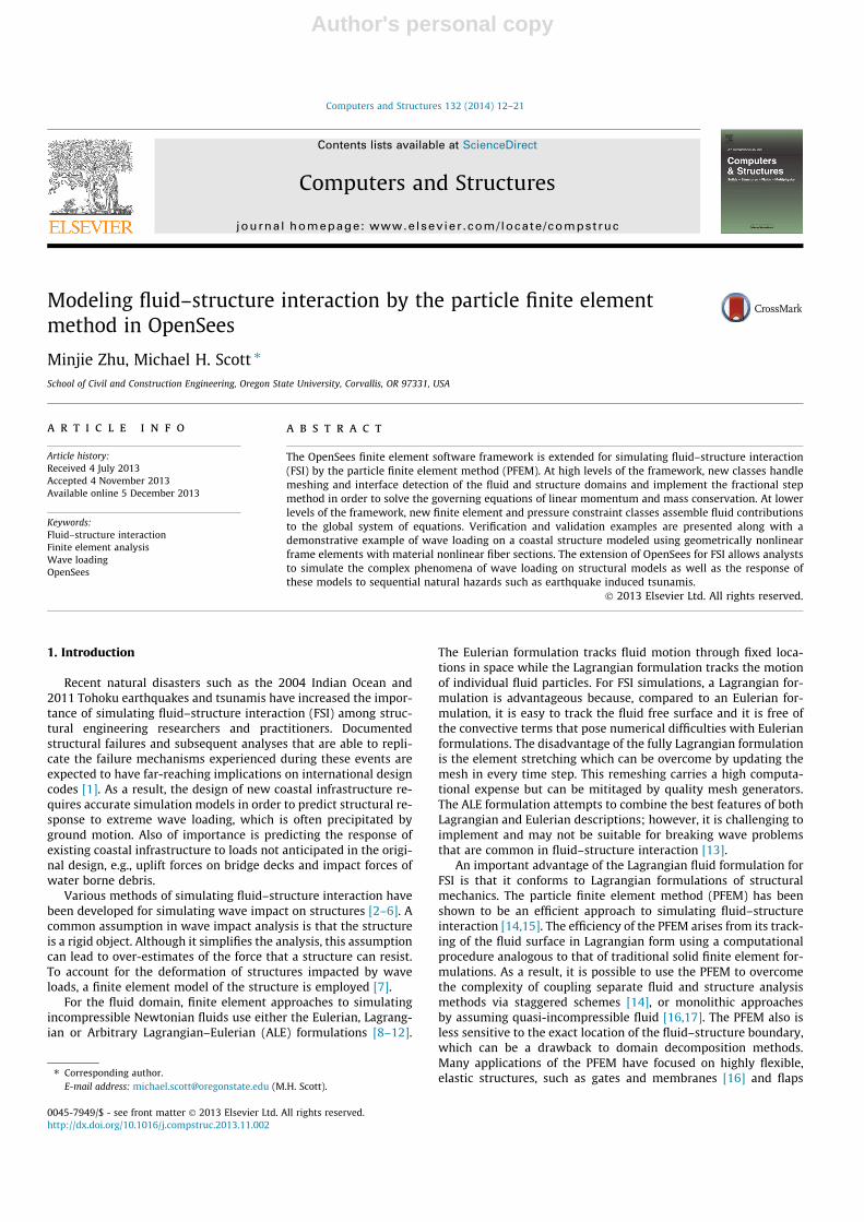
Modeling fluid–structure interaction by the particle finite elementmethod in OpenSees

Minjie Zhu, Michael H. Scott ⇑School of Civil and Construction Engineering, Oregon State University, Corvallis, OR 97331, USA

a r t i c l e i n f o

Article history:Received 4 July 2013Accepted 4 November 2013Available online 5 December 2013

Keywords:Fluid–structure interactionFinite element analysisWave loadingOpenSees

a b s t r a c t

The OpenSees finite element software framework is extended for simulating fluid–structure interaction(FSI) by the particle finite element method (PFEM). At high levels of the framework, new classes handlemeshing and interface detection of the fluid and structure domains and implement the fractional stepmethod in order to solve the governing equations of linear momentum and mass conservation. At lowerlevels of the framework, new finite element and pressure constraint classes assemble fluid contributionsto the global system of equations. Verification and validation examples are presented along with ademonstrative example of wave loading on a coastal structure modeled using geometrically nonlinearframe elements with material nonlinear fiber sections. The extension of OpenSees for FSI allows analyststo simulate the complex phenomena of wave loading on structural models as well as the response ofthese models to sequential natural hazards such as earthquake induced tsunamis.

� 2013 Elsevier Ltd. All rights reserved.

1. Introduction

Recent natural disasters such as the 2004 Indian Ocean and2011 Tohoku earthquakes and tsunamis have increased the impor-tance of simulating fluid–structure interaction (FSI) among struc-tural engineering researchers and practitioners. Documentedstructural failures and subsequent analyses that are able to repli-cate the failure mechanisms experienced during these events areexpected to have far-reaching implications on international designcodes [1]. As a result, the design of new coastal infrastructure re-quires accurate simulation models in order to predict structural re-sponse to extreme wave loading, which is often precipitated byground motion. Also of importance is predicting the response ofexisting coastal infrastructure to loads not anticipated in the origi-nal design, e.g., uplift forces on bridge decks and impact forces ofwater borne debris.

Various methods of simulating fluid–structure interaction havebeen developed for simulating wave impact on structures [2–6]. Acommon assumption in wave impact analysis is that the structureis a rigid object. Although it simplifies the analysis, this assumptioncan lead to over-estimates of the force that a structure can resist.To account for the deformation of structures impacted by waveloads, a finite element model of the structure is employed [7].

For the fluid domain, finite element approaches to simulatingincompressible Newtonian fluids use either the Eulerian, Lagrang-ian or Arbitrary Lagrangian–Eulerian (ALE) formulations [8–12].

The Eulerian formulation tracks fluid motion through fixed loca-tions in space while the Lagrangian formulation tracks the motionof individual fluid particles. For FSI simulations, a Lagrangian for-mulation is advantageous because, compared to an Eulerian for-mulation, it is easy to track the fluid free surface and it is free ofthe convective terms that pose numerical difficulties with Eulerianformulations. The disadvantage of the fully Lagrangian formulationis the element stretching which can be overcome by updating themesh in every time step. This remeshing carries a high computa-tional expense but can be mititaged by quality mesh generators.The ALE formulation attempts to combine the best features of bothLagrangian and Eulerian descriptions; however, it is challenging toimplement and may not be suitable for breaking wave problemsthat are common in fluid–structure interaction [13].

An important advantage of the Lagrangian fluid formulation forFSI is that it conforms to Lagrangian formulations of structuralmechanics. The particle finite element method (PFEM) has beenshown to be an efficient approach to simulating fluid–structureinteraction [14,15]. The efficiency of the PFEM arises from its track-ing of the fluid surface in Lagrangian form using a computationalprocedure analogous to that of traditional solid finite element for-mulations. As a result, it is possible to use the PFEM to overcomethe complexity of coupling separate fluid and structure analysismethods via staggered schemes [14], or monolithic approachesby assuming quasi-incompressible fluid [16,17]. The PFEM also isless sensitive to the exact location of the fluid–structure boundary,which can be a drawback to domain decomposition methods.Many applications of the PFEM have focused on highly flexible,elastic structures, such as gates and membranes [16] and flaps

0045-7949/$ - see front matter � 2013 Elsevier Ltd. All rights reserved.http://dx.doi.org/10.1016/j.compstruc.2013.11.002

⇑ Corresponding author.E-mail address: michael.scott@oregonstate.edu (M.H. Scott).

Computers and Structures 132 (2014) 12–21

Contents lists available at ScienceDirect

Computers and Structures

journal homepage: www.elsevier .com/locate/compstruc

Author's personal copy

and valves [15]. While these components are important for certainapplication spaces, they are not representative of the bridges andbuildings that comprise coastal infrastructure.

The open source finite element software framework OpenSees[18] has been developed to advance research in the simulation ofstructural response to earthquake hazards. A software frameworkdefines the abstract classes from which developers can create con-crete classes that implement specific functionality. The finite ele-ment formulations, constitutive models, and solution algorithmsof the OpenSees framework have been designed in such a way thatapplications not foreseen in the initial framework developmentcan be incorporated with a series of incremental improvementsor additions. For example, the OpenSees framework has been ex-tended to live load rating of bridge girders [19] and to simulatestructural response to fire attack [20].

The objective of this paper is to show how the OpenSees frame-work is extended to accommodate the PFEM for FSI applicationsusing a monolithic approach for fully incompressible fluid. First,the governing equations of the PFEM are presented along withtheir discrete approximations in space and time. Implementationdetails are presented for the new classes added to OpenSees forhandling additional pressure and pressure gradient unknowns atthe element level. Details at the structural level where the solutionfor the pressure unknowns is obtained alongside nodal displace-ments are also presented. Examples of fluid only and FSI are shownin order to verify, validate, and demonstrate the PFEM implemen-tation within OpenSees.

2. Governing equations of the PFEM

A PFEM analysis satisfies conservation of linear momentum andconservation of mass for all points in the fluid and structural do-mains. Constitutive laws relate the displacements at points in thefluid and structural domains to pressure or stress.

2.1. Conservation of linear momentum

Conservation of linear momentum is enforced in the volume, V,of both the fluid and structural domains

q€ui ¼@rij

@xjþ qbi ð1Þ

where €ui is the acceleration vector, rij is the Cauchy stress tensor, xj

is the current position vector, bi is the body force vector, and q is thedensity. Boundary conditions for both domains are enforced for pre-scribed tractions on the surface, Ct ,

rijnj ¼ ti ð2Þ

where ti is the surface traction and nj is the unit normal vector tothe boundary surface. Boundary and initial conditions are imposedon displacements

ui ¼ upi ; ui ¼ u0

i ð3Þ

where upi is the fixed displacement on the boundary and u0

i is theinitial displacement. Initial conditions on velocity, _u0

i , may also beprescribed. As the simulation proceeds, the relationship betweenposition and displacement is

xi ¼ x0i þ ui ð4Þ

where x0i is the initial position.

2.2. Conservation of mass

Mass conservation, or the continuity equation, must be satisfiedin the fluid domain. Assuming incompressible fluid flow, continu-ity requires the divergence of velocity to be zero

@ _ui

@xi¼ 0 ð5Þ

Conservation of mass is satisfied in the structural domain byconstruction.

2.3. Constitutive equations

In the structural domain, the constitutive equations are writtenas a general stress–strain relationship

rij � rijðeklÞ ð6Þ

where ekl is the strain tensor computed from derivatives of the dis-placement field

ekl ¼12

@uk

@xlþ @ul

@xk

� �ð7Þ

The general stress–strain relationship allows for material nonlinearstructural response to external loading.

For an incompressible fluid, the Newtonian constitutive equa-tions are expressed as

rij ¼ Sij � pdij ð8Þ

where dij is the Kronecker delta and p is the pressure. The deviatoricstress tensor, Sij, is defined for linear fluid response as

Sij ¼ 2l _eij ð9Þ

where l is the fluid viscosity and _eij is the strain rate tensor, whichis the time derivative of Eq. (7).

3. Finite element discretization

Discretization of the continuous governing equations of linearmomentum and mass conservation leads to a system of algebraicequations for the displacements and pressures at discrete locationsknown as particles. An additional governing equation is introducedin order to stabilize the conservation of mass equation. Then, theresponse of both the fluid and structural domains is determinedfrom a monolithic system of equations.

3.1. Stabilization of mass equation

For fluid elements that do not satisfy the LBB condition [21,22],spurious pressure modes can be eliminated by augmenting themass conservation equation (Eq. (5)) with stabilizing terms [23–25]

@ _ui

@xi�Xnd

i¼1

s @

@xi

@p@xiþ pi

� �¼ 0 ð10Þ

where nd is the number of spatial dimensions, pi is the pressure gra-dient projection, and s is the stabilization parameter [26]

s ¼ qDtþ 8l

3l2

� ��1

ð11Þ

The variables Dt and l are the simulation time step and characteris-tic element length, respectively.

The pressure gradient projection ensures that the stabilizingterms in Eq. (10) vanish for exact solution of the continuity equa-tion. This gives an additional equation that governs the response offluid particles

M. Zhu, M.H. Scott / Computers and Structures 132 (2014) 12–21 13

Author's personal copy

@p@xiþ pi ¼ 0 ð12Þ

The unknown pressure gradient, pi, must be found at the global le-vel along with the particle displacements and pressures, as de-scribed next.

3.2. Shape functions

Choosing the particle displacement, ui, pressure, p, and pressuregradient, pi, as primary unknowns and applying the standardGalerkin weighted residual method to the momentum equation(1), stabilized mass equation (10), pressure gradient projectionequation (12), and boundary conditions givesZ

Vdui q€ui �

@rij

@xj� qbi

� �dV �

ZCt

duiti dCt ¼ 0 ð13Þ

ZV

q@ _ui

@xidV þ

ZV

Xnd

i¼1

s @q@xi

@p@xiþ pi

� �dV ¼ 0 ð14Þ

ZV

dpis@p@xiþ pi

� �dV ¼ 0 ð15Þ

where dui; q, and dpi are weighting functions that satisfy the essen-tial boundary conditions. The stabilization parameter, s, is intro-duced in Eq. (15) for symmetry with Eq. (14). Boundary termsfrom the integration by parts in Eq. (14) are neglected.

Using standard finite element techniques [7], the displacement,pressure, and pressure gradient are approximated over each ele-ment using equal order linear interpolation

ui ¼Xn

j¼1

Njuji; p ¼

Xn

j¼1

Njpj; pi ¼Xn

j¼1

Njpji ð16Þ

where n is the number of element nodes and Nj are the shape func-tions. For planar analysis with triangle elements, the shape func-tions are equal to the area coordinate of node j. In threedimensions, volume coordinates are used for the shape functionsof tetrahedral elements.

3.3. System of algebraic equations

When assembled over all elements in the fluid domain, the dis-cretized equations for the fluid particle response are expressed inmatrix–vector form as

Mf €uf þ Kf _uf � Gf p ¼ Ff ð17ÞGT

f_uf þ Lpþ Qp ¼ 0 ð18Þ

Q T pþ M̂p ¼ 0 ð19Þ

where uf ;p, and p are vectors that collect the displacement, pres-sure, and pressure gradient of all fluid particles and Ff is the vectorof external forces. The objects Mf and Kf are the mass and stiffnessmatrices, respectively, of the fluid; Gf is the gradient operator; L isthe Laplacian operator; and Q and M̂ are stabilization matrices. Fur-ther information on the discretized fluid equations is found in [24].

The discretized system of equations for dynamic response of thestructural domain is

Ms €us þ Cs _us þ Fints ðusÞ ¼ Fs ð20Þ

where us is the displacement vector of the structural particles (ornodes) and Fs is the external load vector. The static resisting forcevector, Fint

s , is a nonlinear function of the nodal displacements. Likethe mass and damping matrices, Ms and Cs, respectively, the resist-ing force vector is assembled from element contributions.

Particles connected to elements from both the fluid and struc-tural domains are identified as interface particles whose contribu-tions appear in the system of equations for both domains. Fromthe structural domain, equations governing the interface responseare extracted from Eq. (20) and assigned additional i and ssubscripts

Mss €us þMsi €ui þ Css _us þ Csi _ui þ Fints ðus;uiÞ ¼ Fs ð21Þ

Mis €us þMsii€ui þ Cis _us þ Cii _ui þ Fint

i ðus;uiÞ ¼ Fsi ð22Þ

where ui is the displacement vector of the interface nodes. Simi-larly, the interface equations are extracted from Eqs. (17) and (18)for the fluid domain and given additional i and f subscripts

Mff €uf þ Kff _uf � Gf p ¼ Ff ð23ÞMf

ii€ui þ Kii _ui � Gip ¼ Ff

i ð24ÞGT

f_uf þ GT

i_ui þ Lpþ Qp ¼ 0 ð25Þ

Eqs. (22) and (24) are combined in order to solve for the particle re-sponse on the fluid–structure interface.

4. Solution of discretized equations

At each simulation time step, tnþ1, the discretized momentum,pressure, and pressure gradient equations must be solved consid-ering the change in state from the previous time step, tn. The gov-erning equations are posed in residual form then solved via thefractional step method.

4.1. Nonlinear solution algorithm

To utilize a wide range of root finding algorithms, Eqs. (21) and(23) for the structure and fluid response, respectively; Eqs. (22)and (24) for the interface response; and Eqs. (19) and (25) for thepressure and pressure gradient response are combined to givethe following system of residual equations

rs ¼ Fs �Mss €us �Msi €ui � Css _us � Csi _ui � Fints ðus;uiÞ

ri ¼ Fsi þ Ff

i � ðMfii þMs

iiÞ€ui � ðCii þ KiiÞ _ui � Cis _us �Mis €us

� Finti ðus;uiÞ þ Gip

rf ¼ Ff �Mff €uf � Kff _uf þ Gf p

rp ¼ �GTf

_uf � GTi

_ui � Lp� Qp

rp ¼ �Q T p� M̂p

ð26Þ

For simultaneous solution of the preceding equations, all unknownsare collected in a single vector, v, along with the vector, r, of resid-ual equations

v ¼

_us

_ui

_uf

pp

26666664

37777775; r ¼

rs

ri

rf

rp

rp

26666664

37777775

ð27Þ

With an initial guess for the unknowns at the start of the currenttime step, typically the converged state at the previous time step,v0

nþ1 ¼ vn, the incremental update within a simulation time step is

vjþ1nþ1 ¼ vj

nþ1 þ Dvjþ1 ð28Þ

The update is computed according to a Newton algorithm

Dvjþ1 ¼ ðKjTÞ�1

rj ð29Þ

where KjT ¼ �@r=@v is the Jacobian of the residual evaluated at the

current value of the unknowns, vj

14 M. Zhu, M.H. Scott / Computers and Structures 132 (2014) 12–21

Author's personal copy

KT ¼

~KTss~KTsi 0 0 0

~KTis~KTii 0 �Gi 0

0 0 ~KTff �Gf 0

0 GTi GT

f L Q

0 0 0 Q T M̂

266666664

377777775

ð30Þ

Matrices with an over-tilde, e.g., ~KTss, are the algorithmic matricesthat depend on the simulation time step and the chosen time inte-gration method.

Backward Euler time integration is employed here using theparticle velocities as primary unknowns. The displacement andacceleration are expressed in terms of the velocity at the currenttime step and the displacement and velocity at the previous timestep

unþ1 ¼ un þ Dt _unþ1

€unþ1 ¼_unþ1 � _un

Dtð31Þ

Inserting these approximations into the system of algebraic equa-tions leads to the algorithmic matrix for the structural contribution

~KTss ¼1Dt

Mss þ Css þ DtKTss ð32Þ

where KTss ¼ @Fints ðus;uiÞ=@us is the tangent stiffness matrix of the

structure. Analogous definitions for ~KTsi and ~KTis are straightforwardto obtain.

The algorithmic matrix for the fluid contribution is

~KTff ¼1Dt

Mff þ Kff ð33Þ

where Kff can be ignored for small Dt and low fluid viscosity. Thecontribution of the interface nodes to the Jacobian is

~KTii ¼1DtðMf

ii þMsiiÞ þ ðCii þ KiiÞ þ DtKTii ð34Þ

where KTii ¼ @Finti ðus;uiÞ=@ui is the contribution of the tangent stiff-

ness matrix of the structure to the interface particles. Similar to thefluid contribution in Eq. (33), Kii can be ignored for small Dt and lowviscosity.

4.2. Fractional step method

The monolithic matrix in Eq. (30) is ill-conditioned due to cou-pling of the velocity and pressure fields, making it difficult to ob-tain a stable numerical solution for the incremental velocities,pressures, and pressure gradients. To solve for these quantities effi-ciently, the fractional step method (FSM) is utilized [27,28,15]. TheFSM segregates the unknown pressures and velocities into smallersystems of equations that generally are not ill-conditioned. TheFSM can be summarized in three steps:

1. Compute predictor velocities by ignoring pressure contribu-tions arising from Gi and Gf in the first three rows of Eq. (30).

2. Solve for the pressures from the fourth row of Eq. (30) usingadded mass and stiffness from the predicted velocities.

3. Correct the velocities and update the pressure gradients usingthe pressures found in step 2.

Implementation of the FSM requires important changes at highlevels of the OpenSees framework, as described in the followingsection.

5. PFEM implementation in OpenSees

The software design of OpenSees favors object composition overclass inheritance as the mechanism that enables flexibility andextensibility of the framework. At the highest level of the OpenSeesframework, the Domain class contains components (nodes, ele-ments, loads, constraints, etc.) that are created and added to thedomain by a ModelBuilder object through an input script. The stateof each domain component is computed by an Analysis object,which is composed of an equation solver, solution algorithm, timeintegrator, constraint handler, and element and nodal assemblyobjects. Complete details of the design of OpenSees for nonlinearfinite element analysis are given in [29]. Only the details of thePFEM implementation in OpenSees are presented herein.

Since it was primarily designed to solve structural dynamicsproblems, there are two major challenges to the implementationof the PFEM in OpenSees. The first challenge arises from the PFEM’snecessity to update the finite element mesh at every time step dueto large domain changes and changes in the fluid–structure inter-face. While this re-meshing and interface detection can be handledat the script level, it is necessary for efficiency to implement thesemodules within the OpenSees core. The second challenge involvessolving the linear system of equations via the FSM, which requiresmultiple equation solutions using the submatrices in Eq. (30).Although OpenSees contains a flexible set of equation solvers,there is an implicit assumption that only one equation solutiontakes place during each iteration within a time step.

5.1. Meshing and interface detection

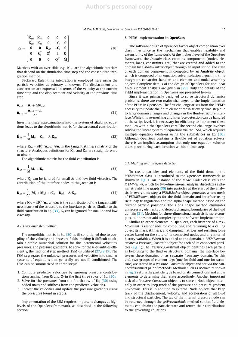
To create particles and elements of the fluid domain, thePFEMMesher class is introduced to the OpenSees framework, asshown in Fig. 1. An instance of the ModelBuilder class calls thePFEMMesher, which for two-dimensional analysis, discretizes a pla-nar straight line graph [30] into particles at the start of the analy-sis. In every time step, a PFEMMesher object generates a new meshof PFEMElement objects for the fluid domain and interface usingDelaunay triangulation and the alpha shape method based on thecurrent particle positions. The alpha shape method eliminatesunnecessary elements and detects changing boundaries of the fluiddomain [31]. Meshing for three-dimensional analysis is more com-plex, but does not add complexity to the software implementation.

Similar to other elements in OpenSees, each instance of a PFE-MElement is responsible for computing and returning to a callingobject its mass, stiffness, and damping matrices and resisting forcevector based on the state of its connected nodes and any internalhistory variables. When it is added to the domain, a PFEMElementcreates a Pressure_Constraint object for each of its connected parti-cles (Fig. 1). The Pressure_Constraint object identifies each particleas belonging to the fluid or structural domains, the interface be-tween these domains, or as separate from any domain. To thisend, two groups of element tags (one for fluid and one for struc-ture) are stored in a Pressure_Constraint object and set via the con-nect/disconnect pair of methods. Methods such as isStructure shownin Fig. 2 return the particle type based on its connections and allowelements to determine their state accordingly. Another importanttask of a Pressure_Constraint object is to store a Node object inter-nally in order to keep track of the pressure and pressure gradientunknowns. This is in addition to external Node objects that keeptrack of the displacement, velocity, and acceleration of all fluidand structural particles. The tag of the internal pressure node canbe returned through the getPressureNode method so that fluid ele-ments can obtain the particle state and return their contributionsto the governing equations.

M. Zhu, M.H. Scott / Computers and Structures 132 (2014) 12–21 15

Author's personal copy

With a fluid mesh in place, the PFEMIntegrator class is able toimplement the implicit Euler time integration method using parti-cle velocity as the primary unknown along with the pressure andpressure gradient. At the start of each time step, the integrator callsPressure_Constraint objects to update the state of each isolated par-ticle and to assemble the governing equations for particles that areconnected to a mesh of fluid elements. The PFEMAnalysis class setsthe maximum and minimum time steps for the simulation andmay reduce the time step if convergence is not achieved.

5.2. Fractional step method

In addition to identifying the domain to which particles belong,the Pressure_Constraint class serves as a bridge between the analy-sis and model classes of OpenSees in order to link the finite ele-ment model to the predictor–corrector approach of the FSM. Onthe analysis side, new implementations of the LinearSOE and Lin-earSolver interfaces shown in Fig. 2 are required in order to carryout the FSM and partition the matrices in Eq. (30) based on themodel information from Pressure_Constraint objects. To this end,the setDofIDs method of the PFEMLinSOE class, which inherits theLinearSOE interface, obtains the node types from the Pressure_Con-straint objects and sets the matrix partitions and assigns equationnumbers. The setMatIDs method is then called in order to initializethe partitioned matrices and residual vector of Eq. (30) for assem-bly via implementations of the addA and addB methods. Using thepartitioned matrices stored in the PFEMLinSOE object, the PFEM-

Solver, which implements the LinearSolver interface, carries outthe FSM and returns the solution for incremental velocities, pres-sures, and pressure gradients.

6. Examples

Examples are presented herein to verify and validate the PFEMimplementation in OpenSees and to demonstrate its application tofluid–structure interaction. Fluid sloshing in a container is used forverification, then collapse of a water column is shown for valida-tion, followed by time history analysis of a coastal structure sub-jected to wave loading. This final example demonstrates howstructural models comprised of frame finite elements and fiber sec-tions (typically employed for earthquake loading) can be subjectedto wave loading via the PFEM implementation in OpenSees.

6.1. Fluid sloshing

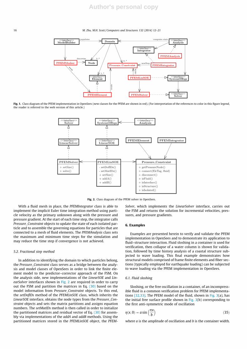
Sloshing, or the free oscillation in a container, of an incompress-ible fluid is a common verification problem for PFEM implementa-tions [32,33]. The PFEM model of the fluid, shown in Fig. 3(a), hasthe initial free surface profile shown in Fig. 3(b) corresponding tothe first anti-symmetric mode of oscillation

gðx;0Þ ¼ a sinpxb

� �ð35Þ

where a is the amplitude of oscillation and b is the container width.

Fig. 1. Class diagram of the PFEM implementation in OpenSees (new classes for the PFEM are shown in red). (For interpretation of the references to color in this figure legend,the reader is referred to the web version of this article.)

Fig. 2. Class diagram of the PFEM solver in OpenSees.

16 M. Zhu, M.H. Scott / Computers and Structures 132 (2014) 12–21

Author's personal copy

Fig. 3. Initial mesh for fluid sloshing problem.

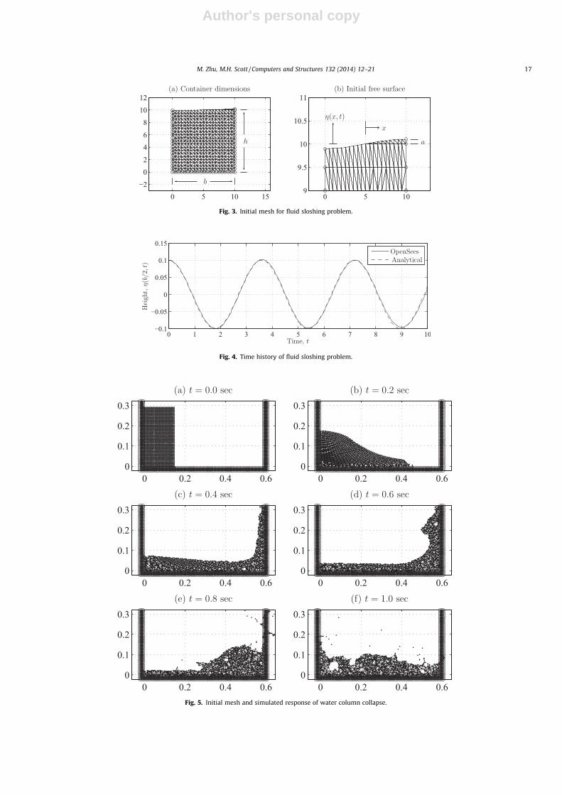
Fig. 4. Time history of fluid sloshing problem.

Fig. 5. Initial mesh and simulated response of water column collapse.

M. Zhu, M.H. Scott / Computers and Structures 132 (2014) 12–21 17

Author's personal copy

When the amplitude is small compared to the container height,h, the analytical solution for the motion of the free surface is

gðx; tÞ ¼ a sinpxb

� �cosðrtÞ ð36Þ

The frequency of oscillation, r, is calculated from the dispersionrelationship

r2 ¼ pgb

tanhphb

� �ð37Þ

where g is the gravitational constant.For numerical simulation via the PFEM, the mesh shown in

Fig. 3(a) with container dimensions, b ¼ h ¼ 10 m, and amplitude,a ¼ 0:1 m, has 453 nodes and 819 elements. The simulation timestep is Dt ¼ 0:001 s. The sloshing time history of the free surfaceat x ¼ b=2 is shown in Fig. 4. The simulation results agree withthe closed form solution save for the numerical approximation ofthe implicit Euler time integration.

6.2. Water column collapse

Where the sloshing time history provided verification using aclosed-form solution of steady state response, the collapse of awater column is a standard example for validation of Lagrangian

formulations of fluid flow undergoing highly nonlinear mesh dis-tortions [32]. The initial configuration of the water column isshown in Fig. 5(a) with 1392 nodes and 2429 elements. Using asimulation time step of Dt ¼ 0:001 s, the evolution of the free sur-face shown in Fig. 5(b)–(f) agrees qualitatively with previouslypublished results [32,34].

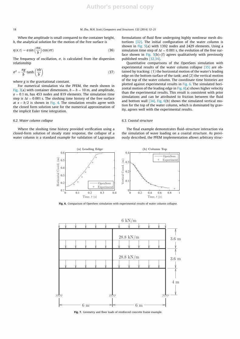
Quantitative comparisons of the OpenSees simulation withexperimental results of the water column collapse [35] are ob-tained by tracking: (1) the horizontal motion of the water’s leadingedge on the bottom surface of the tank; and (2) the vertical motionof the top of the water column. The coordinate time histories areplotted against experimental results in Fig. 6. The simulated hori-zontal motion of the leading edge in Fig. 6(a) shows higher velocitythan the experimental results. This result is consistent with priorsimulations and can be attributed to friction between the fluidand bottom wall [34]. Fig. 6(b) shows the simulated vertical mo-tion for the top of the water column, which is dominated by grav-ity, agrees well with the experimental results.

6.3. Coastal structure

The final example demonstrates fluid–structure interaction viathe simulation of wave loading on a coastal structure. As previ-ously described, the PFEM implementation allows arbitrary struc-

Fig. 6. Comparison of OpenSees simulation with experimental results of water column collapse.

Fig. 7. Geometry and floor loads of reinforced concrete frame example.

18 M. Zhu, M.H. Scott / Computers and Structures 132 (2014) 12–21

Author's personal copy

tural finite elements to be used so that the existing modules ofOpenSees can be exploited for detailed analyses. Although the sim-ulation does not capture essential three-dimensional FSI effects, itdemonstrates the capabilities.

The structural model is of the interior frame of a reinforced con-crete building analyzed by Madurapperuma and Wijeyewickrema[36] for impact of water borne debris (see Fig. 7). Dead load onall members consists of self-weight and beam live loads were com-puted assuming uniform 4.8 kPa on floor slabs and 1.0 kPa on theroof with tributary width of 6 m. Combined dead and live loadwere used in assigning lumped masses to the frame nodes. Theframe members are discretized into ten displacement-based framefinite elements, each with constant axial strain and linear curva-ture approximations (dispBeamColumn in OpenSees). Althoughframe finite elements typically use a relatively coarse mesh, theresulting element lengths are comparable to the characteristic sizeof the fluid mesh so that a complete fluid–structure interface isdeveloped during the simulation. The corotational transformation[37] captures geometric nonlinear response of the frame.

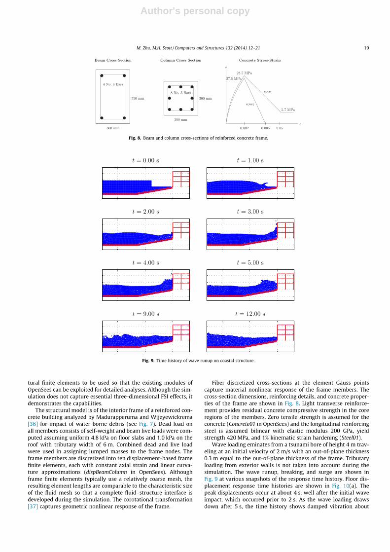
Fiber discretized cross-sections at the element Gauss pointscapture material nonlinear response of the frame members. Thecross-section dimensions, reinforcing details, and concrete proper-ties of the frame are shown in Fig. 8. Light transverse reinforce-ment provides residual concrete compressive strength in the coreregions of the members. Zero tensile strength is assumed for theconcrete (Concrete01 in OpenSees) and the longitudinal reinforcingsteel is assumed bilinear with elastic modulus 200 GPa, yieldstrength 420 MPa, and 1% kinematic strain hardening (Steel01).

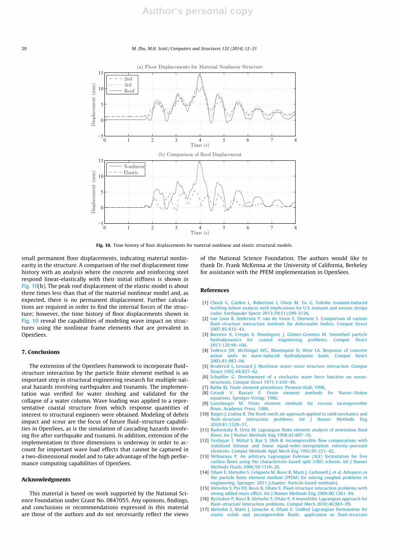
Wave loading eminates from a tsunami bore of height 4 m trav-eling at an initial velocity of 2 m/s with an out-of-plane thickness0.3 m equal to the out-of-plane thickness of the frame. Tributaryloading from exterior walls is not taken into account during thesimulation. The wave runup, breaking, and surge are shown inFig. 9 at various snapshots of the response time history. Floor dis-placement response time histories are shown in Fig. 10(a). Thepeak displacements occur at about 4 s, well after the initial waveimpact, which occurred prior to 2 s. As the wave loading drawsdown after 5 s, the time history shows damped vibration about

Fig. 8. Beam and column cross-sections of reinforced concrete frame.

Fig. 9. Time history of wave runup on coastal structure.

M. Zhu, M.H. Scott / Computers and Structures 132 (2014) 12–21 19

Author's personal copy

small permanent floor displacements, indicating material nonlin-earity in the structure. A comparison of the roof displacement timehistory with an analysis where the concrete and reinforcing steelrespond linear-elastically with their initial stiffness is shown inFig. 10(b). The peak roof displacement of the elastic model is aboutthree times less than that of the material nonlinear model and, asexpected, there is no permanent displacement. Further calcula-tions are required in order to find the internal forces of the struc-ture; however, the time history of floor displacements shown inFig. 10 reveal the capabilities of modeling wave impact on struc-tures using the nonlinear frame elements that are prevalent inOpenSees.

7. Conclusions

The extension of the OpenSees framework to incorporate fluid–structure interaction by the particle finite element method is animportant step in structural engineering research for multiple nat-ural hazards involving earthquakes and tsunamis. The implemen-tation was verified for water sloshing and validated for thecollapse of a water column. Wave loading was applied to a repre-sentative coastal structure from which response quantities ofinterest to structural engineers were obtained. Modeling of debrisimpact and scour are the focus of future fluid–structure capabili-ties in OpenSees, as is the simulation of cascading hazards involv-ing fire after earthquake and tsunami. In addition, extension of theimplementation to three dimensions is underway in order to ac-count for important wave load effects that cannot be captured ina two-dimensional model and to take advantage of the high perfor-mance computing capabilities of OpenSees.

Acknowledgments

This material is based on work supported by the National Sci-ence Foundation under Grant No. 0847055. Any opinions, findings,and conclusions or recommendations expressed in this materialare those of the authors and do not necessarily reflect the views

of the National Science Foundation. The authors would like tothank Dr. Frank McKenna at the University of California, Berkeleyfor assistance with the PFEM implementation in OpenSees.

References

[1] Chock G, Carden L, Robertson I, Olsen M, Yu G. Tohoku tsunami-inducedbuilding failure analysis with implications for U.S. tsunami and seismic designcodes. Earthquake Spectr 2013;29(S1):S99–S126.

[2] van Loon R, Anderson P, van de Vosse F, Sherwin S. Comparison of variousfluid–structure interaction methods for deformable bodies. Comput Struct2007;85:833–43.

[3] Barreiro A, Crespo A, Domínguez J, Gómez-Gesteira M. Smoothed particlehydrodynamics for coastal engineering problems. Comput Struct2013;120:96–106.

[4] Tedesco JW, McDougal WG, Bloomquist D, Wise LA. Response of concretearmor units to wave-induced hydrodynamic loads. Comput Struct2003;81:983–94.

[5] Broderick L, Leonard J. Nonlinear water–wave structure interaction. ComputStruct 1992;44:837–42.

[6] Schuëller G. Development of a stochastic wave force function on ocean-structures. Comput Struct 1971;1:639–49.

[7] Bathe KJ. Finite element procedures. Prentice-Hall; 1996.[8] Girault V, Raviart P. Finite element methods for Navier–Stokes

equations. Springer-Verlag; 1986.[9] Gunzburger M. Finite element methods for viscous incompressible

flows. Academic Press; 1989.[10] Baiges J, Codina R. The fixed-mesh ale approach applied to solid mechanics and

fluid–structure interaction problems. Int J Numer Methods Eng2010;81:1529–57.

[11] Radovitzky R, Ortiz M. Lagrangian finite element analysis of newtonian fluidflows. Int J Numer Methods Eng 1998;43:607–19.

[12] Tezduyar T, Mittal S, Ray S, Shih R. Incompressible flow computations withstabilized bilinear and linear equal-order-interpolation velocity–pressureelements. Comput Methods Appl Mech Eng 1992;95:221–42.

[13] Nithiarasu P. An arbitrary Lagrangian Eulerian (ALE) formulation for freesurface flows using the characteristic-based split (CBS) scheme. Int J NumerMethods Fluids 2006;50:1119–20.

[14] Oñate E, Idelsohn S, Celigueta M, Rossi R, Marti J, Carbonell J, et al. Advances inthe particle finite element method (PFEM) for solving coupled problems inengineering. Springer; 2011 [chapter: Particle-based methods].

[15] Idelsohn S, Pin FD, Rossi R, Oñate E. Fluid-structure interaction problems withstrong added-mass effect. Int J Numer Methods Eng 2009;80:1261–94.

[16] Ryzhakov P, Rossi R, Idelsohn S, Oñate E. A monolithic Lagrangian approach forfluid–structure interaction problems. Comput Mech 2010;46:883–99.

[17] Idelsohn S, Marti J, Limache A, Oñate E. Unified Lagrangian formulation forelastic solids and incompressible fluids: application to fluid-structure

Fig. 10. Time history of floor displacements for material nonlinear and elastic structural models.

20 M. Zhu, M.H. Scott / Computers and Structures 132 (2014) 12–21

Author's personal copy

interaction problems via the PFEM. Comput Methods Appl Mech Eng2008;197:1762–76.

[18] McKenna F, Fenves GL, Scott MH. Open system for earthquake engineeringsimulation. Berkeley, CA: University of California; 2000. Available from:<http://opensees.berkeley.edu>.

[19] Scott MH, Kidarsa A, Higgins C. Development of bridge rating applicationsusing OpenSees and Tcl. J Comput Civil Eng 2008;22(4):264–71.

[20] Jiang J, Usmani A. Modeling of steel frame structures in fire using OpenSees.Comput Struct 2013;118:90–9.

[21] Donea J, Huerta A. Finite element methods for flow problems. John Wiley;2003.

[22] Gresho PM, Sani RL, Engelman MS. Incompressible flow and the finite elementmethod: advection–diffusion and isothermal laminar flow. John Wiley andSons; 1998.

[23] Oñate E. A stabilized finite element method for incompressible viscous flowsusing a finite increment calculus formulation. Comput Methods Appl MechEng 2000;182:355–70.

[24] Oñate E, Garcia J, Idelsohn S, Pin FD. Finite calculus formulations for finiteelement analysis of incompressible flows. Eulerian, ale and Lagrangianapproaches. Comput Methods Appl Mech Eng 2006;195:3001–37.

[25] Oñate E, Nadukandi P, Idelsohn SR, García J, Felippa C. A family of residual-based stabilized finite element methods for stokes flow. Int J Numer MethodsFluids 2011;65:106–34.

[26] Oñate E, Idelsohn SR, Felippa CA. Consistent pressure Laplacian stabilizationfor incompressible continua via higher-order finite calculus. Int J NumerMethods Eng 2011;87:171–95.

[27] Idelsohn SR, Oñate E. The challenge of mass conservation in the solution offree-surface flows with the fractional-step method: problems and solutions.Int J Numer Methods Biomed Eng 2010;26:1313–30.

[28] Aubry R, Idelsohn S, Oñate E. Fractional step like schemes for free surfaceproblems with thermal coupling using the Lagrangian PFEM. Comput Mech2006;38:294–309.

[29] McKenna F, Scott MH, Fenves GL. Nonlinear finite-element analysis softwarearchitecture using object composition. J Comput Civil Eng 2010;24(1):95–107.

[30] Shewchuk JR. Triangle: engineering a 2D quality mesh generator and delaunaytriangulator. In: Lin MC, Manocha D, editors. Applied computational geometry:towards geometric engineering. Lecture notes in computer science, vol.1148. Springer-Verlag; 1996. p. 203–22 [from the first ACM workshop onapplied computational geometry].

[31] Edelsbrunner H, Mücke EP. Three-dimensional alpha shapes. ACM TransGraphics 1994;13(1):43–72.

[32] Oñate E, Idelsohn S, Pin FD, Aubry R. The particle finite element method anoverview. Int J Comput Methods 2004;1(2):267–307.

[33] Cremonesi M, Frangi A, Perego U. A lagrangian finite element approach for theanalysis of fluid–structure interaction problems. Int J Numer Methods Eng2010;84:610–30.

[34] Koshizuka S, Oka Y. Moving-particle semi-implicit method for fragmentationof incompressible fluid. Nucl Sci Eng 1996;123:421–34.

[35] Martin J, Moyce WJ. An experimental study of the collapse of liquid columnson a rigid horizontal plane. Philos Trans R Soc London Ser A Math Phys Sci1952;244(882):312–24.

[36] Madurapperuma MAKM, Wijeyewickrema AC. Inelastic dynamic analysis of anRC building impacted by a tsunami water-borne shipping container. JEarthquake Tsunami 2012;6(1):12500011–017.

[37] Crisfield MA. Non-linear finite element analysis of solids and structures, vol.1. John Wiley & Sons; 1991.

M. Zhu, M.H. Scott / Computers and Structures 132 (2014) 12–21 21

View publication statsView publication stats