The Open Geology Journal, 2010, 4, 29-34 29

1874-2629/10 2010 Bentham Open

Open Access

Numerical Analysis of Historic Gold Production Cycles and Implications for Future Sub-Cycles

J. Müller*,1 and H.E. Frimmel2,3

1Faculty of Mining and Geology, Technical University of Ostrava, 17.listopadu 15/2172, Ostrava-Poruba, 708 33,

Czech Republic, and Einkaufsgemeinschaft für Gold und Silber GbR, Gartenstrasse 28, D-89547 Gerstetten, Germany

2Geodynamics & Geomaterials Research Division, University of Würzburg, Am Hubland, D-97074 Würzburg, Germany

3Department of Geological Sciences, University of Cape Town, Rondebosch 7701, South Africa

Abstract: Gold production at an industrial scale developed with the discovery of gold in Australia and the USA in the middle of the 19th century. Since then the gold production rose exponentially with a rate of approximately 2.0% thus reflecting a first-order production cycle. Within this rise, however, four individual sub-cycles can be identified. The current sub-cycle is predicted to lead from a peak in 2001 of 2,600 tons to a global production of 1,600 tons in the year 2018 or even as little as 780 tons in 2026. Further analysis of these sub-cycles, consideration of declining ore grades and energetic constraints lead us to suggest that the year 2001 indeed could have been the peak-gold year of the main 'Hubbert-style' production cycle. A cumulative achievable gold production between 230,000 and 280,000 tons is derived from the application of the so-called Hubbert Linearization. This compares well with a minimum of about 285,000 tons of combined past production and known reserves and resources.

Keywords: Global gold production cycle, Hubbert Linearization, peak gold.

INTRODUCTION

Since the beginning of the industrial era of gold production at around 1850, 148,000 tons of gold were produced. Estimates of the historic cumulative production ranges from 157,000 tons [1] to 180,000 tons [2]. Thus, between 82% and 94% of the historic production was mined within the last 160 years. South Africa alone contributed with approximately 50,000 tons about one third of the global production. However, reasonably well documented global production figures only date back to the end of the 15th century [3]. The U.S. Geological Survey estimates that 85% of all historically produced gold is still available for recycling [1], i.e. between 133,000 and 153,000 tons.

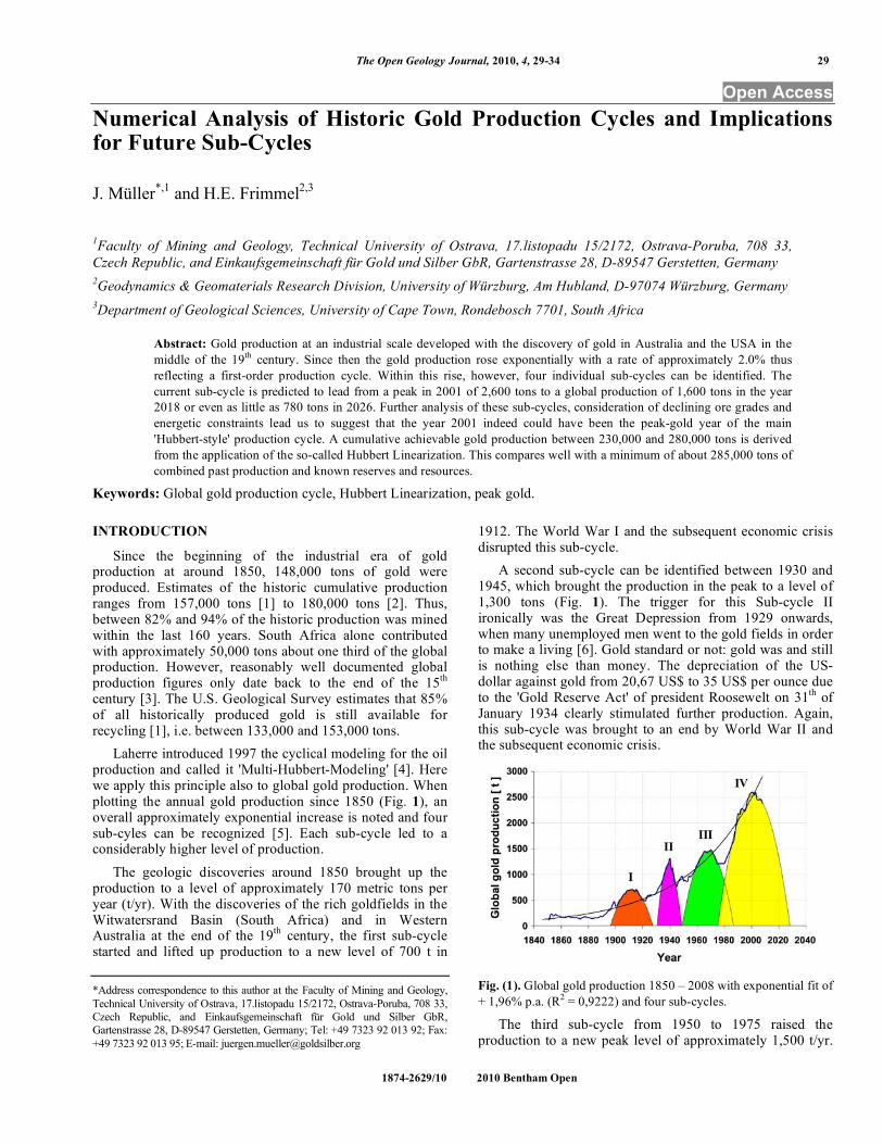
Laherre introduced 1997 the cyclical modeling for the oil production and called it 'Multi-Hubbert-Modeling' [4]. Here we apply this principle also to global gold production. When plotting the annual gold production since 1850 (Fig. 1), an overall approximately exponential increase is noted and four sub-cyles can be recognized [5]. Each sub-cycle led to a considerably higher level of production.

The geologic discoveries around 1850 brought up the production to a level of approximately 170 metric tons per year (t/yr). With the discoveries of the rich goldfields in the Witwatersrand Basin (South Africa) and in Western Australia at the end of the 19th century, the first sub-cycle started and lifted up production to a new level of 700 t in

*Address correspondence to this author at the Faculty of Mining and Geology, Technical University of Ostrava, 17.listopadu 15/2172, Ostrava-Poruba, 708 33, Czech Republic, and Einkaufsgemeinschaft für Gold und Silber GbR, Gartenstrasse 28, D-89547 Gerstetten, Germany; Tel: +49 7323 92 013 92; Fax: +49 7323 92 013 95; E-mail: juergen.mueller@goldsilber.org

1912. The World War I and the subsequent economic crisis disrupted this sub-cycle.

A second sub-cycle can be identified between 1930 and 1945, which brought the production in the peak to a level of 1,300 tons (Fig. 1). The trigger for this Sub-cycle II ironically was the Great Depression from 1929 onwards, when many unemployed men went to the gold fields in order to make a living [6]. Gold standard or not: gold was and still is nothing else than money. The depreciation of the US-dollar against gold from 20,67 US$ to 35 US$ per ounce due to the 'Gold Reserve Act' of president Roosewelt on 31th of January 1934 clearly stimulated further production. Again, this sub-cycle was brought to an end by World War II and the subsequent economic crisis.

Fig. (1). Global gold production 1850 – 2008 with exponential fit of + 1,96% p.a. (R2 = 0,9222) and four sub-cycles.

The third sub-cycle from 1950 to 1975 raised the production to a new peak level of approximately 1,500 t/yr.

30 The Open Geology Journal, 2010, Volume 4 Müller and Frimmel

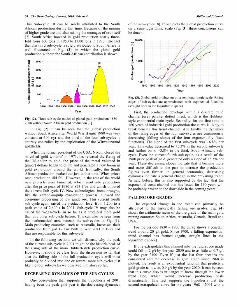
This Sub-cycle III can be solely attributed to the South African production during that time. Because of the mining of higher grade ore and also raising the tonnages of ore itself [7], South Africa boosted its gold production nearly three-fold from 360 tons in 1950 to 1,000 tons in 1970. The fact that this third sub-cycle is solely attributed to South Africa is well illustrated in Fig. (2), in which the global gold production without the South African contribution is shown.

Fig. (2). Three-sub-cycle model of global gold production 1850 – 2008 without South African gold production [7].

In Fig. (2) it can be seen that the global production without South Africa after World War II until 1980 was very constant at 500 t/yr and the third of the four sub-cycles is entirely controlled by the exploitation of the Witwatersrand goldfields.

When the former president of the USA, Nixon, closed the so called 'gold window' in 1971, i.e. released the fixing of the US-dollar to gold, the price of the metal valuated in (paper) dollars began to climb and generated a new boom in gold exploration around the world. Ironically, the South African production peaked out just at that time. When prices rose, production did fall. However, in the rest of the world new projects were launched, which went into production after the price peak of 1980 at 873 $/oz and which initiated the current Sub-cycle IV. New technological breakthroughs, like the carbon-in-pulp cyanidation process, allowed the economic processing of low grade ore. This current fourth sub-cycle again raised the production level from 1,200 to a peak value of 2,600 t in 2001. Sub-cycle IV may also be called the 'mega-cycle' in so far as it produced more gold than any other sub-cycle before. This can also be seen from the mathematical area beneath the sub-cycles in Fig. (1). Main producing countries, such as Australia, increased their production from just 17 t in 1980 to over 310 t in 1997 and thus are responsible for this sub-cycle.

In the following sections we will discuss, why the peak of the current sub-cycle in 2001 might be the historic peak of the rising side of the main Hubbert-style production curve. However, it should be clear from the discussion so far that also the falling side of the full production cycle will most probably be divided into one or several more sub-cycles just like the four sub-cycles we observed in history so far.

DECREASING DYNAMICS OF THE SUB-CYCLES

One observation that supports the hypothesis of 2001 having been the peak-gold year is the decreasing dynamics

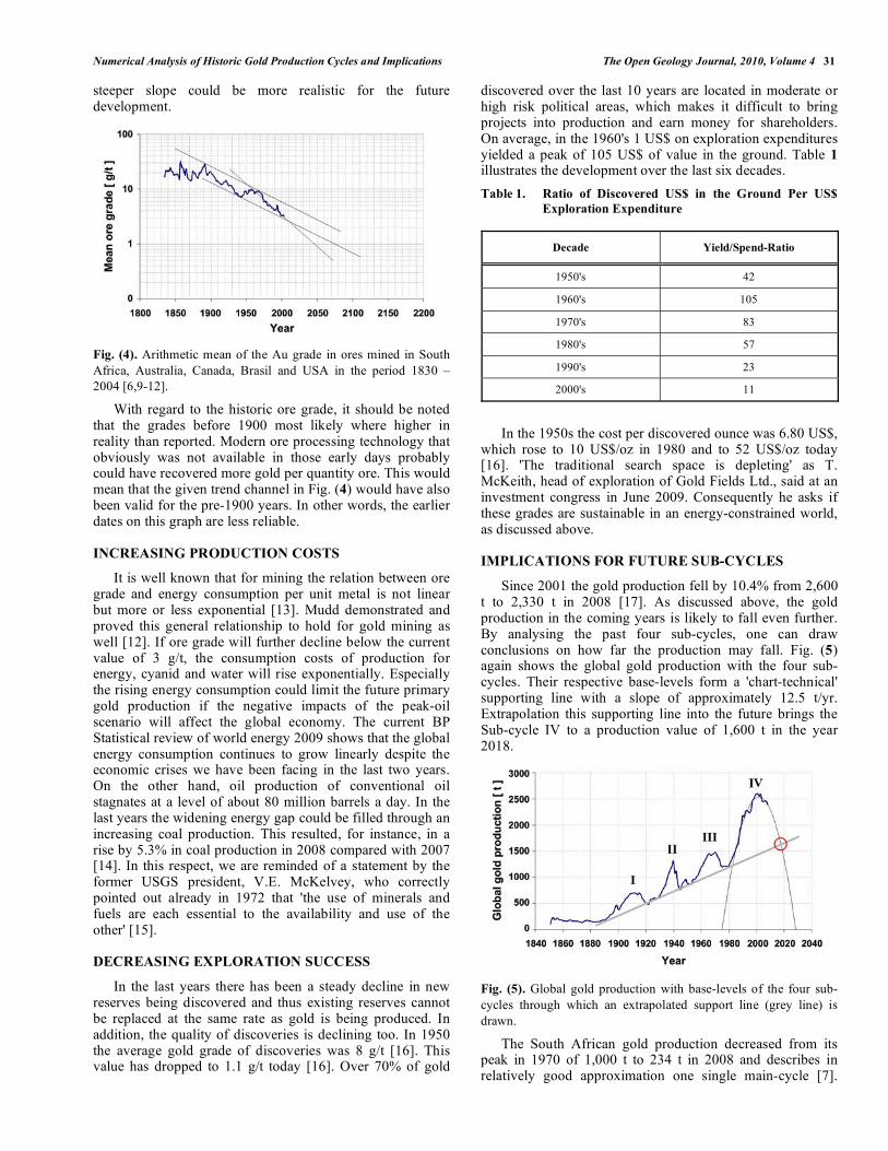
of the sub-cycles [8]. If one plots the global production curve on a semi-logarithmic scale (Fig. 3), three conclusions can be drawn.

Fig. (3). Global gold production on a semilogarithmic scale. Rising edges of sub-cycles are approximated with exponential functions (straight lines in the logarithmic space).

First, the production develops within a discrete trend channel (grey parallel dotted lines), which is the Hubbert-style exponential main-cycle. Secondly, for the first time in 160 years of industrial gold production the curve is likely to break beneath this trend channel. And finally the dynamics of the rising edges of the four sub-cycles are continuously decreasing (falling slopes of the four exponentially fitted functions). The slope of the first sub-cycle was +6.8% per year. This value decreased to +5.3% in the second sub-cycle and further on to +3.8% in the third, 'South-African', sub-cycle. Even the current fourth sub-cycle, as a result of the 1980 price peak of gold, generated only a slope of +3.3% per year. These decreasing slopes indicate that it became more and more difficult in the past to increase the production figures even further. In general economics, decreasing dynamics indicate a general change in the prevailing trend. As said before, this is also supported by the fact that the exponential trend channel that has lasted for 160 years will be probably broken to the downside in the coming years.

FALLING ORE GRADES

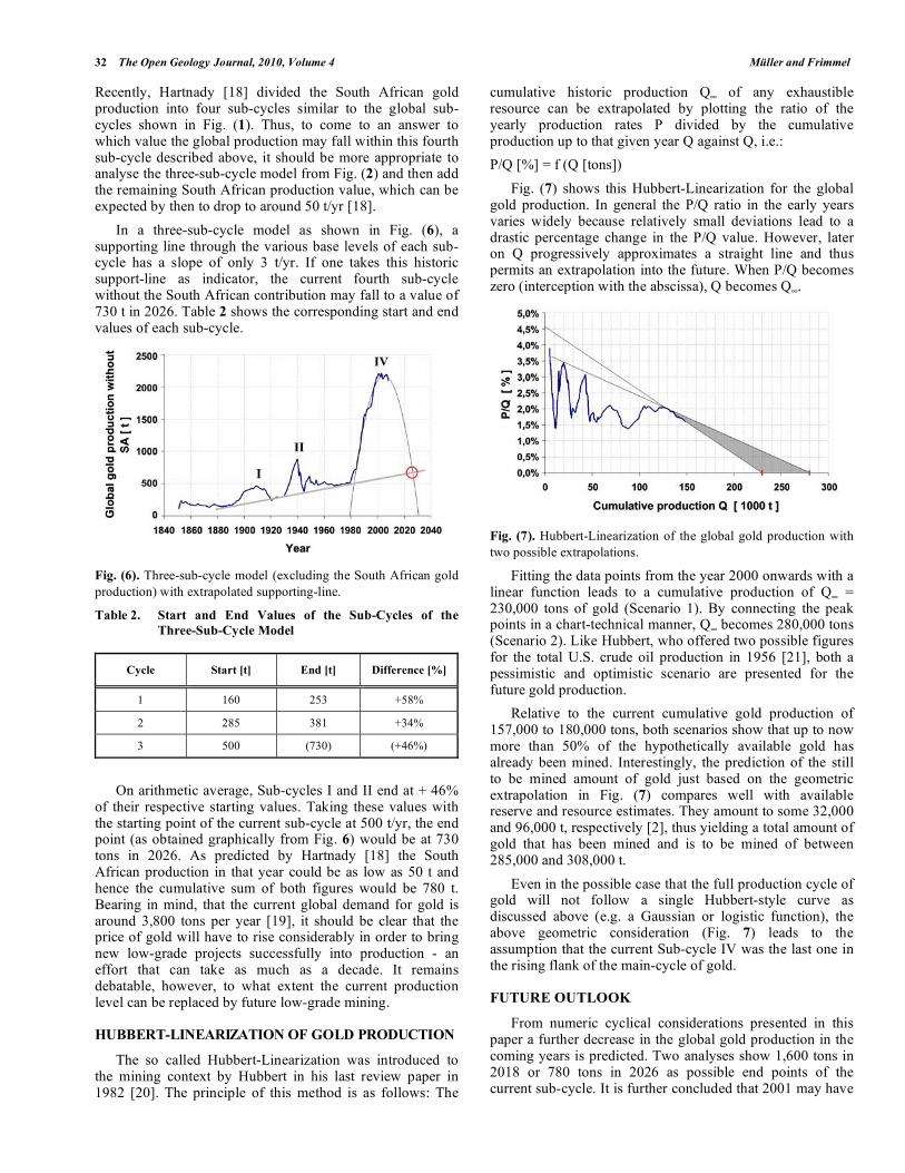
The expected change in the trend can primarily be attributed to the historically falling ore grades. Fig. (4) shows the arithmetic mean of the ore grade of the main gold mining countries South Africa, Australia, Canada, Brasil and USA.

For the periode 1830 – 1900 the curve shows a constant trend around 20 g/t gold. Since 1900, a falling exponential trend channel has formed (again, straight lines in the logarithmic space).

If one extrapolates this channel into the future, ore grade could fall to 2 g/t by the year 2050 and to as little as 0.7 g/t by the year 2100. Even if just the last four decades are considered and the decrease in gold grade since 1968 is plotted, the result is an exponential function that predicts a gold grade as low as 0.9 g/t by the year 2050. It can be seen that this curve also is in danger to break through the lower trend line, which would increase production costs dramatically. This fact supports the hypothesis that the second extrapolated curve for the years 1968 – 2004 with a

Numerical Analysis of Historic Gold Production Cycles and Implications The Open Geology Journal, 2010, Volume 4 31

steeper slope could be more realistic for the future development.

Fig. (4). Arithmetic mean of the Au grade in ores mined in South Africa, Australia, Canada, Brasil and USA in the period 1830 – 2004 [6,9-12].

With regard to the historic ore grade, it should be noted that the grades before 1900 most likely where higher in reality than reported. Modern ore processing technology that obviously was not available in those early days probably could have recovered more gold per quantity ore. This would mean that the given trend channel in Fig. (4) would have also been valid for the pre-1900 years. In other words, the earlier dates on this graph are less reliable.

INCREASING PRODUCTION COSTS

It is well known that for mining the relation between ore grade and energy consumption per unit metal is not linear but more or less exponential [13]. Mudd demonstrated and proved this general relationship to hold for gold mining as well [12]. If ore grade will further decline below the current value of 3 g/t, the consumption costs of production for energy, cyanid and water will rise exponentially. Especially the rising energy consumption could limit the future primary gold production if the negative impacts of the peak-oil scenario will affect the global economy. The current BP Statistical review of world energy 2009 shows that the global energy consumption continues to grow linearly despite the economic crises we have been facing in the last two years. On the other hand, oil production of conventional oil stagnates at a level of about 80 million barrels a day. In the last years the widening energy gap could be filled through an increasing coal production. This resulted, for instance, in a rise by 5.3% in coal production in 2008 compared with 2007 [14]. In this respect, we are reminded of a statement by the former USGS president, V.E. McKelvey, who correctly pointed out already in 1972 that 'the use of minerals and fuels are each essential to the availability and use of the other' [15].

DECREASING EXPLORATION SUCCESS

In the last years there has been a steady decline in new reserves being discovered and thus existing reserves cannot be replaced at the same rate as gold is being produced. In addition, the quality of discoveries is declining too. In 1950 the average gold grade of discoveries was 8 g/t [16]. This value has dropped to 1.1 g/t today [16]. Over 70% of gold

discovered over the last 10 years are located in moderate or high risk political areas, which makes it difficult to bring projects into production and earn money for shareholders. On average, in the 1960's 1 US$ on exploration expenditures yielded a peak of 105 US$ of value in the ground. Table 1 illustrates the development over the last six decades.

Table 1. Ratio of Discovered US$ in the Ground Per US$

Exploration Expenditure

Decade Yield/Spend-Ratio

1950's 42

1960's 105

1970's 83

1980's 57

1990's 23

2000's 11

In the 1950s the cost per discovered ounce was 6.80 US$, which rose to 10 US$/oz in 1980 and to 52 US$/oz today [16]. 'The traditional search space is depleting' as T. McKeith, head of exploration of Gold Fields Ltd., said at an investment congress in June 2009. Consequently he asks if these grades are sustainable in an energy-constrained world, as discussed above.

IMPLICATIONS FOR FUTURE SUB-CYCLES

Since 2001 the gold production fell by 10.4% from 2,600 t to 2,330 t in 2008 [17]. As discussed above, the gold production in the coming years is likely to fall even further. By analysing the past four sub-cycles, one can draw conclusions on how far the production may fall. Fig. (5) again shows the global gold production with the four sub-cycles. Their respective base-levels form a 'chart-technical' supporting line with a slope of approximately 12.5 t/yr. Extrapolation this supporting line into the future brings the Sub-cycle IV to a production value of 1,600 t in the year 2018.

Fig. (5). Global gold production with base-levels of the four sub-cycles through which an extrapolated support line (grey line) is drawn.

The South African gold production decreased from its peak in 1970 of 1,000 t to 234 t in 2008 and describes in relatively good approximation one single main-cycle [7].

32 The Open Geology Journal, 2010, Volume 4 Müller and Frimmel

Recently, Hartnady [18] divided the South African gold production into four sub-cycles similar to the global sub-cycles shown in Fig. (1). Thus, to come to an answer to which value the global production may fall within this fourth sub-cycle described above, it should be more appropriate to analyse the three-sub-cycle model from Fig. (2) and then add the remaining South African production value, which can be expected by then to drop to around 50 t/yr [18].

In a three-sub-cycle model as shown in Fig. (6), a supporting line through the various base levels of each sub-cycle has a slope of only 3 t/yr. If one takes this historic support-line as indicator, the current fourth sub-cycle without the South African contribution may fall to a value of 730 t in 2026. Table 2 shows the corresponding start and end values of each sub-cycle.

Fig. (6). Three-sub-cycle model (excluding the South African gold production) with extrapolated supporting-line.

Table 2. Start and End Values of the Sub-Cycles of the

Three-Sub-Cycle Model

Cycle Start [t] End [t] Difference [%]

1 160 253 +58%

2 285 381 +34%

3 500 (730) (+46%)

On arithmetic average, Sub-cycles I and II end at + 46% of their respective starting values. Taking these values with the starting point of the current sub-cycle at 500 t/yr, the end point (as obtained graphically from Fig. 6) would be at 730 tons in 2026. As predicted by Hartnady [18] the South African production in that year could be as low as 50 t and hence the cumulative sum of both figures would be 780 t. Bearing in mind, that the current global demand for gold is around 3,800 tons per year [19], it should be clear that the price of gold will have to rise considerably in order to bring new low-grade projects successfully into production - an effort that can take as much as a decade. It remains debatable, however, to what extent the current production level can be replaced by future low-grade mining.

HUBBERT-LINEARIZATION OF GOLD PRODUCTION

The so called Hubbert-Linearization was introduced to the mining context by Hubbert in his last review paper in 1982 [20]. The principle of this method is as follows: The

cumulative historic production Q of any exhaustible resource can be extrapolated by plotting the ratio of the yearly production rates P divided by the cumulative production up to that given year Q against Q, i.e.:

P/Q [%] = f (Q [tons])

Fig. (7) shows this Hubbert-Linearization for the global gold production. In general the P/Q ratio in the early years varies widely because relatively small deviations lead to a drastic percentage change in the P/Q value. However, later on Q progressively approximates a straight line and thus permits an extrapolation into the future. When P/Q becomes zero (interception with the abscissa), Q becomes Q .

Fig. (7). Hubbert-Linearization of the global gold production with two possible extrapolations.

Fitting the data points from the year 2000 onwards with a linear function leads to a cumulative production of Q = 230,000 tons of gold (Scenario 1). By connecting the peak points in a chart-technical manner, Q becomes 280,000 tons (Scenario 2). Like Hubbert, who offered two possible figures for the total U.S. crude oil production in 1956 [21], both a pessimistic and optimistic scenario are presented for the future gold production.

Relative to the current cumulative gold production of 157,000 to 180,000 tons, both scenarios show that up to now more than 50% of the hypothetically available gold has already been mined. Interestingly, the prediction of the still to be mined amount of gold just based on the geometric extrapolation in Fig. (7) compares well with available reserve and resource estimates. They amount to some 32,000 and 96,000 t, respectively [2], thus yielding a total amount of gold that has been mined and is to be mined of between 285,000 and 308,000 t.

Even in the possible case that the full production cycle of gold will not follow a single Hubbert-style curve as discussed above (e.g. a Gaussian or logistic function), the above geometric consideration (Fig. 7) leads to the assumption that the current Sub-cycle IV was the last one in the rising flank of the main-cycle of gold.

FUTURE OUTLOOK

From numeric cyclical considerations presented in this paper a further decrease in the global gold production in the coming years is predicted. Two analyses show 1,600 tons in 2018 or 780 tons in 2026 as possible end points of the current sub-cycle. It is further concluded that 2001 may have

Numerical Analysis of Historic Gold Production Cycles and Implications The Open Geology Journal, 2010, Volume 4 33

been the peak-gold year with a production of 2,600 tons of gold. A further sub-cyle of similar magnitude as the current one would require the discovery of another super-giant amongst goldfields, comparable to the Witwatersrand. Such a discovery would increase production to an even higher level than 2,600 t/yr and Q to more than 280,000 tons. However, in spite of considerable exploration and research efforts, there is no geological indication of the existence of such a hitherto undiscovered supergiant.

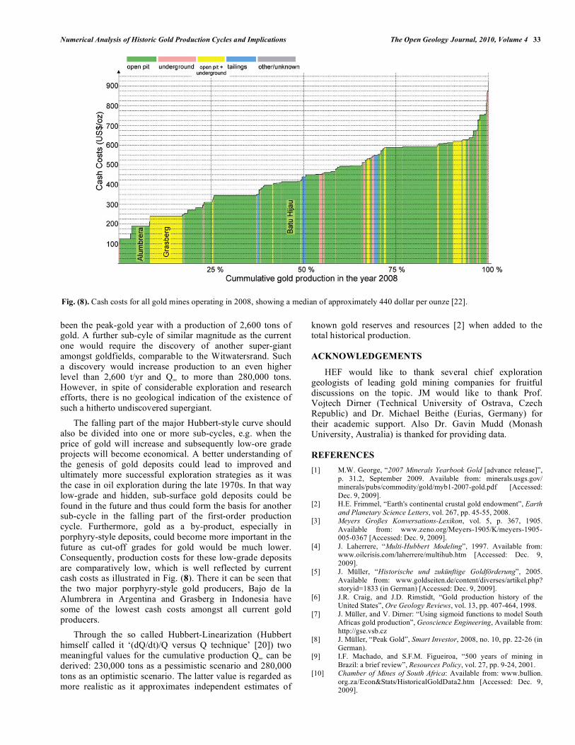
The falling part of the major Hubbert-style curve should also be divided into one or more sub-cycles, e.g. when the price of gold will increase and subsequently low-ore grade projects will become economical. A better understanding of the genesis of gold deposits could lead to improved and ultimately more successful exploration strategies as it was the case in oil exploration during the late 1970s. In that way low-grade and hidden, sub-surface gold deposits could be found in the future and thus could form the basis for another sub-cycle in the falling part of the first-order production cycle. Furthermore, gold as a by-product, especially in porphyry-style deposits, could become more important in the future as cut-off grades for gold would be much lower. Consequently, production costs for these low-grade deposits are comparatively low, which is well reflected by current cash costs as illustrated in Fig. (8). There it can be seen that the two major porphyry-style gold producers, Bajo de la Alumbrera in Argentina and Grasberg in Indonesia have some of the lowest cash costs amongst all current gold producers.

Through the so called Hubbert-Linearization (Hubbert himself called it ‘(dQ/dt)/Q versus Q technique’ [20]) two meaningful values for the cumulative production Q can be derived: 230,000 tons as a pessimistic scenario and 280,000 tons as an optimistic scenario. The latter value is regarded as more realistic as it approximates independent estimates of

known gold reserves and resources [2] when added to the total historical production.

ACKNOWLEDGEMENTS

HEF would like to thank several chief exploration geologists of leading gold mining companies for fruitful discussions on the topic. JM would like to thank Prof. Vojtech Dirner (Technical University of Ostrava, Czech Republic) and Dr. Michael Beithe (Eurias, Germany) for their academic support. Also Dr. Gavin Mudd (Monash University, Australia) is thanked for providing data.

REFERENCES

[1] M.W. George, “2007 Minerals Yearbook Gold [advance release]”, p. 31.2, September 2009. Available from: minerals.usgs.gov/ minerals/pubs/commodity/gold/myb1-2007-gold.pdf [Accessed: Dec. 9, 2009].

[2] H.E. Frimmel, “Earth's continental crustal gold endowment”, Earth

and Planetary Science Letters, vol. 267, pp. 45-55, 2008. [3] Meyers Großes Konversations-Lexikon, vol. 5, p. 367, 1905.

Available from: www.zeno.org/Meyers-1905/K/meyers-1905-005-0367 [Accessed: Dec. 9, 2009].

[4] J. Laherrere, “Multi-Hubbert Modeling”, 1997. Available from: www.oilcrisis.com/laherrere/multihub.htm [Accessed: Dec. 9, 2009].

[5] J. Müller, “Historische und zukünftige Goldförderung”, 2005. Available from: www.goldseiten.de/content/diverses/artikel.php? storyid=1833 (in German) [Accessed: Dec. 9, 2009].

[6] J.R. Craig, and J.D. Rimstidt, “Gold production history of the United States”, Ore Geology Reviews, vol. 13, pp. 407-464, 1998.

[7] J. Müller, and V. Dirner: “Using sigmoid functions to model South Africas gold production”, Geoscience Engineering, Available from: http://gse.vsb.cz

[8] J. Müller, “Peak Gold”, Smart Investor, 2008, no. 10, pp. 22-26 (in German).

[9] I.F. Machado, and S.F.M. Figueiroa, “500 years of mining in Brazil: a brief review”, Resources Policy, vol. 27, pp. 9-24, 2001.

[10] Chamber of Mines of South Africa: Available from: www.bullion. org.za/Econ&Stats/HistoricalGoldData2.htm [Accessed: Dec. 9, 2009].

Fig. (8). Cash costs for all gold mines operating in 2008, showing a median of approximately 440 dollar per ounze [22].

34 The Open Geology Journal, 2010, Volume 4 Müller and Frimmel

[11] Natural Resources Canada: Available from: www.nrcan-rncan.gc. ca [Accessed: Dec. 9, 2009].

[12] G.M. Mudd, “Global trends in gold mining: Towards quantifying environmental and resource sustainability?”, Resources Policy, vol. 32, pp. 42-56, 2007.

[13] D. Meadows, D. Meadows, and J. Randers, Die neuen Grenzen des Wachstums. Stuttgart: Deutsche Verlags-Anstalt, 1992, p. 149, (in German).

[14] British Petrol, Statistical review of world energy 2009. Available from: www.bp.com/statisticalreview/ [Accessed: Dec. 9, 2009].

[15] V.E. McKelvey, “Mineral resource estimates and public policy”, American Scientist, vol. 60, no. 1, pp. 32-40, 1972.

[16] T. McKeith, “Exploration: A gold industry perspective”, World

Mining Investment Congress, London, June 2009. Available from: http://www.goldfields.co.za/presentations/2009/world–mining–cong ress_09.pdf [Accessed: Dec. 9, 2009].

[17] M.W. George, “USGS Gold statistics and information 2009”, Available from: minerals.usgs.gov/minerals/pubs/commodity/gold/ mcs-2009-gold.pdf [Accessed: Dec. 9, 2009].

[18] C.J.H. Hartnady, “South Africa’s gold production and reserves”, South African Journal of Science, vol. 105, p. 328, 2009.

[19] GFMS Ltd. Available from: www.research.gold.org/supply–

demand/ [Accessed: Dec. 9, 2009]. [20] M.K. Hubbert, “Techniques of prediction as applied to production

of oil and gas”, NBS Special Publication 631, May 1982. Available from: http://rutledge.caltech.edu/King%20Hubbert%20Techniques %20of%20Prediction%20as%20applied%20to%20the%20production%20of%20oil%20and%20gas.pdf [Accessed: Dec. 9, 2009].

[21] M.K. Hubbert: “Nuclear energy and the fossil fuels”, Spring

Meeting American Petroleum Institute, San Antonio 1956, publication no. 95. Available from: www.hubbertpeak.com/ Hubbert/1956/1956.pdf [Accessed: Dec. 9, 2009].

[22] Raw Materials Group: Raw Materials Data Base, Version 2009 11.30. Solna, Sweden, Available at: www.rmg.se

Received: December 14, 2009 Revised: January 20, 2010 Accepted: January 22, 2010

© Müller and Frimmel; Licensee Bentham Open.

This is an open access article licensed under the terms of the Creative Commons Attribution Non-Commercial License (http: //creativecommons.org/licenses/by-nc/ 3.0/) which permits unrestricted, non-commercial use, distribution and reproduction in any medium, provided the work is properly cited.