ONTROL OPTIM c

Copyright © by SIAM. Unauthorized reproduction of this article is prohibited.

SIAM J. CONTROL OPTIM. c© 2008 Society for Industrial and Applied MathematicsVol. 47, No. 2, pp. 553–574

CONTROL OF A TIP-FORCE DESTABILIZED SHEAR BEAMBY OBSERVER-BASED BOUNDARY FEEDBACK∗

MIROSLAV KRSTIC† , BAO-ZHU GUO‡ , ANDRAS BALOGH§ , AND

ANDREY SMYSHLYAEV¶

Abstract. We consider a model of the undamped shear beam with a destabilizing boundarycondition. The motivation for this model comes from atomic force microscopy, where the tip of thecantilever beam is destabilized by van der Waals forces acting between the tip and the materialsurface. Previous research efforts relied on collocated actuation and sensing at the tip, exploiting thepassivity property between the corresponding input and output in the beam model. In this paper wedesign a stabilizing output-feedback controller in a noncollocated setting, with measurements at thefree end (tip) of the beam and actuation at the beam base. Our control design is a novel combinationof the classical “damping boundary feedback” idea with a recently developed backstepping approach.A change of variables is constructed which converts the beam model into a wave equation (for a veryshort string) with boundary damping. This approach is physically intuitive and allows both an elegantstability analysis and an easy selection of design parameters for achieving desired performance. Ourobserver design is a dual of the similar ideas, combining the damping feedback with backstepping,adapted to the observer error system. Both stability and well-posedness of the closed-loop systemare proved. The simulation results are presented.

Key words. distributed parameter systems, shear beam, backstepping, stabilization, boundarycontrol

AMS subject classifications. 35J05, 93B07, 93D15, 93B52, 93B60

DOI. 10.1137/060676969

1. Introduction. Flexible beams constitute an important benchmark problemin many application areas ranging from aerospace to civil structures. In some of theexciting modern fields such as atomic force microscopy, the cantilever beam is morethan just a prototype problem and constitutes an important application topic in itsown right.

In this paper we consider a model of the undamped shear beam [3] with a destabi-lizing boundary condition. It consists of a wave equation coupled with a second-order-in-space ODE or can be alternatively represented as a fourth-order-in-space/second-order-in-time PDE. This makes it more complex than the Euler–Bernoulli model [3],similar in structure to the Rayleigh beam model [3], and slightly simpler than the Tim-oshenko model [3]. The destabilizing boundary condition is motivated by the physicsof the atomic force microscopy (AFM), where the tip of the cantilever beam is desta-bilized by van der Waals forces acting between the tip and the material surface [19].

∗Received by the editors December 7, 2006; accepted for publication (in revised form) July 1,2007; published electronically February 6, 2008. This work was supported by the National ScienceFoundation and by the Los Alamos National Laboratory.

http://www.siam.org/journals/sicon/47-2/67696.html†Corresponding author. Department of Mechanical and Aerospace Engineering, University of

California at San Diego, La Jolla, CA 92093 ([email protected]).‡Academy of Mathematics and Systems Science, Academia Sinica, Beijing 100080, People’s

Republic of China, and School of Computational and Applied Mathematics, University of theWitwatersrand, Wits 2050, Johannesburg, South Africa ([email protected]).

§Department of Mathematics, University of Texas – Pan American, Edinburg, TX 78541([email protected]).

¶Department of Mechanical and Aerospace Engineering, University of California at San Diego,La Jolla, CA 92093 ([email protected]).

553


554 M. KRSTIC, B.-Z. GUO, A. BALOGH, AND A. SMYSHLYAEV

Extensive literature exists on control of beam models [1, 2, 8, 4, 7, 9, 11, 17, 20, 21].However, previous research efforts all relied on collocated actuation and sensing atthe tip, exploiting in an elegant way the passivity property between the correspondinginput and output in the beam model. The main drawback of this approach is thatthe tip of the beam is not a very convenient place to put an actuator. Therefore suchfeedbacks are usually implemented via passive dampers or through rather elaborateways, such as electromagnets or small airjets at the tip of the beam.

Our objective is different—to design controllers implementable through noncollo-cated architecture, with actuation only at the base and sensing only at the tip of thebeam. This architecture makes active control more readily implementable to severalapplications; for example, in AFM this allows a natural use of piezo actuation at thebase of the beam. Our control design is a novel combination of the classical “damp-ing boundary feedback” idea with a recently developed backstepping approach, whichhas been used to design boundary controllers [12, 14] and observers [13] for parabolicequations and for the Timoshenko beam model with a small amount of Kelvin–Voigtdamping [6]. A change of variables is constructed which converts the beam model intoa wave equation (for a very short string) with boundary damping. This approach isphysically intuitive and allows both an elegant stability analysis and an easy selectionof design parameters for achieving desired performance. Our observer design is a dualof the similar ideas, combining the damping feedback with backstepping, adapted tothe observer error system.

In addition to rigorous stability and well-posedness analysis of the closed-loopsystem, we also present the results of simulations that illustrate the performance ofthe controller.

2. Model. The shear beam model can be represented in a number of equivalentways [3]. One often used form is a single second-order-in-time fourth-order-in-spacePDE

(2.1) awtt(x, t) − δwxxtt(x, t) + wxxxx(x, t) = 0, 0 < x < 1, t > 0,

with a, δ > 0 and two “free end” boundary conditions δwtt(0, t) = wxx(0, t) andδwxtt(0, t) = wxxx(0, t) − q a

δw(0, t).We, however, will use another common form of this model, consisting of a wave

equation coupled with a second-order ODE:

(2.2)

⎧⎪⎪⎪⎪⎪⎪⎪⎪⎪⎪⎪⎨⎪⎪⎪⎪⎪⎪⎪⎪⎪⎪⎪⎩

δwtt(x, t) = wxx(x, t) − αx(x, t), 0 < x < 1, t > 0,

wx(0, t) = α(0, t) − qw(0, t), t ≥ 0,

w(1, t) = u1(t), t ≥ 0,

0 = αxx(x, t) − b2α(x, t) + b2wx(x, t), 0 < x < 1, t > 0,

αx(0, t) = 0, t ≥ 0,

α(1, t) = u2(t), t ≥ 0,

y(t) = (w(0, t), α(0, t)), t ≥ 0,

which is obtained from (2.1) by introducing a new state αx = wxx−δwtt and denotingb =

√a/δ. The state w represents the transversal displacement of the beam, and α is

the angle due to bending. The objective is to use the control input u(t) = (u1(t), u2(t))at the base of the beam to stabilize the tip of the beam with the measurement y(t)available only at the free end.


CONTROL OF A TIP-FORCE DESTABILIZED SHEAR BEAM 555

It is important to note the term −qw(0, t) in the boundary condition (2.2). Thistype of boundary condition corresponds to situations where the tip of the beam issubject to an external force which depends on the displacement. Such a force arises inAFM as a van der Waals force acting between the atoms on the material surface andthe beam tip. The term −qw(0, t) is the linearized model of that force; the originalnonlinear model has cubic nonlinearity [19]. Typically q > 0 has a destabilizing effect(in that case, one can think of this parameter as “antistiffness”), whereas q < 0 hasa stabilizing effect. We stress that this force occurs on the opposite end of the beamfrom where the actuator is located. If the actuator were at the tip, canceling the effectof this force would be trivial. In the configuration that we pursue here, stabilization,and even vibration suppression when q = 0, is a nontrivial problem.

We will first present control and observer designs separately to make the ideasclear and then prove the certainty equivalence principle and well-posedness of theclosed-loop system in sections 5–7.

3. Controller. In order to proceed with the control design we first need to writethe model (2.2) in yet another form. To this end, we solve the ODE part of (2.2) asa two point boundary value problem for α with boundary condition αx(0, t) = 0:

(3.1) α(x, t) = cosh(bx)α(0, t) − b

∫ x

0

sinh(b(x− s))wx(s, t) ds.

Setting x = 1 in (3.1) and using the boundary condition α(1, t) = u2(t), we canexpress α(0, t) in terms of w and u2:

(3.2) α(0, t) =1

cosh(b)u2(t) +

b

cosh(b)

∫ 1

0

sinh(b(1 − s))wx(s, t) ds.

Next, we differentiate (3.1) in x and substitute the result into the first equationof (2.2). This way, instead of a wave equation coupled with a second-order ODE, weobtain a single hyperbolic partial integrodifferential equation for w:

(3.3)

⎧⎪⎪⎪⎪⎪⎪⎪⎪⎪⎪⎪⎪⎨⎪⎪⎪⎪⎪⎪⎪⎪⎪⎪⎪⎪⎩

δwtt(x, t) = wxx(x, t) − b2 cosh(bx)w(0, t) + b3∫ x

0

sinh(b(x− y))w(y, t)dy

+ b2w(x, t) − b sinh(bx)

cosh(b)

[u2(t) + b

∫ 1

0

sinh(b(1 − s))wx(s, t) ds

],

wx(0, t) =1

cosh(b)

[u2(t) + b

∫ 1

0

sinh(b(1 − s))wx(s, t) ds

]− qw(0, t),

w(1, t) = u1(t).

Since the backstepping control design [12] needs the PDE to be in a “strict-feedback”form (in other words, its right-hand side must be “causal” in x), we are going touse the control u2(t) to cancel the definite integral both in the domain and in theboundary condition:

(3.4) u2(t) = −b

∫ 1

0

sinh(b(1 − s))wx(s, t) ds.



We get the following PDE:

(3.5)

⎧⎪⎪⎪⎪⎪⎨⎪⎪⎪⎪⎪⎩

δwtt(x, t) = wxx(x, t) + b2w(x, t) − b2 cosh(bx)w(0, t)

+ b3∫ x

0

sinh(b(x− y))w(y, t)dy,

wx(0, t) = −qw(0, t),

w(1, t) = u1(t) .

The basic idea of the backstepping design is to use the transformation

(3.6) w(x, t) = w(x, t) −∫ x

0

k(x, y)w(y, t) dy ,

with specially designed control kernel k(x, y) along with the boundary feedback law

(3.7)

⎧⎪⎪⎪⎨⎪⎪⎪⎩

u1(t) = w(1, t),

wx(1, t) = k(1, 1)w(1, t) − c1wt(1, t)

+ c1

∫ 1

0

k(1, y)wt(y, t) dy +

∫ 1

0

kx(1, y)w(y, t) dy

to map (3.5) into the exponentially stable target system

(3.8)

⎧⎪⎨⎪⎩

δwtt(x, t) = wxx(x, t),

wx(0, t) = c0w(0, t),

wx(1, t) = −c1wt(1, t),

where c0 > 0 and c1 > 0 are design parameters. The system (3.8) is exponentiallystable at the origin iff c0 and c1 are positive. Note the crucial difference betweenthe second equations of (3.5) and (3.8)—the destabilizing negative sign in the formerand the stabilizing positive sign in the latter. The gain kernel k(x, y) is given by thefollowing PDE:

(3.9)

⎧⎪⎪⎪⎪⎪⎪⎪⎪⎪⎪⎨⎪⎪⎪⎪⎪⎪⎪⎪⎪⎪⎩

kxx(x, y) = kyy(x, y) + b2k(x, y) − b3 sinh(b(x− y))

+ b3∫ x

y

k(x, ξ) sinh(b(ξ − y))dξ,

k(x, x) = −b2

2x− c0 − q,

ky(x, 0) = −b2[cosh(bx) −

∫ x

0

k(x, y) cosh(by)dy

]− qk(x, 0),

which is obtained by substituting (3.6) into (3.8) and matching the terms. Incidentally,this equation for k(x, y) is in the same class as the one obtained in the control design forparabolic PDEs [12]. As shown in [12], the PDE (3.9) has a unique solution k ∈ C2(Ω).



It can be solved either numerically or by using the following symbolic recursion:

(3.10)

⎧⎪⎪⎪⎪⎪⎪⎪⎪⎪⎪⎪⎪⎪⎪⎪⎪⎪⎪⎪⎪⎪⎪⎨⎪⎪⎪⎪⎪⎪⎪⎪⎪⎪⎪⎪⎪⎪⎪⎪⎪⎪⎪⎪⎪⎪⎩

k(x, y) = limn→∞

kn(x, y),

k0 = − b

2[− sinh(b(x− y)) + by cosh(b(x− y))] − c0 − q,

kn+1 = k0 + b2∫ x+y

2

x−y2

∫ x−y2

0

kn(σ + s, σ − s)dsdσ + q

∫ x−y

0

kn(σ, 0)dσ

+ b2∫ x−y

2

0

∫ σ

0

[2kn(σ + s, σ − s) − kn(σ, s) cosh(bs)]dsdσ

+ b3∫ x+y

2

x−y2

∫ x−y2

0

∫ σ+s

σ−s

kn(σ + s, ξ) sinh(b(ξ − σ + s))dξdsdσ

+ 2b3∫ x−y

2

0

∫ σ

0

∫ σ+s

σ−s

kn(σ + s, ξ) sinh(b(ξ − σ + s))dξdsdσ.

The first step of this recursion provides approximate control gain kernels, which areexplicit:

(3.11)

⎧⎪⎪⎪⎪⎪⎨⎪⎪⎪⎪⎪⎩

k0(1, y) = − b

2[− sinh(b(1 − y)) + by cosh(b(1 − y))] − c0 − q,

k0x(1, y) = − b

2[− cosh(b(1 − y)) + by sinh(b(1 − y))],

k0(1, 1) = k(1, 1) = −b2

2− c0 − q.

Since k ∈ C2(Ω), the transformation (3.6) is bounded invertible, and therefore thesystem (3.5) with the controller (3.7) dynamically behaves as (3.8). The importantquestion is why we chose our system’s “target” behavior as in (3.8). This PDE with ahomogeneous Dirichlet boundary condition at x = 0 (i.e., for c0 = ∞) has been studiedin many papers on control of wave equations by “boundary damper” feedback. Fora large positive c0, our “target” system has a similar behavior to those well-studiedproblems. Obviously, the most desirable behavior would be with c0 = 0; however,such behavior is achievable only if one could put an actuator at the tip. In thatcase, the end x = 0 would be clamped, and the end x = 1 would be actuated with a“boundary damper.” Since we are pursuing the opposite problem, where the tip endx = 0 is free and the actuator is at the opposite end x = 1, it is only through thevery sophisticated construction that we presented above that a behavior similar tothe boundary damper feedback is achievable. The plant boundary condition at x = 0is of Robin type, and no state transformation can change it into Dirichlet. However,we can change it into a Robin condition of favorable sign (c0 > 0) and make it behavesimilar to a Dirichlet condition (with large c0). To achieve all of this, we constructthe change of variable (3.6) which starts at x = 0 and goes towards x = 1, collectingall of the terms in the shear beam model and converting them into a wave equationmodel. But it is ultimately the boundary feedback (3.7) that absorbs the effects of thetransformation and results in a damping boundary condition at the end x = 1. Clearlysuch feedback has to be rather complicated because it achieves a similar effect as theboundary damper but from the opposite end. In addition to the first two terms onthe right-hand side of (3.7), which arise in boundary dampers and essentially amountto PD control, our feedback law incorporates the two integral operators acting on



the displacement and velocity fields (as we will show in the next section, the directmeasurement of w(x, t) and wt(x, t) along the whole beam is not necessary).

The control law (3.7) has to be implemented by solving for w(1, t). In the fre-quency domain it is equivalent to employing a low pass filter acting on wx(1, s) andthe integral operator:

(3.12) u1(s) =1

c1s + b2

2 + c0 + q

[−wx(1, s) +

∫ 1

0

(c1sk(1, y) + kx(1, y))w(y, s) dy

].

In AFM u1 is implemented via a piezo actuator which actuates the beam base dis-placement. Implementation of u2 would involve two piezo actuators to produce acommanded u2.

4. Observer. Before we start with the observer design, we write the model (3.3)in a slightly different form using (3.2):

(4.1)

⎧⎪⎪⎪⎪⎪⎪⎪⎨⎪⎪⎪⎪⎪⎪⎪⎩

δwtt(x, t) = wxx(x, t) + b2w(x, t) + b3∫ x

0


− b2 cosh(bx)w(0, t) − b sinh(bx)α(0, t),

wx(0, t) = α(0, t) − qw(0, t),

w(1, t) = u1(t).

Note that in this form u2 is not selected as in (3.4) and the observer is designed forarbitrary inputs u1 and u2.

We assume that the only available measurements are of the tip displacementw(0, t) and of the tip angle due to bending α(0, t). In AFM the displacement and theslope of the tip are routinely measured using a laser and a photodiode.

The observer is designed along the lines of the design presented in [13] for parabolicsystems and follows a standard finite-dimensional approach “copy of the plant plusoutput injection terms”:

(4.2)

⎧⎪⎪⎪⎪⎪⎪⎪⎪⎪⎪⎪⎨⎪⎪⎪⎪⎪⎪⎪⎪⎪⎪⎪⎩


0


− b2 cosh(bx)w(0, t) − b sinh(bx)α(0, t)

+ py(x, 0)[w(0, t) − w(0, t)] − c2p(x, 0)[wt(0, t) − wt(0, t)],

wx(0, t) = α(0, t) − qw(0, t) + p(0, 0)[w(0, t) − w(0, t)]

− c2[wt(0, t) − wt(0, t)],

w(1, t) = u1(t).

The constant c2 > 0 is the design parameter that sets the convergence rate of theobserver. Note that the output error terms are injected both in the domain and inthe boundary condition. The observer gains p(x, 0), py(x, 0), and p(0, 0) in (4.2) aredetermined by solving the following PDE in Ω = {(x, y)| 0 ≤ y ≤ x ≤ 1}:

(4.3)

⎧⎪⎪⎪⎪⎪⎪⎪⎨⎪⎪⎪⎪⎪⎪⎪⎩

pyy(x, y) = pxx(x, y) + b2p(x, y) − b3 sinh(b(x− y))

+ b3∫ x

y

p(ξ, y) sinh(b(x− ξ))dξ,

p(x, x) =b2

2(x− 1),

p(1, y) = 0.



It has been shown in [13] that this equation has a unique solution p ∈ C2(Ω). Onecan see the similarity between this PDE and the one for the control kernel. Thisis due to the duality between observer and control designs, a concept well known infinite-dimensional control. One can think of the gains p(x, 0), py(x, 0), and p(0, 0) asdual counterparts to the control gains k(1, y), kx(1, y), and k(1, 1).

(4.3) can be solved numerically or symbolically using the following recursive pro-cedure [13]:

(4.4)

⎧⎪⎪⎪⎪⎪⎪⎪⎪⎪⎪⎪⎪⎪⎪⎪⎪⎪⎪⎪⎪⎪⎪⎨⎪⎪⎪⎪⎪⎪⎪⎪⎪⎪⎪⎪⎪⎪⎪⎪⎪⎪⎪⎪⎪⎪⎩

p(x, y) = limn→∞

pn(x, y),

p0 = − b

2[− sinh(b(x− y)) + b(1 − x) cosh(b(x− y))],

pn+1 = p0 + b2∫ 2−x−y

2

x−y2

∫ x−y2

0

pn(σ + s, σ − s)dsdσ

+ 2b2∫ x−y

2

0

∫ σ

0

pn(σ + s, σ − s)dsdσ

+ b3∫ 2−x−y

2

x−y2

∫ x−y2

0

∫ σ+s

σ−s

pn(σ + s, ξ) sinh(b(ξ − σ + s))dξdsdσ

+ 2b3∫ x−y

2

0

∫ σ

0

∫ σ+s

σ−s

pn(σ + s, ξ) sinh(b(ξ − σ + s))dξdsdσ.

The observer gain in the boundary condition (4.2) is known exactly:

(4.5) p(0, 0) = −b2

2.

Let us denote the observer error by ε(x, t) = w(x, t) − w(x, t). Using (4.2) and(4.1) we obtain the observer error dynamics

(4.6)

⎧⎪⎪⎪⎪⎪⎪⎪⎨⎪⎪⎪⎪⎪⎪⎪⎩

δεtt(x, t) = εxx(x, t) + b2ε(x, t) + b3∫ x

0

sinh(b(x− y))ε(y, t)dy

− py(x, 0)ε(0, t) + c2p(x, 0)εt(0, t),

εx(0, t) = −p(0, 0)ε(0, t) + c2εt(0, t),

ε(1, t) = 0.

The convergence of the observer is established by the following lemma.Lemma 4.1. Suppose the classical solution of (4.6) exists. Then the invertible

transformation

(4.7)

⎧⎪⎪⎨⎪⎪⎩

ε(x, t) = ε(x, t) −∫ x

0

p(x, y)ε(y, t)dy = [(I − P1)ε](x, t),

ε(x, t) = [(I − P1)−1ε](x, t) = ε(x, t) −

∫ x

0

p�(x, y)ε(y, t)dy

converts the error system (4.6) into the exponentially stable system

(4.8)

⎧⎪⎨⎪⎩

δεtt(x, t) = εxx(x, t),

εx(0, t) = c2εt(0, t),

ε(1, t) = 0.



Proof. We differentiate the transformation (4.7) with respect to t and x:

δεtt(x, t) = δεtt(x, t) −∫ x

0

p(x, y)δεtt(y, t)dy − εxx(x, t) + εxx(x, t)

= δεtt(x, t) −∫ x

0

pyy(x, y)ε(y, t)dy − p(x, x)εx(x, t) + p(x, 0)εx(0, t)

+ py(x, x)ε(x, t) − py(x, 0)ε(0, t) − εxx(x, t) + [2px(x, x) + py(x, x)]ε(x, t)

+ p(x, x)εx(x, t) +

∫ x

0

pxx(x, y)ε(y, t) dy + εxx(x, t)

= εxx(x, t) + b2ε(x, t) + c2p(x, 0)εt(0, t) − py(x, 0)ε(0, t)

+

∫ x

0

(pxx(x, y) − pyy(x, y) + b2p(x, y))ε(y, t) dy.

Using the observer gain PDE (4.3) in the above equation we get the governing equationof (4.8).

Next we differentiate the transformation (4.7) with respect to x and set x = 0:

εx(0, t) = εx(0) − p(0, 0)ε(0, t) .

Comparing this with the boundary condition of (4.6), which can be written as

εx(0, t) = −p(0, 0)ε(0, t) + c2εt(0, t),

we get the boundary condition of (4.8) at x = 0. Finally, the boundary condition atx = 1 is obviously satisfied because p(1, y) = 0.

5. Output feedback. Consider the observer (4.2) and the control (3.4), (3.7)with the observer state instead of the unmeasured plant state:

(5.1)

⎧⎪⎪⎪⎪⎪⎪⎪⎪⎨⎪⎪⎪⎪⎪⎪⎪⎪⎩

u1(t) = w(1, t),

wx(1, t) = k(1, 1)w(1, t) − c1wt(1, t)

+ c1

∫ 1

0

k(1, y)wt(y, t)dy +

∫ 1

0

kx(1, y)w(y, t)dy,

u2(t) = −b

∫ 1

0

sinh(b(1 − y))wx(y, t) dy.

We employ an invertible state transformation

(5.2)

⎧⎪⎪⎨⎪⎪⎩

w(x, t) = w(x, t) −∫ x

0

k(x, y)w(y, t)dy = [(I − P2)w](x, y),

w(x, t) = [(I − P2)−1w](x, y) = w(x, t) −

∫ x

0

k�(x, y)w(x, y)dy,

where k(x, y) is given by (3.10) and both k(x, y) and k�(x, y) are of C2 in Ω [12].



Lemma 5.1. Suppose the classical solution of (4.2) with the control (5.1) exists.Then the transformation (5.2) converts (4.2) and (5.1) into

(5.3)

⎧⎪⎪⎪⎪⎪⎪⎪⎪⎪⎪⎪⎪⎨⎪⎪⎪⎪⎪⎪⎪⎪⎪⎪⎪⎪⎩

δwtt(x, t) = wxx(x, t) − b sinh(bx)α(0, t) + k(x, 0)α(0, t) + py(x, 0)ε(0, t)

+ k(x, 0)p(0, 0)ε(0, t) + ky(x, 0)ε(0, t) − c2k(x, 0)εt(0, t)

+ b

∫ x

0

k(x, y) sinh(by)dy α(0, t) −∫ x

0

k(x, y)py(y, 0)dy ε(0, t)

− c2p(x, 0)εt(0, t) + c2

∫ x

0

k(x, y)p(y, 0)dy εt(0, t),

wx(0, t) = c0w(0, t) + α(0, t) + p(0, 0)ε(0, t) − c2εt(0, t),

wx(1, t) = −c1wt(1, t).

Proof. First we compute the second spatial derivative of the transformation (5.2):

wxx(x, t) = wxx(x, t) − [2kx(x, x) + ky(x, x)]w(x, t) − k(x, x)wx(x, t)

−∫ x

0

kxx(x, y)w(y, t)dy.(5.4)

The next step is to compute wtt:

(5.5)

δwtt(x, t) = δwtt(x, t) −∫ x

0

k(x, y)δwtt(y, t)dy

= wxx(x, t) + b2w(x, t) + b3∫ x

0


− b2 cosh(bx)w(0, t) − b sinh(bx)α(0, t) + py(x, 0)ε(0, t)

− c2p(x, 0)εt(0, t) −∫ x

0

k(x, y)wyy(y, t)dy − b2∫ x

0

k(x, y)w(y, t)dy

− b3∫ x

0

∫ x

y

k(x, ξ) sinh(b(ξ − y))w(y, t)dy

+ b2∫ x

0

k(x, y) cosh(by)dyw(0, t) + b

∫ x

0

k(x, y) sinh(by)dy α(0, t)

−∫ x

0

k(x, y)py(y, 0)dyε(0, t) + c2

∫ x

0

k(x, y)p(y, 0)dyεt(0, t).

We notice that

∫ x

0

k(x, y)wyy(y, t)dy =

∫ x

0

kyy(x, y)w(y, t)dy

+ k(x, x)wx(x, t) − k(x, 0)wx(0, t)

− ky(x, x)w(x, t) + ky(x, 0)w(0, t)

=

∫ x

0

kyy(x, y)w(y, t)dy + k(x, x)wx(x, t) − k(x, 0)α(0, t)

+ qk(x, 0)w(0, t) + k(x, 0)p(0, 0)ε(0, t) + c2k(x, 0)εt(0, t)

− ky(x, x)w(x, t) − ky(x, 0)ε(0, t) + ky(x, 0)w(0, t).

(5.6)

Substracting (5.4) from (5.5) and using (5.6), we get (5.3).



The boundary condition at x = 1 is verified in the following way:

0 = wx(1, t) + c1wt(1, t)

= wx(1, t) − k(1, 1)w(1, t) −∫ 1

0

kx(1, y)w(y, t)

+ c1wt(1, t) − c1

∫ 1

0

k(1, y)wt(y, t)dy,

which gives exactly the controller (5.1). Finally, for the boundary condition at x = 0we have

wx(0, t) = wx(0, t) − k(0, 0)w(0, t) = wx(0, t) − k(0, 0)w(0, t)

= α(0, t) − qw(0, t) + p(0, 0)ε(0, t) − c2εt(0, t) − k(0, 0)w(0, t)

= c0w(0, t) + α(0, t) + p(0, 0)ε(0, t) − c2εt(0, t).

The proof is complete.

6. Well-posedness and stability of the transformed system. Lemmas 4.1and 5.1 establish the following transformed system (ε, w) which is a cascade of twowave equations (with additional integral terms):

(6.1)

⎧⎪⎪⎪⎪⎪⎪⎪⎪⎪⎪⎪⎪⎪⎪⎪⎪⎪⎪⎪⎪⎨⎪⎪⎪⎪⎪⎪⎪⎪⎪⎪⎪⎪⎪⎪⎪⎪⎪⎪⎪⎪⎩

δεtt(x, t) = εxx(x, t),

εx(0, t) = c2εt(0, t),

ε(1, t) = 0,

δwtt(x, t) = wxx(x, t) − b sinh(bx)α(0, t) + k(x, 0)α(0, t) − c2k(x, 0)εt(0, t)

+ py(x, 0)ε(0, t) + k(x, 0)p(0, 0)ε(0, t) + ky(x, 0)ε(0, t)

+ b

∫ x

0

k(x, y) sinh(by) dyα(0, t) −∫ x

0

k(x, y)py(y, 0) dyε(0, t)

− c2p(x, 0)εt(0, t) + c2

∫ x

0

k(x, y)p(y, 0)dyεt(0, t),

wx(0, t) = c0w(0, t) + α(0, t) + p(0, 0)εt(0, t) − c2εt(0, t),

wx(1, t) = −c1wt(1, t).

Here α(0, t) is expressed in terms of ε using (3.2) and (4.7):

α(0, t) =b

cosh(b)

∫ 1

0

sinh(b(1 − x))[εx(x, t) − p(x, x)ε(x, t)] dx

− b

cosh(b)

∫ 1

0

∫ 1

x

sinh(b(1 − y))px(y, x) dy ε(x, t) dx.(6.2)

From (6.2) and the fact that ε(1, t) = 0, we know that there exists a constantC1 > 0 such that

(6.3) |α(0, t)|2 ≤ C1

∫ 1

0

ε2x(x, t) dx.

We consider the system (6.1) in the space H = H1R(0, 1)×L2(0, 1)×H1(0, 1)×L2(0, 1),



H1R(0, 1) = {f | f ∈ H1(0, 1)| f(1) = 0}, with the inner product

〈(f1, g1, φ1, ψ1), (f2, g2, φ2, ψ2)〉

= K

∫ 1

0

[f ′1(x)f ′

2(x) +1

δg1(x)g2(x) + δ0(x− 1)(f ′

1(x)g2(x) + g1(x)f ′2(x))

]dx

+

∫ 1

0

[φ′

1(x)φ′2(x) +

1

δψ1(x)ψ2(x) + δ0(x + 1)(φ′

1(x)ψ2(x) + ψ1(x)φ′2(x))

]dx

+ c1φ1(0)φ2(0) ∀ (f, g, φ, ψ) ∈ H,

where δ0 > 0 is sufficiently small so that above inner product is well-defined andK > 0 is large enough so that A is dissipative in H as in the proof of Lemma 5.1below. Define the system operator A : D(A)(⊂ H) → H as follows:

(6.4)

⎧⎪⎪⎪⎪⎪⎪⎪⎪⎪⎪⎪⎪⎪⎪⎪⎪⎪⎪⎪⎪⎪⎪⎪⎪⎪⎪⎪⎪⎪⎪⎪⎪⎪⎪⎪⎪⎪⎪⎨⎪⎪⎪⎪⎪⎪⎪⎪⎪⎪⎪⎪⎪⎪⎪⎪⎪⎪⎪⎪⎪⎪⎪⎪⎪⎪⎪⎪⎪⎪⎪⎪⎪⎪⎪⎪⎪⎪⎩

D(A) =

{(f, g, φ, ψ) ∈ (H2(0, 1) ∩H1

R(0, 1)) ×H1R(0, 1) ×H2(0, 1)

× H1(0, 1)| f ′(0) =c2δg(0), φ′(1) = −c1

δψ(1)

φ′(0) = c0φ(0) +1

δ[p(0, 0) − c2]g(0) + α(0)

},

A(f, g, φ, ψ) =

(g

δ, f ′′,

ψ

δ, φ′′ − b sinh(bx)α(0) + [py(x, 0) + ky(x, 0)]f(0)

+ k(x, 0)[α(0) + p(0, 0)f(0)] −∫ x

0

k(x, y)py(y, 0)dyf(0)

+ b

∫ x

0

k(x, y) sinh(by)dy α(0) − c2δk(x, 0)g(0)

+c2δ

[−p(x, 0) +

∫ x

0

k(x, y)p(y, 0)dy

]g(0)

),

α(0) =b

cosh(b)

∫ 1

0

sinh(b(1 − x))[f ′(x) − p(x, x)f(x)] dx

− b

cosh(b)

∫ 1

0

∫ 1

x

sinh(b(1 − y))px(y, x) dyf(x) dx

∀ (f, g, φ, ψ) ∈ D(A).

Then the system (6.1) can be written as

(6.5)d

dt(ε(·, t), δεt(·, t), w(·, t), δwt(·, t)) = A(ε(·, t), δεt(·, t), w(·, t), δwt(·, t)).

Theorem 6.1. Let A be defined by (6.4). Then A generates an exponential stableC0-semigroup on H. For any initial value (ε(·, 0), δεt(·, 0), w(·, 0), δwt(·, 0)) ∈ H,there exists a unique (mild) solution to (6.1) such that (ε(·, t), δεt(·, t), w(·, t), δwt(·, t))∈ C([0,∞);H), and there exists a positive constant ω such that

‖(ε(·, t), δεt(·, t), w(·, t), δwt(·, t))‖H≤ e−ωt‖(ε(·, 0), δεt(·, 0), w(·, 0), δwt(·, 0))‖H .(6.6)

Moreover, if (ε(·, 0), δεt(·, 0), w(·, 0), δwt(·, 0)) ∈ D(A), then

(6.7) (ε(·, t), δεt(·, t), w(·, t), δwt(·, t)) ∈ C1([0,∞);H)

is the classical solution of (6.1).



Proof. Define the Lyapunov functions

(6.8) Eε(t) =1

2

∫ 1

0

[ε2x(x, t) + δε2

t (x, t)]dx + δ0

∫ 1

0

(x− 1)εx(x, t)δεt(x, t)dx

and

Ew(t) =1

2

∫ 1

0

[w2x(x, t) + δw2

t (x, t)]dx +δ02w2(0, t)

+ δ0

∫ 1

0

(1 + x)wx(x, t)δwt(x, t)dx.(6.9)

Both of them are positive definite for small δ0, δ0 > 0. The time derivatives of Eε andEw along the trajectory of (6.1) are, respectively,

(6.10) Eε(t) = −[c2 −

δ02

(1 + c22)

]ε2t (0, t) −

δ02

∫ 1

0

[ε2x(x, t) + δε2

t (x, t)]dx,

(6.11)

Ew(t) = −c1w2t (1, t) − c0w

2(0, t) − α(0, t)wt(0, t) − p(0, 0)wt(0, t)εt(0, t)

+ c2wt(0, t)εt(0, t) +

∫ 1

0

[k(x, 0) − b sinh(bx)]wt(x, t)dxα(0, t)

+

∫ 1

0

wt(x, t)py(x, 0)dx ε(0, t) + b

∫ 1

0

wt(x, t)dx

∫ x

0


+

∫ 1

0

wt(x, t)k(x, 0)dx p(0, 0)ε(0, t) +

∫ 1

0

wt(x, t)ky(x, 0)dx ε(0, t)

−∫ 1

0

wt(x, t)dx

∫ x

0

k(x, y)py(y, 0)dy ε(0, t) − c2

∫ 1

0

wt(x, t)k(x, 0)dx εt(0, t)

− c2

∫ 1

0

wt(x, t)p(x, 0)dx εt(0, t) + c2

∫ 1

0

wt(x, t)dx

∫ x

0

k(x, y)p(y, 0)dy εt(0, t)

− δ02

∫ 1

0

[w2x(x, t) + δw2

t (x, t)]dx− δδ02

w2t (0, t) + δ0(δ + c21)w

2t (1, t)

− δ02

[c0w(0, t) + α(0, t) + p(0, 0)εt(0, t) − c2εt(0, t)]2

+ δ0

∫ 1

0

(1 + x)wx(x, t)(k(x, 0) − b sinh(bx))dxα(0, t)

+ δ0

∫ 1

0

(1 + x)wx(x, t)(py(x, 0) + ky(x, 0) + p(0, 0)k(x, 0))dx ε(0, t)

+ bδ0

∫ 1

0

(1 + x)wx(x, t)dx

∫ x

0


− δ0

∫ 1

0

(1 + x)wx(x, t)dx

∫ x

0

k(x, y)py(y, 0)dy ε(0, t)

− c2δ0

∫ 1

0

(1 + x)wx(x, t)(p(x, 0) + k(x, 0))dx εt(0, t)

+ c2δ0

∫ 1

0

(1 + x)wx(x, t)dx

∫ x

0

k(x, y)p(y, 0)dy εt(0, t) + δ0w(0, t)wt(0, t).



Using (6.3) and the fact that k, p ∈ C2(Ω), we obtain

Ew(t) ≤[δ02

− δ1

] ∫ 1

0

[w2x(x, t) + δw2

t (x, t)]dx−[c0 +

δc202

− δ2

]w2(0, t)

−[c1 − δ0(δ + c21)

]w2

t (1, t) −[δδ02

− δ3

]w2

t (0, t)

+ C2α2(0, t) + C2ε

2(0, t) + C2ε2t (0, t),

where C2 and δi, i = 1, 2, 3, are some positive constants satisfying

(6.12) δ1 <δ02, δ2 < c0 +

δc202

, δ3 <δδ02

.

Now for large K > 0, we take the overall Laypunov function as

(6.13) E(t) = Ew(t) + KEε(t).

Since from (6.3), α2(0, t) + ε2(0, t) ≤ (1 +C1)‖ε2x(·, t)‖2

L2(0,1), we obtain its derivative

along the solution of (6.1) that

(6.14)

E(t) ≤ −K

[c2 −

δ02

(1 + c22)

]ε2t (0, t) −K

δ02

∫ 1

0

[ε2x(x, t) + δε2

t (x, t)]dx

−[δ02

− δ1

] ∫ 1

0

[w2x(x, t) + δw2

t (x, t)]dx−[c0 +

δc202

− δ2

]w2(0, t)

+ C2α2(0, t) + C2ε

2(0, t) + C2ε2t (0, t),

where we assumed that

(6.15) δ0(δ + c21) < c1.

Hence

(6.16)

E(t) ≤ −[K

(c2 −

δ02

(1 + c22)

)− C2

]ε2t (0, t)

−[K

δ02

− C2(1 + C1)

] ∫ 1

0

[ε2x(x, t) + δε2

t (x, t)]dx

−[δ02

− δ1

] ∫ 1

0

[w2x(x, t) + δw2

t (x, t)]dx−[c0 +

δc202

− δ2

]w2(0, t).

Choosing K > 0 sufficiently large, it follows from (6.16) that there exists an ω > 0such that

(6.17) E(t) ≤ −ωE(t).

The above procedure also gives the following estimate:

Re〈A(f, g, φ, ψ), (f, g, φ, ψ)〉H ≤ −ω‖(f, g, φ, ψ)‖2H ∀ (f, g, φ, ψ) ∈ D(A).

So A is dissipative in H ([10]), and if A generates a C0-semigroup, this semigroupmust be exponentially stable. By the Lumer–Phillips theorem (Theorem 4.3, p. 14 in[10]), the proof will be accomplished if we can show that A−1 exists and is boundedon H. Actually, a simple computation shows that

A−1(f, g, φ, ψ) = (f∗, g∗, φ∗, ψ∗) ∀ (f, g, φ, ψ) ∈ H,



where g∗ = δf, ψ∗ = δφ and

f∗(x) = c2f(0)(x− 1) +

∫ x

0

(x− τ)g(τ)dτ −∫ 1

0

(1 − τ)g(τ)dτ,

φ∗(x) =

∫ x

1

(x− τ)ψ(τ)dτ +

∫ x

1

(x− τ)F (τ)dτ − c1φ(1)x

−∫ 1

0

τψ(τ)dτ −∫ 1

0

τF (τ)dτ + φ∗(0),

φ∗(0) = − 1

c0

∫ 1

0

ψ(τ)dτ − 1

c0

∫ 1

0

F (τ)dτ − c1c0

φ(1) − α∗(0)

c0− p(0, 0) − c2

c0f(0),

F (x) = b sinh(bx)α∗(0) − k(x, 0)α∗(0) − [py(x, 0) + k(x, 0)p(0, 0) + ky(x, 0)]f∗(0)

− b

∫ x

0

k(x, y) sinh(by)dyα∗(0) +

∫ x

0

k(x, y)py(y, 0)dyf∗(0)

+

[c2k(x, 0) + c2p(x, 0) − c2

∫ x

0

k(x, y)p(y, 0)dy

]f(0),

α∗(0) =b

cosh(b)

∫ 1

0

sinh(b(1 − x))f∗′(x)dx

− b

cosh(b)

∫ 1

0

[sinh(b(1 − x))p(x, x) +

∫ 1

x

sinh(b(1 − y))px(y, x)dy

]f∗(x)dx.

The proof is complete.

7. Well-posedness and stability of the closed-loop system. The closed-loop system consists of the plant (3.3), the observer (4.2), and the feedback con-troller (5.1):

(7.1)

⎧⎪⎪⎪⎪⎪⎪⎪⎪⎪⎪⎪⎪⎪⎪⎪⎪⎪⎪⎪⎪⎪⎪⎪⎪⎪⎪⎪⎪⎪⎪⎪⎪⎪⎪⎨⎪⎪⎪⎪⎪⎪⎪⎪⎪⎪⎪⎪⎪⎪⎪⎪⎪⎪⎪⎪⎪⎪⎪⎪⎪⎪⎪⎪⎪⎪⎪⎪⎪⎪⎩


0


− b2 cosh(bx)w(0, t) − b sinh(bx)α(0, t),

wx(0, t) = α(0, t) − qw(0, t),

w(1, t) = w(1, t),


0


− b2 cosh(bx)w(0, t) − b sinh(bx)α(0, t)

+ py(x, 0)[w(0, t) − w(0, t)] − c2p(x, 0)[wt(0, t) − wt(0, t)],

wx(0, t) = α(0, t) − qw(0, t) + p(0, 0)[w(0, t) − w(0, t)]

− c2[wt(0, t) − wt(0, t)],

wx(1, t) = −c1wt(1, t) + k(1, 1)w(1, t)

+ c1

∫ 1

0

k(1, y)wt(y, t)dy +

∫ 1

0

kx(1, y)w(y, t)dy ,

α(0, t) =b

cosh(b)

∫ 1

0

sinh(b(1 − s))[wx(x, t) − wx(x, t)]dx ,



and

(7.2) α(x, t) = cosh(bx)α(0, t) − b

∫ x

0

sinh(b(x− s))wx(s, t)ds.

We consider the system (7.1) in the state space H = {(f, g, φ, ψ) ∈ (H1(0, 1) ×L2(0, 1))2| f(1) = φ(1)}. Define the system operator

(7.3)

⎧⎪⎪⎪⎪⎪⎪⎪⎪⎪⎪⎪⎪⎪⎪⎪⎪⎪⎪⎪⎪⎪⎪⎪⎪⎪⎪⎪⎪⎪⎪⎪⎪⎪⎪⎨⎪⎪⎪⎪⎪⎪⎪⎪⎪⎪⎪⎪⎪⎪⎪⎪⎪⎪⎪⎪⎪⎪⎪⎪⎪⎪⎪⎪⎪⎪⎪⎪⎪⎪⎩

D(A) =

{(f, g, φ, ψ) ∈ H| A(f, g, φ, ψ) ∈ H, f ′(0) = α(0) − qf(0),

φ′(0) = α(0) − qf(0) + p(0, 0)[f(0) − φ(0)] − c2δ

[g(0) − ψ(0)],

φ′(1) = k(1, 1)φ(1) − c1δψ(1) +

c1δ

∫ 1

0

k(1, x)ψ(x)dx +

∫ 1

0

kx(1, x)φ(x)

},

[A(f, g, φ, ψ)](x) =

(g(x)

δ, f ′′(x) + b2f + b3

∫ x

0

sinh(b(x− y))f(y)dy

− b2 cosh(bx)f(0) − b sinh(bx)α(0),ψ(x)

δ, φ′′(x) + b2φ(x)

+ b3∫ x

0

sinh(b(x− y))φ(y)dy − b2 cosh(bx)f(0) − b sinh(bx)α(0)

+ py(x, 0)[f(0) − φ(0)] − c2δp(x, 0)[g(0) − ψ(0)]

),

α(0) =b

cosh(b)

∫ 1

0

sinh(b(1 − s))[f ′(x) − φ′(x)]dx ∀ (f, g, φ, ψ) ∈ D(A).

Then the system (7.3) can be written as an evolution equation in H:

(7.4)d

dt(w(·, t), δwt(·, t), w(·, t), δwt(·, t)) = A(w(·, t), δwt(·, t), δw(·, t), wt(·, t)).

Theorem 7.1. Let A be defined by (7.3). Then A generates a C0-semigroup eAt

on H, which is exponentially stable:

‖eAt‖H ≤ Me−ωt ∀ t ≥ 0

for some positive constants M and ω independent of t. In particular,

(7.5) Eo(t) ≤ Ce−ωtEo(0)

for some C > 0, where

(7.6) Eo(t) =

∫ 1

0

[w2

x(x, t) + δw2t (x, t) + w2

x(x, t) + δw2t (x, t) + α2(x, t)

]dx.

Proof. For any initial value (w(·, 0), δwt(·, 0), w(·, 0), δwt(·, 0)) ∈ D(A), let

(7.7)

⎧⎪⎪⎪⎪⎪⎪⎪⎪⎨⎪⎪⎪⎪⎪⎪⎪⎪⎩

ε(x, 0) = [(I − P1)−1(w(·, 0) − w(·, 0))](x, 0),

δεt(x, 0) = [(I − P1)−1(δwt(·, 0) − δwt(·, 0))](x, 0),

w(x, 0) = w(x, 0) −∫ x

0

k(x, y)w(y, 0)dy,

δwt(x, 0) = δwt(x, 0) −∫ x

0

k(x, y)δwt(y, 0)dy.



A direct computation shows that (ε(·, 0), δεt(·, 0), w(·, 0), δwt(·, 0)) ∈ D(A). So thereexists a unique classical solution to (6.1) with this initial value. Let

(7.8)

⎧⎪⎨⎪⎩

w(x, t) = w(x, t) + ε(x, t) −∫ x

0

p(x, y)ε(y, t)dy,

w(x, t) = [(I − P2)−1w](x, t).

Similarly to (5.5), one can show that (w, w) defined in this way satisfies (7.1) withinitial value (w(·, 0), δwt(·, 0), w(·, 0), δwt(·, 0)). This solution is unique by the invert-ible transformation and the uniqueness of the classical solution to (6.1), where T is aone to one

(7.9)

⎛⎜⎜⎝

εδεtwδwt

⎞⎟⎟⎠ =

⎛⎜⎜⎝

I − P1 0 −I + P1 00 I − P1 0 −I + P1

0 0 I − P2 00 0 0 I − P2

⎞⎟⎟⎠

⎛⎜⎜⎝

wδwt

wδwt

⎞⎟⎟⎠ ,

⎛⎜⎜⎝

wδwt

wδwt

⎞⎟⎟⎠ =

⎛⎜⎜⎝

I − P1 0 (I − P2)−1 0

0 I − P1 0 (I − P1)−1

0 0 (I − P2)−1 0

0 0 0 (I − P2)−1

⎞⎟⎟⎠

⎛⎜⎜⎝

εδεtwδwt

⎞⎟⎟⎠

and onto operator from H to H. Moreover, this solution is exponentially stable by(6.6) and (7.9):

‖(w(·, t), δwt(·, t), w(·, t), δwt(·, t)‖H≤ Me−ωt‖(w(·, 0), δwt(·, 0), w(·, 0), δwt(·, 0)‖H(7.10)

for some positive constant M independent of t. From transformation (7.9), we knowthat A = T

−1AT, and hence A = TAT−1, where A is the operator defined by (6.4).

Hence A−1 exists and is bounded on H, which implies that ρ(A), the resolvent set ofA, is not empty. Since obviously D(A) is dense in H, it follows from Theorem 1.3 onpage 102 of [10] that A generates a C0-semigroup eAt on H. (7.10) shows that eAt isexponentially stable, with ‖eAt‖ ≤ Me−ωt for all t ≥ 0. Finally, it follows from (7.2)

that ‖α(·, t)‖L2(0,1) ≤ C[‖wx(·, t)‖L2(0,1) + ‖wx(·, t)‖L2(0,1)] for some constant C > 0independent of t. This together with (7.10) gives (7.5). The proof is complete.

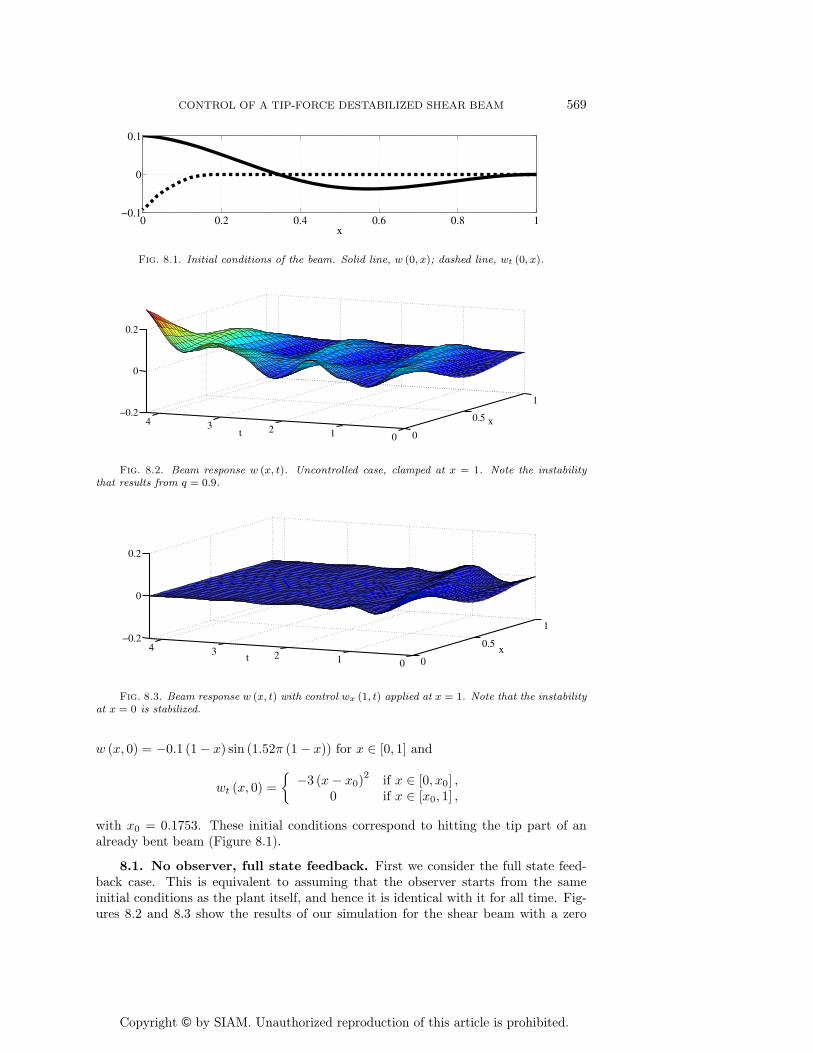
8. Simulation results. In this section we demonstrate through numerical sim-ulations the effectiveness of the control and the observer.

We use the backward Euler method in the time domain and the Chebyshev spec-tral method in space. For this purpose the second-order-in-time equations are firstconverted into first-order-in-time (evolution-type) systems of equations. The controlkernel k is first approximated on a uniform grid using the iterative scheme (3.10),and then linear interpolation was used to obtain values on the nonuniform Chebyshevgrid. The boundary conditions were implemented using second-order explicit dis-cretization. In the numerical simulations we used grid size N = 40 in space and timestep dt = 10−4. The convergence of the numerical method was checked by varyingN between N = 30 and N = 70 and varying dt between dt = 10−2 and dt = 10−5.The maximum variation of the solution did not exceed 10−3 over the whole time andspace domain. The numerical code was programed in MATLAB (see, e.g., [18]).

The main system parameters are set to δ = 1, b = 0.6, and q = 0.9. Thedesign parameters are set to c0 = 10, c1 = 1, and c2 = 1. The initial conditions are



0 0.2 0.4 0.6 0.8 1−0.1

0

0.1

x

Fig. 8.1. Initial conditions of the beam. Solid line, w (0, x); dashed line, wt (0, x).

0

0.5

1

01234−0.2

0

0.2

xt

Fig. 8.2. Beam response w (x, t). Uncontrolled case, clamped at x = 1. Note the instabilitythat results from q = 0.9.

0

0.5

1

01234−0.2

0

0.2

xt

Fig. 8.3. Beam response w (x, t) with control wx (1, t) applied at x = 1. Note that the instabilityat x = 0 is stabilized.

w (x, 0) = −0.1 (1 − x) sin (1.52π (1 − x)) for x ∈ [0, 1] and

wt (x, 0) =

{−3 (x− x0)

2if x ∈ [0, x0] ,

0 if x ∈ [x0, 1] ,

with x0 = 0.1753. These initial conditions correspond to hitting the tip part of analready bent beam (Figure 8.1).

8.1. No observer, full state feedback. First we consider the full state feed-back case. This is equivalent to assuming that the observer starts from the sameinitial conditions as the plant itself, and hence it is identical with it for all time. Fig-ures 8.2 and 8.3 show the results of our simulation for the shear beam with a zero



Uncontrolled Beam Controlled Beam

0 0.2 0.4 0.6 0.8 1−0.1

0

0.1

0.2

0.3

0 0.2 0.4 0.6 0.8 1−0.1

0

0.1

0.2

0.3

t ∈ [0, 0.4] t ∈ [0, 0.4]

0 0.2 0.4 0.6 0.8 1−0.1

0

0.1

0.2

0.3

0 0.2 0.4 0.6 0.8 1−0.1

0

0.1

0.2

0.3

t ∈ [0.4, 1.5] t ∈ [0.4, 1.5]

0 0.2 0.4 0.6 0.8 1−0.1

0

0.1

0.2

0.3

0 0.2 0.4 0.6 0.8 1−0.1

0

0.1

0.2

0.3

t ∈ [1.5, 2.1] t ∈ [1.5, 2.1]

0 0.2 0.4 0.6 0.8 1−0.1

0

0.1

0.2

0.3

0 0.2 0.4 0.6 0.8 1−0.1

0

0.1

0.2

0.3

t ∈ [2.1, 2.8] t ∈ [2.1, 2.8]

0 0.2 0.4 0.6 0.8 1−0.1

0

0.1

0.2

0.3

0 0.2 0.4 0.6 0.8 1−0.1

0

0.1

0.2

0.3

t ∈ [2.8, 3.6] t ∈ [2.8, 3.6]

0 0.2 0.4 0.6 0.8 1−0.1

0

0.1

0.2

0.3

0 0.2 0.4 0.6 0.8 1−0.1

0

0.1

0.2

0.3

t ∈ [3.6, 4.2] t ∈ [3.6, 4.2]

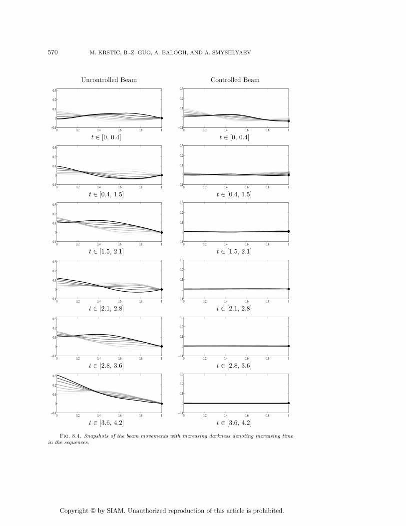
Fig. 8.4. Snapshots of the beam movements with increasing darkness denoting increasing timein the sequences.



Control w (1, t) = u1 (t)

0 1 2 3 4−0.04

−0.02

0

0.02

0.04

time

Control α (1, t) = u2 (t)

0 1 2 3 4

−0.02

0

0.02

0.04

time

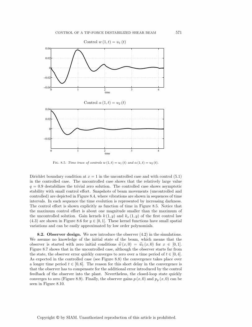
Fig. 8.5. Time trace of controls w (1, t) = u1 (t) and α (1, t) = u2 (t).

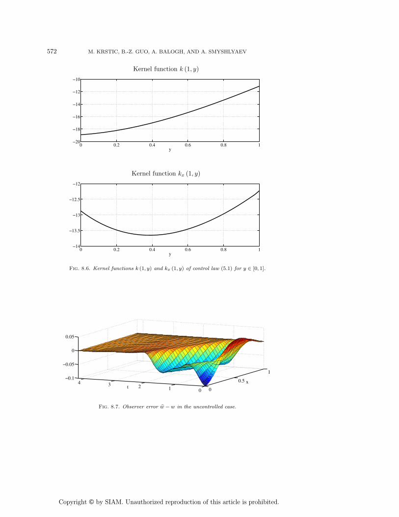
Dirichlet boundary condition at x = 1 in the uncontrolled case and with control (5.1)in the controlled case. The uncontrolled case shows that the relatively large valueq = 0.9 destabilizes the trivial zero solution. The controlled case shows asymptoticstability with small control effort. Snapshots of beam movements (uncontrolled andcontrolled) are depicted in Figure 8.4, where vibrations are shown in sequences of timeintervals. In each sequence the time evolution is represented by increasing darkness.The control effort is shown explicitly as function of time in Figure 8.5. Notice thatthe maximum control effort is about one magnitude smaller than the maximum ofthe uncontrolled solution. Gain kernels k (1, y) and kx (1, y) of the first control law(4.3) are shown in Figure 8.6 for y ∈ [0, 1]. These kernel functions have small spatialvariations and can be easily approximated by low order polynomials.

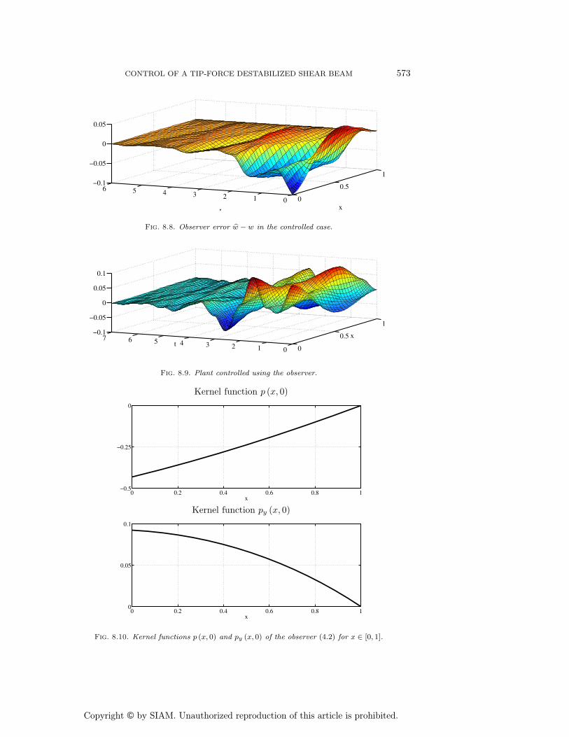
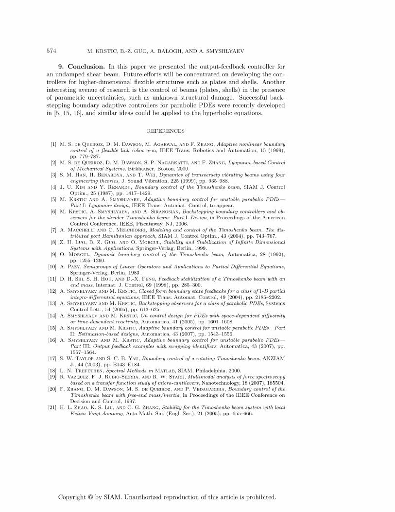
8.2. Observer design. We now introduce the observer (4.2) in the simulations.We assume no knowledge of the initial state of the beam, which means that theobserver is started with zero initial conditions w (x, 0) = wt (x, 0) for x ∈ [0, 1].Figure 8.7 shows that in the uncontrolled case, although the observer starts far fromthe state, the observer error quickly converges to zero over a time period of t ∈ [0, 4].As expected in the controlled case (see Figure 8.8) the convergence takes place overa longer time period t ∈ [0, 6]. The reason for this short delay in the convergence isthat the observer has to compensate for the additional error introduced by the controlfeedback of the observer into the plant. Nevertheless, the closed-loop state quicklyconverges to zero (Figure 8.9). Finally, the observer gains p (x, 0) and py (x, 0) can beseen in Figure 8.10.



Kernel function k (1, y)

0 0.2 0.4 0.6 0.8 1−20

−18

−16

−14

−12

−10

y

Kernel function kx (1, y)

0 0.2 0.4 0.6 0.8 1−14

−13.5

−13

−12.5

−12

y

Fig. 8.6. Kernel functions k (1, y) and kx (1, y) of control law (5.1) for y ∈ [0, 1].

0

0.5

1

01234−0.1

−0.05

0

0.05

xt

Fig. 8.7. Observer error w − w in the uncontrolled case.



0

0.5

1

0123456−0.1

−0.05

0

0.05

xt

Fig. 8.8. Observer error w − w in the controlled case.

0

0.5

1

01234567−0.1

−0.05

0

0.05

0.1

xt

Fig. 8.9. Plant controlled using the observer.

Kernel function p (x, 0)

0 0.2 0.4 0.6 0.8 1−0.5

−0.25

0

x

Kernel function py (x, 0)

0 0.2 0.4 0.6 0.8 10

0.05

0.1

x

Fig. 8.10. Kernel functions p (x, 0) and py (x, 0) of the observer (4.2) for x ∈ [0, 1].



9. Conclusion. In this paper we presented the output-feedback controller foran undamped shear beam. Future efforts will be concentrated on developing the con-trollers for higher-dimensional flexible structures such as plates and shells. Anotherinteresting avenue of research is the control of beams (plates, shells) in the presenceof parametric uncertainties, such as unknown structural damage. Successful back-stepping boundary adaptive controllers for parabolic PDEs were recently developedin [5, 15, 16], and similar ideas could be applied to the hyperbolic equations.

REFERENCES

[1] M. S. de Queiroz, D. M. Dawson, M. Agarwal, and F. Zhang, Adaptive nonlinear boundarycontrol of a flexible link robot arm, IEEE Trans. Robotics and Automation, 15 (1999),pp. 779–787.

[2] M. S. de Queiroz, D. M. Dawson, S. P. Nagarkatti, and F. Zhang, Lyapunov-based Controlof Mechanical Systems, Birkhauser, Boston, 2000.

[3] S. M. Han, H. Benaroya, and T. Wei, Dynamics of transversely vibrating beams using fourengineering theories, J. Sound Vibration, 225 (1999), pp. 935–988.

[4] J. U. Kim and Y. Renardy, Boundary control of the Timoshenko beam, SIAM J. ControlOptim., 25 (1987), pp. 1417–1429.

[5] M. Krstic and A. Smyshlyaev, Adaptive boundary control for unstable parabolic PDEs—Part I: Lyapunov design, IEEE Trans. Automat. Control, to appear.

[6] M. Krstic, A. Smyshlyaev, and A. Siranosian, Backstepping boundary controllers and ob-servers for the slender Timoshenko beam: Part I–Design, in Proceedings of the AmericanControl Conference, IEEE, Piscataway, NJ, 2006.

[7] A. Macchelli and C. Melchiorri, Modeling and control of the Timoshenko beam. The dis-tributed port Hamiltonian approach, SIAM J. Control Optim., 43 (2004), pp. 743–767.

[8] Z. H. Luo, B. Z. Guo, and O. Morgul, Stability and Stabilization of Infinite DimensionalSystems with Applications, Springer-Verlag, Berlin, 1999.

[9] O. Morgul, Dynamic boundary control of the Timoshenko beam, Automatica, 28 (1992),pp. 1255–1260.

[10] A. Pazy, Semigroups of Linear Operators and Applications to Partial Differential Equations,Springer-Verlag, Berlin, 1983.

[11] D. H. Shi, S. H. Hou, and D.-X. Feng, Feedback stabilization of a Timoshenko beam with anend mass, Internat. J. Control, 69 (1998), pp. 285–300.

[12] A. Smyshlyaev and M. Krstic, Closed form boundary state feedbacks for a class of 1-D partialintegro-differential equations, IEEE Trans. Automat. Control, 49 (2004), pp. 2185–2202.

[13] A. Smyshlyaev and M. Krstic, Backstepping observers for a class of parabolic PDEs, SystemsControl Lett., 54 (2005), pp. 613–625.

[14] A. Smyshlyaev and M. Krstic, On control design for PDEs with space-dependent diffusivityor time-dependent reactivity, Automatica, 41 (2005), pp. 1601–1608.

[15] A. Smyshlyaev and M. Krstic, Adaptive boundary control for unstable parabolic PDEs—PartII: Estimation-based designs, Automatica, 43 (2007), pp. 1543–1556.

[16] A. Smyshlyaev and M. Krstic, Adaptive boundary control for unstable parabolic PDEs—Part III: Output feedback examples with swapping identifiers, Automatica, 43 (2007), pp.1557–1564.

[17] S. W. Taylor and S. C. B. Yau, Boundary control of a rotating Timoshenko beam, ANZIAMJ., 44 (2003), pp. E143–E184.

[18] L. N. Trefethen, Spectral Methods in Matlab, SIAM, Philadelphia, 2000.[19] R. Vazquez, F. J. Rubio-Sierra, and R. W. Stark, Multimodal analysis of force spectroscopy

based on a transfer function study of micro-cantilevers, Nanotechnology, 18 (2007), 185504.[20] F. Zhang, D. M. Dawson, M. S. de Queiroz, and P. Vedagarbha, Boundary control of the

Timoshenko beam with free-end mass/inertia, in Proceedings of the IEEE Conference onDecision and Control, 1997.

[21] H. L. Zhao, K. S. Liu, and C. G. Zhang, Stability for the Timoshenko beam system with localKelvin-Voigt damping, Acta Math. Sin. (Engl. Ser.), 21 (2005), pp. 655–666.

Documents

ONTROL OPTIM c