Embed Size (px)
Citation preview

ONTARIO GEOLOGICAL SURVEY
Geophysical Data Set 1249
Ontario Airborne Geophysical Surveys Magnetic and Gravimetric Data Pays Plat Lake Area
by Ontario Geological Survey
2016
Ontario Geological Survey Ministry of Northern Development and Mines Willet Green Miller Centre, 933 Ramsey Lake Road, Sudbury, Ontario P3E 6B5 Canada
© Queen’s Printer for Ontario, 2016
ii
Contents
CREDITS .................................................................................................................................................... iv DISCLAIMER ............................................................................................................................................ iv CITATION .................................................................................................................................................. iv ACKNOWLEDGMENT ............................................................................................................................. iv NOTE ......................................................................................................................................................... iv
1. Introduction .................................................................................................................................................. 1
2. Survey Location and Specifications ............................................................................................................ 1 2.1. Survey Location ............................................................................................................................... 1 2.2. Survey Specifications ...................................................................................................................... 2
3. Aircraft and Personnel ................................................................................................................................ 2 3.1. Aircraft Britten-Norman BN2B-21 Islander .................................................................................... 2 3.2. Personnel ......................................................................................................................................... 3
4. Equipment .................................................................................................................................................... 3 4.1. Airborne Navigation and Data Acquisition System ......................................................................... 3
4.1.1. Sander Geophysics Data Acquisition System (SGDAS) ...................................................... 3 4.2. Airborne Gravity System ................................................................................................................. 4
4.2.1. Sander Geophysics AIRGrav ............................................................................................... 4 4.3. Aerial and Ground Magnetometers.................................................................................................. 4
4.3.1. Geometrics G-822A ............................................................................................................. 4 4.4. Magnetic Compensation System ..................................................................................................... 4
4.4.1. Sander Geophysics AIRComp ............................................................................................. 4 4.5. Reference Station Acquisition System ............................................................................................ 4
4.5.1. Sander Geophysics SGRef ................................................................................................... 4 4.5.2. Sander Geophysics MSGRef ................................................................................................ 5
4.6. GNSS and GPS Receivers ............................................................................................................... 5 4.6.1. NovAtel® OEMV-3 Receiver Board .................................................................................... 5 4.6.2. NovAtel® OEM3 or OEM4 Receiver Boards ....................................................................... 5
4.7. Altimeters ........................................................................................................................................ 5 4.7.1. SGLas-P – Riegl LD90-31K-HiP Laser Rangefinder .......................................................... 5 4.7.2. Bendix King KRA-10A Radar Altimeter ............................................................................. 5
5. Pre-acquisition Tests .................................................................................................................................... 6 5.1. Gravity System Tests ....................................................................................................................... 6
5.1.1. Gravity Quality Assessment (Ottawa Gravity Repeat Lines) ............................................... 6 5.2. Magnetometer System Tests ............................................................................................................ 6
5.2.1. Magnetometer Heading Test ................................................................................................ 6 5.2.2. Compensation Calibration .................................................................................................... 6 5.2.3. Lag Test................................................................................................................................ 6 5.2.4. Magnetometer Sensor Comparison Test .............................................................................. 6

iii
5.3. Altimeter System ............................................................................................................................. 6 5.3.1. Radar and Laser Altimeter Calibration ................................................................................ 6
6. Data Acquisition ........................................................................................................................................... 7 6.1. Magnetic Data ................................................................................................................................. 7 6.2. Gravity Data .................................................................................................................................... 7 6.3. Digital Elevation Data ..................................................................................................................... 8
7. Contractor Processing ................................................................................................................................. 8 7.1. Magnetic Data Processing ............................................................................................................... 8 7.2. Gravity Data Processing .................................................................................................................. 9
7.2.1. Gridding and Filtering .......................................................................................................... 10 7.3. Digital Elevation .............................................................................................................................. 11
8. Final Data Compilation and Processing ..................................................................................................... 11 8.1. Base Maps ....................................................................................................................................... 11
8.1.1. Projection Description .......................................................................................................... 11 8.2. Magnetic Processing ........................................................................................................................ 11
8.2.1. Microlevelling and Gridding ................................................................................................ 11 8.2.2. Levelling Magnetic Data to Master Magnetic Datum .......................................................... 12 8.2.3. Second Vertical Derivative Magnetic Grid .......................................................................... 12 8.2.4. Keating Correlation Coefficients.......................................................................................... 12
8.3. Gravity Processing ........................................................................................................................... 14 8.3.1. Gravity Grids ........................................................................................................................ 14
8.4. Digital Elevation Model .................................................................................................................. 14 8.5. Map Products ................................................................................................................................... 14
8.5.1. Digital Maps Sets ................................................................................................................. 14 8.5.2. Final Map Products .............................................................................................................. 14
8.6. Creation of Georeferenced Geotiff Images ...................................................................................... 15 8.7. Creation of Linework (Vector) Archives ......................................................................................... 15
9. References ..................................................................................................................................................... 15 Appendix A. Data Files Description ................................................................................................................ 16
Appendix B. Magnetic Profile Archive Definition ......................................................................................... 18
Appendix C. Gravity Profile Archive Definition ........................................................................................... 19
Appendix D. Keating Correlation Archive Definition ................................................................................... 20
Appendix E. Grid Archive Definition ............................................................................................................. 21
Appendix F. GeoTIFF and Vector Archive Definition .................................................................................. 22
FIGURES 1. Location of the Pays Plat Lake area survey ................................................................................................ 1 2. Flight paths for the Pays Plat Lake area survey .......................................................................................... 2
3. Total field response of the model used in Keating correlations .................................................................. 13

iv
CREDITS List of accountabilities and responsibilities.
• Nuclear Waste Management Organization (NWMO), Toronto, Ontario – commissioned and paid for the survey
• Jack Parker, Senior Manager, Earth Resources and Geoscience Mapping Section, Ontario Geological Survey (OGS), Ministry of Northern Development and Mines (MNDM) – accountable for the geophysical survey projects, including contract management
• Steve Munro, Senior Geophysicist, Scott Hogg & Associates Ltd. (SHA), Toronto, Ontario – responsible for the reprocessing of this data set
• Tom Watkins, Manager, Publication Services Unit, GeoServices Section, Ontario Geological Survey, MNDM – managed the project-related hard-copy products
• Desmond Rainsford, Geophysicist, Earth Resources and Geoscience Mapping Section, Ontario Geological Survey – responsible for initial quality assurance (QA), quality control (QC) and project-related digital products
• Sander Geophysics Ltd, Ottawa, Ontario – data acquisition and original products
DISCLAIMER Every possible effort has been made to ensure the accuracy of the information presented in this report and the accompanying data; however, the Ministry of Northern Development and Mines does not assume liability for errors that may occur. Users should verify critical information.
The geophysical data were acquired from another organization. The original data acquisition was neither supervised by the Ontario Geological Survey (OGS) nor carried out to OGS technical specifications. However, the data do meet a pre-defined valuation criteria set out by the OGS. Some quality assurance and quality control checks have been carried out on the digital data.
CITATION Information from this publication may be quoted if credit is given. It is recommended that reference be made in the following form: Ontario Geological Survey 2016. Survey report on Pays Plat Lake area, 22p. [PDF document]; in Ontario airborne
geophysical surveys, magnetic and gravimetric data, grid and profile data (ASCII and Geosoft® formats) and vector data, Pays Plat Lake area, Ontario Geological Survey, Geophysical Data Set 1249.
ACKNOWLEDGMENT The geophysical data that comprise this survey were generously donated by Nuclear Waste Management Organization (NWMO). The survey was flown for NWMO under the original name of “Schreiber Block”.
NOTE
Users of OGS products are encouraged to contact those Aboriginal communities whose traditional territories may be located in the mineral exploration area to discuss their project.

Report on Pays Plat Lake Area Airborne Geophysical Survey
Geophysical Data Set 1249 p.1
1. Introduction As part of an on-going program to acquire high-quality, high-resolution airborne geophysical data across the Province of Ontario, the Ministry of Northern Development and Mines (MNDM) does, from time to time, acquire existing proprietary existing data. Acquisition of existing data complements new surveys commissioned by the MNDM. This data set was kindly donated by the Nuclear Waste Management Organization (NWMO). The data were collected by the NWMO in the Schreiber area. The name of the survey area was changed to Pays Plat Lake Area to avoid confusion with a previously published Schreiber airborne geophysical survey.
2. Survey Location and Specifications
2.1. SURVEY LOCATION This report describes a fixed-wing magnetic and gravity survey carried out near Schreiber, Ontario, on the north shore of Lake Superior. The survey was conducted by Sander Geophysics Ltd. (SGL), Ottawa, Ontario, for the Nuclear Waste Management Organization of Toronto, Ontario. The survey was flown during the period April 12 to 24, 2014, and 3432 line-kilometres of magnetic and gravimetric data were collected.
The survey block was located approximately 15 km north of the community of Schreiber, Ontario (approximately 150 km east-northeast of Thunder Bay, Ontario) (Figure 1).
Figure 1. Location of the Pays Plat Lake area survey.

Report on Pays Plat Lake Area Airborne Geophysical Survey
Geophysical Data Set 1249 p.2
2.2. SURVEY SPECIFICATIONS The survey was flown using an east-west line direction with 100 m line spacing. Tie-lines were flown in a north-south direction, at 500 m spacing. The tie lines were alternately extended by a distance of 5 km from the north and south boundaries of the core survey area. Additionally, every tenth survey line was extended out 5 km from each side of the core survey area, creating a coarse surrounding region of one-kilometre-spaced coverage (Figure 2). The total survey coverage was 3432 line-kilometres. Throughout the survey, the aircraft maintained a nominal altitude of 80 m.
Figure 2. Flight paths for the Pays Plat Lake area survey.
3. Aircraft and Personnel
3.1. AIRCRAFT BRITTEN-NORMAN BN2B-21 ISLANDER The BN2B Islander is an all-metal, high-wing, twin-engine, short take-off and landing aircraft powered by 2 fuel-injected engines which drive constant speed, fully feathering propellers. The aircraft has fixed tricycle landing gear, extendable flaps and manually adjustable trim tabs on the rudder and elevator. The aircraft is equipped with de-icing equipment and sufficient avionics for instrument flying. There is a camera hole in the belly of the aircraft and provisions for numerous other survey and navigation systems. The airframe has been extensively modified to reduce the magnetic signature of the aircraft by replacing ferromagnetic parts with those made from special non-magnetic stainless steel or aluminum. Several wiring changes have also been made to the electrical system to reduce the magnetic field variations around the aircraft. Other extensive modifications have been made to allow for gravity, spectrometer,

Report on Pays Plat Lake Area Airborne Geophysical Survey
Geophysical Data Set 1249 p.3
LiDAR and methane-sensing surveys. Because of its low take-off speed, high wing, ample propeller clearance, and sturdy fixed landing gear, the Islander is capable of operating from relatively short and rough airstrips. Its excellent low-speed capabilities enable it to safely contour much steeper terrain than most other fixed-wing aircraft. All survey modifications are certified to meet the requirements of the Canadian Aviation Regulations (CARs).
3.2. PERSONNEL The following personnel were involved with the survey.
Field Field Crew Chief: Adam Jones Data Processor: Noah Dewar Pilot: Steven Hyde Co-Pilot: Jeremy Anderson Aircraft Maintenance Engineer: Dax Jutras Technician: Lee Duncan
Office Project Manager: Reed Archer Field Project Manager: Al Pritchard
4. Equipment Sander Geophysics Ltd. provided the following instrumentation for this survey:
4.1. AIRBORNE NAVIGATION AND DATA ACQUISITION SYSTEM
4.1.1. SANDER GEOPHYSICS DATA ACQUISITION SYSTEM (SGDAS) The SGDAS is the latest version of airborne navigation and data acquisition computers developed by Sander Geophysics. It is the data gathering core for all the different types of survey data. The computer incorporates a magnetometer coupler, an altimeter analog to digital converter and a NovAtel® global positioning system (GPS) multi-frequency receiver (for details, see “4.6. GNSS and GPS Receivers”), which automatically provides the UTC time base for the recorded data. The system acquires the different data streams from the sensors and receives and processes GPS signals from the GPS antenna. Navigation information from the navigation side of the computer guides the pilots along the pre-planned flight path in all 3 dimensions. Profiles of the incoming data are displayed in real-time to the pilots for continuous monitoring. The data are recorded in database format on redundant solid-state data storage modules. The AIRGrav system (see “4.2.1. Sander Geophysics AIRGrav”) incorporates an additional data acquisition system: gravity DAS (GDAC). The GDAC controls the AIRGrav system, has its own GPS receiver for position and time, records the data collected, and includes a separate user interface.

Report on Pays Plat Lake Area Airborne Geophysical Survey
Geophysical Data Set 1249 p.4
4.2. AIRBORNE GRAVITY SYSTEM
4.2.1. SANDER GEOPHYSICS AIRGRAV Sander Geophysics’ airborne inertially referenced gravimeter system, AIRGrav, uses a Schuler-tuned inertial platform. This platform supports 3 orthogonal accelerometers, which remain fixed in inertial space, independent of the manoeuvres of the aircraft, allowing precise correction of the effects of the movement of the aircraft. Accelerometer data are recorded at 128 Hz and later down sampled to 2 Hz in processing. The gravity sensor used in AIRGrav is a very accurate accelerometer with a wide dynamic range. The system is not affected by the strong vertical motions of the aircraft, allowing the final gravity data to be almost completely unaffected by aircraft dynamics up to what is considered “moderate” turbulence. The instrument is also rendered as an inertial navigator and, as such, the platform levelling is essentially unaffected by horizontal accelerations. Gravity data are consistently acquired with a noise level of less than 0.2 mGal with a half sine wave ground resolution of 1.8 to 2 km, given adequate line spacing.
4.3. AERIAL AND GROUND MAGNETOMETERS
4.3.1. GEOMETRICS G-822A Both the ground and airborne systems used a non-oriented (strap-down) optically pumped cesium split-beam sensor. These magnetometers have a sensitivity of 0.005 nT and a range of 20 000 to 100 000 nT with a sensor noise of less than 0.0005 nT. The airborne sensor was mounted in a fibreglass stinger extending from the tail of the aircraft. Total magnetic field measurements were recorded at 160 Hz in the aircraft, and then later downsampled to 10 Hz in the processing. The ground systems recorded magnetic data at 1 Hz.
4.4. MAGNETIC COMPENSATION SYSTEM
4.4.1. SANDER GEOPHYSICS AIRCOMP Sander Geophysics’ own hardware and software system, AIRComp, was used to remove the effects of the aircraft and its manoeuvres from the recorded magnetic data. This system records the magnetic field measured by up to 4 cesium magnetometers, as well as the three-axis output of a fluxgate magnetometer. These data are recorded for post-processing. Calibration of the magnetic effects of the aircraft is carried out as described in “5.2. Magnetometer System Tests”. Coefficients to be used for compensation are derived by processing the calibration flight data. The compensation coefficients are applied to data recorded during normal survey operations to produce compensated magnetic data.
4.5. REFERENCE STATION ACQUISITION SYSTEM
4.5.1. SANDER GEOPHYSICS SGREF Sander Geophysics’ reference (ground) station, SGRef, is a dual reference station. One half consists of a data acquisition computer with a cesium magnetometer interface and frequency counter to process the signal from the magnetometer sensor and from the GPS receiver (for details, see “4.6. GNSS and GPS Receivers”). The other half contains only a GPS receiver. These 2 halves operate independently of each other. The time base (UTC) of both the ground and airborne systems is automatically provided by the GPS receiver, ensuring proper merging of both data sets. All data are displayed on an LCD flat-panel monitor.

Report on Pays Plat Lake Area Airborne Geophysical Survey
Geophysical Data Set 1249 p.5
4.5.2. SANDER GEOPHYSICS MSGREF The MSGRef (mini SGRef) consists of a data acquisition computer with a cesium magnetometer interface and frequency counter to process the signal from the magnetometer sensor and from the GPS receiver (for details, see “4.6. GNSS and GPS Receivers”). All data are displayed on an LCD flat-panel monitor. The GPS data, sampled at 10 Hz, are recorded on the internal hard drive of the computer and the removable hard drive simultaneously for transfer to the processing computers in the field office. The magnetic data, sampled at 10 Hz, are also recorded to both hard drives. The entire reference data acquisition system was set for automatic, unattended recording. The noise level of the reference station magnetometer is less than 0.1 nT.
4.6. GNSS AND GPS RECEIVERS
4.6.1. NOVATEL® OEMV-3 RECEIVER BOARD The NovAtel® OEMV-3, multi-frequency GNSS (global navigation satellite system) receiver is configurable up to 72 channels with the tracking of GPS (L1, L2, L5), GLONASS (L1, L2), SBAS, and L-band satellites and signals. It provides averaged position and raw range information of all satellites in view. The GNSS positional data are recorded at 10 Hz.
4.6.2. NOVATEL® OEM3 OR OEM4 RECEIVER BOARDS The OEM3 is a high-performance, high-accuracy, dual-frequency GPS receiver that is capable of receiving and tracking the L1 C/A code, L1 and L2 carrier phase, and L2 P-code (or encrypted Y-code) of up to 24 GPS satellites. The GPS data are recorded at 10 Hz.
4.7. ALTIMETERS
4.7.1. SGLAS-P – RIEGL LD90-31K-HIP LASER RANGEFINDER The Riegl laser altimeter uses a single optical laser beam to measure distance to the ground. It is effective over water and is eye safe. This profilometer has a range of 1500 m, a resolution of 0.01 m with an accuracy of 5 cm and a 3.3 Hz data rate.
4.7.2. BENDIX KING KRA-10A RADAR ALTIMETER The Bendix King radar altimeter has a resolution of 0.5 m, an accuracy of 5%, a range of 6 to 760 m, and a 10 Hz data rate. This system is employed as a backup system and not actively employed for survey guidance or data processing.

Report on Pays Plat Lake Area Airborne Geophysical Survey
Geophysical Data Set 1249 p.6
5. Pre-acquisition Tests
5.1. GRAVITY SYSTEM TESTS
5.1.1. GRAVITY QUALITY ASSESSMENT (OTTAWA GRAVITY REPEAT LINES) Prior to field deployment, the AIRGrav system was tested by flying several passes over SGL’s established Ottawa gravity repeat line. On March 26, the aircraft flew 6 such passes over the test line and all passes had standard deviations lower than 0.5 mGal.
5.2. MAGNETOMETER SYSTEM TESTS
5.2.1. MAGNETOMETER HEADING TEST A test flight was performed to measure the heading error of the magnetic system in the survey aircraft using the Geological Survey of Canada (GSC) Bourget test site on March 26. The test determined an average north-south heading error of 0.90 nT, an average east-west heading error of -0.59 nT and an absolute error of 0.05 nT.
5.2.2. COMPENSATION CALIBRATION A compensation calibration to determine the magnetic influence of the aircraft and its manoeuvres was flown on April 3 in Hearst, Ontario. The resulting Figure of Merit (FOM) was calculated to be 1.07 nT.
5.2.3. LAG TEST A lag test was flown on March 3 prior to field deployment and showed that the instrumentation lag was well corrected using the expected parameters.
5.2.4. MAGNETOMETER SENSOR COMPARISON TEST The magnetic data recorded by the plane was compared to the data recorded by the base station and both showed to be in very good agreement.
5.3. ALTIMETER SYSTEM
5.3.1. RADAR AND LASER ALTIMETER CALIBRATION A test flight to calibrate the radar and laser altimeters was flown prior to survey commencement on March 30 over the Hearst Airport runway. All altimeters were shown to have an accuracy of better than 2%.

Report on Pays Plat Lake Area Airborne Geophysical Survey
Geophysical Data Set 1249 p.7
6. Data Acquisition
6.1. MAGNETIC DATA Total magnetic field measurements were recorded with a single cesium magnetometer mounted in a fibreglass stinger extending from the tail of the survey aircraft. Sander Geophysics’ hardware and software system, AIRComp, was used to remove the effects of the aircraft and its manoeuvres from the recorded magnetic data. The data were recorded for post-processing. Coefficients to be used for compensation were derived by processing the calibration flight data, based on principles presented by Leliak (1961). The compensation coefficients were applied to data recorded during normal survey operations to produce compensated magnetic data.
Both the ground and airborne systems used the Geometrics Ltd. G-822A cesium magnetic sensor. Total magnetic field measurements were recorded at 160 Hz in the aircraft, and then later downsampled to 10 Hz in processing. The ground systems recorded magnetic data at 1 Hz.
A pre-planned drape surface was prepared for the survey to guide the aircraft over the topography in a consistent manner, as close to the minimum clearance as possible. The drape surface was prepared with digital elevation model (DEM) data obtained from the Shuttle Radar Topography Mission (SRTM) for the area. The DEM included an extension beyond the survey boundary to allow the aircraft to achieve the drape clearance before coming online.
6.2. GRAVITY DATA Gravity data were acquired with Sander Geophysics’ propriety AIRGrav (airborne inertially referenced gravimeter) system, which uses a Schuler-tuned inertial platform supporting 3 orthogonal accelerometers, which remain fixed in inertial space, independent of the manoeuvres of the aircraft, allowing precise isolation from the effects of the movement of the aircraft. The gravity sensor used in AIRGrav is a very accurate accelerometer with a wide dynamic range. The system is not affected by the strong vertical motions of the aircraft, allowing the final gravity data to be almost completely unaffected by in-flight conditions classified as “moderate turbulence” or better. The instrument is also considered to be an inertial navigator and. as such. the platform levelling was essentially unaffected by horizontal accelerations.
In typical survey flying, accelerations in an aircraft can reach 0.1 G, equivalent to 100 000 mGal. Data processing must extract gravity data from this very noisy environment. This was achieved by modelling the gravity resulting from movements of the aircraft in flight as measured by extremely accurate GPS measurements. These measurements are affected by noisy conditions in the ionosphere, and by the variable conditions (e.g., temperature, pressure and humidity) within the troposphere. Sander Geophysics has developed a full suite of programs to carry out all the necessary corrections.
The GPS data were extracted from the airborne and reference station acquisition system and reformatted. Differential corrections to correct the airborne ranges for variations calculated from the base station GPS data were performed. Each recorded position was recalculated based on these ranges. The original reference system for all GPS data was the World Geodetic System 1984 (WGS84) datum. Positions were then converted to the local datum, reference system and desired projection. Each line was then checked for data continuity and quality.
An extremely accurate location of the base station GPS receiver was determined using an International GNSS Service (IGS) permanent GPS Reference Station to apply differential corrections (http://igs.org/network). This technique provides a final base station receiver location with an accuracy of better than a few decimetres. The entire airborne data set was then reprocessed differentially using the recalculated base station location.

Report on Pays Plat Lake Area Airborne Geophysical Survey
Geophysical Data Set 1249 p.8
Gravity data were recorded at 128 Hz. Accelerations were filtered and resampled to 10 Hz to match the GPS, using specially designed filters to avoid biasing the data. Gravity was calculated by subtracting the GPS derived accelerations from the inertial accelerations. The calculated gravity was corrected for the Eötvös effect and normal gravity, and the sample interval was then reduced to 2 Hz.
6.3. DIGITAL ELEVATION DATA Digital elevation data were collected during the survey using a laser altimeter (Riegl LD90-31K-HiP) mounted to the base of the aircraft. The elevation data were sampled at a rate of 3.3 Hz, which is consistent with a sample approximately every 16 m along the profile line. Even though the laser altimeter can record returns from more than 700 m above the ground with a high degree of certainty, some laser data dropouts occurred while flying over the areas of poor reflectivity. The laser data show the effects of the dense tree cover: variable penetration of the canopy results in a high frequency variation of recorded altitude. The raw laser data were processed with an iterative de-spiking routine designed to remove many of the early laser returns from trees.
Digital elevation data were also collected using a King KRA-10 radar altimeter mounted to the base of the aircraft. Data were sampled at a rate of 10 Hz, which is consistent with a sample roughly every 6 m. The radar data penetrates the canopy less as it records the first return within the footprint of its signal. The radar altimeter data were filtered to remove high-frequency noise using a 67-point low-pass filter.
7. Contractor Processing
7.1. MAGNETIC DATA PROCESSING The airborne magnetometer data were recorded at 160 Hz, and downsampled to 10 Hz for processing. A second-order Butterworth 0.9 Hz low-pass filter was utilized in the process for compensation and anti-aliasing. All magnetic data were plotted and checked for any spikes or noise. A 0.244 second static lag correction due to signal processing, in addition to a dynamic lag correction, was applied to each data point. The aircraft speed dependent dynamic lag was calculated using Sander Geophysics’ Dynlag software.
Ground magnetometer data were inspected for cultural interference and edited where necessary. All reference station magnetometer data were filtered using a 121-point low-pass filter to remove any high-frequency noise, but to retain the low-frequency diurnal variations.
A correction for the International Geomagnetic Reference Field (IGRF) was applied to the diurnally corrected profile data. The altitude and horizontal positional GPS data were used to calculate an IGRF profile (using a 2010 IGRF model).
Intersections between control and traverse lines were determined by a program that extracts the magnetic, altitude, and x and y values of the traverse and control lines at each intersection point. Each control line was adjusted by a constant value to minimize the intersection differences, calculated as follows:
∑ |𝑖 − 𝑎| summed over all traverse lines,
where i = (individual intersection difference) a = (average intersection difference for that traverse line)

Report on Pays Plat Lake Area Airborne Geophysical Survey
Geophysical Data Set 1249 p.9
Adjusted control lines were further corrected locally to minimize any residual differences. Traverse-line levelling was done using a program called CLEVEL that interpolates and extrapolates levelling values for each point based on the 2 closest differences at intersections. After traverse lines were levelled, the control lines were matched to them. This ensured that all intersections tie perfectly and permitted the use of all data in the final products.
A curved correction using a function similar to spline interpolation was provided from the CLEVEL program. A third-degree polynomial was used to interpolate between 2 intersections. CLEVEL is an improved method, as it allows intersection points to be preserved with no mismatch and interpolation is smooth with the first derivative continuously approaching the same value from both sides of the intersection points.
The levelling procedure was verified through inspection of the magnetic anomaly and vertical derivative grids by plotting profiles of corrections along lines, and by examination of levelling statistics to check for steep correction gradients.
7.2. GRAVITY DATA PROCESSING The following standard corrections were applied to the gravity data.
a) Eötvös correction,
δgEötvös = − 𝑉𝑋2𝑟
(1 - 𝑒2𝑠𝑖𝑠2𝜑)1 2� + ℎ
− 2𝑊𝑠𝑣𝑥co𝑠𝜑 − 𝑣𝑦2
𝑟(1 − 𝑒2)(1 − 𝑒2𝑠𝑖𝑠2𝜑)3 2�
+ ℎ
where 𝜑 is the latitude of the aircraft, 𝑣𝑋 and 𝑣𝑦 are the velocities of the aircraft in the x (east) and y (north) direction, r is the Earth’s radius at the equator (6,378,137 m), 𝑒2 is a correction for Earth’s flattening towards the poles (6.69437999013 ×10⁻³), 𝑊𝑠 is the angular velocity of Earth’s rotation (7.2921158553 ×10⁻⁵ rad/s), and ℎ is the altitude of the plane above the WGS84 datum.
b) Normal gravity, 𝑔𝑁𝑁𝑁𝑁𝑁𝑁
𝑔𝑁𝑁𝑁𝑁𝑁𝑁 = 9.7803267714 (1 + 0.00193185138639𝑠𝑖𝑠2𝜑)
�1 − 0.00669437999013𝑠𝑖𝑠2𝜑
where 𝜑 is the latitude of the aircraft;
c) Free air correction, 𝑔𝑓𝑁
𝑔𝑓𝑁 = −(0.3087691− 0.0004398𝑠𝑖𝑠2𝜑)ℎ + 7.2125 × 10⁻⁸ℎ2
where 𝜑 is the latitude of the aircraft and ℎ is the height of the aircraft is metres above the WGS84 datum.
d) Bouguer slab correction, 𝑔𝑠𝑠 𝑔𝑠𝑠 = 2𝜋𝜋𝜋ℎ = 0.041925𝜋ℎ
where 𝜋 is the Universal Gravity constant, 𝜋 is the average density for the project in g/cm3 and ℎ is the height of the surface of land or sea in metres above the WGS83 datum.

Report on Pays Plat Lake Area Airborne Geophysical Survey
Geophysical Data Set 1249 p.10
e) Curvature of the Earth, 𝑔𝑒𝑒
𝑔𝑒𝑒 = 𝜋
2.67[ 1.464ℎ − 0.3533ℎ2 + 0.000045ℎ3]
where ℎ is height of the surface of land or sea in kilometres above the WGS84 datum and 𝜋 is the density for the project.
f) Full Bouguer correction, 𝑔𝑠 Shuttle Radar Terrain Mission (SRTM) digital elevation model data were used to calculate the Bouguer corrections for gravity processing. The SRTM data contains information in a grid with a 3 arcsecond spacing, approximately equal to 100 m cell spacing, which has a higher density than the line spacing for this survey and, therefore, provides terrain data at a better resolution between the survey lines. Coverage up to 160 km from the survey block was kept for accurate regional corrections.
Terrain corrections were computed using software developed by Sander Geophysics. The algorithm calculates the topographic attraction of the terrain using a mass prism model with a constant density. The difference between the topographic attraction and the simple Bouguer correction is the terrain correction. The terrain and Bouguer corrections were calculated for the bedrock at the height of the aircraft using densities of 2.67 and 2.40 g/cm3.
g) Static correction, 𝑔𝑠𝑒 A single constant shift, determined from ground static recordings, was applied on a flight-by-flight basis. The pre- and post-flight readings were averaged for each flight and the difference between the average value and the local gravity value was removed. This acts as a simple, but effective, coarse levelling of the data.
h) Level correction, 𝑔𝑁𝑒 Intersection statistics were then used to adjust individual survey lines. Unlike magnetic levelling, individual intersections were not used to make corrections. Instead, intersection differences from whole lines were averaged and a single adjustment was applied to each survey line and each control line. Minor adjustments were calculated for sections of each line based on statistics from groups of intersections. The adjustments were smoothed and applied to line data that was filtered, as described below. Grids of adjusted data were inspected to determine that the adjustments were appropriate.
The final Bouguer anomaly equals G − 𝑔𝑓𝑁 − 𝑔𝑠 − 𝑔𝑠𝑒 − 𝑔𝑁𝑒 where G is the calculated gravity adjusted for Eötvös effect and normal gravity.
7.2.1. GRIDDING AND FILTERING Statistical noise in the data was reduced by applying a cosine tapered low-pass filter to the time-series line data. For this survey, a 20 second (1000 m) half-wavelength filter was employed. The data were gridded using a minimum curvature algorithm that averages all values within any given grid cell and interpolates the data between survey lines to produce a smooth grid. The algorithm produces a smooth grid by iteratively solving a set of difference equations by minimizing the total second horizontal derivative while attempting to honour the input data (Briggs 1974). Grids were generated using a 25 m grid cell size.
Low-pass spatial filtering was applied to the grid to achieve better noise reduction than by simply increasing the degree of line filtering. A range of grid filters were used and evaluated for their effectiveness in removing noise from the data, and highlighting signal content. The final data was filtered with a 1.0 km half-wavelength grid filter.
Report on Pays Plat Lake Area Airborne Geophysical Survey
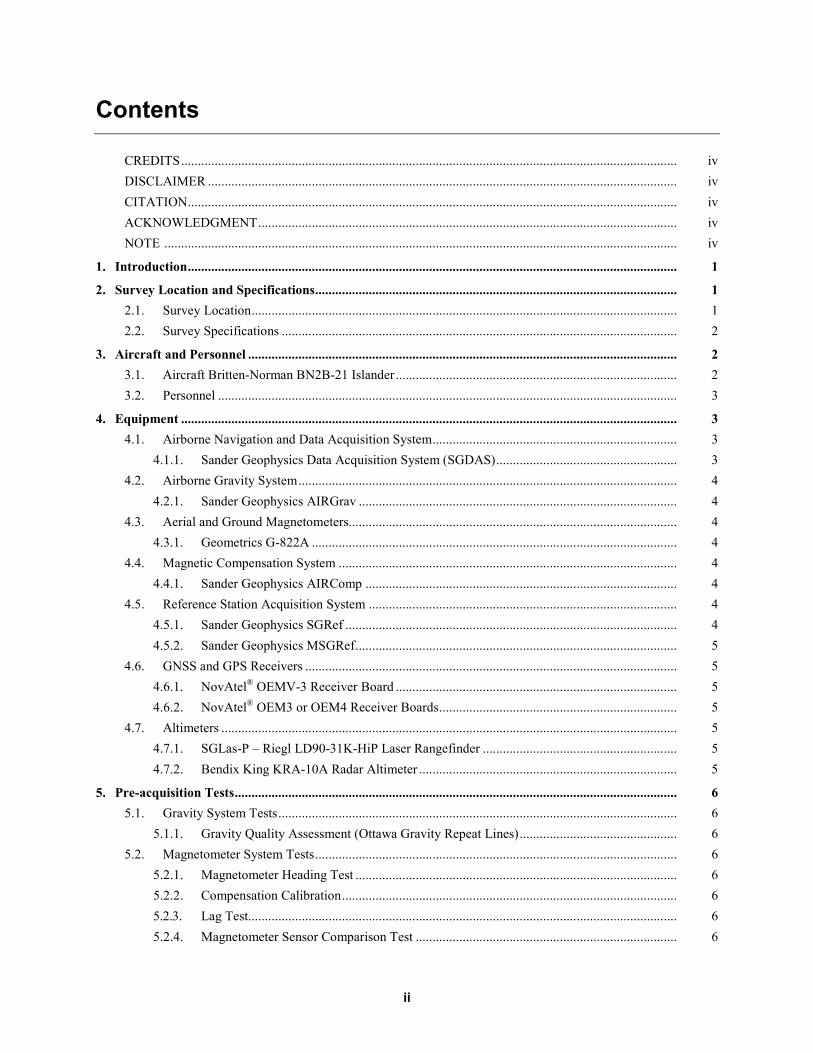
Geophysical Data Set 1249 p.11
7.3. DIGITAL ELEVATION A digital elevation model (DEM) was derived by subtracting the laser altimeter data from the differentially corrected DGPS altitude with respect to the Canadian Geodetic Vertical Datum 2013 (CGVD2013). Short sections of poor laser data resulting from locally weak reflectivity were replaced using King radar altimeter data. The DEM reflects the presence of vegetation (e.g., trees) and buildings and, thus, is not considered to be a digital terrain model (DTM).
8. Final Data Compilation and Processing
8.1. BASE MAPS Base maps of the survey area were supplied by the Ontario Ministry of Northern Development and Mines.
8.1.1. PROJECTION DESCRIPTION Datum: NAD83 (Canada) Ellipsoid: GRS80 Projection: UTM Zone 16N (central meridian = 87°W) False Northing: 0 m False Easting: 500 000 m Scale factor: 0.9996
8.2. MAGNETIC PROCESSING The contractor provided the final magnetic profile database as an ASCII file. With the exception of the latitude and longitude channels, the data was limited to 2 digits of precision. The ASCII file was imported into a Geosoft® format database for processing. It was discovered that the database contained irregularly timed fiducials that deviated from the 0.1 second nominal and varied between 0.09 and 0.11 seconds. This variation was only observed to consistently affect some fiducial increments and the 1 second and 0.5 second fiducials were always correct. Calculation of aircraft velocities using the uncorrected fiducials showed apparent accelerations and decelerations over the intervals were the fiducials deviated from 0.1 second. By rounding the fiducials to the nearest 0.1 second, the apparent velocity variations were eliminated. This indicated that the timing interval was consistent and correct, but that there was a precision error in recording the fiducials. The rounded fiducials were used to replace the original fiducial values.
8.2.1. MICROLEVELLING AND GRIDDING The contractor’s tie-line network levelled mag channel, mag_lev, had been corrected for diurnal variation and IGRF. This channel was used as input to the microlevelling procedure. Microlevelling is the process of removing residual flight-line noise that remains after conventional levelling using control lines. It has become increasingly important as the resolution of aeromagnetic surveys has improved and the requirement of interpreting subtle geophysical anomalies has become more important.
To isolate and remove this noise, the following procedure was employed. An elliptical reject filter, aligned with the flight lines, was first applied to the gridded total magnetic field. This filter removes features with a long wavelength in the flight-line direction, but a short wavelength in the transverse direction. While removing the unwanted residual levelling errors, it also significantly distorts higher amplitude anomalies.

Report on Pays Plat Lake Area Airborne Geophysical Survey
Geophysical Data Set 1249 p.12
In order to minimize the effect on geological anomalies, the flight path was “threaded” through the filtered grid and a database profile channel was created from the filtered grid. The difference between the mag_lev and this filtered profile was calculated. The difference profile was clipped to the amplitude of the observed noise in the grid. A half cosine roll-off filter was then applied to this channel and a final correction profile was derived with wavelengths on the order of 1 km or longer. This microlevel correction profile was applied to the mag_lev profile data and a final magnetic profile channel was created: mag_final. The final mag channel was then gridded using a bi-directional Akima spline.
8.2.2. LEVELLING MAGNETIC DATA TO MASTER MAGNETIC DATUM The final step in the magnetic processing was to level the data set to the 200 m Ontario Master grid, which has been compiled and levelled to the 812.8 m magnetic datum from the Geological Survey of Canada (GSC). The levelling process must retain all the detail of the newer low-altitude survey and only make corrections on the order of 10 km or longer. To accomplish this, a variation on a method developed by Patterson, Grant and Watson (Reford et al. 1990) was used. The procedure was as follows.
The final total magnetic data were gridded at a 200 m cell size and upward continued to a height of 305 m, to match the nominal terrain clearance of the Ontario master grid (Ontario Geological Survey 1999). The difference between the upward-continued grid and the Ontario master grid was calculated. A fast Fourier transform two-dimensional low-pass filter was applied to a grid of the difference, which retained wavelengths longer than 15 km. This filtered grid was re-gridded at a 20 m cell size and the flight path was threaded through the grid to create a correction profile. This long wavelength correction profile was subtracted from the final magnetic channel to create a “GSC-levelled” (mag_gsclevel) channel. The levelled magnetic profile data were then gridded using a bi-directional Akima spline.
8.2.3. SECOND VERTICAL DERIVATIVE MAGNETIC GRID The second vertical derivative of the total magnetic field was computed to enhance small and weak near-surface anomalies and as an aid to delineate the contacts of the lithologies having contrasting magnetic susceptibilities. The location of contacts or boundaries is usually traced by the zero contour of the second vertical derivative map.
The calculation was done in the frequency domain by combining the transfer function of the second vertical derivative and a half-cosine roll-off filter (100 m cutoff wavelength) to minimize grid aliasing effects in the total magnetic field, which are emphasized by the second vertical derivative.
8.2.4. KEATING CORRELATION COEFFICIENTS Possible kimberlite targets are identified from the residual magnetic intensity data, based on the identification of roughly circular anomalies. This procedure is automated by using a known pattern recognition technique (Keating 1995), which consists of computing, over a moving window, a first-order regression between a vertical cylinder model anomaly and the gridded magnetic data. Only the results where the absolute value of the correlation coefficient is above a threshold of 75% were retained. On the magnetic maps, the results are depicted as circular symbols, scaled to reflect the correlation value. The most favourable targets are those that exhibit a cluster of high amplitude solutions. Correlation coefficients with a negative value correspond to reversely magnetized sources. It was found that the best results were obtained by subsampling the final magnetic grid to a 40 m cell size and using a corresponding 40 m model grid.

Report on Pays Plat Lake Area Airborne Geophysical Survey
Geophysical Data Set 1249 p.13
The cylinder model parameters are as follows:
• Cylinder diameter (m) 200 m • Cylinder length (m) infinite • Overburden thickness (m) 3.0 m • Magnetic inclination (degrees) 74.5°N • Magnetic declination (degrees) 5.5°W • Magnetic field intensity (nanoteslas) 56 910 nT • Magnetization scale factor 100 • Model window size 10 × 10 cells (400 m × 400 m) • Model window grid cell size 40 m
The model’s magnetic response is shown in Figure 3. The model body is shown as a blue circle. For the purpose of the illustration, the grid cell size was set to a finer size than the 40 m used in the Keating correlation algorithm.
It is important to be aware that other magnetic sources may correlate well with the vertical cylinder model, whereas some kimberlite pipes of irregular geometry may not. The user should study the magnetic anomaly that corresponds with the Keating symbols, to determine whether it does resemble a kimberlite pipe signature, reflects some other type of source or even noise in the data, e.g. boudinage (beading) effect of the gridding. All available geological information should be incorporated in kimberlite pipe target selection.
Figure 3. Total field response of the model used in Keating correlations.

Report on Pays Plat Lake Area Airborne Geophysical Survey
Geophysical Data Set 1249 p.14
8.3. GRAVITY PROCESSING The contractor provided the final gravity profile database as an ASCII file. Similar to the magnetic data, the data were limited to 2 digits of precision (with the exception of the latitude and longitude channels). This file was imported into a Geosoft® format database and no further processing was done.
8.3.1. GRAVITY GRIDS As a result of the limited precision of 2 decimal places in the data, a pattern of high-frequency noise was present when the data were gridded. For this reason, the original contractor-provided grids were retained. The grids of free air gravity, Bouguer gravity (at both 2.4 and 2.67 g/cm3 density corrections) and first vertical derivatives of the Bouguer gravity grids were re-gridded using a 20 m cell size.
8.4. DIGITAL ELEVATION MODEL The digital elevation model (DEM) channel was gridded at a 20 m cell size, using a bi-direction Akima spline.
8.5. MAP PRODUCTS
8.5.1. DIGITAL MAPS SETS The following digital map sets (in Geosoft® packed map format) were created for the Pays Plat Lake area:
1. 1:20 000 scale colour-filled contours of the “GSC-levelled” residual magnetic field with flight lines;
2. 1:20 000 scale shaded colour image of the second vertical derivative of the “GSC-levelled” residual magnetic field with flight lines and Keating (kimberlite pipe) correlation coefficients;
3. 1:20 000 scale colour-filled contours of the terrain-corrected Bouguer gravity (using 2.67 g/cm3 density) with flight lines;
4. 1:20 000 scale colour-filled contours of the first vertical derivative of the terrain-corrected Bouguer gravity (using 2.40 g/cm3 density) with flight lines.
These digital maps were supplied to MNDM for the creation of map products (hard-copy and .pdf formats) and are not part of the geophysical data set.
8.5.2. FINAL MAP PRODUCTS Base maps of the Pays Plat Lake survey area were supplied by the MNDM and were used to create the following digital map products:
1. 1:20 000 scale colour-filled contours of the “GSC-levelled” residual magnetic field with flight lines with MNDM supplied planimetric base and map surround in 2 map sheets (Maps 60 476 and 60 477);

Report on Pays Plat Lake Area Airborne Geophysical Survey
Geophysical Data Set 1249 p.15
2. 1:20 000 scale shaded colour image of the second vertical derivative of the “GSC-levelled” residual magnetic field and Keating correlation coefficients, with MNDM supplied planimetric base and map surround in 2 map sheets (Maps 60 478 and 60 479);
3. 1:20 000 scale colour-filled contours of the terrain-corrected Bouguer gravity (using 2.67 g/cm3 density) with MNDM supplied planimetric base and map surround in 2 map sheets (Maps 60 480 and 60 481);
4. 1:20 000 scale colour-filled contours of the first vertical derivative of the terrain-corrected Bouguer gravity (using 2.40 g/cm3 density) with MNDM supplied planimetric base and map surround in 2 map sheets (Maps 60 482 and 60 483).
8.6. CREATION OF GEOREFERENCED GEOTIFF IMAGES Seamless, 200 dpi resolution georeferenced GeoTIFF images of the 4 map themes described above were prepared. The GeoTIFFs show all the map elements (except for the map surround information, co-ordinate graticule and co-ordinate annotations) and are available in Geophysical Data Set 1249.
8.7. CREATION OF LINEWORK (VECTOR) ARCHIVES Seamless AutoCad® DXF format files were prepared containing the flight lines, Keating coefficient symbols, contours of residual total magnetic field, contours of Bouguer gravity (2.67 g/cm3 correction) and contours of the first vertical derivative of the Bouguer gravity (2.67 g/cm3 correction).
9. References Briggs, I.C. 1974. Machine contouring using minimum curvature; Geophysics, v.39, p.9-48.
Keating, P.B. 1995. A simple technique to identify magnetic anomalies due to kimberlite pipes; Exploration and Mining Geology, v.4, no.2, p.121-125.
Leliak, P. 1961. Identification and evaluation of magnetic-field sources of magnetic airborne detector equipped aircraft; Institute of Radio Engineers, IRE Transactions on Aerospace and Navigational Electronics, v.8, no.3, p.95-105.
Ontario Geological Survey 1999. Single master gravity and aeromagnetic data for Ontario; Ontario Geological Survey, Geophysical Data Set 1036.
Reford, S.W., Gupta, V.K., Paterson, N.R., Kwan, K.C.H. and Macleod, I.N. 1990. Ontario master aeromagnetic grid: A blueprint for detailed compilation of magnetic data on a regional scale; abstract in Society of Exploration Geophysicists, 60th Annual Meeting, San Francisco, California, SEG Technical Program, Expanded Abstracts 1990, p.617-619, DOI:10.1190/1.1890282.

Report on Pays Plat Lake Area Airborne Geophysical Survey
Geophysical Data Set 1249 p.16
Appendix A. Data Files Description
1. DATA FILE LAYOUT The files for the Pays Plat Lake Geophysical Survey are archived on a single DVD-ROM and provided as single product, as outlined below:
Type of Data Magnetic and Gravimetric Format Grid and Profile Data (DVD-R) ASCII and Geosoft® Binary Geophysical Data Set (GDS) 1249
The content of the ASCII and Geosoft® binary file types are identical. They are provided in both forms to suit the user’s available software. The survey data are divided as follows. a) ASCII (GXF) grids
• total (residual) field magnetics • second vertical derivative of the total field magnetics • Bouguer gravity (2.4 g/cm3 and 2.67 g/cm3 densities) • first vertical derivative of Bouguer gravity (2.4 g/cm3 and 2.67 g/cm3 densities)
b) ASCII (CSV) data • database of Keating correlation (kimberlite) coefficients
c) Vector (DXF) files • flight path • Keating correlation (kimberlite) anomalies • total field magnetic contours • Bouguer gravity (2.67 g/cm3 density) contours • first vertical derivative of Bouguer gravity (2.67 g/cm3 density) contours
d) GeoTIFF images • colour total field magnetics with base map • colour-shaded relief of second vertical derivative and Keating symbols with base map • colour Bouguer gravity (2.67 g/cm3 density) with base map • colour first vertical derivative of Bouguer gravity (2.67 g/cm3 density) with base map
e) Geosoft® binary (GRD) grids • total (residual) field magnetics • second vertical derivative of the total field magnetics • Bouguer gravity (2.4 g/cm3 and 2.67 g/cm3 density) • first vertical derivative of Bouguer gravity (2.4 g/cm3 and 2.67 g/cm3 density)
f) Geosoft® (GDB) binary data • profile database of magnetic data (10 Hz sampling) • profile database of gravity (2 Hz sampling) • database of Keating correlation (kimberlite) coefficients
g) ASCII (XYZ) data • profile database of magnetic data (10 Hz sampling) • profile database of gravity (2 Hz sampling)
h) Survey report in Adobe® Acrobat® (PDF) format

Report on Pays Plat Lake Area Airborne Geophysical Survey
Geophysical Data Set 1249 p.17
2. CO-ORDINATE SYSTEMS
The profile and Keating coefficient data are provided in 2 co-ordinate systems: • Universal Transverse Mercator (UTM) projection, Zone 16N, NAD83, Canada local datum • latitude/longitude co-ordinates, NAD83, Canada local datum
The gridded data are provided in 1 co-ordinate system: • Universal Transverse Mercator (UTM) projection, Zone 16N, NAD83, Canada local datum

Report on Pays Plat Lake Area Airborne Geophysical Survey
Geophysical Data Set 1249 p.18
Appendix B. Magnetic Profile Archive Definition The profile data are provided in 2 formats:
• PPMAG.XYZ ASCII file of the profile data • PPMAG.GDB Geosoft® Oasis Montaj™ uncompressed binary database file of
the magnetic data The contents of PPMAG.XYZ/PPMAG.GDB (both file types contain the same set of data channels)
are summarized as follows: Channel Name Description Units x_nad83 easting, UTM zone 16N, NAD83 metres y_nad83 northing, UTM zone 16N, NAD83 metres gps_z_raw real-time GPS elevation using WGS84 metres above ellipsoid gps_z_corr post-processed differential-corrected GPS elevation using WGS84 metres above ellipsoid gps_z_final GPS elevation using CGVD2013 metres above geoid lon_nad83 longitude using NAD83 decimal-degrees lat_nad83 latitude using NAD83 decimal-degrees fiducial fiducial flight flight number line flight-line number radar_raw raw radar altimeter metres above terrain radar_final corrected radar altimeter metres above terrain dem_raw digital elevation model pre-levelling metres above ellipsoid dem_lev levelled digital elevation model metres above ellipsoid dem_final digital elevation model (CGVD2013) metres above geoid drape drape surface for navigation metres above ellipsoid time_utc UTC time HH:MM:SS.S date local date YYYY/MM/DD mag_base_raw raw magnetic base station data nanoteslas mag_base_final corrected magnetic base station data nanoteslas mag_raw uncompensated raw magnetic field nanoteslas mag_comp compensated raw magnetic field nanoteslas mag_lag lag corrected and edited magnetic field nanoteslas mag_diurn diurnally corrected magnetic field nanoteslas igrf local IGRF field nanoteslas mag_igrf IGRF-corrected magnetic field nanoteslas mag_lev tie line–levelled magnetic field nanoteslas mag_final micro-levelled magnetic field nanoteslas mag_gsclevel “GSC-levelled” magnetic field nanoteslas

Report on Pays Plat Lake Area Airborne Geophysical Survey
Geophysical Data Set 1249 p.19
Appendix C. Gravity Profile Archive Definition The profile data are provided in 2 formats:
• PPGRAV.XYZ ASCII file of the profile data • PPGRAV.GDB Geosoft® Oasis Montaj™ uncompressed binary database file of
the gravity data The contents of PPGRAV.XYZ/PPGRAV.GDB (both file types contain the same set of data
channels) are summarized as follows: Channel Name Description Units x_nad83 easting, UTM zone 16N, NAD83 metres y_nad83 northing, UTM zone 16N, NAD83 metres gps_z_raw real-time GPS elevation using WGS84 metres above ellipsoid gps_z_corr post-processed differential-corrected GPS elevation using WGS84 metres above ellipsoid gps_z_final GPS elevation using CGVD2013 metres above geoid lon_nad83 longitude using NAD83 decimal-degrees lat_nad83 latitude using NAD83 decimal-degrees fiducial fiducial flight flight number line flight-line number radar_raw raw radar altimeter metres above terrain radar_final corrected radar altimeter metres above terrain dem_SRTM_raw digital elevation (SRTM derived) metres above ellipsoid dem_SRTM_final digital elevation model (SRTM derived, CGVD2013) metres above geoid drape drape surface for navigation metres above ellipsoid time_utc UTC time HH:MM:SS.S date local date YYYYMMDD accel_rawX raw acceleration, X component mGal accel_rawY raw acceleration, Y component mGal accel_rawZ raw acceleration, Z component mGal grav_raw raw gravity, unfiltered mGal eotv_corr Eötvös correction mGal FA_corr free air correction mGal FA_anom free air anomaly, 1000 m half-wavelength filter applied mGal terrain_corr267 terrain correction (2.67 g/cm3) mGal boug_corr267 simple Bouguer correction (2.67 g/cm3) mGal boug_anom267 Bouguer anomaly(2.67 g/cm3), 1000 m half-wavelength filter applied mGal terrain_corr240 terrain correction (2.40 g/cm3) mGal boug_corr240 simple Bouguer correction (2.40 g/cm3) mGal boug_anom240 Bouguer anomaly (2.40 g/cm3), 1000 m half-wavelength filter applied mGal

Report on Pays Plat Lake Area Airborne Geophysical Survey
Geophysical Data Set 1249 p.20
Appendix D. Keating Correlation Archive Definition
1. KIMBERLITE PIPE CORRELATION COEFFICIENTS
The Keating kimberlite pipe correlation coefficient data are provided in 2 formats: • PPKC.CSV ASCII file of the Keating correlation coefficient data • PPKC.GDB Geosoft® Oasis Montaj™ uncompressed binary database file of
the Keating correlation coefficient data
Both file types contain the same set of data channels, summarized as follows: Channel Name Description Units x_nad83 easting, UTM zone 16N, NAD83 metres y_nad83 northing, UTM zone 16N, NAD83 metres lon_nad83 longitude, NAD83 decimal-degrees lat_nad83 latitude, NAD83 decimal-degrees corr_coeff correlation coefficient percent × 10 pos_coeff positive correlation coefficient percent neg_coeff negative correlation coefficient percent norm_error standard error normalized to amplitude percent amplitude peak-to-peak anomaly amplitude within window nanoteslas

Report on Pays Plat Lake Area Airborne Geophysical Survey
Geophysical Data Set 1249 p.21
Appendix E. Grid Archive Definition
1. GRIDDED DATA
The gridded data are provided in 2 formats:
• *.gxf Geosoft® uncompressed ASCII grid exchange format • *.grd Geosoft® uncompressed binary grid file
All grids are NAD83 UTM Zone 16N, with a grid cell size of 20 m × 20 m. The grids are summarized as follows:
• PPMAG83.GRD/.GXF levelled residual magnetic intensity • PPMAGGSC83.GRD/.GXF “GSC-levelled” residual magnetic intensity • PP2VDGSC83.GRD/.GXF second vertical derivative of the “GSC-levelled” residual
magnetic intensity • PPFAGRAV83.GRD/.GXF free air corrected gravity • PP267GRAV83.GRD/.GXF Bouguer gravity (2.67 g/cm3 density) • PP240GRAV83.GRD/.GXF Bouguer gravity (2.40 g/cm3 density) • PP1VD267GRAV83.GRD/.GXF first vertical derivative of Bouguer gravity (2.67 g/cm3 density) • PP1VD240GRAV83.GRD/.GXF first vertical derivative of Bouguer gravity (2.40 g/cm3 density) • PPDEM83.GRD/.GXF digital elevation model

Report on Pays Plat Lake Area Airborne Geophysical Survey
Geophysical Data Set 1249 p.22
Appendix F. GeoTIFF and Vector Archive Definition
1. GEOTIFF IMAGES
Geographically referenced colour images, incorporating a base map, are provided in GeoTIFF format for use in GIS applications:
• PPMAGGSC83.TIF colour-filled contours of “GSC-levelled” residual magnetic intensity with flight path
• PP2VDGSC83.TIF shaded-colour image of the second vertical derivative of “GSC-levelled” residual magnetic intensity with Keating correlation coefficients
• PP267GRAV83 colour-filled contours of the terrain-corrected Bouguer gravity (2.67 g/cm3 density)
• PP1VD267GRAV83.TIF colour-filled contours of the first vertical derivative of the terrain-corrected Bouguer gravity (2.67 g/cm3 density)
2. VECTOR ARCHIVES
Vector line work from the maps is provided in DXF ASCII format using the following naming convention:
• PPPATH83.DXF flight path of the survey area • PPKC83.DXF Keating correlation targets • PPMAG83.DXF contours of “GSC-levelled” residual magnetic intensity (nT) • PP267GRAV83.DXF contours of the terrain-corrected Bouguer gravity
(2.67 g/cm3 density) (mGal) • PP1VD267GRAV83.DXF contours of the first vertical derivative of the terrain-corrected
Bouguer gravity (2.67 g/cm3 density) (mGal/m)