Onset of secular chaos in planetary systems: period

Celest Mech Dyn Astr (2011) 111:219–233DOI 10.1007/s10569-011-9361-3

ORIGINAL ARTICLE

Onset of secular chaos in planetary systems:period doubling and strange attractors

Konstantin Batygin · Alessandro Morbidelli

Received: 13 April 2011 / Revised: 2 June 2011 / Accepted: 11 June 2011 /Published online: 31 July 2011© Springer Science+Business Media B.V. 2011

Abstract As a result of resonance overlap, planetary systems can exhibit chaotic motion.Planetary chaos has been studied extensively in the Hamiltonian framework, however, thepresence of chaotic motion in systems where dissipative effects are important, has not beenthoroughly investigated. Here, we study the onset of stochastic motion in presence of dis-sipation, in the context of classical perturbation theory, and show that planetary systemsapproach chaos via a period-doubling route as dissipation is gradually reduced. Further-more, we demonstrate that chaotic strange attractors can exist in mildly damped systems.The results presented here are of interest for understanding the early dynamical evolutionof chaotic planetary systems, as they may have transitioned to chaos from a quasi-periodicstate, dominated by dissipative interactions with the birth nebula.

Keywords Chaotic motions · Hamiltonian systems · Periodic orbits ·Dissipative forces · Planetary systems · Perturbation methods · Resonance overlap ·Secular dynamics · Chaotic diffusion

1 Introduction

The presence of chaotic motion in planetary systems is well established. As in numerousother dynamical systems, chaos in planetary orbits appears as a result of resonance overlap(Chirikov 1979). For small bodies in the Solar System, clustering of various mean-motion res-onances leads to chaotic diffusion (Wisdom 1980). Indeed, consequences of chaotic motioncan be observed both in the asteroid belt, as well as Kuiper belt. The motion of the planets

K. Batygin (B)Division of Geological and Planetary Sciences, California Institute of Technology,Pasadena, CA 91125, USAe-mail: [email protected]

K. Batygin · A. MorbidelliDepartement Cassiopee, Universite de Nice-Sophia Antipolis,Observatoire de la Cote dAzur, CNRS 4, 06304 Nice, France

123

220 K. Batygin, A. Morbidelli

in the outer Solar System is also chaotic, but is well bounded, so the system is stable overextremely long periods of time (Murray and Holman 1999). Conversely, in the inner SolarSystem, secular resonances drive chaotic motion, and the excursions in orbital elements canbe quite large (Laskar 1989). In particular, it has been shown that Mercury’s proximity to theν5 secular resonance may lead to a dramatic increase in its eccentricity, followed by eventualejection (Laskar 1996; Batygin and Laughlin 2008; Laskar and Gastineau 2009).

All planets in the Solar System reside on orbits that are relatively far away from the Sun,and as a result, form a nearly undissipative Hamiltonian system. As the discoveries of extra-solar planets have mounted, it has become apparent that a large class of planets reside in closeproximity to their host stars. Similarly to the Galilean sattelites system, tidal dissipation playsan important role in the dynamics of these, “hot” exoplanets. As a direct consequence of tidaldissipation, motion of close-in exoplanets has been assumed to be regular (Wu and Goldreich2002). The same can be said for planets and dust particles whose orbital eccentricities andinclinations are constantly damped during early epochs of planet formation. In particular, thepresence of gas gives rise to dissipation in the form of Stokes drag (Beauge and Ferraz-Mello1993). Additionally, non-uniform reemission of absorbed sunlight gives rise to dissipativePoynting-Robertson drag for ∼ μm-sized particles (Gonczi et al. 1982). Thus, little efforthas been directed towards the study of chaos, outside of our Solar System. In particular,investigations of chaotic motion in planetary orbits, in presence of dissipation, remains asparsely addressed problem. In this study, we seek to bridge this gap, with an eye towardsidentification of the dynamical “route” that planetary systems take between highly dissipatedregular motion and chaotic motion within a Hamiltonian framework. It is important to notethat this examination has direct astrophysical implications for understanding the dynamicalevolution of planetary systems which transition to chaos from a quasi-periodic state that isdominated by dissipative interactions with the nebula, as the gas is slowly removed.

Classical examples of transition from regular to chaotic motion can be found in the contextof simple dynamical systems, such as the logistic map, which is usually applied to populationdynamics, and the Duffing oscillator, which describes the motion of a forced pendulum in anon-linear potential. In both of the mentioned examples, chaos is approached via the “perioddoubling” route, although it is noteworthy that other bifurcations that lead to chaotic motionexist (see for example Albers and Sprott 2006, and the references therein). In the contextof the period doubling approach to chaos, as the degree of dissipation is decreased the peri-odic orbit, characterized by a period P , onto which the system collapses, suddenly changesinto a new periodic orbit of period 2P . When this happens, the periodic orbit transformsinto one with two loops, infinitesimally close to each other and to the original shape of theorbit. However, as dissipation is decreased, the twice-periodic nature of the orbit becomesprogressively more apparent. If dissipation is decreased further, at some point, the systemdoubles its period again to 4P , and so on. As this process is repeated, the period approachesinfinity, which is the essence of chaotic motion. In the intermediate regime between a chaoticsea and a NP limit cycle (where N is not too large), resides a dynamically rich structure,known as the “strange attractor”, which is a fractal, possibly chaotic object of intermediatedimensionality.

In this work, we show that much like the simple examples mentioned above, planetarysystems also can approach chaos via the period doubling route. Furthermore, we show thatin the context of planetary motion, a strange attractor can exist, given realistic parameterchoices which loosely resemble that of the Solar System. Our approach to the problem liesin the spirit of classical perturbation theory, where orbit-averaging is employed and only afew relevant terms are retained in the Hamiltonian. In addition to yielding deeper insightinto the physical processes at play, this approach is necessary for an efficient exploration of

123

Approach to chaos in planetary systems 221

parameter space. Indeed, despite the considerable advances in computational technology inthe recent decades, direct numerical integration of dissipative systems remains considerablyslower than that of Hamiltonian systems (because symplectic mappings cannot be used),rendering parameter exploration a computationally expensive venture. We begin with a briefreview of integrable, linear secular theory for a coplanar planetary system, accounting foreccentricity dissipation in Sect. 2. In Sect. 3, we extend our analysis to non-linear secularperturbations and demonstrate the appearance of global chaos in a purely Hamiltonian frame-work. In Sect. 4, we add dissipative effects and show the period doubling approach to chaos,and the existence of the strange attractor. We discuss our results and conclude in Sect. 5.

2 Linear secular theory

Consider the orbit-averaged motion of a test particle, forced by an eccentric, precessing,exterior planet. We can envision the orbital precession of the planet to be a consequence ofperturbations from yet another companion(s), which is too distant to have an appreciableeffect on the test particle under consideration. For the sake of simplicity, let us fix the pre-cession rate, g, and the eccentricity, ep , of the perturbing planet to be constant in time. If thetest particle is far away from any mean-motion commensurability with its perturber, we canwrite its secular Hamiltonian as

Hsec = na2[

1

2η(h2 + k2) + 1

4β(h4 + k4) + γ (hhp + kkp)

], (1)

where n is the test particle’s mean motion, a is its semi-major axis, h = e sin � and k =e cos � are the components of the eccentricity vectors, and the subscript p denotes theperturbing planet (Murray and Holman 1999). In the above Hamiltonian, η, β and γ arecoefficients that depend on masses and semi-major axes only, and their functional forms arepresented in the appendix. In the regime where η does not overwhelmingly exceed otherparameters, a Hamiltonian of this form is often referred to as the second fundamental modelfor resonance (Henrard and Lemaitre 1983), and also describes mean-motion resonances inthe planetary context, although the variables take on different meanings. As will be discussedbelow, the fourth-order term introduces non-linearity into the equations of motion and rendersthem non-integrable, allowing for the appearance of chaos (Lithwick and Wu 2010).

Although the purpose of this study is to investigate the onset of chaos, it is useful to firstconsider the regular, integrable approximation. Thus, let us neglect the non-linear term (i.e.set β = 0) for the moment. An application of the linear form of the perturbation equationsto the Hamiltonian, yields the equations of motion.

dh

dt= 1

na2

∂H

∂k

dk

dt= − 1

na2

∂H

∂h(2)

Let us now add dissipation into the problem. In planetary systems, dissipation may comeabout in a number of ways, but is most commonly discussed in the context of tidal frictionand interactions of newly formed bodies with a gaseous nebula. Both of these processes leadto a decay of eccentricity and semi-major axes. In the case of tides, the semi-major axesdecay time-scale usually greatly exceeds that of the eccentricity, since τa ≡ a/a = e2τcirc

(Murray and Dermott 1999). Consequently, the decay of semi-major axes can be neglected inmost circumstances. The same is generally true for the dissipative effects of the nebula (Lee

123


and Peale 2002), although the formalism may be somewhat more complex. Consequently, wemodel the damping of the eccentricity as an exponential decay with a constant circularizationtimescale: de/dt = −δe, where δ = 1/τcirc, while we neglect the decay of semi-major axesaltogether. Introducing complex Poincarè variables, z = e exp i� , where i = √−1, Eq. (2)with the inclusion of the dissipative term can be written in a compact form (Wu and Goldreich2002):

dz

dt= iηz + iγ epeigt − δz (3)

This equation of motion admits a stationary periodic solution z = γ zp/(g − η − iδ), whichcan be expressed as a fixed point in terms of the variable z = z/zp . Note that in z, thesystem (1) becomes autonomous. Physically, this fixed point corresponds to a state where theeccentricity of the particle is constant, while its apsidal line is co-linear and co-precessingwith the perturbing planet. Whether the particle is apsidally aligned or anti-aligned with theplanet depends on the sign of (g − η).

The secular fixed point has been discussed in some detail in exoplanet literature. It hasbeen shown that co-planar systems can approach the fixed point on timescales consider-ably smaller than that of typical planetary system lifetimes, given sufficient tidal dissipation(Wu and Goldreich 2002; Mardling 2007). The resulting disappearance of one of the seculareigen-modes from the dynamics of a multi-planet system can yield dynamical stability, whereit is otherwise unachievable (Lovis et al. 2011). The significantly non-zero inner eccentricityof a fixed point has been invoked to explain ongoing tidal dissipation in close-in planets(Mardling 2007; Batygin et al. 2009). Furthermore, for close-in planets, where tidal preces-sion and general relativity play dominant roles, the exact value of the fixed point eccentricityproves to be a function of the planetary Love number and planetary mass. This allows one toinfer information about a transiting planet’s interior from its orbit (Batygin et al. 2009) andresolve the sin(i) degeneracy in non-transiting systems (Batygin and Laughlin 2011).

Here, we neglect general relativistic, rotational and tidal precession. This yields perturba-tion equations that are scale-free (i.e. only dependent on the semi-major axis ratios), but theparticular examples shown here are not directly applicable to close-in planets (although theextension of the framework to account for additional precession is very simple—see Batyginand Laughlin 2011, and the references therein).

In the parameter regime described, the general solution to the equation of motion is

z = e(iη−δ)t

(c + epγ e(ig+δ−iη)t

g − iδ − η

), (4)

where c is an integration constant that depends on the initial conditions. In absence of dissipa-tion, the phase space portrait is a familiar set of concentric curves that close onto themselves.However, if dissipation is introduced in the system, the phase space area occupied by theorbit begins to contract. Given a sufficient amount of time, the particle settles onto theco-precessing fixed point. This is an important distinction between Hamiltonian and dissipa-tive systems: Hamiltonian flows cannot have attractors (Morbidelli 2002). The existence ofattractors requires the presence of dissipation.

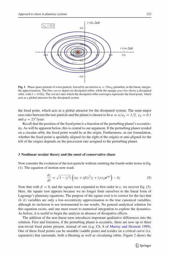
Figure 1 illustrates a phase space portrait of un-dissipated, as well as damped motion of atest-particle, perturbed by an exterior, m = 15m⊕ planet, orbiting a Sun-like (M = 1M�)

star. Variables are plotted such that the radial distance depicts the eccentricity of the test-parti-cle, while the polar angle represents the angle between the apsidal lines of the particle and theplanet. The blue curves depict un-dissipated orbits, while the opaque gray line shows a dissi-pated orbit, with δ = 0.02η. The red dot onto which the dissipated orbit converges represents

123


0.6 0.4 0.2 0.2 0.4 0.6

0.6

0.4

0.2

0.2

0.4

0.6

Fig. 1 Phase space portrait of a test particle, forced by an exterior m = 15m⊕ perturber, in the linear, integra-ble approximation. The blue curves depict un-dissipated orbits, while the opaque gray line shows a dissipatedorbit, with δ = 0.02η. The red dot onto which the dissipated orbit converges represents the fixed point, whichacts as a global attractor for the dissipated system

the fixed point, which acts as a global attractor for the dissipated system. The semi-majoraxes ratio between the test-particle and the planet is chosen to be α ≡ a/ap = 1/2, ep = 0.1and g = 23′′/year.

Recall that the position of the fixed point is a function of the perturbing planet’s eccentric-ity. As will be apparent below, this is central to our argument. If the perturbing planet residedon a circular orbit, the fixed point would be at the origin. Furthermore, in our formulation,whether the fixed point is apsidally aligned (to the right of the origin) or anti-aligned (to theleft of the origin) depends on the precession rate assigned to the perturbing planet.

3 Nonlinear secular theory and the onset of conservative chaos

Now consider the evolution of the test-particle without omitting the fourth-order terms in Eq.(1). The equation of motion now reads

dz

dt=

√1 − |z2|

(iηz + iβ|z2|z + iγ epeigt

)− δz (5)

Note that with β = 0, and the square root expanded to first order in e, we recover Eq. (3).Here, the square root appears because we no longer limit ourselves to the linear form ofLagrange’s planetary equations. The purpose of the square root is to correct for the fact that(h, k) variables are only a low-eccentricity approximation to the true canonical variables,although its inclusion is not instrumental to our results. No general analytical solution forthis equation exists, and one must resort to numerical integration to explore the dynamics.As before, it is useful to begin the analysis in absence of dissipative effects.

The addition of the non-linear term introduces important qualitative differences into thesolution. First and foremost, if the perturbing planet is eccentric, there are now up to threenon-trivial fixed points present, instead of one (e.g. Ch. 8 of Murray and Dermott 1999).One of these fixed points can be unstable (saddle point) and resides on a critical curve (i.e.separatrix) that surrounds, both a librating as well as circulating orbits. Figure 2 shows the

123


0.6

(a)

(c)

(e)

(b)

(d)

(f)

0.4 0.2 0.2 0.4 0.6

0.6

0.4

0.2

0.2

0.4

0.6

0.6 0.40.4 0.20.2 0.20.2 0.40.40.4 0.6

0.6

0.40.4

0.20.2

0.20.2

0.40.4

0.6

0.6 0.4 0.2 0.2 0.4 0.6

0.6

0.4

0.2

0.2

0.4

0.6

0.20.2 0.2

0.20.2 0.20.2

0.6 0.4 0.2 0.2 0.4 0.6

0.6

0.4

0.2

0.2

0.4

0.6

0.6 0.4 0.2 0.2 0.4 0.6

0.6

0.4

0.2

0.2

0.4

0.6

0.20.20.2

0.6 0.4 0.2 0.2 0.4 0.6

0.6

0.4

0.2

0.2

0.4

0.6

0.20.20.2

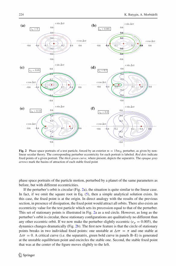
Fig. 2 Phase space portraits of a test particle, forced by an exterior m = 15m⊕ perturber, as given by non-linear secular theory. The corresponding perturber eccentricity for each portrait is labeled. Red dots indicatefixed points of a given portrait. The thick green curve, where present, depicts the separatrix. The opaque grayarrows mark the basins of attraction of each stable fixed point

phase space portraits of the particle motion, perturbed by a planet of the same parameters asbefore, but with different eccentricities.

If the perturber’s orbit is circular (Fig. 2a), the situation is quite similar to the linear case.In fact, if we omit the square root in Eq. (5), then a simple analytical solution exists. Inthis case, the fixed point is at the origin. In direct analogy with the results of the previoussection, in presence of dissipation, the fixed point would attract all orbits. There also exists aneccentricity value for the test particle which sets its precession equal to that of the perturber.This set of stationary points is illustrated in Fig. 2a as a red circle. However, as long as theperturber’s orbit is circular, these stationary configurations are qualitatively no different thanany other eccentric orbit. If we now make the perturber slightly eccentric (ep = 0.005), thedynamics changes dramatically (Fig. 2b). The first new feature is that the circle of stationarypoints breaks in two individual fixed points: one unstable at �� = π and one stable at�� = 0. A critical curve (i.e. the separatrix, green bold curve in panels B–E) is generatedat the unstable equilibrium point and encircles the stable one. Second, the stable fixed pointthat was at the center of the figure moves slightly to the left.

123


The appearance of new fixed points has ramifications for dissipative dynamics. As in thelinear example, if dissipation (assumed to be finite but much too small to noticeably modifythe dynamical portrait, i.e. lim δ → 0) were to be introduced, both of the stable fixed pointswould act as attractors, with their respective basins of attraction (shown as gray arrows inFig. 2) separated by the critical curve. The stability of fixed points that do not lie on thecritical curve, can be understood in the following qualitative manner. Consider a small libra-tion cycle, centered on one of the fixed points. The cycle’s intersections with the x-axis areplaced symmetrically, relative to the fixed point. The role of dissipation at the higher eccen-tricity intersection is to decrease the radius of libration, while that at the lower eccentricityintersection is to increase the radius of libration. Of the two antagonist effects, the first wins,because e ∝ e. Thus, the fixed points centered on libration cycles are stable foci.

As the eccentricity of the perturber is increased further to ep = 0.05 (Fig. 2c) and thento ep = 0.1 (Fig. 2d) the phase-space area engulfed by the inner branch of the separatrix(i.e. orbits centered around the stable anti-aligned fixed point) shrinks. Simultaneously, thephase-space area occupied by orbits that are librating around the aligned fixed point grows.When the perturber eccentricity reaches ep = 0.12, the apsidally anti-aligned fixed pointscollapse onto a single, unstable fixed point (Fig. 2e). This implies that if dissipation was to beincreased, no apsidally anti-aligned attractor would exist. If the eccentricity of the perturberis enhanced beyond ep > 0.12, the anti-aligned fixed point disappears completely from theportrait (Fig. 2d).

In both “end-member” scenarios we considered (ep = 0 and ep = 0.2), in presence ofdissipation, only a single attractor would exist. However, the attractors in these two casesarise from different fixed points (i.e. one can not be transformed into another by a change inep), centered around different branches of the separatrix. Recall that the sole fixed point thatwas present in the ep = 0 case, disappeared, when ep = 0.12. Similarly, The fixed point thatis present in the ep = 0.2 portrait is not present when the perturber’s orbit is circular. Thishas important implications for the motion of the particle when eccentricity of the perturberis not maintained at a constant value.

Consider a scenario where no dissipation is applied, but the eccentricity of the perturberis varied adiabatically between ep = 0 and ep = 0.2. Here, “adiabatically” means that theoscillation period of the perturber’s eccentricity greatly exceeds the apsidal circulation/libra-tion period of the test-particle. Regardless of the particle’s starting condition, its orbit willeventually encounter the separatrix. Since the separatrix is an orbit with an infinite preriod, itscrossing necessarily leads to chaotic motion (Bruhwiler and Cary 1989). In fact the situationis analogous to the motion of an amplitude-modulated pendulum. It has been shown that thechaotic region of such a system occupies the phase-space area that is swept by the separatrix(Henrard and Henrard 1991; Henrard and Morbidelli 1993). As a result, by ensuring that theeccentricity of the perturber reaches zero and extends above ep = 0.12 at every oscillation,we enforce the entire phase-space within e � 0.6 to be swept by the critical curve, causingall test-particles within this e-limit to become chaotic.

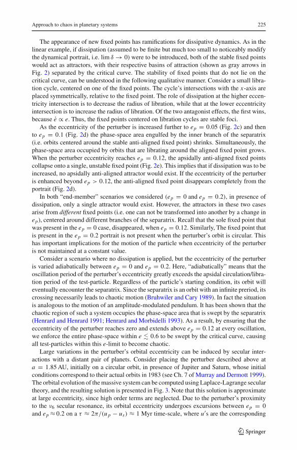
Large variations in the perturber’s orbital eccentricity can be induced by secular inter-actions with a distant pair of planets. Consider placing the perturber described above ata = 1.85 AU, initially on a circular orbit, in presence of Jupiter and Saturn, whose initialconditions correspond to their actual orbits in 1983 (see Ch. 7 of Murray and Dermott 1999).The orbital evolution of the massive system can be computed using Laplace-Lagrange seculartheory, and the resulting solution is presented in Fig. 3. Note that this solution is approximateat large eccentricity, since high order terms are neglected. Due to the perturber’s proximityto the ν6 secular resonance, its orbital eccentricity undergoes excursions between ep = 0and ep ≈ 0.2 on a τ ≈ 2π/(up − us) ≈ 1 Myr time-scale, where u′s are the corresponding

123


1 106 2 106 3 106 4 106

0.05

0.10

0.15

0.20

Fig. 3 Laplace–Lagrange secular solution of Jupiter, Saturn, and a m = 15m⊕ perturber at a = 1.85 AU. Theblack and red lines, which never go above e = 0.1 show the eccentricities of Jupiter and Saturn respectively.The blue and black curves, which attain high eccentricity, represent the exact Laplace–Lagrange solution andthe approximate solution, given by Eq. (6) for the perturber’s eccentricity

eigen-frequencies of the perturbation matrix and s refers to Saturn. Furthermore, the perturb-er’s longitude of perihelion in this solution precesses at a nearly constant rate of g = 23′′/year.For our purposes we approximate the variation in the perturber’s eccentricity as

ep ≈ 0.2

∣∣∣∣sin

(up − us

2

)t

∣∣∣∣ (6)

Addition of Jupiter and Saturn to the system does not significantly modify the evolution ofthe test-particle because of the substantial orbital separation between them (αj ∼ 0.2 and αs

∼ 0.1). In fact, evaluation of the corresponding constants η, β and γ shows that the particle’sinteractions with Saturn can be neglected all together, as they only contribute at the ∼ 1%level, while for Jupiter, it suffices to account only for the additional apsidal precession, towhich it contributes at the ∼ 30% level, compared to the effect of the considered planet(15m⊕). Quantitatively, this corresponds to an enhancement of the coefficients η and β, butnot γ . As stated in the Appendix, where the expressions for the constants are given, wehave been implicitly retaining the apsidal contribution due to Jupiter since the beginning ofthe paper, for consistency of the phase-space portraits. The difference in longitude of peri-helia between the test-particle and Jupiter forms a comparatively fast angle, and thus canbe averaged out. Consequently, we avoid its introduction into the Hamiltonian. This is fur-ther warranted, as the magnitude of the interaction term between Jupiter and the test-particle(i.e. γj ) is about an order of magnitude smaller than that of the test-particle and the m = 15m⊕perturber.1

Since the introduction of the variation of the perturber’s eccentricity, we are now facedwith a one-and-a-half degrees of freedom Hamiltonian. The dynamics of such a system isbest visualized by using a Poincarè surface of section. As in the phase-space portraits above,on a Poincarè surface of section, a periodic orbit will appear as a point, or a finite sequenceof points. A quasi-periodic orbit will appear as a curve that closes upon itself, while a chaotic

1 We could have generated an identical chaotic region by introducing another perturber that precesses slightlyslower, and tuning its parameters, such that the interaction coefficients in the Hamiltonian, γ are equal (seeSidlichovsky 1990, Lithwick and Wu 2010). Such a system would constitute a frequency-modulated pendulumrather than an amplitude-modulated one.

123


0.6 0.4 0.2 0.2 0.4 0.6

0.6

0.4

0.2

0.2

0.4

0.6

-0.75

0.75

0.75-0.75

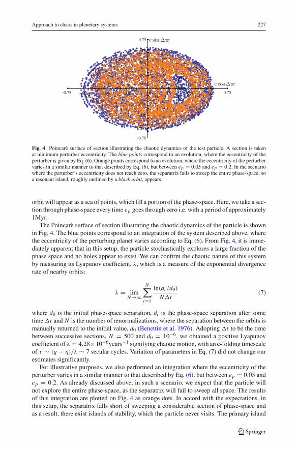
Fig. 4 Poincarè surface of section illustrating the chaotic dynamics of the test particle. A section is takenat minimum perturber eccentricity. The blue points correspond to an evolution, where the eccentricity of theperturber is given by Eq. (6). Orange points correspond to an evolution, where the eccentricity of the perturbervaries in a similar manner to that described by Eq. (6), but between ep = 0.05 and ep = 0.2. In the scenariowhere the perturber’s eccentricity does not reach zero, the separatrix fails to sweep the entire phase-space, soa resonant island, roughly outlined by a black orbit, appears

orbit will appear as a sea of points, which fill a portion of the phase-space. Here, we take a sec-tion through phase-space every time ep goes through zero i.e. with a period of approximately1Myr.

The Poincarè surface of section illustrating the chaotic dynamics of the particle is shownin Fig. 4. The blue points correspond to an integration of the system described above, wherethe eccentricity of the perturbing planet varies according to Eq. (6). From Fig. 4, it is imme-diately apparent that in this setup, the particle stochastically explores a large fraction of thephase space and no holes appear to exist. We can confirm the chaotic nature of this systemby measuring its Lyapunov coefficient, λ, which is a measure of the exponential divergencerate of nearby orbits:

λ = limN→∞

N∑i=1

ln(di/d0)

N�t(7)

where d0 is the initial phase-space separation, di is the phase-space separation after sometime �t and N is the number of renormalizations, where the separation between the orbits ismanually returned to the initial value, d0 (Benettin et al. 1976). Adopting �t to be the timebetween successive sections, N = 500 and d0 = 10−6, we obtained a positive Lyapunovcoefficient of λ = 4.28×10−6years−1 signifying chaotic motion, with an e-folding timescaleof τ ∼ (g − η)/λ ∼ 7 secular cycles. Variation of parameters in Eq. (7) did not change ourestimates significantly.

For illustrative purposes, we also performed an integration where the eccentricity of theperturber varies in a similar manner to that described by Eq. (6), but between ep = 0.05 andep = 0.2. As already discussed above, in such a scenario, we expect that the particle willnot explore the entire phase-space, as the separatrix will fail to sweep all space. The resultsof this integration are plotted on Fig. 4 as orange dots. In accord with the expectations, inthis setup, the separatrix falls short of sweeping a considerable section of phase-space andas a result, there exist islands of stability, which the particle never visits. The primary island

123


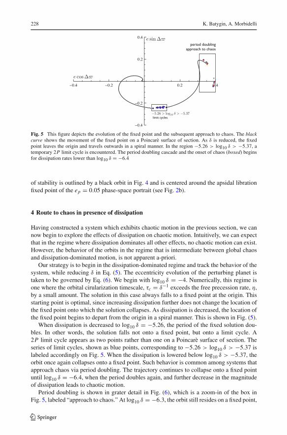
Fig. 5 This figure depicts the evolution of the fixed point and the subsequent approach to chaos. The blackcurve shows the movement of the fixed point on a Poincarè surface of section. As δ is reduced, the fixedpoint leaves the origin and travels outwards in a spiral manner. In the region −5.26 > log10 δ > −5.37, atemporary 2P limit cycle is encountered. The period doubling cascade and the onset of chaos (boxed) beginsfor dissipation rates lower than log10 δ = −6.4

of stability is outlined by a black orbit in Fig. 4 and is centered around the apsidal librationfixed point of the ep = 0.05 phase-space portrait (see Fig. 2b).

4 Route to chaos in presence of dissipation

Having constructed a system which exhibits chaotic motion in the previous section, we cannow begin to explore the effects of dissipation on chaotic motion. Intuitively, we can expectthat in the regime where dissipation dominates all other effects, no chaotic motion can exist.However, the behavior of the orbits in the regime that is intermediate between global chaosand dissipation-dominated motion, is not apparent a-priori.

Our strategy is to begin in the dissipation-dominated regime and track the behavior of thesystem, while reducing δ in Eq. (5). The eccentricity evolution of the perturbing planet istaken to be governed by Eq. (6). We begin with log10 δ = −4. Numerically, this regime isone where the orbital cirularization timescale, τc = δ−1 exceeds the free precession rate, η,by a small amount. The solution in this case always falls to a fixed point at the origin. Thisstarting point is optimal, since increasing dissipation further does not change the location ofthe fixed point onto which the solution collapses. As dissipation is decreased, the location ofthe fixed point begins to depart from the origin in a spiral manner. This is shown in Fig. (5).

When dissipation is decreased to log10 δ = −5.26, the period of the fixed solution dou-bles. In other words, the solution falls not onto a fixed point, but onto a limit cycle. A2P limit cycle appears as two points rather than one on a Poincarè surface of section. Theseries of limit cycles, shown as blue points, corresponding to −5.26 > log10 δ > −5.37 islabeled accordingly on Fig. 5. When the dissipation is lowered below log10 δ > −5.37, theorbit once again collapses onto a fixed point. Such behavior is common among systems thatapproach chaos via period doubling. The trajectory continues to collapse onto a fixed pointuntil log10 δ = −6.4, when the period doubles again, and further decrease in the magnitudeof dissipation leads to chaotic motion.

Period doubling is shown in grater detail in Fig. (6), which is a zoom-in of the box inFig. 5, labeled “approach to chaos.” At log10 δ = −6.3, the orbit still resides on a fixed point,

123


0.32 0.34 0.36 0.38 0.400.10

0.05

0.00

0.05

0.10

0.15

0.20

0.25

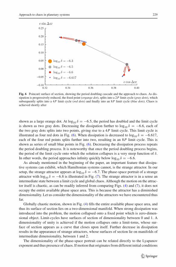
Fig. 6 Poincarè surface of section, showing the period doubling cascade and the approach to chaos. As dis-sipation is progressively reduced, the fixed point (organge dot), splits into a 2P limit cycle (gray dots), whichsubsequently splits into a 4P limit cycle (red dots) and finally into an 8P limit cycle (blue dots). Chaos isachieved shortly after

shown as a large orange dot. At log10 δ = −6.5, the period has doubled and the limit cycleis shown as two gray dots. Decreasing the dissipation further to log10 δ = −6.6, each ofthe two gray dots splits into two points, giving rise to a 4P limit cycle. This limit cycle isillustrated as four red dots in Fig. (6). When dissipation is decreased to log10 δ = −6.617,each of the four red points splits further into two, resulting in an 8P limit cycle. This isshown as series of small blue points in Fig. (6). Decreasing the dissipation process repeatsthe period doubling process. It is noteworthy that once the period doubling process begins,the period of the limit cycle onto which the solution collapses is a very steep function of δ.In other words, the period approaches infinity quickly below log10 δ = −6.6.

As already mentioned in the beginning of the paper, an important feature that dissipa-tive systems can exhibit, which Hamiltonian systems cannot, is the strange attractor. In oursetup, the strange attractor appears at log10 δ = −6.7. The phase-space portrait of a strangeattractor with log10 δ = −6.8 is illustrated in Fig. (7). The strange attractor is in a sense anintermediate state between a limit cycle and global chaos. Although the motion on the attrac-tor itself is chaotic, as can be readily inferred from comparing Figs. (4) and (7), it does notoccupy the entire available phase space area. This is because the attractor has a diminisheddimensionality. Let us consider the dimensionality of the attractors we have encountered thusfar.

Globally chaotic motion, shown in Fig. (4) fills the entire available phase space area, andthus its surface of section lies on a two-dimensional manifold. When strong dissipation wasintroduced into the problem, the motion collapsed onto a fixed point which is zero-dimen-sional object. Limit-cycles have surfaces of section of dimensionality between 0 and 1. Adimensionality of unity is achieved if the motion collapses onto a limit-torus, whose sur-face of section appears as a curve that closes upon itself. Further decrease in dissipationresults in the appearance of strange attractors, whose surfaces of section lie on manifolds ofintermediate dimensionality, between 1 and 2.

The dimensionality of the phase-space portrait can be related directly to the Lyapunovexponent and thus presence of chaos. If motion that originates from different initial conditions

123


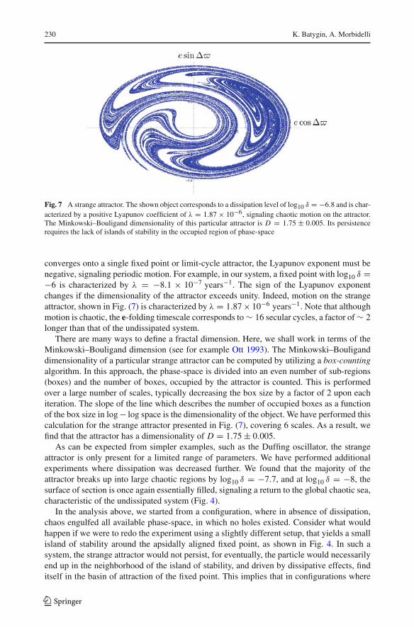
Fig. 7 A strange attractor. The shown object corresponds to a dissipation level of log10 δ = −6.8 and is char-acterized by a positive Lyapunov coefficient of λ = 1.87 × 10−6, signaling chaotic motion on the attractor.The Minkowski–Bouligand dimensionality of this particular attractor is D = 1.75 ± 0.005. Its persistencerequires the lack of islands of stability in the occupied region of phase-space

converges onto a single fixed point or limit-cycle attractor, the Lyapunov exponent must benegative, signaling periodic motion. For example, in our system, a fixed point with log10 δ =−6 is characterized by λ = −8.1 × 10−7 years−1. The sign of the Lyapunov exponentchanges if the dimensionality of the attractor exceeds unity. Indeed, motion on the strangeattractor, shown in Fig. (7) is characterized by λ = 1.87 × 10−6 years−1. Note that althoughmotion is chaotic, the e-folding timescale corresponds to ∼ 16 secular cycles, a factor of ∼ 2longer than that of the undissipated system.

There are many ways to define a fractal dimension. Here, we shall work in terms of theMinkowski–Bouligand dimension (see for example Ott 1993). The Minkowski–Bouliganddimensionality of a particular strange attractor can be computed by utilizing a box-countingalgorithm. In this approach, the phase-space is divided into an even number of sub-regions(boxes) and the number of boxes, occupied by the attractor is counted. This is performedover a large number of scales, typically decreasing the box size by a factor of 2 upon eachiteration. The slope of the line which describes the number of occupied boxes as a functionof the box size in log − log space is the dimensionality of the object. We have performed thiscalculation for the strange attractor presented in Fig. (7), covering 6 scales. As a result, wefind that the attractor has a dimensionality of D = 1.75 ± 0.005.

As can be expected from simpler examples, such as the Duffing oscillator, the strangeattractor is only present for a limited range of parameters. We have performed additionalexperiments where dissipation was decreased further. We found that the majority of theattractor breaks up into large chaotic regions by log10 δ = −7.7, and at log10 δ = −8, thesurface of section is once again essentially filled, signaling a return to the global chaotic sea,characteristic of the undissipated system (Fig. 4).

In the analysis above, we started from a configuration, where in absence of dissipation,chaos engulfed all available phase-space, in which no holes existed. Consider what wouldhappen if we were to redo the experiment using a slightly different setup, that yields a smallisland of stability around the apsidally aligned fixed point, as shown in Fig. 4. In such asystem, the strange attractor would not persist, for eventually, the particle would necessarilyend up in the neighborhood of the island of stability, and driven by dissipative effects, finditself in the basin of attraction of the fixed point. This implies that in configurations where

123


chaos is not global, the presence of dissipation tends to guide the constituents towards regularorbits, with the degree of dissipation directly dictating the time-scale needed for the system’sarrival to a quasi-periodic state.

5 Discussion

In this paper, we investigate the onset of chaotic motion in planetary systems, where dis-sipative effects play an important role. Using a semi-analytical perturbation approach, wehave shown that planetary chaos appears through a period doubling cascade. We have furtherdemonstrated that strange attractors can exist in the context of a planetary problem under thecondition of global chaos in absence of dissipation.

It is important to consider the astrophysical significance of this process, beyond purelyacademic interest. As already mentioned in the beginning of the manuscript, one can expectthe period doubling cascade to occur during early epochs of a planetary system’s dynamicalevolution, as the evaporation of the birth nebula leads to a gradual decrease in dissipation.As a result, the work presented here describes how the dynamical portrait of a system mayevolve shortly after formation, when gas is gradually taken away. Note that the dissipationtimescale, corresponding to the strange attractor, is typical of a late-stage proto-planetarydisk (i.e. τcirc ∼ 106years) (Lee and Peale 2002). In other words, the example configurationdescribed here may correspond to a planetary system where the planets are already massiveenough to have essentially decoupled from the gas, and are forcing a small planetesimal,which still feels considerable drag.

Other forms of dissipation, such as tides, are abundantly present in the planetary context,and are of special importance for hot exoplanets. This is further relevant, since understand-ing the dynamics of multiple close-in planets is becoming increasingly important, as theirnumbers in the observed aggregate grow. Particular interest is exhibited towards orbital con-figurations that converge to a fixed point, since a stationary system is required for obtainingan estimate for the Love number, k2, of extra-solar gas giants (Batygin et al. 2009). Althoughlinear theory predicts that a dissipated system’s arrival to a stationary configuration is onlya matter or time (i.e. tidal Q) (Goldreich and Soter 1966), non-linear theory presented here,suggests that one should exercise caution, as a fixed point is not always the end-state.

The same problem can also be turned around. We have shown here that limit cycles residein limited parameter regimes. Thus, an observed system, whose orbital evolution follows alimit-cycle, can be used to place desperately needed constraints on the tidal quality factor,which remains among the most unconstrained parameters in planetary science and whosephysical origin is an area of ongoing research (Wu 2005).

For close-in planets, the effect of general relativity and tidal precession plays in favorof approach to the fixed point, rather than any other attractors. This is because it enhancesthe coefficients η and β, but not γ , in the Hamiltonian. Since the orbital precession of aputative external perturber will generally be comparatively slow, the enhanced precession ofclose-in planets will tend to de-tune any resonance. As the relative amplitude of the externalperturbations is diminished, the dynamics approaches the ep = 0 phase-space portrait seenin Fig. 2a. Naturally, this will also lead to stabilization of the orbits. It is noteworthy thatsuch an effect is also at play in the Solar System, as additional precession from GR places thefree precession of Mercury further from the ν5 secular resonance, diminishing its chances ofejection (Batygin and Laughlin 2008; Laskar and Gastineau 2009).

Finally, it is worthwhile to consider the limitations of the presented model. Indeed, we haveapproached the problem by utilizing a classical perturbation theory, where only a few relevant

123


terms are retained in the disturbing function. As already mentioned above, this approach wasnecessary for the exploration of parameter space, as the efficiency offered by conventionaldirect integration is not sufficient. Although the approach we take here breaks down at higheccentricities, in the Solar System, it has been successful in capturing the important physicalprocesses that govern chaotic motion (Sidlichovsky 1990). The recent work of Lithwick andWu (2010) has further confirmed this to be true in the case of Mercury’s orbit. Thus, we expectthat inclusion of the full disturbing function will only modify our findings on a quantitativelevel. However, future numerical confirmation and re-eavluation of the work done here willsurely be a fruitful venture, especially if performed in the context of a particular observedsystem.

Acknowledgments We thank K. Tsiganis for numerous useful discussions and Oded Aharonson for carefullyreviewing the manuscript. Additionally, we thank the anonymous referees four useful suggestions.

Appendix: Coefficients of the Hamiltonian

In this work, we choose to write the coefficients, such that they appear in the equationsof motion without pre-factors. The notation used here is identical to that of Murray andDermott (1999), i.e. b denotes a Laplace coefficient, α is the semi-major axis ratio, andD ≡ ∂/∂α. Throughout the paper, we account for the induced precession that arises fromthe m = 15m⊕, αp = 1/2 perturber as well as Jupiter, with αJ = 0.178, but not Saturn.Evaluation of the formulae below shows that Saturn’s effect is negligible. The eccentricityforcing, taken into account is solely due to the m = 15m⊕ perturber. The resulting formulaeread:

η = n

4

(mp

M

a

ap

(2αpD + α2

pD2)

b(0)12

(αp) + mJ

M

a

aJ

(2αJD + α2

JD2) b(0)12

(αJ )

)(1)

β = n

32

(mp

M

a

ap

(4α3

pD3 + α4pD4

)b

(0)12

(αp) + mJ

M

a

aJ

(4α3

JD3 + α4JD4) b

(0)12

(αJ )

)(2)

γ = n

4

mp

M

a

ap

(2 − 2αpD − α2D2) b

(1)12

(αp) (3)

The first and the second terms in η and β arise from the m = 15m⊕ perturber and Jupiterrespectively. All terms in γ correspond to the m = 15m⊕ perturber.

References

Albers, D.J., Sprott, J.C.: Routes to chaos in high-dimensional dynamical systems: a qualitative numericalstudy. Phys. D Nonlinear Phenom. 223, 194–207 (2006)

Batygin, K., Bodenheimer, P., Laughlin, G.: Determination of the interior structure of transiting planets inmultiple-planet systems. Astrophys. J. 704, L49–L53 (2009)

Batygin, K., Laughlin, G.: On the dynamical stability of the solar system. Astrophys. J. 683, 1207–1216 (2008)Batygin, K., Laughlin, G., Meschiari, S., Rivera, E., Vogt, S., Butler, P.: A quasi-stationary solution to Gliese

436b’s eccentricity. Astrophys. J. 699, 23–30 (2009)Batygin, K., Laughlin, G.: Resolving the sin(I) degeneracy in low-mass multi-planet systems. Astrophys. J. 730,

95 (2011)Beauge, C., Ferraz-Mello, S.: Resonance trapping in the primordial solar nebula—the case of a Stokes drag

dissipation. Icarus 103, 301–318 (1993)Benettin, G., Galgani, L., Strelcyn, J.-M.: Kolmogorov entropy and numerical experiments. Phys. Rev. A 14,

2338–2345 (1976)

123


Bruhwiler, D.L., Cary, J.R.: Diffusion of particles in a slowly modulated wave. Phys. D Nonlinear Phenom.40, 265–282 (1989)

Chirikov, B.V.: A universal instability of many-dimensional oscillator systems. Phys. Rep. 52, 263–379 (1979)Goldreich, P., Soter, S.: Q in the solar system. Icarus 5, 375–389 (1966)Gonczi, R., Froeschle, C., Froeschle, C.: Poynting–Robertson drag and orbital resonance. Icarus 51, 633–654

(1982)Henrard, J., Henrard, M.: Slow crossing of a stochastic layer. Phys. D Nonlinear Phenom. 54, 135–146 (1991)Henrard, J., Lemaitre, A.: A second fundamental model for resonance. Celest. Mech. 30, 197–218 (1983)Henrard, J., Morbidelli, A.: Slow crossing of a stochastic layer. Phys. D Nonlinear Phenom. 68, 187–200 (1993)Laskar, J.: A numerical experiment on the chaotic behaviour of the solar system. Nature 338, 237 (1989)Laskar, J.: Large-scale chaos in the solar system. Astron. Astrophys. 287, L9–L12 (1994)Laskar, J.: Large scale chaos and marginal stability in the solar system. Celest. Mech. Dyn. Astron. 64,

115–162 (1996)Laskar, J., Gastineau, M.: Existence of collisional trajectories of mercury, mars and venus with the

earth. Nature 459, 817–819 (2009)Lee, M.H., Peale, S.J.: Dynamics and origin of the 2:1 orbital resonances of the GJ 876 planets. Astrophys.

J. 567, 596–609 (2002)Lithwick, Y., Wu, Y.: Theory of Secular Chaos and Mercury’s Orbit. ArXiv e-prints arXiv:1012.3706 (2010)Lovis, C. et al.: The HARPS search for southern extra-solar planets. XXVIII. Up to seven planets orbiting HD

10180: probing the architecture of low-mass planetary systems. Astron. Astrophys. 528, A112 (2011)Mardling, R.A.: Long-term tidal evolution of short-period planets with companions. Monthly Notices Roy.

Astron. Soc. 382, 1768–1790 (2007)Morbidelli, A.: Modern Celestial Mechanics: Aspects of Solar System Dynamic. Taylor Francis, London,

ISBN 0415279399 (2002)Murray, C.D., Dermott, S.F.: Solar System Dynamics. Cambridge (1999)Murray, N., Holman, M.: The origin of chaos in the outer solar system. Science 283, 1877 (1999)Ott, E.: Chaos in Dynamical Systems. Cambridge University Press, Cambridge, pp. c1993 (1993)Sidlichovsky, M.: The existence of a chaotic region due to the overlap of secular resonances nu5 and nu6.

Celest. Mech. Dyn. Astron. 49, 177–196 (1990)Wisdom, J.: The resonance overlap criterion and the onset of stochastic behavior in the restricted three-body

problem. Astron. J. 85, 1122–1133 (1980)Wu, Y.: Origin of tidal dissipation in jupiter. II. The value of Q. Astrophys. J. 635, 688–710 (2005)Wu, Y., Goldreich, P.: Tidal evolution of the planetary system around HD 83443. Astrophys. J. 564,

1024–1027 (2002)

123

Documents

Onset of secular chaos in planetary systems: period