FACULDADE DE ENGENHARIA DA UNIVERSIDADE DO PORTO

Online model estimation for predictivecontrol of air conditioners in buildings

Bruno Miguel Tulha Moreira

Mestrado Integrado em Engenharia Eletrotécnica e de Computadores

Supervisor: João Peças Lopes

Second Supervisor: José Pedro Iria

January 22, 2018

c© Bruno Tulha, 2018

Abstract

The foreseen deployment of advanced building automation technologies promises to turn passiveconsumers into active prosumers. Building automation technologies includes communication,monitoring and control functionalities. These technologies can render great benefits to the powersystems by increasing the flexibility of the demand side. Demand flexibility is widely acknowl-edged as a solution to increase the integration of renewable energy sources, improve the operationof the transmission and distribution networks, and enhance the economic effectiveness of electric-ity markets.

Likewise, in order to overcome the variability and uncertainty that renewable energies bringto the system, it is necessary to control energy on the demand side, i.e. on the consumer side. Thesolutions go through the management and control of energy used in buildings and the optimizationof the energy equipment that are part of it. These solutions include a number of features, such asdevice monitoring, enabling a variety of new services to users.

Thus, in order to develop a methodology to control and monitor the loads of a building, initiallya bibliographic review is performed, where the problem is analysed in more detail. Afterwards,various models and information necessary to address this problem are explored, as well as possiblesolutions and methods of other authors.

Later, in this dissertation a model capable of determining the parameters of a given room ispresented, predicting its thermal behaviour for a given day, every 15 minutes for 24 hours, basedon online data. For the determination of these parameters a grey box model is proposed using theleast-squares method. Several models and results are presented and analysed to show in detail thework that has been developed.

After determining the parameters that model the thermal behaviour of the room, it is demon-strated how the determination of these parameters plays an important role in the control and mon-itoring of an energy resource. Afterwards, an optimization model of an air conditioner and itsimplementation strategy is presented. The results of the use of the air conditioning and its costsare demonstrated, proving that is possible to minimize costs and comply with the comfort require-ments established by the user.

i

ii

Resumo

O crescente incentivo ao avanço tecnológico inerente às redes inteligentes (smart grids) e edifíciosinteligentes (smart buildings) cumpre um papel essencial na forma de atuar dos consumidores,contribuindo para que estes passem a desempenhar um papel ativo na rede em vez de serem merosconsumidores passivos. As tecnologias de automação dos edifícios inteligentes pretendem incluirfuncionalidades de comunicação, monitorização e controlo. Estas tecnologias podem oferecergrandes benefícios aos sistemas de energia, aumentando a flexibilidade do lado da procura. Aflexibilidade referente à procura é amplamente reconhecida como uma solução para aumentar aintegração de energias renováveis, reduzir os consumos energéticos, melhorar o funcionamentodas redes de transmissão e distribuição e aumentar a eficácia econômica dos mercados elétricos.

Do mesmo modo, para combater a variabilidade e incerteza que as energias renováveis trazemao sistema, torna-se necessário controlar a energia do lado da procura, ou seja, do lado do con-sumidor. As soluções passam pela gestão e controlo do uso da energia em edifícios e otimizaçãodos recursos energéticos que dele fazem parte. Essas soluções incluem um conjunto de funcional-idades, como o controlo e monitorização de dispositivos, possibilitando uma variedade de novosserviços aos utilizadores.

Assim, com o intuito de desenvolver uma metodologia para controlar e monitorizar as cargasde um edifício, inicialmente é realizada uma revisão bibliográfica, onde é analisado com maisdetalhe o problema exposto. De seguida são explorados vários modelos e informações necessáriaspara abordar este problema, bem como possíveis soluções e métodos de outros autores.

Posteriormente é apresentado nesta dissertação um modelo capaz de determinar os parâmetrosde uma determinada sala, prevendo o comportamento térmico da mesma para um determinado dia,de 15 em 15 minutos durante 24h, baseado em dados on-line. Para a determinação destes parâmet-ros é proposto um modelo “grey box” juntamente com uma minimização dos erros quadrados.Vários modelos e resultados são analisados para se compreender o que foi realizado.

Após a determinação dos parâmetros que modelizam o comportamento térmico da sala, édemonstrado como a determinação destes parâmetros cumpre um papel importante no controloe monitorização de um recurso energético. Assim, é apresentado um modelo de otimização deum ar condicionado e a respetiva estratégia de implementação. São demonstrados os resultadosda utilização do ar condicionado e respetivos custos, sendo percetível que é possível minimizarcustos e obedecer aos requisitos de conforto estabelecidos pelo utilizador.

iii

iv

Acknowledgments

First of all, I would like to thank my thesis supervisor Prof. Dr. João Peças Lopes for acceptingthis supervision and for all the discussions and cutting-edge ideas during this journey to steer andimprove this thesis. I also want to acknowledge my co-supervisor, José Iria, for his guidance,availability, advise and for his essential contribution on the work developed.

A special word goes to Dr. Joel Soares, for the opportunity of working in such an interestingfield, constant motivation and his willingness to lend a hand throughout this entire journey. A bigthank you.

An acknowledgment is also due to all the people who worked with me in INESC TEC. I’mvery grateful to have had the opportunity to work in the same space with all these fantastic people.In particular I would like to thank the useful insights and help from António Barbosa and also, Iwant to thank Ricardo Andrade for the help he gave me during the development of my work.

I would also like to thank all my friends for being part of this journey and making my daysalways special.

Finally, to my parents, the most important people ever, I want to express my deepest thanksfor all the help, love and support shown over the years. Thank you for all the teachings and for allthe strength you have always given me, which has helped me to grow and overcome all obstacles.No doubt the completion of this dissertation would not have been possible without you.

Thank you.

Bruno Miguel Tulha Moreira

v

vi

This thesis was developed under the framework of GREsBAS project (SmartGP/0003/2015) andSmartGuide project (SmartGP/0002/2015), which are financed by Fundação para a Ciência eTecnologia (FCT) under the framework of the ERA-Net Smart Grids Plus initiative.

Part of this work was also integrated with the project SAICTPAC/0004/2015-POCI-01-0145-FEDER-016434, funded by the ERDF – European Regional Development Fundthrough the Operational Programme for Competitiveness and Internationalisation - COMPETE2020 programme, and by National Funds through FCT.

“Strength does not come from physical capacity.It comes from an indomitable will.”

Mahatma Gandhi

vii

viii

Contents

1 Introduction 11.1 Motivation . . . . . . . . . . . . . . . . . . . . . . . . . . . . . . . . . . . . . . 11.2 Objectives . . . . . . . . . . . . . . . . . . . . . . . . . . . . . . . . . . . . . . 21.3 Thesis Organization . . . . . . . . . . . . . . . . . . . . . . . . . . . . . . . . . 3

2 State-of-the-Art 52.1 Smart Building . . . . . . . . . . . . . . . . . . . . . . . . . . . . . . . . . . . 52.2 Smart Grid . . . . . . . . . . . . . . . . . . . . . . . . . . . . . . . . . . . . . 62.3 Active Control of Loads . . . . . . . . . . . . . . . . . . . . . . . . . . . . . . 62.4 Control Strategies . . . . . . . . . . . . . . . . . . . . . . . . . . . . . . . . . . 82.5 Approaches to Thermal Modeling of Buildings . . . . . . . . . . . . . . . . . . 92.6 Modeling Approaches . . . . . . . . . . . . . . . . . . . . . . . . . . . . . . . . 92.7 Model Type . . . . . . . . . . . . . . . . . . . . . . . . . . . . . . . . . . . . . 10

2.7.1 White Box Model . . . . . . . . . . . . . . . . . . . . . . . . . . . . . . 112.7.2 Black Box Model . . . . . . . . . . . . . . . . . . . . . . . . . . . . . . 112.7.3 Grey Box Model . . . . . . . . . . . . . . . . . . . . . . . . . . . . . . 12

2.8 Load Modelling . . . . . . . . . . . . . . . . . . . . . . . . . . . . . . . . . . . 122.9 Parameter Estimation . . . . . . . . . . . . . . . . . . . . . . . . . . . . . . . . 15

3 Methodology 193.1 Models Used . . . . . . . . . . . . . . . . . . . . . . . . . . . . . . . . . . . . 20

3.1.1 Thermal Model . . . . . . . . . . . . . . . . . . . . . . . . . . . . . . . 203.1.2 HVAC Optimization Model . . . . . . . . . . . . . . . . . . . . . . . . 23

3.2 Strategy Used . . . . . . . . . . . . . . . . . . . . . . . . . . . . . . . . . . . . 24

4 Case Study and Analysis of Results 294.1 Case Study . . . . . . . . . . . . . . . . . . . . . . . . . . . . . . . . . . . . . 294.2 Analysis of Results . . . . . . . . . . . . . . . . . . . . . . . . . . . . . . . . . 34

4.2.1 Thermal Model . . . . . . . . . . . . . . . . . . . . . . . . . . . . . . . 344.2.2 HVAC Optimization . . . . . . . . . . . . . . . . . . . . . . . . . . . . 40

5 Conclusion, Main Achievements and Future Work 495.1 Conclusion and Main Achievements . . . . . . . . . . . . . . . . . . . . . . . . 495.2 Future Work . . . . . . . . . . . . . . . . . . . . . . . . . . . . . . . . . . . . . 50

References 53

A Tables of Thermal Model 59

ix

x CONTENTS

B Tables of AC Optimization 67

List of Figures

2.1 Comparison of the white box modeling approach (left) with the grey box mod-elling approach(centre) and the black box modeling approach (right) – adaptedfrom [33] . . . . . . . . . . . . . . . . . . . . . . . . . . . . . . . . . . . . . . 11

2.2 Example of an energy system and energy exchanges . . . . . . . . . . . . . . . . 132.3 Equivalent between RC electric circuit and AC thermal process – adapted from [43] 14

3.1 General Methodology of the work developed . . . . . . . . . . . . . . . . . . . 193.2 Model system and interactions between the end-user, EMS and smart appliances . 203.3 Representative model of strategy used in thermal model and optimization model . 243.4 System architecture of data collection . . . . . . . . . . . . . . . . . . . . . . . 26

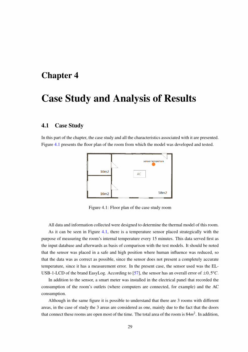
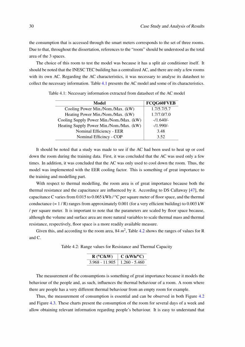
4.1 Floor plan of the case study room . . . . . . . . . . . . . . . . . . . . . . . . . . 294.2 Consumption every 15 minutes for each day of one week (from 6/11/2017 to

12/11/2017) . . . . . . . . . . . . . . . . . . . . . . . . . . . . . . . . . . . . . 314.3 Consumption every 15 minutes for each day of a week (from 30/10/2017 to 5/11/2017) 314.4 Radiation every 15 minutes for each day of a week (from 30/10/2017 to 05/11/2017) 334.5 Comparison between indoor and outdoor temperature for the day 30/10/2017 . . 334.6 Comparison between predictive temperature and real temperature for the case 1 . 354.7 Comparison between predictive temperature and real temperature for the case 2 . 364.8 Comparison between predictive temperature and real temperature for the case 3 . 374.9 Comparison between predictive temperature and real temperature for the case 4 . 384.10 Comparison between predictive temperature and real temperature for day 28/11/2017 394.11 Comparison between predictive temperature and real temperature for day 26/11/2017 394.12 Comparison between forecasted temperature and real temperature for day 24/10/2017 424.13 Comparison between predictive temperature with and without optimization for

case 1 . . . . . . . . . . . . . . . . . . . . . . . . . . . . . . . . . . . . . . . . 434.14 AC operation with and without optimization for case1. 1 when AC is On and 0

when AC is off . . . . . . . . . . . . . . . . . . . . . . . . . . . . . . . . . . . 434.15 Comparison between forecasted temperature with and without optimization for

case 2 . . . . . . . . . . . . . . . . . . . . . . . . . . . . . . . . . . . . . . . . 444.16 AC operation with and without optimization for case 2 . . . . . . . . . . . . . . 444.17 Comparison between forecasted temperature with and without optimization for

case 3 . . . . . . . . . . . . . . . . . . . . . . . . . . . . . . . . . . . . . . . . 454.18 AC operation with and without optimization for case 3 . . . . . . . . . . . . . . 454.19 Temperature with optimization for case 4 . . . . . . . . . . . . . . . . . . . . . 464.20 AC operation for case 4, heating and cooling . . . . . . . . . . . . . . . . . . . . 47

xi

xii LIST OF FIGURES

List of Tables

3.1 Variables and respective units . . . . . . . . . . . . . . . . . . . . . . . . . . . . 223.2 Heat gain from typical computer equipment and lamps . . . . . . . . . . . . . . 233.3 Representative of total heat gain by an adult person in moderately active office work 233.4 Symbol of input variables and outputs that we intend to determine . . . . . . . . 25

4.1 Necessary information extracted from datasheet of the AC model . . . . . . . . . 304.2 Range values for Resistance and Thermal Capacity . . . . . . . . . . . . . . . . 304.3 Maximum number of elements that produce heat in the room . . . . . . . . . . . 324.4 Total heat gain in kW by the elements mentioned in Table 4.3 . . . . . . . . . . . 324.5 Values of MAE for each of the days and value of MAE for one whole week . . . 394.6 Value of MAE for one whole week . . . . . . . . . . . . . . . . . . . . . . . . . 404.7 Tariffs values for each time period . . . . . . . . . . . . . . . . . . . . . . . . . 414.8 Optinal weekly cycle for MAT, AT and MT in Portugal . . . . . . . . . . . . . . 41

A.1 Parameters determined for 24h every 15 minutes, for the case 2 . . . . . . . . . . 59A.2 Parameters determined for 24h every 15 minutes, for the case 3 . . . . . . . . . . 60A.3 Parameters determined for 24h every 15 minutes, for the case 4 . . . . . . . . . . 62

B.1 AC power values with and without optimization for case 1 . . . . . . . . . . . . 67B.2 AC power values with and without optimization for case 2 . . . . . . . . . . . . 68B.3 AC power values with and without optimization for case 3 . . . . . . . . . . . . 69B.4 AC power values with optimization for case 4, heating and cooling . . . . . . . . 70

xiii

xiv LIST OF TABLES

Abbreviation and Symbols

List of Abbreviations

DG Distributed GenerationEV Electric VehiclesHVAC Heating, Ventilation and Air ConditioningAC Air ConditioningSG Smart GridSB Smart BuildingBEMS Building Energy Management SystemHEMS Home Energy Management SystemEMS Energy Management SystemMPC Model Predictive ControlEMPC Economic Model Predictive ControlPBLM Physically Based Load Models

List of Symbols

Parameters∆t Time intervalR ResistanceC Thermal CapacitanceCOP Coeficient Of PerformanceEER Energy Efficiency RatioPmax Maximum electric powerθmin Minimum temperature limitθmin Maximum temperature limit

Variablesθreal,t Real temperature at time tθpred,t Predicted temperature at time tθt+1 Temperature of the next time intervalθt Temperature at time tθ 0

t Outdoor temperature at time tPt Electric power at time tConst Electric power consumption at time tRadt Power radiation at time twCt Weight of Consumption at time t for weekdaysw_fsC,t Weight of Consumption at time t for weekends

xv

xvi Abbreviation and Symbols

wRt Weight of Radiation at time t for weekdaysw_fsR,t Weight of Radiation at time t for weekendswEt External gains at time t for weekdaysw_fsE,t External gains at time t for weekendstarifft Price to be paid for the energy at time tPheating,t Electric AC heating power at time tPcooling,t Electric AC cooling power at time t

Chapter 1

Introduction

In this chapter, a brief overview of the main topics of the work is presented. Firstly, the motivation

for the thesis and the importance that it has in the context of smart grids and energy efficiency is

presented, followed by the proposed objectives. Finally, the structure of this thesis and its rationale

is described.

1.1 Motivation

Nowadays, there is a big concern about energy consumption and in a generalized way, the impor-

tance of electrical energy to our society has been growing, since electricity will be largely used in

order to allow the decarbonisation of economy and of the society. This requires finding innovative

ways and means to make energy supply as sustainable as possible.

Regarding the issue of energy consumption, buildings account for 20 to 40% of the energy

used in developed countries [1]. Buildings represent 40% of total consumption in the European

Union [2] and 37% in the United States [1].

This area of research is growing rapidly, as is the case in countries such as China or India,

where there is rapid growth in housing construction. In fact, there are more factors that lead to

increasing consumption. As an example, people increasingly seek to increase their comfort levels,

buildings are getting bigger, there are more quantities of household equipment and in addition

there is a marked increase with regard to the integration of electric vehicles.

Besides that, the underdeveloped countries are growing fast and, consequently, consuming

more energy. The more the quality of life increases the more energy is consumed and the more

emissions of CO2 are created leading to serious environmental problems.

Thus, to overcome to environmental problems and to combat emissions of greenhouse gases

in an effective way, the incentives and plans to support renewable energies should increase signifi-

cantly. The well-known European Union’s "20-20-20" plan, for instance, stipulates that emissions

of greenhouse gases should be reduced by 20% (taking into account 1990 values) and renewables

should present 20% of the energy consumption of the European Union by 2020 [3].

1

2 Introduction

In order to combat climate change and make a positive contribution to energy efficiency, the

concept of smart buildings is grasping increasing attention by policy makers. The incentive to

technological advancement as well as the current organizational structure implemented plays an

essential role in advancing this topic. This advance, which is taking its first steps, is aimed at

reducing consumption, while at the same time improving comfort levels.

Likewise, the increase on energy production based on renewable sources is seen as a solution

to achieve a significant reduction of CO2 emissions. Due to the high degree of uncertainty that

characterizes renewables, it is imperative to find solutions to tackle this issue. Thus, it is necessary

to develop advanced programming models using robust and predictive control models capable of

handling and modelling this uncertain behaviour.

In the current paradigm, buildings are seen as a simple consumer, however, there are more and

more resources that can have an active behaviour in the network, apart from the building electrical

devices’s or household appliances as is the case of Distributed Generation (DG) units, storage

systems and Electric Vehicles (EV).

By that, in view of this new concept, it becomes imperative to carry out the optimal manage-

ment of energy resources in a building.

In a building, lighting and air conditioning systems are mainly responsible for the highest

level of consumption. Heating, Ventilation, and Air Conditioning (HVAC) and lighting systems

account for about 40% and 15% of consumption [4], respectively. Thus, the great potential in the

management of energy resources will be mainly in the systems of air conditioning of buildings.

In conclusion, with the purpose to solve the aforementioned intentions, the objective is to

change customers’ normal use of electricity (consumption) through an optimal management of the

energy resources available, in order to increase the efficiency and sustainability of buildings, while

maximizing the penetration of renewable energy sources.

1.2 Objectives

The aim of this Master thesis is to develop mathematical models to exploit the net load flexibility

of buildings with the objective of minimizing energy costs. This includes the development of sim-

plified data-driven thermal models and decision aid tools to optimize the operation of distributed

energy resources (e.g. HVAC).

So, in this context, it is necessary to develop methods and models of parameter estimation to

later determine the best thermal model of the room and to be able to place these parameters in the

air conditioning model and optimize its operation. It should be noted that these parameters are

elements that we want to determine, such as thermal gains or losses as well as physical properties

from the room itself.

On top of that, the model should account for future disturbances by incorporating weather

predictions and others (such as thermal gains) in the optimization.

Regarding residential and corporate buildings, it is imperative to reduce their energy consump-

tion. Thus, it is important to know the thermal behaviour of buildings and evaluate their energy

1.3 Thesis Organization 3

consumption. For this, it is mandatory to formulate tailored models that can be used to perform

room temperature predictions and thus enhance overall energy performance. The proposed tools

will be developed within the framework of the European project GREsBAS and will be tested

through simulations with data gathered from a real demonstration site (INESC TEC building).

In conclusion, the objective is to develop an estimation and optimization thermal model for

corporate or residential buildings, which can be used to optimize air conditioning utilization and

minimize its energy consumption.

1.3 Thesis Organization

This thesis is composed by five chapters.

The current, and first one, serves as a general exposure of the motivation for this thesis as well

as the fundamental aims of this work.

The State of the Art is presented in the second chapter. In this chapter a brief review about

smart building, smart grids and active loads control is performed. Then, an overview about control

strategies carried out by other authors as well as approaches to thermal modelling are presented

followed by a description of the modelling approaches and the different types (white box, grey

box, and black box approach). Finally, the load modelling and the connection between this and

the parameters estimation is presented. An overview about different load modelling methods and

about different parameter estimation models by other authors is given.

Chapter 3 presents and describes the methodology and the strategy implemented to estimate

the parameters that describe the thermal behaviour of the room. In this chapter is also presented

the thermal model used and all the inputs and outputs that we want to determine as well as is

presented and described the optimization model of the AC.

In chapter 4, the case study and the prediction results are presented for the parameter esti-

mation and then for the AC optimization. The results of thermal behaviour predicted with the

estimation parameters are presented and a comparison with the real results can be compared. Re-

garding the model of AC optimization, the costs of using AC with and without optimization can

be seen and compared.

Finally, in chapter 5, the main conclusions and achievements will be explicitly depicted and

some suggestions about future work will be given.

4 Introduction

Chapter 2

State-of-the-Art

Parallel to the technological advance there is an increase in the penetration of renewable ener-

gies. In the future, this penetration is expected to continue to increase, particularly in the form of

microgeneration. So, it becomes imperative to manage these energy systems.

Thus, concepts such as Smart Grid (SG) and Smart Building (SB) represent solutions that

allow the management of energy resources through a communication network between all the

devices, allowing control, monitoring, increasing efficiency and sustainability of buildings and the

electricity grid.

2.1 Smart Building

Improving energy efficiency in buildings is a critical issue to reduce the CO2 footprint, i.e., the

greater the efficiency of a building, the lower the energy consumption and the CO2 emissions.

It is important to emphasize that the introduction of renewable energy sources in buildings has

a direct impact on the reduction of CO2 emission levels, because the consumption can be partially

fed locally, reducing the energy absorbed from the grid.

The concept of SB is therefore motivated by the need to improve energy efficiency, coupled

with the need to integrate renewable energy production units. Furthermore, SB is not only a

building with self-production, but also is a building with controllable loads (smart loads). These

loads can be actively controlled and managed by complex systems of optimization in order to

increase user comfort and reduce energy consumption.

Thus, the goal is to make buildings more energy efficient, providing higher comfort levels to

the users. In a SB the devices are manageable, and the coordination of the energy consumption is

carried out locally. This new concept is gaining ground and becoming more attractive and viable.

The idea is help the occupants of a building managing their resources from the perspective of cost,

comfort, safety and flexibility.

According to Bingnan Jiang and Yunsi Fei [5], a building to be considered intelligent must

contain intelligent control systems and a communication network. The control systems receive

and interpret the information collected through sensors, intelligently process this information and

5

6 State-of-the-Art

send the actions to the actuators. SB are integrated into an infrastructure capable of controlling

and managing the energy production of all its stakeholders, called Smart Grid (SG).

2.2 Smart Grid

A SG is designated as a smart and modern grid that allows monitoring and acting on the generation,

transmission, distribution and consumption of energy.

Heleno et al. [6, 7] defines SG as a vision of the electric grids of the future raised from the

interest in electricity market opportunities after the unbundling of the electricity sector as well

as in new services associated with distributed energy resources, such as distributed generation,

storage and the flexibility of the consumption.

The main goal of a smart grid is to make the electrical network more and more efficient. It

has the particularity of being characterized by a bidirectional flow of electricity and information,

in order to create an automated and distributed energy network, with the exchange of essential

information for the management of the electrical grid [8].

One of the big advantages of a smart grid is that it covers all aspects related to the energy

and it is able to monitor, protect and optimize the operation of the elements connected to the

network. This is made up of distributed power stations, transmission and distribution network in

high, medium and low voltage. It also involves industrial and residential systems, or even the final

consumers and their equipment of domestic use, including electric vehicles.

In the present context, the final consumers are seen as a passive load that needs to be fed by

the network. The reality is that final consumers are starting to have an active role in the network,

as it is necessary to carry out a management of their resources. SG plays a key role in creating the

conditions to foster this participation.

In addition, the objective of a SG is to maximize the penetration of renewable energy sources

and, on the other hand, include programs to change the traditional patterns of energy consumption

by customers.

In conclusion, this new concept allow monitoring and adjusting the energy flows consumption.

Together with implementation of intelligent equipment, it becomes possible to control loads in

order to increase energy efficiency.

2.3 Active Control of Loads

The active control of loads is the control of their state through intelligent control systems that

allow changing their normal operating patterns. This modification allows reducing the energy

consumption, in some situations, or to move it to a more convenient period [7, 9].

Thus, several strategies are constantly presented with the purpose of reducing the consumption

of these devices and simultaneously satisfy the requirements of comfort, making the equipment

more efficient [10].

2.3 Active Control of Loads 7

Currently, with the development and implementation of intelligent networks, it is possible to

establish a bidirectional communication through the implementation of smart meters. These allow

reading and transmitting, in real time, various information (e.g. energy consumption). This infor-

mation helps system operators to optimize networks and consumers to improve energy efficiency

[11].

Similarly to smart meters, with the purpose of managing various electrical equipment, comes

the Building Energy Management System (BEMS) or Home Energy Management System (HEMS)

for industrial, corporate or residential buildings. They are systems, as the name itself indicates, of

energy management and control, which can be used to enhance energy efficiency.

A central unit, used to collect and process data, and sockets, which can be controlled remotely

to manage distributed energy resources, constitutes these systems. The user can remotely control

the devices connected to the intelligent sockets and create programs that manage the use of the

equipment. The purpose of these systems is to monitor and control net consumption, helping the

customer to reduce energy expenditures and reduce the electricity bill [12].

The main characteristic of intelligent equipment is the ability to generate and transmit infor-

mation about its own consumption in real time and also to be programmable. Consumers can have

access to the energy price that allows them to make a more informed choice about the use of the

appliance and its impact on financial terms. Thus, in order to reduce consumption during peak

hours, the equipment can be programmed so that the energy consumption is reduced during the

periods when it is more expensive [13].

Raghavendra et al. [13] argues that a real time architecture has several benefits for both con-

sumers and the power system operator. The main objective of this work is to provide a framework

for utilizing the real time cumulative demand data available at the distribution centre in a feed-

back loop which enables the smart appliances at the customer site to make intelligent decisions

automatically.

Thus, for the consumer, the great advantage is the real time knowledge of the cost of their

consumption and the possibility of monitoring it in the best way.

On the other hand, it can be seen that an BEMS capable of minimizing the peak load of

buildings can be expensive and with a long and uncertain return on investment. By that, the

implementation of equipment control strategies is something that gains importance.

Nowadays, more and more resources with high computing power are available and this leads to

the opening of doors for the implementation of advanced energy control techniques in equipment,

whether domestic or other [14].

In the present work the study will focus on HVAC, since it is an equipment that exists in most

corporate buildings and in a wide range of residences. The main goal is to make an online model

estimation to monitor and control the HVAC in an optimal way, taking into account the reduction

of costs for the user, while maintaining the levels of comfort.

8 State-of-the-Art

2.4 Control Strategies

As mentioned above, the objectives of an optimization in HVAC systems are generally to minimize

energy consumption and maximize thermal comfort. Examples of optimum control work include

control of heating and cooling of the building [15] and power optimization of the HVAC system

[16].

The goal is to design a controller that works well, and that is able to reject time-varying

disturbances as well as changes in parameters.

One of the most promising techniques, due to the ability to integrate constraint manipulation,

dynamic control and reject perturbations, is the model predictive control (MPC).

Based on the historical factor, the MPC was developed for the refining industry in the final

of 1970s, being the main method of advanced process control in many industry support software

[17]. The MPC is a modern control technique that has been applied successfully in many areas

due to its ability to deal with restricted control problems. At each time interval, the optimal control

action is obtained by solving an optimal control problem in a finite constrained horizon.

Mai and Chung [18], with the purpose to offer the aggregated flexible HVAC power to the grid

as regulating power, proposed a building-aggregator-grid contract framework and formulated a ro-

bust model predictive control (MPC) algorithm which both maximizes the profit of the aggregator

and minimizes the payment of each participating building to optimally declare power flexibility.

The application of the MPC strategy is mainly aimed at ventilation, heating, cooling and air

conditioning (HVAC) equipment, especially in the domestic sector in temperature control [19, 20].

In this context, the problem is formulated for the next few hours or days, usually based on forecasts

of weather and electricity prices.

Sorin C. Bengea et al.] [20],makes a control approach using dynamic estimates, load fore-

casts and external temperatures in order to minimize energy consumption, considering comfort

constraints.

Christofer Sundström et al. [21] in their research, used weather forecasts, future information

regarding electricity prices, comfort constraints, and limited overall maximum power. Yi Zong et

al. [22] presents the Economic Model Predictive Control (EMPC) strategy for energy management

in intelligent buildings. A pilot test study shows that load shifts can be achieved through the EMPC

application with weather forecasting and dynamic energy price signals.

Y. Ma, F. Borrelli, and G. Anderson, in [23] propose a distributed model of predictive control

architecture that calculates the input air temperature and the flow rate of HVAC. This work assumes

a deterministic system with perfect prediction of future environmental climatic conditions and

internal heat gains. Predictive knowledge of meteorology and occupation is also used.

In general, predictive strategies are more efficient and promising compared with conventional

non-predictive strategies for thermal control of buildings.

On the other hand, although the design and implementation of a model control strategy can

be done efficiently, obtaining a thermal building model is typically the most time consuming and

difficult part. It should be understood that for each individual building a specific model must be

2.5 Approaches to Thermal Modeling of Buildings 9

established. This disadvantage is probably the main reason why MPC use has not yet become

widely adopted [24].

2.5 Approaches to Thermal Modeling of Buildings

Regarding the thermal modelling of buildings there are many works that can be found on this

matter.[25, 26, 27]. These reviews focuses on the structure of the model. In [25], a dynamic grey

box model is used for forecasting the temperature and relative humidity, which is a specification

of the grey system with incomplete information. The basics of a simplified microcomputer model

of building thermal response is described in [26].

In [28, 29], several proposed thermal models for residences can be consulted, whose focus

is the residential loads that consume most energy. The purpose in [29] is to apply the simplest

thermal model of well-insulated room and to identify its global thermal parameters.

The thermal models are important to identify energy savings or building efficiency [30].

In order to guarantee a higher efficiency of the building system and of the construction of the

best model, it becomes essential to analyse the different modelling approaches because not all

models are feasible and economically viable for all cases. It is important to make a constructive

analysis to understand which is the best model to use for a given case.

Generally, the proposed models are characterized by two thermal behaviours: static or dy-

namic. A more in depth analysis about this topic will be carried out to stress the differences

between them.

2.6 Modeling Approaches

As mentioned above, about modelling approaches, these have a static or dynamic behaviour, and

these are used to represent the thermal behaviour of buildings. When the internal and external

inputs are controllable we are faced with a static behaviour approach. On the other hand, the

dynamic behaviour approach is related to the transition of internal and external inputs and outputs

of the building system [31].

In the present work, considering the context of energy efficiency, intelligent buildings and

smart grids, the focus will be the dynamic models, and special attention will be given to the white

box, black box and grey box models.

To summarize, a dynamic model is required for the processes with time constants of the same

order of magnitude as the control relevant ones, i.e., the ones characterizing the relation between

the controlled variable(s) and the manipulated variable(s).

Processes with significantly smaller or with significantly larger time constants, can be repre-

sented by a static model.

It is important to emphasize that the comparisons between the models are important and in

addition to a successful modelling of a building it is necessary to obtain as much information as

possible about the variables that are part of the model.

10 State-of-the-Art

2.7 Model Type

In a building, residential or corporate, there is a variability in terms of occupancy of the space

itself and in terms of internal heat gains or losses. These gains are due to all the equipment that is

driven by electricity, that is, that consumes energy.

The practice demonstrates that there are thermal loads and gains that can be controlled by

the user, that is, they are part of accessible behaviours to be modified. This change can happen

due to, for example, the price of electricity in certain time periods. The user may have certain

energy expenditure behaviours when the electricity rate is lower, thus changing their behaviour.

These gains and loads are, for example, dishwashers, plugs, laundry machines, clothes dryers,

microwaves and cooking ranges.

On the other hand, there are other devices that the user cannot modify their behaviour without

additional investment in technology like refrigerators or freezers.

It is important to refer that in a building there are fundamental thermal properties that influence

the thermal phenomena such as transmission, storage and heat flow, these being sensitive to time

[32].

Therefore, it is important to know what model structure is necessary to use for the best thermal

description of a building, where the presence of the phenomena referred above is reality. In addi-

tion, there are still deterministic and stochastic parameters that also influence the identification of

the system [32].

Thus, it is important to define which models should be used to predict the behaviour of the

system and, for that, it is essential to identify and collect all available information.

According to the literature, if there is sufficient information about the construction of the

building and this is sufficient to describe the heat transfer, storage and heat flow, as well as other

parameters with physical meaning, then these can be described by fundamental physical principles.

In this case, the white box model is used to define the structure of the model and associated

parameters.

In fact, white box models can be constructed from the prior information without needing any

observation. However, if the phenomenon of residential construction is too complex to be de-

scribed by fundamental physical principles, neither can be observed or measured, then the black

box models are appropriate. These models are characterized by a behavioural input-output with-

out any detailed information about the structure. These approaches adopt for instance Artificial

Neural Networks to establish the relation between input and output.

Finally, if the set of residential construction phenomena is observable or can be determined,

the grey box models can be applied.

The different steps of the white-box, grey-box and black-box modelling approaches are visu-

alized in Figure 2.1.

2.7 Model Type 11

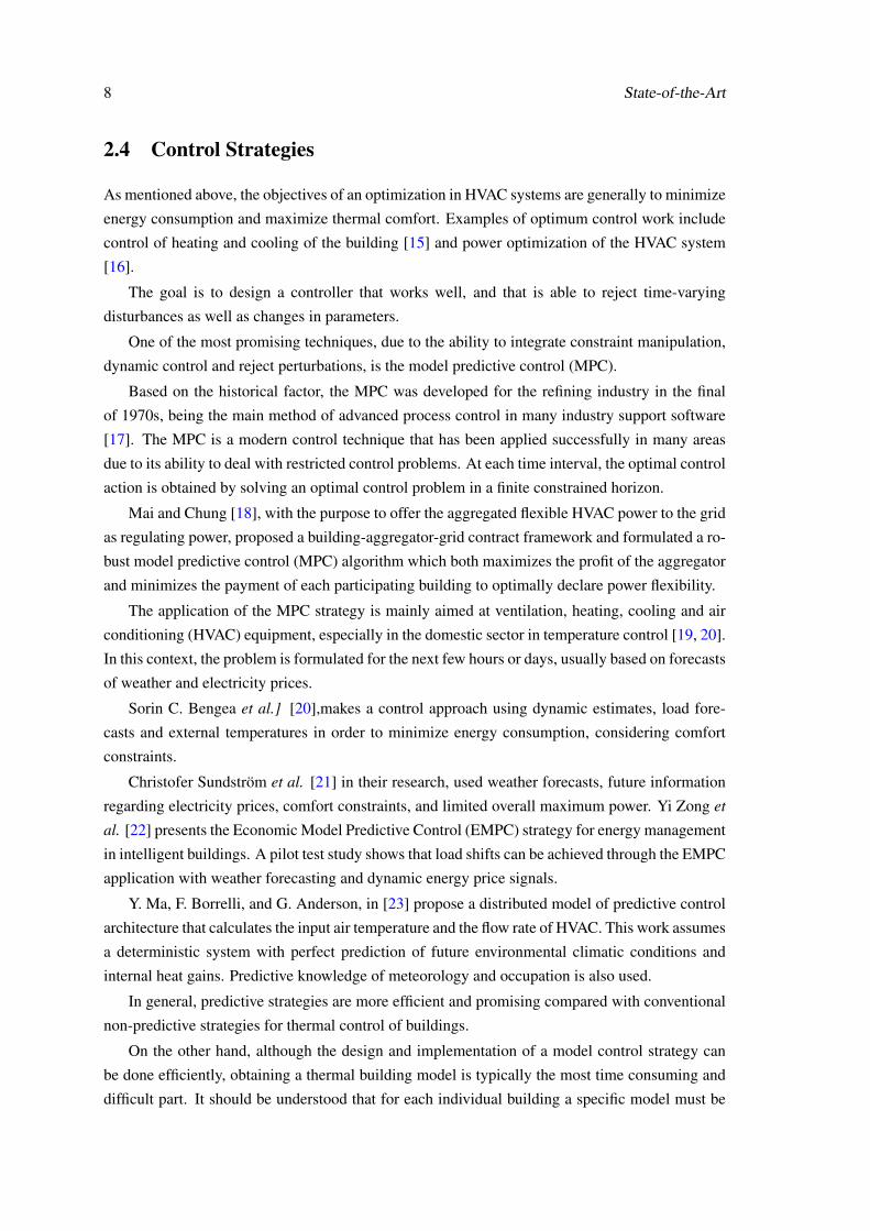
Figure 2.1: Comparison of the white box modeling approach (left) with the grey box modellingapproach(centre) and the black box modeling approach (right) – adapted from [33]

2.7.1 White Box Model

White box models are models with parameters of physical significance and for modelling them a

significant amount of building knowledge is necessary [33].

The parameters of white-box models have physical significance and fundamental physical

principles are used. There are always errors associated with random variables that are not repre-

sented in the known parameters (e.g. window openings and air exchange rates in natural ventila-

tion) [31, 33].

When calibrating white-box models, it makes sense to adapt the less precisely known param-

eters (i.e. heat transmission, heat storage and heat flux), where usually plausible constraints on

these parameters are determined.

2.7.2 Black Box Model

On the other hand, Black-box are empirical models, that is statistical models without physically

significant parameters. Unlike the white-box, we use the black box model when knowledge about

the building system is little [33].

The internal structure of black-box model does not reflect the structure of the building system

phenomena. Black-box models focus on finding the relationships between input and output vari-

ables, independently of the building system phenomena or random variables, which are affecting

the predictive efficiency of the white-box approach.

The parameters are generally adjusted automatically [34]. In comparison with white box mod-

els, this is the best advantage: the automatic adjustment of calibration of black-box parameters.

Furthermore, when there is little information about the system, the black box model is considered

to be inconsistent with physical reality, which is a disadvantage.

Therefore, black-box models are mainly used for error detection, but not for the optimization.

Their advantage is the rapid and automated identification of outputs of thermal energy building

consumption. The structure depends on the relationships between the input and output data.

12 State-of-the-Art

In thermal modelling of buildings, it is reasonable to combine the relative strengths of black-

box coming from the statistical with the white-box strengths based on physical interpretation [33],

[35], in order to obtain an hybrid model. In that sense, the standard grey box approach is based on

both, a statistical method and physical properties that meets the physical fundamental principles.

2.7.3 Grey Box Model

In a simple way, grey-box models are a mix between white-box and black-box models.

If we take into consideration some papers on the matter, there are several and more complex

definitions. The following are the most frequently encountered:

•Grey-box parameters are both empirical and have a physical significance [36]

• Grey-box models are characterized by the fact that all their parameters or a part of them are

determined by measured data of real system [27, 37].

The second definition does not describe any kind of model, but rather the manner of determin-

ing the parameters of a model, something that will be very important in this dissertation.

It is important to be noted that in the literature, often the term Hybrid model emerges to define

grey box model. Regardless of the definitions used, grey box or hybrid models, there is a mixture

of both models without knowing which one dominates in the combination of white-box and black-

box models [27, 37].

Grey box models can be developed for the individual components or for a larger complex

system.

In conclusion, grey-box modelling can increase the optimality of the energy management of

other loads, such as HVAC.

Thus, it is necessary to understand the link between the grey box and the model predictive

control of building systems. That is, to perceive the necessity of the structural model that is behind

the prediction method to improve the performance of buildings and thus achieve the reduction of

energy consumption in heating and cooling systems.

2.8 Load Modelling

When we talk about smart grids context and technologies, one of the most important things is the

prediction methods of energy consumption, and this is the key to the sustainability of the energy

efficiency of the buildings [38].

In order to have a good thermal behaviour model of the building and, in smart grid context, to

increase the efficiency of HVAC systems it is necessary to apply accurate and complete thermal

models for reducing the energy consumption. The model needs to be capable of describing the

different internal and external phenomena of the building.

There are many different approaches to system identification, e.g. [39, 40], that exploit both

the main physical and statistical data of the building system.

It is important to emphasize that in order to define the predictive energy method where the

objective is the improvement of the energy performance of a building as well as the energy saving,

2.8 Load Modelling 13

it is intended to reduce the environmental impact by controlling the energy use over time, moving

the power consumption to off-peak periods [2]. Thus, it becomes critical to describe the response

of the building interior temperature (or in the present thesis, in a room) in the presence of certain

factors such as heat transfer, heat storage, external temperature, radiation, or other internal gains

(computers or people).

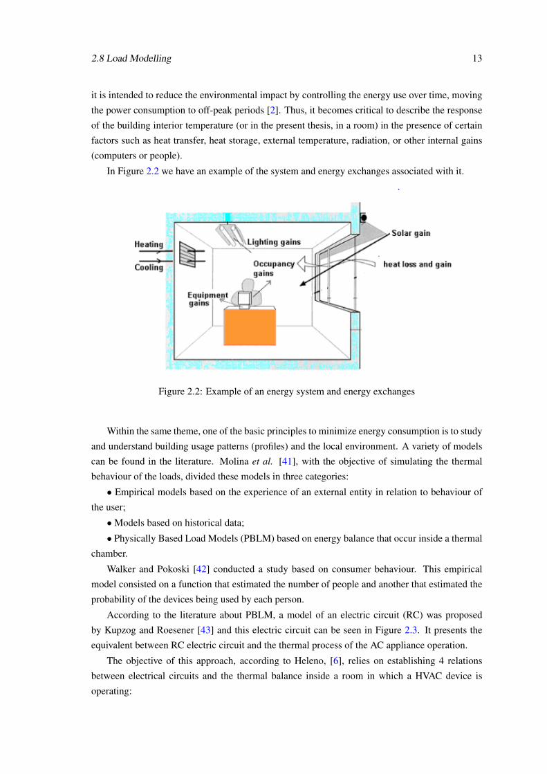
In Figure 2.2 we have an example of the system and energy exchanges associated with it.

Figure 2.2: Example of an energy system and energy exchanges

Within the same theme, one of the basic principles to minimize energy consumption is to study

and understand building usage patterns (profiles) and the local environment. A variety of models

can be found in the literature. Molina et al. [41], with the objective of simulating the thermal

behaviour of the loads, divided these models in three categories:

• Empirical models based on the experience of an external entity in relation to behaviour of

the user;

•Models based on historical data;

• Physically Based Load Models (PBLM) based on energy balance that occur inside a thermal

chamber.

Walker and Pokoski [42] conducted a study based on consumer behaviour. This empirical

model consisted on a function that estimated the number of people and another that estimated the

probability of the devices being used by each person.

According to the literature about PBLM, a model of an electric circuit (RC) was proposed

by Kupzog and Roesener [43] and this electric circuit can be seen in Figure 2.3. It presents the

equivalent between RC electric circuit and the thermal process of the AC appliance operation.

The objective of this approach, according to Heleno, [6], relies on establishing 4 relations

between electrical circuits and the thermal balance inside a room in which a HVAC device is

operating:

14 State-of-the-Art

Figure 2.3: Equivalent between RC electric circuit and AC thermal process – adapted from [43]

1- Electric current and thermal power of the AC heat pump – i.e. the quantity of heat over time

(Q/t);

2- The electric resistance and the total thermal resistance of the room walls;

3- The capacitance of the electric capacitor and the thermal capacity of the room, which de-

pends on the volume of the space as well as on the air composition;

4- The voltage and the temperature.

In addition, it should be noted that there are models of varied complexity. Obviously, simpler

models are easier to simulate. However, they do not realistically represent the behaviour of loads.

On the other hand, the more complex models have better results, although they are more difficult

to implement. With respect to these models, the drawback is that they are computationally heavier,

which implies more information for the simulation, which in fact it is not always easy to obtain.

A very complete description of a house thermal behaviour including AC units has been pro-

posed by Bargiotas and Birdwell [44]. The temperature variation inside the room as well as its

relation with the relative humidity of the air have been considered in this model. On the other hand,

Perfumo et al. [45] proposed a model that describes, in a simpler way, the thermal behaviour. This

model is presented in Equation (2.1).

∂θ(t)∂ t

= − 1CR

[θ(t)−θa +m(t)RP+w(t)] (2.1)

Regarding the equation above presented, θ refers the temperature inside the room and θa is

the outdoor ambient temperature (assumed constant). The thermal capacity (C) and resistance (R)

are elements that are part of the room where the AC appliance is located. The power of the AC

equipment is represented by P. External factors, such as a door or window opening as well as the

presence of computers or any other loads that influence the energy balance are represented by w.

2.9 Parameter Estimation 15

J. Iria et al. [46] in their work proposed a physically based load Equation (2.2) for setting the

temperature inside the room.

θ j ,i,t+1 = βi×θ j ,i,t +(1−βi)(θ j ,0t +COPi×R×Pj ,i,

Tt

CL) (2.2)

Where, βi = e−∆tRC .

Regarding Equation (2.2), D. S. Callaway [47] proposed a very similar model to control ther-

mostatically controlled loads.

The parameters in (2.2) are thermal resistance R(oC/kW), capacitance C(kWh/oC) of the room,

coefficient of performance COPi and outdoor temperature θ j ,0t .

It is understood that the prediction models are necessary to allow the optimal control of the

phenomena of buildings and also to predict the dynamic cooling and heating requirements [48].

One of the main contributors to the quality of the prediction is a well-identified model that will

be used later for the control in the prediction algorithm [40], that is, for HVAC optimization.

Although the model presented in (2.1) can establish a simple relation between the temperature

of the room and the power of the AC unit in a time period, several data are required. Heleno et al.

[7] divides this data in 4 types:

• Physical characteristics of the equipment and environment: capacity and thermal resistance

and nominal electrical power;

• Consumption patterns: the periods when the AC is switched on;

• User comfort requirements: maximum and minimum user-desired temperature in each time

period;

• External and internal variables: room temperature outside and inside the room;

Thus, it is necessary gather the information required. Some of this information is obtained

by collecting data for some time, through the manufacturer, the user himself, measured through

sensors or obtained through calculations. Some information is difficult to measure or is not able to

be obtained through any of the aforementioned methods, which leads to the need to predict certain

information and parameters.

2.9 Parameter Estimation

Parameter estimation boils down to solving an optimization problem, finding the parameter set

that minimizes the error of a scalar function, evaluating over the entire identification data set [33].

For example, for a given estimate of the parameter θ , the prediction error ε(t, θ) can be repre-

sented as the difference between the real value of the output, y(t), and the value determined is y(t

| θ ), that depends on the parameter θ , in a given time.

16 State-of-the-Art

ε(t, θ) = y(t)− y(t|θ) (2.3)

A state estimation can be defined as the process of determining a valid and highly probable

operating point described by the value of a state variable. In other words, state estimation is

responsible for filtering and eliminating inadequate data.

Thus, the state estimation problem can be formulated using the subsequent constrained opti-

mization problem:

minJ(x) (2.4)

Subject to:

c(x) = 0 (2.5)

g(x) ≥ 0 (2.6)

Where c(x) and g(x) correspond to the equality-constraint and inequality-constraint vectors,

accordingly. The objective function is J(x) and represents the total error between the real values

and the estimated values which is intended to be minimized, ε(t, θ).

An experimental methodology was developed, by Holland et al. [49], for online system iden-

tification of a thermal system. Mathematical models were developed for thermal system iden-

tification. The collected temperature data was used to estimate the net thermal resistance and

capacitance using system identification techniques.

Regarding the work performed by El-Ferik et al. [50], an identification problem of the param-

eters of an aggregated elemental physically based model representing a housing unit with an AC

system were developed. The required hardware and system instrumentation are detailed, contain-

ing a sensitivity analysis study of the model for variations in solar radiation and humidity. The

results indicate that the physics-based model was able to capture the effects of outdoor conditions.

About online building thermal parameter estimation, Peter Radecki et al. [51] demonstrate

how an Unscented Kalman Filter augmented for parameter estimation can accurately learn and

predict a building’s thermal response. A grey-box approach using an Unscented Kalman Fil-

ter based on a multi-zone thermal network was proposed and it was validated with EnergyPlus

simulation data. The filter learns parameters of a thermal network during periods of known or

constrained loads and then characterizes unknown loads in order to provide accurate 48+ hour

energy predictions. In addition, Peter Radecki et al. said that recent studies of buildings’ heating,

2.9 Parameter Estimation 17

ventilating, and air conditioning systems have shown 25% to 30% energy conservation is possible

with advanced control systems.

18 State-of-the-Art

Chapter 3

Methodology

This dissertation aims to create a thermal model of a room, determining certain parameters of

the room, which influence the thermal behaviour, and perceive the impact they may have on the

temperature.

The objective of creating a thermal model and determining these parameters is to predict room

temperature over a 24-hour time horizon, with a 15-min granularity, and through the parameters

and variables estimated to be able to make an optimization model for certain loads. In this disser-

tation, it will be considered an Air Conditioner (AC), since in addition to being controlled, in a

house or in a corporate building this load is responsible for the majority of the energy consumption.

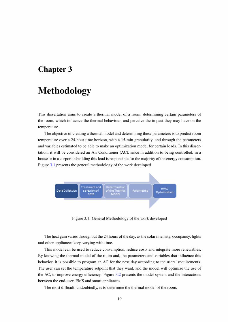
Figure 3.1 presents the general methodology of the work developed.

Figure 3.1: General Methodology of the work developed

The heat gain varies throughout the 24 hours of the day, as the solar intensity, occupancy, lights

and other appliances keep varying with time.

This model can be used to reduce consumption, reduce costs and integrate more renewables.

By knowing the thermal model of the room and, the parameters and variables that influence this

behavior, it is possible to program an AC for the next day according to the users’ requirements.

The user can set the temperature setpoint that they want, and the model will optimize the use of

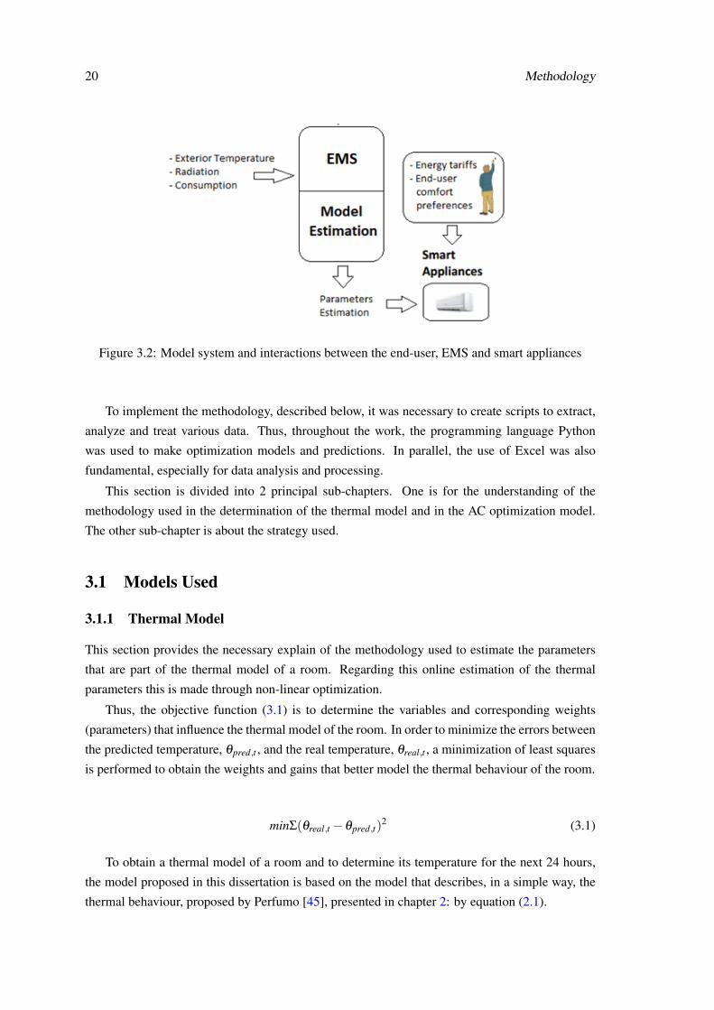
the AC, to improve energy efficiency. Figure 3.2 presents the model system and the interactions

between the end-user, EMS and smart appliances.

The most difficult, undoubtedly, is to determine the thermal model of the room.

19

20 Methodology

Figure 3.2: Model system and interactions between the end-user, EMS and smart appliances

To implement the methodology, described below, it was necessary to create scripts to extract,

analyze and treat various data. Thus, throughout the work, the programming language Python

was used to make optimization models and predictions. In parallel, the use of Excel was also

fundamental, especially for data analysis and processing.

This section is divided into 2 principal sub-chapters. One is for the understanding of the

methodology used in the determination of the thermal model and in the AC optimization model.

The other sub-chapter is about the strategy used.

3.1 Models Used

3.1.1 Thermal Model

This section provides the necessary explain of the methodology used to estimate the parameters

that are part of the thermal model of a room. Regarding this online estimation of the thermal

parameters this is made through non-linear optimization.

Thus, the objective function (3.1) is to determine the variables and corresponding weights

(parameters) that influence the thermal model of the room. In order to minimize the errors between

the predicted temperature, θpred,t , and the real temperature, θreal,t , a minimization of least squares

is performed to obtain the weights and gains that better model the thermal behaviour of the room.

minΣ(θreal,t −θpred,t)2 (3.1)

To obtain a thermal model of a room and to determine its temperature for the next 24 hours,

the model proposed in this dissertation is based on the model that describes, in a simple way, the

thermal behaviour, proposed by Perfumo [45], presented in chapter 2: by equation (2.1).

3.1 Models Used 21

The model presented below in Equation (3.2) and in Equation (3.3) are shaped according to

the information we have access and the implementation strategy (something that will be discussed

in more detail in Chapter 4. There are two equations, because in our model we consider different

parameters for weekdays (3.2) and days of weekend or holiday (3.3).

θt+1 = θt −∆tRC

(θt −θ0t )−

∆tC(m×Pt −Const ×wC,t −Radt ×wR,t −wE,t),∀t ∈ N (3.2)

θt+1 = θt −∆tRC

(θt −θ0t )−

∆tC(m×Pt −Const ×w_ f sC,t

−Radt ×w_ f sR,t −w_ f sE,t), ∀t ∈ N(3.3)

Where θt refers to the temperature inside the room at the time “t” and θ 0t is the outdoor ambient

temperature. So, (θt−θ 0t ) represents the change of indoor temperature with the energy exchanges

with the exterior. External factors like a door or window opened as well other energy exchanges

that could not be predicted are represented by wE,t for weekdays, and by w_ f sE,t for weekends or

holidays.

These energy exchanges may be gains or losses. The thermal capacity (C) and resistance (R)

are elements that are part of the room and are influenced by its area. The electric power of the AC

equipment is represented by P and the efficiency level is represented by m. This last index differs

in case of heating or cooling (COP and EER) and depends on the AC. COP is the coefficient of

performance and it is used for heating, whereas EER is the energy efficiency ratio and it is used

for cooling.

It should be noted that in a room there are other gains that derive from, for example, lighting,

people and appliances such as computers. Thus, in this model it is considered that, Const repre-

sents the electric power consumption of the room at the time “t” and it is multiplied by a weight,

wC,t for weekdays and w_ f sC,t for weekends or holidays. The complete formulation of the model

includes this limits that are influenced by the maximum of people, computers and lights inside the

room and this can be represented by the Equation (3.4) for weekdays and (3.5) for weekends or

holidays.

0≤Const ×wC,t ≤ PmaxPC(kW )+Pmaxpeople(kW )+Pmaxlamps(kW ),∀t ∈ N (3.4)

0≤Const ×w_ f sC,t ≤ PmaxPC(kW )+Pmaxpeople(kW )+Pmaxlamps(kW ),∀t ∈ N (3.5)

It is important to mention that the consumption will model the gain that comes from computers,

people or lights. This means that, when there is energy consumption it is understood that there are

22 Methodology

thermal gains. The people’s behaviour in the room can be translated through the behaviour of the

energy consumption.

On the other hand, a factor that greatly influences the internal temperature of a room, espe-

cially if it has windows, is the external incident radiation. Thus, Radt ×wR,t represents the gain

derived from radiation for a weekday, Equation (3.6) and Radt ×w_ f sR,t for weekends or holi-

days, Equation (3.7). Radt represents the incident radiation at time “t” and wR,t (or w_ f sR,t) is the

related weight that needed to determine.

Radt ×wC,t ≥ 0,∀t ∈ N (3.6)

Radt ×w_ f sC,t ≥ 0,∀t ∈ N (3.7)

It is important to highlight that in this thesis model it is necessary to have access to the infor-

mation about the consumption and the radiation, as well as the external ambient temperature.

The problem model, was performed by using PYOMO that is a Python-based open-source

software package that supports a diverse set of optimization capabilities for formulating, solving,

and analyzing optimization models [52].

The solver used in the optimization model used it was IPOPT (Interior Point Optimizer). This

is an open source software package for large-scale nonlinear optimization [53]. It is designed to

find (local) solutions of mathematical optimization problems of minimization form. It is possible

to use PYOMO and the solver IPOPT integrated in Python scripting language.

In relation to the Equation (3.2) or (3.3), to be better understood, the variables and their units

are presented in Table 3.1.

Table 3.1: Variables and respective units

Variable Unitθ oC∆t hC kWh

oCR

oCkW

P kWCons kWRad kW

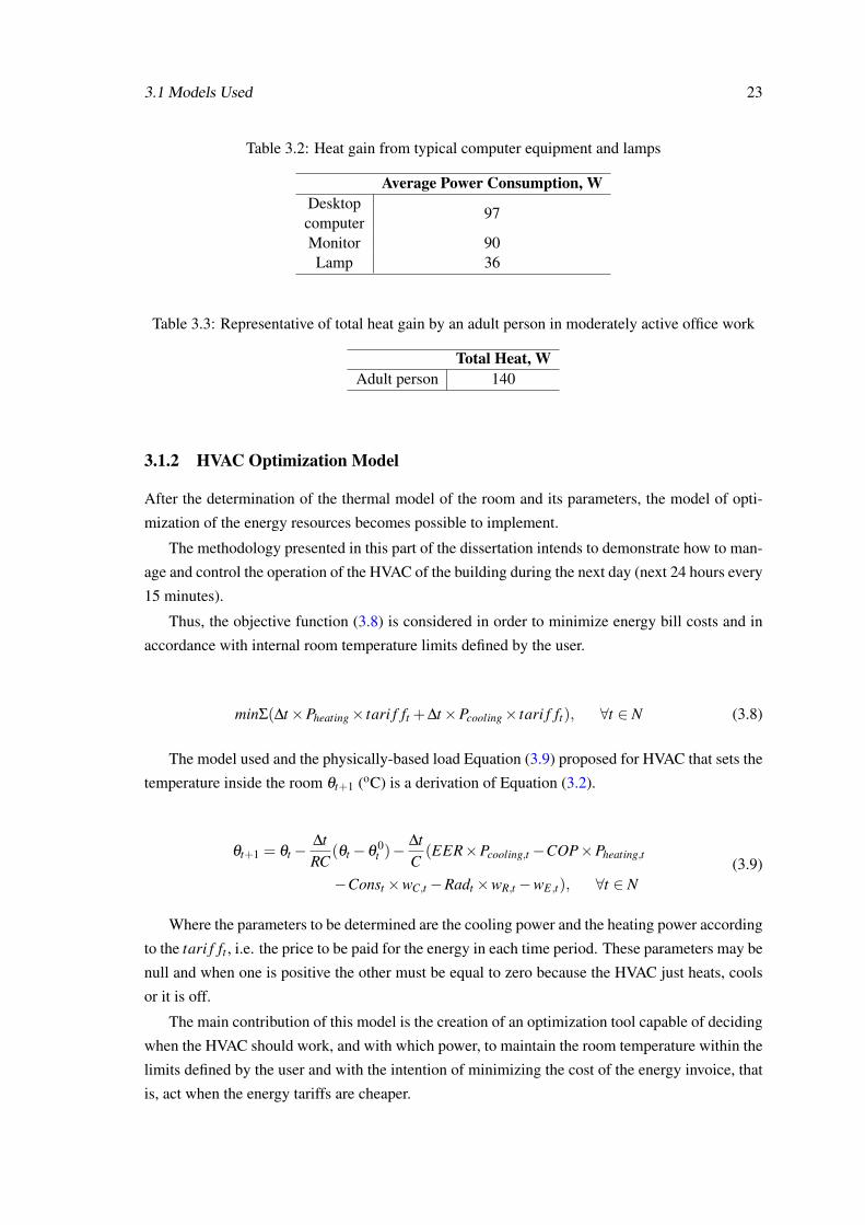
Regarding the heat gains by computers and lighting, Table 3.2 presents the considered values.

Heat gains from people are presented in Table 3.3. It should be noted that these are values com-

monly used in the literature. The heat transmitted through a lamp is related to its power, and it is

a characteristic that depends on each lamp. In this case, the lamp has a power of 36 W.

The information about the typical heat from computers and people was extracted from [54].

3.1 Models Used 23

Table 3.2: Heat gain from typical computer equipment and lamps

Average Power Consumption, WDesktopcomputer

97

Monitor 90Lamp 36

Table 3.3: Representative of total heat gain by an adult person in moderately active office work

Total Heat, WAdult person 140

3.1.2 HVAC Optimization Model

After the determination of the thermal model of the room and its parameters, the model of opti-

mization of the energy resources becomes possible to implement.

The methodology presented in this part of the dissertation intends to demonstrate how to man-

age and control the operation of the HVAC of the building during the next day (next 24 hours every

15 minutes).

Thus, the objective function (3.8) is considered in order to minimize energy bill costs and in

accordance with internal room temperature limits defined by the user.

minΣ(∆t×Pheating× tari f ft +∆t×Pcooling× tari f ft), ∀t ∈ N (3.8)

The model used and the physically-based load Equation (3.9) proposed for HVAC that sets the

temperature inside the room θt+1 (oC) is a derivation of Equation (3.2).

θt+1 = θt −∆tRC

(θt −θ0t )−

∆tC(EER×Pcooling,t −COP×Pheating,t

−Const ×wC,t −Radt ×wR,t −wE,t), ∀t ∈ N(3.9)

Where the parameters to be determined are the cooling power and the heating power according

to the tari f ft , i.e. the price to be paid for the energy in each time period. These parameters may be

null and when one is positive the other must be equal to zero because the HVAC just heats, cools

or it is off.

The main contribution of this model is the creation of an optimization tool capable of deciding

when the HVAC should work, and with which power, to maintain the room temperature within the

limits defined by the user and with the intention of minimizing the cost of the energy invoice, that

is, act when the energy tariffs are cheaper.

24 Methodology

It should be noted that in this model only the power provided by the HVAC is determined

for each time interval, because the thermal model is already defined, and the room temperature is

already known without the optimization of the HVAC.

However, it is important to note that a HVAC is limited by a maximum power, both for heating

or cooling, being something specified in the datasheet of the model.

Thus, for the optimization model it is necessary to consider the maximum power limits and

the comfort temperature limits established by the user. These restrictions are defined by Equations

(3.10) and (3.11).

0≤ Pcooling,t ≤ Pmax, 0≤ Pheating,t ≤ Pmax (3.10)

θmin ≤ θt+1 ≤ θmax (3.11)

The problem is modeled, again, through the PYOMO and the solver used was the GLPK

(GNU Linear Programming Kit). This is a software package developed to solve large-scale linear

programming (LP), mixed integer programming (MIP), and other related problems [55]. It is also

possible to use GLPK integrated with Python scripting language.

Regarding tariffs, the information is easy to obtain because it is something that is tabulated and

specified in the energy bill. This depends on the contract and on the customer, since, for instance,

a low voltage customer has different tariffs from a medium voltage customer.

3.2 Strategy Used

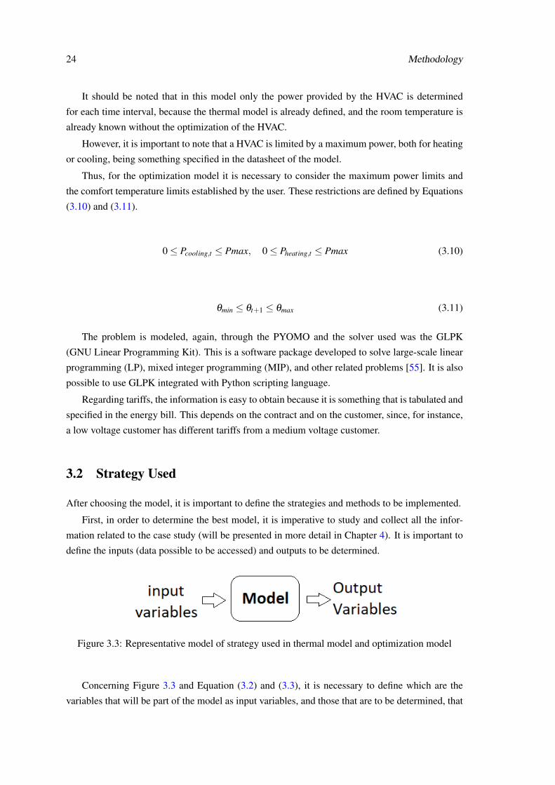
After choosing the model, it is important to define the strategies and methods to be implemented.

First, in order to determine the best model, it is imperative to study and collect all the infor-

mation related to the case study (will be presented in more detail in Chapter 4). It is important to

define the inputs (data possible to be accessed) and outputs to be determined.

Figure 3.3: Representative model of strategy used in thermal model and optimization model

Concerning Figure 3.3 and Equation (3.2) and (3.3), it is necessary to define which are the

variables that will be part of the model as input variables, and those that are to be determined, that

3.2 Strategy Used 25

is, output variables. The objective is predicting the room temperature for a certain day (every 15

minutes over 24 hours).

Thus, Table 3.4 presents the input variables and the parameters that we want to determine.

Table 3.4: Symbol of input variables and outputs that we intend to determine

Input Variables Output Variablesθt Cθ 0

t Rm wE,t

P wC,t

Cons wR,t

Rad

Regarding the variables to be determined, different variables and weights were defined for

weekend days, holidays and weekdays, since this was identified as the approach that would lead to

best results. It was stipulated that a holiday behaviour would be equivalent to the behaviour shown

on a weekend day. For example, during the week we see a higher energy consumption than at the

weekend or on a holiday.

As the main objective was the determination of parameters and thermal gains of the room for

the modelling of thermal behaviour, the data used for training was the data corresponding to a

month’s period, that is, by minimizing the square errors, we determined a set of parameters with

the least possible error for a month. Following this, the Equation 3.1 of the thermal model was

applied in order to determine the parameters and variables to predict the room temperature.

In order to test the model, the latter was compared to the test data. The real temperature data

was extracted through a temperature sensor. This comparison consisted in verifying the waveform

and its behaviour, as well as the mean absolute error (MAE). Equation (3.12) presents the MAE

formula that measures the average magnitude of the errors in a set of predictions. It’s the average

over the test sample of the absolute differences between prediction and actual observation where

all individual differences have equal weight.

MAE =1n

n

∑t=1|θreal,t −θpred,t | (3.12)

In summary, an extended set of training days, one month, was used and later the model was

tested for different days from the training set, that is, test days. The waveform and the MAE

were analysed to validate the model. To select the best model, the MAE was verified not only for

specific days but for a whole week.

So, it is crucial to define the best strategy to obtain all the available information, that is, to

obtain all the inputs for the model.

The strategies implemented to obtain all the necessary information for the model are presented

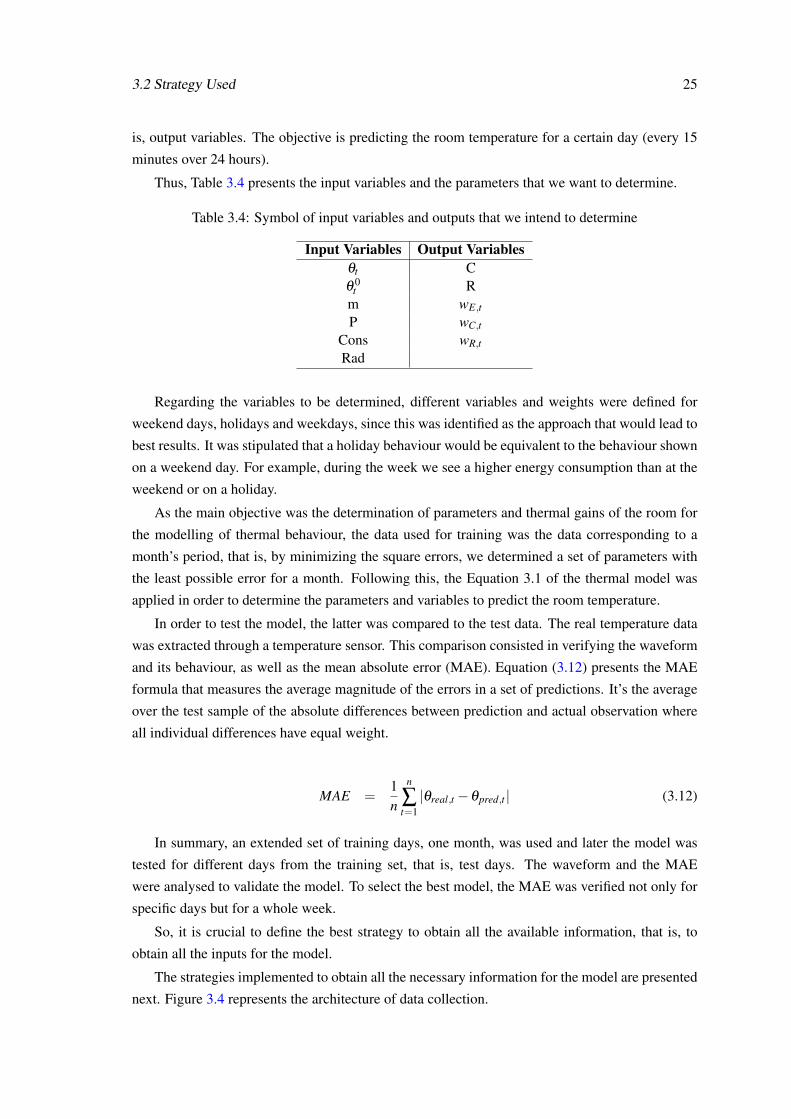
next. Figure 3.4 represents the architecture of data collection.

26 Methodology

Figure 3.4: System architecture of data collection

• Internal Temperatures: Sensors were used to collect data of the internal temperatures of

the room. These recorded room temperatures every 15 minutes.

• Energy Consumption: Smart meters were used with the purpose of measuring the en-

ergy consumption of the room and these were installed in the electrical board. The meters

used were developed by WITHUS, a Portuguese company. The energy consumption was

recorded every 15 minutes.

It is important to emphasize that in relation to the test model, a perfect forecast for con-

sumption was applied.

• External Temperatures: Forecasts were used for the collection of external temperatures. A

program in Python language was implemented to extract the information from [56], which

provides temperature forecasts for given geographic location.

• Radiation: To collect the radiation data we resorted to forecasts A program in Python

language was implemented to extract the information from [56], which provides temperature

forecasts for desired given geographic location.

It should be noted that the external temperature and radiation forecasts were collected every

hour. Thus, to maintain coherence with the other data, it was assumed that the external

temperature and radiation only changed in an hourly basics, that is, for a given hour there

are four equal and unchanged values, because in one hour there are four periods of 15

minutes.

• AC Power: AC power values were collected through the meters and the results were saved

every 15 minutes.

3.2 Strategy Used 27

Regarding the AC, it was necessary to analyse the datasheet to know the coefficients COP and

EER, as well as the maximum power to heat and to cool.

Furthermore, to implement the model, it was necessary to limit certain gains, such as gains

derived from consumption. For this, it is necessary to study the room and determine the maximum

number of people who usually are in the room, as well as the number of computers and the number

of lamps. After determining the amount of these elements, it is possible to know the limit of the

thermal gain affected by these, and thus, limit the consumption for each 15 minutes, for the best

thermal modelling.

It was decided that both radiation and consumption would be represented as gains, that is, they

would influence the heating of the room. On the other hand, there are other gains (or losses) of

energy exchanges with other rooms or the exterior, due to the opening of windows or doors, for

example. Thus, in Equation (3.1) the variable wE,t represents the energy exchanges, which can be

thermal gains or losses. Regarding the model and the parameters to be determined, these have a

different behaviour for weekdays and weekend days or holidays, as above mentioned. During the

training, one model was defined for the week and another for the weekend.

With the purpose of understanding the influence and impact of certain variables in the model,

such as consumption and radiation, it was necessary to test several models first to see how the in-

troduction of these parameters would affect the thermal modelling of the room. Thus, the strategy

started with a simple model with few variables and by checking the results obtained and by adding

new parameters and restrictions, the best model was achieved.

In addition, it was fundamental to analyse the behaviour of the use of energy equipment, that

is, the behaviour of the consumption of the room. With this analysis it is possible to know when

there are people in the room and the periods when energy consumption is higher.

Finally, with regard to the modelling of the AC and after the thermal model was defined and

all parameters determined, the energy invoice of the INESC TEC building (demo site used in this

thesis) was checked to know the present tariffs and thus to be able to model the AC considering

energy prices.

After implementing the strategy, to consolidate and perceive even better the work described, it

is important to analyse the case study and the results obtained in order to prove the effectiveness

of the proposed models.

28 Methodology

Chapter 4

Case Study and Analysis of Results

4.1 Case Study

In this part of the chapter, the case study and all the characteristics associated with it are presented.

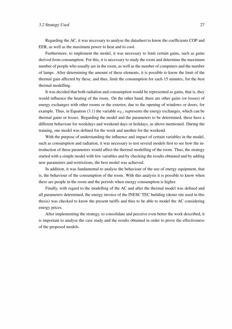
Figure 4.1 presents the floor plan of the room from which the model was developed and tested.

Figure 4.1: Floor plan of the case study room

All data and information collected were designed to determine the thermal model of this room.

As it can be seen in Figure 4.1, there is a temperature sensor placed strategically with the

purpose of measuring the room’s internal temperature every 15 minutes. This data served first as

the input database and afterwards as basis of comparison with the test models. It should be noted

that the sensor was placed in a safe and high position where human influence was reduced, so

that the data was as correct as possible, since the sensor does not present a completely accurate

temperature, since it has a measurement error. In the present case, the sensor used was the EL-

USB-1-LCD of the brand EasyLog. According to [57], the sensor has an overall error of ±0,5oC.

In addition to the sensor, a smart meter was installed in the electrical panel that recorded the

consumption of the room’s outlets (where computers are connected, for example) and the AC

consumption.

Although in the same figure it is possible to understand that there are 3 rooms with different

areas, in the case of study the 3 areas are considered as one, mainly due to the fact that the doors

that connect these rooms are open most of the time. The total area of the room is 84m2. In addition,

29

30 Case Study and Analysis of Results

the consumption that is accessed through the smart meters corresponds to the set of three rooms.

Due to that, throughout the dissertation, references to the “room” should be understood as the total

area of the 3 spaces.

The choice of this room to test the model was because it has a split air conditioner itself. It

should be noted that the INESC TEC building has a centralized AC, and there are only a few rooms

with its own AC. Regarding the AC characteristics, it was necessary to analyse its datasheet to

collect the necessary information. Table 4.1 presents the AC model and some of its characteristics.

Table 4.1: Necessary information extracted from datasheet of the AC model

Model FCQG60FVEBCooling Power Min./Nom./Max. (kW) 1.7/5.7/5.7Heating Power Min./Nom./Max. (kW) 1.7/7.0/7.0

Cooling Supply Power Min./Nom./Max. (kW) -/1.640/-Heating Supply Power Min./Nom./Max. (kW) -/1.990/-

Nominal Efficiency - EER 3.48Nominal Efficincy - COP 3.52

It should be noted that a study was made to see if the AC had been used to heat up or cool

down the room during the training data. First, it was concluded that the AC was used only a few

times. In addition, it was concluded that the AC was only used to cool down the room. Thus, the

model was implemented with the EER cooling factor. This is something of great importance to

the training and modelling part.

With respect to thermal modelling, the room area is of great importance because both the

thermal resistance and the capacitance are influenced by it. According to DS Callaway [47], the

capacitance C varies from 0.015 to 0.065 kWh / oC per square meter of floor space, and the thermal

conductance (= 1 / R) ranges from approximately 0.001 (for a very efficient building) to 0.003 kW

/ per square meter. It is important to note that the parameters are scaled by floor space because,

although the volume and surface area are more natural variables to scale thermal mass and thermal

resistance, respectively, floor space is a more readily available measure.

Given this, and according to the room area, 84 m2, Table 4.2 shows the ranges of values for R

and C.

Table 4.2: Range values for Resistance and Thermal Capacity

R (oC/kW) C (kWh/oC)3.968 - 11.905 1.260 - 5.460

The measurement of the consumptions is something of great importance because it models the

behaviour of the people and, as such, influences the thermal behaviour of a room. A room where

there are people has a very different thermal behaviour from an empty room for example.

Thus, the measurement of consumption is essential and can be observed in both Figure 4.2

and Figure 4.3. These charts present the consumption of the room for several days of a week and

allow obtaining relevant information regarding people’s behaviour. It is easy to understand that

4.1 Case Study 31

people’s behaviour influences in a significant manner the consumption of the room. If there is no

consumption it can be concluded that there are no people in the room.

Figure 4.2: Consumption every 15 minutes for each day of one week (from 6/11/2017 to12/11/2017)

Figure 4.3: Consumption every 15 minutes for each day of a week (from 30/10/2017 to 5/11/2017)

After analysis and observation of Figure 4.2 or 4.3, it is easy to see that consumption differs

from day to day, having an approximate behaviour for days of the week and a different behaviour

for the weekend days. Saturday and Sunday have a similar behaviour. Of course, this is expected

since people work during the week and as such, consumption is higher on these days. It is also

noted that in weekdays consumption increases approximately from 9 a.m. (36/4 = 9) and decreases

afterwards when most people leave work, around 7:00 p.m. (76/4 = 19).

In addition, it is noted that there is a decrease in consumption at lunchtime, as expected,

increasing again when people return to the room.

The Figure 4.3 is interesting because it can be observed a day of the week, Wednesday, where

the consumptions were quite similar to ones of the weekend. This can be explained by the fact that

it was a holiday, so it can be concluded that the behaviour of this kind of days is very similarly to

the one of the weekend.

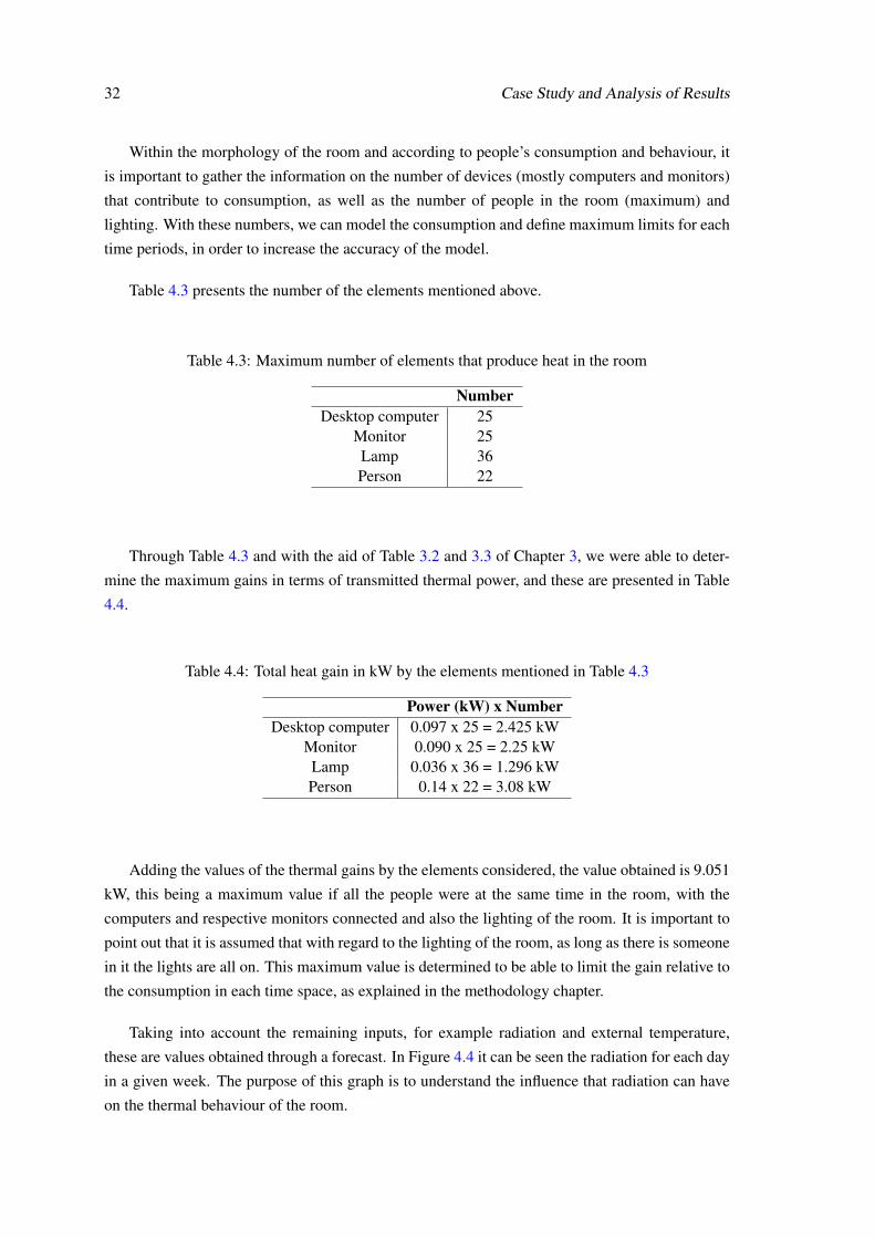
32 Case Study and Analysis of Results

Within the morphology of the room and according to people’s consumption and behaviour, it

is important to gather the information on the number of devices (mostly computers and monitors)

that contribute to consumption, as well as the number of people in the room (maximum) and

lighting. With these numbers, we can model the consumption and define maximum limits for each

time periods, in order to increase the accuracy of the model.

Table 4.3 presents the number of the elements mentioned above.

Table 4.3: Maximum number of elements that produce heat in the room

NumberDesktop computer 25

Monitor 25Lamp 36Person 22

Through Table 4.3 and with the aid of Table 3.2 and 3.3 of Chapter 3, we were able to deter-

mine the maximum gains in terms of transmitted thermal power, and these are presented in Table

4.4.

Table 4.4: Total heat gain in kW by the elements mentioned in Table 4.3

Power (kW) x NumberDesktop computer 0.097 x 25 = 2.425 kW

Monitor 0.090 x 25 = 2.25 kWLamp 0.036 x 36 = 1.296 kWPerson 0.14 x 22 = 3.08 kW

Adding the values of the thermal gains by the elements considered, the value obtained is 9.051

kW, this being a maximum value if all the people were at the same time in the room, with the

computers and respective monitors connected and also the lighting of the room. It is important to

point out that it is assumed that with regard to the lighting of the room, as long as there is someone

in it the lights are all on. This maximum value is determined to be able to limit the gain relative to

the consumption in each time space, as explained in the methodology chapter.

Taking into account the remaining inputs, for example radiation and external temperature,

these are values obtained through a forecast. In Figure 4.4 it can be seen the radiation for each day

in a given week. The purpose of this graph is to understand the influence that radiation can have

on the thermal behaviour of the room.

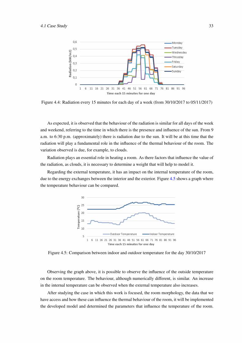
4.1 Case Study 33

Figure 4.4: Radiation every 15 minutes for each day of a week (from 30/10/2017 to 05/11/2017)

As expected, it is observed that the behaviour of the radiation is similar for all days of the week

and weekend, referring to the time in which there is the presence and influence of the sun. From 9

a.m. to 6:30 p.m. (approximately) there is radiation due to the sun. It will be at this time that the

radiation will play a fundamental role in the influence of the thermal behaviour of the room. The

variation observed is due, for example, to clouds.

Radiation plays an essential role in heating a room. As there factors that influence the value of

the radiation, as clouds, it is necessary to determine a weight that will help to model it.

Regarding the external temperature, it has an impact on the internal temperature of the room,

due to the energy exchanges between the interior and the exterior. Figure 4.5 shows a graph where

the temperature behaviour can be compared.

Figure 4.5: Comparison between indoor and outdoor temperature for the day 30/10/2017

Observing the graph above, it is possible to observe the influence of the outside temperature

on the room temperature. The behaviour, although numerically different, is similar. An increase

in the internal temperature can be observed when the external temperature also increases.

After studying the case in which this work is focused, the room morphology, the data that we

have access and how these can influence the thermal behaviour of the room, it will be implemented

the developed model and determined the parameters that influence the temperature of the room.

34 Case Study and Analysis of Results

The next subchapter will describe the work done in detail, starting by analysing a simple mode

and ending with the final and complete model.

4.2 Analysis of Results

4.2.1 Thermal Model

In general, the determination of a thermal model and the parameters that most influence the thermal

behaviour is not a simple task, because, in addition to measuring and predicting errors, it involves

an intensive study and treatment of several data. Furthermore, assumptions and simplifications

need to be made, without compromising the model validity.

It is important to point out that, besides studying the available data, characterising the room and

defining the strategy to be implemented, to obtain a certain model that is feasible, it is necessary

to make several tests, many attempts and verifications.

In this part of the dissertation, some of the results obtained and how they were achieved will

be presented.

Following the strategy explained in Chapter 3, for training, data from 19/10/2017 to 23/11/2017

was used. After the training, at first, the parameters were determined and used to predict the ther-

mal behaviour for a given day. The day used was 24/11/2017.

Firstly, in order to reach the final model, we started with a simpler one, with less variables and

parameters, which is represented by case 1.

It is important not to forget that in this part of the work the comparison was made just for one

day, with the objective of obtaining the best model in terms of waveform, MAE and meaning of

the determined parameters.

Case 1:

In this case, we opted for something very simple, where only the influence of outdoor tem-

perature and AC (which, as mentioned above, on most days was not used) was chosen. Thus, the

model for this case is presented in Equation (4.1) and the parameters to be determined are only C

and R.

θt+1 = θt −∆tRC

(θt −θ0t )−

∆tC(EER×Pt) (4.1)

The results obtained for the forecast temperature through this model can be observed in Figure

4.6. The obtained results do not demonstrate a good approximation to the reality, not demonstrat-

ing a good thermal behaviour of the room.

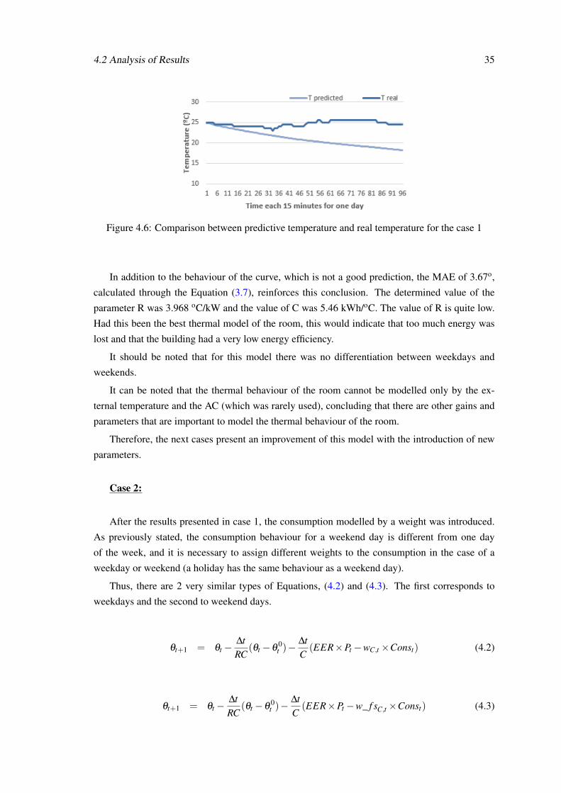
4.2 Analysis of Results 35

Figure 4.6: Comparison between predictive temperature and real temperature for the case 1

In addition to the behaviour of the curve, which is not a good prediction, the MAE of 3.67o,

calculated through the Equation (3.7), reinforces this conclusion. The determined value of the

parameter R was 3.968 oC/kW and the value of C was 5.46 kWh/oC. The value of R is quite low.

Had this been the best thermal model of the room, this would indicate that too much energy was

lost and that the building had a very low energy efficiency.

It should be noted that for this model there was no differentiation between weekdays and

weekends.

It can be noted that the thermal behaviour of the room cannot be modelled only by the ex-

ternal temperature and the AC (which was rarely used), concluding that there are other gains and

parameters that are important to model the thermal behaviour of the room.

Therefore, the next cases present an improvement of this model with the introduction of new

parameters.

Case 2:

After the results presented in case 1, the consumption modelled by a weight was introduced.

As previously stated, the consumption behaviour for a weekend day is different from one day

of the week, and it is necessary to assign different weights to the consumption in the case of a

weekday or weekend (a holiday has the same behaviour as a weekend day).

Thus, there are 2 very similar types of Equations, (4.2) and (4.3). The first corresponds to

weekdays and the second to weekend days.

θt+1 = θt −∆tRC

(θt −θ0t )−

∆tC(EER×Pt −wC,t ×Const) (4.2)

θt+1 = θt −∆tRC

(θt −θ0t )−

∆tC(EER×Pt −w_ f sC,t ×Const) (4.3)

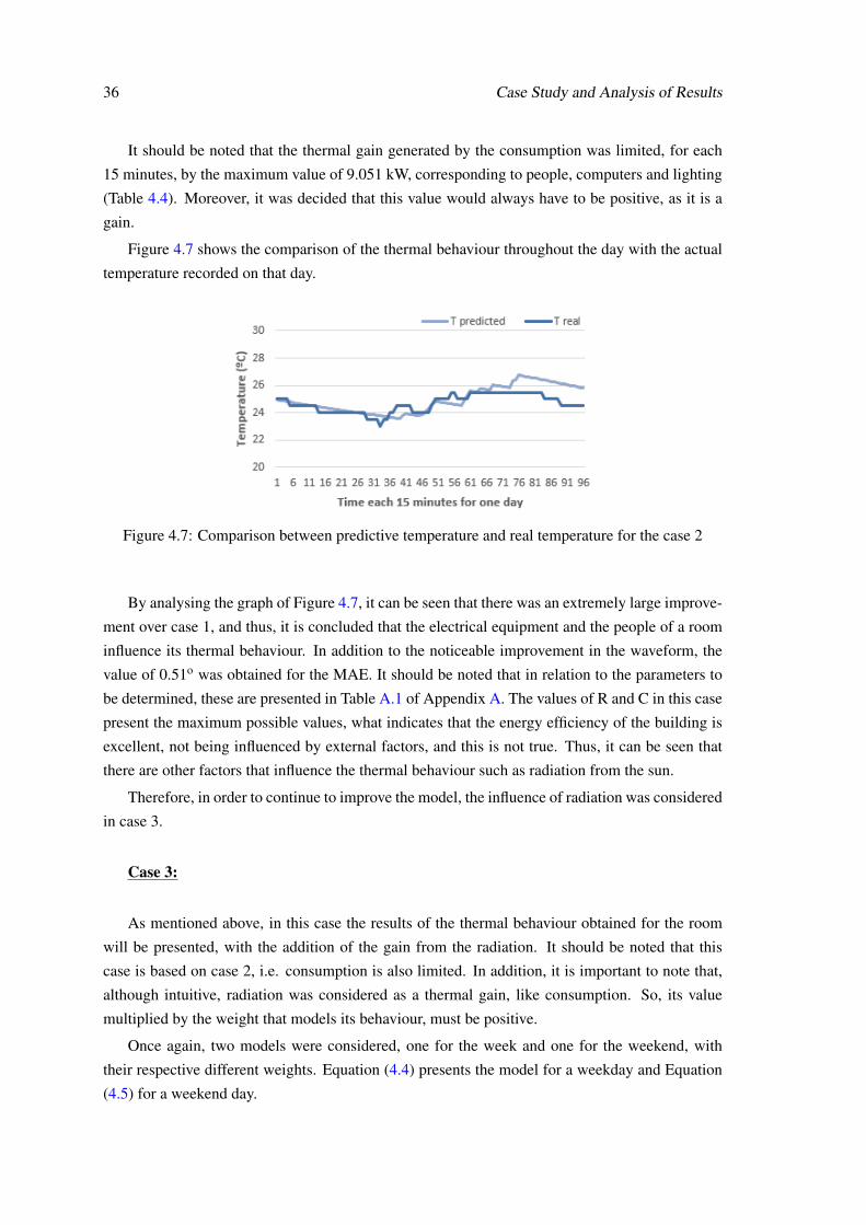
36 Case Study and Analysis of Results

It should be noted that the thermal gain generated by the consumption was limited, for each

15 minutes, by the maximum value of 9.051 kW, corresponding to people, computers and lighting

(Table 4.4). Moreover, it was decided that this value would always have to be positive, as it is a

gain.

Figure 4.7 shows the comparison of the thermal behaviour throughout the day with the actual

temperature recorded on that day.

Figure 4.7: Comparison between predictive temperature and real temperature for the case 2

By analysing the graph of Figure 4.7, it can be seen that there was an extremely large improve-

ment over case 1, and thus, it is concluded that the electrical equipment and the people of a room

influence its thermal behaviour. In addition to the noticeable improvement in the waveform, the

value of 0.51o was obtained for the MAE. It should be noted that in relation to the parameters to

be determined, these are presented in Table A.1 of Appendix A. The values of R and C in this case

present the maximum possible values, what indicates that the energy efficiency of the building is

excellent, not being influenced by external factors, and this is not true. Thus, it can be seen that

there are other factors that influence the thermal behaviour such as radiation from the sun.

Therefore, in order to continue to improve the model, the influence of radiation was considered

in case 3.

Case 3:

As mentioned above, in this case the results of the thermal behaviour obtained for the room

will be presented, with the addition of the gain from the radiation. It should be noted that this

case is based on case 2, i.e. consumption is also limited. In addition, it is important to note that,

although intuitive, radiation was considered as a thermal gain, like consumption. So, its value

multiplied by the weight that models its behaviour, must be positive.

Once again, two models were considered, one for the week and one for the weekend, with

their respective different weights. Equation (4.4) presents the model for a weekday and Equation

(4.5) for a weekend day.

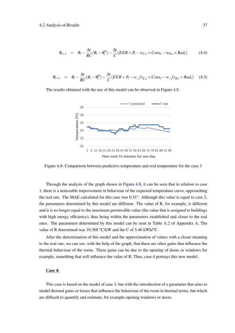
4.2 Analysis of Results 37

θt+1 = θt −∆tRC

(θt −θ0t )−

∆tC(EER×Pt −wC,t ×Const −wR,t ×Radt) (4.4)

θt+1 = θt −∆tRC

(θt −θ0t )−

∆tC(EER×Pt −w_ f sC,t ×Const −w_ f sR,t ×Radt) (4.5)

The results obtained with the use of this model can be observed in Figure 4.8.

Figure 4.8: Comparison between predictive temperature and real temperature for the case 3

Through the analysis of the graph shown in Figure 4.8, it can be seen that in relation to case

1, there is a noticeable improvement in behaviour of the expected temperature curve, approaching

the real one. The MAE calculated for this case was 0.51o. Although this value is equal to case 2,

the parameters determined by this model are different. The value of R, for example, is different

and it is no longer equal to the maximum permissible value (the value that is assigned to buildings

with high energy efficiency), thus being within the parameters established and closer to the real

ones. The parameters determined by this model can be seen in Table A.2 of Appendix A. The

value of R determined was 10.368 oC/kW and the C of 5.46 kWh/oC.

After the determination of this model and the approximation of values with a closer meaning

to the real one, we can see, with the help of the graph, that there are other gains that influence the

thermal behaviour of the room. These gains can be due to the opening of doors or windows for

example, something that will influence the value of R. Thus, case 4 portrays this new model.

Case 4:

This case is based on the model of case 3, but with the introduction of a parameter that aims to

model thermal gains or losses that influence the behaviour of the room in thermal terms, but which

are difficult to quantify and estimate, for example opening windows or doors.

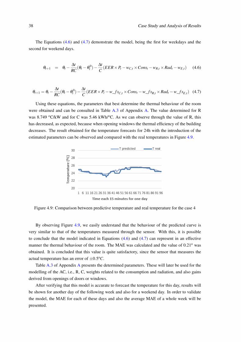
38 Case Study and Analysis of Results

The Equations (4.6) and (4.7) demonstrate the model, being the first for weekdays and the

second for weekend days.

θt+1 = θt −∆tRC

(θt −θ0t )−

∆tC(EER×Pt −wC,t ×Const −wR,t ×Radt −wE,t) (4.6)

θt+1 = θt −∆tRC

(θt −θ0t )−

∆tC(EER×Pt −w_ f sC,t ×Const −w_ f sR,t ×Radt −w_ f sE,t) (4.7)

Using these equations, the parameters that best determine the thermal behaviour of the room

were obtained and can be consulted in Table A.3 of Appendix A. The value determined for R

was 8.749 oC/kW and for C was 5.46 kWh/oC. As we can observe through the value of R, this

has decreased, as expected, because when opening windows the thermal efficiency of the building

decreases. The result obtained for the temperature forecasts for 24h with the introduction of the

estimated parameters can be observed and compared with the real temperatures in Figure 4.9.

Figure 4.9: Comparison between predictive temperature and real temperature for the case 4

By observing Figure 4.9, we easily understand that the behaviour of the predicted curve is

very similar to that of the temperatures measured through the sensor. With this, it is possible

to conclude that the model indicated in Equations (4.6) and (4.7) can represent in an effective

manner the thermal behaviour of the room. The MAE was calculated and the value of 0.21o was

obtained. It is concluded that this value is quite satisfactory, since the sensor that measures the

actual temperature has an error of ±0.5oC.

Table A.3 of Appendix A presents the determined parameters. These will later be used for the

modelling of the AC, i.e., R, C, weights related to the consumption and radiation, and also gains

derived from openings of doors or windows.

After verifying that this model is accurate to forecast the temperature for this day, results will

be shown for another day of the following week and also for a weekend day. In order to validate

the model, the MAE for each of these days and also the average MAE of a whole week will be

presented.

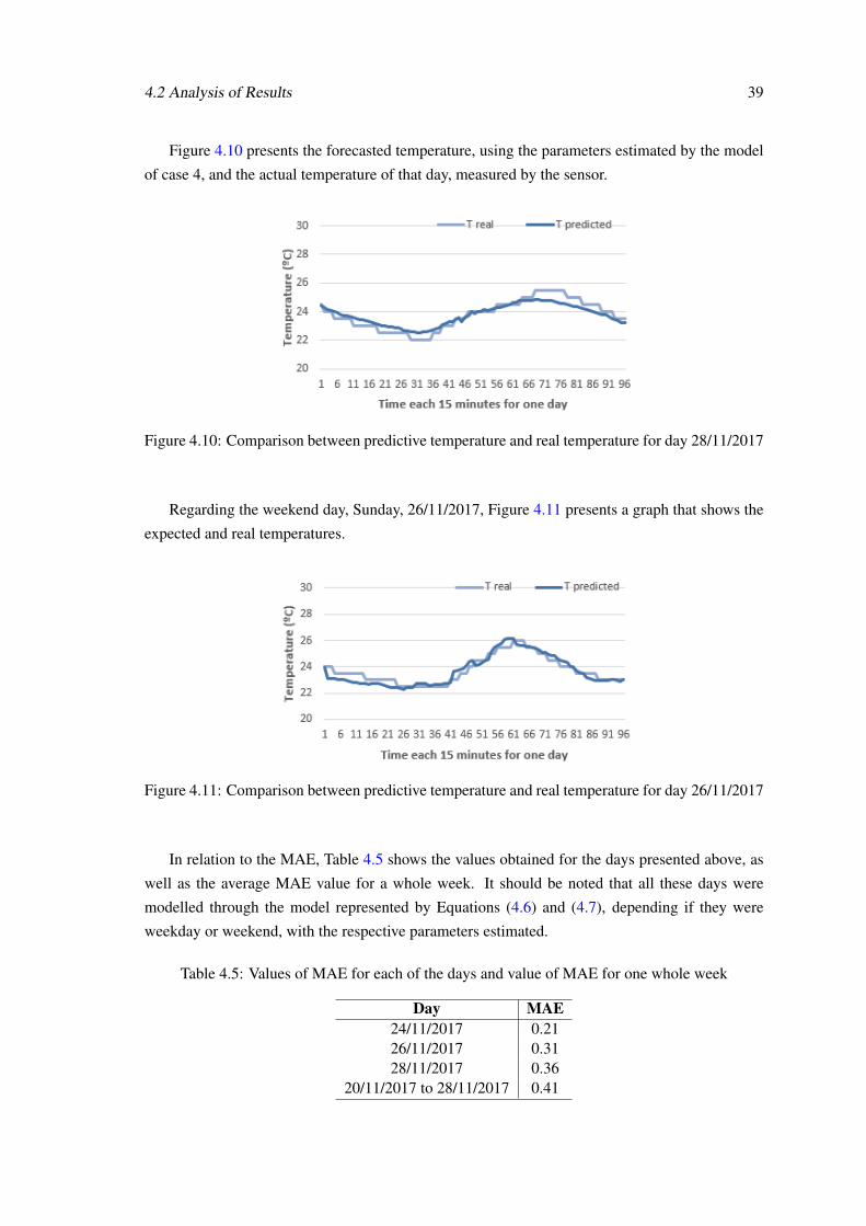
4.2 Analysis of Results 39

Figure 4.10 presents the forecasted temperature, using the parameters estimated by the model

of case 4, and the actual temperature of that day, measured by the sensor.

Figure 4.10: Comparison between predictive temperature and real temperature for day 28/11/2017

Regarding the weekend day, Sunday, 26/11/2017, Figure 4.11 presents a graph that shows the

expected and real temperatures.

Figure 4.11: Comparison between predictive temperature and real temperature for day 26/11/2017

In relation to the MAE, Table 4.5 shows the values obtained for the days presented above, as

well as the average MAE value for a whole week. It should be noted that all these days were

modelled through the model represented by Equations (4.6) and (4.7), depending if they were

weekday or weekend, with the respective parameters estimated.

Table 4.5: Values of MAE for each of the days and value of MAE for one whole week

Day MAE24/11/2017 0.2126/11/2017 0.3128/11/2017 0.36

20/11/2017 to 28/11/2017 0.41

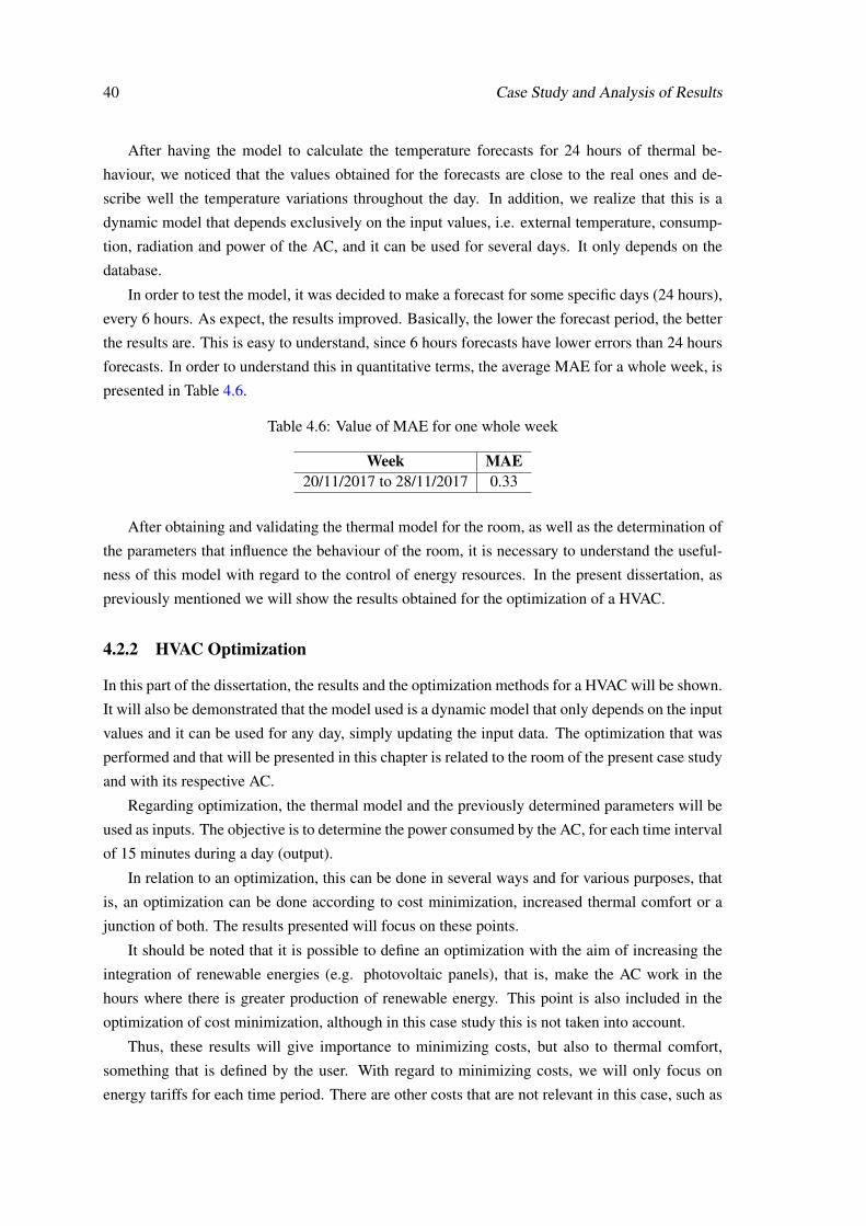
40 Case Study and Analysis of Results

After having the model to calculate the temperature forecasts for 24 hours of thermal be-

haviour, we noticed that the values obtained for the forecasts are close to the real ones and de-

scribe well the temperature variations throughout the day. In addition, we realize that this is a

dynamic model that depends exclusively on the input values, i.e. external temperature, consump-

tion, radiation and power of the AC, and it can be used for several days. It only depends on the

database.

In order to test the model, it was decided to make a forecast for some specific days (24 hours),

every 6 hours. As expect, the results improved. Basically, the lower the forecast period, the better

the results are. This is easy to understand, since 6 hours forecasts have lower errors than 24 hours

forecasts. In order to understand this in quantitative terms, the average MAE for a whole week, is

presented in Table 4.6.

Table 4.6: Value of MAE for one whole week

Week MAE20/11/2017 to 28/11/2017 0.33

After obtaining and validating the thermal model for the room, as well as the determination of

the parameters that influence the behaviour of the room, it is necessary to understand the useful-

ness of this model with regard to the control of energy resources. In the present dissertation, as

previously mentioned we will show the results obtained for the optimization of a HVAC.

4.2.2 HVAC Optimization

In this part of the dissertation, the results and the optimization methods for a HVAC will be shown.

It will also be demonstrated that the model used is a dynamic model that only depends on the input

values and it can be used for any day, simply updating the input data. The optimization that was

performed and that will be presented in this chapter is related to the room of the present case study

and with its respective AC.

Regarding optimization, the thermal model and the previously determined parameters will be

used as inputs. The objective is to determine the power consumed by the AC, for each time interval

of 15 minutes during a day (output).

In relation to an optimization, this can be done in several ways and for various purposes, that

is, an optimization can be done according to cost minimization, increased thermal comfort or a

junction of both. The results presented will focus on these points.

It should be noted that it is possible to define an optimization with the aim of increasing the

integration of renewable energies (e.g. photovoltaic panels), that is, make the AC work in the

hours where there is greater production of renewable energy. This point is also included in the

optimization of cost minimization, although in this case study this is not taken into account.

Thus, these results will give importance to minimizing costs, but also to thermal comfort,

something that is defined by the user. With regard to minimizing costs, we will only focus on

energy tariffs for each time period. There are other costs that are not relevant in this case, such as

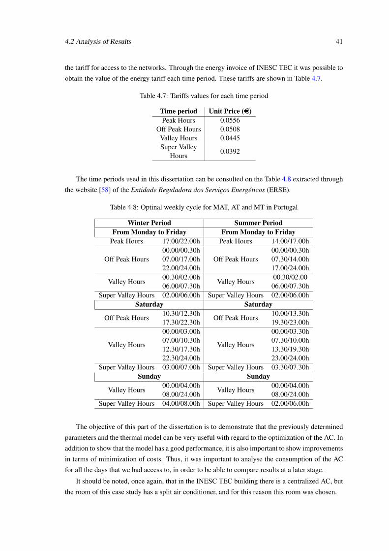
4.2 Analysis of Results 41

the tariff for access to the networks. Through the energy invoice of INESC TEC it was possible to

obtain the value of the energy tariff each time period. These tariffs are shown in Table 4.7.

Table 4.7: Tariffs values for each time period

Time period Unit Price (e)Peak Hours 0.0556

Off Peak Hours 0.0508Valley Hours 0.0445Super Valley

Hours0.0392

The time periods used in this dissertation can be consulted on the Table 4.8 extracted through

the website [58] of the Entidade Reguladora dos Serviços Energéticos (ERSE).

Table 4.8: Optinal weekly cycle for MAT, AT and MT in Portugal

Winter Period Summer PeriodFrom Monday to Friday From Monday to Friday

Peak Hours 17.00/22.00h Peak Hours 14.00/17.00h

Off Peak Hours00.00/00.30h

Off Peak Hours00.00/00.30h

07.00/17.00h 07.30/14.00h22.00/24.00h 17.00/24.00h

Valley Hours00.30/02.00h

Valley Hours00.30/02.00

06.00/07.30h 06.00/07.30hSuper Valley Hours 02.00/06.00h Super Valley Hours 02.00/06.00h

Saturday Saturday

Off Peak Hours10.30/12.30h

Off Peak Hours10.00/13.30h

17.30/22.30h 19.30/23.00h

Valley Hours

00.00/03.00h

Valley Hours

00.00/03.30h07.00/10.30h 07.30/10.00h12.30/17.30h 13.30/19.30h22.30/24.00h 23.00/24.00h

Super Valley Hours 03.00/07.00h Super Valley Hours 03.30/07.30hSunday Sunday

Valley Hours00.00/04.00h

Valley Hours00.00/04.00h

08.00/24.00h 08.00/24.00hSuper Valley Hours 04.00/08.00h Super Valley Hours 02.00/06.00h

The objective of this part of the dissertation is to demonstrate that the previously determined

parameters and the thermal model can be very useful with regard to the optimization of the AC. In

addition to show that the model has a good performance, it is also important to show improvements

in terms of minimization of costs. Thus, it was important to analyse the consumption of the AC

for all the days that we had access to, in order to be able to compare results at a later stage.

It should be noted, once again, that in the INESC TEC building there is a centralized AC, but

the room of this case study has a split air conditioner, and for this reason this room was chosen.

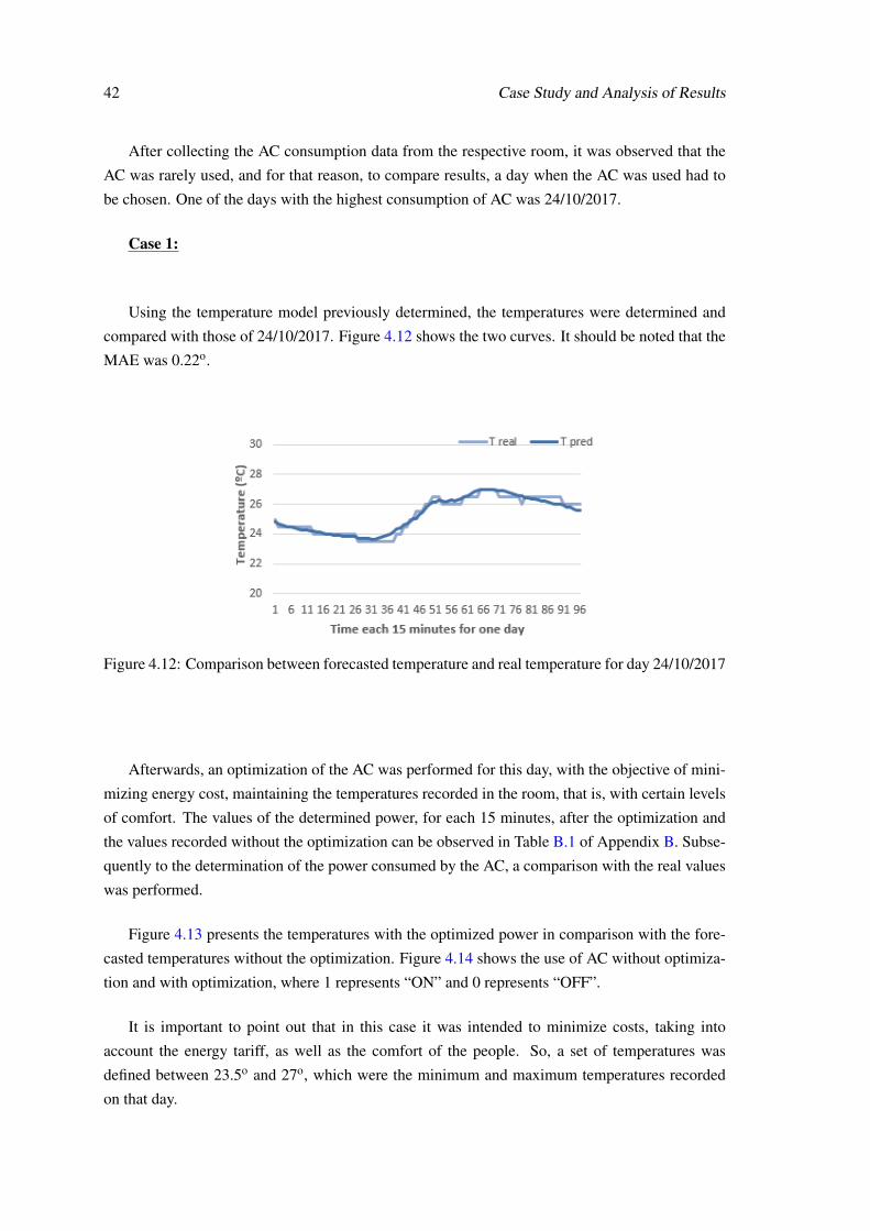
42 Case Study and Analysis of Results

After collecting the AC consumption data from the respective room, it was observed that the

AC was rarely used, and for that reason, to compare results, a day when the AC was used had to

be chosen. One of the days with the highest consumption of AC was 24/10/2017.

Case 1:

Using the temperature model previously determined, the temperatures were determined and

compared with those of 24/10/2017. Figure 4.12 shows the two curves. It should be noted that the

MAE was 0.22o.

Figure 4.12: Comparison between forecasted temperature and real temperature for day 24/10/2017

Afterwards, an optimization of the AC was performed for this day, with the objective of mini-

mizing energy cost, maintaining the temperatures recorded in the room, that is, with certain levels

of comfort. The values of the determined power, for each 15 minutes, after the optimization and

the values recorded without the optimization can be observed in Table B.1 of Appendix B. Subse-

quently to the determination of the power consumed by the AC, a comparison with the real values

was performed.

Figure 4.13 presents the temperatures with the optimized power in comparison with the fore-

casted temperatures without the optimization. Figure 4.14 shows the use of AC without optimiza-

tion and with optimization, where 1 represents “ON” and 0 represents “OFF”.

It is important to point out that in this case it was intended to minimize costs, taking into

account the energy tariff, as well as the comfort of the people. So, a set of temperatures was

defined between 23.5o and 27o, which were the minimum and maximum temperatures recorded

on that day.

4.2 Analysis of Results 43

Figure 4.13: Comparison between predictive temperature with and without optimization for case1

Figure 4.14: AC operation with and without optimization for case1. 1 when AC is On and 0 whenAC is off

The MAE value calculated between the two temperatures was 0.166o. Regarding the consump-

tion, without optimization, the value of the cost obtained for this day was 0.113 e, while with the

optimization the value was 0.083 e, that is, reductions in the order of 26.5% were obtained.

It can be seen that there is an inverse relation between comfort and cost minimization, meaning

that less comfort can lead to higher reductions in energy costs. Two cases will be presented for

another day, 25/10/2017, where the AC was also used.

Case 2 will demonstrate a scenario where the minimization of costs is the focal point, while

case 3, besides the minimization of costs, will focus on the thermal comfort of the users. The

power consumption for every 15 minutes in 24 hours can be found in Table B.2 and Table B.2 of

Appendix B, for case 2 and 3, respectively.

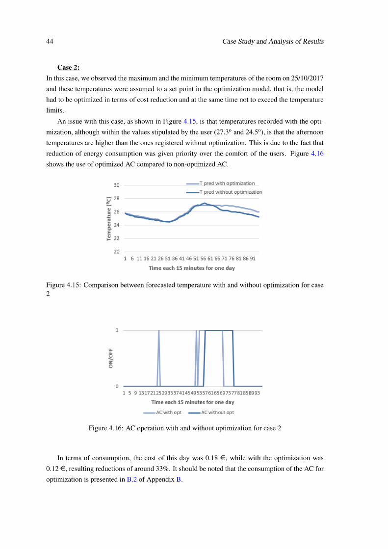
44 Case Study and Analysis of Results

Case 2:In this case, we observed the maximum and the minimum temperatures of the room on 25/10/2017

and these temperatures were assumed to a set point in the optimization model, that is, the model

had to be optimized in terms of cost reduction and at the same time not to exceed the temperature

limits.

An issue with this case, as shown in Figure 4.15, is that temperatures recorded with the opti-

mization, although within the values stipulated by the user (27.3o and 24.5o), is that the afternoon

temperatures are higher than the ones registered without optimization. This is due to the fact that

reduction of energy consumption was given priority over the comfort of the users. Figure 4.16

shows the use of optimized AC compared to non-optimized AC.

Figure 4.15: Comparison between forecasted temperature with and without optimization for case2

Figure 4.16: AC operation with and without optimization for case 2

In terms of consumption, the cost of this day was 0.18 e, while with the optimization was

0.12 e, resulting reductions of around 33%. It should be noted that the consumption of the AC for

optimization is presented in B.2 of Appendix B.

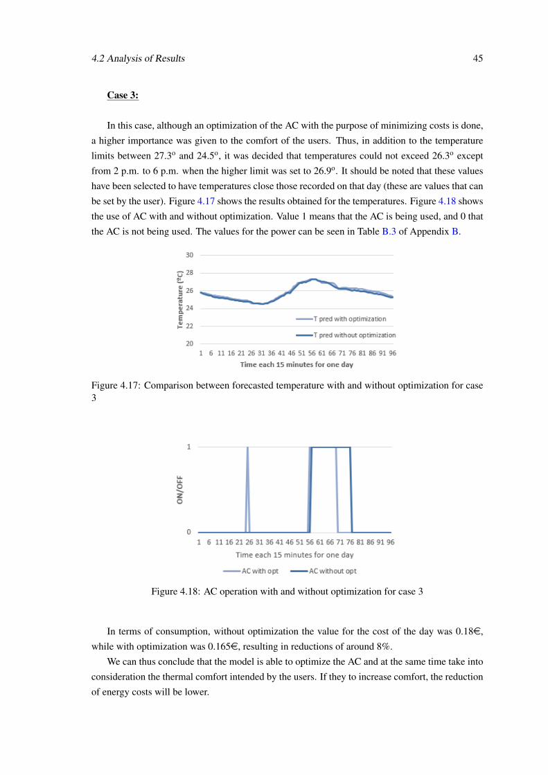
4.2 Analysis of Results 45

Case 3:

In this case, although an optimization of the AC with the purpose of minimizing costs is done,

a higher importance was given to the comfort of the users. Thus, in addition to the temperature

limits between 27.3o and 24.5o, it was decided that temperatures could not exceed 26.3o except

from 2 p.m. to 6 p.m. when the higher limit was set to 26.9o. It should be noted that these values

have been selected to have temperatures close those recorded on that day (these are values that can

be set by the user). Figure 4.17 shows the results obtained for the temperatures. Figure 4.18 shows

the use of AC with and without optimization. Value 1 means that the AC is being used, and 0 that

the AC is not being used. The values for the power can be seen in Table B.3 of Appendix B.

Figure 4.17: Comparison between forecasted temperature with and without optimization for case3

Figure 4.18: AC operation with and without optimization for case 3

In terms of consumption, without optimization the value for the cost of the day was 0.18e,

while with optimization was 0.165e, resulting in reductions of around 8%.

We can thus conclude that the model is able to optimize the AC and at the same time take into

consideration the thermal comfort intended by the users. If they to increase comfort, the reduction

of energy costs will be lower.

46 Case Study and Analysis of Results

In numerical terms, the cost of using the AC is very reduced. This is owed to the centralized

AC of the other rooms of the building, which leads to thermal energy transferred from the adja-

cent rooms, resulting in a little use of the split air conditioner. On the other hand, in terms of

percentages, a significant reduction of energy costs has been achieved, while the desired comforts

levels were maintained. As it can be seen in the figures concerning the use of AC, the optimization

defines the best period to act as well as to at which power should the AC operate to attain a given

temperature.

As in the previous cases the AC is only used for cooling, it was decided to show case 4 where

the AC is used to heat and cool the room during the same day. Thus, the room will maintain a

more or less constant temperature for the whole day, not having a great variation. This means

that a higher importance is given to thermal comfort than to the cost minimization. Even so, the

optimization also takes the thermal comfort into account.

Case 4:

In this case, it is assumed that the users want the temperature for a given day (24/10/2017) to

be always between 24.5o and 25.5o.

Thus, the optimization model receives this temperature setting by the users and determines

the temperatures for the next 24 hours, taking into account the possible minimization in terms of

energy costs. The graph of Figure 4.19 shows the temperature for the respective day after the

optimization and in Figure 4.20 can be observed the behaviour of the AC (when it is heating up

and cooling down the room). The respective power can be found in in Table B.4 of Appendix B.

Figure 4.19: Temperature with optimization for case 4

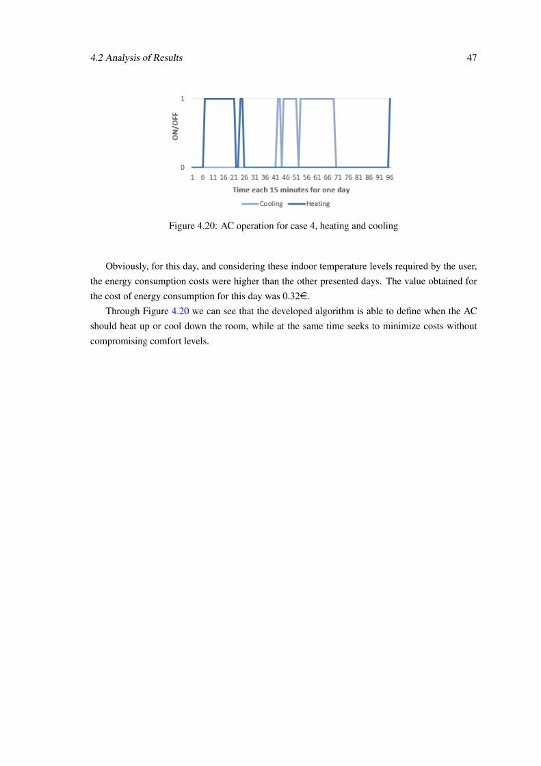
4.2 Analysis of Results 47

Figure 4.20: AC operation for case 4, heating and cooling

Obviously, for this day, and considering these indoor temperature levels required by the user,

the energy consumption costs were higher than the other presented days. The value obtained for

the cost of energy consumption for this day was 0.32e.

Through Figure 4.20 we can see that the developed algorithm is able to define when the AC

should heat up or cool down the room, while at the same time seeks to minimize costs without

compromising comfort levels.

48 Case Study and Analysis of Results

Chapter 5

Conclusion, Main Achievements andFuture Work

5.1 Conclusion and Main Achievements

This chapter presents the final considerations after the developed work, as well as the analysis of

the results obtained. Firstly, it can be concluded that the objectives were fulfilled with success.

Throughout the work developed, and through the application of the various models, it was pos-

sible to put into practice the theory studied, deepening knowledge, through the difficulties and

challenges encountered in each stage of application of the model.

This study had the purpose of deepening the knowledge around online estimation of thermal

parameters through non-linear optimization. The objective was to estimate the parameters and, af-

terwards, use them to model the thermal behaviour of the room and to optimize energy equipment.

In the present case, the optimization of an AC was performed through an objective function.

By analysing the obtained results, it is possible to conclude that the thermal behaviour of the

room was successfully modelled using several determined parameters. It can also be concluded

that even when all the parameters of a room are not known a priori (e.g. resistance or thermal

capacity), these can be obtained through the grey box approach using the least-squares method. It

should be noted that in addition to the methods used, the data collection over the period of about a

month was essential for the determination of all parameters.

Regarding the thermal model of the room, for the determination of variables and respective

gains (parameters), approximately one month was used for training data, in order to obtain the

best possible results. With less training data, the results would not have been as close to reality as

they effectively were. In average terms, for one week, the value obtained for the MAE was 0.4o

and on a specific day was obtained a value of around 0.2o. In addition, although the results were

satisfactory and represented well the thermal behaviour of the room, it should be taken into account

that the data used for training and testing corresponded to the month of October and November.

The model was not tested for days of other seasons, such as Summer or Spring due to the lack of

49

50 Conclusion, Main Achievements and Future Work

data. It is perceptible that some gains such as radiation have a greater impact in some seasons than

others.

Regarding the optimization model, despite some initial obstacles, due to the fact that the use of

the AC of the room of the study case is small, it was possible to demonstrate the implementation

of the model and its good performance, due to the fact that it is a model that only depends on

the inputs from the database. In economic terms, there has been a significant improvement in

terms of cost reduction, while taking into account user comfort levels. The optimization of the

AC was carried out considering the reduction of costs, and the comfort levels established by the

user. Regarding the obtained values, reductions of the cost of energy consumption between 25

and 33% were achieved. An important aspect that was observed was that giving more importance

to user comfort, with more limited temperature restrictions, will lead to higher energy costs, even

considering that the optimization problem tries to minimize them at all times. Consequently, lower

reductions in energy costs (8%) were achieved on a specific day, where the comfort level of the

users was increased.

As a conclusion, the work developed may have a significant impact on society, with regard to

smart buildings and the active load control, since it contributes to minimize energy consumption

without compromising the comfort level of the users and, consequently, to reduce CO2 emissions.

This study demonstrates that the methodology used can be implemented in any corporate or resi-

dential building. Thus, the main achievement of this dissertation was the development of a method

that can be easily implemented in an energy management system (BEMS or HEMS), acting as a

demand response service in homes or in corporate buildings, with the purpose of reducing energy

costs. It allows controlling energy resources in an effective way, making buildings “smarter”.

Furthermore, it is clear that there are opportunities for improving the energy efficiency of

buildings, especially regarding loads management. In addition, it was noted that weather forecasts

had a big influence on the room’s temperature. Thus, it is concluded that meteorological forecasts

play a key role in the management of the loads and in the performance of demand response services

involving air conditioning and other heating/cooling equipment.

Finally, it is concluded that distributed energy resources, such as HVAC systems, can easily

reduce/increase consumption over certain periods, so as to contribute to a better functioning of the

overall energy system.

5.2 Future Work

This work presents a proposal for the determination of the parameters that model the thermal

behaviour of a room, in order to optimize an AC. The strategy implemented has shown that it is

possible to reduce the energy costs of a building. However, it would be interesting to continue

studying possible improvements in the energy efficiency of a building, with many directions to be

explored, in order to improve the methods presented in this dissertation.

A possible improvement in the model the accurate modelling of the thermal gains from other

rooms, that is, to study the energy exchanges between adjacent rooms by creating multiple thermal

5.2 Future Work 51

models and characterising their interaction. This approach can be replicated for several rooms and

scaled up to represent an entire building. Additionally, it would be interesting to perform this same

study on other seasons and understand the behaviour of the variables that influence the indoor room

temperature.

Additionally, it would be interesting to put into practice the model developed and to use a MPC

in a real installation where the model would be constantly working, updating inputs and forecasts

every 15 minutes to prove its economic potential.

In addition, to evaluate the model in conjunction with renewable energy sources (e.g. pho-

tovoltaic and wind power) would be very interesting, as the uncertainty associated with these

resources is high. This would contribute evaluate the performance of the optimization model in

more adverse conditions.

52 Conclusion, Main Achievements and Future Work

References

[1] Yi Kai Juan, Peng Gao, and Jie Wang. A hybrid decision support system for sustainableoffice building renovation and energy performance improvement. Energy and Buildings,42(3):290–297, 2010. doi:10.1016/j.enbuild.2009.09.006.

[2] Hai Xiang Zhao and Frédéric Magoulès. A review on the prediction of building energyconsumption. Renewable and Sustainable Energy Reviews, 16(6):3586–3592, 2012. URL:http://dx.doi.org/10.1016/j.rser.2012.02.049, doi:10.1016/j.rser.2012.02.049.

[3] BCSD Portugal. Eficiência Energética em Edifícios. 2007.

[4] Biao Sun, PB Luh, QS Jia, Ziyan Jiang, Fulin Wang, and Chen Song. Building En-ergy Management: Integrated Control of Active and Passive Heating, Cooling, Light-ing, Shading, and Ventilation Systems. Ieeexplore.Ieee.Org, pages 1–15, 2012. URL:http://ieeexplore.ieee.org/xpls/abs_all.jsp?arnumber=6256761.

[5] Bingnan Jiang and Yunsi Fei. Energy Procedia Dynamic Residential Demand Response andDistributed Generation Management in Smart Microgrid with Hierarchical Agents. EnergyProcedia, 12:76–90, 2011. URL: http://dx.doi.org/10.1016/j.egypro.2011.10.012, doi:10.1016/j.egypro.2011.10.012.

[6] Miguel (INESC TEC) Heleno. Provision of advanced ancillary services through demandside integration. PhD thesis, 2015.

[7] Miguel Heleno, Manuel A. Matos, J. A. Pecas Lopes, and J. P. Iria. Estimating the flexibleresidential load using appliances availability. Proceedings of the 2014 IEEE 8th InternationalPower Engineering and Optimization Conference, PEOCO 2014, (March):352–357, 2014.doi:10.1109/PEOCO.2014.6814453.

[8] Hassan Farhangi. The path of the smart grid. IEEE Power and Energy Magazine, 8(1):18–28,2010. arXiv:10, doi:10.1109/MPE.2009.934876.

[9] M. Hatami, G. Domairry, and S. N. Mirzababaei. Experimental investigation of preparing andusing the H2O based nanofluids in the heating process of HVAC system model. InternationalJournal of Hydrogen Energy, 42(12):7820–7825, 2017. URL: http://dx.doi.org/10.1016/j.ijhydene.2016.12.104, doi:10.1016/j.ijhydene.2016.12.104.

[10] M. Schicktanz and T. Núñez. Modelling of an adsorption chiller for dynamic system sim-ulation. International Journal of Refrigeration, 32(4):588–595, 2009. doi:10.1016/j.ijrefrig.2009.02.011.

53

54 REFERENCES

[11] Soma Shekara Sreenadh Reddy Depuru, Lingfeng Wang, and Vijay Devabhaktuni. Smartmeters for power grid: Challenges, issues, advantages and status. Renewable and Sustain-able Energy Reviews, 15(6):2736–2742, 2011. URL: http://dx.doi.org/10.1016/j.rser.2011.02.039, doi:10.1016/j.rser.2011.02.039.

[12] S. Aman, Y. Simmhan, and V.K. Prasanna. Energy management systems: stateof the art and emerging trends. IEEE Communications Magazine, 51(1):114–119,2013. URL: http://ieeexplore.ieee.org/ielx5/35/6400427/06400447.pdf?tp=&arnumber=6400447&isnumber=6400427%5Cnhttp://ieeexplore.ieee.org/xpls/abs_all.jsp?arnumber=6400447,doi:10.1109/MCOM.2013.6400447.

[13] D. Y. Raghavendra Nagesh, J. V. Vamshi Krishna, and S. S. Tulasiram. A real-time architec-ture for smart energy management. Innovative Smart Grid Technologies Conference, ISGT2010, pages 1–4, 2010. doi:10.1109/ISGT.2010.5434771.

[14] E.M.G. Rodrigues, R. Godina, E. Pouresmaeil, J.R. Ferreira, and J.P.S.Catalão. Domestic appliances energy optimization with model predictivecontrol. Energy Conversion and Management, 142:402–413, 2017. URL:http://linkinghub.elsevier.com/retrieve/pii/S0196890417302728,doi:10.1016/j.enconman.2017.03.061.

[15] Yongmin Yan, Jin Zhou, Yaolin Lin, Wei Yang, Ping Wang, and Guoqiang Zhang. Adap-tive optimal control model for building cooling and heating sources. Energy and Buildings,40(8):1394–1401, 2008. doi:10.1016/j.enbuild.2008.01.003.

[16] Bing Dong. Non-linear optimal controller design for building HVAC sys-tems. 2010 IEEE International Conference on Control Applications, (1):210–215, 2010. URL: http://ieeexplore.ieee.org/document/5611260/,doi:10.1109/CCA.2010.5611260.

[17] S.Joe Qin and Thomas A. Badgwell. A survey of industrial model predictive control technol-ogy. Control Engineering Practice, 11(7):733–764, 2003. arXiv:arXiv:1402.6991v1,doi:10.1016/S0967-0661(02)00186-7.

[18] Weijie Mai and C. Y. Chung. Economic MPC of Aggregating Commercial Buildings forProviding Flexible Power Reserve. IEEE Transactions on Power Systems, 30(5):2685–2694,2015. doi:10.1109/TPWRS.2014.2365615.

[19] Massimo Fiorentini, Josh Wall, Zhenjun Ma, Julio H. Braslavsky, and Paul Cooper. Hybridmodel predictive control of a residential HVAC system with on-site thermal energy genera-tion and storage. Applied Energy, 187:465–479, 2017. URL: http://dx.doi.org/10.1016/j.apenergy.2016.11.041, doi:10.1016/j.apenergy.2016.11.041.

[20] Sorin C. Bengea, Anthony D. Kelman, Francesco Borrelli, Russell Taylor, and SatishNarayanan. Implementation of model predictive control for an HVAC system in a mid-size commercial building. HVAC&R Research, 20(1):121–135, 2014. URL: http://www.tandfonline.com/doi/abs/10.1080/10789669.2013.834781, doi:10.1080/10789669.2013.834781.

[21] Christofer Sundstr, Daniel Jung, and Anders Blom. Analysis of Optimal Energy Managementin Smart Homes Using MPC. pages 2066–2071, 2016.

REFERENCES 55

[22] Yi Zong, Georg Martin Böning, Rui Mirra Santos, Shi You, Junjie Hu, and Xue Han.Challenges of implementing economic model predictive control strategy for buildings in-teracting with smart energy systems. Applied Thermal Engineering, 114:1476–1486,2017. URL: http://dx.doi.org/10.1016/j.applthermaleng.2016.11.141,doi:10.1016/j.applthermaleng.2016.11.141.

[23] Yudong Ma, Garrett Anderson, and Francesco Borrelli. A Distributed Predictive ControlApproach to Building Temperature Regulation. American Control Conference, pages 2089–2094, 2011. doi:10.1109/ACC.2011.5991549.

[24] David Sturzenegger, Dimitrios Gyalistras, Vito Semeraro, Manfred Morari, andRoy S. Smith. BRCM Matlab Toolbox: Model generation for model pre-dictive building control. 2014 American Control Conference, pages 1063–1069,2014. URL: http://ieeexplore.ieee.org/lpdocs/epic03/wrapper.htm?arnumber=6858967, doi:10.1109/ACC.2014.6858967.

[25] Qiang Zhou, Shengwei Wang, Xinhua Xu, and Fu Xiao. A grey-box model of next-daybuilding thermal load prediction for energy-efficient control. International journal of energyresearch, -(-):–, 2008. arXiv:arXiv:1011.1669v3, doi:10.1002/er.

[26] J A Crabb, N Murdoch, and J M Penman. A simplified thermal response model. Build-ing Services Engineering Research and Technology, 8(1):13–19, 1987. URL: http://journals.sagepub.com/doi/10.1177/014362448700800104, doi:10.1177/014362448700800104.

[27] Srinivas Katipamula and Michael R Brambley. Review Article : Methods for Fault Detection, Diagnostics , and Prognostics for Building Systems — A Review , Part II Methods forFault Detection , Diagnostics , and Prognostics for Building Systems — A Review , Part II.9669(May 2015):37–41, 2005. doi:10.1080/10789669.2005.10391133.

[28] Edris Pouresmaeil, Juan Miguel Gonzalez, and Claudio a Canizares. Devel-opment of a Smart Residential Load Simulator for Energy Management inSmart Grids. Ieee Transactions on Power System, pages 1–8, 2014. URL:https://uwaterloo.ca/power-energy-systems-group/sites/ca.power-energy-systems-group/files/uploads/files/srls.pdf.

[29] Herie Park, Marie Ruellan, Adrien Bouvet, Eric Monmasson, and Rachid Bennacer. Thermalparameter identification of simplified building model with electric appliance. Proceedingof the International Conference on Electrical Power Quality and Utilisation, EPQU, pages499–504, 2011. arXiv:0402594v3, doi:10.1109/EPQU.2011.6128822.

[30] Zhenyu Yang, Xiaoli Li, C. P. Bowers, T. Schnier, Ke Tang, and Xin Yao. An Effi-cient Evolutionary Approach to Parameter Identification in a Building Thermal Model.IEEE Transactions on Systems, Man, and Cybernetics, Part C (Applications and Reviews),42(6):957–969, 2012. URL: http://ieeexplore.ieee.org/document/6105579/,doi:10.1109/TSMCC.2011.2174983.

[31] Fatima Amara, Kodjo Agbossou, Alben Cardenas, Yves Dubé, and Sousso Kelouwani.Comparison and Simulation of Building Thermal Models for Effective Energy Man-agement. Smart Grid and Renewable Energy, 06(04):95–112, 2015. URL: http://www.scirp.org/journal/doi.aspx?DOI=10.4236/sgre.2015.64009,doi:10.4236/sgre.2015.64009.

56 REFERENCES

[32] Mehdi Maasoumy, Barzin Moridian, and Meysam Razmara. ONLINE SIMULTANEOUSSTATE ESTIMATION AND PARAMETER ADAPTATION FOR BUILDING PREDIC-TIVE CONTROL. 201. URL: http://sinberbest.berkeley.edu/.

[33] Clara Verhelst. Model Predictive Control of Ground Coupled Heat Pump Systems for OfficeBuildings. Number April. 2012.

[34] Fernanda De Oliveira Resende. “ Contributions for MicroGrids Dynamic Modelling andOperation ”. page 293, 2007.

[35] Clara Verhelst, Filip Logist, Jan Van Impe, and Lieve Helsen. Study of the optimal controlproblem formulation for modulating air-to-water heat pumps connected to a residential floorheating system. Energy and Buildings, 45:43–53, 2012. URL: http://dx.doi.org/10.1016/j.enbuild.2011.10.015, doi:10.1016/j.enbuild.2011.10.015.

[36] Jean Lebrun. Simulation of a Hvac System With the Help of an Engineering Equation Solver.Seventh International IBPSA Conference, Rio de Janerio, Brazil, August 13-15, 2001, pages1119–1126, 2001.

[37] F. Déqué, F. Ollivier, and A. Poblador. Grey boxes used to represent buildings with a min-imum number of geometric and thermal parameters. Energy and Buildings, 31(1):29–35,2000. doi:10.1016/S0378-7788(98)00074-7.

[38] Kun Deng, Siddharth Goyal, Prabir Barooah, and Prashant G. Mehta. Structure-preserving model reduction of nonlinear building thermal models. Automatica,50(4):1188–1195, 2014. URL: http://linkinghub.elsevier.com/retrieve/pii/S0005109814000478, doi:10.1016/j.automatica.2014.02.009.

[39] Jan Široký, Frauke Oldewurtel, Jirí Cigler, and Samuel Prívara. Experimental analysis ofmodel predictive control for an energy efficient building heating system. Applied Energy,88(9):3079–3087, 2011. doi:10.1016/j.apenergy.2011.03.009.

[40] Samuel Prívara, Jan Široký, Lukáš Ferkl, and Jirí Cigler. Model predictive control of abuilding heating system: The first experience. Energy and Buildings, 43(2-3):564–572, 2011.doi:10.1016/j.enbuild.2010.10.022.

[41] a Molina, A Gabaldon, J.a Fuentes, and C. Alvarez. Implementation and assessment ofphysically based electrical load models: Application to direct load control residential pro-grammes. Generation, Transmission and Distribution, IEE Proceedings-, 150:61–66, 2003.URL: http://bibliotecavirtual.ups.edu.ec:2065/ielx5/2195/26841/01193672.pdf?tp=&arnumber=1193672&isnumber=26841%5Cnhttp://bibliotecavirtual.ups.edu.ec:2065/xpl/articleDetails.jsp?tp=&arnumber=1193672&queryText=Implementation+and+assessment+of+physically+based+, doi:10.1049/ip-gid:20020750.

[42] C. F. Walker and J. L. Pokoski. Residential Load Shape Modeling Based on Customer Behav-ior. IEEE Power Engineering Review, PER-5(7):34, 1985. doi:10.1109/MPER.1985.5528462.

[43] Friederich Kupzog and Charlotte Roesener. A closer Look on Load Manage-ment. 2007 5th IEEE International Conference on Industrial Informatics, 2:1151–1156, 2007. URL: http://ieeexplore.ieee.org/lpdocs/epic03/wrapper.htm?arnumber=4384893, doi:10.1109/INDIN.2007.4384893.

REFERENCES 57

[44] D Bargiotas and JD Birdwell. Residential air conditioner dynamic model for direct loadcontrol. Power Delivery, IEEE Transactions . . . , 3(4):2119–2126, 1988. URL: http://ieeexplore.ieee.org/xpls/abs_all.jsp?arnumber=194024.

[45] Cristian Perfumo, Ernesto Kofman, Julio H. Braslavsky, and John K. Ward. Loadmanagement: Model-based control of aggregate power for populations of ther-mostatically controlled loads. Energy Conversion and Management, 55:36–48,2012. URL: http://dx.doi.org/10.1016/j.enconman.2011.10.019, doi:10.1016/j.enconman.2011.10.019.

[46] José Iria, Filipe Soares, and Manuel Matos. Optimal supply and demand bid-ding strategy for an aggregator of small prosumers. Applied Energy, (June):1–12,2017. URL: http://dx.doi.org/10.1016/j.apenergy.2017.09.002, doi:10.1016/j.apenergy.2017.09.002.

[47] Duncan S. Callaway. Tapping the energy storage potential in electric loads to deliver loadfollowing and regulation, with application to wind energy. Energy Conversion and Manage-ment, 50(5):1389–1400, 2009. URL: http://dx.doi.org/10.1016/j.enconman.2008.12.012, doi:10.1016/j.enconman.2008.12.012.

[48] Madhur Behl, Truong X. Nghiem, and Rahul Mangharam. IMpACT: Inverse model accu-racy and control performance toolbox for buildings. IEEE International Conference on Au-tomation Science and Engineering, 2014-Janua:1109–1114, 2014. doi:10.1109/CoASE.2014.6899464.

[49] Lee Holland, Student Member, H Bora Karayaka, Senior Member, Martin L Tanaka, andAaron Ball. An Empirical Method for Estimating Thermal System Parameters Based onOperating Data in Smart Grids. pages 0–4, 2014. doi:10.1109/ISGT.2014.6816457.

[50] Sami El-Ferik, Syed A. Hussain, and Fouad M. Al-Sunni. Identification and weather sensi-tivity of physically based model of residential air-conditioners for direct load control: A casestudy. Energy and Buildings, 38(8):997–1005, 2006. doi:10.1016/j.enbuild.2005.11.010.

[51] P Radecki and B Hencey. Online Building Thermal Parameter Estimation via UnscentedKalman Filtering. 2012 American Control Conference (ACC), pages 3056–3062, 2012. doi:10.1109/acc.2012.6315699.

[52] About Pyomo. URL: http://www.pyomo.org/about/.

[53] IPOPT: Python Package Index. URL: https://pypi.python.org/pypi/ipopt.

[54] Related Commercial Resources. NONRESIDENTIAL COOLING AND HEATING. 2009.

[55] GLPK - GNU Linear Programming Kit. URL: https://www.gnu.org/software/glpk/.

[56] MeteoGalicia - predición xeral para Galicia. URL: http://www.meteogalicia.gal/web/index.action.

[57] EasyLog EL-USB-1-LCD. URL: https://www.lascarelectronics.com/easylog-data-logger-el-usb-1-lcd/.

58 REFERENCES

[58] Portal ERSE - Ciclo semanal opcional para os consumidores em MAT, AT e MT em PortugalContinental. URL: http://www.erse.pt/pt/electricidade/tarifaseprecos/periodoshorarios/Paginas/CiclopcionalosconsumidoresMATATMT.aspx.

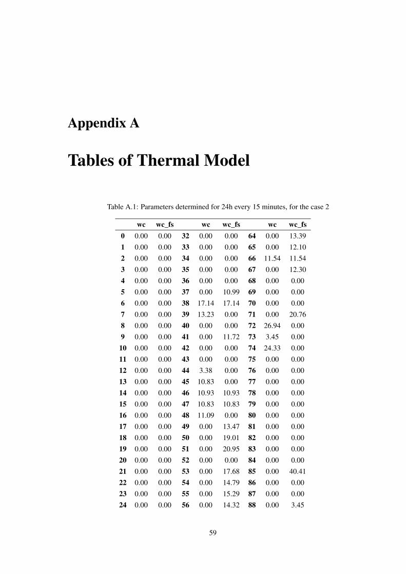
Appendix A

Tables of Thermal Model

Table A.1: Parameters determined for 24h every 15 minutes, for the case 2

wc wc_fs wc wc_fs wc wc_fs0 0.00 0.00 32 0.00 0.00 64 0.00 13.39

1 0.00 0.00 33 0.00 0.00 65 0.00 12.10

2 0.00 0.00 34 0.00 0.00 66 11.54 11.54

3 0.00 0.00 35 0.00 0.00 67 0.00 12.30

4 0.00 0.00 36 0.00 0.00 68 0.00 0.00

5 0.00 0.00 37 0.00 10.99 69 0.00 0.00

6 0.00 0.00 38 17.14 17.14 70 0.00 0.00

7 0.00 0.00 39 13.23 0.00 71 0.00 20.76

8 0.00 0.00 40 0.00 0.00 72 26.94 0.00

9 0.00 0.00 41 0.00 11.72 73 3.45 0.00

10 0.00 0.00 42 0.00 0.00 74 24.33 0.00

11 0.00 0.00 43 0.00 0.00 75 0.00 0.00

12 0.00 0.00 44 3.38 0.00 76 0.00 0.00

13 0.00 0.00 45 10.83 0.00 77 0.00 0.00

14 0.00 0.00 46 10.93 10.93 78 0.00 0.00

15 0.00 0.00 47 10.83 10.83 79 0.00 0.00

16 0.00 0.00 48 11.09 0.00 80 0.00 0.00

17 0.00 0.00 49 0.00 13.47 81 0.00 0.00

18 0.00 0.00 50 0.00 19.01 82 0.00 0.00

19 0.00 0.00 51 0.00 20.95 83 0.00 0.00

20 0.00 0.00 52 0.00 0.00 84 0.00 0.00

21 0.00 0.00 53 0.00 17.68 85 0.00 40.41

22 0.00 0.00 54 0.00 14.79 86 0.00 0.00

23 0.00 0.00 55 0.00 15.29 87 0.00 0.00

24 0.00 0.00 56 0.00 14.32 88 0.00 3.45

59

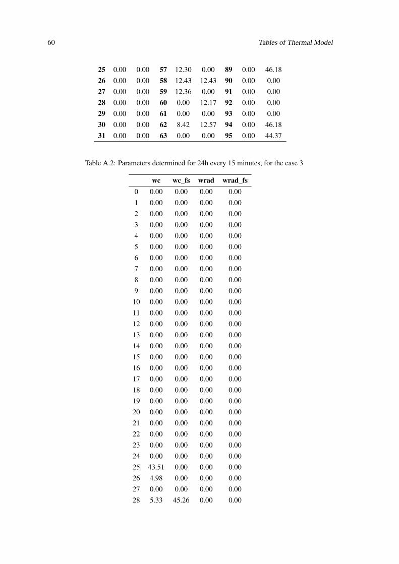
60 Tables of Thermal Model

25 0.00 0.00 57 12.30 0.00 89 0.00 46.18

26 0.00 0.00 58 12.43 12.43 90 0.00 0.00

27 0.00 0.00 59 12.36 0.00 91 0.00 0.00

28 0.00 0.00 60 0.00 12.17 92 0.00 0.00

29 0.00 0.00 61 0.00 0.00 93 0.00 0.00

30 0.00 0.00 62 8.42 12.57 94 0.00 46.18

31 0.00 0.00 63 0.00 0.00 95 0.00 44.37

Table A.2: Parameters determined for 24h every 15 minutes, for the case 3

wc wc_fs wrad wrad_fs0 0.00 0.00 0.00 0.00

1 0.00 0.00 0.00 0.00

2 0.00 0.00 0.00 0.00

3 0.00 0.00 0.00 0.00

4 0.00 0.00 0.00 0.00

5 0.00 0.00 0.00 0.00

6 0.00 0.00 0.00 0.00

7 0.00 0.00 0.00 0.00

8 0.00 0.00 0.00 0.00

9 0.00 0.00 0.00 0.00

10 0.00 0.00 0.00 0.00

11 0.00 0.00 0.00 0.00

12 0.00 0.00 0.00 0.00

13 0.00 0.00 0.00 0.00

14 0.00 0.00 0.00 0.00

15 0.00 0.00 0.00 0.00

16 0.00 0.00 0.00 0.00

17 0.00 0.00 0.00 0.00

18 0.00 0.00 0.00 0.00

19 0.00 0.00 0.00 0.00

20 0.00 0.00 0.00 0.00

21 0.00 0.00 0.00 0.00

22 0.00 0.00 0.00 0.00

23 0.00 0.00 0.00 0.00

24 0.00 0.00 0.00 0.00

25 43.51 0.00 0.00 0.00

26 4.98 0.00 0.00 0.00

27 0.00 0.00 0.00 0.00

28 5.33 45.26 0.00 0.00

Tables of Thermal Model 61

29 0.00 0.00 0.00 0.00

30 0.00 0.00 0.00 0.00

31 0.00 0.00 0.00 0.00

32 0.00 0.00 0.00 0.00

33 0.00 0.00 0.00 0.00

34 0.00 0.00 0.00 0.00

35 0.00 0.00 0.00 0.00

36 0.00 0.00 0.00 0.00

37 17.14 0.00 0.00 0.00

38 17.14 0.73 0.00 0.00

39 0.00 0.00 0.00 0.00

40 0.06 0.00 65.29 71.65

41 0.00 0.00 13.87 11.11

42 0.00 0.00 23.82 7.30

43 0.00 0.00 65.63 50.44

44 0.00 0.00 0.00 2.53

45 0.00 0.00 0.30 11.30

46 0.00 0.00 21.15 5.62

47 5.16 0.00 0.00 33.60

48 11.09 0.00 0.00 0.00

49 0.00 0.00 0.00 0.00

50 0.00 0.00 0.00 0.00

51 0.00 0.00 0.00 0.00

52 1.21 0.00 8.62 26.57

53 0.00 0.00 0.00 7.95

54 0.13 0.00 0.00 1.54

55 13.95 0.00 0.00 0.00

56 8.10 0.00 0.00 11.82

57 0.00 0.00 0.00 0.00

58 0.00 0.00 0.00 0.00

59 0.00 0.00 0.00 0.00

60 0.00 0.00 29.38 0.00

61 0.00 0.00 9.42 0.00

62 0.00 0.00 2.89 0.00

63 0.00 0.00 0.00 0.00

64 0.00 7.33 0.00 0.00

65 0.00 12.10 0.00 0.00

66 2.68 0.00 0.00 0.00

67 7.97 0.00 0.00 0.00

68 0.00 0.00 0.00 0.00

62 Tables of Thermal Model

69 0.00 0.00 0.00 0.00

70 0.00 0.00 0.00 0.00

71 0.00 0.00 0.00 0.00

72 0.00 0.00 0.00 0.00

73 0.00 0.00 0.00 0.00

74 0.00 0.00 0.00 0.00

75 0.00 0.00 0.00 0.00

76 0.00 0.00 0.00 0.00

77 0.00 0.00 0.00 0.00

78 0.00 0.00 0.00 0.00

79 0.00 0.00 0.00 0.00

80 0.00 0.00 0.00 0.00

81 0.00 0.00 0.00 0.00

82 0.00 0.00 0.00 0.00

83 0.00 0.00 0.00 0.00

84 0.00 0.00 0.00 0.00

85 0.00 12.67 0.00 0.00

86 0.00 0.00 0.00 0.00

87 0.00 0.00 0.00 0.00

88 0.00 0.00 0.00 0.00

89 0.00 46.18 0.00 0.00

90 0.00 0.00 0.00 0.00

91 0.00 0.00 0.00 0.00

92 0.00 0.00 0.00 0.00

93 0.00 0.00 0.00 0.00

94 0.00 46.18 0.00 0.00

95 0.00 44.37 0.00 0.00

Table A.3: Parameters determined for 24h every 15 minutes, for the case 4

wc wc_fs wrad wrad_fs wextra wextra_fs0 0.00 0.00 0.00 0.00 -2.40 -15.70

1 0.00 0.00 0.00 0.00 -0.32 0.54

2 0.00 0.00 0.00 0.00 0.53 1.44

3 0.00 0.00 0.00 0.00 -0.35 0.53

4 0.00 0.00 0.00 0.00 0.47 0.69

5 0.00 0.00 0.00 0.00 -0.85 1.39

6 0.00 0.00 0.00 0.00 -0.42 0.49

7 0.00 0.00 0.00 0.00 0.88 -0.45

8 0.00 0.00 0.00 0.00 0.06 -0.43

Tables of Thermal Model 63

9 0.00 0.00 0.00 0.00 0.94 0.48

10 0.00 0.00 0.00 0.00 0.49 1.37

11 0.00 0.00 0.00 0.00 0.49 0.48

12 0.00 0.00 0.00 0.00 0.53 1.41

13 0.00 0.00 0.00 0.00 0.52 -0.41

14 0.00 14.87 0.00 0.00 -0.36 0.50

15 0.00 0.00 0.00 0.00 0.51 1.38

16 0.00 0.00 0.00 0.00 0.08 1.44

17 0.00 0.00 0.00 0.00 0.50 0.50

18 0.00 0.00 0.00 0.00 0.07 -0.41

19 0.00 0.00 0.00 0.00 0.93 0.49

20 0.00 0.00 0.00 0.00 0.07 0.51

21 0.00 0.00 0.00 0.00 1.38 0.51

22 0.00 0.00 0.00 0.00 0.94 1.41

23 0.00 0.00 0.00 0.00 0.93 0.51

24 0.00 0.00 0.00 0.00 0.51 0.52

25 0.00 14.48 0.00 0.00 -1.23 1.44

26 0.00 0.00 0.00 0.00 0.93 1.44

27 0.00 0.00 0.00 0.00 0.93 1.41

28 0.00 45.26 0.00 0.00 1.37 0.55

29 0.00 0.00 0.00 0.00 0.07 1.45

30 0.00 0.00 0.00 0.00 0.93 1.44

31 0.00 0.00 0.00 0.00 2.24 1.45

32 0.00 0.00 0.00 0.00 1.80 -0.37

33 0.00 0.00 0.00 0.00 3.12 1.44

34 0.00 0.00 0.00 0.00 2.70 3.28

35 0.00 0.00 0.00 0.00 3.15 1.47

36 0.00 0.00 0.00 0.00 3.94 2.28

37 0.00 0.00 0.00 0.00 5.27 2.29

38 0.00 0.00 0.00 0.00 3.54 2.32

39 0.00 0.00 0.00 0.00 4.86 3.24

40 0.00 0.00 41.71 101.30 -2.75 -7.01

41 0.00 0.00 0.00 11.82 4.32 0.14

42 0.00 0.00 4.61 8.01 4.73 2.16

43 0.00 0.00 76.25 47.60 -10.62 -9.20

44 0.00 0.00 0.00 2.48 6.84 4.74

45 0.00 0.00 0.00 11.68 4.21 3.85

46 0.00 0.00 0.00 6.00 8.16 2.03

47 0.00 0.00 44.14 36.81 -10.61 -22.54

48 0.00 0.00 0.00 0.00 5.42 3.73

64 Tables of Thermal Model

49 0.00 0.00 0.00 0.00 1.52 3.75

50 0.00 0.00 0.00 0.00 3.71 5.60

51 0.00 0.00 0.00 0.00 -0.61 3.79

52 0.00 0.00 0.00 25.09 2.42 2.81

53 0.00 0.00 0.00 8.18 3.20 3.74

54 0.00 0.00 0.00 6.07 2.42 2.84

55 0.00 0.00 0.00 0.64 1.27 3.77

56 0.00 0.00 0.00 12.85 2.75 2.82

57 0.00 0.00 0.00 2.64 2.57 1.93

58 0.00 0.00 0.00 0.00 3.60 1.94

59 0.00 0.00 0.00 0.00 3.40 1.04

60 0.00 0.00 10.07 2.02 0.21 -9.13

61 0.00 0.00 4.72 0.00 1.92 -0.15

62 0.00 0.00 3.21 0.00 1.16 1.96

63 0.00 0.00 3.17 0.00 0.83 -0.79

64 0.00 0.00 0.00 0.00 1.46 1.11

65 0.00 12.10 0.00 0.00 1.03 -0.43

66 6.19 0.00 0.00 0.00 -3.24 -0.72

67 0.00 0.00 0.00 0.00 0.51 -0.74

68 0.00 0.00 0.00 0.00 0.18 -2.43

69 0.00 0.00 0.00 0.00 1.47 1.21

70 0.00 0.00 0.00 0.00 1.47 -1.54

71 0.00 0.00 0.00 0.00 0.99 -0.64

72 0.00 0.00 0.00 0.00 -0.32 1.32

73 0.00 0.00 0.00 0.00 -0.32 -2.35

74 0.00 0.00 0.00 0.00 0.10 -1.46

75 0.00 0.00 0.00 0.00 1.37 -0.55

76 0.00 0.00 0.00 0.00 0.57 0.46

77 7.76 0.00 0.00 0.00 -2.31 -4.75

78 0.00 0.00 0.00 0.00 0.09 0.44

79 0.00 0.00 0.00 0.00 0.51 -3.56

80 0.00 0.00 0.00 0.00 0.57 -2.62

81 0.00 0.00 0.00 0.00 -0.34 0.50

82 0.00 3.33 0.00 0.00 0.08 -5.87

83 0.00 0.00 0.00 0.00 0.07 0.48

84 0.00 0.00 0.00 0.00 0.11 -0.40

85 0.00 0.00 0.00 0.00 0.10 1.06

86 0.00 0.00 0.00 0.00 0.09 0.51

87 0.00 0.00 0.00 0.00 0.52 1.42

88 0.00 0.00 0.00 0.00 0.98 1.45

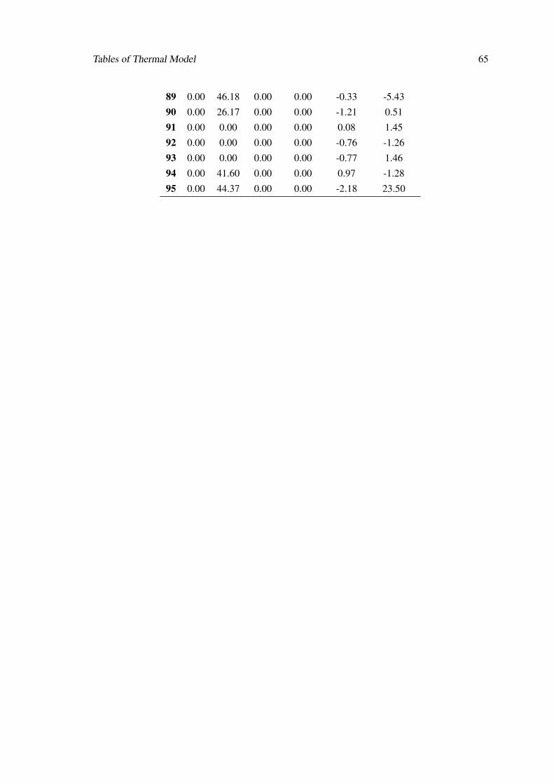
Tables of Thermal Model 65

89 0.00 46.18 0.00 0.00 -0.33 -5.43

90 0.00 26.17 0.00 0.00 -1.21 0.51

91 0.00 0.00 0.00 0.00 0.08 1.45

92 0.00 0.00 0.00 0.00 -0.76 -1.26

93 0.00 0.00 0.00 0.00 -0.77 1.46

94 0.00 41.60 0.00 0.00 0.97 -1.28

95 0.00 44.37 0.00 0.00 -2.18 23.50

66 Tables of Thermal Model

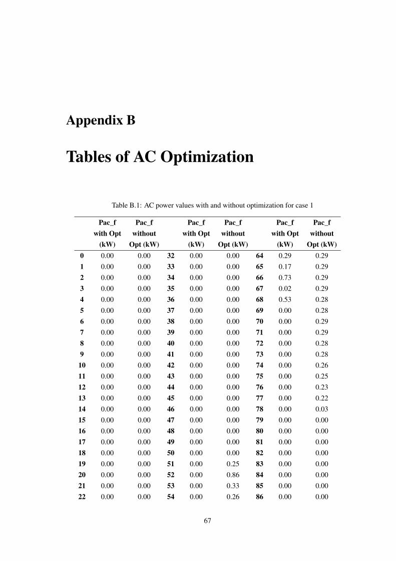
Appendix B

Tables of AC Optimization

Table B.1: AC power values with and without optimization for case 1

Pac_fwith Opt

(kW)

Pac_fwithout

Opt (kW)

Pac_fwith Opt

(kW)

Pac_fwithout

Opt (kW)

Pac_fwith Opt

(kW)

Pac_fwithout

Opt (kW)0 0.00 0.00 32 0.00 0.00 64 0.29 0.29

1 0.00 0.00 33 0.00 0.00 65 0.17 0.29

2 0.00 0.00 34 0.00 0.00 66 0.73 0.29

3 0.00 0.00 35 0.00 0.00 67 0.02 0.29

4 0.00 0.00 36 0.00 0.00 68 0.53 0.28

5 0.00 0.00 37 0.00 0.00 69 0.00 0.28

6 0.00 0.00 38 0.00 0.00 70 0.00 0.29

7 0.00 0.00 39 0.00 0.00 71 0.00 0.29

8 0.00 0.00 40 0.00 0.00 72 0.00 0.28

9 0.00 0.00 41 0.00 0.00 73 0.00 0.28

10 0.00 0.00 42 0.00 0.00 74 0.00 0.26

11 0.00 0.00 43 0.00 0.00 75 0.00 0.25

12 0.00 0.00 44 0.00 0.00 76 0.00 0.23

13 0.00 0.00 45 0.00 0.00 77 0.00 0.22

14 0.00 0.00 46 0.00 0.00 78 0.00 0.03

15 0.00 0.00 47 0.00 0.00 79 0.00 0.00

16 0.00 0.00 48 0.00 0.00 80 0.00 0.00

17 0.00 0.00 49 0.00 0.00 81 0.00 0.00

18 0.00 0.00 50 0.00 0.00 82 0.00 0.00

19 0.00 0.00 51 0.00 0.25 83 0.00 0.00

20 0.00 0.00 52 0.00 0.86 84 0.00 0.00

21 0.00 0.00 53 0.00 0.33 85 0.00 0.00

22 0.00 0.00 54 0.00 0.26 86 0.00 0.00

67

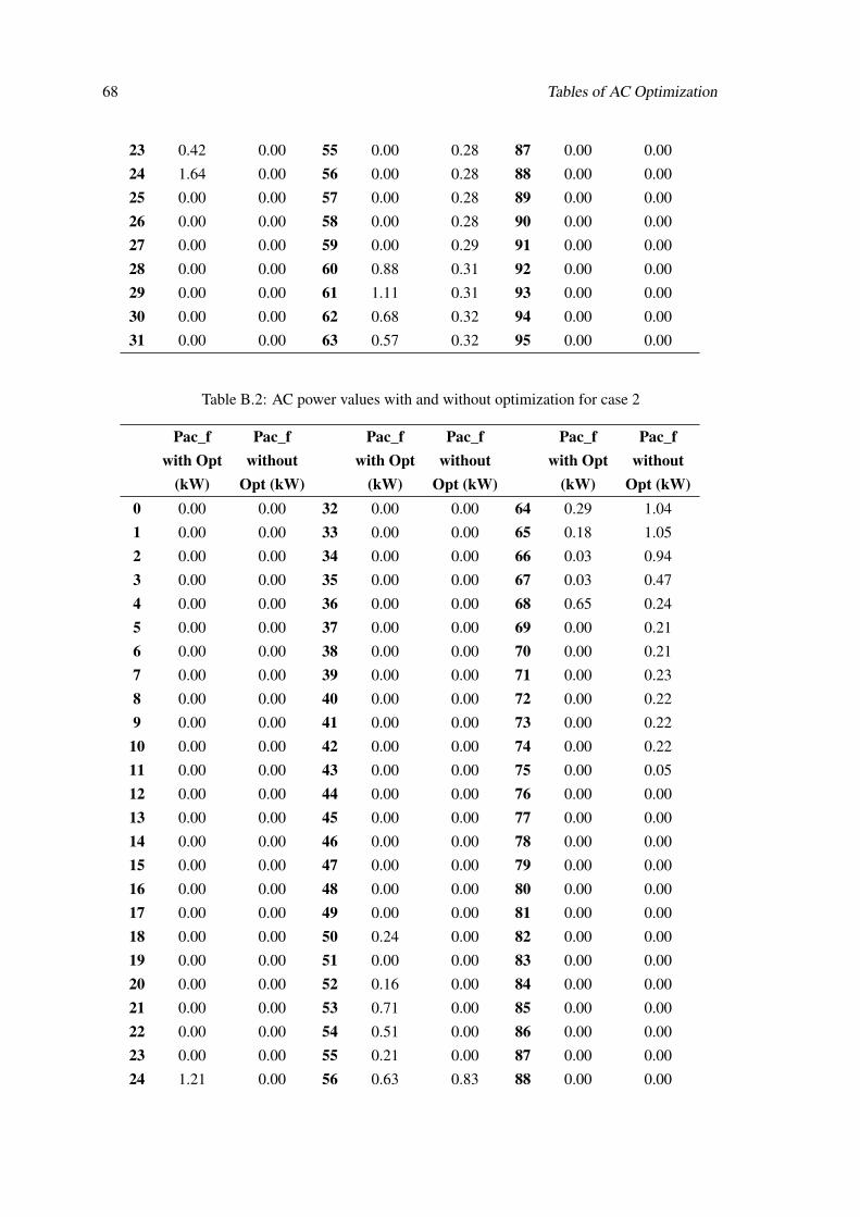
68 Tables of AC Optimization

23 0.42 0.00 55 0.00 0.28 87 0.00 0.00

24 1.64 0.00 56 0.00 0.28 88 0.00 0.00

25 0.00 0.00 57 0.00 0.28 89 0.00 0.00

26 0.00 0.00 58 0.00 0.28 90 0.00 0.00

27 0.00 0.00 59 0.00 0.29 91 0.00 0.00

28 0.00 0.00 60 0.88 0.31 92 0.00 0.00

29 0.00 0.00 61 1.11 0.31 93 0.00 0.00

30 0.00 0.00 62 0.68 0.32 94 0.00 0.00

31 0.00 0.00 63 0.57 0.32 95 0.00 0.00

Table B.2: AC power values with and without optimization for case 2

Pac_fwith Opt

(kW)

Pac_fwithout

Opt (kW)

Pac_fwith Opt

(kW)

Pac_fwithout

Opt (kW)

Pac_fwith Opt

(kW)

Pac_fwithout

Opt (kW)0 0.00 0.00 32 0.00 0.00 64 0.29 1.04

1 0.00 0.00 33 0.00 0.00 65 0.18 1.05

2 0.00 0.00 34 0.00 0.00 66 0.03 0.94

3 0.00 0.00 35 0.00 0.00 67 0.03 0.47

4 0.00 0.00 36 0.00 0.00 68 0.65 0.24

5 0.00 0.00 37 0.00 0.00 69 0.00 0.21

6 0.00 0.00 38 0.00 0.00 70 0.00 0.21

7 0.00 0.00 39 0.00 0.00 71 0.00 0.23

8 0.00 0.00 40 0.00 0.00 72 0.00 0.22

9 0.00 0.00 41 0.00 0.00 73 0.00 0.22

10 0.00 0.00 42 0.00 0.00 74 0.00 0.22

11 0.00 0.00 43 0.00 0.00 75 0.00 0.05

12 0.00 0.00 44 0.00 0.00 76 0.00 0.00

13 0.00 0.00 45 0.00 0.00 77 0.00 0.00

14 0.00 0.00 46 0.00 0.00 78 0.00 0.00

15 0.00 0.00 47 0.00 0.00 79 0.00 0.00

16 0.00 0.00 48 0.00 0.00 80 0.00 0.00

17 0.00 0.00 49 0.00 0.00 81 0.00 0.00

18 0.00 0.00 50 0.24 0.00 82 0.00 0.00

19 0.00 0.00 51 0.00 0.00 83 0.00 0.00

20 0.00 0.00 52 0.16 0.00 84 0.00 0.00

21 0.00 0.00 53 0.71 0.00 85 0.00 0.00

22 0.00 0.00 54 0.51 0.00 86 0.00 0.00

23 0.00 0.00 55 0.21 0.00 87 0.00 0.00

24 1.21 0.00 56 0.63 0.83 88 0.00 0.00

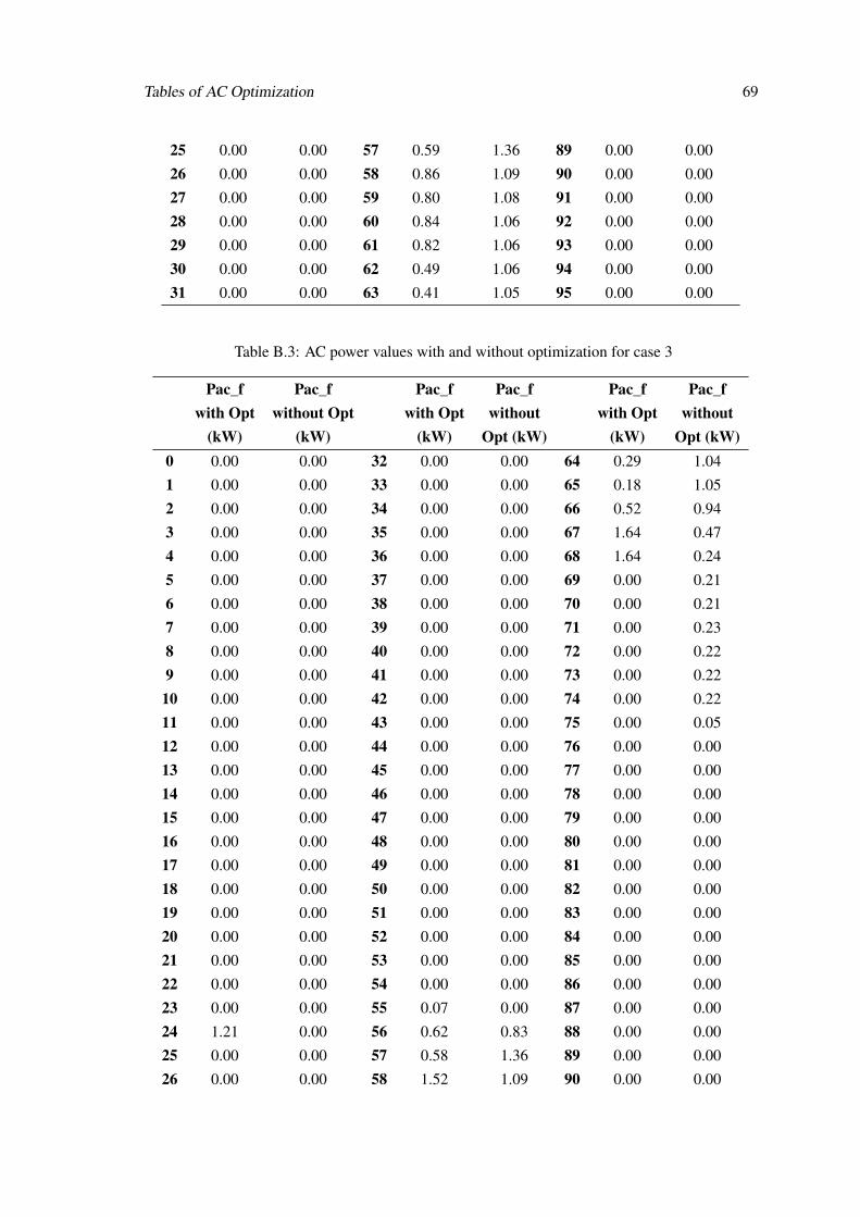
Tables of AC Optimization 69

25 0.00 0.00 57 0.59 1.36 89 0.00 0.00

26 0.00 0.00 58 0.86 1.09 90 0.00 0.00

27 0.00 0.00 59 0.80 1.08 91 0.00 0.00

28 0.00 0.00 60 0.84 1.06 92 0.00 0.00

29 0.00 0.00 61 0.82 1.06 93 0.00 0.00

30 0.00 0.00 62 0.49 1.06 94 0.00 0.00

31 0.00 0.00 63 0.41 1.05 95 0.00 0.00

Table B.3: AC power values with and without optimization for case 3

Pac_fwith Opt

(kW)

Pac_fwithout Opt

(kW)

Pac_fwith Opt

(kW)

Pac_fwithout

Opt (kW)

Pac_fwith Opt

(kW)

Pac_fwithout

Opt (kW)0 0.00 0.00 32 0.00 0.00 64 0.29 1.04

1 0.00 0.00 33 0.00 0.00 65 0.18 1.05

2 0.00 0.00 34 0.00 0.00 66 0.52 0.94

3 0.00 0.00 35 0.00 0.00 67 1.64 0.47

4 0.00 0.00 36 0.00 0.00 68 1.64 0.24

5 0.00 0.00 37 0.00 0.00 69 0.00 0.21

6 0.00 0.00 38 0.00 0.00 70 0.00 0.21

7 0.00 0.00 39 0.00 0.00 71 0.00 0.23

8 0.00 0.00 40 0.00 0.00 72 0.00 0.22

9 0.00 0.00 41 0.00 0.00 73 0.00 0.22

10 0.00 0.00 42 0.00 0.00 74 0.00 0.22

11 0.00 0.00 43 0.00 0.00 75 0.00 0.05

12 0.00 0.00 44 0.00 0.00 76 0.00 0.00

13 0.00 0.00 45 0.00 0.00 77 0.00 0.00

14 0.00 0.00 46 0.00 0.00 78 0.00 0.00

15 0.00 0.00 47 0.00 0.00 79 0.00 0.00

16 0.00 0.00 48 0.00 0.00 80 0.00 0.00

17 0.00 0.00 49 0.00 0.00 81 0.00 0.00

18 0.00 0.00 50 0.00 0.00 82 0.00 0.00

19 0.00 0.00 51 0.00 0.00 83 0.00 0.00

20 0.00 0.00 52 0.00 0.00 84 0.00 0.00

21 0.00 0.00 53 0.00 0.00 85 0.00 0.00

22 0.00 0.00 54 0.00 0.00 86 0.00 0.00

23 0.00 0.00 55 0.07 0.00 87 0.00 0.00

24 1.21 0.00 56 0.62 0.83 88 0.00 0.00

25 0.00 0.00 57 0.58 1.36 89 0.00 0.00

26 0.00 0.00 58 1.52 1.09 90 0.00 0.00

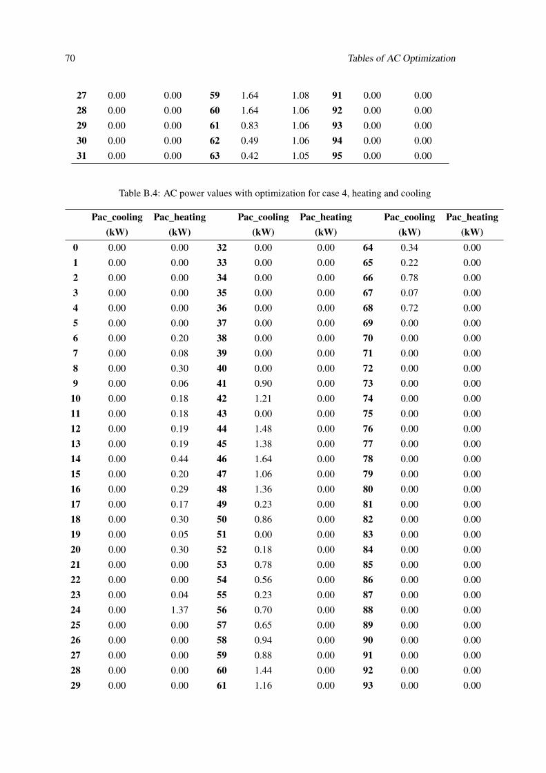
70 Tables of AC Optimization

27 0.00 0.00 59 1.64 1.08 91 0.00 0.00

28 0.00 0.00 60 1.64 1.06 92 0.00 0.00

29 0.00 0.00 61 0.83 1.06 93 0.00 0.00

30 0.00 0.00 62 0.49 1.06 94 0.00 0.00

31 0.00 0.00 63 0.42 1.05 95 0.00 0.00

Table B.4: AC power values with optimization for case 4, heating and cooling

Pac_cooling(kW)

Pac_heating(kW)

Pac_cooling(kW)

Pac_heating(kW)

Pac_cooling(kW)

Pac_heating(kW)

0 0.00 0.00 32 0.00 0.00 64 0.34 0.00

1 0.00 0.00 33 0.00 0.00 65 0.22 0.00

2 0.00 0.00 34 0.00 0.00 66 0.78 0.00

3 0.00 0.00 35 0.00 0.00 67 0.07 0.00

4 0.00 0.00 36 0.00 0.00 68 0.72 0.00

5 0.00 0.00 37 0.00 0.00 69 0.00 0.00

6 0.00 0.20 38 0.00 0.00 70 0.00 0.00

7 0.00 0.08 39 0.00 0.00 71 0.00 0.00

8 0.00 0.30 40 0.00 0.00 72 0.00 0.00

9 0.00 0.06 41 0.90 0.00 73 0.00 0.00

10 0.00 0.18 42 1.21 0.00 74 0.00 0.00

11 0.00 0.18 43 0.00 0.00 75 0.00 0.00

12 0.00 0.19 44 1.48 0.00 76 0.00 0.00

13 0.00 0.19 45 1.38 0.00 77 0.00 0.00

14 0.00 0.44 46 1.64 0.00 78 0.00 0.00

15 0.00 0.20 47 1.06 0.00 79 0.00 0.00

16 0.00 0.29 48 1.36 0.00 80 0.00 0.00

17 0.00 0.17 49 0.23 0.00 81 0.00 0.00

18 0.00 0.30 50 0.86 0.00 82 0.00 0.00

19 0.00 0.05 51 0.00 0.00 83 0.00 0.00

20 0.00 0.30 52 0.18 0.00 84 0.00 0.00

21 0.00 0.00 53 0.78 0.00 85 0.00 0.00

22 0.00 0.00 54 0.56 0.00 86 0.00 0.00

23 0.00 0.04 55 0.23 0.00 87 0.00 0.00

24 0.00 1.37 56 0.70 0.00 88 0.00 0.00

25 0.00 0.00 57 0.65 0.00 89 0.00 0.00

26 0.00 0.00 58 0.94 0.00 90 0.00 0.00

27 0.00 0.00 59 0.88 0.00 91 0.00 0.00

28 0.00 0.00 60 1.44 0.00 92 0.00 0.00

29 0.00 0.00 61 1.16 0.00 93 0.00 0.00

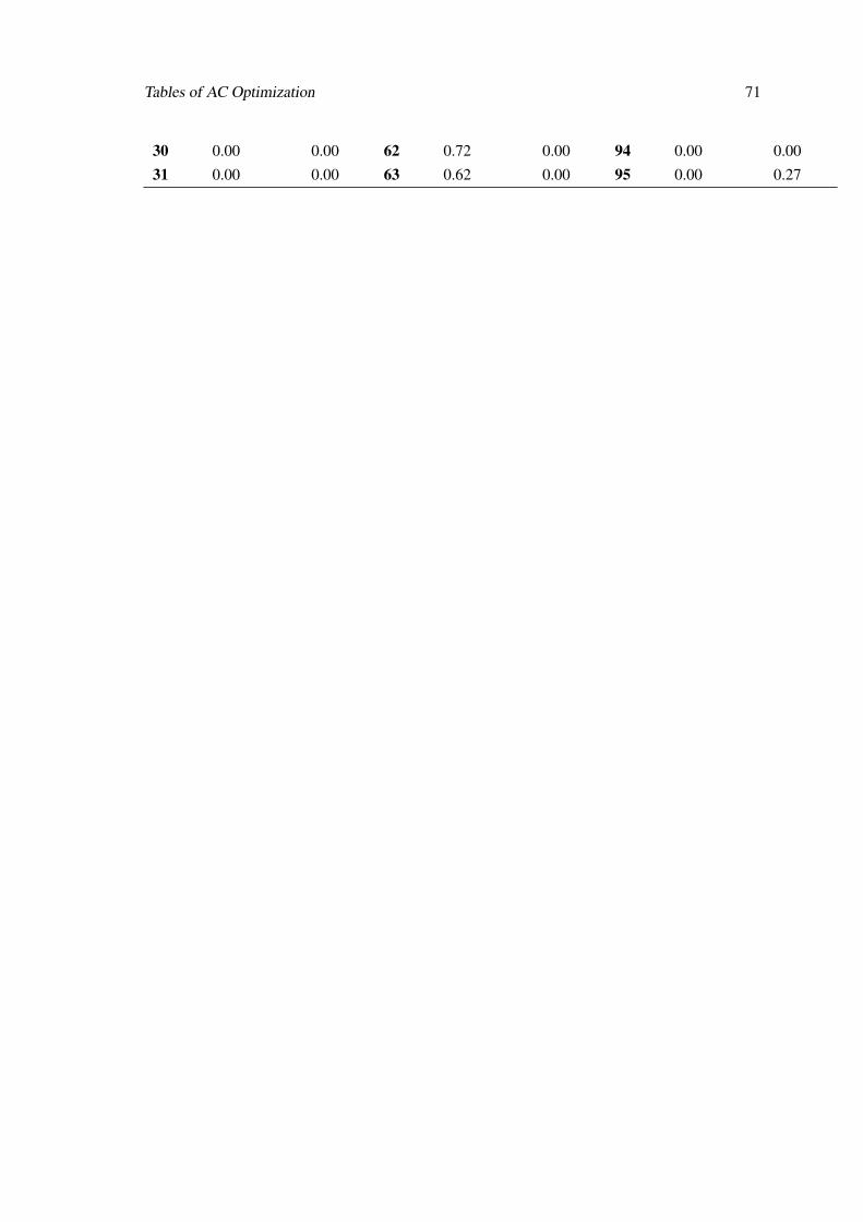
Tables of AC Optimization 71

30 0.00 0.00 62 0.72 0.00 94 0.00 0.00

31 0.00 0.00 63 0.62 0.00 95 0.00 0.27