Information Sciences 220 (2013) 22–33

Contents lists available at SciVerse ScienceDirect

Information Sciences

journal homepage: www.elsevier .com/locate / ins

Online extraction of main linear trends for nonlineartime-varying processes

Ahmad Kalhor a,⇑, Babak N. Araabi a,b, Caro Lucas a,b

a Control and Intelligent Processing Center of Excellence, School of Electrical and Computer Engineering, University of Tehran, Tehran, Iranb School of Cognitive Sciences, Institute for Research in Fundamental Sciences (IPM), Tehran, Iran

a r t i c l e i n f o a b s t r a c t

Article history:Available online 26 June 2012

Keywords:Main linear trendOnline clusteringTemporal behaviorAdaptive linear modelElectrical load time series

0020-0255/$ - see front matter � 2012 Elsevier Inchttp://dx.doi.org/10.1016/j.ins.2012.06.022

⇑ Corresponding author. Address: School of ElectrTel.: +98 21 8863 0024; fax: +98 21 8863 3029; cel

E-mail addresses: akalhor@ut.ac.ir (A. Kalhor), ar1 The Eq. (1) can be considered as a wide definitio

states the high-dimensional shape of the rules is the tvalidity regions.

Linear trends of a time-varying process include useful and insight data about its temporalbehaviors. In this paper, we introduce an approach for extracting the main linear trends ofa nonlinear time-varying process. In this approach, originally, an adaptive linear model isutilized to estimate the temporal-linear trends of the process. Then, by using a suitable dis-tance index, an online clustering algorithm has been developed to classify the estimatedlinear trends. Considering the mean and the number of members for each cluster, main lin-ear trends are extracted for the process. Through an illustrative example, the methodologyof the proposed approach in extracting main linear trends is explained and its capability isshown. Also, through two case studies –electrical load time series and pH neutralizationprocess– the application of the proposed method in studying temporal behaviors of pro-cesses like stability, changing rate, oscillation and characteristics of transient states areexplained.

� 2012 Elsevier Inc. All rights reserved.

1. Introduction

Studying temporal behaviors of real-time processes such as stability, changing rate, oscillation and transient state isimportant in many engineering and scientific fields [11,2]. There are some nonparametric statistical tools for time seriesanalysis [27,3]; however, temporal behaviors of nonlinear processes are often studied through parametric linear and nonlin-ear models. Although linear models, due to the available temporal and frequency analyzing tools, are much easier to use,they do not have the required flexible structure to study nonlinear and complex cases. Nonlinear models, which are identi-fied as Local Linear Models (LLMs), can supply both simplicity and flexibility to the analysis complex nonlinear processes.First type Takagi Sugeno (TS) fuzzy system forms a large applicable family of LLMs-based nonlinear models [32,35,38]. ATS fuzzy model consists of a set of rules as follows:

IF x is Ai THEN yi ¼ zThi i 2 f1;2; . . . ;Mg ð1Þ

where x 2 Rn is the n-dimensional input vector, yi 2 R is the ith local output, hi 2 Rn+1 is linear parameters of the ith LLM,zT = [xT 1], and Ai is the ith fuzzy set for x, where the related Membership Function (MF) is shown as Ai(x).1 Temporal behav-iors of a process, which is identified by a TS fuzzy model, can be analyzed by extracting its dominant fuzzy rule. For example, if

. All rights reserved.

ical and Computer Engineering, University of Tehran, P.O. Box 14395/515, Tehran 1439957131, Iran.l: +98 912 380 8140.aabi@ut.ac.ir (B.N. Araabi), lucas@ut.ac.ir (C. Lucas).n of the initial TS model introduced by Takagi and Sugeno. Indeed, we have eased the constraint which-norm of single one-dimensional fuzzy sets. This allows one to identify linear sub-models in more flexible

A. Kalhor et al. / Information Sciences 220 (2013) 22–33 23

for a specific time interval, Ai� ðxÞ is much larger than other MFs, one can talk about the temporal behavior of correspondingprocess, with respect to the linear model: yi� ¼ zThi� .

To identify a TS fuzzy model, different techniques have been introduced. Clustering methods have been used as a generalapproach to identify a TS fuzzy model in both offline and online methods: [1,4–6,8,9,17,21,22,24,29,39]. Parameter adapta-tion techniques are widely used as well [20,34,30]. Evolutionary methods and Genetic Algorithms are also utilized to identifyand optimize TS fuzzy models [36,18,13,12].

The type of offline or online identification methods of TS fuzzy models are important to evaluate the validity of theextracting linear trends. Offline identified TS fuzzy models cannot be applied to extract linear trends and analyze behaviorof time-varying processes. In other words, many regimes and process states cannot be practically included into the trainingdata set, but those states close to them could well appear during the process run [15]. To analyze such processes, many adap-tive fuzzy models have been introduced and developed during last decade. Evolving Fuzzy System (EFS) may be used as ageneral term for those fuzzy models and learning methods that try to exploit the interpolation ability, structural flexibilityand interpretability of fuzzy systems in adaptive learning [7]. There are two particularly influential works in this area of re-search [21,6]. Kasabov proposes an adaptive online learning algorithm as a dynamic evolving neural–fuzzy inference system(DENFIS) in [21]. In this algorithm, fuzzy rules are generated using maximum distance clustering approach, which is used topartition the input space. Angelov and Filev introduce an online identification approach for the TS model in [6], where evolv-ing clustering method along with a concept of potential is used to define the antecedent parts of the rules. This approach hasbeen modified and extended in [4,5]. In [26], to evolve a specific form of TS Fuzzy Model, Lughofer suggests to use a modifiedversion of vector quantization for new rule generation. In [23], an online identification of neural–fuzzy model based on indi-rect fuzzy clustering is proposed, and in [24], an agile nonlinear model called ‘‘Adaptive Habitually Linear and TransientlyNonlinear Model’’ (AHLTNM) is introduced to follow an uncertain and fast-varying process.

Although evolving models can be used to analyze existing behavior of a process, they are not necessarily suitable to ana-lyze and study former behaviors. In an evolving model, parameters and the structure may be changed to adapt to new behav-iors of a process. Consequently, some parts of the model, which are associated with former behaviors, are lost.

In this paper, we introduce a capable tool to extract main linear trends of a nonlinear time-varying process. First temporallinear trends of a nonlinear process is estimated and clustered adaptively. Then, main linear trends are extracted from clus-ters. It is shown that this strategy does not have drawbacks of TS fuzzy models; it can directly extract main linear trends oftime-varying processes without having challenges which exist in TS-based identification.

The rest of the paper is organized as follows: Section 2 introduces an adaptive linear model to estimate temporal lineartrends of a process. In Section 3, an online clustering algorithm is proposed to classify the estimating trends. In Section 4,through an illustrative example, the methodology and superiority of the proposed approach are explained; also, to studytemporal behaviors, the proposed approach is applied to two practical case studies: electrical load time series and pH neu-tralization process modeling. Finally the paper is concluded in Section 5.

2. Estimation of temporal linear trends

Here, a constraint on time-varying processes is imposed and then an approach to extract their temporal linear trendsthrough an adaptive linear model is introduced.

2.1. A constraint imposed on a time-varying process

It is supposed that a time-varying process can be approximated as a temporal linear model or equally a temporal lineartrend at each time.

yt ¼ zTt ht zT

t ¼ ½xTt 1�

kDt;tþ1k 6 d; Dt;tþ1 ¼ htþ1 � htð2Þ

where yt is the scalar output of the process at t; xt 2 Rn and ht 2 Rn+1 denote the input vector and linear parameters, respec-tively. Also, Dt,t+1 is an (n + 1)-dimensional vector, which denotes variations of the linear parameters, while the input datachanges from xt to xt+1; the norm of Dt,t+1is bounded by d. One can compute d as maximum norm of Dt,t+1 for a long workingduration of the system. It should be noted that the sampling rate is an important factor to change the d value.

With respect to the imposed constraints on the process, it is reasonable to state that kDt,t+1k can be negligible where theprocess operates in one of its linear trends and it increases where the process switches softly from a linear trend to anothertrend. The soft switching between two linear trends can be interpreted with respect to considered sensitivity to separate thelinear trends. In reality, the soft switching in a system can be interpreted by an expert.

2.2. Estimation of temporal linear trends through an adaptive linear model

With respect to the imposed constraint on the process in Section 2.1, an adaptive linear model is a fitting model to followthe variations of the process. In this case, temporal linear trends of the process can be estimated as parameters of the adap-

24 A. Kalhor et al. / Information Sciences 220 (2013) 22–33

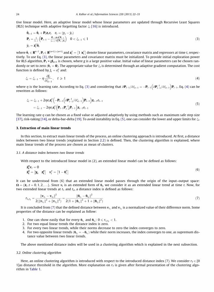
tive linear model. Here, an adaptive linear model whose linear parameters are updated through Recursive Least Squares(RLS) technique with adaptive forgetting factor nt [16] is introduced.

htþ1 ¼ ht þ Ptztet et ¼ ðyt � ytÞ

Pt ¼ 1nt�1

Pt�1 � Pt�1zt zTt Pt�1

nt�1þzTt Pt�1zt

� �0 < nt�1 6 1

yt ¼ zTt ht

ð3Þ

where ht 2 Rnþ1, Pt 2 R(n+1)�(n+1) and zTt ¼ 1 xT

t

� �denote linear parameters, covariance matrix and regressors at time t, respec-

tively. To use Eq. (3), the linear parameters and covariance matrix must be initialized. To provide initial exploration powerfor RLS algorithm, P1 = gIn+1 is chosen, where g is a large positive value. Initial value of linear parameters can be chosen ran-domly or set to zero ðh1 ¼ 0Þ. The appropriate value for nt is determined through an adaptive gradient computation. The costfunction is defined by Jt ¼ e2

t and:

nt ¼ nt�1 � g@Jt

@nt�1; t P 1 ð4Þ

where g is the learning rate. According to Eq. (3) and considering that @Pt�1=@nt�1 ¼ �Pt�1 @P�1t�1=@nt�1

� �Pt�1. Eq. (4) can be

rewritten as follows:

nt ¼ nt�1 þ 2getzTt �Pt�1 @P�1

t�1=@nt�1

� �Pt�1

� �zt�1et�1

¼ nt�1 � 2getzTt Pt�1P�1

t�2Pt�1

� �zt�1et�1

ð5Þ

The learning rate g can be chosen as a fixed value or adjusted adaptively by using methods such as maximum safe step size[37], risk-taking [14], or delta-bar-delta [19]. To avoid instability in Eq. (5), one can consider the lower and upper limits for nt.

3. Extraction of main linear trends

In this section, to extract main linear trends of the process, an online clustering approach is introduced. At first, a distanceindex between two linear trends (explained in Section 2.2) is defined. Then, the clustering algorithm is explained, wheremain linear trends of the process are chosen as mean of clusters.

3.1. A distance index between two linear trends

With respect to the introduced linear model in (2), an extended linear model can be defined as follows:

�zTt mt ¼ 0

�zTt ¼ yt zT

t

� �mT

t ¼ 1� hTt

� � ð6Þ

It can be understood from (6) that an extended linear model passes through the origin of the input–output space:X ¼ f�zt ; t ¼ 0;1;2; . . .g. Since mt is an extended form of ht, we consider it as an extended linear trend at time t. Now, fortwo extended linear trends at t1 and t2, a distance index is defined as follows:

rt1t2 ¼kmt1 � mt2k

2

2ðkmt1k2 þ kmt2k

2Þ¼ kht1 � ht2k

2

2ð1þ kht1k2 þ 1þ kht2k

2Þð7Þ

It is concluded from (7) that the defined distance between mt1 and mt2 is a normalized value of their difference norm. Someproperties of the distance can be explained as follow:

1. One can show easily that for every ht1 and ht2 : 0 6 rt1t2 < 1.2. For two equal linear trends the distance index is zero.3. For every two linear trends, while their norms decrease to zero the index converges to zero.4. For two opposite linear trends ðht2 ¼ �ht1 Þ while their norm increases, the index converges to one, as supremum dis-

tance value between two linear trends.

The above mentioned distance index will be used in a clustering algorithm which is explained in the next subsection.

3.2. Online clustering algorithm

Here, an online clustering algorithm is introduced with respect to the introduced distance index (7). We consider rT 2 [01]as distance threshold in the algorithm. More explanation on rT is given after formal presentation of the clustering algo-rithm in Table 1.

Table 1Online clustering algorithm for estimating linear trends.

Step 1 – Put t :¼ t0 and initialize the adaptive linear model in (3), with Pt = 100In+1 and ft0¼ 0:99, where In+1 denote n + 1 by n + 1 identity matrix.

Choose g as learning rate of ft; the g can be chosen by trial and error or by using a common proposed method

Step 2 – For the observed input/output, (xt,yt), compute ht through (3) as estimation of the temporal linear trend at tStep 3 – Update Pt and ft through (3) and (5), respectively

Step 4 – If t :¼ t0 define first cluster: put M = 1, c1 ¼ h_

t and N1 = 1 as number of clusters, the mean of the first cluster and its number of members,respectively; then go to step 2

Step 5 – If t > t0, for i = 1 up to i = Mcompute the distance index in (7) between ht and mean of i th cluster as ri. Then, compute j = argimin (ri)

Step 6 – If rj 6 rT update mean of jth cluster: cj ¼ ðNjcj þ htÞ=ðNj þ 1Þ; Let Nj = Nj + 1 and then, go to Step 8

Step 7 – If rj > rT add a new cluster: Let M = M + 1, cM ¼ ht and NM = 1 as the new number of clusters, the mean of the new cluster and its initial numberof members, respectively

Step 8 – Put t :¼ t + 1 and return to Step 2 (here, stop stage is not considered for the procedure of extracting the linear trends)

Table 2Time-step complexity of required computations in the given algorithm in Table 1.

Computations N. of normal Mathematical operationsa Time complexity

Op1 Op2 Op3 Op4 Op5

yt ¼ zTt ht n n + 1 0 0 0 O(n2)

et ¼ yt � yt 1 0 0 0 0 O(1)

htþ1 ¼ ht þ Ptztet n + 1 n + 1 1 0 0 O(n2)

Pt ¼ 1nt�1

Pt�1 �Pt�1zt zT

t Pt�1

nt�1þzTt Pt�1zt

� �n2 + 3n + 2 n + 1 0 1 0 O(n3)

iP¼t�2P�1t�2

0 0 0 0 1 O(n3)

nt ¼ nt�1 � 2getzTt ðPt�1ðiPt�2ÞPt�1Þzt�1et�1 0 n + 4 1 2 0 O(n3)

Eq. (7) n + 2 2 1 3 0 O(n2)All computations in the algorithm n2 + 6n + 5 4n + 9 3 6 1 -Overall time complexity O(n3)

a Op1: Addition or Subtraction; Op2: Multiplication or Division; Op3: Multiplication (vector–matrix); Op4: Multiplication2 (Matrix–Matrix); Op5 Matrixinversion.

A. Kalhor et al. / Information Sciences 220 (2013) 22–33 25

Some important notes about the algorithm:

1. As it is seen in steps 6 and 7, the threshold rT is important in changing the number of clusters is affected by. Choosinglower thresholds increases the number of clusters and vice versa. However, an appropriate value for rT depends on therange of linear trends existing in a process and the required separation levels for linear trends. In this paper, we havechosen 0.3 6 rT 6 0.5 for case studies by trial and error.

2. The mean of each cluster is considered as a main linear trend of the process. It is expected that each main linear trendhas considerable members; therefore one can ignore some extracted linear trends whose number of members is lessthan a threshold. In this paper, each cluster which has less than 10 percent of total observed data points is not con-sidered as a main linear trend.

3. To determine a dominant main linear trend at each time, one can compute membership (weight) functions of the cur-rent estimating linear trend to main linear trends. To this end, we propose to use normalized Gaussian functions asfollows:

uit ¼litXM

j¼1

ljt

lit ¼ expð�aritÞ i ¼ 1;2; . . . ;M

rit ¼ kci�htk2

2ð1þkcik2þ1þkhtk2Þ

ð8Þ

where a denotes the smoothness coefficient for weight functions. We determine a = 4.5 in order to get lit � 0.01 forrit = 1(a near-to-zero weight when the distance is supremum). Corresponding to each weight function, a defuzzifiedfunction can be defined to determine the dominant trend as follows:

�uit ¼1 uit P 0:50 uit < 0:5

�ð9Þ

Due to limitations of time and memory in an online process, determining a bound for its computational complexity is animportant issue. Table 2 presents the time-step complexity for performing computations in the given algorithm in Table 1.The complexity refers to the time complexity of performing computations on a multitape Turing machine [31].

26 A. Kalhor et al. / Information Sciences 220 (2013) 22–33

As it is seen in Table 2, the overall per time-step complexity is bounded by O(n3). Also, to study more about the compu-tational complexity of the given algorithm in Table 1, the approximate numbers of applied basic mathematical operationsare computed and presented in Table 2.

4. Case studies

In this section, at first, an illustrative example is given to explain the methodology of the proposed algorithm in extractingmain linear trends of a time-varying system; the difference of the extracted model with offline identified and evolving TSfuzzy models are emphasized. Then we apply the proposed algorithm to two real-world case studies: electrical load timeseries and pH neutralization process modeling. By extracting the main linear trends, the utilization of the approach in study-ing their temporal behaviors is explained.

4.1. An illustrative example

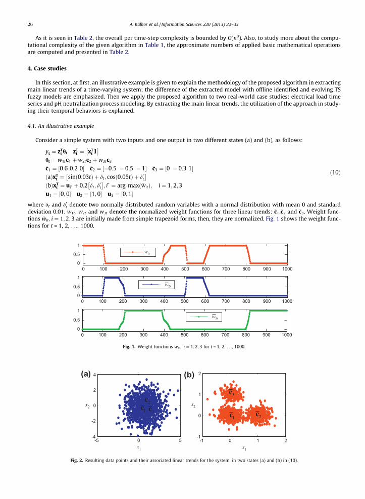
Consider a simple system with two inputs and one output in two different states (a) and (b), as follows:

yt ¼ zTt ht zT

t ¼ xTt 1

� �ht ¼ �w1t�c1 þ �w2t�c2 þ �w3t�c3

�c1 ¼ ½0:6 0:2 0� �c2 ¼ ½�0:5 � 0:5 � 1� �c3 ¼ ½0 � 0:3 1�ðaÞxT

t ¼ sinð0:03tÞ þ dt ; cosð0:05tÞ þ d0t� �

ðbÞxTt ¼ ui� þ 0:2 dt; d

0t

� �; i� ¼ argi maxð�witÞ; i ¼ 1;2;3

u1 ¼ ½0;0� u2 ¼ ½1;0� u3 ¼ ½0;1�

ð10Þ

where dt and d0t denote two normally distributed random variables with a normal distribution with mean 0 and standarddeviation 0.01. �w1t , �w2t and �w3t denote the normalized weight functions for three linear trends: �c1,�c2 and �c3. Weight func-tions �wit; i ¼ 1;2;3 are initially made from simple trapezoid forms, then, they are normalized. Fig. 1 shows the weight func-tions for t = 1, 2, . . ., 1000.

0 100 200 300 400 500 600 700 800 900 10000

0.5

1

0 100 200 300 400 500 600 700 800 900 10000

0.5

1

0 100 200 300 400 500 600 700 800 900 10000

0.5

1

tw1

tw2

tw3

Fig. 1. Weight functions �wit ; i ¼ 1;2;3 for t = 1, 2, . . ., 1000.

-5 0 5-4

-2

0

2

4

x1

x2

(a)

x1

x2

-1 0 1 2-1

0

1

2

3c

2c1c

2c

3c1c

(b)

Fig. 2. Resulting data points and their associated linear trends for the system, in two states (a) and (b) in (10).

0 100 200 300 400 500 600 700 800 900 10000

0.2

0.4(a)

0 100 200 300 400 500 600 700 800 900 1000-5

0

5

(b)

0 100 200 300 400 500 600 700 800 900 10000

5(c)

M

Fig. 3. The mean square error of real and estimated linear trends (a), the output of system and the output of its applied adaptive linear model (b), thenumber of identified clusters (c).

Table 3Mean of clusters (extracted linear trends) and the number of their members for the considered system.

Character-istics Trend State (a) State (b)

Parameters 1 c1 = [0.572 0.166 0.013] c1 = [0.572 0.186 0.025]2 c2 = [�0.506 �0.508 �0.856] c2 = [�0.511 �0.499 �0.945]3 c3 = [�0.003 �0.314 0.993] c3 = [0.005 �0.299 0.988]

Members 1 N1 = 428 N1 = 4132 N2 = 197 N2 = 1703 N3 = 374 N3 = 372

Number of identified clusters 4 5

A. Kalhor et al. / Information Sciences 220 (2013) 22–33 27

Fig. 2 shows the resulting data points and their associated linear trends in two states (a) and (b).As it is seen, in the state (a), linear trends �c1, �c2 and �c3 do not appear in certain and separated areas, whereas in state (b),

linear trends �c1, �c2 and �c3 appear in certain and separated areas. One can consider that in state (a), the system is time-varyingbut in state (b), it is not time-varying. With respect to �w1t , �w2t and �w3t , numbers of data points which belong to trends �c1, �c2

and �c3, at both states, are N1 ¼ 420, N2 ¼ 195 and N3 ¼ 385.We apply the presented algorithm in Table 1 to this system in both states for rT = 0.3 and g = 10. At first, we describe the

methodology of extracting main linear trends for state (a) through Fig. 3, but we present the final results for both statesthrough Table 3.

Fig. 3a shows the mean of square error between real and estimating linear trends of the system through the time, andFig. 3b shows the output of the system and the estimated output from the considered adaptive linear model. This figureshows obviously that the considered adaptive linear model has followed the system in state (a) for nearly all durations.The Fig. 3c shows a diagram of the number of clusters versus number of incoming data points. As it is seen, at t = 107,207 and 510 the second, third and fourth clusters are identified. Since three of them have more than 10 percent of all incom-ing data points, three main trends are extracted.

Table 3 presents more details about the extracted main linear trends in both states. It includes mean of chosen clusters (asmain linear trends) and their corresponding number of members.

It is seen from Table 3 that in both states, c1, c2 and c3 are respectively near to �c1, �c2 and �c3 and their numbers of members,N1, N2 and N3, are near to N1, N2 and N3, respectively. Later, we will introduce an index to state nearness of the extractingtrends to original ones.

To study the impact of rT on the resulting number of clusters and extracted main linear trends, we apply the algorithm tothe system in state (a) for some values of rT from 10�2 up to 1. Fig. 4 shows the resulting diagram.

As it is seen, by increasing rT, the number of clusters and extracted main linear trends is reduced. The difference betweenthe number of clusters and number of extracted main linear trends is due to some ignored clusters as explained in note 2(after Table 1).

Now, we compare our approach with TS fuzzy models about main linear trends of the system in both states. To this end,the offline and online learning algorithms of TS fuzzy model ANFIS [20], DENFIS [21], NFCRMA [25], FLEXFIS [26] and ETS [8]

10-2 10-1 100100

101

102

M: Number of total clusters

Number of extracted main trends

rT

Fig. 4. Diagram of the number of clusters and extracted main trends for some values of rT from 0.01 up to 1.

Table 4Extracting linear trends and their corresponding number of data points of TS fuzzy model identified by ANFIS.

Characteristics Trend State (a) State (b)

Parameters 1 c1 ¼ ½0:383 0:385 0:517� c1 ¼ ½0:532 0:195 0:013�2 c2 ¼ ½�0:103 � 0:815 1:466� c2 ¼ ½�0:491 � 0:490 � 0:894�3 c3 ¼ ½0:858 0:296 2:245� c3 ¼ ½�0:031 � 0:298 1:02�

Members 1 N1 ¼ 618 N1 ¼ 4192 N2 ¼ 192 N2 ¼ 1973 N3 ¼ 190 N3 ¼ 384

Table 5Extracting linear trends and their corresponding number of data points of the evolving fuzzy model identified by DENFIS.

Characteristics Trend State (a) State (b)

Parameters 1 c1 ¼ ½0:87 0:160 � 0:31� c1 ¼ ½0:401 0:508 0:282�2 c2 ¼ ½0:48 0:669 � 0:405� c2 ¼ ½0:549 � 0:507 � 0:227�3 c3 ¼ ½0:84 � 0:563 0:063� c3 ¼ ½0:973 0 � 0:218�4 c4 ¼ ½0:901 � 0:169 � 0:563� –5 c5 ¼ ½0:932 � 0:332 � 0:341� –

Members 1 N1 ¼ 122 N1 ¼ 3462 N2 ¼ 107 N2 ¼ 1533 N3 ¼ 210 N3 ¼ 2844 N4 ¼ 181 –

5 N5 ¼ 101 –

28 A. Kalhor et al. / Information Sciences 220 (2013) 22–33

are applied to the system in both states. In identified TS fuzzy models, we extract linear parameters of LLMs as linear trendsand similar to our approach, some LLMs, which have less than 10 percent members of all data points, are not considered asmain linear trends. A data point belongs to an LLM (as a member) which has maximum MF for it. Now, at first, we explain theresults achieved by applying ANFIS and DENFIS algorithms.

Table 4 presents the parameters of estimating trends and their numbers of members for the TS fuzzy model identified byANFIS algorithm for both states (a) and (b). The range of influence and the number of training epochs are chosen 0.4 and 200,respectively; all other parameters are adjusted as suggested in ANFIS algorithm.

As it is seen in Table 4, in state (a), when the system is time-varying, linear parameters of LLMs are not near to�c1; �c2 and �c3; on the contrary, in state (b), when the linear trends appear in certain areas, the extracted linear trends are nearto the system trends (�c1, �c2 and �c3Þ and their number of members are near to N1,N2 and N3.

Also, Table 5 presents the estimating trends and their number of members for evolving TS fuzzy models identified byDENFIS algorithm in states (a) and (b). All parameters are adjusted as suggested in DENFIS algorithm.

Among 19 and 20 fuzzy rules identified by DENFIS algorithm in states (a) and (b), 5 and 3 fuzzy rules, which have morethan 10 percent of all incoming data points, are considered as extracted linear trends. As it is seen in Table 5, linear param-eters of LLMs in the identified TS fuzzy model (in both states) are not near to �c1; �c2 and �c3.

Table 6Comparing Mean of Minimum Distances (MMDs) of extracting main linear trends for all applied approaches.

Approach State (a) State (b)

MMD No. of rules (clusters) MMD No. of rules (clusters)

ANFIS [20] 0.2483 3 0.0019 3NFCRMA [25] 0.3849 28 0.1201 33DENFIS [21] 0.2636 19 0.3007 20FLEXFIS [26] 0.053 8 0.0383 26ETS [8] 0.1310 6 0.0710 25Our Approach 0.0017 4 0.00054 5

0 100 200 300 400 500 600 700 800400

600

800

1000

Days

(a)

0 100 200 300 400 500 600 700 8000

1

2

Days

(b)

M

ty

ty

Fig. 5. The output of system and the output of its applied adaptive linear model (a), the number of identifying clusters (b).

A. Kalhor et al. / Information Sciences 220 (2013) 22–33 29

To state the quality of the extracting main linear trends of the system by the mentioned approaches, we define a criterion.We consider the distance index at (7); then, for each original linear trend we find an extracted linear trend with minimaldistance from the original linear trend. The criterionis defined as Mean of Minimum Distances (MMD), among all originallinear trends. Table 6 shows the computed MMD of extracting linear trends which are resulted in states (a) and (b) in(10) through the considered approaches.

Table 6 shows that our approach has significant lower MMD than other results; this shows that our proposed approachhas much better performance in extracting main linear trends. It should be noted that Table 6 does not convey any directinformation pertaining to the quality of modeling or identification. Here we just tried to compare different methods in termsof their abilities to find the original linear trends.

4.2. Electrical load time-series

Study of load consumption is one of the important tasks in power systems, which find applications ranging from powermarket to network safety. Here, an electrical load time series is considered to extract its main trends through proposed ap-proach. We used a set of data put for EUNITE network in 2001 [33]. Maximum daily values of electrical loads for 25 monthsfrom January 1997 until January 1999 are considered as a time series. We consider a process in which its output as the max-imum daily load at time t (yt) is output and the input vector is chosen to be 7 previous values (a week) of the maximum dailyload, that is,

xt ¼ ðyt�7; yt�6; . . . ; yt�1Þ ð11Þ

We apply the introduced algorithm to this process for t = 1, 2, . . ., 754, rT = 0.5 and g = 0.001. Fig. 5a shows the plots of outputof the process and output of its applied adaptive linear. As it is seen, the adaptive linear has followed it properly. Fig. 5bshows a diagram of the number of clusters versus number of days. As it is seen, the number of clusters is increased up toM = 2, thus two main linear trends are extracted for this process.

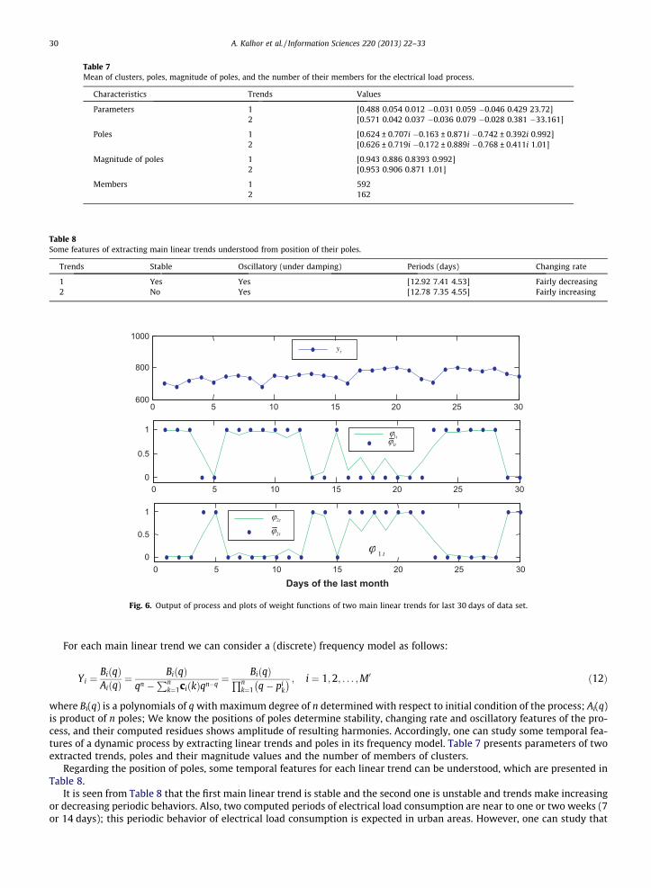
Table 7Mean of clusters, poles, magnitude of poles, and the number of their members for the electrical load process.

Characteristics Trends Values

Parameters 1 [0.488 0.054 0.012 �0.031 0.059 �0.046 0.429 23.72]2 [0.571 0.042 0.037 �0.036 0.079 �0.028 0.381 �33.161]

Poles 1 [0.624 ± 0.707i �0.163 ± 0.871i �0.742 ± 0.392i 0.992]2 [0.626 ± 0.719i �0.172 ± 0.889i �0.768 ± 0.411i 1.01]

Magnitude of poles 1 [0.943 0.886 0.8393 0.992]2 [0.953 0.906 0.871 1.01]

Members 1 5922 162

Table 8Some features of extracting main linear trends understood from position of their poles.

Trends Stable Oscillatory (under damping) Periods (days) Changing rate

1 Yes Yes [12.92 7.41 4.53] Fairly decreasing2 No Yes [12.78 7.35 4.55] Fairly increasing

0 5 10 15 20 25 30600

800

1000

0 5 10 15 20 25 300

0.5

1

0 5 10 15 20 25 300

0.5

1

Days of the last month

ty

t1ϕt1ϕ

t2ϕ

t2ϕ

t1ϕ

Fig. 6. Output of process and plots of weight functions of two main linear trends for last 30 days of data set.

30 A. Kalhor et al. / Information Sciences 220 (2013) 22–33

For each main linear trend we can consider a (discrete) frequency model as follows:

Yi ¼BiðqÞAiðqÞ

¼ BiðqÞqn �

Pnk¼1ciðkÞqn�q

¼ BiðqÞQnk¼1 q� pi

k

� � ; i ¼ 1;2; . . . ;M0 ð12Þ

where Bi(q) is a polynomials of q with maximum degree of n determined with respect to initial condition of the process; Ai(q)is product of n poles; We know the positions of poles determine stability, changing rate and oscillatory features of the pro-cess, and their computed residues shows amplitude of resulting harmonies. Accordingly, one can study some temporal fea-tures of a dynamic process by extracting linear trends and poles in its frequency model. Table 7 presents parameters of twoextracted trends, poles and their magnitude values and the number of members of clusters.

Regarding the position of poles, some temporal features for each linear trend can be understood, which are presented inTable 8.

It is seen from Table 8 that the first main linear trend is stable and the second one is unstable and trends make increasingor decreasing periodic behaviors. Also, two computed periods of electrical load consumption are near to one or two weeks (7or 14 days); this periodic behavior of electrical load consumption is expected in urban areas. However, one can study that

0 200 400 600 800 1000 1200 1400 1600 1800 20000

5

10

15

Samples

(a)

0 200 400 600 800 1000 1200 1400 1600 1800 20000

5

Samples

(b)

ty

ty

M

Fig. 7. The output of system and the output of its applied adaptive linear model (a), the number of extracted clusters (b).

Table 9Mean of clusters, poles, magnitude of poles, and the number of their members forthe considered system.

Characteristics Trend Values

Parameters 1 [�0.002 0.479 0.027 �0.202 1.045 0.846]2 [�0.113 0.185 �0.039 �0.191 0.922 4.24]

Poles 1 [0.884 0.101 ± 0.148i]2 [�0.1216 0.522 ± 0.214i]

Magnitude of poles 1 [0.844 0.179]2 [0.122 0.564]

Members 1 10602 444

Table 10Some features of transient states of main linear trends extracted from position of their corresponding poles.

Trends Transient response Time constant of damping Frequency of oscillation (HZ)

1 Under-damping 5.587 0.1552 Under-damping 8.197 0.0621

A. Kalhor et al. / Information Sciences 220 (2013) 22–33 31

what the reason of third extracted periodic behavior is. Fig. 6 shows original output of the process and plots of weight func-tions for last 30 days of data set.

The dominant trend of the process for each day is understood from Fig. 6, easily. For example, it is seen that for the inter-val between 6th day and 12th day, the first trend is dominant which provide a fairly decreasing and oscillatory change on theelectrical load consumption (from the Table 8); or for the interval between 16th day and 22nd day, the second trend is dom-inant which provide a fairly increasing and oscillatory change (from the Table 8). One can compute amplitude of resultingharmonies by considering initial conditions and solving the Eq. (12) to get more details about the temporal behavior of theprocess.

4.3. pH neutralization process

The pH neutralization process is a frequent stage in many chemical processes, which has been largely considered bychemical and material engineers. This process is performed in many applications ranged from wastewater treatments upto food industries. Here we use our proposed algorithm to extract main linear trends for simulation data of a pH neutraliza-tion process in a constant volume stirring tank [28]. The output of the process is pH of the solution in the tank and there aretwo exogenous inputs: Acid solution flow in liters and Base solution flow in liters. The volume of the tank is 1100 l; the con-centration of the acid solution (HAC) is 0.0032 Mol/l; and the concentration of the base solution (NaOH) is 0.05 Mol/l [10].The sampling time for this process is 10 s and totally 2001 data have been sampled. Since this process is inherently dynamic,we add three lags of output of process as extra inputs for the process. Now, we apply the presented algorithm in Table 1 toextract main linear trends for t = 1, 2, . . ., 1998, rT = 0.4 and g = 0.0001. Fig. 7a shows the plot of original output of process and

0 50 100 150 200 250 300 350 400 450-0.2

-0.1

0

0.1

0.2

Last 400 samples

Coefficient of first exogenous inputCoefficient of second exogenous input

Fig. 8. Plots of coefficients of exogenous inputs in the process for last 400 observed samples.

32 A. Kalhor et al. / Information Sciences 220 (2013) 22–33

the output of applied adaptive linear model. As it is seen, the adaptive linear model has followed the process, properly.Fig. 7b shows the number of clusters identified through the time. It is seen 7 clusters are identified; however, with respectto the note 2 after Table 1, just two main linear trends are extracted.

Table 9 presents parameters, poles, magnitude of poles and number of members for two extracted main linear trends.Since there are 3 lags of output as part of input, three poles for the transfer function of each linear trend are computed.

Positions of poles offer us some features about transient states of the process (Table 10).As it is seen, both trends make under-damping responses. Also, by computing time constants (as inverse of dominant

poles) and frequency of oscillation for each main linear trend, one can estimate the damping rate and the oscillation ratein transient state.

However, to study the steady state of the process, exogenous inputs and their coefficient are important. Fig. 8 shows theplots of coefficient of exogenous inputs for last 400 observed samples.

Through Fig. 8 temporal correlation between the pH level and acid or base, as exogenous inputs, can be explained for theprocess.

5. Conclusion

In this paper, to ease the studying of temporal behaviors of a nonlinear time-varying process, we introduced an approachto extract its main linear trends. For this purpose, after we constrained the process as sequential temporal linear models, afitting adaptive linear model with adaptive forgetting factor was used to follow the process and estimate its temporal lineartrends. Adaptively, the estimating trends were clustered by using a distance index and the main trends were chosen as meanof some clusters which had enough members.

The methodology and performance of the proposed approach in extraction of main linear trends were explained throughan illustrative example. It was shown that our approach –in contrast to TS fuzzy models– can extract main linear trends of asystem at both time-varying and nontime-varying states of the system. In addition, the utilization of the proposed approachin studying temporal features and transient state of processes are explained through two dynamic case studies: electricalload time series and pH neutralization process. Although the introduced approach was offered to analyze and study temporalbehaviors of a complex time-varying nonlinear process, it can be extended to be used in other applications such as predictionand control.

References

[1] J. Abonyi, R. Babuska, F. Szeifert, Modified Gath-Geva fuzzy clustering for identification of Takagi-Sugeno fuzzy models, IEEE Trans. Syst. Man, Cybern. –Part B 32 (5) (2002) 612–621.

[2] T. Alexandrov, S. Bianconcini, E.B. Dagum, P. Maass, T.S. McElroy, A review of some modern approaches to the problem of trend extraction, US CensusBureau TechReport RRS2008/03, 2008.

[3] T. Alexandrov, Software package for automatic extraction and forecast of additive components of time series in the framework of the Caterpillar-SSAapproach, PhD thesis, St.Petersburg State University, 2006 (in Russian). <http://www.pdmi.ras.ru/theo/autossa>.

[4] P. Angelov, X. Zhou, Evolving fuzzy systems from data streams in real-time, in: Proc. Int. Symp. on Evolving Fuzzy Systems, 2006, pp. 29–35.[5] P. Angelov, D. Filev, N. Kasabov (Eds.), Evolving Intelligent Systems: Methodology and Applications, John Wiley & Sons, 2010. Chapter 2, pp. 21–50.[6] P. Angelov, D. Filev, An approach to online identification of TakagiSugeno fuzzy models, IEEE Trans. Syst., Man, Cybern. B 34 (2004) 484–498.[7] P. Angelo, D. Filev, N. Kasabov, Guest editorial evolving fuzzy systems—preface to the special section, IEEE Trans. Fuzzy Syst. 16 (2008) 1390–1392.[8] P. Angelov, X. Zhou, On line learning fuzzy rule-based system structure from data streams, in: IEEE Int. Conf. on Fuzzy Systems, 2008, pp. 915–922.[9] R. Babuska, H. Verbruggen, Constructing fuzzy models by product space clustering, in: H. Hellendoorn, D. Driankov (Eds.), Fuzzy Model Identification:

Selected Approaches, Springer-Verlag, Berlin, Germany, 1997, pp. 53–90.[10] T.J. Mc Avoy, E. Hsu, S. Lowenthal, Dynamics of pH in controlled stirred tank reactor, Ind. Eng. Chem. Process Des. Develop. 11 (1972) 71–78.[11] D.S. Broomhead, G.P. King, Extracting qualitative dynamics from experimental data, Physica D: Nonlin. Phenom. 20 (1986) 217–236.[12] J.N. Choi, S.K. Oh, W. Pedrycz, Identification of fuzzy models using a successive tuning method with a variant identification ratio, Fuzzy Sets Syst. 159

(2008) 2873–2889.[13] M.R. Delgado, F.V. Zuben, F. Gomide, Hierarchical genetic fuzzy systems, Inform. Sci. 136 (2001) 29–52.

A. Kalhor et al. / Information Sciences 220 (2013) 22–33 33

[14] L.V. Fausett, Fundamentals of Neural Networks: Architectures, Algorithms and Applications, Prentice Hall, New Jersey, 1993. pp. 306.[15] G. G. Yen, P. Meesad, An effective neuro-fuzzy paradigm for machinery condition health monitoring, in: Proc. IEEE Int. Joint Conf. IJCNN’99,

Washington, DC, 1999, pp. 1567–1572.[16] S. Haykin, Adaptive Filter Theory, Prentice Hall, New Jersey, 2002.[17] M. Hell, R. Ballini, P. Costa Jr., F. Gomide, Training neurofuzzy networkswith participatory learning, Proc. 5th Conf. of the EUSFLAT 2 (2007) 231–236.[18] F. Hoffmann, O. Nelles, Genetic programming for model selection of TSK-fuzzy systems original research article, Inform. Sci. 136 (2001) 7–28.[19] R.A. Jacobs, Increased rates of convergence through learning rate adaptation, Neur. Netw. 1 (1998) 295–308.[20] J.S.R. Jang, ANFIS: adaptive-network-based fuzzy inference system, IEEE Trans. Syst. Man, Cybern. 23 (3) (1993) 665–685.[21] N. Kasabov, DENFIS: dynamic evolving neural-fuzzy inference system and its application for time series prediction, IEEE Trans. Fuzzy Syst. (2002) 144–

154.[22] A. Kalhor, B.N. Araabi, C. Lucas, A new split and merge algorithm for structure identification in Takagi-Sugeno fuzzy model, in: Proc. 7th IEEE Int. Conf.

on Intelligent Systems Design and Applications, 2007, pp. 258–261.[23] A. Kalhor, B.N. Araabi, C. Lucas, Online identification of a neurofuzzy model through indirect fuzzy clustering of data space, in: Proc. 18th IEEE Int. Conf.

on Fuzzy Systems, 2009, pp. 356–359.[24] A. Kalhor, B.N. Araabi, C. Lucas, An online predictor model as adaptive habitually linear and transiently nonlinear model, Evolv. Syst. 1 (2010) 29–41.[25] C. Li, J. Zhou, X. Xiang, Q. Li, X. An, T–S fuzzy model identification based on a novel fuzzy c-regression model clustering algorithm, Eng. Appl. Artif. Intell.

22 (2009) 646–653.[26] E.D. Lughofer, FLEXFIS: a robust incremental learning approach for evolving Takagi–Sugeno fuzzy models, IEEE Trans. Fuzzy Syst. 16 (2008) 1393–

1410.[27] C.E.V. Leser, A simple method of trend construction, J. Roy. Stat. Soc.: Ser. B (Methodol.) 23 (1961) 91–107.[28] B.L.R. De Moor (Ed.), DaISy: Database for the Identification of Systems, Department of Electrical Engineering, ESAT/SISTA, K.U.Leuven, Belgium, <http://

homes.esat.kuleuven.be/ � smc/daisy/> (visited on 10.10.10).[29] O. Nelles, Nonlinear System Identification, New York: Springer, Section 13.3.1, 2001, pp. 365–372.[30] B. Rezaee, M.H. Fazel Zarandi, Data-driven fuzzy modeling for Takagi–Sugeno–Kang fuzzy system, Inform. Sci. 180 (2010) 241–255.[31] A. Schönhage, A.F.W. Grotefeld, E. Vetter, Fast algorithms—a multitape turing machine implementation, BI Wissenschafts-Verlag, Mannheim, 1994.[32] T. Takagi, M. Sugeno, Fuzzy identification of systems and its applications to modeling and control, IEEE Trans. Syst. Man, Cybern. 15 (1) (1985) 116–

132.[33] The homepage of World-wide competition within the EUNITE network: <http://neuron-ai.tuke.sk/competition/>. (visited on 10.10.10).[34] D. Wang, C. Quek, G.S. Ng, MS-TSKfnn: novel Takagi-Sugeno-Kang fuzzy neural network using ART like clustering, Proc. IEEE Int. Joint Conf. Neur. Netw.

3 (2004) 2361–2366.[35] L. Wang, J. Mendel, Fuzzy basis functions, universal approximation and orthogonal least-squares learning, IEEE Trans. Neur. Netw. 3 (1992) 807–814.[36] L. Wang, J. Yen, Extracting fuzzy rules for system modeling using a hybrid of genetic algorithm and Kalman filter, Fuzzy Sets Syst. 101 (1999) 353–362.[37] M. Weir, A method for self-determination of adaptive learning rates in back propagation, Neur. Netw. 4 (1991) 371–379.[38] R. Yager, D. Filev, Essentials of Fuzzy Modeling and Control, John Wiley, NY, 1994.[39] R. Yager, D. Filev, Generation of fuzzy rules by mountain clustering, Machine Intelligence Institute, Iona College, New Rochelle, NY 10801, Tech. Rep.

MII-1318R, 1994.