Embed Size (px)
Citation preview
Online Computation of Fastest Path in Time-DependentSpatial Networks�
Ugur Demiryurek1, Farnoush Banaei-Kashani1, Cyrus Shahabi1,and Anand Ranganathan2
1 University of Southern California- Department of Computer ScienceLos Angeles, CA USA
{demiryur,banaeika,shahabi}@usc.edu2 IBM T.J. Watson Research Center
Hawthorne, NY [email protected]
Abstract. The problem of point-to-point fastest path computation in static spa-tial networks is extensively studied with many precomputation techniques pro-posed to speed-up the computation. Most of the existing approaches make thesimplifying assumption that travel-times of the network edges are constant. How-ever, with real-world spatial networks the edge travel-times are time-dependent,where the arrival-time to an edge determines the actual travel-time on the edge. Inthis paper, we study the online computation of fastest path in time-dependent spa-tial networks and present a technique which speeds-up the path computation. Weshow that our fastest path computation based on a bidirectional time-dependentA* search significantly improves the computation time and storage complexity.With extensive experiments using real data-sets (including a variety of large spa-tial networks with real traffic data) we demonstrate the efficacy of our proposedtechniques for online fastest path computation.
1 Introduction
With the ever-growing popularity of online map applications and their wide deploymentin mobile devices and car-navigation systems, an increasing number of users search forpoint-to-point fastest paths and the corresponding travel-times. On static road networkswhere edge costs are constant, this problem has been extensively studied and manyefficient speed-up techniques have been developed to compute the fastest path in a mat-ter of milliseconds (e.g., [27,31,28,29]). The static fastest path approaches make thesimplifying assumption that the travel-time for each edge of the road network is con-stant (e.g., proportional to the length of the edge). However, in real-world the actualtravel-time on a road segment heavily depends on the traffic congestion and, therefore,is a function of time i.e., time-dependent. For example, Figure 1 shows the variation
� This research has been funded in part by NSF grants IIS-0238560 (PECASE), IIS-0534761,IIS-0742811 and CNS-0831505 (CyberTrust), and in part from CENS andMETRANS Transportation Center, under grants from USDOT and Caltrans.Any opinions,findings, and conclusions or recommendations expressed in this material are those of the au-thor(s) and do not necessarily reflect the views of the National Science Foundation.
D. Pfoser et al. (Eds.): SSTD 2011, LNCS 6849, pp. 92–111, 2011.c© Springer-Verlag Berlin Heidelberg 2011
Online Computation of Fastest Path in Time-Dependent Spatial Networks 93
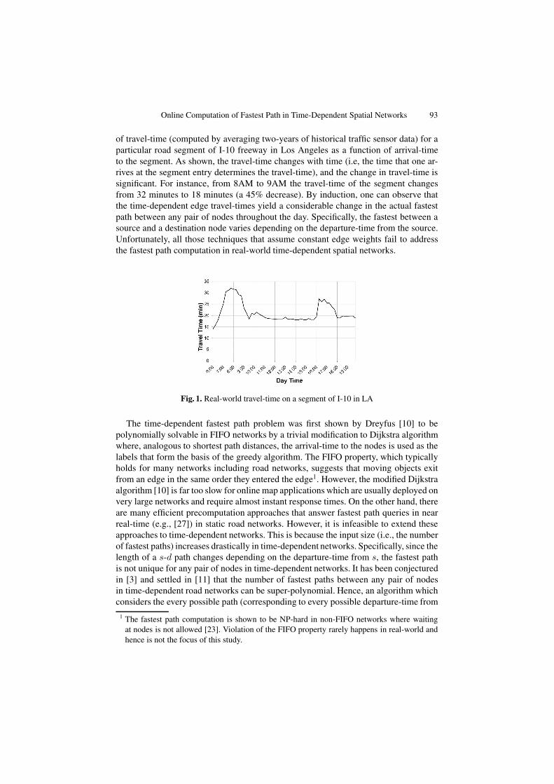
of travel-time (computed by averaging two-years of historical traffic sensor data) for aparticular road segment of I-10 freeway in Los Angeles as a function of arrival-timeto the segment. As shown, the travel-time changes with time (i.e, the time that one ar-rives at the segment entry determines the travel-time), and the change in travel-time issignificant. For instance, from 8AM to 9AM the travel-time of the segment changesfrom 32 minutes to 18 minutes (a 45% decrease). By induction, one can observe thatthe time-dependent edge travel-times yield a considerable change in the actual fastestpath between any pair of nodes throughout the day. Specifically, the fastest between asource and a destination node varies depending on the departure-time from the source.Unfortunately, all those techniques that assume constant edge weights fail to addressthe fastest path computation in real-world time-dependent spatial networks.
Fig. 1. Real-world travel-time on a segment of I-10 in LA
The time-dependent fastest path problem was first shown by Dreyfus [10] to bepolynomially solvable in FIFO networks by a trivial modification to Dijkstra algorithmwhere, analogous to shortest path distances, the arrival-time to the nodes is used as thelabels that form the basis of the greedy algorithm. The FIFO property, which typicallyholds for many networks including road networks, suggests that moving objects exitfrom an edge in the same order they entered the edge1. However, the modified Dijkstraalgorithm [10] is far too slow for online map applications which are usually deployed onvery large networks and require almost instant response times. On the other hand, thereare many efficient precomputation approaches that answer fastest path queries in nearreal-time (e.g., [27]) in static road networks. However, it is infeasible to extend theseapproaches to time-dependent networks. This is because the input size (i.e., the numberof fastest paths) increases drastically in time-dependent networks. Specifically, since thelength of a s-d path changes depending on the departure-time from s, the fastest pathis not unique for any pair of nodes in time-dependent networks. It has been conjecturedin [3] and settled in [11] that the number of fastest paths between any pair of nodesin time-dependent road networks can be super-polynomial. Hence, an algorithm whichconsiders the every possible path (corresponding to every possible departure-time from
1 The fastest path computation is shown to be NP-hard in non-FIFO networks where waitingat nodes is not allowed [23]. Violation of the FIFO property rarely happens in real-world andhence is not the focus of this study.
94 U. Demiryurek et al.
the source) for any pair of nodes in large time-dependent networks would suffer fromexponential time and prohibitively large storage requirements. For example, the time-dependent extension of Contraction Hierarchies (CH) [1] and SHARC [5] speed-uptechniques (which are proved to be very efficient for static networks) suffer from theimpractical precomputation times and intolerable storage complexity (see Section 3).
In this study, we propose a bidirectional time-dependent fastest path algorithm (B-TDFP) based on A* search [17]. There are two main challenges to employ bidirectionalA* search in time-dependent networks. First, finding an admissible heuristic function(i.e., lower-bound distance) between an intermediate vi node and the destination d ischallenging as the distance between vi and d changes based on the departure-time fromvi. Second, it is not possible to implement a backward search without knowing thearrival-time at the destination. We address the former challenge by partitioning the roadnetwork to non-overlapping partitions (an off-line operation) and precompute the intra(node-to-border) and inter (border-to-border) partition distance labels with respect toLower-bound Graph G which is generated by substituting the edge travel-times in Gwith minimum possible travel-times. We use the combination of intra and inter distancelabels as a heuristic function in the online computation. To address the latter challenge,we run the backward search on the lower-bound graph (G) which enables us to filter-inthe set of the nodes that needs to be explored by the forward search.
The remainder of this paper is organized as follows. In Section 2, we explain theimportance of time-dependency for accurate and useful path planning. In Section 3, wereview the related work on time-dependent fastest path algorithms. In Section 4, weformally define the time-dependent fastest path problem in spatial networks. In Sec-tion 5, we establish the theoretical foundation of our proposed bidirectional algorithmand explain our approach. In Section 6, we present the results of our experiments forboth approaches with a variety of spatial networks with real-world time-dependent edgeweights. Finally, in Section 7, we conclude and discuss our future work.
2 Towards Time-Dependent Path Planning
In this section, we explain the difference between fastest computation in time-dependentand static spatial networks. We also discuss the importance and the feasibility of time-dependent route planning.
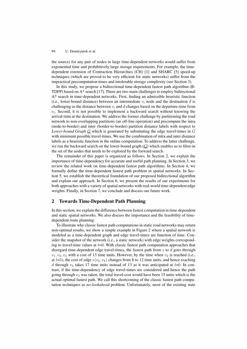
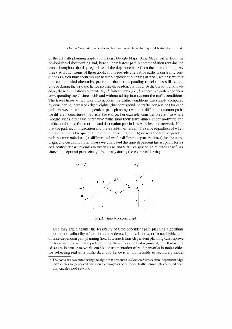
To illustrate why classic fastest path computations in static road networks may returnnon-optimal results, we show a simple example in Figure 2 where a spatial network ismodeled as a time-dependent graph and edge travel-times are function of time. Con-sider the snapshot of the network (i.e., a static network) with edge weights correspond-ing to travel-time values at t=0. With classic fastest path computation approaches thatdisregard time-dependent edge travel-times, the fastest path from s to d goes throughv1, v2, v4 with a cost of 13 time units. However, by the time when v2 is reached (i.e.,at t=5), the cost of edge e(v2, v4) changes from 8 to 12 time units, and hence reachingd through v2 takes 17 time units instead of 13 as it was anticipated at t=0. In con-trast, if the time-dependency of edge travel-times are considered and hence the pathgoing through v3 was taken, the total travel-cost would have been 15 units which is theactual optimal fastest path. We call this shortcoming of the classic fastest path compu-tation techniques as no-lookahead problem. Unfortunately, most of the existing state
Online Computation of Fastest Path in Time-Dependent Spatial Networks 95
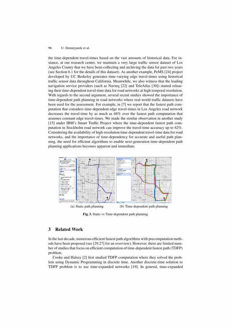
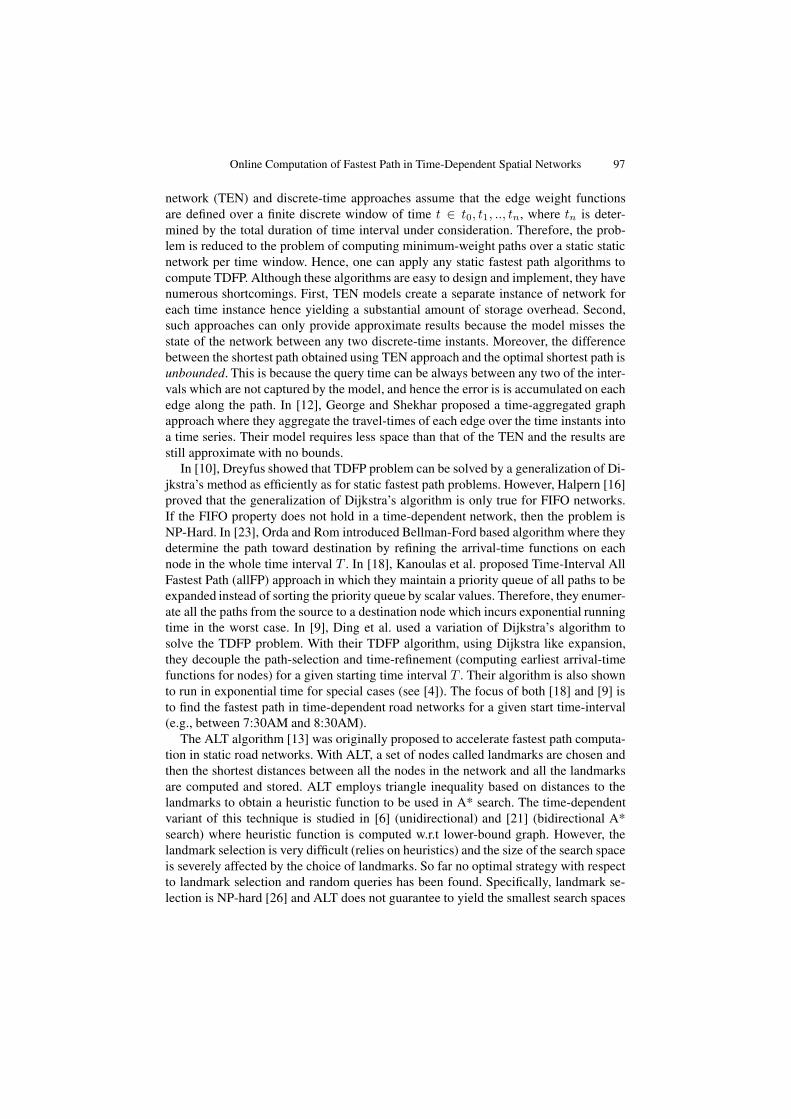
of the art path planning applications (e.g., Google Maps, Bing Maps) suffer from theno-lookahead shortcoming and, hence, their fastest path recommendation remains thesame throughout the day regardless of the departure-time from the source (i.e., querytime). Although some of these applications provide alternative paths under traffic con-ditions (which may seem similar to time-dependent planning at first), we observe thatthe recommended alternative paths and their corresponding travel-times still remainunique during the day, and hence no time-dependent planning. To the best of our knowl-edge, these applications compute top-k fastest paths (i.e., k alternative paths) and theircorresponding travel-times with and without taking into account the traffic conditions.The travel-times which take into account the traffic conditions are simply computedby considering increased edge weights (that corresponds to traffic congestion) for eachpath. However, our time-dependent path planning results in different optimum pathsfor different departure-times from the source. For example, consider Figure 3(a) whereGoogle Maps offer two alternative paths (and their travel-times under no-traffic andtraffic conditions) for an origin and destination pair in Los Angeles road network. Notethat the path recommendation and the travel-times remain the same regardless of whenthe user submits the query. On the other hand, Figure 3(b) depicts the time-dependentpath recommendations (in different colors for different departure times) for the sameorigin and destination pair where we computed the time-dependent fastest paths for 38consecutive departure-times between 8AM and 5:30PM, spaced 15 minutes apart2. Asshown, the optimal paths change frequently during the course of the day.
Fig. 2. Time-dependent graph
One may argue against the feasibility of time-dependent path planning algorithmsdue to a) unavailability of the time-dependent edge travel-times, or b) negligible gainof time-dependent path planning (i.e., how much time-dependent planning can improvethe travel-time) over static path planning. To address the first argument, note that recentadvances in sensor networks enabled instrumentation of road networks in major citiesfor collecting real-time traffic data, and hence it is now feasible to accurately model
2 The paths are computed using the algorithm presented in Section 5 where time-dependent edgetravel-times are generated based on the two-years of historical traffic sensor data collected fromLos Angeles road network.
96 U. Demiryurek et al.
the time-dependent travel-times based on the vast amounts of historical data. For in-stance, at our research center, we maintain a very large traffic sensor dataset of LosAngeles County that we have been collecting and archiving the data for past two years(see Section 6.1 for the details of this dataset). As another example, PeMS [24] projectdeveloped by UC Berkeley generates time-varying edge travel-times using historicaltraffic sensor data throughout California. Meanwhile, we also witness that the leadingnavigation service providers (such as Navteq [22] and TeleAtlas [30]) started releas-ing their time-dependent travel-time data for road networks at high temporal resolution.With regards to the second argument, several recent studies showed the importance oftime-dependent path planning in road networks where real-world traffic datasets havebeen used for the assessment. For example, in [7] we report that the fastest path com-putation that considers time-dependent edge travel-times in Los Angeles road networkdecreases the travel-time by as much as 68% over the fastest path computation thatassumes constant edge travel-times. We made the similar observation in another study[15] under IBM’s Smart Traffic Project where the time-dependent fastest path com-putation in Stockholm road network can improve the travel-time accuracy up to 62%.Considering the availability of high-resolution time-dependent travel-time data for roadnetworks, and the importance of time-dependency for accurate and useful path plan-ning, the need for efficient algorithms to enable next-generation time-dependent pathplanning applications becomes apparent and immediate.
(a) Static path planning (b) Time-dependent path planning
Fig. 3. Static vs Time-dependent path planning
3 Related Work
In the last decade, numerous efficient fastest path algorithms with precomputation meth-ods have been proposed (see [29,27] for an overview). However, there are limited num-ber of studies that focus on efficient computation of time-dependent fastest path (TDFP)problem.
Cooke and Halsey [2] first studied TDFP computation where they solved the prob-lem using Dynamic Programming in discrete time. Another discrete-time solution toTDFP problem is to use time-expanded networks [19]. In general, time-expanded
Online Computation of Fastest Path in Time-Dependent Spatial Networks 97
network (TEN) and discrete-time approaches assume that the edge weight functionsare defined over a finite discrete window of time t ∈ t0, t1, .., tn, where tn is deter-mined by the total duration of time interval under consideration. Therefore, the prob-lem is reduced to the problem of computing minimum-weight paths over a static staticnetwork per time window. Hence, one can apply any static fastest path algorithms tocompute TDFP. Although these algorithms are easy to design and implement, they havenumerous shortcomings. First, TEN models create a separate instance of network foreach time instance hence yielding a substantial amount of storage overhead. Second,such approaches can only provide approximate results because the model misses thestate of the network between any two discrete-time instants. Moreover, the differencebetween the shortest path obtained using TEN approach and the optimal shortest path isunbounded. This is because the query time can be always between any two of the inter-vals which are not captured by the model, and hence the error is is accumulated on eachedge along the path. In [12], George and Shekhar proposed a time-aggregated graphapproach where they aggregate the travel-times of each edge over the time instants intoa time series. Their model requires less space than that of the TEN and the results arestill approximate with no bounds.
In [10], Dreyfus showed that TDFP problem can be solved by a generalization of Di-jkstra’s method as efficiently as for static fastest path problems. However, Halpern [16]proved that the generalization of Dijkstra’s algorithm is only true for FIFO networks.If the FIFO property does not hold in a time-dependent network, then the problem isNP-Hard. In [23], Orda and Rom introduced Bellman-Ford based algorithm where theydetermine the path toward destination by refining the arrival-time functions on eachnode in the whole time interval T . In [18], Kanoulas et al. proposed Time-Interval AllFastest Path (allFP) approach in which they maintain a priority queue of all paths to beexpanded instead of sorting the priority queue by scalar values. Therefore, they enumer-ate all the paths from the source to a destination node which incurs exponential runningtime in the worst case. In [9], Ding et al. used a variation of Dijkstra’s algorithm tosolve the TDFP problem. With their TDFP algorithm, using Dijkstra like expansion,they decouple the path-selection and time-refinement (computing earliest arrival-timefunctions for nodes) for a given starting time interval T . Their algorithm is also shownto run in exponential time for special cases (see [4]). The focus of both [18] and [9] isto find the fastest path in time-dependent road networks for a given start time-interval(e.g., between 7:30AM and 8:30AM).
The ALT algorithm [13] was originally proposed to accelerate fastest path computa-tion in static road networks. With ALT, a set of nodes called landmarks are chosen andthen the shortest distances between all the nodes in the network and all the landmarksare computed and stored. ALT employs triangle inequality based on distances to thelandmarks to obtain a heuristic function to be used in A* search. The time-dependentvariant of this technique is studied in [6] (unidirectional) and [21] (bidirectional A*search) where heuristic function is computed w.r.t lower-bound graph. However, thelandmark selection is very difficult (relies on heuristics) and the size of the search spaceis severely affected by the choice of landmarks. So far no optimal strategy with respectto landmark selection and random queries has been found. Specifically, landmark se-lection is NP-hard [26] and ALT does not guarantee to yield the smallest search spaces
98 U. Demiryurek et al.
with respect to fastest path computations where source and destination nodes are cho-sen at random. Our experiments with real-world time-dependent travel-times show thatour approach consumes much less storage as compared to ALT based approaches andyields faster response times (see Section 6). In two different studies, The ContractionHierarchies (CH) and SHARC methods (also developed for static networks) were aug-mented to time-dependent road networks in [1] and [5], respectively. The main idea ofthese techniques is to remove unimportant nodes from the graph without changing thefastest path distances between the remaining (more important) nodes. However, unlikethe static networks, the importance of a node can change throughout the time underconsideration in time-dependent networks, hence the importance of the nodes are timevarying. Considering the super-polynomial input size (as discussed in Section 1), andhence the super-polynomial number of important nodes with time-dependent networks,the main shortcomings of these approaches are impractical preprocessing times and ex-tensive space consumption. For example, the precomputation time for SHARC in time-dependent road networks takes more than 11 hours for relatively small road networks(e.g. LA with 304,162 nodes) [5]. Moreover, due to the significant use of arc flags [5],SHARC does not work in a dynamic scenario: whenever an edge cost function changes,arc flags should be recomputed, even though the graph partition need not be updated.While CH also suffers from slow preprocessing times, the space consumption for CHis at least 1000 bytes per node for less varied edge-weights where the storage cost in-creases with real-world time-dependent edge weights. Therefore, it may not be feasibleto apply SHARC and CH to continental size road networks which can consist of morethan 45 million road segments (e.g., North America road network) with possibly largevaried edge-weights.
4 Problem Definition
There are various criteria to define the cost of a path in road networks. In our studywe define the cost of a path as its travel-time. We model the road network as a time-dependent weighted graph as shown in Figure 2 where time-dependent travel-times areprovided as a function of time which captures the typical congestion pattern for eachsegment of the road network. We use piecewise linear functions to represent the time-dependent travel-times in the network.
Definition 1. Time-dependent Graph. A Time-dependent Graph is defined as G(V, E,T ) where V = {vi} is a set of nodes and E ⊆ V × V is a set of edges representingthe network segments each connecting two nodes. For every edge e(vi, vj) ∈ E, andvi �= vj , there is a cost function cvi,vj (t), where t is the time variable in time domain T .An edge cost function cvi,vj (t) specifies the travel-time from vi to vj starting at time t.
Definition 2. Time-dependent Travel Cost. Let {s = v1, v2, ..., vk = d} denotes apath which contains a sequence of nodes where e(vi, vi+1) ∈ E and i = 1, ..., k − 1.Given a G(V, E, T ), a path (s � d) from source s to destination d, and a departure-time at the source ts, the time-dependent travel cost TT (s� d, ts) is the time it takesto travel the path. Since the travel-time of an edge varies depending on the arrival-timeto that edge, the travel-time of a path is computed as follows:

Online Computation of Fastest Path in Time-Dependent Spatial Networks 99
TT (s� d, ts) =k−1∑
i=1
cvi,vi+1(ti) where t1 = ts, ti+1 = ti + c(vi,vi+1)(ti), i = 1, .., k.
Definition 3. Lower-bound Graph. Given a G(V, E, T ), the corresponding Lower-bound Graph G(V, E) is a graph with the same topology (i.e, nodes and edges) asgraph G, where the weight of each edge cvi,vj is fixed (not time-dependent) and is equalto the minimum possible weight cmin
vi,vjwhere ∀ e(vi, vj) ∈ E, t ∈ T cmin
vi,vj≤ cvi,vj (t).
Definition 4. Lower-bound Travel Cost. The lower-bound travel-time LTT (s � d)of a path is less than the actual travel-time along that path and computed w.r.t G(V, E)as
LTT (s� d) =k−1∑
i=1
cminvi,vi+1
, i = 1, .., k.
It is important to note that for each source and destination pair (s, d), LTT (s � d)is time-independent constant value and hence t is not included in its definition. Giventhe definitions of TT and LTT , the following property always holds for any path inG(V, E, T ): LTT (s � d) ≤ TT (s � d, ts) where ts is an arbitrary departure-timefrom s. We will use this property in subsequent sections to establish some properties ofour proposed solution.
Definition 5. Time-dependent Fastest Path (TDFP). Given a G(V, E, T ), s, d, andts, the time-dependent fastest path TDFP (s, d, ts) is a path with the minimum travel-time among all paths from s to d for starting time ts.
In the rest of this paper, we assume that G(V, E, T ) satisfies the First-In-First-Out(FIFO) property. We also assume that moving objects do not wait at any node. In mostreal-world applications, waiting at a node is not realistic as it means that the movingobject must interrupt its travel by getting out of a road (e.g., exit freeway), and findinga place to park and wait.
5 Time-Dependent Fastest Path Computation
In this section, we explain our bidirectional time-dependent fastest path approach thatwe generalize bidirectional A* algorithm proposed for static spatial networks [25] totime-dependent road networks. Our proposed solution involves two phases. At the pre-computation phase, we partition the road network into non-overlapping partitions andprecompute lower-bound distance labels within and across the partitions with respectto G(V, E). Successively, at the online phase, we use the precomputed distance labelsas a heuristic function in our bidirectional time-dependent A* search that performs si-multaneous searches from source and destination. Below we elaborate on both phases.
5.1 Precomputation Phase
The precomputation phase of our proposed algorithm includes two main steps in whichwe partition the road network into non-overlapping partitions and precompute lower-bound border-to-border, node-to-border, and border-to-node distance labels.
100 U. Demiryurek et al.
5.1.1 Road Network PartitioningReal-world road networks are built on a well-defined hierarchy. For example, in UnitedStates, highways connect large regions such as states, interstate roads connect citieswithin a state, and multi-lane roads connect locations within a city. Almost all of theroad network data providers (e.g., Navteq [22]) include road hierarchy information intheir datasets. In this paper, we partition the graph to non-overlapping partitions byexploiting the predefined edge class information in road networks. Specifically, we firstuse higher level roads (e.g., interstate) to divide the road network into large regions.Then, we subdivide each large region using the next level roads and so on. We adoptthis technique from [14] and note that our proposed algorithm is independent of thepartitioning method, i.e., it yields correct results with all non-overlapping partitioningmethods.
With our approach, we assume that the class of each edge class(e) is predefined andwe denote the class of a node class(v) by the lowest class number of any incomingor outgoing edge to/from v. For instance, a node at the intersection of two freewaysegments and an arterial road (i.e., the entry node to the freeway) is labeled with classof the freeway rather than the class of the arterial road. The input to our hierarchicalpartitioning method is the road network and the level of partitioning l. For example,if we like to partition a particular road network based on the interstates, freeways, andarterial roads in sequence, we set l = 2 where interstate edges represent the class 0.The road network partitions can be conceptually visualized as the areas after removalthe nodes with class(v) ≤ l from G(E, V ).
Definition 6. Given a graph G(V, E), the partition of G(V, E) is a set of subgraphs{S1, S2, ..., Sk} where Si = (Vi, Ei) includes node set Vi where Vi ∩ Vj = ∅ and∪k
i=1Vi = V , i �= j.
Given a G(E, V ) and level of partitioning l, we first assign to each node an empty setof partitions. Then, we choose a node vi that is connected to edges other than the onesused for partitioning (i.e., a node with class(vi) > l) and add partition number (e.g.,S1) to vi’s partition set. For instance, continuing with our example above, a node vi withclass(vi) > 2 represent a particular node that belongs a less important road segmentthan an arterial road. Subsequently, we expand a shortest path tree from vi to all it’sneighbor nodes reachable through the edges of the classes greater than l, and add S1 totheir partition sets. Intuitively, we expand from vi until we reach the roads that are usedfor partitioning. At this point we determine all the nodes that belong to S1. Then, weselect another node vj with an empty partition set by adding the next partition number(e.g., S2) to vj’s partition set and repeat the process. We terminate the process whenall nodes are assigned to at least one partition. With this method we can easily find theborder nodes for each partition, i.e., those nodes which include multiple partitions intheir partition sets. Specifically, a node v, with class(v) ≤ l belongs to all partitionssuch that there is an edge e (with class(e) > l) connecting v to v′ where v′ ∈ Si andi = 1, ..., k, is the border node of the partitions that it connects to. Note that l is a tuningparameter in our partitioning method. Hence, one can arrange the size of the partitionsby increasing or decreasing l.
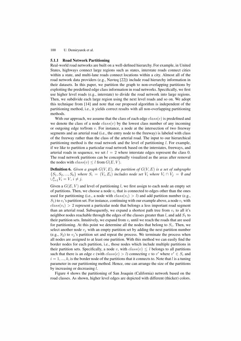
Figure 4 shows the partitioning of San Joaquin (California) network based on theroad classes. As shown, higher level edges are depicted with different (thicker) colors.
Online Computation of Fastest Path in Time-Dependent Spatial Networks 101
Fig. 4. Road network partitioning
Each partition is numbered starting from the north-west corner of the road network. Theborder nodes between partitions S1 and S4 are shown in the circled area. We remarkthat the number of border nodes (which can be potentially large depending on the den-sity of the network) in the actual partitions have a negligible influence on the storagecomplexity. We explain the effect of the border nodes on the storage cost in the nextsection.
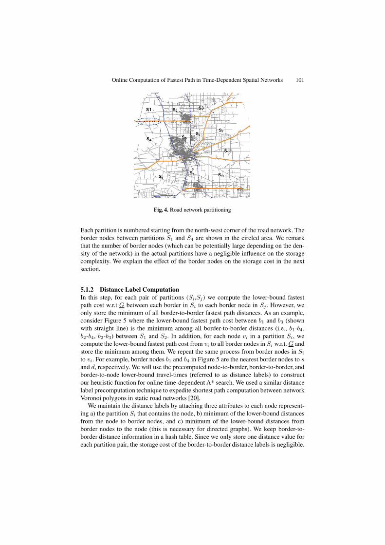
5.1.2 Distance Label ComputationIn this step, for each pair of partitions (Si,Sj) we compute the lower-bound fastestpath cost w.r.t G between each border in Si to each border node in Sj . However, weonly store the minimum of all border-to-border fastest path distances. As an example,consider Figure 5 where the lower-bound fastest path cost between b1 and b3 (shownwith straight line) is the minimum among all border-to-border distances (i.e., b1-b4,b2-b4, b2-b3) between S1 and S2. In addition, for each node vi in a partition Si, wecompute the lower-bound fastest path cost from vi to all border nodes in Si w.r.t. G andstore the minimum among them. We repeat the same process from border nodes in Si
to vi. For example, border nodes b1 and b4 in Figure 5 are the nearest border nodes to sand d, respectively. We will use the precomputed node-to-border, border-to-border, andborder-to-node lower-bound travel-times (referred to as distance labels) to constructour heuristic function for online time-dependent A* search. We used a similar distancelabel precomputation technique to expedite shortest path computation between networkVoronoi polygons in static road networks [20].
We maintain the distance labels by attaching three attributes to each node represent-ing a) the partition Si that contains the node, b) minimum of the lower-bound distancesfrom the node to border nodes, and c) minimum of the lower-bound distances fromborder nodes to the node (this is necessary for directed graphs). We keep border-to-border distance information in a hash table. Since we only store one distance value foreach partition pair, the storage cost of the border-to-border distance labels is negligible.
102 U. Demiryurek et al.
Fig. 5. Lower-bound distance computation
Another benefit of our proposed lower-bound computation is that the lower-boundsneed to be updated when it is necessary. Specifically, we update the intra and inter dis-tance labels only when the minimum travel-time of an edge changes, otherwise, thetravel-time updates are discarded. Note that intra distance label computation is local,i.e., we only update the intra distance labels for the partitions in which the minimumtravel-time of an edge changes.
5.2 Online B-TDFP Computation
As showed in [10], the time-dependent fastest path problem (in FIFO networks) canbe solved by modifying Dijkstra algorithm. We refer to modified Dijkstra algorithm astime-dependent Dijkstra (TD-Dijkstra). TD-Dijkstra visits all network nodes reachablefrom s in every direction until destination node d is reached. On the other hand, a time-dependent A* algorithm can significantly reduce the number of nodes that have to betraversed in TD-Dijkstra algorithm by employing a heuristic function h(v) that directsthe search towards destination. To guarantee optimal results, h(v) must be admissibleand consistent (a.k.a, monotonic). The admissibility implies that h(v) must be less thanor equal to the actual distance between v and d. With static road networks where thelength of an edge is constant, Euclidian distance between v and d is used as h(v).However, this simple heuristic function cannot be directly applied to time-dependentroad networks, because, the optimal travel-time between v and d changes based on thedeparture-time tv from v. Therefore, in time-dependent road networks, we need to usean estimator that never overestimates the travel-time between v and d for any possibletv. One simple lower-bound estimator is deuc(v, d)/max(speed), i.e., the Euclideandistance between v and d divided by the maximum speed among the edges in the entirenetwork. Although this estimator is guaranteed to be a lower-bound, it is a very loosebound, and hence yields insignificant pruning.
With our approach, we obtain a much tighter bound by utilizing the precomputeddistance labels. Assuming that an on-line time-dependent fastest path query requests apath from source s in partition Si to destination d in partition Sj , the fastest path mustpass through from one border node bi in Si and another border node bj in Sj . We knowthat the time-dependent fastest path distance passing from bi and bj is greater than orequal to the precomputed lower-bound border-to-border (e.g., LTT (bl, bt)) distance forSi and Sj pair. We also know that a time-dependent fastest path distance from s to bi
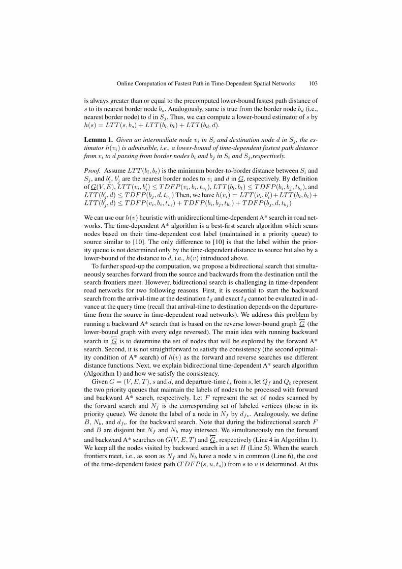
Online Computation of Fastest Path in Time-Dependent Spatial Networks 103
is always greater than or equal to the precomputed lower-bound fastest path distance ofs to its nearest border node bs. Analogously, same is true from the border node bd (i.e.,nearest border node) to d in Sj . Thus, we can compute a lower-bound estimator of s byh(s) = LTT (s, bs) + LTT (bl, bt) + LTT (bd, d).
Lemma 1. Given an intermediate node vi in Si and destination node d in Sj , the es-timator h(vi) is admissible, i.e., a lower-bound of time-dependent fastest path distancefrom vi to d passing from border nodes bi and bj in Si and Sj ,respectively.
Proof. Assume LTT (bl, bt) is the minimum border-to-border distance between Si andSj , and b′i, b′j are the nearest border nodes to vi and d in G, respectively. By definitionof G(V, E), LTT (vi, b
′i) ≤ TDFP (vi, bi, tvi), LTT (bl, bt) ≤ TDFP (bi, bj, tbi), and
LTT (b′j, d) ≤ TDFP (bj, d, tbj ) Then, we have h(vi) = LTT (vi, b′i)+LTT (bl, bt)+
LTT (b′j, d) ≤ TDFP (vi, bi, tvi) + TDFP (bi, bj , tbi) + TDFP (bj, d, tbj )
We can use our h(v) heuristic with unidirectional time-dependent A* search in road net-works. The time-dependent A* algorithm is a best-first search algorithm which scansnodes based on their time-dependent cost label (maintained in a priority queue) tosource similar to [10]. The only difference to [10] is that the label within the prior-ity queue is not determined only by the time-dependent distance to source but also by alower-bound of the distance to d, i.e., h(v) introduced above.
To further speed-up the computation, we propose a bidirectional search that simulta-neously searches forward from the source and backwards from the destination until thesearch frontiers meet. However, bidirectional search is challenging in time-dependentroad networks for two following reasons. First, it is essential to start the backwardsearch from the arrival-time at the destination td and exact td cannot be evaluated in ad-vance at the query time (recall that arrival-time to destination depends on the departure-time from the source in time-dependent road networks). We address this problem byrunning a backward A* search that is based on the reverse lower-bound graph
←−G (the
lower-bound graph with every edge reversed). The main idea with running backwardsearch in
←−G is to determine the set of nodes that will be explored by the forward A*
search. Second, it is not straightforward to satisfy the consistency (the second optimal-ity condition of A* search) of h(v) as the forward and reverse searches use differentdistance functions. Next, we explain bidirectional time-dependent A* search algorithm(Algorithm 1) and how we satisfy the consistency.
Given G = (V, E, T ), s and d, and departure-time ts from s, let Qf and Qb representthe two priority queues that maintain the labels of nodes to be processed with forwardand backward A* search, respectively. Let F represent the set of nodes scanned bythe forward search and Nf is the corresponding set of labeled vertices (those in itspriority queue). We denote the label of a node in Nf by dfv. Analogously, we defineB, Nb, and dfv for the backward search. Note that during the bidirectional search Fand B are disjoint but Nf and Nb may intersect. We simultaneously run the forward
and backward A* searches on G(V, E, T ) and←−G , respectively (Line 4 in Algorithm 1).
We keep all the nodes visited by backward search in a set H (Line 5). When the searchfrontiers meet, i.e., as soon as Nf and Nb have a node u in common (Line 6), the costof the time-dependent fastest path (TDFP (s, u, ts)) from s to u is determined. At this
104 U. Demiryurek et al.
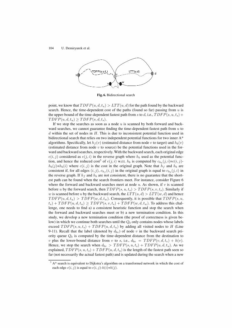
Fig. 6. Bidirectional search
point, we know that TDFP (u, d, tu) > LTT (u, d) for the path found by the backwardsearch. Hence, the time-dependent cost of the paths (found so far) passing from u isthe upper-bound of the time-dependent fastest path from s to d, i.e., TDFP (s, u, ts)+TDFP (u, d, tu) ≥ TDFP (s, d, ts).
If we stop the searches as soon as a node u is scanned by both forward and back-ward searches, we cannot guarantee finding the time-dependent fastest path from u tod within the set of nodes in H . This is due to inconsistent potential function used inbidirectional search that relies on two independent potential functions for two inner A*algorithms. Specifically, let hf (v) (estimated distance from node v to target) and hb(v)(estimated distance from node v to source) be the potential functions used in the for-ward and backward searches, respectively. With the backward search, each original edgee(i, j) considered as e(j, i) in the reverse graph where hb used as the potential func-tion, and hence the reduced cost3 of e(j, i) w.r.t. hb is computed by chb
(j, i)=c(i, j)-hb(j)+hb(i) where c(i, j) is the cost in the original graph. Note that hf and hb areconsistent if, for all edges (i, j), chf
(i, j) in the original graph is equal to chb(j, i) in
the reverse graph. If hf and hb are not consistent, there is no guarantee that the short-est path can be found when the search frontiers meet. For instance, consider Figure 6where the forward and backward searches meet at node u. As shown, if v is scannedbefore u by the forward search, then TDFP (s, u, ts) > TDFP (s, v, ts). Similarly ifw is scanned before u by the backward search, the LTT (u, d) > LTT (w, d) and henceTDFP (u, d, tu) > TDFP (w, d, tw). Consequently, it is possible that TDFP (s, u,ts) + TDFP (u, d, tu) ≥ TDFP (s, v, ts) + TDFP (w, d, tw). To address this chal-lenge, one needs to find a) a consistent heuristic function and stop the search whenthe forward and backward searches meet or b) a new termination condition. In thisstudy, we develop a new termination condition (the proof of correctness is given be-low) in which we continue both searches until the Qb only contains nodes whose labelsexceed TDFP (s, u, ts) + TDFP (u, d, tu) by adding all visited nodes to H (Line9-11). Recall that the label (denoted by dbv) of node v in the backward search pri-ority queue Qb is computed by the time-dependent distance from the destination tov plus the lower-bound distance from v to s, i.e., dbv = TDFP (v, d, tv) + h(v).Hence, we stop the search when dbv > TDFP (s, u, ts) + TDFP (u, d, tu). As weexplained, TDFP (s, u, ts) + TDFP (u, d, tu) is the length of the fastest path seen sofar (not necessarily the actual fastest path) and is updated during the search when a new
3 A* search is equivalent to Dijkstra’s algorithm on a transformed network in which the cost ofeach edge c(i, j) is equal to c(i, j)-h(i)+h(j).
Online Computation of Fastest Path in Time-Dependent Spatial Networks 105
common node u′ found with TDFP (s, u′, ts)+TDFP (u′, d, tu′) < TDFP (s, u, ts)+TDFP (u, d, tu). Once both searches stop, H will include all the candidate nodes thatcan possibly be part of the time-dependent fastest path to d. Finally, we continue theforward search considering only the nodes in H until we reach d (Line 12).
Algorithm 1. B-TDFP Algorithm
1: //Input: GT ,←−G , s:source, d:destination,ts:departure time
2: //Output: a (s, d, ts) fastest path3: //FS():forward search, BS():backward search, Nf /Nb: nodes scanned by FS()/BS(),
dbv:label of the minimum element in BS queue4: FS(GT ) and BS(
←−G) //start searches simultaneously
5: Nf ← FS(GT ) and Nb ← BS(←−G)
6: If Nf ∩Nb �= ∅ then u← Nf ∩Nb
7: M = TDFP (s, u, ts) + TDFP (u, d, tu)8: end If9: While dbv > M
10: Nb ← BS(←−G)
11: End While12: FS(Nb)13: return (s, d, ts)
Lemma 2. Algorithm 1 finds the correct time-dependent fastest path from source todestination for a given departure-time ts.
Proof. We prove Lemma 2 by contradiction. The forward search in Algorithm 1 is thesame as the unidirectional A* algorithm and our heuristic function h(v) is a lower-bound of time-dependent distance from u to v. Therefore, the forward search is correct.Now, let P (s, (u), d, ts) represent the path from s to d passing from u where forwardand backward searches meet and ω denotes the cost of this path. As we showed ω is theupper-bound of actual time-dependent fastest path from s to d. Let φ be the smallestlabel of the backward search in priority queue Qb when both forward and backwardsearches stopped. Recall that we stop searches when φ > ω. Suppose that Algorithm1 is not correct and yields a suboptimal path, i.e., the fastest path passes from a nodeoutside of the corridor generated by the forward and backward searches. Let P∗ be thefastest path from s to d for departure-time ts and cost of this path is α. Let v be the firstnode on P∗ which is going to be explored by the forward search and not explored bythe backward search and hb(v) is the heuristic function for the backward search. Hence,we have φ ≤ hb(v) + LTT (v, d), α ≤ ω < φ and hb(v) + LTT (v, d) ≤ LTT (s, v)+LTT (v, d) ≤ TDFP (s, v, ts)+TDFP (v, t, tv) = α, which is a contradiction. Hence,the fastest path will be found in the corridor of the nodes labeled by the backwardsearch.
6 Experimental Evaluation
6.1 Experimental Setup
We conducted extensive experiments with different spatial networks to evaluate the per-formance of our proposed bidirectional time-dependent fastest path (B-TDFP)
106 U. Demiryurek et al.
approach. As of our dataset, we used California (CA), Los Angeles (LA) and SanJoaquin County (SJ) road network data (obtained from Navteq [22]) with approxi-mately 1,965,300, 304,162 and 24,123 nodes, respectively. We conducted our experi-ments on a server with 2.7 GHz Pentium Core Duo processor with 12GB RAM memory.
6.1.1 Time-Dependent Network ModelingAt our research center, we maintain a very large-scale and high resolution (both spa-tial and temporal) traffic sensor (i.e., loop detector) dataset collected from entire LACounty highways and arterial streets. This dataset includes both inventory and real-timedata for 6300 traffic sensors covering approximately 3000 miles. The sampling rate ofthe streaming data is 1 reading/sensor/min. We have been continuously collecting andarchiving the traffic sensor data for the past two years. We use this real-world datasetto create time varying edge weights; we spatially and temporally aggregate sensor databy assigning interpolation points (for each 5 minutes) that depict the travel-times on thenetwork segments. Based on our observation, all roads are un-congested between 9PMand 6AM, and hence we assume static edge weights during this interval. In order tocreate time-dependent edge weights for the local streets in LA, CA and SJ, we devel-oped a traffic modeling approach [8] that synthetically generates the edge travel-timeprofiles. Our approach uses spatial (e.g., locality, connectivity) and temporal (e.g., rushhour, weekday) characteristics to generate travel-time for network edges that does nothave readily available sensor data.
6.2 Results
In this section, we report the experimental results from our fastest path queries in whichwe determine the s and d nodes uniformly at random. We also pick our departure-time randomly and uniformly distributed in time domain T . The average results arederived from 1000 random s-d queries. We only present the results for LA and CA, theexperimental results for both SJ and LA are very similar.
6.2.1 Comparison with ALTIn this set of experiments we compare our algorithm with time-dependent ALT (TD-ALT) approaches [6,21] with respect to storage and response time. We run our proposedalgorithm both unidirectionally and bidirectionally (in CA network) and compare with[6] and [21], respectively. As we mentioned, selecting good landmarks that lead to goodperformance is very difficult and hence several heuristics have been proposed for land-mark selection. Among these heuristics, we use the best known technique; maxCover(see [6]) with 64 landmarks. We computed travel-times between each node and thelandmarks with respect to G. Under this setting, to store the precomputed distances,TD-ALT attaches to each node an array of 64 elements corresponding to the number oflandmarks. Assuming that each array element takes 2 bytes of space, the additional stor-age requirement of TD-ALT is 63 Megabytes. On the other hand, with our algorithm,we divide CA network to 60 partitions and store the intra and inter distance labels. Thetotal storage requirement of our proposed solution is 8.5 Megabytes where we con-sume, for each node, an array of 2 elements (corresponding to from and to distances
Online Computation of Fastest Path in Time-Dependent Spatial Networks 107
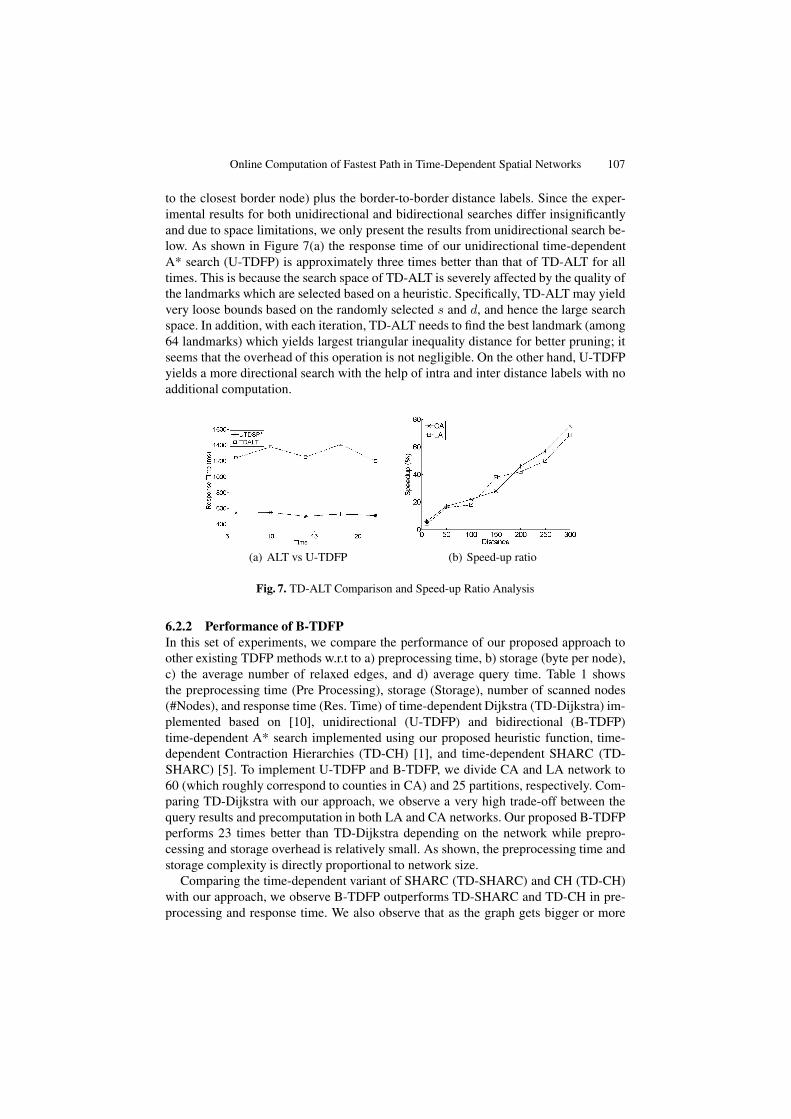
to the closest border node) plus the border-to-border distance labels. Since the exper-imental results for both unidirectional and bidirectional searches differ insignificantlyand due to space limitations, we only present the results from unidirectional search be-low. As shown in Figure 7(a) the response time of our unidirectional time-dependentA* search (U-TDFP) is approximately three times better than that of TD-ALT for alltimes. This is because the search space of TD-ALT is severely affected by the quality ofthe landmarks which are selected based on a heuristic. Specifically, TD-ALT may yieldvery loose bounds based on the randomly selected s and d, and hence the large searchspace. In addition, with each iteration, TD-ALT needs to find the best landmark (among64 landmarks) which yields largest triangular inequality distance for better pruning; itseems that the overhead of this operation is not negligible. On the other hand, U-TDFPyields a more directional search with the help of intra and inter distance labels with noadditional computation.
(a) ALT vs U-TDFP (b) Speed-up ratio
Fig. 7. TD-ALT Comparison and Speed-up Ratio Analysis
6.2.2 Performance of B-TDFPIn this set of experiments, we compare the performance of our proposed approach toother existing TDFP methods w.r.t to a) preprocessing time, b) storage (byte per node),c) the average number of relaxed edges, and d) average query time. Table 1 showsthe preprocessing time (Pre Processing), storage (Storage), number of scanned nodes(#Nodes), and response time (Res. Time) of time-dependent Dijkstra (TD-Dijkstra) im-plemented based on [10], unidirectional (U-TDFP) and bidirectional (B-TDFP)time-dependent A* search implemented using our proposed heuristic function, time-dependent Contraction Hierarchies (TD-CH) [1], and time-dependent SHARC (TD-SHARC) [5]. To implement U-TDFP and B-TDFP, we divide CA and LA network to60 (which roughly correspond to counties in CA) and 25 partitions, respectively. Com-paring TD-Dijkstra with our approach, we observe a very high trade-off between thequery results and precomputation in both LA and CA networks. Our proposed B-TDFPperforms 23 times better than TD-Dijkstra depending on the network while prepro-cessing and storage overhead is relatively small. As shown, the preprocessing time andstorage complexity is directly proportional to network size.
Comparing the time-dependent variant of SHARC (TD-SHARC) and CH (TD-CH)with our approach, we observe B-TDFP outperforms TD-SHARC and TD-CH in pre-processing and response time. We also observe that as the graph gets bigger or more

108 U. Demiryurek et al.
Table 1. Experimental Results
Algorithm PreProcessing Storage #Nodes Res. Time[h:m] [B/node] [ms]
CA
TD-Dijkstra 0:00 0 1162323 4104.11
U-TDFP 1:13 6.82 90575 310.17
B-TDFP 1:13 6.82 67172 182.06
TD-SHARC 19:41 154.10 75104 227.26
TD-CH 3:55 1018.33 70011 209.12
LA
TD-Dijkstra 0:00 0 210384 2590.07
U-TDFP 0:27 3.51 11115 197.23
B-TDFP 0:27 3.51 6681 101.22
TD-SHARC 11:12 68.47 9566 168.11
TD-CH 1:58 740.88 7922 140.25
edges are time-dependent, the preprocessing time of TD-SHARC increases drastically.The preprocessing of TD-SHARC takes very long for both road networks, i.e., up to20 times more than B-TDFP. The reason for the performance gap is that TD-SHARC’scontraction routine cannot bypass the majority of the nodes in time-dependent road net-works as in the static road networks. Recall that the importance of a node can changethroughout the time under consideration in time-dependent road networks. In addition,TD-SHARC is very sensitive to edge cost function changes, i.e. whenever cost func-tion of an edge changes, the preprocessing phase needs to be repeated to determine theby-pass nodes. While TD-CH tend to have better response times than TD-SHARC, thespace consumption of TD-CH is significantly high (approximately 1000 bytes per nodein CA network). For this reason, TD-CH is not feasible for very large road networkssuch as North America and Europe. We note that, to improve the response and prepro-cessing time, several variations of TD-SHARC and TD-CH algorithms are implementedin the literature. These variations trade-off between the optimality of the solution andthe response time. For example, the response time of Heuristic TD-SHARC [5] is shownmuch better than that of original TD-SHARC algorithm. However, the path found bythe Heuristic TD-SHARC is not optimal and the error rate is not bounded. As anotherexample, the performance of TD-SHARC can be improved by combining with anothertechnique called Arc-Flags [5]. Similar performance improvements can be applied toour proposed approach. For instance, we can terminate the search when the search fron-tiers meet and report the combination of path found by the forward and backward searchas the result. However, as mentioned in Section 5.2, we cannot guarantee the optimalsolution in this setting. Moreover, based on our initial observation and implementation,we can also integrate our algorithm with Arc-Flags. However, the focus of our study isto develop a technique that yields exact solutions. Hence, for the sake of simplicity and
Online Computation of Fastest Path in Time-Dependent Spatial Networks 109
fair comparison, we only compare the original algorithms that yields exact results anddo not consider integrating different methods.
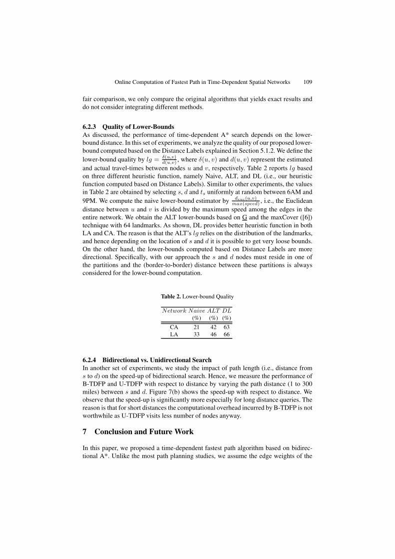
6.2.3 Quality of Lower-BoundsAs discussed, the performance of time-dependent A* search depends on the lower-bound distance. In this set of experiments, we analyze the quality of our proposed lower-bound computed based on the Distance Labels explained in Section 5.1.2. We define thelower-bound quality by lg = δ(u,v)
d(u,v) , where δ(u, v) and d(u, v) represent the estimatedand actual travel-times between nodes u and v, respectively. Table 2 reports lg basedon three different heuristic function, namely Naive, ALT, and DL (i.e., our heuristicfunction computed based on Distance Labels). Similar to other experiments, the valuesin Table 2 are obtained by selecting s, d and ts uniformly at random between 6AM and9PM. We compute the naive lower-bound estimator by deuc(u,v)
max(speed) , i.e., the Euclideandistance between u and v is divided by the maximum speed among the edges in theentire network. We obtain the ALT lower-bounds based on G and the maxCover ([6])technique with 64 landmarks. As shown, DL provides better heuristic function in bothLA and CA. The reason is that the ALT’s lg relies on the distribution of the landmarks,and hence depending on the location of s and d it is possible to get very loose bounds.On the other hand, the lower-bounds computed based on Distance Labels are moredirectional. Specifically, with our approach the s and d nodes must reside in one ofthe partitions and the (border-to-border) distance between these partitions is alwaysconsidered for the lower-bound computation.
Table 2. Lower-bound Quality
Network Naive ALT DL(%) (%) (%)
CA 21 42 63LA 33 46 66
6.2.4 Bidirectional vs. Unidirectional SearchIn another set of experiments, we study the impact of path length (i.e., distance froms to d) on the speed-up of bidirectional search. Hence, we measure the performance ofB-TDFP and U-TDFP with respect to distance by varying the path distance (1 to 300miles) between s and d. Figure 7(b) shows the speed-up with respect to distance. Weobserve that the speed-up is significantly more especially for long distance queries. Thereason is that for short distances the computational overhead incurred by B-TDFP is notworthwhile as U-TDFP visits less number of nodes anyway.
7 Conclusion and Future Work
In this paper, we proposed a time-dependent fastest path algorithm based on bidirec-tional A*. Unlike the most path planning studies, we assume the edge weights of the

110 U. Demiryurek et al.
road network are time varying rather than constant. Therefore, our approach yield amuch more realistic scenario, and hence, applicable to the to real-world road networks.We also compared our approaches with those handful of time-dependent fastest pathstudies. Our experiments with real-world road network and traffic data showed that ourproposed approaches outperform the competitors in storage and response time signifi-cantly. We intend to pursue this study in two different directions. First, we plan to in-vestigate new data models for effective representation of spatiotemporal road networks.This is critical in supporting development of efficient and accurate time-dependent al-gorithms, while minimizing the storage and computation costs. Second, to support rapidchanges of the traffic patterns (that may happen in case of accidents/events, for exam-ple), we intend to study incremental update algorithms for both of our approaches.
References
1. Batz, G.V., Delling, D., Sanders, P., Vetter, C.: Time-dependent contraction hierarchies. In:ALENEX (2009)
2. Cooke, L., Halsey, E.: The shortest route through a network with timedependent internodaltransit times. Journal of Mathematical Analysis and Applications (1966)
3. Dean, B.C.: Algorithms for min-cost paths in time-dependent networks with wait policies.Networks (2004)
4. Dehne, F., Omran, M.T., Sack, J.-R.: Shortest paths in time-dependent fifo networks usingedge load forecasts. In: IWCTS (2009)
5. Delling, D.: Time-dependent SHARC-routing. In: Halperin, D., Mehlhorn, K. (eds.) Esa2008. LNCS, vol. 5193, pp. 332–343. Springer, Heidelberg (2008)
6. Delling, D., Wagner, D.: Landmark-based routing in dynamic graphs. In: Demetrescu, C.(ed.) WEA 2007. LNCS, vol. 4525, pp. 52–65. Springer, Heidelberg (2007)
7. Demiryurek, U., Kashani, F.B., Shahabi, C.: A case for time-dependent shortest path compu-tation in spatial networks. In: ACM SIGSPATIAL (2010)
8. Demiryurek, U., Pan, B., Kashani, F.B., Shahabi, C.: Towards modeling the traffic data onroad networks. In: SIGSPATIAL-IWCTS (2009)
9. Ding, B., Yu, J.X., Qin, L.: Finding time-dependent shortest paths over large graphs. In:EDBT (2008)
10. Dreyfus, S.E.: An appraisal of some shortest-path algorithms. Operations Research 17(3)(1969)
11. Foschini, L., Hershberger, J., Suri, S.: On the complexity of time-dependent shortest paths.In: SODA (2011)
12. George, B., Kim, S., Shekhar, S.: Spatio-temporal network databases and routing algorithms:A summary of results. In: Papadias, D., Zhang, D., Kollios, G. (eds.) SSTD 2007. LNCS,vol. 4605, pp. 460–477. Springer, Heidelberg (2007)
13. Goldberg, A.V., Harellson, C.: Computing the shortest path: A* search meets graph theory.In: SODA (2005)
14. Gonzalez, H., Han, J., Li, X., Myslinska, M., Sondag, J.P.: Adaptive fastest path computationon a road network: A traffic mining approach. In: VLDB (2007)
15. Guc, B., Ranganathan, A.: Real-time, scalable route planning using stream-processing in-frastructure. In: ITS (2010)
16. Halpern, J.: Shortest route with time dependent length of edges and limited delay possibilitiesin nodes. Mathematical Methods of Operations Research (1969)
17. Hart, P., Nilsson, N., Raphael, B.: A formal basis for the heuristic determination of minimumcost paths. IEEE Transactions on Systems Science and Cybernetics (1968)
Online Computation of Fastest Path in Time-Dependent Spatial Networks 111
18. Kanoulas, E., Du, Y., Xia, T., Zhang, D.: Finding fastest paths on a road network with speedpatterns. In: ICDE (2006)
19. Kohler, E., Langkau, K., Skutella, M.: Time-expanded graphs for flow-dependent transittimes. In: Proc. 10th Annual European Symposium on Algorithms (2002)
20. Kolahdouzan, M., Shahabi, C.: Voronoi-based k nearest neighbor search for spatial networkdatabases. In: VLDB (2004)
21. Nannicini, G., Delling, D., Liberti, L., Schultes, D.: Bidirectional a* search for time-dependent fast paths. In: McGeoch, C.C. (ed.) WEA 2008. LNCS, vol. 5038, pp. 334–346.Springer, Heidelberg (2008)
22. NAVTEQ, http://www.navteq.com (accessed in May 2010)23. Orda, A., Rom, R.: Shortest-path and minimum-delay algorithms in networks with time-
dependent edge-length. J. ACM (1990)24. PeMS, https://pems.eecs.berkeley.edu (accessed in May 2010)25. Pohl, I.: Bi-directional search. In: Machine Intelligence. Edinburgh University Press, Edin-
burgh (1971)26. Potamias, M., Bonchi, F., Castillo, C., Gionis, A.: Fast shortest path distance estimation in
large networks. In: CIKM (2009)27. Samet, H., Sankaranarayanan, J., Alborzi, H.: Scalable network distance browsing in spatial
databases. In: SIGMOD (2008)28. Sanders, P., Schultes, D.: Highway hierarchies hasten exact shortest path queries. In: Brodal,
G.S., Leonardi, S. (eds.) ESA 2005. LNCS, vol. 3669, pp. 568–579. Springer, Heidelberg(2005)
29. Sanders, P., Schultes, D.: Engineering fast route planning algorithms. In: Demetrescu, C.(ed.) WEA 2007. LNCS, vol. 4525, pp. 23–36. Springer, Heidelberg (2007)
30. TELEATLAS, http://www.teleatlas.com (accessed in May 2010)31. Wagner, D., Willhalm, T.: Geometric speed-up techniques for finding shortest paths in large
sparse graphs. In: Di Battista, G., Zwick, U. (eds.) ESA 2003. LNCS, vol. 2832, pp. 776–787.Springer, Heidelberg (2003)