Online Appendix

Pierre Dubois, Rachel Griffith and Martin O’Connell

How well targeted are soda taxes?

American Economic Review

A Data appendix

A.1 Patterns of sugar consumption

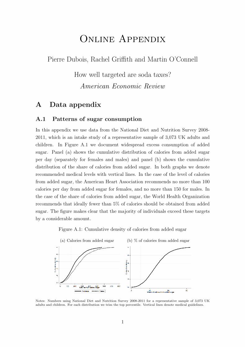
In this appendix we use data from the National Diet and Nutrition Survey 2008-

2011, which is an intake study of a representative sample of 3,073 UK adults and

children. In Figure A.1 we document widespread excess consumption of added

sugar. Panel (a) shows the cumulative distribution of calories from added sugar

per day (separately for females and males) and panel (b) shows the cumulative

distribution of the share of calories from added sugar. In both graphs we denote

recommended medical levels with vertical lines. In the case of the level of calories

from added sugar, the American Heart Association recommends no more than 100

calories per day from added sugar for females, and no more than 150 for males. In

the case of the share of calories from added sugar, the World Health Organization

recommends that ideally fewer than 5% of calories should be obtained from added

sugar. The figure makes clear that the majority of individuals exceed these targets

by a considerable amount.

Figure A.1: Cumulative density of calories from added sugar

(a) Calories from added sugar (b) % of calories from added sugar

Notes: Numbers using National Diet and Nutrition Survey 2008-2011 for a representative sample of 3,073 UKadults and children. For each distribution we trim the top percentile. Vertical lines denote medical guidelines.

1

In Figure A.2 we show local polynomial regressions describing how the calories

from (the sugar in) soft drinks vary with age, share of calories from added sugar

and equivalized household income. The figure shows that young individuals, those

with a high share of calories from added sugar, and those from relatively low income

households obtain relatively large amounts of calories from soft drinks.

Figure A.2: Sugar from soft drinks

(a) by age (b) by calories from added sugar

(c) by equivalized income

Notes: Numbers using National Diet and Nutrition Survey 2008-2011 for a representative sample of 3,073 UKadults and children. Lines are based on local polynomial regressions. Shaded area are 95% confidence bands. Foreach variable we trim the top percentile of the distribution.

In Figures A.3 and A.4 we repeat Figures A.1 and A.2 with US data. Specifically,

we use National Health and Nutrition Examination Study over 2007-2014, a sample

of 39,189 adults and children. The same patterns hold in the US. Notice, the level of

calories from soft drinks reported for the US in the National Health and Nutrition

Examination Study is higher than those reported in the UK in the National Diet

and Nutrition Survey. This may partially reflect differences in consumption levels

between the two countries, but it may also reflect differences in reporting between

the two surveys.

2

Figure A.3: Patterns in the US: Cumulative density of calories from added sugar

(a) Calories from added sugar (b) % of calories from added sugar

Notes: Numbers using National Health and Nutrition Examination Study 2007-2014 for a representative sampleof 39,189 US adults and children. For each distribution we trim the top percentile. Vertical lines denote medicalguidelines.

Figure A.4: Patterns in the US: Sugar from soft drinks

(a) by age (b) by calories from added sugar

(c) by equivalized income

Notes: Numbers using National Health and Nutrition Examination Study 2007-2014 for a representative sample of39,189 US adults and children. Lines are based on local polynomial regressions. Shaded area are 95% confidencebands. For each variable we trim the top percentile of the distribution.

3

A.2 Product definition

We consider the market for chilled non-alcoholic drinks. In the raw data there are

2,950 unique product codes (UPCs) consisting of 1,065 brands (as defined by Kan-

tar). We use data on the 598 UPCs in 89 brands that comprise 82% of transactions.

We drop niches UPCs that have very small market shares as follows:

• 975 brands that individually have a market share of less than 0.15%, ac-

counting for 2,232 UPCs. Together these account for 15% of the market; see

spreadsheet.

• 87 UPCs that are for sizes smaller than 200ml, which together account for 2%

of the market; see spreadsheet.

• 33 UPCs that are for odd size-brand combinations, that individually have

small market shares (the largest is 0.18%, the mean is 0.04%), which together

account for 1% of the market; see spreadsheet.

This leaves us with 598 UPCs in 89 brands. We group these into 37 products

as follows:

• 30 branded soft drink products, e.g. Coca Cola 330ml, Coca Cola 500ml, Coca

Cola Diet 330ml, etc.; we aggregate over 104 UPCs, for example, the product

Coca Cola 500ml is the aggregate of 2 UPCs that differ in the shape of bottle

(COCA COLA CONTOUR PET 500ML with a market share of 7.5% and

COCA COLA PET 500ML with a market share of 0.2%); together these 30

branded soft drink products account for 60% market share; see spreadsheet

• Other soda products

– regular: we aggregate 184 UPCs that individually have market shares

that range from 1.6% (Red Bull 250ml) to 0.0002% (Orangina Rouge

500ml) with a mean market share of 0.08%, and together account for

14% of the market; see spreadsheet.

– diet: we aggregate 22 UPCs that individually have market shares that

range from 0.4% (7UP Free Lemon+Limeade 600ml) to 0.001% (Lu-

cozade Sport Lite 500ml) and together account for 1.9% of the market;

see spreadsheet.

• Fruit juice: we aggregate 100 UPCs that individually all have market shares

below 1% and together account for 7.9% of the market; see spreadsheet.

4

• Flavoured milk: we aggregate 30 UPCs that individually have market shares

below 0.25% and together account for 1.8% of the market; see spreadsheet.

• Fruit water: we aggregate 11 UPCs that are different flavours of Volvic Touch

of Fruit Water that together account for just under 1% of the market; see

spreadsheet.

• Water: we aggregate 146 UPCs for bottled water, which together have a

market share of 12%; see spreadsheet.

A.3 Measurement of prices

We compute the transaction level price as expenditure made for a UPC over units

purchased. For products that entail some aggregation over sizes, we adjust prices

so they are in terms of the most popular size. For instance, Pepsi 500ml involves

aggregating over 500ml and 600ml size; for transactions involving 600ml Pepsi, we

adjust the price according to p ∗ 5/6. Similarly, for the composite products we

express price in terms of the most common size.

For each product we compute the mean monthly price (across transactions) in

each retailer type. If a product-retailer type-month involves fewer than 3 transac-

tions, we replace the price with a missing value. For product-retailer type-months

with missing prices we interpolate (across weeks). We smooth the resulting price

series using a local polynomial non-parametric regression.

Figures A.5 and A.6 show the difference between the price the consumer actually

pays for the chosen product (the transaction price) and the smoothed price used in

the demand model estimation. They show that measurement error exists and exists

for all stores and if anything is slightly lower for vending machines.

Figure A.5: Difference between transaction price and smoothed price

Notes: .

5

Figure A.6: Difference between transaction price and smoothed price, by store type

(a) National-large (b) National-small (c) Vending machine

(d) Regional - south (e) Regional - midlands (f) Regional - north

Notes: .

Measurement error in non-linear models is more problematic than in linear mod-

els, and even classical additive measurement error can bias parameter estimates,

unlike in linear models. However, it is useful to consider more closely the type

of measurement error we face here. The measurement errors introduced by using

imputed prices instead of true prices can be thought of coming from two errors.

First, there is an error when using a mean instead of the true variable. These errors

are “Berkson” errors (Berkson (1950)), i.e. additive on the unobserved true price

and independent of the average price used in estimation. Second, we also make an

error on the true mean price in a region-store chain when using transaction prices

because the sampling of transactions is not independent of prices.

Blundell, Horowtiz and Parey (2019) argue that “Berkson” errors are common-

place when we observe an average price in a group rather than the true individual

price, and can lead to bias in estimates of demand. They are not classical mea-

surement errors independent of the true unobserved variable. Schennach (2013)

proposes a solution with instrumental variables in the context of non-parametric

models with a continuous outcome variable. In a continuous demand estimation

problem, Blundell, Horowtiz and Parey (2019) develop a consistent estimator that

uses external information on the true distribution of prices in the case of demand es-

timation with non-separable unobserved heterogeneity. Their results do not extend

to a discrete choice model for differentiated products demands.

The second source of errors is due to the imputation using transaction prices.

6

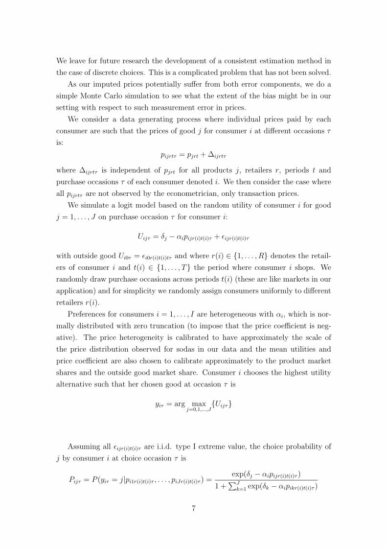
We leave for future research the development of a consistent estimation method in

the case of discrete choices. This is a complicated problem that has not been solved.

As our imputed prices potentially suffer from both error components, we do a

simple Monte Carlo simulation to see what the extent of the bias might be in our

setting with respect to such measurement error in prices.

We consider a data generating process where individual prices paid by each

consumer are such that the prices of good j for consumer i at different occasions τ

is:

pijrtτ = pjrt + ∆ijrtτ

where ∆ijrtτ is independent of pjrt for all products j, retailers r, periods t and

purchase occasions τ of each consumer denoted i. We then consider the case where

all pijrtτ are not observed by the econometrician, only transaction prices.

We simulate a logit model based on the random utility of consumer i for good

j = 1, . . . , J on purchase occasion τ for consumer i:

Uijτ = δj − αipijr(i)t(i)τ + εijr(i)t(i)τ

with outside good Ui0τ = εi0r(i)t(i)tτ and where r(i) ∈ 1, . . . , R denotes the retail-

ers of consumer i and t(i) ∈ 1, . . . , T the period where consumer i shops. We

randomly draw purchase occasions across periods t(i) (these are like markets in our

application) and for simplicity we randomly assign consumers uniformly to different

retailers r(i).

Preferences for consumers i = 1, . . . , I are heterogeneous with αi, which is nor-

mally distributed with zero truncation (to impose that the price coefficient is neg-

ative). The price heterogeneity is calibrated to have approximately the scale of

the price distribution observed for sodas in our data and the mean utilities and

price coefficient are also chosen to calibrate approximately to the product market

shares and the outside good market share. Consumer i chooses the highest utility

alternative such that her chosen good at occasion τ is

yiτ = arg maxj=0,1,...,J

Uijτ

Assuming all εijr(i)t(i)τ are i.i.d. type I extreme value, the choice probability of

j by consumer i at choice occasion τ is

Pijτ = P (yiτ = j|pi1r(i)t(i)τ , . . . , piJr(i)t(i)τ ) =exp(δj − αipijr(i)t(i)τ )

1 +∑J

k=1 exp(δk − αipikr(i)t(i)τ )

7

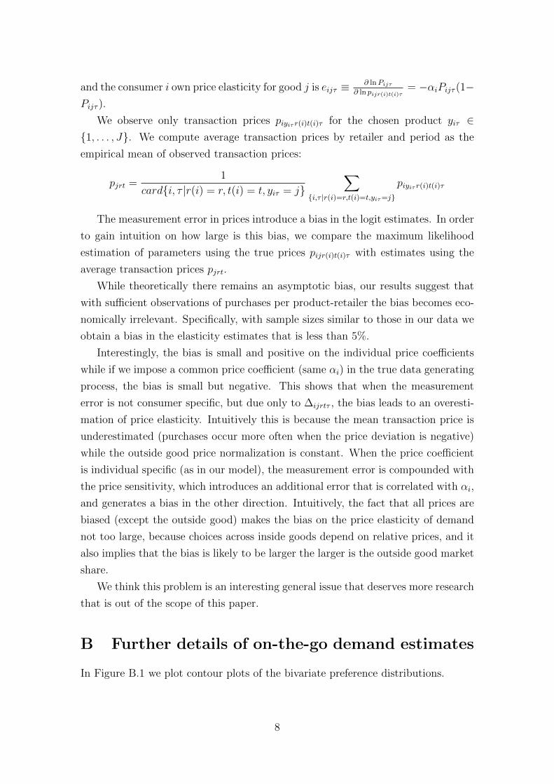
and the consumer i own price elasticity for good j is eijτ ≡ ∂ lnPijτ∂ ln pijr(i)t(i)τ

= −αiPijτ (1−Pijτ ).

We observe only transaction prices piyiτ r(i)t(i)τ for the chosen product yiτ ∈1, . . . , J. We compute average transaction prices by retailer and period as the

empirical mean of observed transaction prices:

pjrt =1

cardi, τ |r(i) = r, t(i) = t, yiτ = j∑

i,τ |r(i)=r,t(i)=t,yiτ=j

piyiτ r(i)t(i)τ

The measurement error in prices introduce a bias in the logit estimates. In order

to gain intuition on how large is this bias, we compare the maximum likelihood

estimation of parameters using the true prices pijr(i)t(i)τ with estimates using the

average transaction prices pjrt.

While theoretically there remains an asymptotic bias, our results suggest that

with sufficient observations of purchases per product-retailer the bias becomes eco-

nomically irrelevant. Specifically, with sample sizes similar to those in our data we

obtain a bias in the elasticity estimates that is less than 5%.

Interestingly, the bias is small and positive on the individual price coefficients

while if we impose a common price coefficient (same αi) in the true data generating

process, the bias is small but negative. This shows that when the measurement

error is not consumer specific, but due only to ∆ijrtτ , the bias leads to an overesti-

mation of price elasticity. Intuitively this is because the mean transaction price is

underestimated (purchases occur more often when the price deviation is negative)

while the outside good price normalization is constant. When the price coefficient

is individual specific (as in our model), the measurement error is compounded with

the price sensitivity, which introduces an additional error that is correlated with αi,

and generates a bias in the other direction. Intuitively, the fact that all prices are

biased (except the outside good) makes the bias on the price elasticity of demand

not too large, because choices across inside goods depend on relative prices, and it

also implies that the bias is likely to be larger the larger is the outside good market

share.

We think this problem is an interesting general issue that deserves more research

that is out of the scope of this paper.

B Further details of on-the-go demand estimates

In Figure B.1 we plot contour plots of the bivariate preference distributions.

8

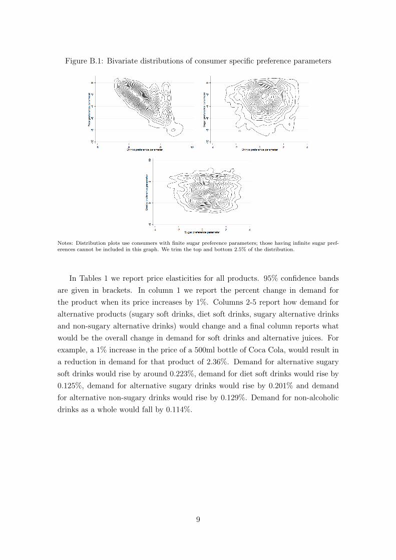
Figure B.1: Bivariate distributions of consumer specific preference parameters

Notes: Distribution plots use consumers with finite sugar preference parameters; those having infinite sugar pref-erences cannot be included in this graph. We trim the top and bottom 2.5% of the distribution.

In Tables 1 we report price elasticities for all products. 95% confidence bands

are given in brackets. In column 1 we report the percent change in demand for

the product when its price increases by 1%. Columns 2-5 report how demand for

alternative products (sugary soft drinks, diet soft drinks, sugary alternative drinks

and non-sugary alternative drinks) would change and a final column reports what

would be the overall change in demand for soft drinks and alternative juices. For

example, a 1% increase in the price of a 500ml bottle of Coca Cola, would result in

a reduction in demand for that product of 2.36%. Demand for alternative sugary

soft drinks would rise by around 0.223%, demand for diet soft drinks would rise by

0.125%, demand for alternative sugary drinks would rise by 0.201% and demand

for alternative non-sugary drinks would rise by 0.129%. Demand for non-alcoholic

drinks as a whole would fall by 0.114%.

9

Table 1: Product level price elasticities

Effect of 1% price increase on:Own cross demand for: Total

product sugary diet sugary non-sugary drinksdemand soft drinks soft drinks alternatives alternatives demand

Coca Cola 330 -2.81 0.096 0.055 0.084 0.092 -0.012[-2.85, -2.80] [0.095, 0.098] [0.054, 0.056] [0.083, 0.086] [0.091, 0.094] [-0.012, -0.012]

Coca Cola 500 -2.36 0.223 0.125 0.201 0.129 -0.114[-2.38, -2.30] [0.218, 0.225] [0.122, 0.126] [0.196, 0.203] [0.126, 0.131] [-0.114, -0.111]

Coca Cola Diet 330 -3.02 0.047 0.106 0.036 0.232 -0.004[-3.05, -3.00] [0.046, 0.048] [0.104, 0.107] [0.035, 0.036] [0.228, 0.235] [-0.005, -0.004]

Coca Cola Diet 500 -2.51 0.100 0.235 0.098 0.224 -0.084[-2.53, -2.47] [0.098, 0.102] [0.229, 0.239] [0.095, 0.100] [0.221, 0.228] [-0.085, -0.082]

Dr Pepper 330 -3.25 0.014 0.007 0.007 0.009 -0.001[-3.30, -3.23] [0.014, 0.015] [0.007, 0.008] [0.007, 0.008] [0.009, 0.010] [-0.002, -0.001]

Dr Pepper 500 -2.64 0.035 0.020 0.031 0.020 -0.018[-2.66, -2.59] [0.034, 0.036] [0.019, 0.020] [0.030, 0.031] [0.020, 0.021] [-0.018, -0.017]

Dr Pepper Diet 500 -2.85 0.016 0.038 0.015 0.038 -0.013[-2.88, -2.80] [0.016, 0.016] [0.037, 0.039] [0.014, 0.015] [0.037, 0.039] [-0.013, -0.013]

Fanta 330 -2.99 0.020 0.010 0.015 0.018 -0.002[-3.04, -2.97] [0.020, 0.020] [0.010, 0.010] [0.014, 0.015] [0.018, 0.019] [-0.003, -0.002]

Fanta 500 -2.54 0.036 0.020 0.033 0.023 -0.019[-2.57, -2.49] [0.035, 0.037] [0.020, 0.021] [0.032, 0.034] [0.022, 0.023] [-0.019, -0.018]

Fanta Diet 500 -2.74 0.016 0.038 0.016 0.041 -0.014[-2.77, -2.70] [0.016, 0.017] [0.036, 0.038] [0.016, 0.017] [0.040, 0.042] [-0.014, -0.014]

Cherry Coke 330 -2.99 0.014 0.006 0.009 0.011 -0.001[-3.03, -2.97] [0.014, 0.015] [0.006, 0.007] [0.009, 0.009] [0.010, 0.011] [-0.001, -0.001]

Cherry Coke 500 -2.59 0.029 0.016 0.027 0.018 -0.015[-2.61, -2.53] [0.029, 0.030] [0.016, 0.016] [0.026, 0.027] [0.017, 0.018] [-0.015, -0.014]

Cherry Coke Diet 500 -2.79 0.013 0.030 0.013 0.032 -0.011[-2.81, -2.74] [0.013, 0.013] [0.029, 0.031] [0.012, 0.013] [0.031, 0.033] [-0.011, -0.011]

Oasis 500 -2.55 0.044 0.025 0.041 0.027 -0.023[-2.58, -2.49] [0.043, 0.045] [0.024, 0.026] [0.040, 0.042] [0.026, 0.027] [-0.023, -0.022]

Oasis Diet 500 -2.72 0.020 0.047 0.020 0.047 -0.017[-2.74, -2.68] [0.020, 0.020] [0.046, 0.048] [0.019, 0.020] [0.046, 0.048] [-0.017, -0.017]

Pepsi 330 -2.80 0.035 0.018 0.030 0.034 -0.004[-2.84, -2.79] [0.035, 0.036] [0.018, 0.019] [0.029, 0.030] [0.034, 0.036] [-0.005, -0.004]

Pepsi 500 -2.67 0.091 0.051 0.079 0.061 -0.050[-2.70, -2.64] [0.090, 0.093] [0.049, 0.052] [0.078, 0.081] [0.060, 0.062] [-0.050, -0.049]

Pepsi Diet 330 -3.06 0.016 0.043 0.012 0.089 -0.001[-3.09, -3.04] [0.016, 0.016] [0.042, 0.044] [0.012, 0.013] [0.087, 0.091] [-0.002, -0.001]

Pepsi Diet 500 -2.86 0.042 0.100 0.038 0.119 -0.038[-2.89, -2.83] [0.041, 0.042] [0.098, 0.101] [0.037, 0.039] [0.117, 0.121] [-0.038, -0.037]

Lucozade Energy 380 -2.72 0.053 0.029 0.052 0.040 -0.012[-2.76, -2.69] [0.052, 0.055] [0.028, 0.030] [0.051, 0.054] [0.039, 0.041] [-0.012, -0.012]

Lucozade Energy 500 -2.58 0.043 0.024 0.040 0.024 -0.022[-2.60, -2.52] [0.041, 0.044] [0.023, 0.025] [0.038, 0.041] [0.023, 0.025] [-0.022, -0.021]

Ribena 288 -2.87 0.015 0.008 0.012 0.016 0.000[-2.92, -2.85] [0.015, 0.016] [0.007, 0.008] [0.012, 0.013] [0.015, 0.016] [0.000, 0.000]

Ribena 500 -2.64 0.026 0.014 0.024 0.017 -0.013[-2.66, -2.59] [0.025, 0.026] [0.014, 0.014] [0.023, 0.025] [0.016, 0.017] [-0.014, -0.013]

Ribena Diet 500 -2.80 0.011 0.026 0.011 0.031 -0.010[-2.82, -2.76] [0.011, 0.012] [0.025, 0.026] [0.011, 0.012] [0.030, 0.032] [-0.010, -0.010]

Sprite 330 -3.25 0.012 0.007 0.008 0.009 -0.001[-3.30, -3.23] [0.012, 0.013] [0.007, 0.007] [0.008, 0.008] [0.009, 0.010] [-0.002, -0.001]

Sprite 500 -2.55 0.030 0.017 0.029 0.019 -0.016[-2.57, -2.49] [0.029, 0.031] [0.017, 0.018] [0.028, 0.030] [0.018, 0.020] [-0.016, -0.015]

Irn Bru 330 -2.94 0.009 0.004 0.007 0.008 -0.001[-2.99, -2.93] [0.009, 0.010] [0.004, 0.005] [0.007, 0.007] [0.008, 0.009] [-0.001, -0.001]

Irn Bru 500 -2.69 0.019 0.010 0.018 0.013 -0.010[-2.73, -2.65] [0.019, 0.020] [0.010, 0.011] [0.017, 0.018] [0.013, 0.014] [-0.010, -0.010]

Irn Bru Diet 330 -3.24 0.004 0.012 0.003 0.024 0.000[-3.28, -3.22] [0.004, 0.004] [0.012, 0.013] [0.003, 0.003] [0.023, 0.025] [0.000, 0.000]

Irn Bru Diet 500 -2.91 0.009 0.019 0.008 0.025 -0.007[-2.94, -2.88] [0.008, 0.009] [0.019, 0.020] [0.008, 0.009] [0.025, 0.026] [-0.008, -0.007]

Notes: For each of the four products listed we compute the change in demand for that product, for alternativesugary and diet options and for total demand resulting from a 1% price increase. Numbers are means across time.95% confidence intervals are shown in brackets. 10

Table 1 cont.

Effect of 1% price increase on:Own cross demand for: Total

product sugary diet sugary non-sugary drinksdemand soft drinks soft drinks alternatives alternatives demand

Other Diet -2.31 0.049 0.112 0.045 0.079 -0.034[-2.29, -2.17] [0.047, 0.049] [0.108, 0.114] [0.043, 0.045] [0.077, 0.080] [-0.034, -0.033]

Fruit juice -2.26 0.128 0.080 0.168 0.123 -0.012[-2.28, -2.22] [0.125, 0.130] [0.078, 0.081] [0.164, 0.171] [0.121, 0.125] [-0.012, -0.011]

Flavoured milk -2.66 0.035 0.018 0.035 0.029 -0.020[-2.69, -2.63] [0.035, 0.036] [0.018, 0.019] [0.034, 0.036] [0.028, 0.030] [-0.020, -0.019]

Fruit water -2.72 0.017 0.010 0.020 0.017 -0.011[-2.76, -2.69] [0.017, 0.018] [0.009, 0.010] [0.019, 0.020] [0.017, 0.018] [-0.011, -0.010]

Water -2.30 0.115 0.281 0.128 -0.141[-2.33, -2.28] [0.114, 0.118] [0.277, 0.284] [0.127, 0.131] [., .] [-0.144, -0.141]

Notes: For each of the four products listed we compute the change in demand for that product, for alternativesugary and diet options and for total demand resulting from a 1% price increase. Numbers are means across time.95% confidence intervals are shown in brackets.

In Figures B.2 and B.3 we replicate Figures 2 and 3, splitting individuals out

based on gender and in Figures B.4 and B.5 we split individuals out based on the

socioeconomic status. The graphs show the patterns of how preferences vary with

age and total dietary sugar broadly hold conditional on gender and socioeconomic

status.

Figure B.2: Preferences variation with age and gender

(a) price preferences (b) drink preferences

(c) infinite sugar preferences (d) finite sugar preferences

Notes: Figures show how the mean of price preferences, the mean of drinks preferences, the share of consumerswith infinite sugar preferences and the mean of finite sugar preferences vary by age and gender.

11

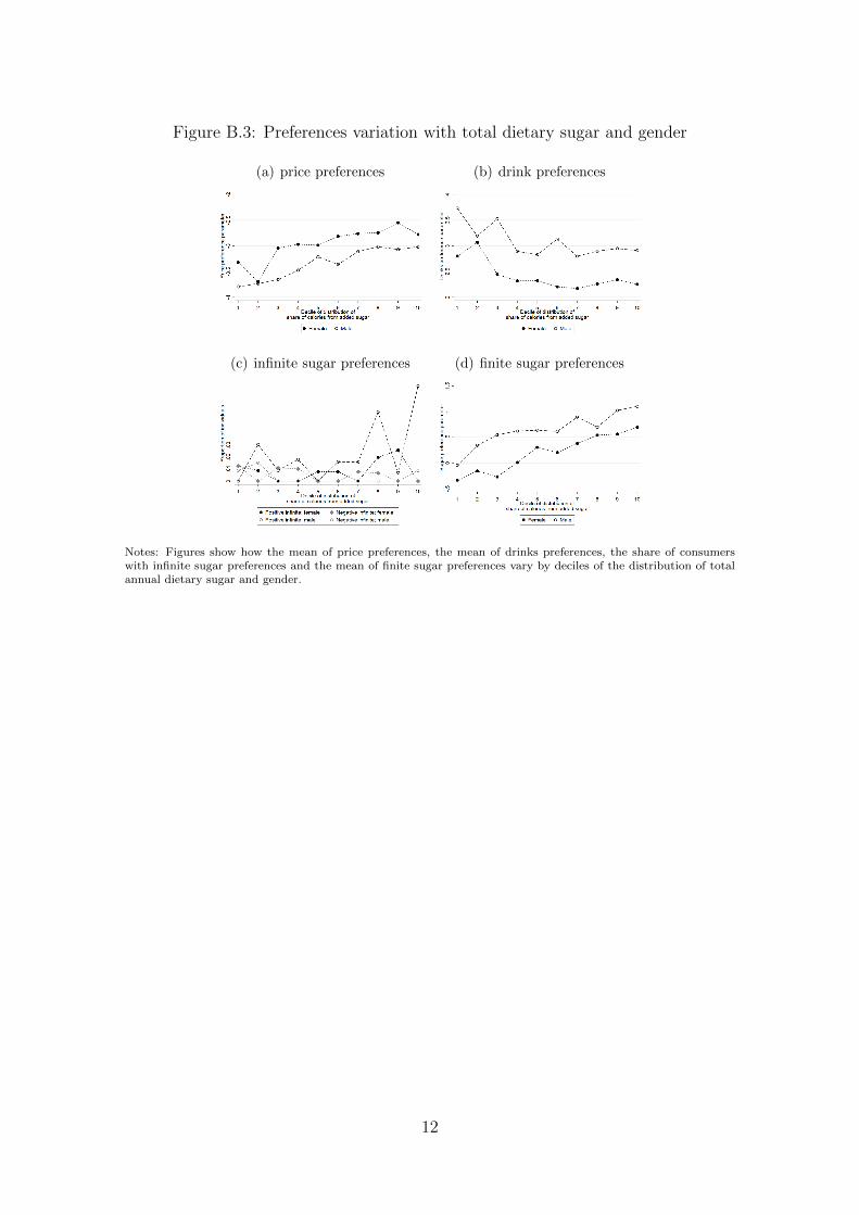
Figure B.3: Preferences variation with total dietary sugar and gender

(a) price preferences (b) drink preferences

(c) infinite sugar preferences (d) finite sugar preferences

Notes: Figures show how the mean of price preferences, the mean of drinks preferences, the share of consumerswith infinite sugar preferences and the mean of finite sugar preferences vary by deciles of the distribution of totalannual dietary sugar and gender.

12

Figure B.4: Preferences variation with age and socioeconomic status

(a) price preferences (b) drink preferences

(c) infinite sugar preferences (d) finite sugar preferences

Notes: Figures show how the mean of price preferences, the mean of drinks preferences, the share of consumers withinfinite sugar preferences and the mean of finite sugar preferences vary by age and socioeconomic status. “High”refers to those from a household whose head works in managerial or professional roles, “Low” refers to those froma household whose head works in manual work or relies on the state for their income.

13

Figure B.5: Preferences variation with total dietary sugar and socioeconomic status

(a) price preferences (b) drink preferences

(c) infinite sugar preferences (d) finite sugar preferences

Notes: Figures show how the mean of price preferences, the mean of drinks preferences, the share of consumerswith infinite sugar preferences and the mean of finite sugar preferences vary by deciles of the total dietary sugarand socioeconomic status. “High” refers to those from a household whose head works in managerial or professionalroles, “Low” refers to those from a household whose head works in manual work or relies on the state for theirincome.

B.1 Incidental parameters problem

Figures B.6, B.7 and B.8 show, for the price, drinks and sugar preference param-

eters, how the jackknife (θsplit) and the maximum likelihood estimates (θ) relate

to a) the number of choice occasions of individuals that are in the sample, b) age

and c) total dietary sugar. They show no systematic relationship in the mean of

(θsplit− θ) with any of these variables, with the dispersion of (θsplit− θ) falling in T .

Figures B.9 plot the distributions of price, drinks and sugar preference parameter

estimates for both the estimators θ and θsplit, showing there is little difference in

the distributions.

14

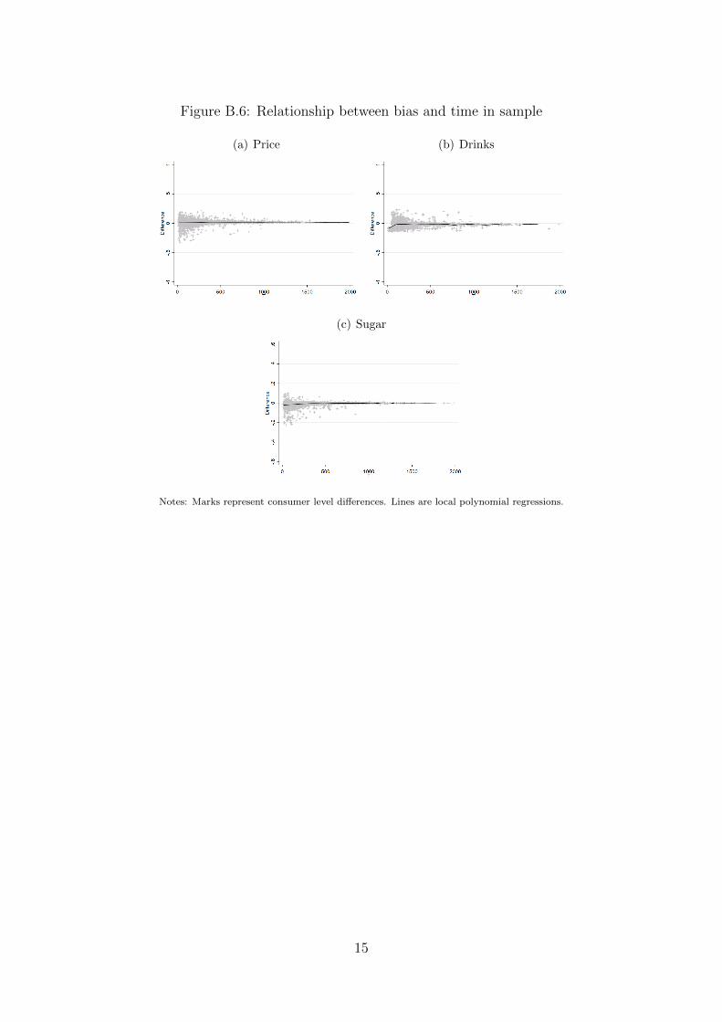
Figure B.6: Relationship between bias and time in sample

(a) Price (b) Drinks

(c) Sugar

Notes: Marks represent consumer level differences. Lines are local polynomial regressions.

15

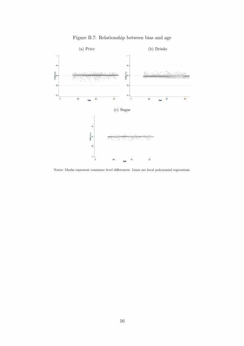
Figure B.7: Relationship between bias and age

(a) Price (b) Drinks

(c) Sugar

Notes: Marks represent consumer level differences. Lines are local polynomial regressions.

16

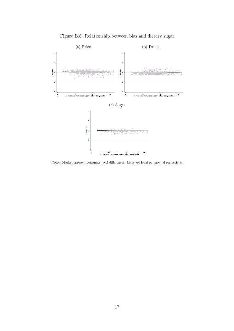
Figure B.8: Relationship between bias and dietary sugar

(a) Price (b) Drinks

(c) Sugar

Notes: Marks represent consumer level differences. Lines are local polynomial regressions.

17

Figure B.9: Preference parameter distribution

(a) Price (b) Drinks

(c) Sugar

Notes: Lines are kernel density estimates.

C Demand estimates in at-home segment

C.1 At-home data

We use information on the at-home behavior of 4,205 households over June 2009-

December 2014. Of these 3,059 households are drinks purchasers.1 Tables 2, 3 and

4 shows the panel dimension of the data, the products we model choice over in the

at-home segment and retailer types. This mirrors tables in Section I of the paper for

the on-the-go segment. In the at-home demand model a choice occasion is defined as

a week in which the household buys groceries and the outside option corresponds

to not buying any non-alcoholic drinks (exclusive for non-flavored milk). In the

estimation sample there are 653,063 choice occasions in total. Households choose

the outside option on 59% of choice occasions.

1Defined as buying at 15 non-alcoholic drinks over the 5 and a half year period of our data.

18

Table 2: Time series dimension of at-home estimation sample

Number of choice Individualsoccasions observed on-the-go

N %

<25 20 0.725-49 59 1.950-74 106 3.575-99 151 4.9100-249 1573 51.4250+ 1150 37.6

Total 3059 100.0

Notes: The table shows the number of choice occasions on which we observe household making at-home purchasechoices based on the 3,059 households in the at-home estimation sample. A choice occasion is a week in which thehousehold visits the grocery store.

19

Table 3: Products in at-home sample

Firm Brand Product % price

Soft drinksCocaCola 22.24

Coke 16.70Coca Cola Diet 330 0.15 0.57Coca Cola 330 0.21 0.57Coca Cola 500 0.74 1.01Coca Cola Diet 500 1.18 1.01Coca Cola multi can 2.50 3.43Coca Cola Diet multi can 4.05 3.37Coca Cola bottle 3.37 1.40Coca Cola Diet bottle 4.27 1.37Coca Cola multi bottle 0.14 5.27Coca Cola Diet multi bottle 0.09 5.73

Dr Pepper 1.60Dr Pepper 330 0.02 0.55Dr Pepper 500 0.23 1.00Dr Pepper multi can 0.27 2.46Dr Pepper Diet multi can 0.11 2.41Dr Pepper bottle 0.72 1.36Dr Pepper Diet bottle 0.26 1.31

Fanta 1.78Fanta 500 0.24 1.01Fanta multi can 0.23 2.33Fanta Diet multi can 0.25 2.53Fanta bottle 0.82 1.33Fanta Diet bottle 0.24 1.32

Cherry Coke 0.86Cherry Coke 330 0.02 0.52Cherry Coke Diet 500 0.10 1.03Cherry Coke 500 0.14 1.03Cherry Coke multi can 0.13 2.90Cherry Coke Diet multi can 0.12 2.84Cherry Coke bottle 0.22 1.34Cherry Coke Diet bottle 0.12 1.32

Oasis 0.38Oasis 500 0.38 1.01

Sprite 0.93Sprite 500 0.12 1.00Sprite multi can 0.11 2.37Sprite Diet multi can 0.16 2.38Sprite bottle 0.35 1.33Sprite Diet bottle 0.20 1.34

Pepsico 12.71Pepsi Diet 330 0.16 0.40Pepsi 330 0.07 0.40Pepsi 500 0.25 0.81Pepsi Diet 500 0.71 0.81Pepsi multi can 1.04 2.14Pepsi Diet multi can 3.06 2.17Pepsi bottle 2.00 1.09Pepsi Diet bottle 5.43 1.10

GSK 3.62Lucozade Energy 3.04

Lucozade Energy 380 0.21 0.76Lucozade Energy 500 0.32 1.03Lucozade Energy bottle 1.41 1.14Lucozade Energy multi bottle 1.11 3.05

Ribena 0.58Ribena 288 0.03 0.55Ribena 500 0.08 1.05Ribena multi 0.47 1.98

1.09Irn Bru 500 0.04 0.94Irn Bru Diet 500 0.04 0.94Irn Bru multi can 0.08 2.53Irn Bru Diet multi can 0.10 2.44Irn Bru bottle 0.44 1.19Irn Bru Diet bottle 0.39 1.1920

Table 3 cont.

Firm Brand Product % price

Composite soft drinksOther 2.23 1.23Other bg 2.71 1.05Other Diet bg 1.11 1.03Other multi 1.02 2.08Other Diet multi 0.35 1.87

Alternative drinksFruit juice 3.13 1.62Fruit juice 18.38 1.40Flavoured milk 3.32 0.79Flavoured milk 1.30 1.05Fruit water 0.04 0.76Fruit water 0.67 0.91Water 0.71 0.48Water 10.89 0.89

Notes: Market shares are based on transactions made by the 3,059 households in the at-home estimation samplebetween June 2009 and December 2014. Prices are the means across all choice occasions.

Table 4: Retailer types in at-home sample

N %

Retailer types

Big four Asda 123,576 18.9Morrisons 86,949 13.3Sainsbury’s 85,486 13.1Tesco 215,619 33.0

Discounters 44,207 6.8Other 97,226 14.9

Total 653,063 100.0

Notes: The table shows the number and share of purchases made by 3,059 households in the at-home estimationsample in each retailer type between June 2009 and December 2014.

C.2 At-home demand estimates

In Table 5 we summarize estimates of the household specific preference parameters

governing at-home demand. In Figure C.1 we report estimates of the demographic

specific preference parameters.

21

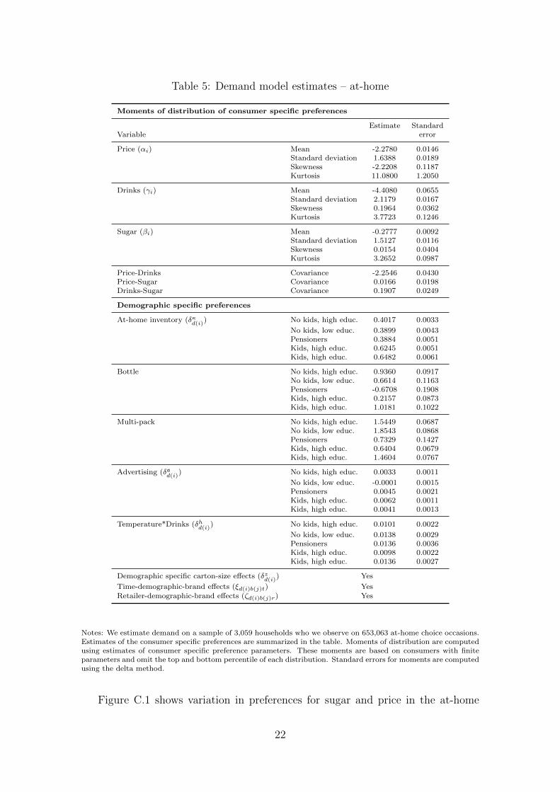
Table 5: Demand model estimates – at-home

Moments of distribution of consumer specific preferences

Estimate StandardVariable error

Price (αi) Mean -2.2780 0.0146Standard deviation 1.6388 0.0189Skewness -2.2208 0.1187Kurtosis 11.0800 1.2050

Drinks (γi) Mean -4.4080 0.0655Standard deviation 2.1179 0.0167Skewness 0.1964 0.0362Kurtosis 3.7723 0.1246

Sugar (βi) Mean -0.2777 0.0092Standard deviation 1.5127 0.0116Skewness 0.0154 0.0404Kurtosis 3.2652 0.0987

Price-Drinks Covariance -2.2546 0.0430Price-Sugar Covariance 0.0166 0.0198Drinks-Sugar Covariance 0.1907 0.0249

Demographic specific preferences

At-home inventory (δκd(i)

) No kids, high educ. 0.4017 0.0033

No kids, low educ. 0.3899 0.0043Pensioners 0.3884 0.0051Kids, high educ. 0.6245 0.0051Kids, high educ. 0.6482 0.0061

Bottle No kids, high educ. 0.9360 0.0917No kids, low educ. 0.6614 0.1163Pensioners -0.6708 0.1908Kids, high educ. 0.2157 0.0873Kids, high educ. 1.0181 0.1022

Multi-pack No kids, high educ. 1.5449 0.0687No kids, low educ. 1.8543 0.0868Pensioners 0.7329 0.1427Kids, high educ. 0.6404 0.0679Kids, high educ. 1.4604 0.0767

Advertising (δad(i)

) No kids, high educ. 0.0033 0.0011

No kids, low educ. -0.0001 0.0015Pensioners 0.0045 0.0021Kids, high educ. 0.0062 0.0011Kids, high educ. 0.0041 0.0013

Temperature*Drinks (δhd(i)

) No kids, high educ. 0.0101 0.0022

No kids, low educ. 0.0138 0.0029Pensioners 0.0136 0.0036Kids, high educ. 0.0098 0.0022Kids, high educ. 0.0136 0.0027

Demographic specific carton-size effects (δzd(i)

) Yes

Time-demographic-brand effects (ξd(i)b(j)t) YesRetailer-demographic-brand effects (ζd(i)b(j)r) Yes

Notes: We estimate demand on a sample of 3,059 households who we observe on 653,063 at-home choice occasions.Estimates of the consumer specific preferences are summarized in the table. Moments of distribution are computedusing estimates of consumer specific preference parameters. These moments are based on consumers with finiteparameters and omit the top and bottom percentile of each distribution. Standard errors for moments are computedusing the delta method.

Figure C.1 shows variation in preferences for sugar and price in the at-home

22

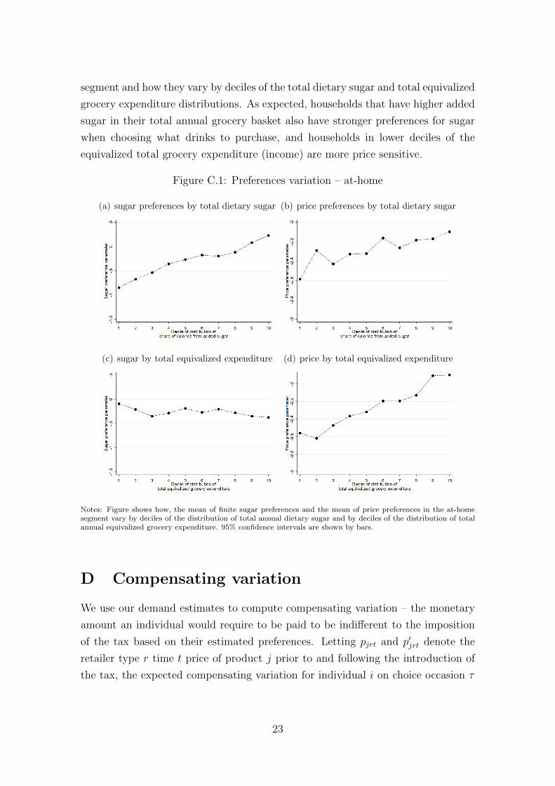
segment and how they vary by deciles of the total dietary sugar and total equivalized

grocery expenditure distributions. As expected, households that have higher added

sugar in their total annual grocery basket also have stronger preferences for sugar

when choosing what drinks to purchase, and households in lower deciles of the

equivalized total grocery expenditure (income) are more price sensitive.

Figure C.1: Preferences variation – at-home

(a) sugar preferences by total dietary sugar (b) price preferences by total dietary sugar

(c) sugar by total equivalized expenditure (d) price by total equivalized expenditure

Notes: Figure shows how, the mean of finite sugar preferences and the mean of price preferences in the at-homesegment vary by deciles of the distribution of total annual dietary sugar and by deciles of the distribution of totalannual equivalized grocery expenditure. 95% confidence intervals are shown by bars.

D Compensating variation

We use our demand estimates to compute compensating variation – the monetary

amount an individual would require to be paid to be indifferent to the imposition

of the tax based on their estimated preferences. Letting pjrt and p′jrt denote the

retailer type r time t price of product j prior to and following the introduction of

the tax, the expected compensating variation for individual i on choice occasion τ

23

is given by (Small and Rosen (1981)):

cviτ =1

αi

ln

∑k∈Ωi∩Ωr(τ)

exp(vikr(τ)t(τ) + ηikr(τ)t(τ) − αi(pkr(τ)t(τ) − p′kr(τ)t(τ))) + 10∈Ωi exp(βi)

−ln

∑k∈Ωi∩Ωr(τ)

exp(vikr(τ)t(τ) + ηikr(τ)t(τ)) + 10∈Ωi exp(βi)

where vijr(τ)t(τ) and ηijr(τ)t(τ) are defined in Section II.A .2 Summing cviτ over an

individual’s choice occasions in the year gives their annual compensating variation.

E Equilibrium tax pass-through

In Section IV.C we show that our results on the targeting of a soda tax are similar

under the assumption of 100% pass-through and under estimates of equilibrium

tax pass-through. Here we provide further details of our model of equilibrium tax

pass-through.

We model tax pass-through by assuming that drinks manufacturers compete

by simultaneously setting prices in a Nash-Bertrand game. We consider a mature

market with a stable set of products, and we therefore abstract from entry and exit

of firms and products from the market. We use our demand estimates for the on-

the-go market, demand estimates for the at-home market (described in Appendix

C) and an equilibrium pricing condition to infer firms’ marginal costs (see Berry

(1994) or Nevo (2001)) in order to then simulate the effect of a tax on consumer

prices.

Let f = 1, . . . , F index manufacturers and Ff denote the set of products

owned by firm f . We assume that prices are set by manufacturers and abstract from

modeling manufacturer-retailer relationships. Such an outcome can be achieved by

vertical contracting (Villas-boas (2007), Bonnet and Dubois (2010)).3 Bonnet and

Dubois (2010) show that in the French grocery market price equilibria correspond to

the case where manufacturers and retailers do use non-linear contracts in the form

of two part tariffs. Testing for the form of vertical contracting in UK manufacturer-

retailer relations is an interesting question that we leave for future research.

We index markets by m. Markets vary over time and across retailer type. In

particular a market is defined as a year-retailer pair. We denote the size of the

2Note, that vijr(τ)t(τ) is defined such that it includes the effect of price prior to the introductionof the tax.

3Non-linear contracts with side transfers between manufacturers and retailers allow them toreallocate profits and avoid the double marginalization problem.

24

on-the-go segment in market m by M outm and the size of the at-home segment by

M inm and we denote the set of individual-choice occasions in the on-the-go and at-

home segments of market m as Moutm and Min

m . Aggregating across consumer level

purchase probabilities we obtain the market level demand function for product j:

qjm(pm) = M outm

∑(i,τ)∈Mout

m

Piτ (j)︸ ︷︷ ︸≡qoutjm (pm)

+M inm

∑(i,τ)∈Min

m

Piτ (j)︸ ︷︷ ︸≡qinjm(pm)

for each product j and where Piτ (j) follows equation (2).

If product j is available only in the at-home segment (e.g. if it is a large multi

portion product), then Piτ (j) = 0 for all (i, τ) ∈Moutm , and if it is only available in

the on-the-go segment then Piτ (j) = 0 for all (i, τ) ∈ Minm . However, for products

available in both on-the-go and at-home segments the market demand curve depends

on purchase probabilities (and hence preferences) in both segment.

Firm f ’s (variable) profits in market m are given by:

Πfm =∑j∈Ff

(pjm − cjm)qjm(pm) (1)

and the firm’s price first order conditions are:

qjm(pm) +∑k∈Ff

(pkm − ckm)∂qkm(pm)

∂pjm= 0 ∀j ∈ Ff . (2)

Under the assumption that observed market prices are an equilibrium outcome

of the Nash-Bertrand game played by firms, and given our estimates of the demand

function, we can invert the first order conditions to infer marginal costs cjm. The

introduction of a tax creates a wedge between post-tax prices, p, and pre-tax prices,

which we denote p. The volumetric tax, π, on sugary soft drinks (denoted by the

set Ωws) implies pre-tax and post-tax prices are related by:

pjm =

pjm + πlj

pjm

∀j ∈ Ωws

∀j /∈ Ωws

where lj is the volume of product j.

In the counterfactual equilibrium, prices satisfy the conditions:

qjm(pm) +∑k∈Ff

(pkm − ckm)∂qkm(pm)

∂pjm= 0 ∀j ∈ Ff (3)

for all firms f . We solve for the new equilibrium prices as the vector that satisfies

25

the set of first order conditions (equation (3)) when π = 0.25.4 Tax pass-through

describes how much of the tax is shifted through to post-tax prices, for products

j ∈ Ωws, we measure this as the difference in the post-tax and pre-tax equilibrium

consumer price over the amount of tax levied, πlj.5

References

Berkson, J. 1950. “Are There Two Regressions?” Journal of the American Sta-

tistical Association, 45(250): 164–180.

Berry, Steven T. 1994. “Estimating Discrete-Choice Models of Product Differen-

tiation.” RAND Journal of Economics, 25: 242–262.

Blundell, Richard, Joel Horowtiz, and Matthias Parey. 2019. “Estimation

of a Nonseparable Heterogenous Demand Function with Shape Restrictions and

Berkson Errors.” CWP67/18.

Bonnet, Celine, and Pierre Dubois. 2010. “Inference on Vertical Contracts

between Manufacturers and Retailers Allowing for Nonlinear Pricing and Resale

Price Maintenance.” RAND Journal of Economics, 41(1): 139–164.

Nevo, Aviv. 2001. “Measuring Market Power in the Ready-to-Eat Cereal Indus-

try.” Econometrica, 69(2): 307–342.

Schennach, Susanne. 2013. “Regressions with Berkson Errors in Covariates – A

Nonparametric Approach.” The Annals of Statistics, 41: 1642–1668.

Small, Kenneth A, and Harvey S Rosen. 1981. “Applied Welfare Economics

with Discrete Choice Models.” Econometrica, 49(1): 105–130.

Villas-boas, Sofia Berto. 2007. “Vertical Relationships between Manufactur-

ers and Retailers: Inference with Limited Data.” Review of Economic Studies,

74(2): 625–652.

4We solve for a new equilibrium price for each of the products belonging to the main soft drinksbrands; we assume there is no change in the producer price (and therefore 100% pass-through)of the composite other soft drinks brand (which aggregates together many very small soft drinksbrands). We also assume no pricing response for the set of outside products.

5We solve for separate price equilibrium in each of the 11 retailers and for a representativemonth in each year, giving us 66 price equilibria.

26