Online 3D CoM Trajectory Generation for Multi-Contact LocomotionSynchronizing Contact

Mitsuharu Morisawa1,∗, Rafael Cisneros1, Mehdi Benallegue1,Iori Kumagai1, Adrien Escande2, Fumio Kanehiro1

Abstract— This paper proposes a fast computation methodfor 3D multi-contact locomotion. The contributions of this paperare (a) the derivation of the prospect centroidal dynamics byintroducing a force distribution ratio, where the centroidaldynamics in multi-contact can be represented with a formu-lation similar to the inverted pendulum’s one, and (b) thedevelopment of a fast computation method for generating a3D center of mass (CoM) trajectory. The proposed methodallows to generate a trajectory sequentially and to changethe locomotion parameters at any time even under variableCoM height. Then, the contact timing of each end-effector canbe adjusted to synchronize with the actual contact with theenvironment by shortening or extending the desired durationof the support phase. This can be used to improve the robustnessof the locomotion. In this paper, we deal with a multi-contactlocomotion which can be fully received a vertical reaction forcefrom the environment and the validity of the proposed method isconfirmed by several numerical results: the CoM motion whilechanging the contact timing and a multi-contact locomotionconsidering a transition between biped and quadruped walkingin a dynamics simulator.

I. INTRODUCTION

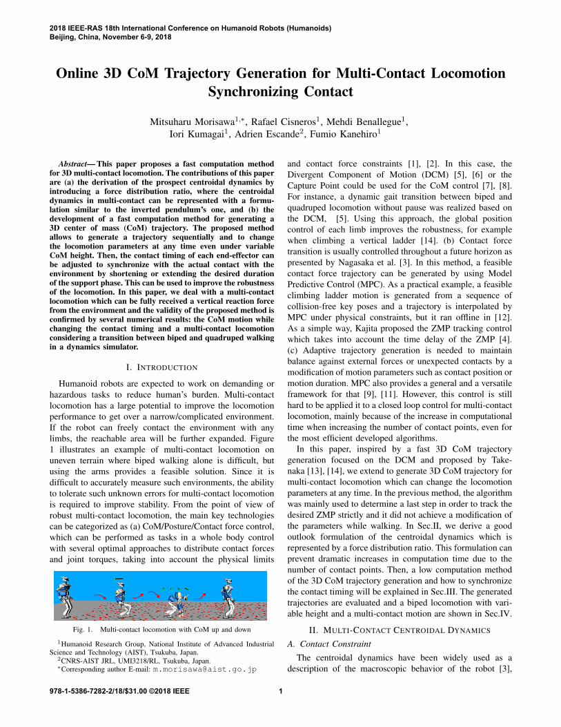
Humanoid robots are expected to work on demanding orhazardous tasks to reduce human’s burden. Multi-contactlocomotion has a large potential to improve the locomotionperformance to get over a narrow/complicated environment.If the robot can freely contact the environment with anylimbs, the reachable area will be further expanded. Figure1 illustrates an example of multi-contact locomotion onuneven terrain where biped walking alone is difficult, butusing the arms provides a feasible solution. Since it isdifficult to accurately measure such environments, the abilityto tolerate such unknown errors for multi-contact locomotionis required to improve stability. From the point of view ofrobust multi-contact locomotion, the main key technologiescan be categorized as (a) CoM/Posture/Contact force control,which can be performed as tasks in a whole body controlwith several optimal approaches to distribute contact forcesand joint torques, taking into account the physical limits

Fig. 1. Multi-contact locomotion with CoM up and down

1Humanoid Research Group, National Institute of Advanced IndustrialScience and Technology (AIST), Tsukuba, Japan.

2CNRS-AIST JRL, UMI3218/RL, Tsukuba, Japan.∗Corresponding author E-mail: m.morisawa@aist.go.jp

and contact force constraints [1], [2]. In this case, theDivergent Component of Motion (DCM) [5], [6] or theCapture Point could be used for the CoM control [7], [8].For instance, a dynamic gait transition between biped andquadruped locomotion without pause was realized based onthe DCM, [5]. Using this approach, the global positioncontrol of each limb improves the robustness, for examplewhen climbing a vertical ladder [14]. (b) Contact forcetransition is usually controlled throughout a future horizon aspresented by Nagasaka et al. [3]. In this method, a feasiblecontact force trajectory can be generated by using ModelPredictive Control (MPC). As a practical example, a feasibleclimbing ladder motion is generated from a sequence ofcollision-free key poses and a trajectory is interpolated byMPC under physical constraints, but it ran offline in [12].As a simple way, Kajita proposed the ZMP tracking controlwhich takes into account the time delay of the ZMP [4].(c) Adaptive trajectory generation is needed to maintainbalance against external forces or unexpected contacts by amodification of motion parameters such as contact position ormotion duration. MPC also provides a general and a versatileframework for that [9], [11]. However, this control is stillhard to be applied it to a closed loop control for multi-contactlocomotion, mainly because of the increase in computationaltime when increasing the number of contact points, even forthe most efficient developed algorithms.

In this paper, inspired by a fast 3D CoM trajectorygeneration focused on the DCM and proposed by Take-naka [13], [14], we extend to generate 3D CoM trajectory formulti-contact locomotion which can change the locomotionparameters at any time. In the previous method, the algorithmwas mainly used to determine a last step in order to track thedesired ZMP strictly and it did not achieve a modification ofthe parameters while walking. In Sec.II, we derive a goodoutlook formulation of the centroidal dynamics which isrepresented by a force distribution ratio. This formulation canprevent dramatic increases in computation time due to thenumber of contact points. Then, a low computation methodof the 3D CoM trajectory generation and how to synchronizethe contact timing will be explained in Sec.III. The generatedtrajectories are evaluated and a biped locomotion with vari-able height and a multi-contact motion are shown in Sec.IV.

II. MULTI-CONTACT CENTROIDAL DYNAMICS

A. Contact Constraint

The centroidal dynamics have been widely used as adescription of the macroscopic behavior of the robot [3],

2018 IEEE-RAS 18th International Conference on Humanoid Robots (Humanoids)Beijing, China, November 6-9, 2018

978-1-5386-7282-2/18/$31.00 ©2018 IEEE 1

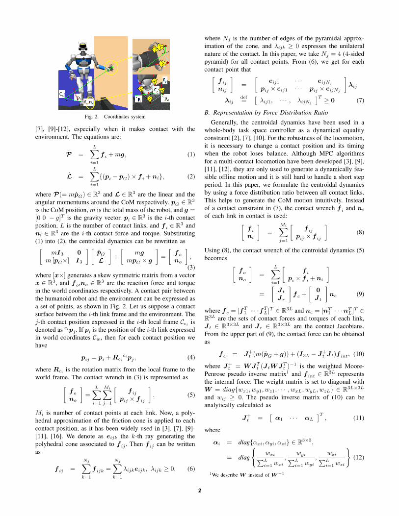
Fig. 2. Coordinates system

[7], [9]-[12], especially when it makes contact with theenvironment. The equations are:

P =

L∑i=1

f i +mg, (1)

L =L∑

i=1

{(pi − pG)× f i + ni}, (2)

where P(= mpG) ∈ R3 and L ∈ R3 are the linear and theangular momentums around the CoM respectively. pG ∈ R3

is the CoM position, m is the total mass of the robot, and g =[0 0 − g]T is the gravity vector. pi ∈ R3 is the i-th contactposition, L is the number of contact links, and f i ∈ R3 andni ∈ R3 are the i-th contact force and torque. Substituting(1) into (2), the centroidal dynamics can be rewritten as[

mI3 0m [pG×] I3

] [pG

L

]+

[mg

mpG × g

]=

[fo

no

],

(3)where [x×] generates a skew symmetric matrix from a vectorx ∈ R3, and fo,no ∈ R3 are the reaction force and torquein the world coordinates respectively. A contact pair betweenthe humanoid robot and the environment can be expressed asa set of points, as shown in Fig. 2. Let us suppose a contactsurface between the i-th link frame and the environment. Thej-th contact position expressed in the i-th local frame Cci isdenoted as cipj . If pi is the position of the i-th link expressedin world coordinates Cw, then for each contact position wehave

pij = pi +Rcicipj , (4)

where Rci is the rotation matrix from the local frame to theworld frame. The contact wrench in (3) is represented as[

fo

no

]=

L∑i=1

Mi∑j=1

[f ij

pij × f ij

]. (5)

Mi is number of contact points at each link. Now, a poly-hedral approximation of the friction cone is applied to eachcontact position, as it has been widely used in [3], [7], [9]-[11], [16]. We denote as eijk the k-th ray generating thepolyhedral cone associated to f ij . Then f ij can be writtenas

f ij =

Nj∑k=1

f ijk =

Nj∑k=1

λijkeijk, λijk ≥ 0, (6)

where Nj is the number of edges of the pyramidal approx-imation of the cone, and λijk ≥ 0 expresses the unilateralnature of the contact. In this paper, we take Nj = 4 (4-sidedpyramid) for all contact points. From (6), we get for eachcontact point that[

f ij

nij

]=

[eij1 · · · eijNj

pij × eij1 · · · pij × eijNj

]λij

λijdef=

[λij1, · · · , λijNj

]T ≥ 0 (7)

B. Representation by Force Distribution Ratio

Generally, the centroidal dynamics have been used in awhole-body task space controller as a dynamical equalityconstraint [2], [7], [10]. For the robustness of the locomotion,it is necessary to change a contact position and its timingwhen the robot loses balance. Although MPC algorithmsfor a multi-contact locomotion have been developed [3], [9],[11], [12], they are only used to generate a dynamically fea-sible offline motion and it is still hard to handle a short stepperiod. In this paper, we formulate the centroidal dynamicsby using a force distribution ratio between all contact links.This helps to generate the CoM motion intuitively. Insteadof a contact constraint in (7), the contact wrench f i and ni

of each link in contact is used:[f i

ni

]=

Mi∑j=1

[f ij

pij × f ij

](8)

Using (8), the contact wrench of the centroidal dynamics (5)becomes [

fo

no

]=

L∑i=1

[f i

pi × f i + ni

]=

[J t

Jr

]f c +

[0J t

]nc (9)

where f c = [fT1 · · ·fT

L]T ∈ R3L and nc = [nT

1 · · ·nTL]

T ∈R3L are the sets of contact forces and torques of each link,J t ∈ R3×3L and Jr ∈ R3×3L are the contact Jacobians.From the upper part of (9), the contact force can be obtainedas

f c = J+t (m(pG + g)) + (I3L − J+

t J t)f int, (10)

where J+t = WJT

t (J tWJTt )

−1 is the weighted Moore-Penrose pseudo inverse matrix1 and f int ∈ R3L representsthe internal force. The weight matrix is set to diagonal withW = diag{wx1, wy1, wz1, · · · , wxL, wyL, wzL} ∈ R3L×3L

and wij ≥ 0. The pseudo inverse matrix of (10) can beanalytically calculated as

J+t =

[α1 · · · αL

]T, (11)

where

αi = diag{αxi, αyi, αzi} ∈ R3×3,

= diag

{wxi∑Li=1 wxi

,wyi∑Li=1 wyi

,wzi∑Li=1 wzi

}(12)

1We describe W instead of W−1

2

From (12), the sum of weight in each axis obviously becomesL∑

i=1

αxi =L∑

i=1

αyi =L∑

i=1

αzi = 1. (13)

Let us denote α◦i as a force distribution ratio for theCoM motion. We represent a force distribution by a timepolynomial function to realize an appropriate force transition.From (3), (9) and (10), the angular momentum rate of thecentroidal dynamics can be expressed as

([pG×]−L∑

i=1

[pi×]αi) pG

= − ([pG×]−L∑

i=1

[pi×]αi) g − σ

m, (14)

where

σ = −L+ Jr(I3L − J+t J t)f int + nc (15)

In case of non flat plane, the internal force affects the inertialCoM motion through the nullspace projection matrix in thesecond term of the right side of (10). By extracting thehorizontal CoM motion, (14) can be represented as

xG =g + zG

zG −∑L

i=1 αxipzi(xG −

L∑i=1

αzipxi +σy

m(g + zG)

), (16)

yG =g + zG

zG −∑L

i=1 αyipzi(yG −

L∑i=1

αzipyi −σx

m(g + zG)

),

where∑L

i=1 αxipzi and∑L

i=1 αyipzi encode the virtualheight via zh = zG−

∑Li=1 α◦ipzi(◦ = x, y), i.e. the denomi-

nator mentioned above is the pendulum height. When the vir-tual height is higher than the CoM height, the CoM behavesas a non-inverted pendulum.

∑Li=1 αzipxi and

∑Li=1 αzipyi

consist of the representative contact point and the other termwhich is the derivative of the angular momentum and relatedto the contact force on a non-flat surface. When the contactpositions allow force closure, the CoM can be moved in anydirection [16].

III. ONLINE COM TRAJECTORY GENERATION FORMULTI-CONTACT

As a way to improve the adaptability of locomotion, theCoM trajectory can be generated in synchronization withthe contacts with the environment. When the desired contactposition and timing are preplanned, it is necessary to generatemulti-contact locomotion sequentially so that the timing orcontact position can be immediately changed. In this section,we propose a very fast computation method of the CoMtrajectory under this dynamics. From the basic concept in[8], [19], the trajectory generation is composed of 2 terms:a long and a short term trajectory.

A. Long term trajectory of the CoM

In a similar way to [5], the discretized system of thecentroidal dynamics in the sagittal plane of (16) with asampling period ∆T can be obtained as

xk+1 = Akxk +Bkuk, (17)

where,

xk =

[xG,k

xG,k

], uk =

L∑i=1

αzi,kpxi,k − σy,k

m(g + zG,k),

Ak =

[cosh(ωk∆T ) sinh(ωk∆T )

ωk

ωk sinh(ωk∆T ) cosh(ωk∆T )

],

Bk =

[1− cosh(ωk∆T )−ωk sinh(ωk∆T )

],

ωk =

√g + zG,k

zG,k −∑L

i=1 αxi,kpzi,k. (18)

where uk is equivalent to the ZMP2. This equation becomes aLinear Time-Varying System (LTVS) under a variable heightof the CoM, the angular momentum rate, a varying forcedistribution ratio, and an internal force. The CoM motion inthe frontal plane can be also discussed as the same way as inthe sagittal plane (18). When the future sequence of a contactposition, a force transition and also the angular momentumrate are preplanned, the future input of uk will be given. TheCoM state xF after the F -th future step is

xF = Φ(F, 0)x0 +F−1∑i=0

Φ(F, i+ 1)Biui (19)

where,

Φ(k, j) =

{Ak−1Ak−2 · · ·Aj if k > jI2 otherwise (k = j = F )

Generally in order to generate a smooth trajectory sequen-tially, the boundary condition as the CoM position andvelocity also the ZMP position should be satisfied. Further-more, an input u as a representative center of pressure isalso restricted under the physical contact condition. Thisinput causes a variation to accelerate/decelerate the CoMwhen starting/stopping the locomotion, or when changing it.Therefore the computational cost to find an optimal input uunder these constraints becomes high.

In the case of MPC, the trajectory can be generated as a QPproblem which is solved to find a set of inputs u0 · · ·uF suchthat the generated trajectory can track the desired one. Inthe calculation process for LTVS, one has to solve a systemof linear equations with a number of variables proportionalto the length of preview window divided by the samplingperiod. In this paper, we introduce a simple boundary con-dition to calculate the long term trajectory online. In orderto reduce the variation of the input, we calculate a trajectoryfrom past contact parameters. Instead of the preview windowgoing from the current step 0 to the future step F in (19), we

2More exactly, this is named as the Centroidal Momentum Pivod (CMP)with Lx = 0, and Ly = 0 [17]

3

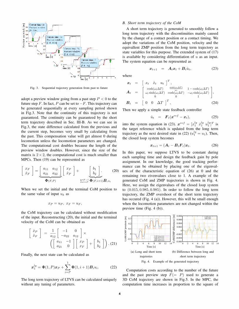
Fig. 3. Sequential trajectory generation from past to future

adopt a preview window going from a past step P < 0 to thefuture step F . In fact, P can be set to −F . This trajectory canbe generated sequentially at every sampling period shownin Fig.3. Note that the continuity of this trajectory is notguaranteed. The continuity can be guaranteed by the shortterm trajectory described in Sec. III-B. As we can see inFig.3, the state difference calculated from the previous andthe current step, becomes very small by calculating fromthe past. This compensation value will get almost 0 duringlocomotion unless the locomotion parameters are changed.The computational cost doubles because the length of thepreview window doubles. However, since the size of thematrix is 2× 2, the computational cost is much smaller thanMPCs. Then (19) can be represented as[

xF

xF

]=

[a11 a12a21 a22

]︸ ︷︷ ︸

Φ(F,P )

[xP

xP

]+

[b1b2

].︸ ︷︷ ︸∑F−1

i=P Φ(F,i+1)Biui

(20)

When we set the initial and the terminal CoM position tothe same value of input uk as

xP = uP , xF = uF ,

the CoM trajectory can be calculated without modificationof the input. Reconstructing (20), the initial and the terminalvelocity of the CoM can be obtained as[

xP

xF

]=

1

a12

[−1 0−a22 a12

]×([

a11 −1a21 0

] [xP

xF

]+

[b1b2

]). (21)

Finally, the next state can be calculated as

xlg1 = Φ(1, P )xP +

1∑i=P

Φ(1, i+ 1)Biui. (22)

The long term trajectory of LTVS can be calculated uniquelywithout any tuning of parameters.

B. Short term trajectory of the CoM

A short term trajectory is generated to smoothly follow along term trajectory with the discontinuities mainly causedby the change of a contact position or a contact timing. Weadopt the variations of the CoM position, velocity and theequivallent ZMP position from the long term trajectory asstate variables for this purpose. The extended system of (17)is available by considering differentiation of u as an input.The system equation can be represented as

xt+1 = Atxt +Btut, (23)

where

xt =[xt xt ut

]T,

At =

cosh(ωt∆T ) sinh(ωt∆T )ωt

1− cosh(ωt∆T )

ωt sinh(ωt∆T ) cosh(ωt∆T ) −ωt sinh(ωt∆T )0 0 1

,Bt =

[0 0 ∆T

]T, (24)

Then we apply a simple state feedback controller

ut = F t(xref − xt), (25)

into the system equation in (23). xref = [xlg1 xlg

1 ulg1 ]T is

the target reference which is updated from the long termtrajectory as the next desired state in (22) (ulg

1 = u1). Then,the closed loop system becomes

xt+1 = (At −BtF t)xt. (26)

In this paper, we suppose LTVS to be constant duringeach sampling time and design the feedback gain by poleassignment. In our knowledge, the good tracking perfor-mance can be obtained by placing one of the eigenval-ues of the characteristic equation of (26) at 0 and theremaining two eivenvalues close to 1. A example of thegenerated CoM and ZMP trajectories is shown in Fig. 4.Here, we assign the eigenvalues of the closed loop systemto (0.015, 0.985, 0.985). In order to follow the long termtrajectory, the ZMP overshoot of the short term trajectoryhas occured (Fig. 4 (a)). However, this will be small enoughwhen the locomotion parameters are not changed within thepreview time (Fig. 4 (b)).

-0.1

0

0.1

0.2

0.3

0 2 4 6 8 10 12 14

Co

M/Z

MP

posi

tio

n [

m]

Time [s]

CoM (long term)CoM (short term)ZMP (long term)ZMP (short term)

(a) Long and short termtrajetories

-0.006

-0.004

-0.002

0

0.002

0.004

0.006

0.008

0 2 4 6 8 10 12 14

Co

M/Z

MP

dif

fere

nces

[m]

Time [s]

CoM (diff)ZMP (diff)

(b) Difference between long andshort term trajectory

Fig. 4. Example of the generated trajectory

Computation costs according to the number of the futureand the past preview step F (= P ) used to generate a3D CoM trajectory are shown in Fig.5. In the MPC, thecomputation time increases in proportion to the square of

4

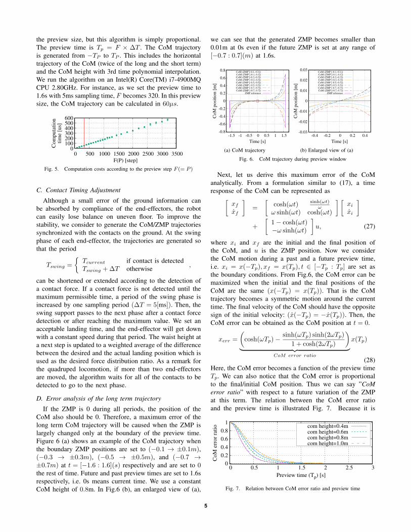
the preview size, but this algorithm is simply proportional.The preview time is Tp = F × ∆T . The CoM trajectoryis generated from −TP to TP . This includes the horizontaltrajectory of the CoM (twice of the long and the short term)and the CoM height with 3rd time polynomial interpolation.We run the algorithm on an Intel(R) Core(TM) i7-4900MQCPU 2.80GHz. For instance, as we set the preview time to1.6s with 5ms sampling time, F becomes 320. In this previewsize, the CoM trajectory can be calculated in 60µs.

0 100 200 300 400 500 600

0 500 1000 1500 2000 2500 3000 3500

Co

mp

uta

tio

nti

me

[us]

F(P) [step]

Fig. 5. Computation costs according to the preview step F (= P )

C. Contact Timing Adjustment

Although a small error of the ground information canbe absorbed by compliance of the end-effectors, the robotcan easily lose balance on uneven floor. To improve thestability, we consider to generate the CoM/ZMP trajectoriessynchronized with the contacts on the ground. At the swingphase of each end-effector, the trajectories are generated sothat the period

Tswing =

{Tcurrent if contact is detectedTswing +∆T otherwise ,

can be shortened or extended according to the detection ofa contact force. If a contact force is not detected until themaximum permissible time, a period of the swing phase isincreased by one sampling period (∆T = 5[ms]). Then, theswing support passes to the next phase after a contact forcedetection or after reaching the maximum value. We set anacceptable landing time, and the end-effector will get downwith a constant speed during that period. The waist height ata next step is updated to a weighted average of the differencebetween the desired and the actual landing position which isused as the desired force distribution ratio. As a remark forthe quadruped locomotion, if more than two end-effectorsare moved, the algorithm waits for all of the contacts to bedetected to go to the next phase.

D. Error analysis of the long term trajectory

If the ZMP is 0 during all periods, the position of theCoM also should be 0. Therefore, a maximum error of thelong term CoM trajectory will be caused when the ZMP islargely changed only at the boundary of the preview time.Figure 6 (a) shows an example of the CoM trajectory whenthe boundary ZMP positions are set to (−0.1 → ±0.1m),(−0.3 → ±0.3m), (−0.5 → ±0.5m), and (−0.7 →±0.7m) at t = [−1.6 : 1.6](s) respectively and are set to 0the rest of time. Future and past preview times are set to 1.6srespectively, i.e. 0s means current time. We use a constantCoM height of 0.8m. In Fig.6 (b), an enlarged view of (a),

we can see that the generated ZMP becomes smaller than0.01m at 0s even if the future ZMP is set at any range of[−0.7 : 0.7](m) at 1.6s.

-0.8

-0.6

-0.4

-0.2

0

0.2

0.4

0.6

0.8

-1.5 -1 -0.5 0 0.5 1 1.5

Co

M p

osi

tion [

m]

Time [s]

CoM (ZMP [-0.1,-0.1])CoM (ZMP [-0.1, 0.1])CoM (ZMP [-0.3,-0.3])CoM (ZMP [-0.3, 0.3])CoM (ZMP [-0.5,-0.5])CoM (ZMP [-0.5, 0.5])CoM (ZMP [-0.7,-0.7])CoM (ZMP [-0.7, 0.7])

ZMP reference

(a) CoM trajectory

-0.03

-0.02

-0.01

0

0.01

0.02

0.03

-0.4 -0.2 0 0.2 0.4

Co

M p

osi

tion [

m]

Time [s]

CoM (ZMP [-0.1,-0.1])CoM (ZMP [-0.1, 0.1])CoM (ZMP [-0.3,-0.3])CoM (ZMP [-0.3, 0.3])CoM (ZMP [-0.5,-0.5])CoM (ZMP [-0.5, 0.5])CoM (ZMP [-0.7,-0.7])CoM (ZMP [-0.7, 0.7])

ZMP reference

(b) Enlarged view of (a)

Fig. 6. CoM trajectory during preview window

Next, let us derive this maximum error of the CoManalytically. From a formulation similar to (17), a timeresponse of the CoM can be represented as[

xf

xf

]=

[cosh(ωt) sinh(ωt)

ωω sinh(ωt) cosh(ωt)

] [xi

xi

]+

[1− cosh(ωt)−ω sinh(ωt)

]u, (27)

where xi and xf are the initial and the final position ofthe CoM, and u is the ZMP position. Now we considerthe CoM motion during a past and a future preview time,i.e. xi = x(−Tp), xf = x(Tp), t ∈ [−Tp : Tp] are set asthe boundary conditions. From Fig.6, the CoM error can bemaximized when the initial and the final positions of theCoM are the same (x(−Tp) = x(Tp)). That is the CoMtrajectory becomes a symmetric motion around the currenttime. The final velocity of the CoM should have the oppositesign of the initial velocity: (x(−Tp) = −x(Tp)). Then, theCoM error can be obtained as the CoM position at t = 0.

xerr =

(cosh(ωTp)−

sinh(ωTp) sinh(2ωTp)

1 + cosh(2ωTp)

)︸ ︷︷ ︸

CoM error ratio

x(Tp)

(28)Here, the CoM error becomes a function of the preview timeTp. We can also notice that the CoM error is proportionalto the final/initial CoM position. Thus we can say ”CoMerror ratio” with respect to a future variation of the ZMPat this term. The relation between the CoM error ratioand the preview time is illustrated Fig. 7. Because it is

0

0.2

0.4

0.6

0.8

1

0 0.5 1 1.5 2 2.5 3

CoM

err

or

rati

o

Preview time (Tp) [s]

com height=0.4mcom height=0.6mcom height=0.8mcom height=1.0m

Fig. 7. Relation between CoM error ratio and preview time

5

-0.2

0

0.2

0.4

0.6

0.8

1

1.2

1.4

12 14 16 18 20 22 24

X-p

osi

tion

[m

]

Time [s]

Support polygonCoM

Planned ZMPZMP(short)

ZMP(force dist.)-0.2

0

0.2

0.4

0.6

0.8

1

1.2

1.4

12 14 16 18 20 22 24

X-p

osi

tion

[m

]

Time [s]

Support polygonCoM

Planned ZMPZMP(short)

ZMP(force dist.)-0.2

0

0.2

0.4

0.6

0.8

1

1.2

1.4

1.6

12 14 16 18 20 22 24

X-p

osi

tion

[m

]

Time [s]

Support polygonCoM

Planned ZMPZMP(short)

ZMP(force dist.)

-0.2

-0.1

0

0.1

0.2

0.3

0.4

0.5

12 14 16 18 20 22 24

Y-p

osi

tion

[m

]

Time [s]

Support polygonCoM

Planned ZMPZMP(short)

ZMP(force dist.)

(a) Just expected contact

-0.2

-0.1

0

0.1

0.2

0.3

0.4

0.5

12 14 16 18 20 22 24

Y-p

osi

tion

[m

]

Time [s]

Support polygonCoM

Planned ZMPZMP(short)

ZMP(force dist.)

(b) Early contact

-0.2

-0.1

0

0.1

0.2

0.3

0.4

0.5

12 14 16 18 20 22 24

Y-p

osi

tion

[m

]

Time [s]

Support polygonCoM

Planned ZMPZMP(short)

ZMP(force dist.)

(c) Late contact

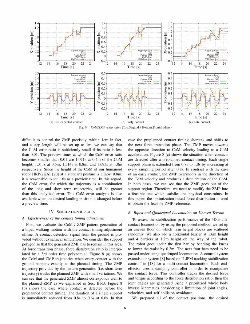
Fig. 8. CoM/ZMP trajectories (Top:Sagittal / Bottom:Frontal plane)

difficult to control the ZMP precisely, within 1cm in fact,and a step length will be set up to 1m, we can say thatthe CoM error ratio is sufficiently small if its ratio is lessthan 0.01. The preview times at which the CoM error ratiobecomes smaller than 0.01 are 1.071s at 0.4m of the CoMheight, 1.311s at 0.6m, 1.514s at 0.8m, and 1.693s at 1.0mrespectively. Since the height of the CoM of our humanoidrobot HRP-2KAI [20] at a standard posture is almost 0.8m,it is reasonable to set 1.6s as a preview time. In this regard,the CoM error, for which the trajectory is a combinationof the long and short term trajectories, will be greaterthan this analytical error. This CoM error analysis is alsoavailable when the desired landing position is changed beforea preview time.

IV. SIMULATION RESULTS

A. Effectiveness of the contact timing adjustment

First, we evaluate the CoM / ZMP pattern generation ofa biped walking motion with the contact timing adjustmentoffline. A contact detection signal from the ground is pro-vided without dynamical simulation. We consider the supportpolygon so that the generated ZMP has to remain in this area.At force transition phase, force distribution ratio is interpo-lated by a 3rd order time polynomial. Figure 8 (a) showsthe CoM and ZMP trajectories when every contact with theground happens exactly at the planned timing. The ZMPtrajectory provided by the pattern generation (i.e. short termtrajectory) tracks the planned ZMP with small variations. Wecan see that the generated ZMP almost corresponds well tothe planned ZMP as we explained in Sec. III-B. Figure 8(b) shows the case where contact is detected before thepreplanned contact timing. The duration of a single supportis immediately reduced from 0.8s to 0.6s at 0.6s. In that

case the preplanned contact timing shortens and shifts tothe next force transition phase. The ZMP moves towardsthe opposite direction to CoM velocity leading to a CoMacceleration. Figure 8 (c) shows the situation when contactsare detected after a preplanned contact timing. Each singlesupport phase is extended from 0.8s to 1.0s by increasing atevery sampling period after 0.8s. In contrast with the caseof an early contact, the ZMP overshoots in the direction ofthe CoM velocity and produces a deceleration of the CoM.In both cases, we can see that the ZMP goes out of thesupport region. Therefore, we need to modify the ZMP intoa feasible one which satisfies the physical constraints. Inthis paper, the optimization-based force distribution is usedto obtain the feasible ZMP reference.

B. Biped and Quadruped Locomotion on Uneven Terrain

To assess the stabilization performance of the 3D multi-contact locomotion by using the proposed method, we set upan uneven floor on which 1cm height blocks are scatteredrandomly. We also add a horizontal barrier at 1.6m heightand 4 barriers at 1.2m height on the way of the robot.The robot goes under the first bar by bending the kneesto lower the waist by 0.2m. The next four bars need to bepassed under using quadruped locomotion. A control systemextends our system [8] based on “LIPM tracking stabilizationcontrol” in [18] for a multi-contact locomotion. Each end-effector uses a damping controller in order to manipulatethe contact force. This controller tracks the desired forceand torque according to the force distribution ratio, then thejoint angles are generated using a prioritized whole bodyinverse kinematics considering a limitation of joint angles,velocities, and self collision avoidance.

We prepared all of the contact positions, the desired

6

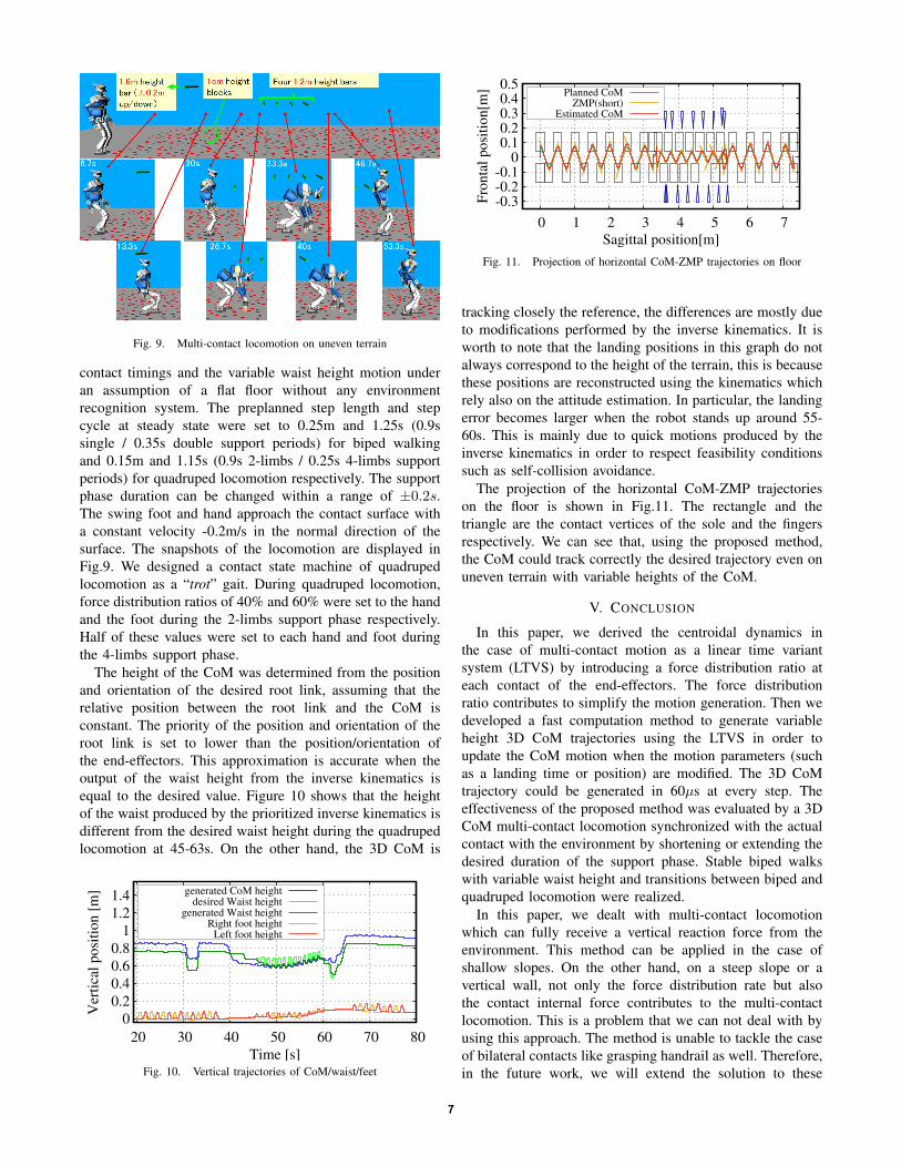
Fig. 9. Multi-contact locomotion on uneven terrain

contact timings and the variable waist height motion underan assumption of a flat floor without any environmentrecognition system. The preplanned step length and stepcycle at steady state were set to 0.25m and 1.25s (0.9ssingle / 0.35s double support periods) for biped walkingand 0.15m and 1.15s (0.9s 2-limbs / 0.25s 4-limbs supportperiods) for quadruped locomotion respectively. The supportphase duration can be changed within a range of ±0.2s.The swing foot and hand approach the contact surface witha constant velocity -0.2m/s in the normal direction of thesurface. The snapshots of the locomotion are displayed inFig.9. We designed a contact state machine of quadrupedlocomotion as a “trot” gait. During quadruped locomotion,force distribution ratios of 40% and 60% were set to the handand the foot during the 2-limbs support phase respectively.Half of these values were set to each hand and foot duringthe 4-limbs support phase.

The height of the CoM was determined from the positionand orientation of the desired root link, assuming that therelative position between the root link and the CoM isconstant. The priority of the position and orientation of theroot link is set to lower than the position/orientation ofthe end-effectors. This approximation is accurate when theoutput of the waist height from the inverse kinematics isequal to the desired value. Figure 10 shows that the heightof the waist produced by the prioritized inverse kinematics isdifferent from the desired waist height during the quadrupedlocomotion at 45-63s. On the other hand, the 3D CoM is

0

0.2

0.4

0.6

0.8

1

1.2

1.4

20 30 40 50 60 70 80

Ver

tica

l p

osi

tion [

m]

Time [s]

generated CoM heightdesired Waist height

generated Waist heightRight foot height

Left foot height

Fig. 10. Vertical trajectories of CoM/waist/feet

-0.3-0.2-0.1

0 0.1 0.2 0.3 0.4 0.5

0 1 2 3 4 5 6 7

Fro

nta

l p

osi

tion[m

]

Sagittal position[m]

Planned CoMZMP(short)

Estimated CoM

Fig. 11. Projection of horizontal CoM-ZMP trajectories on floor

tracking closely the reference, the differences are mostly dueto modifications performed by the inverse kinematics. It isworth to note that the landing positions in this graph do notalways correspond to the height of the terrain, this is becausethese positions are reconstructed using the kinematics whichrely also on the attitude estimation. In particular, the landingerror becomes larger when the robot stands up around 55-60s. This is mainly due to quick motions produced by theinverse kinematics in order to respect feasibility conditionssuch as self-collision avoidance.

The projection of the horizontal CoM-ZMP trajectorieson the floor is shown in Fig.11. The rectangle and thetriangle are the contact vertices of the sole and the fingersrespectively. We can see that, using the proposed method,the CoM could track correctly the desired trajectory even onuneven terrain with variable heights of the CoM.

V. CONCLUSION

In this paper, we derived the centroidal dynamics inthe case of multi-contact motion as a linear time variantsystem (LTVS) by introducing a force distribution ratio ateach contact of the end-effectors. The force distributionratio contributes to simplify the motion generation. Then wedeveloped a fast computation method to generate variableheight 3D CoM trajectories using the LTVS in order toupdate the CoM motion when the motion parameters (suchas a landing time or position) are modified. The 3D CoMtrajectory could be generated in 60µs at every step. Theeffectiveness of the proposed method was evaluated by a 3DCoM multi-contact locomotion synchronized with the actualcontact with the environment by shortening or extending thedesired duration of the support phase. Stable biped walkswith variable waist height and transitions between biped andquadruped locomotion were realized.

In this paper, we dealt with multi-contact locomotionwhich can fully receive a vertical reaction force from theenvironment. This method can be applied in the case ofshallow slopes. On the other hand, on a steep slope or avertical wall, not only the force distribution rate but alsothe contact internal force contributes to the multi-contactlocomotion. This is a problem that we can not deal with byusing this approach. The method is unable to tackle the caseof bilateral contacts like grasping handrail as well. Therefore,in the future work, we will extend the solution to these

7

problems towards more general multi-contact situations.

ACKNOWLEDGMENT

This work was partially supported by NEDO’s “Develop-ment of a highly dependable humanoid robot system that canwork in unstructured environments” project and in part bythe CNRS-AIST-Airbus Joint Research Program (JRP).

REFERENCES

[1] L. Sentis, J. Park, and O. Khatib, “Modeling and Control of Multi-Contact Centers of Pressure and Internal Forces in Humanoid Robots,”in Proc. of IEEE Int. Conf. on Robotics and Automation, pp.453-460,2009.

[2] B. Henze, A. Dietrich, and C. Ott, “An Approach to Combine Bal-ancing with Hierarchical Whole-Body Control for Legged HumanoidRobots,” in IEEE Robotics and Automation Letters, Vol.1, No.2, 2016.

[3] K. Nagasaka, T. Fukushima, and H. Shimomura, “Whole-body controlof a humanoid robot based on generalized inverse dynamics and multi-contact stabilizer that can take account of contact constraints,” inRobotics Symposia (in Japanese), Vol.17, 2012

[4] K. Miura, M. Morisawa, F. Kanehiro, S. Kajita, K. Kaneko and K.Yokoi, “Human-like Walking with Toe Supporting for Humanoids,” inProc. of IEEE Int. Conf. on Intelligent Robots and Systems, pp.4428-4435, 2011.

[5] T. Kamioka, T. Watabe, M. Kanazawa, H. Kaneko, and T. Yoshiike,“Dynamic Gait Transition between Bipedal and Quadrupedal Locomo-tion,” in Proc. of IEEE Int. Conf. on Intelligent Robots and Systems,pp.2195-2201, 2015.

[6] J. Englsberger, C. Ott, and A. A-Schaffer, “Three-dimensional bipedalwalking control based on divergent component of motion,” IEEETransaction of Robotics, Vol. 31, No. 2, pp.884-898, 2015.

[7] T. Koolen, S. Bertrand, G. Thomas, T. D. Boer T. Wu, J. Smith,J. Englsberger, and J. Pratt, “Design of a momentum-based controlframework and application to the humanoid robot atlas,” in Int.Journal of Humanoid Robots, Vol.13, No.1, p.1650007-1 - 1650007-34, 2016.

[8] M. Morisawa, N. Kita, S. Nakaoka, K. Kaneko, S. Kajita, and F.Kanehiro, “Biped locomotion control for uneven terrain with narrowsupport region,” in IEEE/SICE Int. Symposium on System Integration,pp. 3439, 2014.

[9] H. Audren, J. Vaillant, A. Kheddar, A. Escande, K. Kaneko, and E.Yoshida, “Multi-contact Walking Pattern Generation based on ModelPreview Control of 3D COM Accelerations,” in Proc. of IEEE Int.Conf. on Intelligent Robots and Systems, pp.4030-4035, 2013.

[10] M. A. Hopkins, D. W. Hong, A. Leonessa, “Compliant LocomotionUsing Whole-Body Control and Divergent Component of MotionTracking,” in Proc. of IEEE Int. Conf. on Robotics and Automation,pp.5726-5733, 2015.

[11] S. Caron and A. Kheddar, “Multi-contact Walking Pattern Generationbased on Model Preview Control of 3D COM Accelerations,” in Proc.of IEEE Int. Conf. on Humanoid Robots, pp.550-557, 2016.

[12] S. Nozawa, M. Kanazawa, Y. Kakiuchi, K. Okada, T. Yoshiike, and M.Inaba, “Three-dimensional Humanoid Motion Planning Using COMFeasible Region and its Application to Ladder Climbing Tasks,” inProc. of IEEE Int. Conf. on Humanoid Robots, pp.49-56, 2016.

[13] T. Takenaka, T. Matsumoto, T. Yoshiike, T. Hasegawa, S. Shirokura,H. Kaneko and A. Orita, “Real Time Motion Generation and Controlfor Biped Robot -4th Report: Integrated Balance Control-,” in Proc. ofIEEE/RSJ Int. Conf. on Intelligent Robots and Systems, pp.1601-1608,2009.

[14] M. Kanazawa, S. Nozawa, Y. Kakiuchi, Y. Kanemoto, M. Kuroda, K.Okada, M. Inaba and T. Yoshiike, “Robust Vertical Ladder Climbingand Transitioning between Ladder and Catwalk for Humanoid Robots,”in Proc. of IEEE Int. Conf. on Intelligent Robots and Systems, pp.2202-2209, 2015.

[15] A. D. Prete, S. Tonneau and N. Mansard, “Fast Algorithms to TestRobust static Equilibrium for Legged Robots,” in Proc. of IEEE Int.Conf. on Robotics and Automation, pp.1601-1607, 2016.

[16] S. Caron, Q. Cuong and Y. Nakamura, “ZMP support areas for multi-contact mobility under frictional constraints,” IEEE Transaction ofRobotics, Vol. 33, Issue 1, pp.67-80, 2017.

[17] M. Popovic, A. Goswami and H. M. Herr, “Ground reference pointsin legged locomotion: definitions, biological trajectories and controlimplications,” Int. Journal of Robotics Research, Vol.24, No.12,pp.1013-1032, 2005.

[18] S. Kajita, M. Morisawa, K. Miura, S. Nakaoka, K. Harada, K. Kaneko,F. Kanehiro, and K. Yokoi, “Biped walking stabilization based onlinear inverted pendulum tracking,” in Proc. of IEEE/RSJ Int. Conf.on Intelligent Robots and Systems, pp.4489-4496, 2010.

[19] M. Morisawa, F. Kanehiro, K. Kaneko, N. Mansard, J. Sola, E.Yoshida, K. Yokoi, and J-P. Laumond, “Combining Suppression ofthe Disturbance and Reactive Stepping for Recovering Balance,” inProc. of IEEE Int. Conf. on Intelligent Robots and Systems, pp.3150-3156, 2010.

[20] K. Kaneko, M. Morisawa, S. Kajita, S. Nakaoka, T. Sakaguchi, R. Cis-neros, and F. Kanehiro, “Humanoid robot HRP-2 Kai - Improvementof HRP-2 towards disaster response tasks,” in Proc. of IEEE-RAS Int.Conf. on Humanoid Robots, pp.132139, 2015.

8