One Reason Countries Pay Their Debts:Renegotiation and International Trade

Andrew K. Rose*

December 2001

AbstractThis paper estimates the effect of sovereign debt renegotiation on international trade. Sovereigndefault may be associated with a subsequent decline in international trade either becausecreditors want to deter default by debtors, or because trade finance dries up after default. Toestimate the effect, I use an empirical gravity model of bilateral trade and a large panel data setcovering fifty years and more than 200 trading partners. The model controls for a host of factorsthat influence bilateral trade flows, including the incidence of International Monetary Fundprograms. Using the dates of sovereign debt renegotiations conducted through the Paris Club asa proxy measure for sovereign default, I find that renegotiation is associated with aneconomically and statistically significant decline in bilateral trade between a debtor and itscreditors. The decline in bilateral trade is approximately 8 percent a year and persists for aboutfifteen years.

Keywords: empirical, sovereign, default, bilateral, panel, gravity, Paris Club, rescheduling.

JEL Classification Number: F10, F34

Contact: Andrew K. Rose, Haas School of Business,University of California, Berkeley, CA 94720-1900Tel: (510) 642-6609Fax: (510) 642-4700E-mail: arose@haas.berkeley.eduURL: http://haas.berkeley.edu/∼arose

* B.T. Rocca Jr. Professor of International Business, Economic Analysis and Policy Group, HaasSchool of Business at the University of California, Berkeley, NBER Research Associate, andCEPR Research Fellow. I thank: Mike Dooley, Julian di Giovanni, Jonathan Eaton, Ken Rogoff,Phil Suttle, and seminar participants at the European University Institute and the Federal ReserveBank of New York for comments, and the EUI, the FRBNY, the IMF, and the Tel Aviveconomics department for hospitality while I worked on this paper. I owe special thanks toEddie Dekel and Ben Hermalin, who helped write much of the game-theoretic sub-section. Forassistance with the data, I think Eduardo Borensztein, Malvina Pollock, and JerominZettelmeyer. The data set (the part used for the benchmark estimates) and a current version ofthe paper are available at my website. The author worked on this paper while a visiting scholarat the Federal Reserve Bank of New York. The views expressed do not necessarily reflect thoseof the Federal Reserve Bank of New York or the Federal Reserve System.

2

I: Introduction

Why do countries pay their international debts? Three reasons are typically proposed.

First, countries that renege on their debts may have their overseas assets seized by foreign

creditors. Second, countries with poor repayment reputations may be cut off from capital flows

in the future. Third, delinquent countries may suffer reduced benefits of international trade.

While all three penalties are of interest, this paper is concerned with the last explanation. The

first sanction is of limited potency for net debtors with little foreign collateral. A number of

economists (most visibly Bulow and Rogoff) have disputed the importance of future exclusion

from capital markets. The third explanation is widely accepted, but has never been quantified.

The objective of this paper is to estimate empirically the effect of sovereign debt renegotiations

on international trade.

There are at least two reasons why international default may reduce trade in principle.

First, trade credit may naturally shrink after default. Alternatively, creditors may wish to punish

default with reduced trade benefits, in order to discourage future default, or default by third

parties. In practice, default seems to be strongly associated in practice with reduced trade. I use

a large panel data set covering over 200 trading partners over fifty years of data to estimate a

“gravity” model of trade. I show that debt renegotiation is associated with a decline in bilateral

trade that is both economically and statistically significant, adding up to a year’s worth of trade,

although the effect is spread over fifteen years.

The next section presents a theoretical framework to frame the relationship between

sovereign default and international trade, while the third section presents the institutional setting

of sovereign default through debt renegotiations at the Paris Club. Next, the empirical

methodology and data set are discussed. The actual empirical results are presented in the fifth

3

section, which includes sensitivity analysis. The paper finishes with some suggestions for future

work and a brief conclusion.

II: Why Might Sovereign Default Affect Trade?

There is a large literature on the issue of sovereign default; Eaton and Fernandez (1995)

and Obstfeld and Rogoff (1996, chapter 6) provide recent surveys. However, little of it has been

explicitly concerned with the interaction between default and trade. In this section, I provide a

theoretical framework for the empirical analysis that follows.

There are two reasons why sovereign default could affect trade. The more interesting

reason is that a creditor may want to discourage further default (either by the debtor in the future

or by other debtors), with a punishing decline in trade. The more banal reason is that default

may naturally result in a drying up of short-term trade credit, the vehicle used to finance most

international trade. In practice, it is difficult and, for my purposes, unimportant, to differentiate

between these explanations. I explore both briefly below.

Restriction of Trade as an Inducement for Debt Repayment

While the literature provides strong hints that restricted international trade can be used to

encourage debt repayment, formal modeling is relatively rare.1 It is not my intention to provide a

full-fledged model of the interaction between sovereign default and trade. Rather, I provide two

intuitive examples of how sovereign default might be punished by a reduction in international

trade. The first example involves multiple debtors; the creditor restricts trade to punish the

defaulter and thereby deter default by other countries. The second example involves only a

single debtor; trade restrictions are used to deter future default.

4

Trade Restrictions to Deter Default by Other Debtors2

Suppose there are N + 1 countries, of which one is the creditor country and the other are

borrowing countries. Trade between the creditor and debtor n generates surplus of 2T(Xnt) in

period t if trade is unconstrained, where Xnt is the economic state of n at time t. For

convenience, assume the surplus is evenly divided between the creditor and the debtor. Each

period, the borrow must repay d to the creditor (i.e., service its debt). If d is not repaid, then the

creditor can restrict trade, reducing the surplus per country to knT(Xnt), where 0 < kn < 1. The

timing within a period is that debtors simultaneously decide to repay or not, then the creditor

decides whether to take actions against delinquent debtors.

Assume that Xnt is randomly and, for convenience, independently determined each period

from an interval that we normalize to be [0,1]. Let S(X) be the survival function (one minus the

distribution function). Assume T is an increasing function and that T(0) = 0. Let δ be the

common discount factor. For convenience, assume all debtors are identical.

Consider the following strategies for the countries:

• Creditor: Provided it has maintained its reputation to punish, then, in the interactions

with each debtor, set kn = 1 if repaid that period, otherwise set it to kn = k* < 1 (i.e.,

punish). If it has failed to maintain its reputation, then set kn = 1 regardless of repayment.

• Debtor: If the creditor has always punished non-repayers or there has yet to be an

instance of non-repayment, then repay if T – d > k*T and default otherwise. If the

creditor has ever failed to punish non-repayers, then default regardless of T.

If the creditor fails to punish, then the rest of the game is clearly subgame perfect: the

creditor anticipates that it can not affect debtors’ behavior, so there is no point to punishment,

5

given that punishing also punishes the creditor. Without punishment, there is no motive to repay

(and hence, no debt).

It is only required to verify that the strategies can be equilibrium strategies. If the debtor

believes that the creditor will punish, then the strategy for the debtor is clearly rational. For the

creditor, the question is whether to suffer the short-run cost of punishing to maintain its

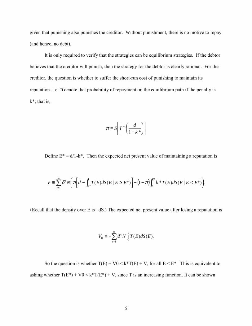
reputation. Let π denote that probability of repayment on the equilibrium path if the penalty is

k*; that is,

.*1

1

−= −

kdTSπ

Define E* ≡ d/1-k*. Then the expected net present value of maintaining a reputation is

( )∑ ∫∫∞

=

<−−

≥−≡

1

*

0

1

*.*)|()(*1*)|()(

t

E

E

t EEEdSETkEEEdSETdNV ππδ

(Recall that the density over E is –dS.) The expected net present value after losing a reputation is

∑ ∫∞

=

−≡1

1

00 ).()(t

t EdSETNV δ

So the question is whether T(E) + V0 < k*T(E) + V, for all E < E*. This is equivalent to

asking whether T(E*) + V0 < k*T(E*) + V, since T is an increasing function. It can be shown

6

that if there exists a k* such that π > ½, then there is an N such that this inequality holds; that is,

such that punishing is a credible threat.

Thus, the creditor uses trade restrictions to punish the defaulting country, and thereby

deter default by other debtors.

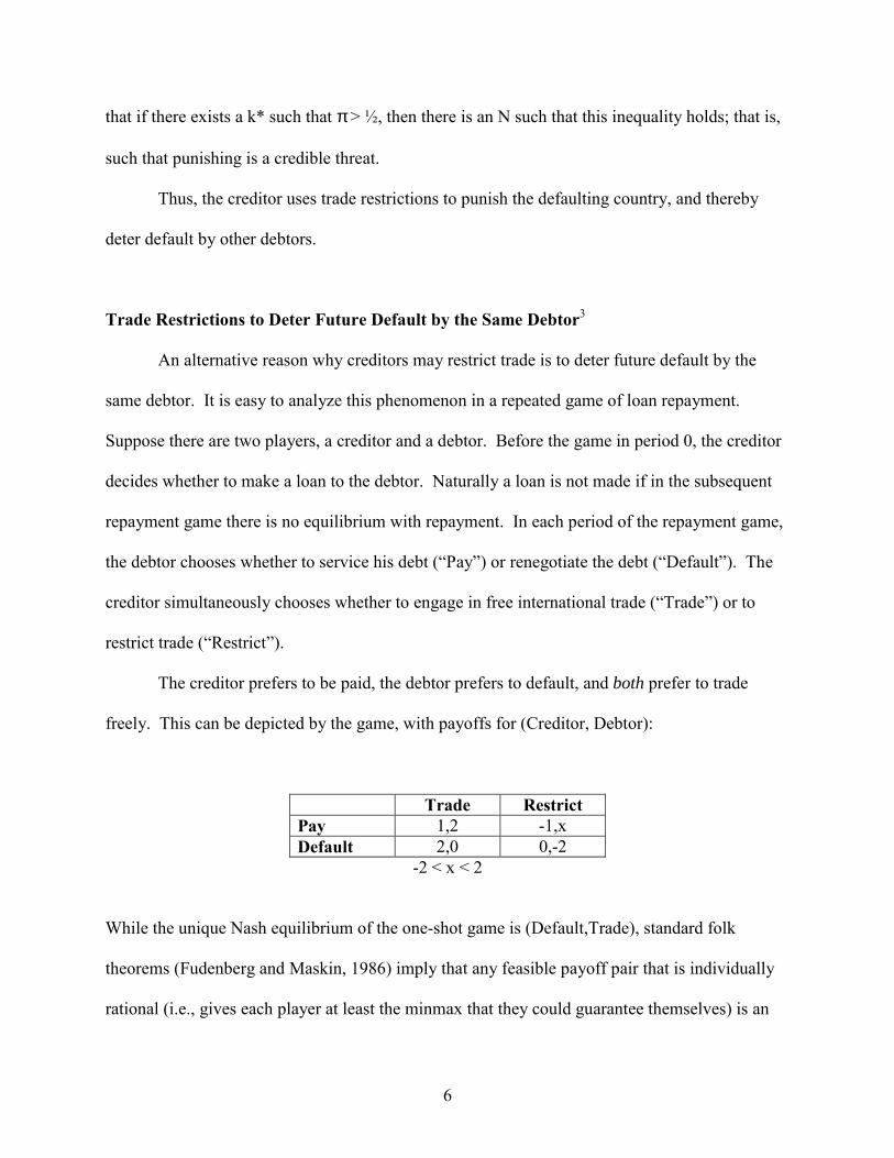
Trade Restrictions to Deter Future Default by the Same Debtor3

An alternative reason why creditors may restrict trade is to deter future default by the

same debtor. It is easy to analyze this phenomenon in a repeated game of loan repayment.

Suppose there are two players, a creditor and a debtor. Before the game in period 0, the creditor

decides whether to make a loan to the debtor. Naturally a loan is not made if in the subsequent

repayment game there is no equilibrium with repayment. In each period of the repayment game,

the debtor chooses whether to service his debt (“Pay”) or renegotiate the debt (“Default”). The

creditor simultaneously chooses whether to engage in free international trade (“Trade”) or to

restrict trade (“Restrict”).

The creditor prefers to be paid, the debtor prefers to default, and both prefer to trade

freely. This can be depicted by the game, with payoffs for (Creditor, Debtor):

Trade Restrict Pay 1,2 -1,x Default 2,0 0,-2

-2 < x < 2

While the unique Nash equilibrium of the one-shot game is (Default,Trade), standard folk

theorems (Fudenberg and Maskin, 1986) imply that any feasible payoff pair that is individually

rational (i.e., gives each player at least the minmax that they could guarantee themselves) is an

7

equilibrium payoff of the infinitely repeated game with sufficiently players (i.e., discount rate δ

close enough to 1). In this game the minmax is (0,0) and, in particular, (1,2) can be sustained by

the carrot-stick equilibrium in which (Pay, Trade) is played along the equilibrium path and

deviations are punished by playing (Default, Restrict) for an appropriate number of periods.4

The drawback of such a model is that in equilibrium, no punishments should be observed.

In the spirit of Green and Porter (1984) one can therefore allow for imperfect observability

(although of a different form). In particular consider a model with two states, Good and Bad,

where it is very costly for the debtor to service debt in the bad state. The payoffs are as above,

except that the debtor’s payoffs when paying are reduced by some large M. The creditor cannot

verify the state, although naturally the debtor observes the state. The state is independently

drawn each period, where Good has a probability p in (p*,1).5

The equilibrium above can be simply modified to be a perfect public equilibrium

(Fudenberg, Levine and Maskin, 1994) in which punishments are observed along the equilibrium

path. In particular, for appropriate values of δ<1, p*<1 and M, then the above will not be an

equilibrium, since the debtor will default. Nevertheless, it will be equilibrium for the debtor to

pay except in bad states, and to default in bad states. Default results in a single period of (Pay,

Trade) followed by a punishment phase, which is a certain number of periods of (Default,

Restrict).6 Thus, the equilibrium path will involve intervals of (Pay, Trade), broken by a period

of (Default, Trade) which is then punished by an interval of (Default, Restrict) and then either a

return to (Pay, Trade) (with probability p) or, with probability (1-p) to another (Default, Trade),

instigating another (Default, Restrict).7

Thus, in this example the creditor uses trade restrictions to punish the defaulting country,

and thereby deter future default by the debtor.

8

Default and Trade Credit

The two examples show that it is possible that trade restrictions can be used to punish and

deter default. But a fall in trade after sovereign default need not be a deliberate overt act of

retaliation. Indeed, as a result of sovereign default or risk creditor countries have never, to my

knowledge, used formal legal sanctions.8 Instead, any negative effect may be simply the result

of the drying-up of short-term trade credit.9

Kaletsky (1985, pp 36-38) argues: “The interruption of trade finance might turn out to be

the heaviest penalty for a defaulter. Trade finance is a critical issue because most trade is

conducted on a credit basis of one kind or another … trade finance could be the Achilles’ heel of

a default strategy.”10 Consistent with this, Cohen (1991, p1) states: “A defaulting country first

loses access to its trade credit… Trade, in general, becomes difficult, exporting is tricky, and so

is paying for its imports.” Rogoff (1999, p 31) writes “The strongest weapon of disgruntled

creditors, perhaps, is the ability to interfere with short-term credits that are the lifeblood of

international trade.” Alternatively, insurance rates for international trade (especially those

offered by official agencies) may rise as a result of default.11 Thus, there are reasons to expect a

negative impact of debt renegotiation on international trade above and beyond those of deliberate

government policy.12

Discussion

It is not necessary to argue that reduced international trade is the only deterrent to

sovereign default; the “pure reputation” effects disputed by Bulow and Rogoff (1989a,b) may

also be present. Nevertheless, there is little evidence that alternative mechanisms are very

9

important. For instance, Lindert and Morton (1989, p 231) examine historical rate of returns and

find “A clear result from the history of rates of return on sovereign debt relates to the ex post

treatment of those who fell into arrears: The only ones punished were few countries defaulting in

isolation before 1918. The majority of non repayers ‘escaped’ punishment…” They later argue

(p 234): “Countries that had defaulted in the past were significantly more likely to become

problem debtors again. Yet defaulting governments have seldom been punished, either with

direct sanctions or with discriminatory denial of later credit.”13

It seems clear that there are reasons to believe that sovereign default may lead to a

decline in international trade, either as a punishment for and deterrent to further default, or

simply because of more costly trade finance and/or insurance. For my purposes, all that is

important is that there is some reason for debtors to fear the consequences of default for their

international trade. Whether there is any significant linkage in practice is ultimately an empirical

question. I now turn to that task. First, it is important to discuss the institutional setting of

sovereign default.

III: Sovereign Debt Renegotiation in Practice

In practice, it is rare for a country simply to default on (let alone repudiate) its

international financial obligations. Instead, it typically renegotiates its debts, usually through the

“Paris Club.” In this section, I provide a brief overview of the debt renegotiation process. More

information on the Paris Club is provided by Sevigny (1990), Eichengreen and Portes (1995),

and the website of the Paris Club.14

The Paris Club is an informal group of official creditors that meets approximately ten

times a year to discuss issues associated with external debts of developing countries, and

10

renegotiate these debts.15 The Paris Club began with the 1956 renegotiation of Argentina’s

external debt, and has since reached over 335 agreements with over 75 debtor countries; these

collectively total over $375 billion. The French Treasury provides a small secretariat for the

club.

The Paris Club is informal and has no legal basis or status; instead it adheres to a set of

principles. Three of the key principles are particularly germane. First, all decisions by creditors

are taken by consensus, ensuring “creditor solidarity.” Second, the Paris Club preserves

“comparability of treatment” between all creditors. In particular, it is expected that Paris Club

members, non-members, and private creditors (notably banks) be treated comparably by the

debtor country, to ensure equitable burden sharing. The only exceptions are the international

financial institutions such as the IMF and World Bank that are treated as preferred, though they

are often expected to provide new money. Third, the Paris Club prefers that deals be negotiated

only for countries that are engaged in an IMF-approved program, complete with appropriate

conditionality.

The relationship with the IMF is important. An IMF program is a litmus test for

“imminent default,” and thus ensures that renegotiation is warranted. More importantly, an IMF

program is a means to implementing the reforms required to resolve the underlying payments

difficulties. Thus an IMF program usually precedes a Paris Club deal. But the dance is

complicated, since the IMF typically agrees to a program only with the implicit assurance from

the Paris Club that temporary debt relief from the creditors will be forthcoming, in order to

ensure IMF repayment.16

Paris Club agreements apply to public sector debt as well as private debt guaranteed by

the public sector.17 The debts considered are only those granted before a “cutoff date” which is

11

not changed in subsequent negotiations; this division of debts is intended to help restoration of

the flow of credit. It is important to note that only medium and long-term debts are rescheduled.

To quote the Paris Club: “Short term debt (debt with a maturity of one year or less) is excluded

from the treatments, as their restructuring can create a significant disruption of the capacity of

the debtor country to participate in international trade.”18 The overt attempt by the Paris Club to

protect trade from default is an additional reason why determining the relationship between trade

and default is essentially an empirical matter.

Paris Club membership is open to all creditor governments that accept its practices.

However, while developing countries occasionally participate in the negotiations, the core

members are large OECD countries.19 In order to reduce the costs of renegotiation, only creditor

countries with debts exceeding a small “de minimis” level negotiate (creditors sometimes

participate as observers if their levels are lower than the de minimis level). Thus, participation

varies with both the debtor and time. The Paris Club operates quickly in practice; negotiations

begin soon after an IMF program begins and are typically concluded within six to eight

months.20

The Paris Club provides four different types of renegotiation. “Classic terms” include:

five years of grace; semi-annual principal repayment terms in years six to ten; and a moratorium

interest rate which is designed to keep the net present value of the debt intact. Three sets of

additional terms have been made available more recently; all involve a grant element that

reduces the net present value of the debt. “Toronto terms” were created in 1988 to facilitate debt

reduction for very low-income countries. These were superceded in 1991 by “London terms”

which were in turn replaced in 1994 by “Naples terms.” “Houston terms” were created in 1990

for low-middle income countries. In 1996 the HIPC initiative (for Heavily Indebted Poor

12

Countries) became available under “Lyon Terms” which were subsequently modified to

“Cologne terms”. In this paper I use only “classic” Paris Club agreements, which account for the

majority of all Paris Club deals. Since they do not involve any (intended) grant element, they are

most appropriate in isolating any effects of debt renegotiations on trade. (It would be interesting

to investigate Paris Club deals with a grant element, although the small sample size makes this a

difficult endeavor at present).

Paris Club agreements seem to be the most appropriate dates for measuring sovereign

default. The only potential alternative dating scheme would use the onset of arrears of

international payments of interest, principal, or both. This seems an inferior measure. There

were 283 Paris Club deals through 1997 (some of which were not “classic”), and 163 spells of

arrears that together spanned some 2000 country-year observations. The overlap between the

onset of arrears and Paris Club deals is poor, even within a year or two. While some of the

arrears spells were clearly defaults, some were officially or quietly encouraged so that the arrears

were strictly technical (e.g., between an IMF program and the conclusion of a Paris Club deal).

Further, arrears were rarely absolute; partial debt service was routinely continued during periods

of arrears and was usually comparable to (or higher than) the size of arrears. This makes it

difficult to measure the nature and scope of default simply though using the presence of arrears.

Further, arrears is a multilateral concept, whereas Paris Club information is available on a

bilateral basis. For all these reasons, I use the dates of Paris Club deals to date sovereign debt

renegotiation.

13

IV: Empirical Methodology and Data

Estimation Strategy

I use a conventional gravity model to model bilateral trade flows, augmented with a

number of extra controls:

ln(Xijt) = β0 + β1ln(YiYj)t + β2ln(YiYj/PopiPopj)t + β3lnDij + β4Langij + β5Contij

+ β6FTAijt + β7Landlij + β8Islandij +β9ln(AreaiAreaj) + β10ComColij

+ β11CurColijt + β12Colonyij + β13ComNatij + β14CUijt

+ β15,0IMFijt + ΣKβ15,kIMFijt-k + φRENEGijt + ΣMφmRENEGijt-m + εijt

where i and j denotes countries, t denotes time, and the variables are defined as:

• Xijt denotes the average value of real bilateral trade between i and j at time t,

• Y is real GDP,

• Pop is population,

• Dij is the distance between i and j,

• Lang is a binary variable which is unity if i and j have a common language,

• Cont is a binary variable which is unity if i and j share a land border,

• FTA is a binary variable which is unity if i and j belong to the same regional trade

agreement,

• Landl is the number of landlocked countries in the country-pair dyad (0, 1, or 2).

• Island is the number of island nations in the pair (0, 1, or 2),

• Area is the land mass of the country,

14

• ComCol is a binary variable which is unity if i and j were ever colonies after 1945 with the

same colonizer,

• CurCol is a binary variable which is unity if i and j are colonies at time t,

• Colony is a binary variable which is unity if i ever colonized j or vice versa,

• ComNat is a binary variable which is unity if i and j remained part of the same nation during

the sample (e.g., France and Guadeloupe, or the UK and Bermuda),

• CU is a binary variable which is unity if i and j use the same currency at time t,

• IMF is one/two if one/both of i or/and j began an IMF program at t and zero otherwise,

• RENEG is a binary variable which is unity if i and j renegotiated international debt at time t

and zero otherwise,

• K and M are unknown lag lengths,

• β are a set of nuisance coefficients, and

• ε represents the myriad other influences on bilateral trade, assumed to be well behaved.

The coefficients of interest to me are {φ}, the effect of current and lagged debt renegotiations

on trade.

I estimate the model with both fixed and random effects panel data estimators. The fixed-

effects (“within”) estimator is equivalent to adding a comprehensive set of (11,178) country pair-

specific intercepts to the estimating equation. This ensures consistent estimation of φ under a

wide range of circumstances, but may not be efficient.21 GLS/random-effects (“variance

components”) can be more efficient, but is well known to be consistent in a more restricted set of

circumstances.22

15

The Data Set

The trade data used in this paper is taken from the “Direction of Trade” data set

developed in CD-ROM form by the International Monetary Fund (IMF); the same data set is

used by Glick and Rose (2002). The data set covers bilateral trade between all 217 entities

measured by the IMF between 1948 and 1997 (thought many observations are missing). Not all

of the trading partners are “countries” in the conventional sense of the word; colonies (e.g.,

Bermuda), territories (e.g., Guam), overseas departments (e.g., Guadeloupe), countries that

gained their independence (e.g., Guinea-Bissau), and so forth are all included. I use the term

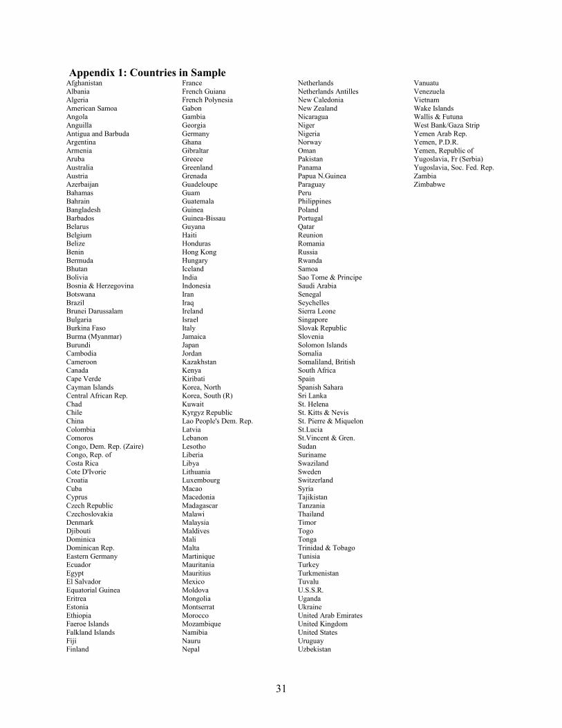
“country” simply for convenience. The countries are listed in Appendix 1. Bilateral trade on

FOB exports and CIF imports is recorded in American dollars; I deflate trade by the American

CPI.23 I create an average value of bilateral trade between a pair of countries by averaging all

four trade flows available.24

To this data set, I add a number of other variables that are necessary to estimate the

gravity model. Population and real GDP data (in constant dollars) are taken from three sources.

Wherever possible, I use “World Development Indicators” (taken from the World Bank’s WDI

2000 CD-ROM) data. When the data are unavailable from the World Bank, I fill in missing

observations with comparables from the Penn World Table Mark 5.6, and (when all else fails),

from the IMF’s “International Financial Statistics”.25 The series have been checked and

corrected for errors.

I exploit the CIA’s “World Factbook” for a number of country-specific variables. These

include: latitude and longitude, land area (in square kilometers), landlocked and island status,

physically contiguous neighbors, language, colonizers, and dates of independence.26 I use these

to create great-circle distance (in miles) and other controls. I obtain data from the World Trade

16

Organization to create an indicator of regional trade agreements, and include: EEC/EC/EU; US-

Israel FTA; NAFTA; CARICOM; PATCRA; ANZCERTA; and Mercosur.27 Currency union

pairs are taken from Glick and Rose (2002).

The Paris Club’s website provides data on all agreements including: the date; the cutoff

date; the type of treatment (Classic/Naples, etc.); the list of participating creditor and observer

countries; the amount of debt treated; the current status of the agreement; and so forth. I use

these data in order to construct my dummy variable for debt renegotiations, RENEG, which is

unity in the year when a creditor-debtor pair was involved in a Paris Club deal and zero

otherwise.28

“Classic” Paris Club agreements are almost always conditioned on IMF programs; in my

sample, over eighty percent of Paris Club agreements coincide with an IMF program signed in

the same year.29 However, not all IMF programs are associated with Paris Club agreements.

Indeed, while there were 283 Paris Club deals though 1997 (of which 163 were “classic”), there

were 898 IMF programs initiated during the same time. (Of these, over 80% (739) were “Stand-

bys Arrangements,” designed to address short-term payments imbalances.30) Since the

implementation of an IMF program is often associated with economic trauma and/or reform, it is

important to condition on the existence of an IMF program in determining the additional

marginal effect of any debt renegotiations.31 My variable, IMFijt is a dummy variable that is

unity if either country i or j initiated an IMF program (of any type) during year t. It takes on a

value of two if both i and j begin an IMF program in the year, and zero otherwise.

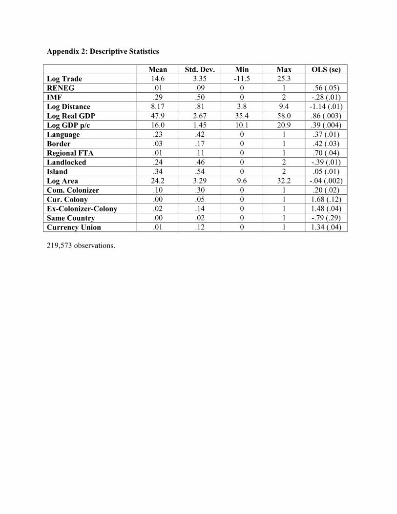
Descriptive statistics for the variables are provided in Appendix 2, along with OLS

coefficients from a simple regression of the log of trade on the contemporaneous regressors (and

an unrecorded intercept); Appendix 3 tabulates simple bivariate correlations. It is interesting to

17

note that the OLS coefficient for renegotiation is positive. Negative estimates (which are

presented below) manifestly depend on a more sophisticated estimator that takes into account the

panel nature of the data set. It is also worth noting that the simple correlation between Paris

Club negotiations and trade is positive; any negative effect relies on conditioning and/or a more

sophisticated estimator. Further, the incidence of bilateral Paris Club negotiations has only low

correlations with the other (nuisance) variables. While the correlations are statistically

significant given the sample size, none exceeds .1 in magnitude.

V: Empirical Results

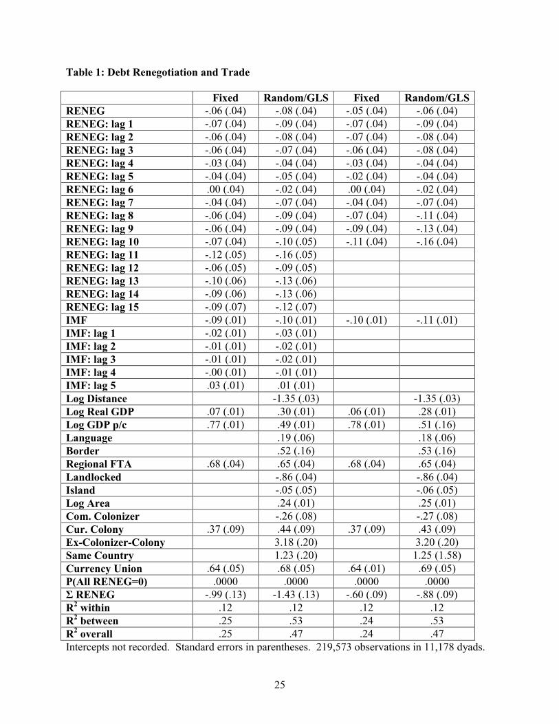
Benchmark Results

Benchmark results are reported in Table 1. In the middle of the table, I tabulate fixed-

and random-effects estimates for an empirical model with contemporaneous and fifteen lags of

the dummy variable for debt renegotiation, five lags of IMF program inception (i.e., K=5,

M=15).

The model works well in a number of senses. The standard “gravity” effects are present;

countries that are further apart geographically trade less, while larger and richer pairs of

countries trade more. Countries that share a common currency, a common language, a common

border, or membership in a regional free trade agreement trade more. Landlocked countries and

islands trade less, and most of the colonial effects are large and positive. Almost all these effects

are economically and statistically significant. The model also explains a reasonable percentage

of the data variation. The inception of IMF programs is associated with a drop in bilateral trade

of about ten percent, holding other things equal. This effect is economically and statistically

18

large, but transient. After around three years this effect dies away, and turns slightly positive

after five years.

Above and beyond all these (mostly) conventional effects on bilateral trade, debt

renegotiations seem to have a substantial negative effect on international trade. The effect is

somewhat sensitive to the exact method of estimation; the fixed effects estimator indicates a

decline of trade of about seven percent annually, while the GLS estimator shows a larger effect

of nine percent. Both effects are highly persistent, lasting around fifteen years at more or less

constant levels. While the individual φ coefficients are often statistically insignificant because of

multicollinearity, the hypothesis that debt renegotiations have no effect on trade can be rejected

at any reasonable significance level. Further, the cumulative effect of renegotiations on trade is

also large negative and significant. The effect averages about eight percent annually and persists

for about fifteen years. The two columns at the right of Table 1 show that these effects are not

especially sensitive to the exact specification of the lag length; eliminating the lags of IMF

program inception and dropping the last five renegotiation lags does not destroy the negative

effect of debt renegotiation on trade.

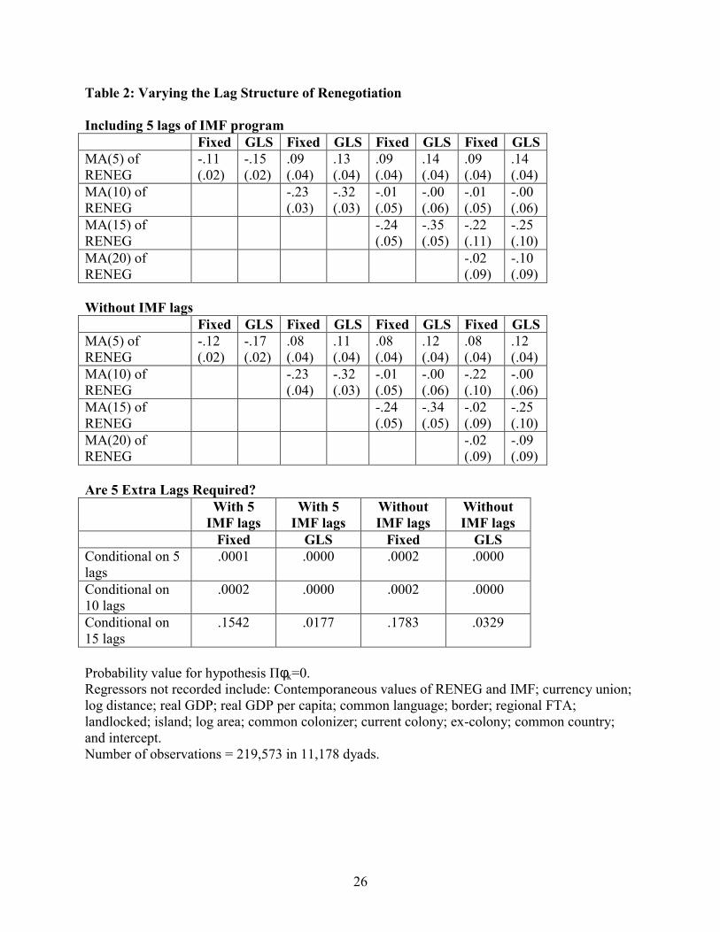
Lag Length

The appropriate number of lags of debt renegotiation (M) is unknown. Does uncertainy

about M affect any economic conclusions? No. Table 2 explores the effects of different lag

lengths for the debt renegotiation variable. To simplify the analysis, I impose equality on the

coefficients of lagged debt renegotiations. Thus in the left-hand columns of the top panel of

Table 2, I tabulate the fixed- and random-effects estimates of φk for k=1,…,5 where a single

coefficient is estimated for lags of RENEG between one and five. (Coefficients for the

19

contemporaneous and 5 values of IMF program inception and the other nuisance coefficients are

not reported.) In the next columns to the right, I add a tenth-order term to the fifth-order term.32

At the extreme right of the table, I have four separate coefficients, representing lags up to twenty,

up to fifteen, up to ten, and up to five years after debt renegotiations. The top panel includes five

lags of IMF program inception as well as the contemporaneous impact, while the middle panel

reports the analogous statistics when IMF program inception is modeled as only having a

contemporaneous effect.

The results indicate that debt renegotiations have a persistent effect, one that seems to last

about fifteen years. This result does not depend very strongly on which estimation method is

used, or whether lags of the IMF variable are included. The bottom panel of Table 2 confirms

this. It reports probability values for the hypothesis Πmφm=0 for values of m>M, where

M=5,10,15. As M rises to 15, the hypothesis that an additional five lags are not required

becomes reasonable with the within estimator (though it is more marginal with GLS). Including

fifteen lags of debt renegotiation and five of the IMF variable seems both intuitively and

statistically reasonable. Still, it is inappropriate to place much confidence in the exact lag length,

given that many debt renegotiations have only taken place in the last fifteen years.

In passing, I note that adding one or two leads of Paris Club renegotiation has no effect

on the economic or statistical significance of debt renegotiation; the leads themselves are

insignificant. This provides further evidence that the Paris Club dates are appropriate dates for

debt renegotiation.

Censoring, Simultaneity and Sensitivity Analysis

20

Trade is bounded below by zero, so a technique that takes this constraint into account

may be preferable to my default estimators, which are both linear. Thus Table 3 presents a

random-effects panel Tobit estimator.33 Reassuringly, the results are quite similar to those of

Table 1 (though they are considerably more computationally demanding).34

Debt renegotiation may be caused by shocks that also cause trade flows to shrink; that is,

the estimation strategy may be biased because trade and debt renegotiation are simultaneously

determined by some other factor that has been omitted from the statistical analysis. While

theoretically plausible, there is no direct evidence indicating that this issue is important in

practice. A long unsuccessful research program attempted to find variables systematically

associated with sovereign default in order to create leading and contemporaneous indicators of

default. Babbel (1996) provides an annotated bibliography of the literature, while Eaton,

Gersovitz and Stiglitz (1986) provide an earlier survey.

Still, there is no reason in principle not to analyze regressors that are potentially

associated with sovereign default. I proceed by using potential causes of default as instrumental

variables in the trade equation. Table 3 uses three instrumental variables: 1) the government

budget surplus/deficit (expressed as a percentage of GDP); 2) the CPI inflation rate; and 3) the

current account surplus/deficit (percentage of GDP). In each case I use values (for both i and j)

of these instrumental variables for contemporaneous debt renegotiation and the onset of IMF

programs. All the regressors were taken from the World Bank’s WDI 2000 CD-ROM.

Reassuringly, both fixed- and random-effects indicate that simultaneity bias is not

responsible for the negative effect of renegotiation on trade; both the joint and the cumulatively

negative effects remain significant. Nevertheless, the IV estimates are obtained only with a

dramatic reduction in observations since the macroeconomic instrumental variables are missing

21

for many of the original observations.35 Further, the instrumental variables are poor in the sense

that they deliver imprecise estimates; while Πmφm and Σmφm remain negative and significant, the

standard errors are much larger.

Table 4 performs a variety of sensitivity experiments with respect to the sample. It

reports probability-values for a key hypothesis, namely Πmφm=0 ∀ m, as well as the point

estimate of Σmφm, along with an appropriate standard error. The statistics are reported for both

fixed- and random-effects estimators for four different samples: 1) the default entire sample; 2)

the sample without the 1990s; 3) the sample without African observations; and 4) the sample

without Latin-American observations. All the evidence indicates that debt renegotiation has a

statistically significant effect on trade, and that the cumulative effect is negative. For one of the

perturbations (when the fixed effects estimator is used without the 1990s), the cumulative effect

is negative but with a t-statistic of unity.

To summarize: the finding that debt renegotiation seems to affect trade aversely seems

robust to uncertainty with respect to lag lengths, censoring, simultaneity, and the exact sample.

Trade Diversion

There seems to be evidence that countries which default engage in less bilateral trade

with their creditors for a number of years after renegotiation. The costs of this reduced trade to

the debtor may be alleviated if trade is merely diverted from creditor countries to others. Thus it

is important to test for trade diversion after debt renegotiation.

I test for trade diversion by adding to the default equation, contemporaneous and lagged

values of a dummy variable that is unity if (at least) one of the countries rescheduled its debt but

the pair of countries was not directly involved in a renegotiation. For instance, Albania

22

rescheduled debt with Austria in 1993, but not with Australia (since Australia is a permanent

member of the Paris Club, this implies that its Albanian assets did not exceed the de minimis

level). My variable “RENEG” is one for Albania-Austria in 1993, but zero for Albania-

Australia; my variable “DIVERT” is exactly the opposite. A positive coefficient for DIVERT

indicates that (e.g., Albanian) trade is diverted away from creditors (e.g., Austria) towards non-

creditors (e.g., Australia).

Table 5 adds contemporaneous and lagged values of DIVERT. Independent of how

many lags of DIVERT are included, its contemporaneous value has a significantly negative

coefficient. Thus the trade of a debtor not only follows with its creditors at the time of

renegotiation, it falls with other countries as well. But it is interesting to note that this negative

effect is much less persistent than that of RESCHED. It turns positive within a couple of years

using the fixed-effects estimator, and within five years using the random-effects estimator. The

exact results are sensitive to both the estimator and the number of lags used, so that it is not

possible to conclude with any confidence whether or not there has been any trade diversion. But

it is clear that trade between debtors and non-creditors is not as dramatically affected by

renegotiation as trade between debtors and creditors.36 This pushes one towards the hypothesis

that creditor countries are seeking to punish default, since trade credit might be expected to dry

up uniformly.

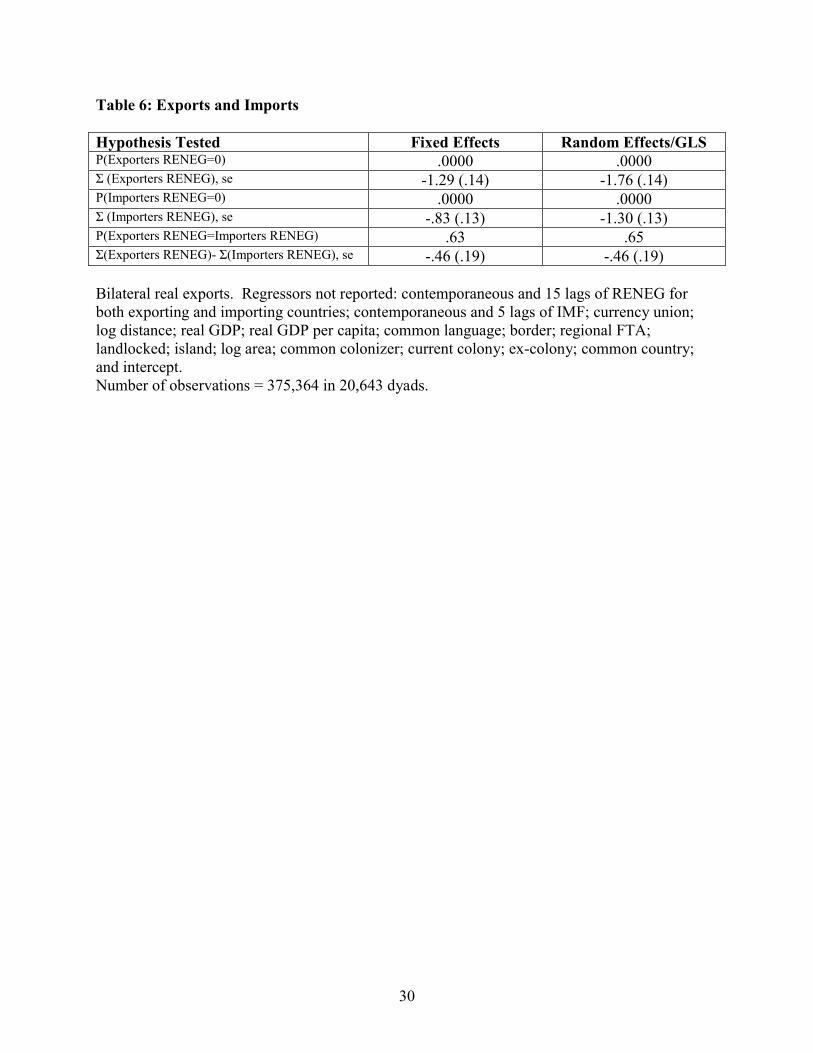
Differential Effects on Exports and Imports

Thus far the analysis has focused on total bilateral trade between a pair of countries,

rather than on exports and imports separately. But there is no reason why default need have the

23

same effect on a defaulting country’s exports and imports. I explore this possibility further in

Table 6.

Table 6 is based on estimation of bilateral export flows, rather than total bilateral trade

flows. Instead of using a single dummy variable to indicate a Paris Club deal that involved in the

pair of countries (and fifteen of its lags), I include two variables (and their lags); one for default

by the exporting country, and another for default by the importer. The other nuisance variables

are included, and results are, as usual, reported for both fixed- and random-effects estimators.

The results indicate that Paris Club renegotiation has similar effects on both exporting

and importing countries. As is clear from the first two rows, the joint effect of the

contemporaneous and (fifteen) lagged coefficients of renegotiation on exports is highly

statistically significant for both estimators, while the cumulative effect is economically and

statistically large. The middle rows indicate that much the same effects characterize imports,

though the cumulative effects are smaller. At the bottom, I test two hypotheses. The second line

from the bottom is a test of the hypothesis that the joint effect on exports is equal to the joint

effect of imports; that hypothesis cannot be rejected at standard significance levels. Still, the

cumulative effect on exports is somewhat larger than the effect on imports, as is clear from the

last line.

To summarize, the effects of default on exports seem somewhat higher than those on

imports. Still, the most striking result is really that default has a substantive effect on trade.

Other Effects

I have searched for other signs that debt renegotiation dampens international trade by

examining other aspects of Paris Club deals. However, there seems to be only weak evidence

24

that the dollar size of the Paris Club deal, the length of time since the last renegotiation, or the

number of renegotiations has an impact on trade, once other factors have been taken into

account.37

VI: Conclusion

I have found that the renegotiation of international debt through the Paris Club is

associated with a decline in bilateral trade between debtors and creditors. The reduction in trade

is economically and statistically significant. While the results are somewhat sensitive to the

exact specification, trade falls by about eight percent a year for around fifteen years. That is,

international default has negative consequences for trade. This result is robust to a number of

econometric perturbations concerning lag length, treatment of simultaneity, censoring and

sample size. There is weak evidence of trade diversion, and the exports of defaulters are hit

somewhat harder than imports.

It would be interesting to extend this analysis to cover “London Club” negotiations

between debtors and private sector banks. The primary obstacle to this lies in determining the

default dates. London Club activity proceeds with a much longer lag than does the Paris Club,

since the bank advisory committees require near or total unanimity from a more heterogeneous

group than the Paris Club; Eichengreen and Portes (1995) provide more discussion.

I have not identified whether the effect of default on international trade appear because of

a natural shrinking of trade finance or because creditors seek to punish and deter default. While

both seem plausible, the evidence of trade diversion indirectly supports the

punishment/deterrence theory. This is another natural project for future research.

25

Table 1: Debt Renegotiation and Trade

Fixed Random/GLS Fixed Random/GLSRENEG -.06 (.04) -.08 (.04) -.05 (.04) -.06 (.04) RENEG: lag 1 -.07 (.04) -.09 (.04) -.07 (.04) -.09 (.04) RENEG: lag 2 -.06 (.04) -.08 (.04) -.07 (.04) -.08 (.04) RENEG: lag 3 -.06 (.04) -.07 (.04) -.06 (.04) -.08 (.04) RENEG: lag 4 -.03 (.04) -.04 (.04) -.03 (.04) -.04 (.04) RENEG: lag 5 -.04 (.04) -.05 (.04) -.02 (.04) -.04 (.04) RENEG: lag 6 .00 (.04) -.02 (.04) .00 (.04) -.02 (.04) RENEG: lag 7 -.04 (.04) -.07 (.04) -.04 (.04) -.07 (.04) RENEG: lag 8 -.06 (.04) -.09 (.04) -.07 (.04) -.11 (.04) RENEG: lag 9 -.06 (.04) -.09 (.04) -.09 (.04) -.13 (.04) RENEG: lag 10 -.07 (.04) -.10 (.05) -.11 (.04) -.16 (.04) RENEG: lag 11 -.12 (.05) -.16 (.05) RENEG: lag 12 -.06 (.05) -.09 (.05) RENEG: lag 13 -.10 (.06) -.13 (.06) RENEG: lag 14 -.09 (.06) -.13 (.06) RENEG: lag 15 -.09 (.07) -.12 (.07) IMF -.09 (.01) -.10 (.01) -.10 (.01) -.11 (.01) IMF: lag 1 -.02 (.01) -.03 (.01) IMF: lag 2 -.01 (.01) -.02 (.01) IMF: lag 3 -.01 (.01) -.02 (.01) IMF: lag 4 -.00 (.01) -.01 (.01) IMF: lag 5 .03 (.01) .01 (.01) Log Distance -1.35 (.03) -1.35 (.03) Log Real GDP .07 (.01) .30 (.01) .06 (.01) .28 (.01) Log GDP p/c .77 (.01) .49 (.01) .78 (.01) .51 (.16) Language .19 (.06) .18 (.06) Border .52 (.16) .53 (.16) Regional FTA .68 (.04) .65 (.04) .68 (.04) .65 (.04) Landlocked -.86 (.04) -.86 (.04) Island -.05 (.05) -.06 (.05) Log Area .24 (.01) .25 (.01) Com. Colonizer -.26 (.08) -.27 (.08) Cur. Colony .37 (.09) .44 (.09) .37 (.09) .43 (.09) Ex-Colonizer-Colony 3.18 (.20) 3.20 (.20) Same Country 1.23 (.20) 1.25 (1.58) Currency Union .64 (.05) .68 (.05) .64 (.01) .69 (.05) P(All RENEG=0) .0000 .0000 .0000 .0000 Σ RENEG -.99 (.13) -1.43 (.13) -.60 (.09) -.88 (.09) R2 within .12 .12 .12 .12 R2 between .25 .53 .24 .53 R2 overall .25 .47 .24 .47 Intercepts not recorded. Standard errors in parentheses. 219,573 observations in 11,178 dyads.

26

Table 2: Varying the Lag Structure of Renegotiation Including 5 lags of IMF program Fixed GLS Fixed GLS Fixed GLS Fixed GLS MA(5) of RENEG

-.11 (.02)

-.15 (.02)

.09 (.04)

.13 (.04)

.09 (.04)

.14 (.04)

.09 (.04)

.14 (.04)

MA(10) of RENEG

-.23 (.03)

-.32 (.03)

-.01 (.05)

-.00 (.06)

-.01 (.05)

-.00 (.06)

MA(15) of RENEG

-.24 (.05)

-.35 (.05)

-.22 (.11)

-.25 (.10)

MA(20) of RENEG

-.02 (.09)

-.10 (.09)

Without IMF lags Fixed GLS Fixed GLS Fixed GLS Fixed GLS MA(5) of RENEG

-.12 (.02)

-.17 (.02)

.08 (.04)

.11 (.04)

.08 (.04)

.12 (.04)

.08 (.04)

.12 (.04)

MA(10) of RENEG

-.23 (.04)

-.32 (.03)

-.01 (.05)

-.00 (.06)

-.22 (.10)

-.00 (.06)

MA(15) of RENEG

-.24 (.05)

-.34 (.05)

-.02 (.09)

-.25 (.10)

MA(20) of RENEG

-.02 (.09)

-.09 (.09)

Are 5 Extra Lags Required? With 5

IMF lags With 5

IMF lags Without IMF lags

Without IMF lags

Fixed GLS Fixed GLS Conditional on 5 lags

.0001 .0000 .0002 .0000

Conditional on 10 lags

.0002 .0000 .0002 .0000

Conditional on 15 lags

.1542 .0177 .1783 .0329

Probability value for hypothesis Πφk=0. Regressors not recorded include: Contemporaneous values of RENEG and IMF; currency union; log distance; real GDP; real GDP per capita; common language; border; regional FTA; landlocked; island; log area; common colonizer; current colony; ex-colony; common country; and intercept. Number of observations = 219,573 in 11,178 dyads.

27

Table 3: Estimator Sensitivity: Panel Tobit and Instrumental Variables Estimates Random Effect

Tobit Fixed Effects,

IV Random Effects,

IV RENEG -.08 (.04) -2.26 (1.52) -9.35 (2.29) RENEG: lag 1 -.09 (.04) -.24 (.06) -.29 (.07) RENEG: lag 2 -.08 (.04) .14 (.21) 1.33 (.34) RENEG: lag 3 -.08 (.04) -.16 (.06) -.28 (.07) RENEG: lag 4 -.05 (.04) -.07 (.05) .15 (.08) RENEG: lag 5 -.05 (.04) -.11 (.06) -.15 (.07) RENEG: lag 6 -.03 (.04) -.11 (.06) -.27 (.08) RENEG: lag 7 -.07 (.04) -.27 (.16) -1.02 (.23) RENEG: lag 8 -.10 (.04) -.33 (.19) -1.24 (.27) RENEG: lag 9 -.09 (.04) -.15 (.07) -.25 (.09) RENEG: lag 10 -.11 (.05) -.19 (.12) -.60 (.16) RENEG: lag 11 -.18 (.05) -.29 (.19) -1.24 (.27) RENEG: lag 12 -.09 (.05) -.25 (.17) -.97 (.23) RENEG: lag 13 -.13 (.06) -.12 (.11) -.50 (.14) RENEG: lag 14 -.15 (.06) -.14 (.11) -.51 (.15) RENEG: lag 15 -.14 (.07) -.07 (.09) -.13 (.12) IMF -.11 (.01) .14 (.17) -.39 (.25) IMF: lag 1 -.03 (.01) .03 (.03) -.01 (.03) IMF: lag 2 -.02 (.01) .01 (.01) .04 (.02) IMF: lag 3 -.02 (.01) .00 (.01) .05 (.02) IMF: lag 4 -.01 (.01) -.01 (.01) -.01 (.016) IMF: lag 5 .00 (.01) -.01 (.01) .01 (.02) Log Distance -1.47 (.02) -1.46 (.04) Log Real GDP .39 (.005) .27 (.04) .80 (.02) Log GDP p/c .43 (.01) .75 (.06) .42 (.04) Language .10 (.03) .42 (.08) Border -1.57 (.05) .09 (.24) Regional FTA .48 (.04) .21 (.07) .07 (.09) Landlocked -.76 (.02) -.50 (.07) Island .24 (.02) .06 (.07) Log Area .24 (.01) .04 (.02) Com. Colonizer -.18 (.07) .01 (.12) Cur. Colony .53 (.08) -1.39 (.47) -.86 (.63) Ex-Colonizer-Colony 2.33 (.04) 2.40 (.25) Same Country 2.72 (.19) Currency Union .68 (.06) .00 (.30) .83 (.28) P(All RENEG=0) .0000 .0000 .0000 Σ RENEG -1.54 (.12) -4.61 (2.49) -15.3 (3.5) R2 within .02 .01 R2 between .52 .64 R2 overall .52 .56 Observations 219,573 59,481 59,481 Standard errors in parentheses. Instrumental variables: domestic and foreign CPI inflation rates, current accounts and budget surplus/deficit (latter expressed as percentage of GDP).

28

Table 4: Sample Sensitivity Analysis Fixed

Effects Fixed

Effects Random

Effects/GLS Random

Effects/GLS All

RENEG=0 Σ RENEG All

RENEG=0 Σ RENEG

Default .00 -.99 (.13)

.00 -1.43 (.13)

Without 1990s .01 -.23 (.23)

.00 -.57 (.23)

Without Africa .00 -.59 (.16)

.00 -.80 (.16)

Without Latins .00 -1.00 (.14)

.00 -1.54 (.14)

Probability values for “All RENEG=0;” coefficient values and standard error for ΣRENEG. Benchmark regression: Contemporaneous and 15 lags of RENEG; contemporaneous and 5 lags of IMF; currency union; log distance; real GDP; real GDP per capita; common language; border; regional FTA; landlocked; island; log area; common colonizer; current colony; ex-colony; common country; and intercept. Number of observations = 219,573 in 11,178 dyads.

29

Table 5: Estimating Trade Diversion “DIVERT” is trade between non-rescheduler and rescheduler Fixed GLS Fixed GLS Fixed GLS DIVERT -.16

(.01) -.25 (.01)

-.16 (.01)

-.24 (.01)

-.16 (.01)

-.24 (.01)

DIVERT: lag 1 -.06 (.01)

-.13 (.01)

-.06 (.01)

-.14 (.01)

DIVERT: lag 2 .01 (.01)

-.05 (.01)

.00 (.01)

-.06 (.01)

DIVERT: lag 3 .03 (.01)

-.03 (.01)

.01 (.01)

-.03 (.01)

DIVERT: lag 4 .05 (.02)

-.01 (.02)

.02 (.02)

-.02 (.02)

DIVERT: lag 5 .08 (.02)

.02 (.02)

.05 (.02)

.01 (.02)

DIVERT: lag 6 .09 (.02)

.05 (.02)

DIVERT: lag 7 .08 (.02)

.03 (.02)

DIVERT: lag 8 .04 (.02)

-.01 (.02)

DIVERT: lag 9 .06 (.02)

.02 (.02)

DIVERT: lag 10 .07 (.02)

.01 (.02)

DIVERT Lags=0 .00 .00 .00 .00 ΣΣΣΣ DIVERT -.05

(.03) -.43 (.03)

.21 (.04)

-.37 (.04)

Standard errors in parentheses. Regressors not reported: contemporaneous and 15 lags of RENEG; contemporaneous and 5 lags of IMF; currency union; log distance; real GDP; real GDP per capita; common language; border; regional FTA; landlocked; island; log area; common colonizer; current colony; ex-colony; common country; and intercept. Number of observations = 219,573 in 11,178 dyads.

30

Table 6: Exports and Imports Hypothesis Tested Fixed Effects Random Effects/GLS P(Exporters RENEG=0) .0000 .0000 Σ (Exporters RENEG), se -1.29 (.14) -1.76 (.14) P(Importers RENEG=0) .0000 .0000 Σ (Importers RENEG), se -.83 (.13) -1.30 (.13) P(Exporters RENEG=Importers RENEG) .63 .65 Σ(Exporters RENEG)- Σ(Importers RENEG), se -.46 (.19) -.46 (.19) Bilateral real exports. Regressors not reported: contemporaneous and 15 lags of RENEG for both exporting and importing countries; contemporaneous and 5 lags of IMF; currency union; log distance; real GDP; real GDP per capita; common language; border; regional FTA; landlocked; island; log area; common colonizer; current colony; ex-colony; common country; and intercept. Number of observations = 375,364 in 20,643 dyads.

31

Appendix 1: Countries in Sample Afghanistan Albania Algeria American Samoa Angola Anguilla Antigua and Barbuda Argentina Armenia Aruba Australia Austria Azerbaijan Bahamas Bahrain Bangladesh Barbados Belarus Belgium Belize Benin Bermuda Bhutan Bolivia Bosnia & Herzegovina Botswana Brazil Brunei Darussalam Bulgaria Burkina Faso Burma (Myanmar) Burundi Cambodia Cameroon Canada Cape Verde Cayman Islands Central African Rep. Chad Chile China Colombia Comoros Congo, Dem. Rep. (Zaire) Congo, Rep. of Costa Rica Cote D'Ivorie Croatia Cuba Cyprus Czech Republic Czechoslovakia Denmark Djibouti Dominica Dominican Rep. Eastern Germany Ecuador Egypt El Salvador Equatorial Guinea Eritrea Estonia Ethiopia Faeroe Islands Falkland Islands Fiji Finland

France French Guiana French Polynesia Gabon Gambia Georgia Germany Ghana Gibraltar Greece Greenland Grenada Guadeloupe Guam Guatemala Guinea Guinea-Bissau Guyana Haiti Honduras Hong Kong Hungary Iceland India Indonesia Iran Iraq Ireland Israel Italy Jamaica Japan Jordan Kazakhstan Kenya Kiribati Korea, North Korea, South (R) Kuwait Kyrgyz Republic Lao People's Dem. Rep. Latvia Lebanon Lesotho Liberia Libya Lithuania Luxembourg Macao Macedonia Madagascar Malawi Malaysia Maldives Mali Malta Martinique Mauritania Mauritius Mexico Moldova Mongolia Montserrat Morocco Mozambique Namibia Nauru Nepal

Netherlands Netherlands Antilles New Caledonia New Zealand Nicaragua Niger Nigeria Norway Oman Pakistan Panama Papua N.Guinea Paraguay Peru Philippines Poland Portugal Qatar Reunion Romania Russia Rwanda Samoa Sao Tome & Principe Saudi Arabia Senegal Seychelles Sierra Leone Singapore Slovak Republic Slovenia Solomon Islands Somalia Somaliland, British South Africa Spain Spanish Sahara Sri Lanka St. Helena St. Kitts & Nevis St. Pierre & Miquelon St.Lucia St.Vincent & Gren. Sudan Suriname Swaziland Sweden Switzerland Syria Tajikistan Tanzania Thailand Timor Togo Tonga Trinidad & Tobago Tunisia Turkey Turkmenistan Tuvalu U.S.S.R. Uganda Ukraine United Arab Emirates United Kingdom United States Uruguay Uzbekistan

Vanuatu Venezuela Vietnam Wake Islands Wallis & Futuna West Bank/Gaza Strip Yemen Arab Rep. Yemen, P.D.R. Yemen, Republic of Yugoslavia, Fr (Serbia) Yugoslavia, Soc. Fed. Rep. Zambia Zimbabwe

Appendix 2: Descriptive Statistics

Mean Std. Dev. Min Max OLS (se) Log Trade 14.6 3.35 -11.5 25.3 RENEG .01 .09 0 1 .56 (.05) IMF .29 .50 0 2 -.28 (.01) Log Distance 8.17 .81 3.8 9.4 -1.14 (.01) Log Real GDP 47.9 2.67 35.4 58.0 .86 (.003) Log GDP p/c 16.0 1.45 10.1 20.9 .39 (.004) Language .23 .42 0 1 .37 (.01) Border .03 .17 0 1 .42 (.03) Regional FTA .01 .11 0 1 .70 (.04) Landlocked .24 .46 0 2 -.39 (.01) Island .34 .54 0 2 .05 (.01) Log Area 24.2 3.29 9.6 32.2 -.04 (.002) Com. Colonizer .10 .30 0 1 .20 (.02) Cur. Colony .00 .05 0 1 1.68 (.12) Ex-Colonizer-Colony .02 .14 0 1 1.48 (.04) Same Country .00 .02 0 1 -.79 (.29) Currency Union .01 .12 0 1 1.34 (.04) 219,573 observations.

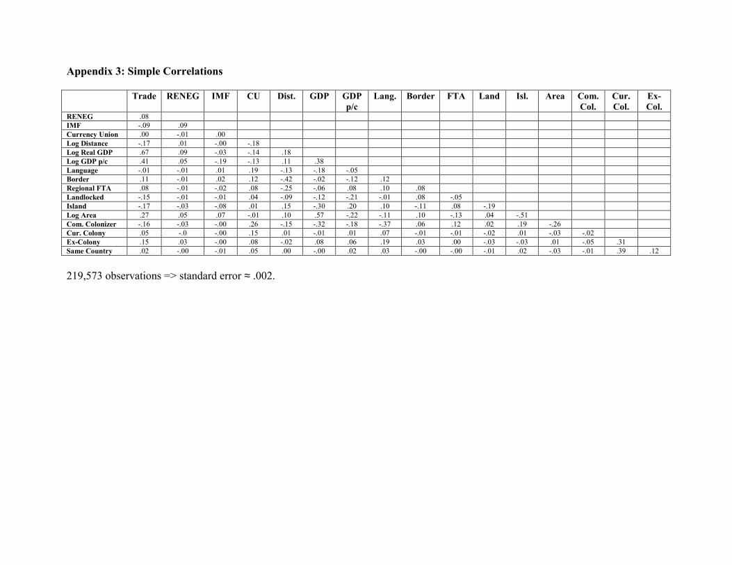
Appendix 3: Simple Correlations

Trade RENEG IMF CU Dist. GDP GDP p/c

Lang. Border FTA Land Isl. Area Com. Col.

Cur. Col.

Ex-Col.

RENEG .08 IMF -.09 .09 Currency Union .00 -.01 .00 Log Distance -.17 .01 -.00 -.18 Log Real GDP .67 .09 -.03 -.14 .18 Log GDP p/c .41 .05 -.19 -.13 .11 .38 Language -.01 -.01 .01 .19 -.13 -.18 -.05 Border .11 -.01 .02 .12 -.42 -.02 -.12 .12 Regional FTA .08 -.01 -.02 .08 -.25 -.06 .08 .10 .08 Landlocked -.15 -.01 -.01 .04 -.09 -.12 -.21 -.01 .08 -.05 Island -.17 -.03 -.08 .01 .15 -.30 .20 .10 -.11 .08 -.19 Log Area .27 .05 .07 -.01 .10 .57 -.22 -.11 .10 -.13 .04 -.51 Com. Colonizer -.16 -.03 -.00 .26 -.15 -.32 -.18 -.37 .06 .12 .02 .19 -.26 Cur. Colony .05 -.0 -.00 .15 .01 -.01 .01 .07 -.01 -.01 -.02 .01 -.03 -.02 Ex-Colony .15 .03 -.00 .08 -.02 .08 .06 .19 .03 .00 -.03 -.03 .01 -.05 .31 Same Country .02 -.00 -.01 .05 .00 -.00 .02 .03 -.00 -.00 -.01 .02 -.03 -.01 .39 .12

219,573 observations => standard error ≈ .002.

References

Babbel, David F. (1996) “Insuring Sovereign Debt against Default, with an annotated bibliography on external debt capacity by Stefano Bertozzi” World Bank Discussion Papers. Bulow, Jeremy and Kenneth Rogoff (1989a) “A Constant Recontracting Model of Sovereign Debt” Journal of Political Economy 97-1, 155-178. Bulow, Jeremy and Kenneth Rogoff (1989b) “Sovereign Debt: Is to Forgive to Forget?” American Economic Review 79-1, 44-50. Cohen, Daniel (1991) Private Lending to Sovereign States (Cambridge: MIT Press). Cole, Harold L. and Patrick J. Kehoe (1997) “Reviving Reputation Models of International Debt” Federal Reserve Bank of Minneapolis Quarterly Review 21-1, 21-30. Dooley, Michael P. (2000) “Can Output Losses Following International Financial Crises be Avoided?” NBER WP 7531. Eaton, Jonathan and Raquel Fernandez (1995) “Sovereign Debt” in The Handbook of International Economics vol. III (edited by G. Grossman and K. Rogoff), 1995, Amsterdam: North-Holland. Eaton, Jonathan, Mark Gersovitz and Joseph Stiglitz (1986) “The Pure Theory of Country Risk” European Economic Review 30, 481-513. Eichengreen, Barry and Richard Portes (1995) Crisis? What Crisis, London: CEPR. Fudenberg, Drew, David Levine and Eric Maskin (1994) “The Folk Theorem with Imperfect Public Information” Econometrica 62, 997-1040. Fudenberg, Drew, and Eric Maskin (1986) “The Folk Theorem for Repeated Games with Discounting and Incomplete Information” Econometrica 54, 533-554. Glick, Reuven and Andrew K. Rose (2002) “Does a Currency Union affect Trade? The Time-Series Evidence” forthcoming European Economic Review. Global Development Finance 2001. Green, Edward, and Robert Porter (1984) “Noncooperative Collusion under Imperfect Price Information” Econometrica 52, 87-100. Hufbauer, Gary Clyde (1998) “Sanctions-Happy USA” International Economics Policy Briefs 98-4. Kaletsky, Anatole (1985) The Costs of Default (New York: Priority Press).

1

Lindert, Peter H. and Peter J. Morton (1989) “How Sovereign Debt has Worked” in (Sachs, ed.) Developing Country Debt and the World Economy (Chicago: University Press). Obstfeld, Maurice and Kenneth Rogoff (1996) Foundations of International Macroeconomics (Cambridge: MIT Press). Rogoff (1999) “International Institutions for Reducing Global Financial Instability” Journal of Economic Perspectives 1304, 21-42. Schott, Jeffrey J. (1998) “US Economic Sanctions: Good Intentions, Bad Execution” http://www.iie.com/papers/schott0698.htm Sevigny, David (1990) The Paris Club: An Inside View, Ottawa: North-South Institute.

2

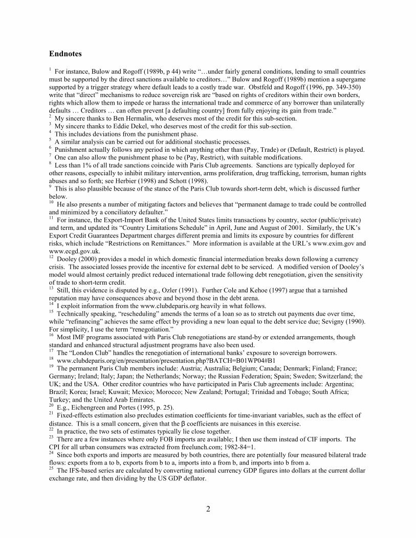
Endnotes 1 For instance, Bulow and Rogoff (1989b, p 44) write “…under fairly general conditions, lending to small countries must be supported by the direct sanctions available to creditors…” Bulow and Rogoff (1989b) mention a supergame supported by a trigger strategy where default leads to a costly trade war. Obstfeld and Rogoff (1996, pp. 349-350) write that “direct” mechanisms to reduce sovereign risk are “based on rights of creditors within their own borders, rights which allow them to impede or harass the international trade and commerce of any borrower than unilaterally defaults … Creditors … can often prevent [a defaulting country] from fully enjoying its gain from trade.” 2 My sincere thanks to Ben Hermalin, who deserves most of the credit for this sub-section. 3 My sincere thanks to Eddie Dekel, who deserves most of the credit for this sub-section. 4 This includes deviations from the punishment phase. 5 A similar analysis can be carried out for additional stochastic processes. 6 Punishment actually follows any period in which anything other than (Pay, Trade) or (Default, Restrict) is played. 7 One can also allow the punishment phase to be (Pay, Restrict), with suitable modifications. 8 Less than 1% of all trade sanctions coincide with Paris Club agreements. Sanctions are typically deployed for other reasons, especially to inhibit military intervention, arms proliferation, drug trafficking, terrorism, human rights abuses and so forth; see Herbier (1998) and Schott (1998). 9 This is also plausible because of the stance of the Paris Club towards short-term debt, which is discussed further below. 10 He also presents a number of mitigating factors and believes that “permanent damage to trade could be controlled and minimized by a conciliatory defaulter.” 11 For instance, the Export-Import Bank of the United States limits transactions by country, sector (public/private) and term, and updated its “Country Limitations Schedule” in April, June and August of 2001. Similarly, the UK’s Export Credit Guarantees Department charges different premia and limits its exposure by countries for different risks, which include “Restrictions on Remittances.” More information is available at the URL’s www.exim.gov and www.ecgd.gov.uk. 12 Dooley (2000) provides a model in which domestic financial intermediation breaks down following a currency crisis. The associated losses provide the incentive for external debt to be serviced. A modified version of Dooley’s model would almost certainly predict reduced international trade following debt renegotiation, given the sensitivity of trade to short-term credit. 13 Still, this evidence is disputed by e.g., Ozler (1991). Further Cole and Kehoe (1997) argue that a tarnished reputation may have consequences above and beyond those in the debt arena. 14 I exploit information from the www.clubdeparis.org heavily in what follows. 15 Technically speaking, “rescheduling” amends the terms of a loan so as to stretch out payments due over time, while “refinancing” achieves the same effect by providing a new loan equal to the debt service due; Sevigny (1990). For simplicity, I use the term “renegotiation.” 16 Most IMF programs associated with Paris Club renegotiations are stand-by or extended arrangements, though standard and enhanced structural adjustment programs have also been used. 17 The “London Club” handles the renegotiation of international banks’ exposure to sovereign borrowers. 18 www.clubdeparis.org/en/presentation/presentation.php?BATCH=B01WP04#B1 19 The permanent Paris Club members include: Austria; Australia; Belgium; Canada; Denmark; Finland; France; Germany; Ireland; Italy; Japan; the Netherlands; Norway; the Russian Federation; Spain; Sweden; Switzerland; the UK; and the USA. Other creditor countries who have participated in Paris Club agreements include: Argentina; Brazil; Korea; Israel; Kuwait; Mexico; Morocco; New Zealand; Portugal; Trinidad and Tobago; South Africa; Turkey; and the United Arab Emirates. 20 E.g., Eichengreen and Portes (1995, p. 25). 21 Fixed-effects estimation also precludes estimation coefficients for time-invariant variables, such as the effect of distance. This is a small concern, given that the β coefficients are nuisances in this exercise. 22 In practice, the two sets of estimates typically lie close together. 23 There are a few instances where only FOB imports are available; I then use them instead of CIF imports. The CPI for all urban consumers was extracted from freelunch.com; 1982-84=1. 24 Since both exports and imports are measured by both countries, there are potentially four measured bilateral trade flows: exports from a to b, exports from b to a, imports into a from b, and imports into b from a. 25 The IFS-based series are calculated by converting national currency GDP figures into dollars at the current dollar exchange rate, and then dividing by the US GDP deflator.

3

26 The website is: http://www.odci.gov/cia/publications/factbook. 27 All FTAs are treated as being equal for simplicity. 28 A few multilateral official debt renegotiations have been conducted outside the Paris Club forum, e.g., by the OECD, creditor groups, or special task forces. Information on these has been included from records of the Paris Club and Global Development Finance. 29 Over 93% of all Paris Club agreements are preceded by an IMF program within five years. 30 There were also 56 uses of the Extended Fund Facility (intended to address more protracted issues), 33 of the Structural Adjustment Facility and 70 of its successor Enhanced Structural Adjustment Facilities, the latter both intended for low-income countries. Both the Supplemental Reserve Facility and the Contingent Credit Line began in 1997, while the concessional Poverty Reduction and Growth Facility began only in 1999; these are ignored in this paper. 31 Data on IMF programs are available from the IMF’s Annual Report; I thank Eduardo Borensztein and Jeromin Zettlemeyer for assistance in obtaining data on IMF programs. 32 Thus, the fixed-effect estimation of renegotiations between one and five years ago is derived by adding .09 and -.23, while the effect of renegotiation between six and ten years ago is simply -.23. 33 For the Tobit estimation, small values of trade (less than $1,000) are set to zero. 34 While the linear panel fixed- or random-effects estimates of Table 1 can be computed in a few seconds on a Pentium III, the results of Table 3 require over 40 hours to converge. 35 I have also used different sets of IVs with similar, though usually weaker results. 36 Indeed, there may even be a net positive effect, though the data speak quietly on this issue. 37 The results are always sensible (bigger renegotiations tend to dampen trade more, while countries that were recently rescheduled or have frequently had their debts rescheduled tend to trade less), and sometimes significant, especially with the GLS estimator.