Dr. John Mellor-Crummey

Department of Computer ScienceRice University

johnmc@cs.rice.edu

One-Factor Designs

COMP 528 Lecture 15 15 March 2005

2

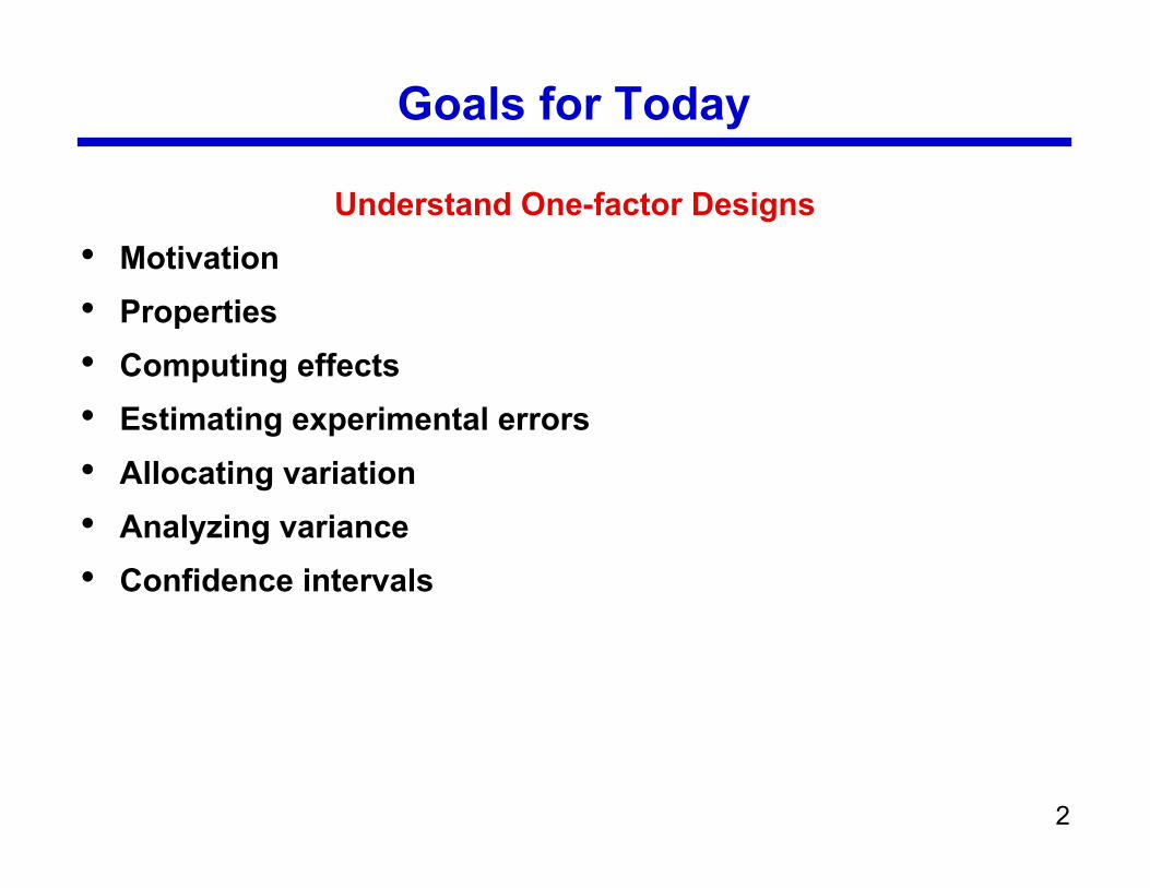
Goals for Today

Understand One-factor Designs• Motivation• Properties• Computing effects• Estimating experimental errors• Allocating variation• Analyzing variance• Confidence intervals

3

One-factor Designs

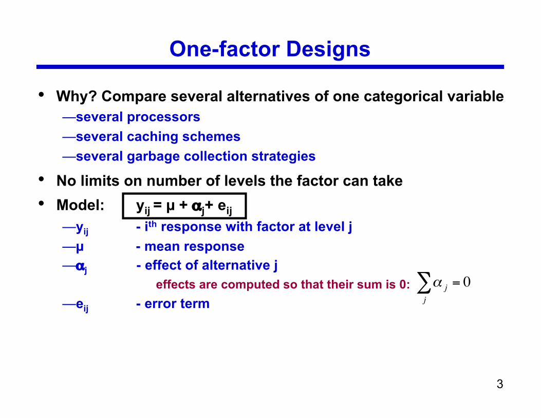
• Why? Compare several alternatives of one categorical variable—several processors—several caching schemes—several garbage collection strategies

• No limits on number of levels the factor can take• Model: yij = µ + αj+ eij

—yij - ith response with factor at level j—µ - mean response—αj - effect of alternative j

effects are computed so that their sum is 0:—eij - error term

!

" j

j

# = 0

4

Computing Effects for a One-factor Design

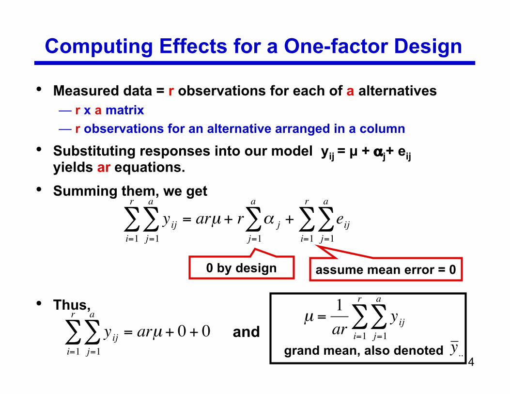
• Measured data = r observations for each of a alternatives— r x a matrix— r observations for an alternative arranged in a column

• Substituting responses into our model yij = µ + αj+ eijyields ar equations.

• Summing them, we get

• Thus,!

yijj=1

a

"i=1

r

" = arµ + r # j

j=1

a

" + eijj=1

a

"i=1

r

"

!

yijj=1

a

"i=1

r

" = arµ + 0 + 0

0 by design assume mean error = 0

and

!

µ =1

aryij

j=1

a

"i=1

r

"

grand mean, also denoted

!

y ..

5

Mean Effect for an Alternative

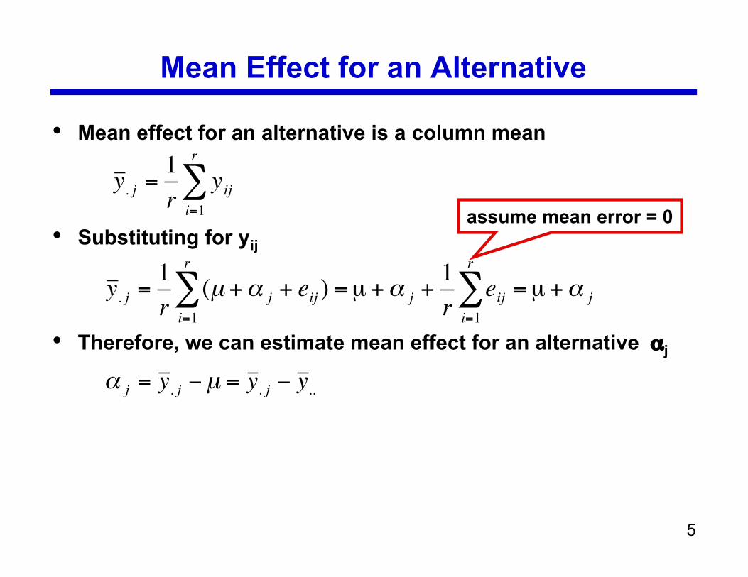
• Mean effect for an alternative is a column mean

• Substituting for yij

• Therefore, we can estimate mean effect for an alternative αj

!

" j = y . j #µ = y

. j # y ..

!

y . j =

1

ryij

i=1

r

"

!

y . j =

1

r(µ +" j + eij )

i=1

r

# = µ +" j +1

reij

i=1

r

# = µ +" j

assume mean error = 0

6

Tabular Computation of Mean Effect

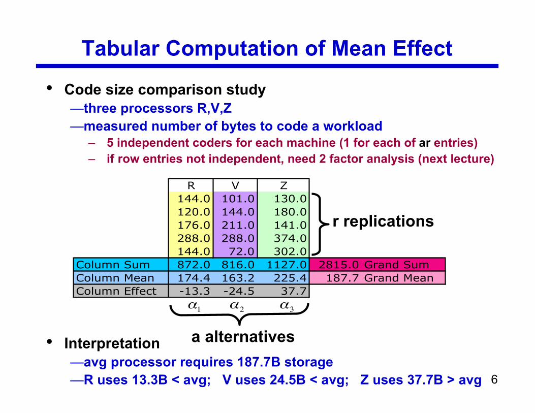
• Code size comparison study—three processors R,V,Z—measured number of bytes to code a workload

– 5 independent coders for each machine (1 for each of ar entries)– if row entries not independent, need 2 factor analysis (next lecture)

• Interpretation—avg processor requires 187.7B storage—R uses 13.3B < avg; V uses 24.5B < avg; Z uses 37.7B > avg

R V Z

144.0 101.0 130.0

120.0 144.0 180.0

176.0 211.0 141.0

288.0 288.0 374.0

144.0 72.0 302.0

Column Sum 872.0 816.0 1127.0 2815.0 Grand Sum

Column Mean 174.4 163.2 225.4 187.7 Grand Mean

Column Effect -13.3 -24.5 37.7

!

"1

!

"2

!

"3

r replications

a alternatives

7

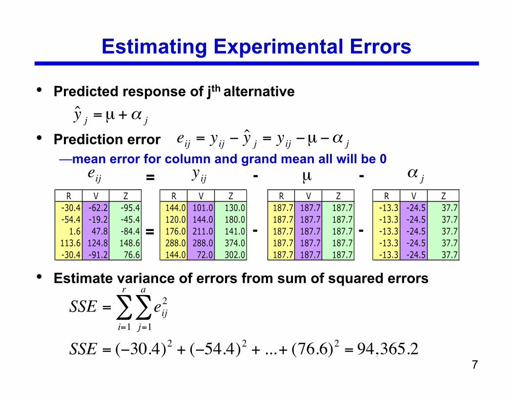
Estimating Experimental Errors

• Predicted response of jth alternative

• Prediction error—mean error for column and grand mean all will be 0

• Estimate variance of errors from sum of squared errors

!

ˆ y j = µ +" j

!

eij = yij " ˆ y j = yij "µ "# j

!

SSE = eij2

j=1

a

"i=1

r

"

R V Z

144.0 101.0 130.0

120.0 144.0 180.0

176.0 211.0 141.0

288.0 288.0 374.0

144.0 72.0 302.0

R V Z

187.7 187.7 187.7

187.7 187.7 187.7

187.7 187.7 187.7

187.7 187.7 187.7

187.7 187.7 187.7

R V Z

-13.3 -24.5 37.7

-13.3 -24.5 37.7

-13.3 -24.5 37.7

-13.3 -24.5 37.7

-13.3 -24.5 37.7

R V Z

-30.4 -62.2 -95.4

-54.4 -19.2 -45.4

1.6 47.8 -84.4

113.6 124.8 148.6

-30.4 -91.2 76.6

= - -!

eij

!

yij

!

µ

!

" j= - -

!

SSE = ("30.4)2

+ ("54.4)2

+ ...+ (76.6)2

= 94,365.2

8

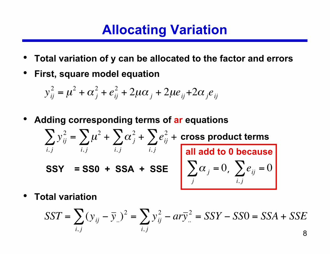
Allocating Variation

• Total variation of y can be allocated to the factor and errors• First, square model equation

• Adding corresponding terms of ar equations

• Total variation!

yij2

i, j

" = µ2

i, j

" + # j

2

i, j

" + eij2

i, j

" +!

yij2 = µ2 +" j

2 + eij2 + 2µ" j + 2µeij+2" jeij

cross product termsall add to 0 because

!

" j

j

# = 0

!

eiji, j

" = 0,SSY = SS0 + SSA + SSE

!

SST = (yij " y ..)2

i, j

# = yij

2 " ary ..

2

i, j

# = SSY " SS0 = SSA + SSE

9

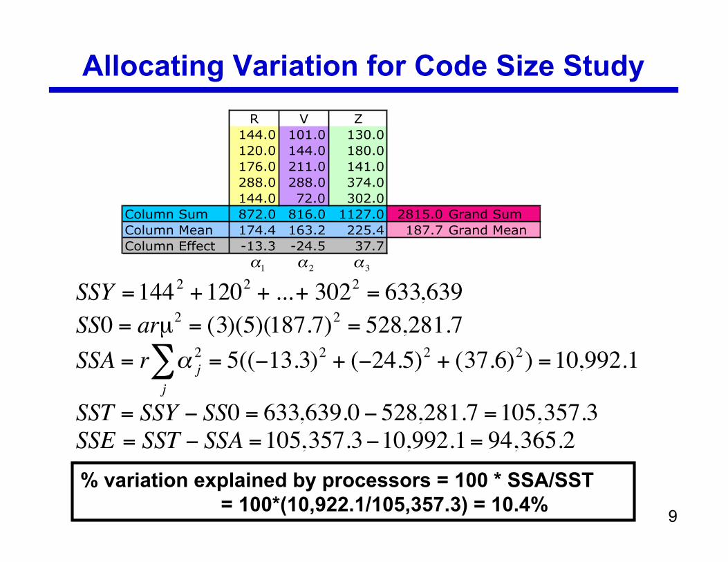
Allocating Variation for Code Size Study

% variation explained by processors = 100 * SSA/SST = 100*(10,922.1/105,357.3) = 10.4%

R V Z

144.0 101.0 130.0

120.0 144.0 180.0

176.0 211.0 141.0

288.0 288.0 374.0

144.0 72.0 302.0

Column Sum 872.0 816.0 1127.0 2815.0 Grand Sum

Column Mean 174.4 163.2 225.4 187.7 Grand Mean

Column Effect -13.3 -24.5 37.7

!

"1

!

"2

!

"3

!

SSY =1442

+1202

+ ...+ 3022

= 633,639

!

SST = SSY " SS0 = 633,639.0 " 528,281.7 =105,357.3

!

SSE = SST " SSA =105,357.3"10,992.1= 94,365.2

!

SSA = r " j

2

j

# = 5(($13.3)2 + ($24.5)2 + (37.6)2) =10,992.1

!

SS0 = arµ2 = (3)(5)(187.7)2 = 528,281.7

10

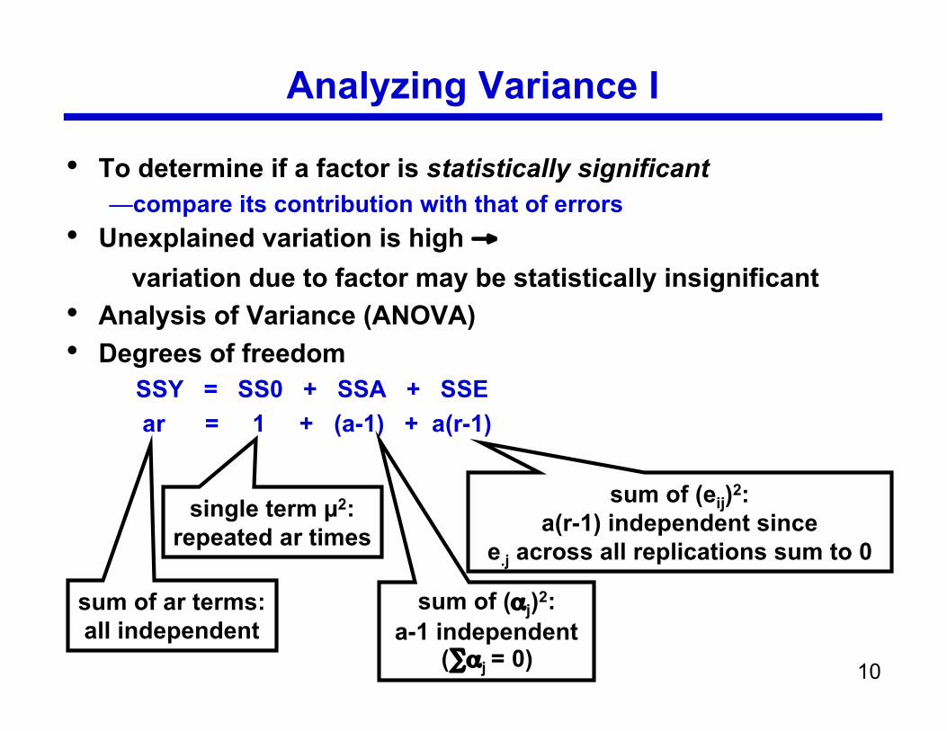
Analyzing Variance I

• To determine if a factor is statistically significant—compare its contribution with that of errors

• Unexplained variation is high → variation due to factor may be statistically insignificant• Analysis of Variance (ANOVA)• Degrees of freedom

SSY = SS0 + SSA + SSE ar = 1 + (a-1) + a(r-1)

sum of ar terms:all independent

single term µ2:repeated ar times

sum of (αj)2:a-1 independent

(∑αj = 0)

sum of (eij)2:a(r-1) independent since

e.j across all replications sum to 0

11

Analyzing Variance II

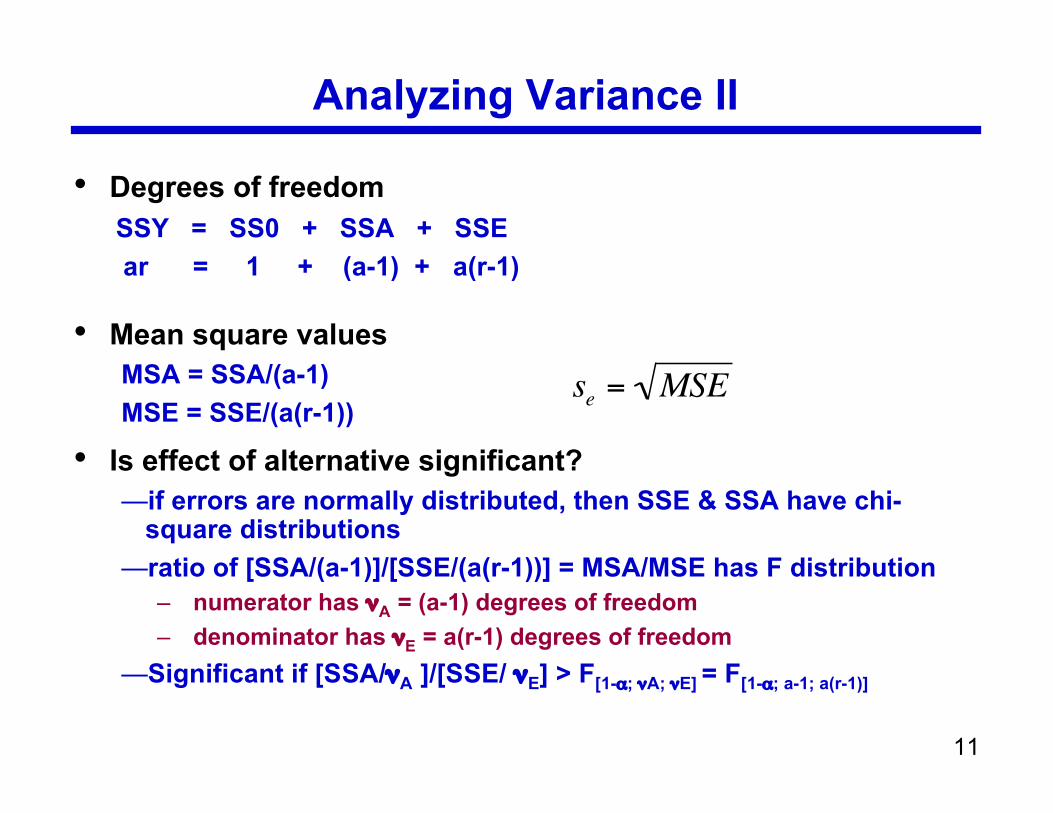
• Degrees of freedom

• Mean square valuesMSA = SSA/(a-1)MSE = SSE/(a(r-1))

• Is effect of alternative significant?—if errors are normally distributed, then SSE & SSA have chi-

square distributions—ratio of [SSA/(a-1)]/[SSE/(a(r-1))] = MSA/MSE has F distribution

– numerator has νA = (a-1) degrees of freedom– denominator has νE = a(r-1) degrees of freedom

—Significant if [SSA/νA ]/[SSE/ νE] > F[1-α; νA; νE] = F[1-α; a-1; a(r-1)]

SSY = SS0 + SSA + SSE ar = 1 + (a-1) + a(r-1)

!

se

= MSE

12

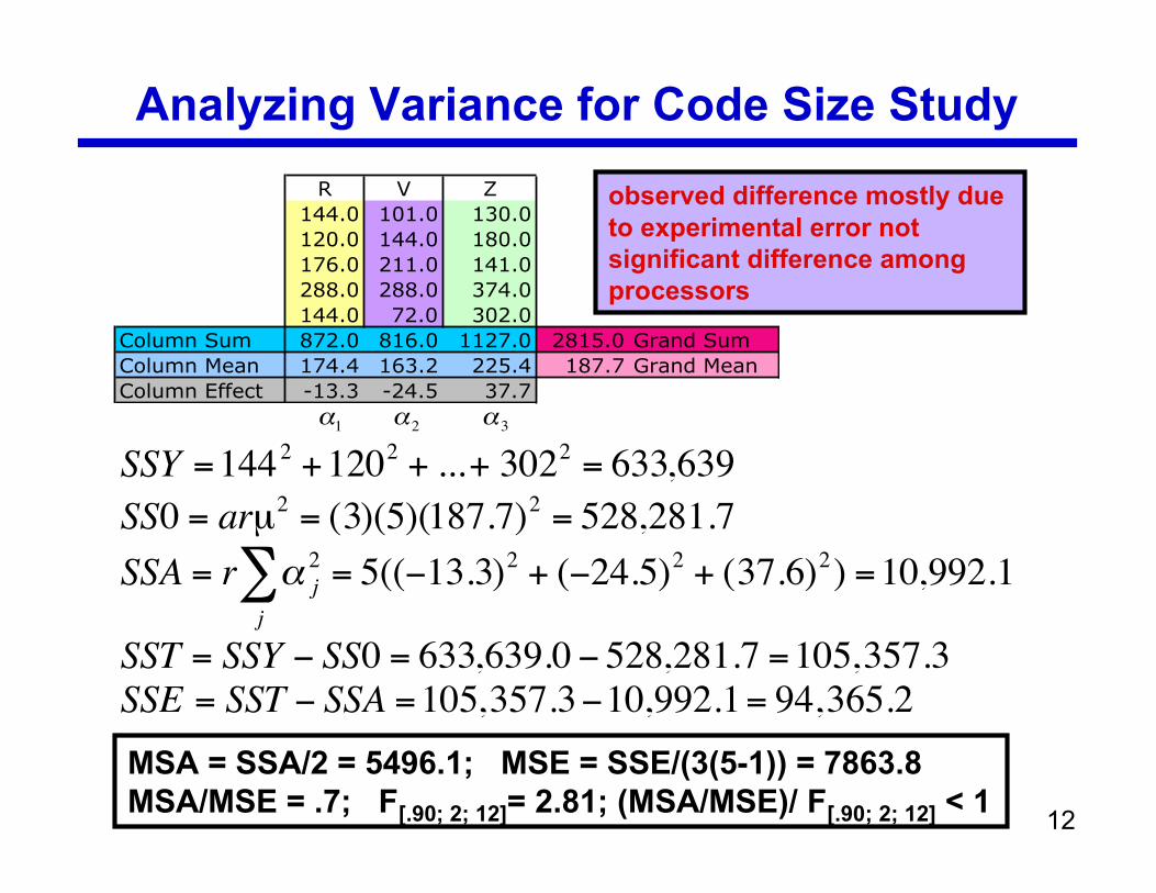
Analyzing Variance for Code Size Study

MSA = SSA/2 = 5496.1; MSE = SSE/(3(5-1)) = 7863.8MSA/MSE = .7; F[.90; 2; 12]= 2.81; (MSA/MSE)/ F[.90; 2; 12] < 1

R V Z

144.0 101.0 130.0

120.0 144.0 180.0

176.0 211.0 141.0

288.0 288.0 374.0

144.0 72.0 302.0

Column Sum 872.0 816.0 1127.0 2815.0 Grand Sum

Column Mean 174.4 163.2 225.4 187.7 Grand Mean

Column Effect -13.3 -24.5 37.7

!

"1

!

"2

!

"3

!

SSY =1442

+1202

+ ...+ 3022

= 633,639

!

SST = SSY " SS0 = 633,639.0 " 528,281.7 =105,357.3

!

SSE = SST " SSA =105,357.3"10,992.1= 94,365.2

!

SSA = r " j

2

j

# = 5(($13.3)2 + ($24.5)2 + (37.6)2) =10,992.1

!

SS0 = arµ2 = (3)(5)(187.7)2 = 528,281.7

observed difference mostly due to experimental error not significant difference among processors

13

Assumptions of One-factor Experiments

• Effects of various factors are additive• Errors are additive• Errors are independent of factor levels• Errors are normally distributed• Errors have the same variance for all factor levels

14

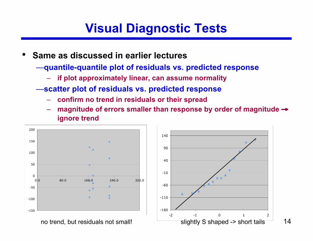
Visual Diagnostic Tests

• Same as discussed in earlier lectures—quantile-quantile plot of residuals vs. predicted response

– if plot approximately linear, can assume normality—scatter plot of residuals vs. predicted response

– confirm no trend in residuals or their spread– magnitude of errors smaller than response by order of magnitude →

ignore trend

no trend, but residuals not small! slightly S shaped -> short tails

15

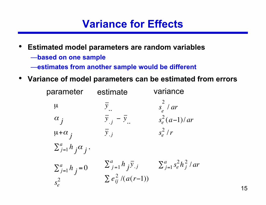
Variance for Effects

• Estimated model parameters are random variables—based on one sample—estimates from another sample would be different

• Variance of model parameters can be estimated from errors

!

µ

" j

µ+"j

hj"j,j=1

a#

hj

= 0j=1a#

se2

!

y ..

y . j" y ..

y . j

hjy . jj =1

a#

eij2/(a(r"1))#

!

se

2

/ ar

se2(a"1)/ ar

se2/ r

se2h j2/ arj=1

a#

parameter estimate variance

16

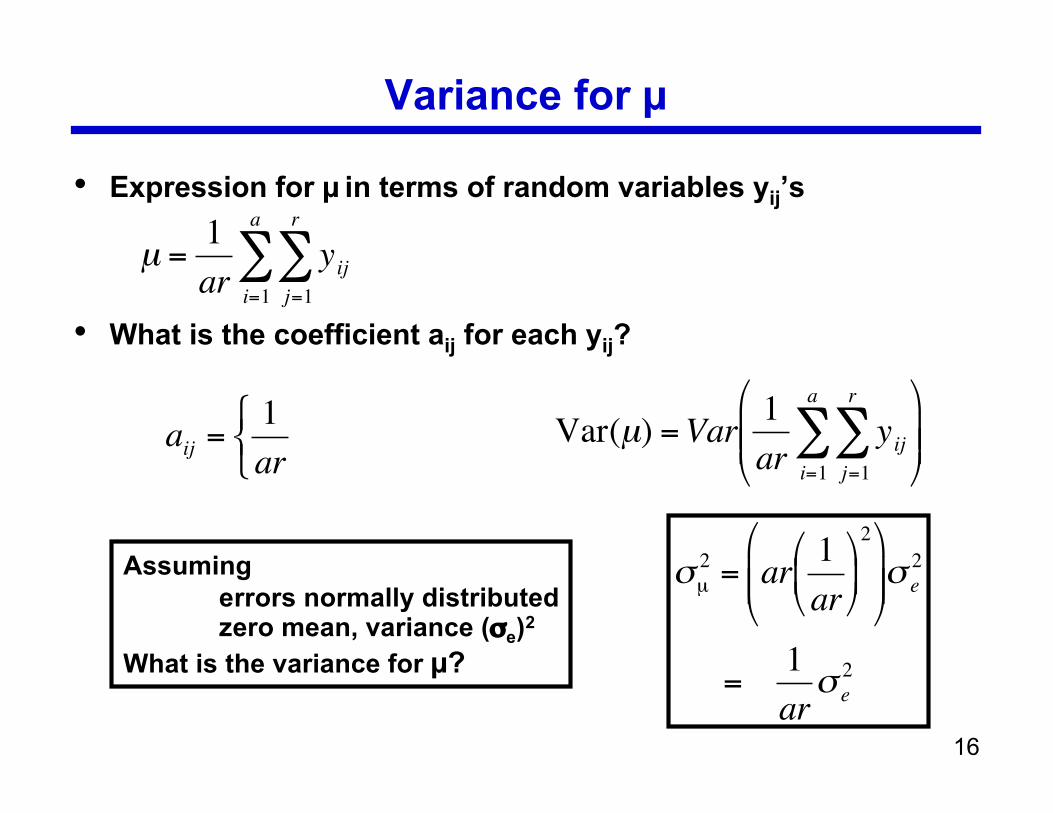
Variance for µ

• Expression for µ in terms of random variables yij’s

• What is the coefficient aij for each yij?

!

µ =1

aryij

j=1

r

"i=1

a

"

!

aij =1

ar

" # $

Assuming errors normally distributedzero mean, variance (σe)2

What is the variance for µ?

!

"µ

2 = ar1

ar

#

$ %

&

' (

2#

$ % %

&

' ( ( " e

2

=1

ar"e

2

!

Var(µ) =Var1

aryij

j=1

r

"i=1

a

"#

$ % %

&

' ( (

17

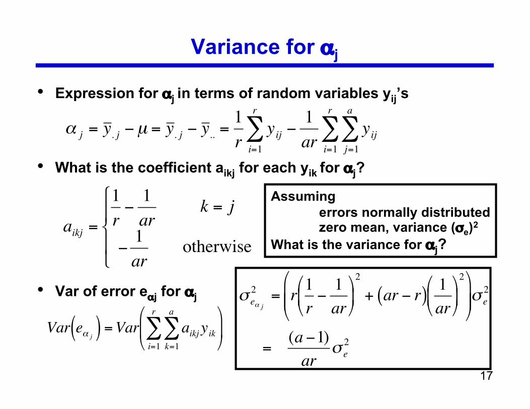
Variance for αj

• Expression for αj in terms of random variables yij’s

• What is the coefficient aikj for each yik for αj?

• Var of error eαj for αj

!

" j = y . j #µ = y

. j # y ..

=1

ryij #

1

aryij

j=1

a

$i=1

r

$i=1

r

$

!

aikj =

1

r"1

ar

"1

ar

k = j

otherwise

#

$ %

& %

!

Var e" j( ) =Var aikj yik

k=1

a

#i=1

r

#$

% &

'

( )

Assuming errors normally distributedzero mean, variance (σe)2

What is the variance for αj?

!

" e# j

2 = r1

r$1

ar

%

& '

(

) *

2

+ ar $ r( )1

ar

%

& '

(

) *

2%

& ' '

(

) * * " e

2

=(a $1)

ar" e

2

18

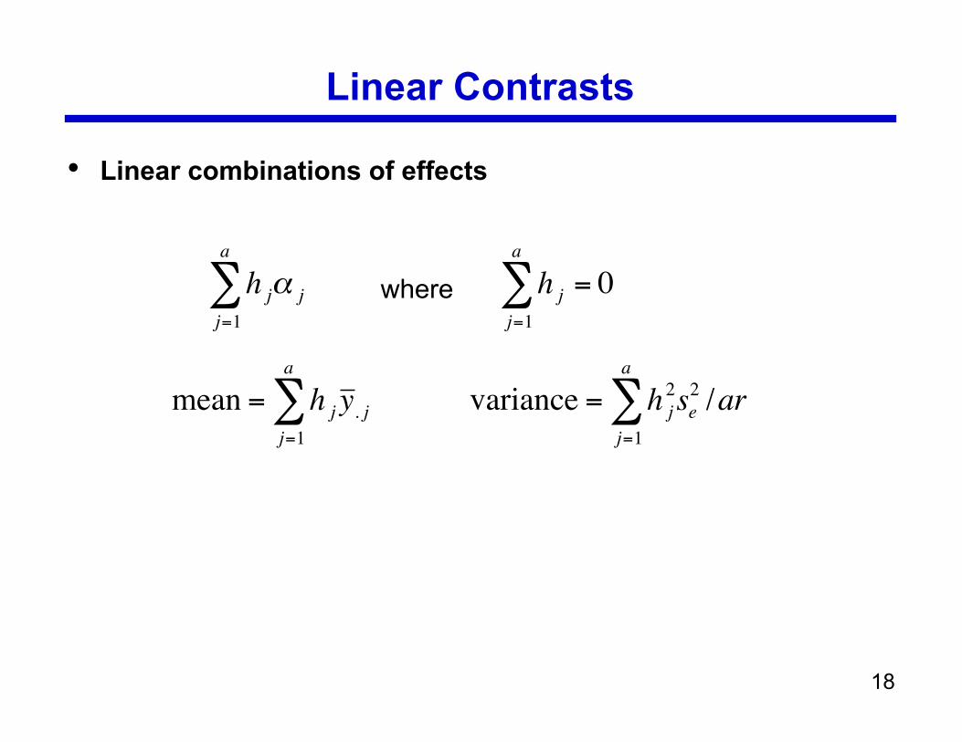
Linear Contrasts

• Linear combinations of effects

!

h j" j

j=1

a

# where

!

h j = 0j=1

a

"

!

mean = h j y . j

j=1

a

"

!

variance = h j

2se2/ar

j=1

a

"

19

Confidence Intervals for Effects

• Compute confidence intervals with t values read out of tableat a(r-1) degrees of freedom (DOF of errors)