ONE-DIMENSIONAL, ONE-PHASE RESERVOIR SIMULATION …kleppe/TPG4160/note4.pdf · TPG4160 Reservoir Simulation 2017 Lecture note 4 Norwegian University of Science and Technology Professor

TPG4160 Reservoir Simulation 2017 Lecture note 4

Norwegian University of Science and Technology Professor Jon Kleppe Department of Petroleum Engineering and Applied Geophysics 12.1.17

page 1 of 9

ONE-DIMENSIONAL, ONE-PHASE RESERVOIR SIMULATION Fluid systems The term single phase applies to any system with only one phase present in the reservoir. In some cases it may also apply where two phases are present in the reservoir, if one of the phases is immobile, and no mass exchange takes place between the fluids. This is normally the case where immobile water is present with oil or with gas in the reservoir. By regarding the immobile water as a fixed part of the pores, it can be accounted for by reducing porosity and modifying rock compressibility correspondingly. Normally, in one phase reservoir simulation we would deal with one of the following fluid systems:

1. One phase gas 2. One phase water 3. One phase oil

Before proceeding to the flow equations, we will briefly define the fluid models for these three systems. One phase gas The gas must be single phase in the reservoir, which means that crossing of the dew point line is not permitted in order to avoid condensate fallout in the pores. Fluid behavior is governed by our Black Oil fluid model, so that

ρg =ρgs

Bg= constant

Bg.

One phase water One phase water, which strictly speaking means that the reservoir pressure is higher than the saturation pressure of the water in case gas is dissolved in it, has a density described by:

ρw =ρws

Bw= constant

Bw.

One phase oil In order for the oil to be single phase in the reservoir, it must be undersaturated, which means that the reservoir pressure is higher than the bubble point pressure. In the Black Oil fluid model, oil density is described by:

ρo =ρoS + ρgSRso

Bo.

For undersaturated oil, is constant, and the oil density may be written:

ρo =constantBo

.

General form Thus, for all three fluid systems, the one phase density may be expressed as:



page 2 of 9

ρ = constantB

,

which is the model we are going to use for the fluid description in the following single phase flow equations. Partial differential form of single phase flow equation We have previously derived the continuity equation for a one phase, one-dimensional system of constant cross-sectional area to be:

− ∂∂ x

ρu( ) = ∂∂ t

φρ( ) .

The conservation of momentum for low velocity flow in porous materials is assumed to be described by the semi-empirical Darcy's equation, which for one dimensional, horizontal flow is:

u = − kµ∂P∂ x

.

Using the fluid model defined above:

ρ = constantB

,

and substituting the Darcy's equation and the fluid equation into the continuity equation, and including a source/sink term, we obtain the partial differential equation that describes single phase flow in a one dimensional porous medium:

∂∂ x

kµB

∂P∂x

⎛⎝⎜

⎞⎠⎟− ′q = ∂

∂ tφB

⎛⎝⎜

⎞⎠⎟

The left hand side of the equation describes fluid flow in the reservoir, and injection/production, while the right hand side represent storage (compressibilities of rock and fluid). In order to bring the right hand side of the equation on a form with pressure as a primary variable, we will rearrange the term before proceeding to the numerical solution. Chain rule differentiation yields:

∂∂ t

φB

⎛⎝⎜

⎞⎠⎟ =

1B∂φ∂t

+φ ∂(1 / B)∂t

We will now make use of the compressibility definition for porosity's dependency of pressure at constant temperature:

cr =1φdφdP

,

or

dφdP

= φcr ,

and the fluid model above:



page 3 of 9

ρ = constantB

,

which implies that: B = f (P) . The right hand side may then be written:

∂∂ t

φB

⎛⎝⎜

⎞⎠⎟ =

1B∂φ∂t

+φ ∂(1 / B)∂t

= 1BdφdP

∂P∂t

+φ d(1 / B)dP

∂P∂t

=φcrB

∂P∂t

+φ d(1 / B)dP

∂P∂t

Thus, the flow equation becomes:

∂∂ x

kµB

∂P∂x

⎛⎝⎜

⎞⎠⎟− ′q = φ cr

B+ d(1 / B)

dP⎡⎣⎢

⎤⎦⎥∂P∂t

Recall that the fluid compressibility may be defined in terms of the formation volume factor as:

cf = Bd(1 / B)dP

.

Then, an alternative form of the flow equation is:

∂∂ x

kµB

∂P∂x

⎛⎝⎜

⎞⎠⎟− ′q = φ

Bcr + cf⎡⎣ ⎤⎦

∂P∂t

= φcTB

∂P∂t

However, normally it is more convenient to use the first form, since fluid compressibility not necessarily is constant, and since formation volume factor vs. pressure data is standard input to reservoir simulators. Difference form of the flow equation We will now use the discretization formulas derived previously to transform our partial differential equation to difference form. For convenience, we will now drop the time index for unknown pressures, so that if no time index is specified, t + Δt is implied. Left side term The single phase flow term,

∂∂ x

kµB

∂P∂x

⎛⎝⎜

⎞⎠⎟

is of the form:

∂∂ x

f (x)∂P∂ x

⎡⎣⎢

⎤⎦⎥

,

which we previously derived the following approximation for:



page 4 of 9

∂∂ x

f (x)∂P∂ x

⎡⎣⎢

⎤⎦⎥i=2 f (x)i+1/2

(Pi+1 − Pi )(Δxi+1 + Δxi )

− 2 f (x)i−1/2(Pi − Pi−1)(Δxi + Δxi−1)

Δxi+O(Δx) .

Thus, in terms of the actual flow equation above, we have:

∂∂ x

kµB

∂P∂ x

⎛⎝⎜

⎞⎠⎟ i=2 k

µB⎛⎝⎜

⎞⎠⎟ i+1/2

(Pi+1 − Pi )(Δxi+1 + Δxi )

− 2 kµB

⎛⎝⎜

⎞⎠⎟ i−1/2

(Pi − Pi−1)(Δxi + Δxi−1)

Δxi+O(Δx) .

We shall now define transmissibility as being the coefficient in front of the pressure difference appearing in the approximation above: Transmissibility in plus direction

Txi+1/2 =2

Δxi (Δxi+1 + Δxi )kµB

⎛⎝⎜

⎞⎠⎟ i+1/2

Transmissibility in minus direction

Txi−1/2 =2

Δxi (Δxi−1 + Δxi )kµB

⎛⎝⎜

⎞⎠⎟ i−1/2

.

Then, the difference form of the flow term in the partial differential equation becomes:

∂∂ x

kµB

∂P∂ x

⎛⎝⎜

⎞⎠⎟ i

≈ Txi+1/2 (Pi+1 − Pi )+Txi−1/2 (Pi−1 − Pi ) .

Using Txi+1/2 as example, the transmissibility consists of three groups of parameters:

2

Δxi (Δxi+1 + Δxi )= constant ,

ki+1/2 = k = f (x),

1µB

⎛⎝⎜

⎞⎠⎟ i+1/2

= 1µB

⎛⎝⎜

⎞⎠⎟= f (P).

We therefore need to determine the forms of the two latter groups before proceeding to the numerical solution. Starting with Darcy's equation:

q = − kAµB

∂P∂x

.

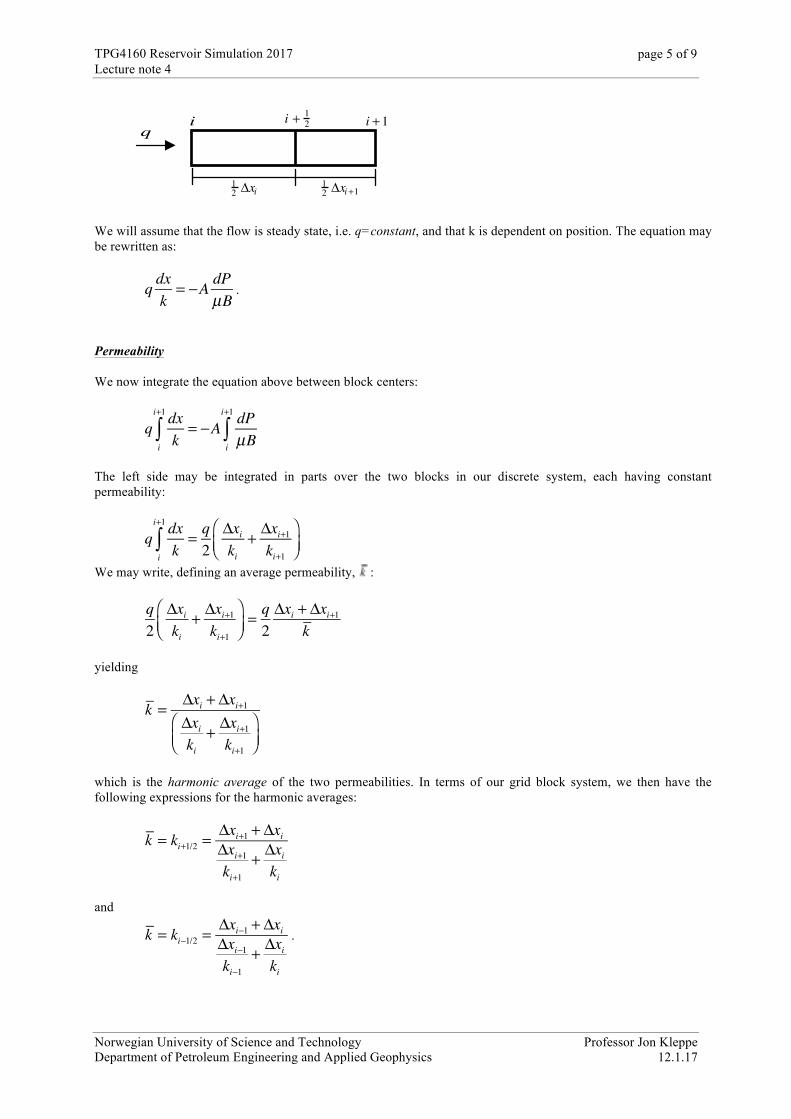
For flow between two grid blocks:



page 5 of 9

We will assume that the flow is steady state, i.e. q=constant, and that k is dependent on position. The equation may be rewritten as:

q dxk

= −A dPµB

.

Permeability We now integrate the equation above between block centers:

q dxki

i+1

∫ = −A dPµBi

i+1

∫

The left side may be integrated in parts over the two blocks in our discrete system, each having constant permeability:

q dxki

i+1

∫ = q2

Δxiki

+ Δxi+1ki+1

⎛⎝⎜

⎞⎠⎟

We may write, defining an average permeability, :

q2

Δxiki

+ Δxi+1ki+1

⎛⎝⎜

⎞⎠⎟= q2Δxi + Δxi+1

k

yielding

k = Δxi + Δxi+1Δxiki

+ Δxi+1ki+1

⎛⎝⎜

⎞⎠⎟

which is the harmonic average of the two permeabilities. In terms of our grid block system, we then have the following expressions for the harmonic averages:

k = ki+1/2 =Δxi+1 + ΔxiΔxi+1ki+1

+ Δxiki

and

k = ki−1/2 =Δxi−1 + ΔxiΔxi−1ki−1

+ Δxiki

.

i + 12 i + 1i

12 Δxi

12 Δxi+1

q



page 6 of 9

Fluid mobility term We want to integrate the right hand side:

−A dPµBi

i+1

∫

Replacing the fluid parameters by mobility λ = 1µB

, and letting be a weak function of pressure, and assuming

the pressure gradient between the block centers to be constant, we find that the weighted average of the blocks' mobility terms is representative of the average. First, we will define the fluid mobility term as. Then, the average mobility terms are:

λi+1/2 =Δxi+1λi+1 + Δxiλi( )

Δxi+1 + Δxi( )

and

λi−1/2 =Δxi−1λi−1 + Δxiλi( )

Δxi−1 + Δxi( ) .

Right side term The discretization of the right side term

φ crB+ d(1 / B)

dP⎡⎣⎢

⎤⎦⎥∂P∂t

is done by using the backward difference approximation derived previously:

(∂P∂ t)i ≈

Pi − Pit

Δt.

We will now define a storage coefficient as:

Cpi =φiΔt

crB+ d(1 / B)

dP⎡⎣⎢

⎤⎦⎥i

and the right side approximation becomes:

φ crB+ d(1 / B)

dP⎡⎣⎢

⎤⎦⎥∂P∂t

≈Cpi (Pi − Pit )

Thus, the difference form of the single phase flow equation is (for convenience, the approximation sign is hereafter replaced by an equal sign): Txi+1/2 (Pi+1 − Pi )+Txi−1/2 (Pi−1 − Pi )− ′qi = Cpi (Pi − Pi

t ), i = 1,N .



page 7 of 9

Boundary conditions and production/injection terms We have previously discussed the two types of boundary conditions we can assign, the pressure specification (Dirichlet condition) and the rate condition (Neumann condition). For the simple one phase equation that we considered initially, we assumed these to be specified at either the end of the system and derived corresponding approximations of the flow term for these grid blocks. However, in reservoir simulation the boundary conditions normally are no flow boundaries at the end faces of the reservoir, and production/injection wells where either rate or pressure are specified, located in any of the grid blocks. No flow boundaries No flow at the boundaries are assigned by giving the respective transmissibility a zero value at that point. This is the default condition. For our one-dimensional system, this type of condition would for example be applied to the two end blocks so that: Tx1/2 = 0 TxN+1/2 = 0 . Production/injection wells We will now introduce a well term in our difference equation, so that it becomes:

Txi+1/2 (Pi+1 − Pi )+Txi−1/2 (Pi−1 − Pi )− ′qi = Cpi (Pi − Pit ), i = 1,N .

The well rate term will be zero for all blocks that do not have a well in it, and nonzero where there is a well. Since our equation is formulated on a per volume basis, the flow rate must also be on a per volume basis. It is defined as positive for production wells and negative for injection wells. Constant well production rate, Qi

For a constant well rate of at surface conditions, which is the most common well rate specification, the per volume rate becomes:

′qi =Qi

AΔxi.

If the well is specified to have a constant well rate of at reservoir conditions, the per volume rate becomes:

′qi =Qi

BiAΔxi.

Constant well bottom-hole pressure

For a well producing or injecting at a constant bottom hole pressure, Pbhi , the well rate is computed the following equation:

′qi =Qi

AΔxi= WCiλi (Pi − Pbhi )

AΔxi= wciλi (Pi − Pbhi ) ,



page 8 of 9

where WCi is the the well constant, or the productivity or injectivity index of the well, and the same on a per volume basis. The well constant may be specified externally, based on productivity or injectivity tests of the well, or it may be computed from Darcy's equation. If the well is in the middle of the grid block, one may assume radial flow into the well, with block volume as the drainage volume:

WCi =2πkih

ln( rerw)

,

where rw is the wellbore radius, and the drainage radius may theoretically be defined as:

re =ΔyΔxiπ

.

However, in reservoir simulation this formula is normally written as:

re = c ΔyΔxi Where the value c may vary depending on well location inside the grid block. A commonly used formula is the one derived by Peaceman:

re = 0.20 ΔyΔxi For the simple linear case, with a well is at the end of the system, at the left or right faces, the well constant would be computed from the linear Darcy's equation:

WCi =kiA

Δxi / 2.

Solution of the difference equation Now we have a set of N equations with N unknowns, which must be solved simultaneously. In deriving the difference equation we have implicitly assumed that all terms of the equation are evaluated at time . This assumption applies to the coefficients as well as the pressures on the left side of the equation. However, one may question the numerical correctness of this since the approximation of the time derivative on the right hand side then becomes a first order backward difference. If instead the terms were to be evaluated at , the time derivative would become a second order approximation, central in time, and thus a more accurate approximation. Such a formulation is known as a Crank-Nicholson formulation. Since the pressure solution of such a formulation often exhibits oscillatory behavior, it is normally not used in reservoir simulation, and we will therefore not pursue it further here. Since the left and right hand side terms of the equation are at time , the coefficients are functions of the unknown pressure. In the transmissibility terms, both viscosity and formation volume factor are pressure dependent, and in the storage terms the derivative of the inverse formation volume factor depends on pressure. Therefore, an obvious procedure would be to iterate on the pressure solution, letting the coefficients lag one iteration behind and updating them after each iteration until convergence is obtained. However, in single phase flow the pressure dependency of the coefficients is small, and such iteration is normally not necessary. For now we will therefore make the approximation that the transmissibilities and the storage coefficients with sufficient accuracy can be evaluated at the block pressures at the previous time step. The set of equations may be rewritten on the form: aiPi−1 + biPi + ciPi+1 = di , i = 1, ...,N

where



page 9 of 9

a1 = 0 ai = Txi−1/ 2, i = 2,...,N

b1 = −Txi+1/ 2 −Cpi bi = −Txi−1/ 2 − Txi+1 / 2 −Cpi i = 2, ...,N − 1

bN = −Txi−1/ 2 −Cpi ci = Txi+1 / 2, i = 1, ...,N − 1

cN = 0

d1 = − 3

4 αP1t − 2PL

di = −CpiPi

t + ′ q i , i = 1, ...,N

In order to account for production and injection, the following modifications would have to be done for grid blocks having production or injection wells: Rate specified in a well in block i In this case, no actual modification has to be made, since is already included in the term. However, after computing the pressures, the actual bottom hole pressure may be computed from the well equation: qi = wciλi (Pi − Pbhi ) Bottom hole pressure specified in a well in block i Here, we make use of the well equation, with being constant: qi = wciλi (Pi − Pbhi ) , and include the appropriate parts in the and terms: bi = −Txi−1/2 −Txi+1/2 −Cpi −wciλi di = −CpiPit +wciλiPbhi The well constants are computed as specified above. Well head pressure specified for a well in block i Frequently, we want to specify a wellhead pressure, , instead of a bottomhole pressure in a well, reflecting conditions of surface equipment. In order to include such a condition in our equation, we need to convert it to a bottom hole pressure condition. A well bore model is therefore needed to compute pressure drop in the well bore as function f rate, friction, etc.



page 10 of 9

Finally, the linear set of equations, including boundary conditions and well rates an pressures, may be solved for average block pressures using for instance the Gaussian elimination method for the time step in question. We then update the coefficients and proceed to the next time step.

Documents

ONE-DIMENSIONAL, ONE-PHASE RESERVOIR SIMULATION …kleppe/TPG4160/note4.pdf · TPG4160 Reservoir Simulation 2017 Lecture note 4 Norwegian University of Science and Technology Professor